Embed Size (px)
Citation preview

The Pennsylvania State University
The Graduate School
College of Engineering
PREDICTING AND IMPROVING MECHANICAL STRENGTH
OF THERMOPLASTIC POLYMER PARTS PRODUCED
BY MATERIAL EXTRUSION ADDITIVE MANUFACTURING
A Dissertation in
Mechanical Engineering
by
Joseph Bartolai
© Joseph Bartolai 2018
Submitted in Partial Fulfillment of the Requirements
for the Degree of
Doctor of Philosophy
December 2018

ii
The dissertation of Joseph Bartolai was reviewed and approved* by the following: Timothy W. Simpson Paul Morrow Professor of Engineering Design and Manufacturing Dissertation Advisor Chair of Committee Charles E. Bakis Distinguished Professor of Engineering Science and Mechanics Michael A. Hickner Professor of Materials Science and Engineering, Chemical Engineering Nicholas A. Meisel Assistant Professor of Engineering Design Mary I. Frecker Associate Department Head for Graduate Programs *Signatures are on file in the Graduate School

iii
Abstract
Material Extrusion Additive Manufacturing (MEAM) is an additive manufacturing
technology where parts are built by selectively depositing extrudate in a layer-by-layer process.
Thermoplastic polymers are the most commonly used class of materials to produce MEAM parts.
Strength is developed in these thermoplastic polymer MEAM parts when polymer molecules
diffuse across the interface between adjacent roads and layers of deposited extrudate and
become entangled with molecules on both sides of the interface. This interfacial diffusion and
entanglement is known as polymer welding. Determining the strength of these intra-road and
intra-layer weld interfaces is key to determining MEAM part strength.
A theory for determining the strength of thermoplastic polymer MEAM parts is presented.
The novel equation to calculate the strength of polymer weld interfaces within MEAM parts is
derived. Part strength is then calculated, with proper consideration given to the internal
structure and possible failure modes of MEAM parts. Part strength prediction calculations are
then validated experimentally using two different materials and eight different build strategies.
Predicted part strengths fall within 5% of the experimental mean for each material and build
strategy combination tested.
Effects of build discontinuities on MEAM part strength and deformation of MEAM parts
under tensile load are also explored. Changes in build strategy are shown to change strength of
the MEAM parts by changing the thermal history at the weld interfaces within the MEAM parts.
Using the knowledge of how build strategy effects themal history, a revised build strategy for
complex geometry parts is presented. The revised build strategy is shown to increase strength

iv
of the complex geometry part by 45%. Deformation of MEAM parts is studied using Digital Image
Correlation (DIC), a full-field strain measurement technique. Parts with solid infill are shown to
respond to tensile deformation in a manner similar to conventionally manufactured parts.
Deformation of sparse infill geometry parts are also explored. Using information from these
experiments, a novel sparse infill geometry is presented and shown to outperform conventional
sparse infill geometries.

v
Table of Contents
List of Figures ...................................................................................................................... ix
List of Tables ..................................................................................................................... xiii
Nomenclature .................................................................................................................... xv
1 – Introduction .................................................................................................................. 1
1.1 - Motivation ............................................................................................................... 1
1.2 - Introduction to Material Extrusion Additive Manufacturing .................................. 2
1.3 – Past attempts at predicting MEAM part strength .................................................. 5
1.4 – Dissertation Overview ............................................................................................ 8
2 – Introduction to Thermoplastic Polymer Weld theory ................................................ 10
2.1 – Introduction to Thermoplastics ............................................................................ 11
2.1.1 – Molecular Diffusion and Reptation ............................................................... 11
2.1.2 – Time-Temperature Superposition ................................................................ 14
2.2 – Contemporary Polymer Weld Strength Theories ................................................. 16
2.2.1 – Wool and O’Connor Theory .......................................................................... 17
2.2.2 – Ezeokye et al. Theory .................................................................................... 19
2.2.3 – Bastien and Gillespie Theory ......................................................................... 22
2.2.4 – Yang and Pitchumani Theory ........................................................................ 23
2.3 – Chapter Summary ................................................................................................. 25

vi
3 – Contemporary work in MEAM part strength calculation ........................................... 27
3.1 – Seppala et al. ........................................................................................................ 28
3.2 – Coogan and Kazmer Theory ................................................................................. 29
3.3 – McIlroy and Olmsted Theory ................................................................................ 30
4 - Proposed New Weld Strength Theory ......................................................................... 33
4.1 – Derivation ............................................................................................................. 34
4.1.1 – The Rate of Weld Strength Development ..................................................... 34
4.1.2 – Strength of an Isothermal Weld .................................................................... 37
4.1.3 – Strength of a Non-Isothermal Weld .............................................................. 39
4.2 – Loading Direction Independence of Polymer Welds ............................................ 42
5 – MEAM part strength predictions ................................................................................ 44
5.1 – Applying the new weld strength theory to MEAM parts ..................................... 45
5.2 – Calculating total part strength predictions .......................................................... 49
5.2.1 – Weld interface Failure ................................................................................... 51
5.2.2 – Perpendicular Cross-Section Failure ............................................................. 53
5.2.3 – Determining total part strength.................................................................... 55
5.3 – Experimental Validation ....................................................................................... 55
5.4 – Future Implementation ........................................................................................ 62
6 – Toolpath dependence of MEAM part strength ........................................................... 65

vii
6.1 – Effects of Build Discontinuities on Part Strength ................................................. 71
6.1.1 – Experimental Results ......................................................................................... 73
6.2 – Improving Build Strategy ...................................................................................... 78
6.3 – Implications of the Results ................................................................................... 80
7 – Mechanical Response of MEAM parts ........................................................................ 82
7.1 – Sparse Infill Geometry .......................................................................................... 83
7.1.1 – Rectilinear Infill .................................................................................................. 83
7.1.2 – Hexagonal Infill .............................................................................................. 84
7.2 – Full-field Strain Measurements ............................................................................ 85
7.2.1 – Solid Rectilinear Infill .................................................................................... 86
7.2.2 – Rectilinear Infill, 25% Density ....................................................................... 88
7.2.3 – Hexagonal Infill, 25% Density ........................................................................ 92
7.3 – Introducing a Novel Infill Geometry ..................................................................... 94
7.3.1 – Designing the Novel Infill .............................................................................. 94
7.3.2 – Mechanical Testing ....................................................................................... 96
7.4 – Summary of Results .............................................................................................. 98
8 – Contributions and Future Work ................................................................................ 101
8.1 – Summary of Contributions ................................................................................. 101
8.2 – Limitations of the Research ................................................................................ 103

viii
8.3 – Suggestions for Future Work .............................................................................. 104
References ...................................................................................................................... 107
Appendix A – Materials and Methods ............................................................................ 110
Appendix B – Weld interface thermal history plots ....................................................... 112
Appendix C – Fracture Surface Images ........................................................................... 117
Appendix D – MEAM part strength calculation parameters .......................................... 121

ix
List of Figures
Figure 1-1: Illustration of material deposition in the MEAM process…………………………………………. 4 Figure 2-1: Reptation motion of a single polymer molecule. The polymer molecule is drawn as a solid line. The initial confinement tube is drawn using dashed lines………………………………………… 12 Figure 2-2: Time-temperature superposition of storage modulus data for ABS. Isothermal data is shown on the left……………………………………………………………………………………………………………….…… 15 Figure 2-3: Progression of weld strength ratio over a single cycle weld as predicted by Ezeokye et al. …………………………………………………………………………………………………………………………………………… 20 Figure 2-4: Progression of weld strength ratio over a single cycle weld as predicted by Bastien and Gillespie. ………………………………………………………………………………………………………………………………… 23 Figure 5-1: Image of a type J thermocouple placed between the 3rd and 4th layers of a 90° toolpath orientation tensile specimen. …………………………………………………………………………………… 48 Figure 5-2: An illustration of the two possible fracture surfaces used in MEAM part strength calculation. …………………………………………………………………………………………………………………………….. 50 Figure 5-3: Fracture surface location of an ABS +/- 30° build orientation specimen, shown above, and a +/- 45° build orientation PC specimen, shown at the bottom of the image. …………………… 50 Figure 5-4: An illustration of the calculation fracture surface for weld interface fracture of a tensile specimen produced with two perimeter roads. ……………………………………………………………. 51 Figure 5-5: An illustration of the cross-section of deposited extrudate within the voxel it is intended to fill. ………………………………………………………………………………………………………………………. 52 Figure 5-6: An illustration of the calculation fracture surface for minimum cross-section fracture of a tensile specimen produced with two perimeter roads. …………………………………………………….. 53 Figure 5-7: Thermal history of the weld interface at the 4th layer in an ABS +/- 45° infill orientation tensile specimen. ……………………………………………………………………………………………………………………. 58 Figure 5-8: Thermal history and weld strength fraction of the first 3 layers after deposition in an ABS +/- 45° toolpath orientation tensile specimen. …………………………………………………………………. 59 Figure 5-9: Thermal history and weld strength progression of an ABS tensile specimen with 90° infill toolpath orientation and discontinuous build strategy. …………………………………………………… 60

x
Figure 6-1: Toolpath illustrations for two parts with different geometries. ……………………………… 65 Figure 6-2: Example part with two different infill toolpath orientations. …………………………………. 66 Figure 6-3: Weld interface thermal history of a 0°/90° toolpath orientation ABS tensile specimen. ……………………………………………………………………………………………………………………………………………….. 68 Figure 6-4: Weld interface thermal history of a 90° toolpath orientation ABS tensile specimen. 68 Figure 6-5: Sample toolpaths used to produce a simple geometry part, such as a tensile specimen. ……………………………………………………………………………………………………………………………………………..… 69 Figure 6-6: Sample toolpaths used to produce a complex geometry part. ………………………………. 70 Figure 6-7: Illustration of toolpaths used to create the in-layer discontinuity specimen. …………. 72 Figure 6-8: Fracture locations of continuous and in-layer discontinuity builds. ……………………….. 74 Figure 6-9: Box plot of continuous build and in-layer discontinuity tensile specimens. ……………. 75 Figure 6-10: Thermal history of the weld interface at the build discontinuity of an in-layer discontinuity specimen. ……………………………………………………………………………………………………….… 76 Figure 6-11: Fracture locations of continuous and between layer discontinuity builds. …………… 77 Figure 6-12: Box plot of continuous build and between-layer discontinuity tensile specimens. 77 Figure 6-13: An illustration of a revised build strategy for a part with an internal hole feature. 78 Figure 6-14: Box plot summary of the far-field stress at failure of the hole-in-plate specimens. 79 Figure 6-15: Fracture locations of the hole-in-plate specimens. ………………………………………………. 80 Figure 7-1: Toolpaths used to create a sparse rectilinear infill part and a 3D representation of the sparse rectilinear unit cell. ……………………………………………………………………………………………………... 84 Figure 7-2: Toolpaths used to create hexagonal infill part and a 3D representation of the sparse rectilinear unit cell. ………………………………………………………………………………………………………………… 85 Figure 7-3: Full-field strain images of strain in the (a-c) loading direction, (d-f) transverse direction, and (g-i) shear strain at yield for the rectilinear infill 100% infill density with the (a,d,g) +/- 45°, (b,e,h) 30° / -60°, and (c,f,i) 0° / 90° toolpath orientations. ………………………………………... 87

xi
Figure 7-4: Full-field strain images of strain in the (a-c) loading direction, (d-f) transverse direction, and (g-i) shear strain at yield for the rectilinear infill 25% infill density with the (a,d,g) +/- 45°, (b,e,h) 30° / -60°, and (c,f,i) 0° / 90° toolpath orientation. ………………………………………..… 89 Figure 7-5: Pin-joint-connected truss structure model for the mechanical response of sparse rectilinear infill. ………………………………………………………………………………………………………………………. 91 Figure 7-6: Full-field strain images of strain in the (a-c) loading direction, (d-f) transverse direction, and (g-i) shear strain at yield for the hexagonal infill 25% infill density with the primary (a,d,g) 0°, (b,e,h) 15°, and (c,f,i) 30° toolpath orientations. ……………………………………………………… 92 Figure 7-7: Toolpaths used to create hexagonal infill part and a 3D representation of the sparse rectilinear unit cell. ………………………………………………………………………………………………………………… 95 Figure 7-8: An illustration of the half-layer offset build strategy used in the new linear infill. … 95 Figure 7-9: Full-field strain images of strain in the (a,b) loading direction, (c,d) transverse direction, and (e,f) shear strain at yield for the proposed linear infill 25% infill density with the (a,c,e) +/- 45° and (b,d,f) 0°/90° toolpath orientations. …………………………………………………………. 97 Figure 7-10: Ashby-type plot comparing effective ultimate tensile stress to build time of the 25% Infill Density specimens. ……………………………………………………………………………………………………….. 100 Figure B-1: Weld interface thermal history of a +/- 45° infill toolpath orientation PC tensile specimen. …………………………………………………………………………………………………………………………….. 112 Figure B-2: Weld interface thermal history of a +/- 45° infill toolpath orientation continuous build ABS tensile specimen. …………………………………………………………………………………………………………… 113 Figure B-3: Weld interface thermal history of a +/- 45° infill toolpath orientation discontinuous build ABS tensile specimen. ………………………………………………………………………………………………….. 113 Figure B-4: Weld interface thermal history of a 90° infill toolpath orientation continuous build ABS tensile specimen. …………………………………………………………………………………………………………… 114 Figure B-5: Weld interface thermal history of a 90° infill toolpath orientation discontinuous build ABS tensile specimen. …………………………………………………………………………………………………………… 114 Figure B-6: Weld interface thermal history of a 0°/90° infill toolpath orientation continuous build ABS tensile specimen. …………………………………………………………………………………………………………… 115 Figure B-7: Weld interface thermal history of a 0°/90° infill toolpath orientation discontinuous build ABS tensile specimen. ………………………………………………………………………………………………..… 115

xii
Figure B-8: Weld interface thermal history of a +/- 30° infill toolpath orientation continuous build ABS tensile specimen. …………………………………………………………………………………………………………… 116 Figure B-9: Weld interface thermal history of a +/- 30° infill toolpath orientation discontinuous build ABS tensile specimen. ………………………………………………………………………………………………….. 116 Figure C-1: Fracture surface of a +/- 45° toolpath orientation continuous build PC tensile spec imen. …………………………………………………………………………………………………………………………….. 117 Figure C-2: Fracture surface of a +/- 45° toolpath orientation continuous build ABS tensile specimen. …………………………………………………………………………………………………………………………….. 117 Figure C-3: Fracture surface of a +/- 45° toolpath orientation discontinuous build ABS tensile specimen. …………………………………………………………………………………………………………………………….. 118 Figure C-4: Fracture surface of a 90° toolpath orientation continuous build ABS tensile specimen. …………………………………………………………………………………………………………………………………………….. 118 Figure C-5: Fracture surface of a 90° toolpath orientation discontinuous build ABS tensile specimen. …………………………………………………………………………………………………………………………….. 119 Figure C-6: Fracture surface of a +/- 30° toolpath orientation continuous build ABS tensile specimen. …………………………………………………………………………………………………………………………….. 119 Figure C-7: Fracture surface of a +/- 30° toolpath orientation discontinuous build ABS tensile specimen. …………………………………………………………………………………………………………………………….. 120

xiii
List of Tables
Table 5-1: Material properties used in part strength calculations. …………………………………………… 56 Table 5-2: Build parameters used to produce tensile specimens. ……………………………………………. 56 Table 5-3: Area Measurements used in 90° discontinuous build tensile specimen strength calculations. …………………………………………………………………………………………………………………………... 60 Table 5-4: Weld strength and layer strength values for ABS 90° discontinuous tensile specimen strength calculations. …………………………………………………………………………………………………………….. 61 Table 5-5: Experimental and predicted part strength values for various materials and build strategies. ………………………………………………………………………………………………………………………………. 62 Table 6-1: Tensile strength of ABS build discontinuity specimen. ……………………………………………. 74 Table 6-2: Two tailed p-values for discontinuous build experiments. ………………………………………. 74 Table 6-3: Tensile failure loads of hole-in-plate specimen built using typical and revised build strategies. ………………………………………………………………………………………………………………………………. 79 Table A-1: MEAM machine details. ……………………………………………………………………………………….. 110 Table A-2: Material Supplier Information. …………………………………………………………………………….. 110 Table A-3: MEAM tensile specimen build process parameters. ……………………………………………… 110 Table A-4: Tensile Experiment Details. ………………………………………………………………………………….. 111 Table A-5: Temperature measurement equipment details. …………………………………………………… 111 Table D-1: Area Measurements used in tensile specimen strength calculations. ……………………. 121 Table D-2: Weld strength and layer strength values for PC +/- 45° continuous tensile specimen strength calculations. …………………………………………………………………………………………………………... 122 Table D-3: Weld strength and layer strength values for ABS +/- 45° continuous tensile specimen strength calculations. …………………………………………………………………………………………………………… 123 Table D-4: Weld strength and layer strength values for ABS +/- 45° discontinuous tensile specimen strength calculations. …………………………………………………………………………………………………………... 124

xiv
Table D-5: Weld strength and layer strength values for ABS 90° continuous tensile specimen strength calculations. …………………………………………………………………………………………………………... 125 Table D-6: Weld strength and layer strength values for ABS 90° discontinuous tensile specimen strength calculations. …………………………………………………………………………………………………………... 126 Table D-7: Weld strength and layer strength values for ABS 0°/90° continuous tensile specimen strength calculations. …………………………………………………………………………………………………………… 127 Table D-8: Weld strength and layer strength values for ABS 0°/90° discontinuous tensile specimen strength calculations. …………………………………………………………………………………………………………... 128

xv
Nomenclature
aT Time shift factor
𝐴𝑖𝑛𝑓𝑖𝑙𝑙,⊥ Cross-sectional area of infill roads perpendicular to the applied load
Aper Cross-sectional area of perimeter roads within one layer
Aweld Weld Area within one layer
ABS Acrylonitrile Butadiene Styrene
AM Additive Manufacturing
AMSC Additive Manufacturing Standards Collaborative
ANOVA Analysis of Variance
C Constant of Integration
C1 & C2 WLF Equation constants
CAD Computer-Aided Design
DoE Design of Experiments
Dmax Diffusion necessary for a fully healed weld interface (Coogan and Kazmer)
Dpre Total predicted diffusion (Coogan and Kazmer)
Ds Self-Diffusion Constant
Flayer,max Failure load of a single layer in perpendicular cross-section failure
Flayer,weld Failure load of a single layer in weld interface failure
FMEAM Failure force for one layer in a MEAM part
fwalls Process adjustment factor (Coogan and Kazmer)
fwetting Weld wetting factor (Coogan and Kazmer)
FDM Fused Deposition Modeling
FEA Finite Element Analysis
FFF Fused Filament Fabrication
H Degree of Healing
𝐻∞ Fully-healed value of mechanical property of interest
IR Infrared
MEAM Material Extrusion Additive Manufacturing
PC Polycarbonate

xvi
Rg Radius of Gyration
t Time
ti Initial Time
tf Final Time
tw Weld Time
T Temperature
Tg Glass Transition Temperature
Tref Reference Temperature
TTS Time-Temperature Superposition
USA United States of America
UTS Ultimate Tensile Strength
WLF Williams-Landel-Ferry
Zeq Equivalent Entanglement Number (McIlroy and Olmstead)
σ Stress
σ0 Strength from wetting (Coogan and Kazmer)
𝜎𝑀𝐸𝐴𝑀 MEAM part strength
𝜎𝑈𝑇𝑆 Ultimate Tensile Strength
𝜎𝑤𝑒𝑙𝑑 Weld Strength
𝜎𝑤𝑒𝑙𝑑𝑖 Initial weld strength
𝜎𝑤𝑒𝑙𝑑𝑓 Final weld strength
𝜏𝑑𝑒𝑞 Equivalent Reptation Relaxation Time (McIlroy and Olmstead)
τrep Reptation Relaxation Time
𝜐 Relative Entanglement Number (McIlroy and Olmsted)
𝜐dep Relative Entanglement Number at Deposition (McIlroy and Olmsted)
𝜐w Final Relative Entanglement Number (McIlroy and Olmsted)

1
1 – Introduction
1.1 - Motivation
The Additive Manufacturing (AM) industry is projected to have significant economic
impact both globally and within the United States. Wohlers and Caffrey have estimated AM
revenue to grow to over $21 billion worldwide by the year 2020 [1]. An A.T. Kerney report
projects that 3 to 5 million AM-related skilled labor jobs will be created within the US [2], [3]. For
these forecasts to come to fruition, the AM body of knowledge must be improved and
disseminated. In their June 2018 Roadmap for standards in additive manufacturing, the Additive
Manufacturing Standardization Collaborative (AMSC) cited knowledge about the relationship
between processing parameters and mechanical properties of finished parts as a high priority
gap in AM process knowledge for both metal and polymer parts and processes. They state that
“a thorough, industry-wide understanding of the processing conditions and resulting materials is
difficult to achieve but is needed” [4].
Material Extrusion Additive Manufacturing (MEAM), commonly referred to as Fused
Deposition Modeling (FDM) or Fused Filament Fabrication (FFF), is often seen as a process for
producing prototype parts rather than end-use components. The prototype parts are often
intended to represent the final geometry of parts for customer feedback or to confirm “fit-and-
finish” before investment in tooling to build production parts using conventional manufacturing
methods. The conventional processes typically used to produce end-use thermoplastic polymer
parts, such as injection molding, are well documented and consistently produce parts with known
mechanical properties. These conventional manufacturing techniques cannot produce parts in

2
the complex geometries or at low volumes in a cost-effective manner, as is possible with MEAM.
However, due to the lack of available knowledge of the process-property relationship as
described by the AMSC, engineers and designers are hesitant to use MEAM as a manufacturing
process for end-use parts. This work aims to fill this knowledge gap, enabling engineers and
designers to make full use of the capabilities of MEAM as an end-use part manufacturing process.
1.2 - Introduction to Material Extrusion Additive Manufacturing
Material Extrusion Additive Manufacturing (MEAM) is a manufacturing process in which
parts are produced by selectively depositing extruded material in a layer-by-layer manner [5].The
position of the deposition nozzle can be finely controlled to accurately produce parts of complex
geometry. Material is deposited as the extrusion nozzle travels through the build volume, first
depositing material onto a substrate then onto previously deposited material. The build
substrate and as-built part layers are most commonly planar and parallel to the XY-plane of the
machine coordinate system. Material is added in the machine z-axis by the deposition of
additional layers of material. Techniques to produce MEAM parts using complex layer
geometries are under investigation [6]. The material deposited in a single pass of the nozzle is
often referred to as a “road” [7].
The material palette for MEAM is quite large, ranging from thermoset polymers [8], to
concrete [9], composites [10], and even metallic materials [11]. However, individual MEAM
machines are often limited to one class of material. The most commonly used class of material
in MEAM is thermoplastic polymers. There is a large variety of thermoplastic polymer MEAM

3
machines, ranging from open source desktop scale machines with build volumes around 0.0027
m3 [12], to industrial grade machines intended for part production, to the Big Area Additive
Manufacturing systems with build volumes up to 27 m3 [13]. It is not uncommon for
thermoplastic polymer MEAM machines to be found on factory floors, in schools and libraries, or
in the home of an individual user. Thermoplastic polymers have the ability to be melted and
fused together while maintaining a viscosity high enough to maintain the as-deposited shape,
with some minor restrictions. Unless otherwise specified, all further references to MEAM will be
discussing MEAM of thermoplastic polymers.
All MEAM parts begin as a Computer-Aided Design (CAD) file, usually in STL format. For
the part to be built, the toolpaths that will be used to deposit material must be determined from
the STL file input. Parts to be built are first oriented within the build volume. Each part is then
split into layers. Material deposition toolpaths for each layer are then determined. Typically,
material is first deposited around the external and internal surfaces of the part. These toolpaths
are often referred to as “perimeters,” as material is deposited around the perimeter of the part.
After perimeter deposition, material is deposited to form the internal structure of the part. These
toolpaths are often referred to as “infill.” After infill deposition is complete, the nozzle is raised
and the MEAM machine begins building the next layer. This process is repeated until the part is
complete. In Figure 1-1, material deposition from the nozzle in a MEAM process is illustrated.
The process is shown perpendicular to the layer plane.

4
Figure 1-1: Illustration of material deposition in the MEAM process.
The MEAM part production process can be manipulated by changing one of several
different processing parameters. These process parameter changes can affect the structure of
the as-built part, such as changing the number of perimeter roads to deposit per layer, the
orientation of the infill toolpaths, the spacing of the infill roads often referred to as “infill density”
and expressed as a percentage, the toolpath pattern used to create the infill, the width of the as-
deposited extruded roads, and the height of each layer. How the internal structure of MEAM
parts contributes to their strength is discussed in Section 5.2.
Process temperatures can also be changed. Extrusion nozzle temperature is controllable
by all thermoplastic MEAM machines. Build substrate and build environment temperature are
also often controlled. Thermal history is key to the strength of MEAM parts. Build temperatures
are not the only process parameter that have an effect on the MEAM part’s thermal history.
Deposition nozzle travel speed, material deposition strategy, and even part geometry contribute
to the thermal history of the part. Effects of changing processing parameters and the resulting

5
part strength are discussed in Chapter 6. Accounting for the effects of all the processing
parameters makes calculating the strength of an as-built MEAM part a difficult task.
1.3 – Past attempts at predicting MEAM part strength
When a mechanical load is applied to the MEAM part, force is transferred across the
interfaces between adjacent extrudate roads both within and between layers of the MEAM part.
Within the extrudate road, material behaves as if it were a bulk material structure. Mechanisms
that give the material strength remain the same, and mechanical properties are identical to that
of the bulk feedstock material. The interfaces between adjacent roads and layers have reduced
mechanical properties when compared to the material bulk and limit the mechanical properties
of the MEAM part. The mechanism by which these interfaces develop strength depends on the
feedstock material used. In the case of thermoplastic polymers, strength at these interfaces is
developed when individual polymer molecules diffuse across the interface and become
entangled with polymer molecules on the other side of the interface [14]–[17]. These interface-
spanning molecules transfer mechanical loads from one extrudate road (or layer) to another.
Understanding how strength is developed at these interfaces is key to developing a thorough
understanding of finished part mechanical properties, and their relation to the MEAM process.
Previous attempts at predicting MEAM part strength have been unsuccessful because
they fail to identify and account for the mechanism by which MEAM parts develop strength
during production, as discussed in Section 1.3. While mechanical testing of representative test
specimens has long been used to determine material strength and validate theory, the influence
of many variables on the MEAM process yields the data from these simple tests irrelevant in

6
many cases. For mechanical properties of a test part and an end-use part to be identical, they
must have the same process history. While this is relatively simple to achieve in conventional
manufacturing processes, such as machining or injection molding, in MEAM it would require that
the test specimen be produced with the same tool paths as the end-use part.
It is well known that MEAM parts are anisotropic and generally weaker than injected
molded parts of the same feedstock material [18]. To account for this, researchers
experimentally determined part strength in different build orientations [19]. With this
information, engineers and designers should be able to account for the process-intrinsic
anisotropy. When the direction specific strengths failed to produce an accurate model of MEAM
part behavior, a closer look was taken at the internal structure of MEAM parts.
Extrusion nozzles in MEAM machines have circular orifices. When material is extruded
through an orifice, the geometry of the extrudate matches the orifice geometry, with some slight
variations due to die swell and thermal deformation. As the extrudate turns from the extrusion
axis to the layer plane and is slightly compressed, as build layer heights are typically smaller than
the diameter of the extrusion nozzle. This compression leaves the initially circular extrudate in a
vaguely rectangular cross-section with rounded corners. The rounded corners of the extrudate
cross-section limit the contact area between the adjacent toolpath roads. This limited contact
area limits the strength of the part. By modeling the internal geometry, either by Finite Element
Analysis (FEA) [20] or micro-mechanical models [10], accurate part strength calculations should
be possible; however, these methods were unable to consistently produce accurate part strength
or stiffness predictions.

7
There are a large number of process variables in MEAM. Extrusion temperature,
deposition surface temperature, deposition nozzle travel speed, toolpath spacing, toolpath
orientation, and several additional parameters can all be adjusted, and each has an effect on the
as-built part mechanical properties. To account for changes in these parameters, part strength
equations were derived from experimental data. By testing specimen produced with varying
values for each process parameter, the effect on part strength can be quantified using Design of
Experiments (DoE) and analysis of variance (ANOVA) techniques [20], [21]. However, due to the
number of statistically significant process parameters and interactions affecting part strength,
part strength equations produced using this technique have a large number of terms and struggle
to produce reproduceable results.
Ultimately, these experimental methods fail to recognize and account for the mechanism
responsible for strength development in MEAM parts: molecular diffusion [14], [16], [17]. They
also fail to recognize that while each of the process parameters, such as deposition nozzle travel
speed, does influence the part strength; however, these effects are due to changes in intra-road
interface thermal history and contact area, not the process parameter value. The laser annealing
work done by Ravi et al. has shown that even when processing parameters are held constant,
changes in thermal history affect mechanical properties [22]. Thermal history can also be
changed by the geometry of the specimen. Two parts produced with the same processing
parameters can have significantly different thermal histories, resulting in changes in mechanical
properties. This phenomenon is discussed in detail in Chapter 6.
Sun et al. [23] get closest to successfully modeling MEAM part strength. By using a
polymer particle sintering model to calculate the geometry of the interface between adjacent

8
extrudate roads. Changes in process parameters and part geometry are accounted for in this
model through changes in thermal history. Process parameter effects on thermal history are
discussed in detail in Chapter 5. Using the sintering model and the thermal history of the as-built
part, Sun et al. [23] were not able to make accurate strength predictions for MEAM parts.
Ultimately, they concluded that the sintering model was insufficient to accurately and reliably
calculate MEAM part strength. A diffusion-based model is needed to make accurate strength
predictions.
1.4 – Dissertation Overview
The work presented in this dissertation aims to establish a phenomenologically based
model for determining the strength of MEAM parts. Chapter 2 provides necessary background
information on thermoplastic polymers. Understanding what thermoplastic polymers are and
how they behave under MEAM processing conditions is necessary to accurately predict MEAM
part strength. As the interfaces between adjacent roads and layers in MEAM parts behave in the
same manner as welded thermoplastic polymer components, a review of theories used to
calculate strength in polymer welds is also necessary. This information is presented in Section
2.2. Chapter 3 discusses contemporary work in MEAM. Unlike the work discussed in Section 1.3,
Chapter 3 focuses on molecular diffusion as a mechanism for strength development in MEAM
parts.
A novel theory for polymer weld interface strength is presented in Chapter 4. The
theories discussed in Chapter 2 do not accurately calculate MEAM part strength. Strength

9
equation derivation begins with defining the rate at which strength is developed at the weld
interface. Equations for weld interface strength in both isothermal and non-isothermal processes
are presented. Chapter 5 takes this novel weld strength prediction theory and applies it to
predict the strength of MEAM produced parts. Theoretical predictions are compared to
experimental strength data. Chapter 6 discusses how changing process parameters, specifically
changing material deposition strategy, affects MEAM part strength. These effects are linked
directly to changes in thermal history due to changing build strategy. Chapter 7 shows the full-
field strain response of both solid and sparse infill parts to tensile deformation. Using the
information gained in these experiments, a novel infill strategy that outperforms those typically
used is proposed and tested.
MEAM is commonly thought of as a prototyping process, not a process to produce end-
use parts. The work presented in this document is intended to provide the design engineer who
is considering implementing MEAM as a manufacturing process more confidence in the
mechanical properties this process will produce. With the knowledge of how strength is
developed in MEAM parts, how changing material deposition strategy changes mechanical
properties, and how MEAM parts deform, the engineer can make informed design decisions
when optimizing the part for MEAM production. Dissemination of the knowledge gained in this
area of research is necessary for MEAM to shed the prototypes-only stigma.

10
2 – Introduction to Thermoplastic Polymer Weld theory
In thermoplastic MEAM parts, the strength of interfaces between adjacent roads and
layers is developed when polymer molecules diffuse across the interface and become entangled
with molecules on the other side of the interface. When two thermoplastic polymer entities are
joined by diffusion, the process is referred to as welding [24]. When the entanglement density
of the weld interfaces reaches the entanglement density of the bulk polymer, the weld interface
will have mechanical properties identical to that of the material bulk. This is referred to as the
fully-healed case [25]. As entanglement density is a difficult to quantify, mechanical properties
of polymer welds are typically expressed as a fraction of the bulk properties. The ratio between
the weld interface mechanical properties and bulk material properties matches the ratio of
interface entanglement density to bulk entanglement density. The weld interfaces in MEAM
parts are often not fully healed. These non-fully-healed interfaces define the mechanical
properties of the MEAM part. If the strength of these interfaces were known, then the strength
of the part would be known.
There are three key factors to contributing to the strength of thermoplastic polymer
MEAM parts: 1) the rate of diffusion of polymer molecules within the polymer bulk, 2) the
thermal history of the interface between adjacent extrudate roads and layers, and 3) the
geometry of the intra-road and intra-layer interface. The thermal history and interface geometry
can be measured directly. Determining the rate of diffusion of polymer molecules across intra-
road and layer interfaces requires more information about how polymer molecules move, and
how this motion relates to weld interfaces strength.

11
2.1 – Introduction to Thermoplastics
Thermoplastic polymers are long chain molecules of high molecular weight consisting of
many repeated monomer units. In the material bulk, entanglement of the long chain molecules
gives thermoplastic polymers their mechanical strength [26]. There is no cross-linking between
thermoplastic polymer molecules. All loads are transferred through thermoplastic polymer parts
by molecular entanglements. In the glassy state, which occurs below the glass transition
temperature (Tg) of the polymer, the molecules do not move relative to one another, and the
material bulk will respond to any mechanical stimulus as a rigid structure. Above Tg, molecules
begin to move relative to one another, and the material bulk behaves as a melt. The polymer
bulk will behave as a non-Newtonian fluid to a mechanical stimulus.
2.1.1 – Molecular Diffusion and Reptation
Within the polymer bulk, the individual molecules move by reptation motion [26]. As the
polymer chain reptates, it moves in a stochastic manner. Initially, the polymer chain is confined
to a tube within the polymer bulk. This confinement tube is the space between the adjacent
molecules where an individual chain resides. At low temperatures, below the polymer’s Tg, the
polymer chain is confined to this location, and there is no relative motion between the adjacent
polymer molecules. Above Tg, the polymer chains begin to move, in small wiggling motions
similar to how a snake travels over flat ground [26]. Unlike the movement of a snake, the
reptation of a polymer molecule is stochastic in nature. The molecule will reptate in random

12
directions. As time passes, the polymer molecule can move out of its initial confinement tube.
The amount of time required for the chain to escape the initial confinement tube is known as the
reptation relaxation time (τrep). This is illustrated in Figure 2-1. The end of the chain molecule is
more likely to escape the initial confinement tube first [24], [27], [28].
Figure 2-1: Reptation motion of a single polymer molecule. The polymer molecule is drawn as a solid line. The initial confinement tube is drawn using dashed lines.
The reptation motion of individual polymer molecules drives the molecular diffusion that
gives polymer welds, and MEAM parts, their strength. The self-diffusion constant (Ds) of a
polymer, a term that describes how readily the polymer chains can move within the polymer
bulk, is inversely proportional to the reptation relaxation time. A shorter τrep leads to a larger
diffusion constant. As the polymer chains move more quickly, escaping their initial confinement
tubes in a smaller amount of time, more diffusion occurs. All theories for polymer weld strength
use either τrep or Ds to determine the rate at which the weld develops strength [25], [28]–[31]. It
should be noted that at distances shorter than the diameter of the polymer molecule

13
confinement tube, motion of the polymer molecules is defined by the Rouse model [32].
However, in it is assumed that this diffusion distance is not sufficient to provide adequate
entanglement and therefore strength at the weld interface. With the assumed relevant diffusion
distance, the reptation time of the polymer and the chain relaxation time are equal [26].
The reptation relaxation time can be measured experimentally. In a dynamic mechanical
experiment, τrep is equal to the inverse of the frequency where the storage modulus (G’) and loss
modulus (G”) of the polymer are equal [26], [33]. When subjected to a mechanical load, a bulk
thermoplastic polymer mechanical response will have two components, one storing and one
dissipating energy. This can be approximated by a spring-damper system, with the storage
modulus acting as the spring constant and the loss modulus acting as the damping coefficient.
For a given polymer bulk, the mechanical response changes with the rate of applied deformation.
As the rate of deformation changes, the ratio of energy stored to energy dissipated changes.
Typically, more strain energy is stored at higher loading rates, and more energy is dissipated at
slower loading rates. The transition from energy storing to energy dissipating indicates a change
in how the material is responding to the mechanical stimulus. As individual polymer molecules
begin to slide past each other, escaping their confinement tubes, energy is dissipated. In a
dynamic mechanical experiment, the inverse of the frequency at which this crossover from a
primarily energy storing response to a primarily energy dissipating response is measured as the
reptation relaxation time [33].

14
2.1.2 – Time-Temperature Superposition
The response of a thermoplastic polymer to a mechanical stimulus changes not only with
the rate at which the load is applied, but with the temperature of the polymer bulk as well. At
higher temperatures, reptation of the polymer molecules happens more quickly. The time
required for a molecule to fully escape its initial confinement tube decreases with increasing
temperature. This reduced reptation relaxation time affects the mechanical response of the
polymer bulk to mechanical stimuli. For a given mechanical stimulus, a thermoplastic polymer
would typically exhibit a lower storage modulus and reduced viscosity at higher temperatures.
This phenomenon is a characteristic of all glass-forming liquids. This temperature driven change
in reptation relaxation time can be troublesome for determining the strength of a thermoplastic
polymer weld, as changing diffusion rates changes the rate of weld strength development. Using
the principle of Time-Temperature Superposition (TTS), the reptation relaxation time can be
easily adjusted to fit the changing temperature of the weld interface [14], [16].
By linking together data from isothermal frequency sweep tests performed at several
different temperatures, a master curve of mechanical property data for a single temperature can
be compiled. This master curve can cover a wide range of loading rates, including ones that lie
outside of the range of what can be tested. The master curve is formed by overlaying mechanical
property data from each isothermal dynamic mechanical test, adjusting the frequency of each
dataset until a subset of the mechanical property data matches that of another temperature. An
example of a Storage Modulus dataset of isothermal frequency sweep data and a compiled TTS
master curve is shown in Figure 2-2.

15
Figure 2-2: Time-temperature superposition of storage modulus data for ABS. Isothermal data is shown on the left. TTS master curve for storage modulus at a reference temperature of 175°C is shown on the right.
The scalar value that each data set is shifted is known as the time shift factor. The
experimental time shift factors can be fit to the Williams-Landel-Ferry (WLF) equation to provide
a time shift factor for any temperature. The WLF equation is shown as Equation 2-1 [34].
log 𝑎𝑇 =−𝐶1(𝑇 − 𝑇𝑟𝑒𝑓)
𝐶2 + (𝑇 − 𝑇𝑟𝑒𝑓) (2 − 1)
where aT is the time shift factor, T is the temperature of interest, Tref is the reference
temperature, and C1 and C2 are constants fit to the experimental data. The WLF equation allows
for the calculation of time shift factors of the visco-elastic mechanical response of glass-forming
liquids. This relationship is valid for all glass forming liquids, such as thermoplastic polymers,
above the glass transition temperature of the liquid [34]. Using the WLF equation, the reptation
time of a polymer can be determined for any temperature.

16
2.2 – Contemporary Polymer Weld Strength Theories
Welding of polymers is a process in which two individual polymer components are joined
using inter-diffusion of polymer molecules across the weld interface to mechanically link the two
component parts [24]. This diffusion is driven by the reptation movement of individual polymer
molecules, as discussed in Section 2.1.1. Molecular diffusion is typically induced by subjecting
the interface to high temperature, reducing the reptation time of the polymer. In the case of
ultrasonic welding, small high-frequency displacements are also applied to the weld interface to
further increase molecular mobility [24]. As individual polymer molecules diffuse across the
polymer interface and become entangled with polymers on both sides of the interface, they form
a mechanical interlock between the two component parts. The strength of the weld is
determined by the relative density of the interface-spanning entangled molecules to the
entanglement density in the polymer bulk [14]. There are two possible failure modes of polymer
welds: (1) chain pullout and (2) chain fracture [24]. In chain pullout, force on the interface-
spanning molecules causes the individual molecules to escape their entanglements. In chain
fracture, the interface-spanning molecules break before becoming dis-entangled. In both cases,
the dis-entangled or broken molecules no longer link the two component pieces, and the weld
fails.
Contemporary theories for polymer weld strength are discussed in the remainder of this
section. It should be noted that each of the discussed theories are only known to be valid for

17
amorphous polymers. It is not well known how crystal nucleation and growth effects the mobility
of individual polymers at the weld interface.
2.2.1 – Wool and O’Connor Theory
All contemporary theories for strength of thermoplastic polymer welds can be traced back
to the work done by Wool and O’Connor. They recognized that the strength of the weld interface
was due to the diffusion of polymer molecules across the weld interface and the entanglement
of those molecules while they spanned the weld interface. They initially presented a theory that
related the time of the weld, the temperature of the weld interface, and pressure used to
compress the weld interface to the strength of the weld [25], [29]. In the presented theory, the
temperature of the weld interface defines the rate at which the reptation driven molecular
diffusion occurs. The welding time defined how long this diffusion was allowed to occur. Later
work by Wool [35] determined that the pressure applied to the interface had no effect on the
diffusion rate, increasing only the wetted area of the weld interface. Increasing the wetted area
does increase the failure load of a polymer weld, but the per unit area strength is not affected.
The static applied pressure does not change the rate at which molecular diffusion occurs at the
interface.
Wool and O’Connor use a parameter called ”degree of healing” to demonstrate the value
of mechanical properties of the weld interface after the weld process has been completed. The
general form of the equation used to calculate the degree of healing is shown in Equation 2-2
[36]. Some of the nomenclature has been changed from what was originally used by Wool and
O’Connor for consistency.

18
𝐻 = 𝐻∞ (𝑡
𝜏𝑟𝑒𝑝)
𝑟4⁄
(2 − 2)
In Equation 2-2, H is the degree of healing, or value of the mechanical property of interest after
the completion of the welding process; 𝐻∞ is the value of the mechanical property of interest in
the material bulk; t is the welding process time; 𝜏𝑟𝑒𝑝 is the reptation time of the polymer at the
temperature at which the welding process was performed; and r is a mechanical property rate
constant. The development of mechanical properties across the weld interfaces are determined
both by the rate constant and the reptation time of the polymer. Wool and O’Connor change the
r value depending on the mechanical property to be determined by the equation. In the case of
weld strength, r = 1, and the equation takes the form shown in Equation 2-3. Again,
nomenclature has been adjusted for consistency.
𝜎𝑤𝑒𝑙𝑑 = 𝜎𝑈𝑇𝑆 (𝑡
𝜏𝑟𝑒𝑝)
14⁄
(2 − 3)
In Equation 2-3, 𝜎𝑤𝑒𝑙𝑑 is the strength of the weld interface, and 𝜎𝑈𝑇𝑆 is the strength of the bulk
polymer.
The weld interface reaches the strength of the bulk polymer, the fully healed condition,
when the welding time reaches the reptation time. As the reptation time changes with
temperature, as discussed in Section 2.1.1, the time to form a fully-healed weld changes with the
temperature at which the weld was performed. Wool and O’Connor’s equation is only designed
to calculate strength of isothermal welding processes. The equation does not have any means
to account for changes in temperature. This lack of ability to account for non-isothermal
19
conditions limits the applicability of this theory to real-world processes, such as MEAM, where
welding temperature will change as the welding process is performed. In MEAM parts, the weld
interface temperature changes rapidly. This theory cannot accurately predict the strength of
MEAM parts.
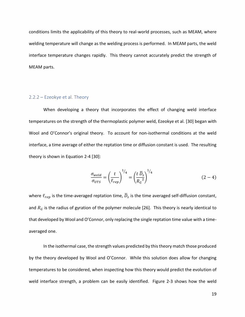
2.2.2 – Ezeokye et al. Theory
When developing a theory that incorporates the effect of changing weld interface
temperatures on the strength of the thermoplastic polymer weld, Ezeokye et al. [30] began with
Wool and O’Connor’s original theory. To account for non-isothermal conditions at the weld
interface, a time average of either the reptation time or diffusion constant is used. The resulting
theory is shown in Equation 2-4 [30]:
𝜎𝑤𝑒𝑙𝑑
𝜎𝑈𝑇𝑆= (
𝑡
𝜏�̅�𝑒𝑝)
14⁄
= (𝑡 �̅�𝑠
𝑅𝐺2)
14⁄
(2 − 4)
where 𝜏�̅�𝑒𝑝 is the time-averaged reptation time, �̅�𝑠 is the time averaged self-diffusion constant,
and 𝑅𝐺 is the radius of gyration of the polymer molecule [26]. This theory is nearly identical to
that developed by Wool and O’Connor, only replacing the single reptation time value with a time-
averaged one.
In the isothermal case, the strength values predicted by this theory match those produced
by the theory developed by Wool and O’Connor. While this solution does allow for changing
temperatures to be considered, when inspecting how this theory would predict the evolution of
weld interface strength, a problem can be easily identified. Figure 2-3 shows how the weld

20
strength predicted by this theory evolves over a single thermal cycle weld process. The weld
interface strength rapidly increases, before decreasing and settling to a single value. This
behavior is due to the use of time-averaged properties in the strength calculations. Specifically,
early in the process, when the weld interface is still hot, the reptation time is short. As the
temperature decreases, the reptation time rapidly increases. However, the short reptation time
at the beginning of the process is causing the time averaged reptation time to report a relatively
low value compared to the process time. As the process progresses the time-averaged reptation
time begins to settle to a near-constant value, resulting in the settling of the predicted weld
strength value.
Figure 2-3: Progression of weld strength ratio over a single cycle weld as predicted by Ezeokye et al.

21
The peak in predicted strength caused by the rapidly changing reptation time is a
troubling result. Strength at the weld interface should monotonically increase over the weld
process. Consider a case where the weld is quenched to a temperature below which molecular
movement would stop, ending weld strength development while the process is at the peak of
the strength over time curve for this theory in the single cycle case demonstrated in Figure 2-3.
The strength reported at this time would be relatively high. If more time is allowed to pass before
the weld is quenched, then the reported strength would actually be lower than the strength in
the previous case. As the weld process progresses, additional polymer molecules diffuse across
the weld interface. Due to the random movement of the reptation driven diffusion, it is possible
that some interface-spanning molecules may move in such a way that they no longer contribute
to strengthening the weld interface, but the overall strength should not decrease at the rate and
magnitude seen in this non-isothermal example.
It is possible that Ezeokye et al. did not see this possible outcome in their experiments.
This theory was developed for use in welding of thermoplastic polymer pipes. A thermal history
where interface temperature increased over the course of the experiment was used [30]. It is
possible that the goal was to accurately determine the amount of time needed to create a fully-
healed weld interface. When applied to a thermal history where temperature history decreases,
as would be seen in the first thermal cycle of an MEAM process, the weld strength evolves as
shown in Figure 2-3. This result shows that this method of weld strength calculation is not
appropriate for determining the strength of MEAM parts.

22
2.2.3 – Bastien and Gillespie Theory
Bastien and Gillespie also use the work of Wool and O’Connor as a basis for their theory
for non-isothermal polymer weld interface strength calculation. To account for changes in the
rate of strength development due to changes in process temperature, the weld process is broken
down into a series of steps. Strength of the weld interface is calculated by summing the strength
development occurring within each individual time step. Each timestep is treated as an
isothermal weld process. The equation used by Bastien and Gillespie to calculate weld interface
strength is shown as Equation 2-5 [31]:
𝜎𝑤𝑒𝑙𝑑
𝜎𝑈𝑇𝑆= ∑
𝑡𝑡+11
4⁄ − 𝑡𝑡1
4⁄
𝜏�̅�𝑒𝑝𝑡
14⁄
𝑡𝑝 Δ𝑡⁄
𝑡=0
(2 − 5)
where tp is the total process time, Δ𝑡 is the size of the time steps used in the strength calculation,
tt is the time when the current time step begins, tt+1 is the time when the next time step begins,
and 𝜏�̅�𝑒𝑝𝑡 is the time averaged reptation time over the current timestep. As with Wool and
O’Connor’s theory, the rate of strength development is controlled by both the diffusion rate
defining reptation time and a ¼ power term. Interestingly, Bastien and Gillespie developed this
theory to simulate weld processes where thermal history began at ambient temperature, mold
compression and friction welding are cited as processes for which this theory was intended to be
used [31].
Figure 2-4 shows how Bastien and Gillespie’s theory predicts weld strength when given a
single cycle thermal history. While strength does increase monotonically, it does so incredibly
quickly. Strength is also allowed to increase to values above the strength of the bulk polymer.

23
While all values above this strength limit could be assumed to simply be equal to the bulk material
strength, the overshoot of the maximum possible strength indicates that this theory may not be
accurately modeling the process of strength development.
Figure 2-4: Progression of weld strength ratio over a single cycle weld as predicted by Bastien and Gillespie.
2.2.4 – Yang and Pitchumani Theory
Yang and Pitchumani take a slightly different approach to determining weld interface
strength. They claim that strength development is modeled too slowly by other theories. Yang
and Pitchumani’s work is based on the idea that diffusion of minor chains, smaller segments of
the entire polymer chain molecule that escape the initial reptation confinement tube first, is
responsible for strength development at the weld interface [27]. As discussed in Section 2.1.1,

24
the ends of the polymer molecule are more likely to escape the confinement tube first. If these
sections are responsible for strength development, then the time necessary for the entire chain
to escape the confinement tube would be irrelevant. So instead of using the reptation time to
determine the rate of diffusion contributing to weld strength development, Yang and Pitchumani
use a “welding time” term, tw. Their equation for weld interface strength is given by Equation 2-
6 [27].
𝜎𝑤𝑒𝑙𝑑
𝜎𝑈𝑇𝑆= [∫
1
𝑡𝑤(𝑇)
𝑡
0
𝑑𝑡]
12⁄
(2 − 6)
The welding time, tw is the experimentally determined time necessary for the weld interface to
become fully healed as a function of tempreature. To account for changes in temperature, the
equation is integrated over the process time, with the welding time changing as a function of
weld interface temperature.
There are issues with the application of Yang and Pitchumani’s theory. First, using an
experimentally determined welding time to drive the rate of strength development requires a
large amount of experimental work to be performed before use of this theory to make any
strength predictions. The reptation time used in all other discussed theories can be obtained in
a single experiment. The second issue with this theory is that it was developed modeling strength
of welded Polyetheretherkeytone (PEEK) matrix composite material. PEEK is a crystalline
thermoplastic polymer. Yang and Pitchumani do not discuss the possible effects of crystal
nucleation or growth on molecular movement at the weld interface. The effects of crystallization
on weld strength development is a research question that is yet to be fully explored.

25
2.3 – Chapter Summary
Each of the discussed polymer weld theories has a flaw that prevents accurate prediction
of MEAM part strength. Wool and O’Connor’s theory is only valid for isothermal welds. In MEAM
parts, the weld interface is not only not isothermal, but it sees several thermal cycles. Weld
interface thermal histories shown in Chapters 5 and 6 show the non-isothermal nature of MEAM
part production.
Ezeokye’s theory attempts to use time averaged material properties to calculate strength
of non-isothermal polymer welds. This property averaging leads to large changes in strength
predictions depending on when the weld process is assumed to be complete. While this method
has been used to make somewhat accurate weld strength predictions [17], the up-and-down
nature of the strength predictions when this theory is applied to a thermal history where
temperature is decreasing is unacceptable.
By splitting the weld process into a series of consecutive time steps, Bastien and Gillespie
have a much better strategy for calculating weld strength for non-isothermal processing
conditions. However, this theory does not include any mechanism to limit weld strength to the
bulk strength of the polymer. Weld strength predictions that overshoot the fully healed condition
call all the strength predictions made by this theory into question.
Yang and Pitchumani take a slightly different approach. They based their strength theory
on experimentally determined amounts of time it takes an isothermal weld to fully heal at various
temperatures. They then use these welding times instead of the reptation time of the polymer
to model the rate of weld strength development. Yang and Pitchumani use the idea that minor

26
chain movement drives weld strength development and suggest that other theories are modeling
weld strength with rates of strength developments that are too low. As with the other presented
theories, Yang and Pitchumani also do not include a mechanism to limit weld strength to the fully
healed value.
Chapter 3 describes work done in weld strength prediction specifically for MEAM parts.
Unlike the work described in Section 1.3, the studies reviewed in Chapter 3 correctly identify the
mechanism by which strength is developed in MEAM parts. Two different models for estimating
MEAM part strength are explored in Chapter 3. This work represents the current state-of-the-
art in MEAM part strength prediction.

27
3 – Contemporary work in MEAM part strength calculation
As the work described in Section 1.3 has shown, consideration must be given to the
mechanism by which strength is developed within MEAM parts to accurately predict part
strength. Contemporary work in this field has concentrated on the weld interface between
adjacent extrudate roads and layers. It is now well understood that the mechanism by which
MEAM parts develop strength is a polymer welding process, in which polymer molecules diffuse
across the interface and become entangled with polymer molecules on both sides of the
interface. While the work described here has made significant strides towards understanding
the mechanical response of MEAM parts, part strength has not been directly calculated.
Work identifying the role of the weld interface in MEAM part strength is summarized in
Section 3.1. The thermal history of the weld interface is a focus point in this work. Thermal
measurements are taken, and the amount of time that molecular diffusion is allowed to occur is
correlated with part strength. Sections 3.2 and 3.3 outline two theories for calculating MEAM
part strength. Coogan and Kazmer’s theory based on the work of Wool and O’Connor is
summarized in Section 3.2. This work is ultimately flawed, due primarily to the inability of Wool
and O’Connor’s theory to calculate the strength of non-isothermal polymer welds. A weld
strength theory specifically for MEAM by McIlroy and Olmsted is discussed in Section 3.3. This
theory aims to calculate the number of entanglements at the weld interface. While this theory
does show promise, it does not directly calculate part strength, only weld-interface-spanning
entanglements. While mechanical properties are directly related to entanglements, this would
be an obstacle for widespread use of this theory. The ideas presented by McIlroy and Olmstead
do provide a good starting point for a more easily applicable theory.
28
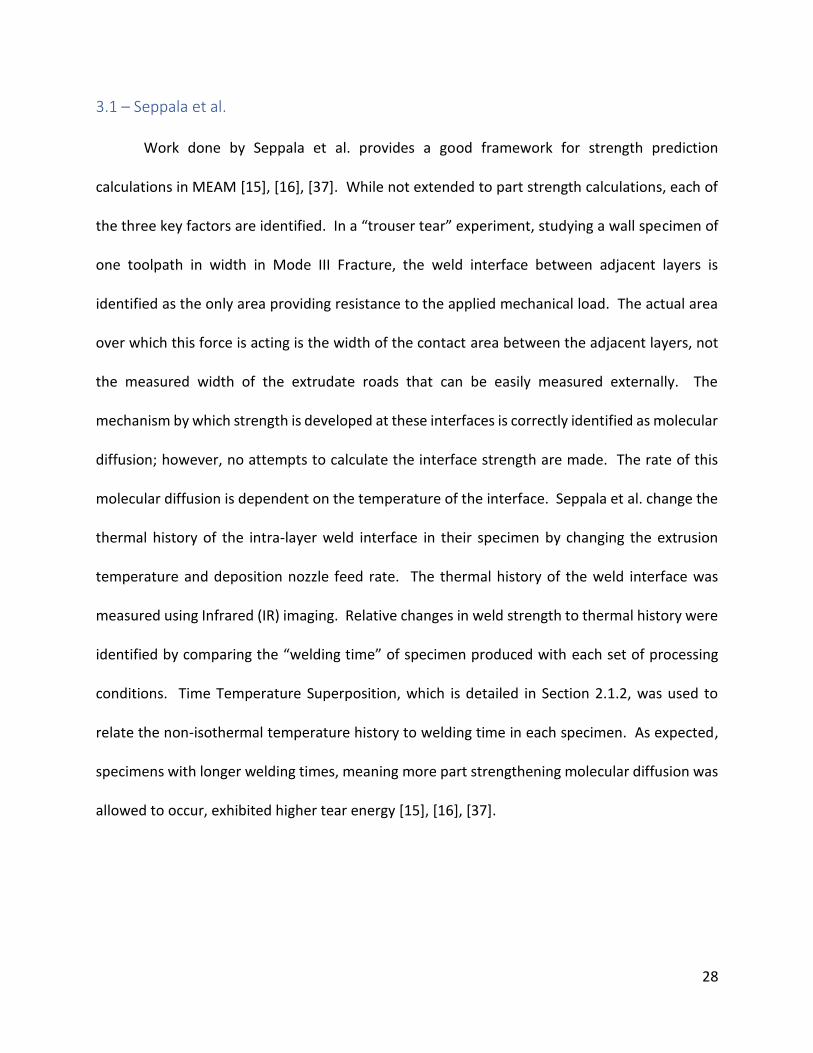
3.1 – Seppala et al.
Work done by Seppala et al. provides a good framework for strength prediction
calculations in MEAM [15], [16], [37]. While not extended to part strength calculations, each of
the three key factors are identified. In a “trouser tear” experiment, studying a wall specimen of
one toolpath in width in Mode III Fracture, the weld interface between adjacent layers is
identified as the only area providing resistance to the applied mechanical load. The actual area
over which this force is acting is the width of the contact area between the adjacent layers, not
the measured width of the extrudate roads that can be easily measured externally. The
mechanism by which strength is developed at these interfaces is correctly identified as molecular
diffusion; however, no attempts to calculate the interface strength are made. The rate of this
molecular diffusion is dependent on the temperature of the interface. Seppala et al. change the
thermal history of the intra-layer weld interface in their specimen by changing the extrusion
temperature and deposition nozzle feed rate. The thermal history of the weld interface was
measured using Infrared (IR) imaging. Relative changes in weld strength to thermal history were
identified by comparing the “welding time” of specimen produced with each set of processing
conditions. Time Temperature Superposition, which is detailed in Section 2.1.2, was used to
relate the non-isothermal temperature history to welding time in each specimen. As expected,
specimens with longer welding times, meaning more part strengthening molecular diffusion was
allowed to occur, exhibited higher tear energy [15], [16], [37].
29
3.2 – Coogan and Kazmer Theory
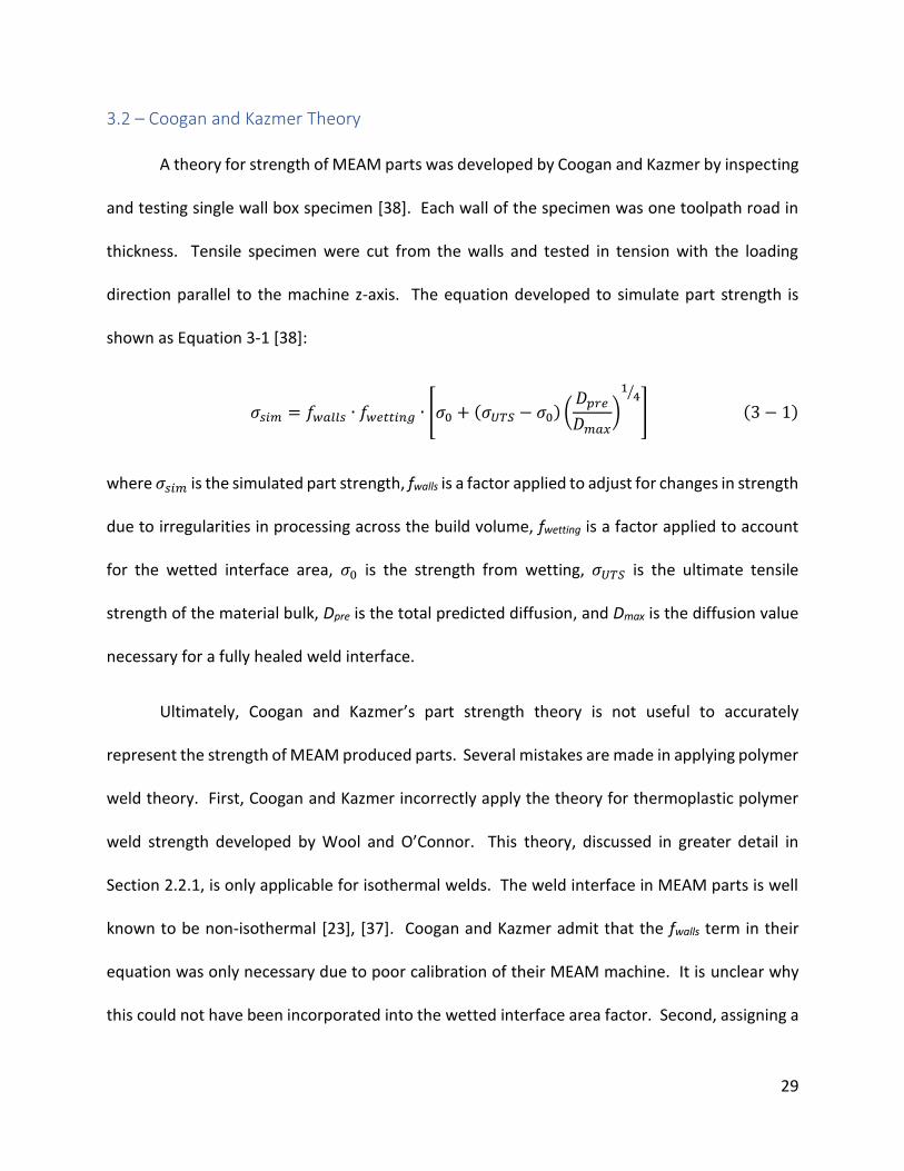
A theory for strength of MEAM parts was developed by Coogan and Kazmer by inspecting
and testing single wall box specimen [38]. Each wall of the specimen was one toolpath road in
thickness. Tensile specimen were cut from the walls and tested in tension with the loading
direction parallel to the machine z-axis. The equation developed to simulate part strength is
shown as Equation 3-1 [38]:
𝜎𝑠𝑖𝑚 = 𝑓𝑤𝑎𝑙𝑙𝑠 ∙ 𝑓𝑤𝑒𝑡𝑡𝑖𝑛𝑔 ∙ [𝜎0 + (𝜎𝑈𝑇𝑆 − 𝜎0) (𝐷𝑝𝑟𝑒
𝐷𝑚𝑎𝑥)
14⁄
] (3 − 1)
where 𝜎𝑠𝑖𝑚 is the simulated part strength, fwalls is a factor applied to adjust for changes in strength
due to irregularities in processing across the build volume, fwetting is a factor applied to account
for the wetted interface area, 𝜎0 is the strength from wetting, 𝜎𝑈𝑇𝑆 is the ultimate tensile
strength of the material bulk, Dpre is the total predicted diffusion, and Dmax is the diffusion value
necessary for a fully healed weld interface.
Ultimately, Coogan and Kazmer’s part strength theory is not useful to accurately
represent the strength of MEAM produced parts. Several mistakes are made in applying polymer
weld theory. First, Coogan and Kazmer incorrectly apply the theory for thermoplastic polymer
weld strength developed by Wool and O’Connor. This theory, discussed in greater detail in
Section 2.2.1, is only applicable for isothermal welds. The weld interface in MEAM parts is well
known to be non-isothermal [23], [37]. Coogan and Kazmer admit that the fwalls term in their
equation was only necessary due to poor calibration of their MEAM machine. It is unclear why
this could not have been incorporated into the wetted interface area factor. Second, assigning a

30
portion of the overall strength of the weld interface to adhesion due to wetting is inconsistent
with the known diffusion mechanism for strength development. In the case where there is no
diffusion occurring between the two weld components, such as if the materials of the two
component pieces were immiscible, there could be some friction force between the two
component parts. If there is any interface-spanning diffusion, this friction force would be
negligible.
Coogan and Kazmer determine the weld strength by calculating the amount of diffusion
that would have occurred during the weld process and comparing that value to the diffusion
value that would represent a fully healed weld. The predicted diffusion value is calculated using
temperature and temperature dependent viscosity values found experimentally using parallel
plate rheometry. The diffusion value where the weld interface would be fully healed was found
by determining the intersection of the UTS of the polymer and diffusion predictions. Coogan and
Kazmer do report a good fit between their model and experimental data, however because the
𝜎0 and Dmax values are found by curve-fitting, this data the validity of this model requires further
testing.
3.3 – McIlroy and Olmsted Theory
McIlroy and Olmsted approach MEAM part strength from a theoretical polymer science
prospective, with a goal of calculating the entanglement density at the weld interface of MEAM
parts [14]. When this entanglement density reaches that of the polymer bulk, the weld will be
fully healed. Even though their simulations indicate that the diffusion distance of an individual
polymer molecule is greater than the reptation tube diameter, McIlroy and Olmsted use both the

31
Rouse model [32] and reptation model [33] to describe the molecular movement that drives
diffusion at the weld interface. This choice is made because their simulations indicate that the
entire polymer molecule does not become fully relaxed. They do conclude that weld penetration
depth does not have an effect on the strength of welds in MEAM parts. The equations they use
to determine weld interface strength in MEAM parts are shown as Equations 3-2 and 3-3 [14].
Equation 3-2 defines the rate of entanglement development at the weld interface:
𝑑𝜐
𝑑𝑡=
1 − 𝜐
𝜏𝑑𝑒𝑞(𝑇(𝑡))
(3 − 2)
where 𝜐 is the relative entanglement number and 𝜏𝑑𝑒𝑞 is the equilibrium reptation time of the
polymer, defined as a function of temperature which changes as the weld process progresses.
Equation 3-3 shows the entanglement at the end of the welding process:
𝜐𝑊 = 1 − (1 − 𝜐𝑑𝑒𝑝(𝑍𝑒𝑞)) 𝑒𝑥𝑝 (− ∫𝑡
𝜏𝑑𝑒𝑞
(𝑇(𝑡))
𝑡𝑔𝑊
𝑡𝑤 𝑑𝑡) (3 − 3)
where 𝜐𝑊 is the final weld entanglement, 𝜐𝑑𝑒𝑝 is the entanglement at deposition, and Zeq is the
equivalent entanglement number of the polymer, which is a function of molecular weight.
McIlroy and Olmsted’s study was purely analytical, and the simulated weld strengths were
not compared to experimental data. The concept explored is a novel one with respect to polymer
weld theories, calculating the local number of entanglements instead of the mechanical property
values. Aside from the fact that this theory has yet to be experimentally verified, there are
several points that would make implementation of this theory a challenge. First, it may not be
clear to the average engineer how to relate weld entanglement to mechanical properties. The

32
𝜐𝑊 value should represent the degree of healing of the weld interface, and therefore the ratio of
the weld strength to bulk material strength, but this is not specifically identified in McIlroy and
Olmsted’s work. Second, the information needed to calculate many of the parameters used in
Equations 3-2 and 3-3 is not always readily available. While reptation time can be determined
experimentally, the molecular weight and radius of gyration are more difficult to determine.
Molecule specific information, such as molecular weight is often considered confidential by the
material manufacturer, and it is not often supplied in material data sheets. McIlroy and Olmsted
also only consider the case where the weld interface is only subjected to one thermal cycle. Weld
interfaces in MEAM parts are often subjected to multiple thermal cycles. However, it appears
that this theory would be flexible enough to handle thermal histories typically measured in
MEAM build processes.

33
4 - Proposed New Weld Strength Theory
For the resulting theory to be widely useful in MEAM part strength predictions, it must
meet the following criteria:
First, the theory must be material agnostic. If the strength theory is constrained to only
one material, then potential use of the theory would be incredibly limited. Validity for only one
use case would also suggest that the theory does not accurately represent the phenomena
responsible for weld strength development.
Second, the theory must be thermal history agnostic. The reptation driven molecular
diffusion that gives polymer welds their strength happens at a rate that is defined by the
temperature of the polymer. At high temperatures, reptation happens relatively quickly. At low
temperatures, reptation happens slowly. The thermal history at a weld interface in a MEAM-
produced part will change from part to part, and it will even vary between different locations
within the same part. The effects of differing thermal histories on part strength is discussed in
detail in Chapter 6.
Third, the theory must use only readily available or easily attainable information. Ideally,
this theory should enable an engineer to make design decisions. Most likely, build simulation
software will be needed to fully assess the impacts of design decisions on part strength; however,
the information needed to perform strength calculations must be readily available. If part
strength calculations require information that is not readily available or difficult to obtain, then
the strength theory is useless to the engineer who should be using it.

34
Fourth, the theory must properly represent the limits of the weld strength. At a fully
healed interface, the strength of the weld is equal to the strength of the bulk material. There
should be no possible set of inputs conditions that results in a weld strength prediction greater
than the strength of the bulk material. The weld theory must accurately represent weld strength
at all stages of the weld process. Including possible predictions over the bulk material strength
or overshooting the end-of-process value before settling would be unacceptable.
4.1 – Derivation
4.1.1 – The Rate of Weld Strength Development
The first step in defining an equation to determine the strength of a thermoplastic
polymer weld is to define the rate at which strength is developed at the weld interface. Rate of
weld strength development is determined using Equation 4-1:
𝑑 (𝜎𝑤𝑒𝑙𝑑
𝜎𝑈𝑇𝑆)
𝑑𝑡= (1 − (
𝜎𝑤
𝜎𝑈𝑇𝑆)) (
1
𝜏𝑟𝑒𝑝) (4 − 1)
where 𝜎𝑤 is the weld strength, 𝜎𝑈𝑇𝑆 is the ultimate tensile strength of the polymer, t is time, and
𝜏𝑟𝑒𝑝 is the reptation time of the polymer.
The rate of strength development is dependent on two factors. The first factor is the rate
of molecular diffusion. As it is assumed that the diffusion distance necessary is larger than the
diameter of the reptation confinement tube, only reptation motion is relevant at this length
scale. With reptation motion alone defining the motion of the polymer molecules, the reptation
time will define the rate of diffusion. The (1
𝜏𝑟𝑒𝑝) term in the rate of strength development

35
accounts for movement of polymer molecules across the weld interface. As with each of the
other weld theories discussed in Chapter 2, the reptation time is the primary driver for the rate
of strength development.
Because the reptation movement of polymer molecules is stochastic, the location where
and time during the weld process when individual molecules cross the weld interface is random.
There are a finite number of locations at the weld interface where a polymer molecule can cross
the weld interface and form interface-spanning entanglements. As the weld process progresses,
the number of available entanglement locations at the weld interface decreases. With a smaller
number of possible entanglement sites available, the probability that a polymer molecule finds
one of these locations is reduced. This is accounted for by including a term that reduces the rate
of weld strength development as weld strength increases.
Picture the weld interface as a hook-and-loop connection with six hoops and six loops,
each numbered 1 through 6. When all six connections are made, the hook-and-loop connection
will be at full strength. Beginning with no connections made, randomly choose one of the hook
and loop pairs to become connected using a six-sided die. If a 1 is rolled, make a connection
between hook #1 and loop #1. Repeat this process until each of the six connections are made,
doing nothing if the random number matches a hook and loop pair that have already been
connected. As more connections are made, the chance that a new connection is made during
each cycle is decreased. The locations where polymer molecules can become entangled on both
sides of the weld interface behaves in the same way. As interface-spanning entanglements are
formed, there are fewer available locations for new connections to be made between the two
component parts to be welded together.

36
The (1 − (𝜎𝑤𝑒𝑙𝑑
𝜎𝑈𝑇𝑆)) term ensures that as weld strength increases, and there are fewer
available locations for interface-spanning entanglements to form, the rate of weld strength
development decreases. This term replaces the ¼ power term introduced by Wool and O’Connor
[25] and used by each of the other weld theory equations. This term in the new weld theory
equation has the same effect as the ¼ power term; i.e., it slows the rate of strength development
as the weld progresses. However, unlike the ¼ power term, this term will limit the predicted
weld strength to that of the fully healed strength value.
This recursive term, relating the rate of weld strength development on the current weld
strength, increases weld strength more slowly than the ¼ power term in the previous theories.
This slower rate of strength development is particularly appropriate for MEAM parts. Much of
the experimental validation work on the weld theories discussed in Chapter 2 was performed
using cut or fractured specimens [25], [30], [31]. By cutting or fracturing the specimens before
welding, the chain end density of the weld interface was increased. When the solid specimen is
cut, polymer molecules are broken. The resulting as-cut surface has many more polymer chain
ends and a locally lower molecular weight than the bulk structure. As discussed in Section 2.1.1,
the end of the polymer chain is most likely to escape the reptation tube first. Increasing the chain
end density increases the rate of diffusion across the weld interface [39], [40].
The weld interfaces in MEAM parts are formed at the interfaces of adjacent roads of as-
extruded material. The surface of the extrudate, and therefore the weld interface, is assumed to
have the same chain end density as the bulk polymer. Molecular diffusion in these areas will
then behave identically to the polymer bulk, where the diffusion distances and timescales are

37
defined by reptation motion [26]. The resulting rate of strength development at any point during
the weld process will then be determined by only by the diffusion rate, (1
𝜏𝑟𝑒𝑝), and the availability
of locations for interface-spanning entanglements, (1 − (𝜎𝑤𝑒𝑙𝑑
𝜎𝑈𝑇𝑆)).
4.1.2 – Strength of an Isothermal Weld
To form an equation for weld strength, the weld strength development rate equation
needs to be integrated. This is done using the separation of variables technique and shown as
Equations 4-2a through 4-2b. First the variables must be moved to opposite sides of the
equations. This is shown as Equation 4-2a:
𝑑 (𝜎𝑤𝑒𝑙𝑑
𝜎𝑈𝑇𝑆)
1 − (𝜎𝑤
𝜎𝑈𝑇𝑆)
=𝑑𝑡
𝜏𝑟𝑒𝑝 (4 − 2𝑎)
This is then integrated with respect to the weld strength ratio and time:
∫𝑑 (
𝜎𝑤𝑒𝑙𝑑
𝜎𝑈𝑇𝑆)
1 − (𝜎𝑤
𝜎𝑈𝑇𝑆)
= ∫𝑑𝑡
𝜏𝑟𝑒𝑝 (4 − 2𝑏)
and evaluating the integrals gives:
−ln (1 − (𝜎𝑤𝑒𝑙𝑑
𝜎𝑈𝑇𝑆)) =
𝑡
𝜏𝑟𝑒𝑝+ 𝐶 (4 − 2𝑐)
where C is the constant of integration. Next each side is multiplied by -1, and an exponential is
applied to both sides.

38
exp (ln (1 − (𝜎𝑤𝑒𝑙𝑑
𝜎𝑈𝑇𝑆))) = exp (
−𝑡
𝜏𝑟𝑒𝑝+ 𝐶) (4 − 2𝑑)
1 − (𝜎𝑤𝑒𝑙𝑑
𝜎𝑈𝑇𝑆) = exp (
−𝑡
𝜏𝑟𝑒𝑝+ 𝐶) (4 − 2𝑒)
The equation can now be solved to give the weld strength ratio.
(𝜎𝑤𝑒𝑙𝑑
𝜎𝑈𝑇𝑆) = 1 − exp (
−𝑡
𝜏𝑟𝑒𝑝+ 𝐶) (4 − 2𝑓)
Initially, the weld will have zero strength. This information can be used to solve for the constant
of integration. Doing so yields an integration constant equal to zero. The resulting equation for
the weld strength ratio is shown as Equation 4-3a. Equation 4-3b shows the equation solved for
the weld strength.
(𝜎𝑤𝑒𝑙𝑑
𝜎𝑈𝑇𝑆) = 1 − exp (
−𝑡
𝜏𝑟𝑒𝑝) (4 − 3𝑎)
𝜎𝑤𝑒𝑙𝑑 = 𝜎𝑈𝑇𝑆 (1 − exp (−𝑡
𝜏𝑟𝑒𝑝) ) (4 − 3𝑏)
While this derivation does provide a concise form of the weld strength equation, it is only
useful for isothermal polymer welds. Equations 4-3a and 4-3b do not allow for a changing
reptation time, which is necessary for non-isothermal conditions. This violates one of the four
requirements described at the beginning of Section 4.1, which requires the weld theory to be
agnostic to thermal history. As any industrial welding process would be non-isothermal, this
equation would not be applicable to any real-world processing scenario, including MEAM. By

39
altering the derivation of the weld strength equation so that a finite integration process is used,
an equation that is capable of calculating weld strength for non-isothermal processing conditions.
4.1.3 – Strength of a Non-Isothermal Weld
The isothermal weld strength theory derived in Section 4.1.2 can be transformed into a
non-isothermal weld strength theory by splitting the non-isothermal weld process into a series
of consecutive isothermal welds. This strategy was also implemented by Bastien and Gillespie
[31]. This is accomplished by integrating the equation defining the rate of strength development
over finite bounds. The bounds of integration are set to the initial and final process states for a
single time step. Equation 4-2b is re-written for finite integration, shown as Equation 4-4a:
∫𝑑 (
𝜎𝑤𝑒𝑙𝑑
𝜎𝑈𝑇𝑆)
1 − (𝜎𝑤𝑒𝑙𝑑
𝜎𝑈𝑇𝑆)
(𝜎𝑤𝑒𝑙𝑑𝜎𝑈𝑇𝑆
)𝑓
(𝜎𝑤𝑒𝑙𝑑𝜎𝑈𝑇𝑆
)𝑖
= ∫𝑑𝑡
𝜏�̅�𝑒𝑝
𝑡𝑓
𝑡𝑖
(4 − 4𝑎)
where (𝜎𝑤𝑒𝑙𝑑
𝜎𝑈𝑇𝑆)
𝑖 is the initial weld strength ratio, (
𝜎𝑤𝑒𝑙𝑑
𝜎𝑈𝑇𝑆)
𝑓 is the final weld strength ratio at the
end of the calculation timestep, ti is the time at the beginning of the calculation, tf is the time at
the end of the calculation timestep, and 𝜏�̅�𝑒𝑝 is the average reptation time over the evaluated
timestep. Evaluating the integral gives:
− [ln (1 − (𝜎𝑤𝑒𝑙𝑑
𝜎𝑈𝑇𝑆)
𝑓
) − ln (1 − (𝜎𝑤𝑒𝑙𝑑
𝜎𝑈𝑇𝑆)
𝑖
)] =𝑡𝑓 − 𝑡𝑖
𝜏�̅�𝑒𝑝 (4 − 4𝑏)
Multiplying by -1 and re-arranging using the properties of the natural algorithm gives:
ln (
1 − (𝜎𝑤𝑒𝑙𝑑
𝜎𝑈𝑇𝑆)
𝑓
1 − (𝜎𝑤𝑒𝑙𝑑
𝜎𝑈𝑇𝑆)
𝑖
) = − (𝑡𝑓 − 𝑡𝑖
𝜏�̅�𝑒𝑝) (4 − 4𝑐)

40
Both sides of the equation are then evaluated as an exponential.
exp [ln (
1 − (𝜎𝑤𝑒𝑙𝑑
𝜎𝑈𝑇𝑆)
𝑓
1 − (𝜎𝑤𝑒𝑙𝑑
𝜎𝑈𝑇𝑆)
𝑖
)] = exp [− (𝑡𝑓 − 𝑡𝑖
𝜏�̅�𝑒𝑝)] (4 − 4𝑑)
1 − (𝜎𝑤𝑒𝑙𝑑
𝜎𝑈𝑇𝑆)
𝑓
1 − (𝜎𝑤𝑒𝑙𝑑
𝜎𝑈𝑇𝑆)
𝑖
= exp [− (𝑡𝑓 − 𝑡𝑖
𝜏�̅�𝑒𝑝)] (4 − 4𝑒)
Performing further algebra:
1 − (𝜎𝑤𝑒𝑙𝑑
𝜎𝑈𝑇𝑆)
𝑓
= (1 − (𝜎𝑤𝑒𝑙𝑑
𝜎𝑈𝑇𝑆)
𝑖
) exp [− (𝑡𝑓 − 𝑡𝑖
𝜏�̅�𝑒𝑝)] (4 − 4𝑓)
The weld strength ratio and the end of the time step can now be solved for directly, as shown in
Equation 4-5a. Equation 4-5b shows an alternate form of the equation where weld strength at
the end of the time step is calculated directly.
(𝜎𝑤𝑒𝑙𝑑
𝜎𝑈𝑇𝑆)
𝑓
= 1 − (1 − (𝜎𝑤𝑒𝑙𝑑
𝜎𝑈𝑇𝑆)
𝑖
) exp [− (𝑡𝑓 − 𝑡𝑖
𝜏�̅�𝑒𝑝)] (4 − 5𝑎)
𝜎𝑤𝑒𝑙𝑑𝑓= 𝜎𝑈𝑇𝑆 − (𝜎𝑈𝑇𝑆 − 𝜎𝑤𝑒𝑙𝑑𝑖
)exp [− (𝑡𝑓 − 𝑡𝑖
𝜏�̅�𝑒𝑝)] (4 − 5𝑏)
Here 𝜎𝑤𝑖 is the initial weld strength, and 𝜎𝑤𝑓
is the final weld strength during this calculation
step. Subsequent calculation steps will use this 𝜎𝑤𝑓 as the initial weld strength and provide a
new weld strength output. This process will be repeated for the entire weld process. The final
weld strength in the last calculation step is the value that is taken as the strength of the weld
interface.

41
Now that a method for calculating the strength of the weld interface has been
established, it needs to be checked against the four requirements defined at the beginning of this
chapter. The first requirement is met, as the reptation time is the only piece of material-specific
information required to determine weld strength using this theory. The reptation time is
different for each thermoplastic polymer; however, this is a measurable quality of all
thermoplastics.
The second requirement is that the theory must be agnostic to thermal history. By
splitting the weld process into steps that are calculated independently, this theory can be used
to calculate the strength of a weld interface with any thermal history. Changes in temperature
are accounted for by changes in the reptation time of the polymer. For each calculation step, the
reptation time used is the average reptation time over the calculation time. One requirement
for accurate strength calculations is that the time steps be evaluated in the correct order, as each
weld strength calculation requires the state of weld strength at the beginning of the time step.
The third requirement is for each of the weld strength calculation inputs to be easily
obtainable information. The inputs to this weld strength equation are the reptation time of the
polymer as a function of temperature, the temperature history of the weld interface, the UTS of
the polymer, and the weld strength at the beginning of the calculation time step. The reptation
time as a function of temperature can be found using a parallel plate rheometry experiment, as
described in Section 5.1. The thermal history of the weld interface can either be measured
directly, as described in Section 5.3, or simulated, as discussed in Section 5.4. The UTS of the
polymer is commonly supplied by the material supplier. The weld strength output from the

42
previous step of weld strength calculation is used as the initial weld strength in the current
calculation step.
The fourth requirement is that the weld strength must be accurately represented
throughout the weld process. While this will ultimately need to be experimentally determined,
as shown in Sections 4.3 and 5.3, this theory does offer advantages over other theories. The
(1 − (𝜎𝑤𝑒𝑙𝑑
𝜎𝑈𝑇𝑆)) term in the equation, or the rate of weld strength development, ensures that the
fully healed condition is the maximum strength that can be predicted by this theory. These weld
strength equations also ensure that the predicted weld strength will not decrease under certain
conditions as the weld process progresses.
4.2 – Loading Direction Independence of Polymer Welds
While not explicitly stated within any of the cited polymer weld strength work, the
independence of weld strength to loading direction is implied. Work done by Wool and O’Connor
examined polymer weld interfaces under both tensile [25], [29] and shear [35] loading conditions.
Experiments testing both loading conditions, tensile and shear, led to the same weld strength
equations. The other theories examined in Chapter 3 were also tested using a mix of both tensile,
Exeokye et al. [30], and shear, Yang and Pitchumani [27], loading conditions. In each of these
papers, the loading direction of the weld interface is not even discussed. Because amorphous
thermoplastic polymers do not have an organized internal structure, there is no difference
between tensile and shear loading on the entanglements that provide strength to the material

43
bulk. The randomly oriented molecules and entanglements will respond to a mechanical stimulus
in the same manner regardless of the direction that the stimulus is applied.
The weld interface introduces an orientation specific feature to the thermoplastic
polymer structure. However, the only difference between this interface and the amorphous
polymer bulk is the entanglement density. Therefore, as implied by prior work in this area, the
strength of the weld will not be affected by the direction of the applied load. The weld interface
will hold the same load before failing regardless of the loading direction. This property of
polymer weld interfaces will be investigated with the tensile experiments on MEAM parts with
varying toolpath orientations. The results of these experiments are discussed in Section 5.3.
Now that a theory for weld strength in MEAM parts has been established, it needs to be
tested. Chapter 5 discusses the process used to implement the weld theory into MEAM part
strength calculations, incorporating the structure of the MEAM part into the analysis. These
strength estimations generated using the weld theory are then compared to experimental
results. Close correlation between the calculated and experimental strength values is shown.

44
5 – MEAM part strength predictions
Even with an accurate calculation of the strength of welds between adjacent roads and
layers within a MEAM part, additional information is still needed to determine the strength of
the part as a whole. The strength of the internal welds is a key element to this calculation, but
other factors must be considered. The internal geometry of the part and the orientation of the
layers, and extrudate roads within those layers, relative to the loading direction are two
additional pieces of information necessary to provide accurate part strength predictions. The
internal geometry of the part provides the area within each layer where welding has occurred
between adjacent layers and extrudate roads. Orientation of roads and layers relative to the
applied load is necessary to determine which weld interfaces are stressed during loading.
Theoretical and experimental strength calculations of MEAM parts are carried out for the
uniaxial tension loading condition in this chapter. ASTM D638 is used as the test standard,
defining specimen geometry and experimental procedure. Specifically, ASTM D638 Type I
specimens are used in this experiment. To ensure that this part strength calculation method is
valid across multiple build conditions, multiple toolpath orientations are used. This study only
considers specimen with 100% infill density. Response of MEAM parts with less than 100% infill
density is discussed in Chapter 7.
Changing toolpath orientation not only changes the orientation of the weld interface with
respect to the loading direction, but also the thermal history. When the toolpath orientation
changes relative to the gage region of the tensile specimen, the length of each toolpath changes.
This change in toolpath length has a significant effect on the thermal history of the weld interface.

45
As toolpath length increases, the amount of time between adjacent depositions also increases.
Because it takes the deposition nozzle longer to complete each toolpath, the previously
deposited extrudate has a longer period of time to cool down. The cooler deposited material
reduces the temperature of the interface when the new extrudate is deposited. As discussed in
Section 2.1.1, at cooler temperatures reptation movement of the polymer molecules happens
more slowly, reducing the rate of diffusion across the interface, which results in a weaker weld
interface.
5.1 – Applying the new weld strength theory to MEAM parts
The strength of a MEAM part must be considered as a complete structure, not a single
weld interface. The orientation of toolpaths and weld interfaces relative to the loading direction
must be considered. In the case of the tensile specimen, if any toolpaths or layers are parallel to
the gage region of the tensile specimen, then the weld interface between these extrudate roads
and layers is not loaded. If the extrudate road is not parallel to the loading direction, then the
weld interfaces transfer the mechanical loads between the adjacent roads and layers. Since
these weld interfaces will not be as strong as the bulk material, they will limit and thus define the
strength of the MEAM part. The strength of this weld interface can be calculated using the weld
theory proposed in Chapter 4.
To calculate weld strength using Equation 4-5b, three pieces of information are needed:
(1) the UTS of the polymer, (2) the reptation time of the polymer as a function of temperature,
and (3) the thermal history of the weld interface. UTS values provided by the feedstock material
manufacturer are used in the calculation. Using experimental data and Time-Temperature

46
Superposition, as discussed in Sections 2.1.1 and 2.1.2, the reptation relaxation time can be found
as a function of temperature:
𝜏𝑟𝑒𝑝(𝑇) = 𝜏𝑟𝑒𝑝(𝑇𝑟𝑒𝑓) ⋅ 𝑎𝑇 (5 − 1)
where 𝜏𝑟𝑒𝑝 is the reptation time of the polymer, T is the temperature of interest, Tref is the
reference temperature, and aT is the time shift factor. Incorporating the WLF equation for the
time shift factor from Equation 2-1 gives a closed form equation for reptation time as a function
of temperature shown as Equation 5-2:
𝜏𝑟𝑒𝑝(𝑇) = 𝜏𝑟𝑒𝑝(𝑇𝑟𝑒𝑓) ⋅ exp [−𝐶1(𝑇 − 𝑇𝑟𝑒𝑓)
𝐶2 + (𝑇 − 𝑇𝑟𝑒𝑓)] (5 − 2)
where C1 and C2 are the WLF equation constants. The reptation time at a reference temperature
and WLF equation constants can be found using the same parallel plate rheometry experiment.
As described in Section 2.1.1, the reptation relaxation time of the polymer is equal to the
inverse of the low frequency crossing point of the storage modulus (G’) and loss modulus (G”). A
parallel plate rheology experiment, where a small disc of the material of interest is loaded in
reciprocating shear, can measure G’ and G” across a wide range of deformation frequencies and
temperatures. An isothermal frequency sweep is performed at several different temperatures,
and Time-Temperature Superposition (TTS) is used to combine the data measured at each
temperature into a master curve for G’ and G”. Data should be taken at temperatures ranging
from the maximum extrusion temperature used in the MEAM processing of the polymer to the
polymer’s glass transition temperature (Tg). The shift factors used to form the master curve are
then fit to the WLF equation to find the WLF constants. A temperature at which the low

47
frequency crossing point of G’ and G” lies within the experimental data is chosen to be the
reference temperature. The reptation time at this temperature is then used in Equation 5-2.
With all the necessary information, the reptation time can now be found at any temperature
between the extrusion temperature and Tg of the polymer, the range over which the weld
interface will be developing strength.
The weld interface temperatures in this study were measured experimentally during
MEAM production of representative parts. Thermal history could be found by other means, such
as build simulation [41]. To get a complete and accurate thermal history, the results of two
different temperature measurement experiments were conducted. Temperature data from the
initial deposition of material was obtained using Infrared (IR) imaging. Due to difficulties in
directly measuring the temperature of the weld interface, due to obstructions caused by the
deposition nozzle and the y-axis of the machine moving the area of interest, a representative
experiment was carried out. A wall with the thickness of a single extrudate road was constructed,
similar to the IR temperature measurements by Seppala et al. [37]. However, this wall specimen
was built such that each pass of the nozzle would be identical to the toolpaths used to build the
gage region of the tensile specimen. The thermal history at the interface between layers of this
wall specimen are representative of the thermal history of the interface between adjacent roads
within one layer in the gage region of a tensile specimen. This data was used to determine the
thermal history of the weld interface during the deposition of the new layer.
As the center of the toolpath has the longest amount of time between deposition of the
two extrudate roads that make up the interface, this location cools down most before material
is added. This location will then have the thermal history least conducive to developing weld

48
strength. The entire weld interface is assumed to have the same thermal history as this worst-
case location.
Thermal history data for subsequent layers in the build is found by embedding a type-J
thermocouple within the tensile specimen as it was built. Figure 5-1 shows the thermocouple
embedded in a tensile specimen before additional material was deposited above it. The
temperature data from this thermocouple was used to determine the thermal history of the weld
interface beginning with the layer after the interface of interest was deposited. As with the IR
measurements, the thermocouple measurements are taken at the center of the specimen,
providing the worst-case thermal history. The data from this experiment is taken to be
representative of the thermal history of the as-built tensile specimens. The presence of the
thermocouple, and the pause in the build process necessary to insert it into the part, significantly
weaken the as-built parts [42]. The thermal history from these specimens is used to calculate
strength in the specimens built without the embedded thermocouple.
Figure 5-1: Image of a type J thermocouple placed between the 3rd and 4th layers of a 90° toolpath orientation tensile specimen.
The thermal data from these two temperature measurement experiments was then
combined to provide a thermal history for the entire build. Using Equation 5-2 to determine

49
reptation time at any point in the interface thermal history, Equation 4-5b is used to calculate
the strength of the weld interface between two adjacent extrudate roads in the gage region of
the tensile specimen. Now that the strength of the weld interface has been calculated, the
strength of the entire MEAM part can be determined.
5.2 – Calculating total part strength predictions
In a typical MEAM part, the weld interfaces are responsible for the largest share of the
mechanical strength of the part, but they are not always the sole contributor. Depending on the
loading condition and build strategy used to produce the part, other features will contribute to
part strength. In the case where layer interfaces are loaded, the weld interfaces between the
adjacent layers are the only contributor to part strength. When parts are loaded parallel to the
layer planes, the loading condition becomes a bit more complicated. This is due to the changing
orientation of the extrudate roads, and therefore the weld interfaces, relative to the direction of
applied load. Due to changes in thermal history and possible changes in build strategy, the
strength of each layer of the part must be calculated individually. These layer component
strengths are then combined to determine the total part strength.
In the case of a tensile specimen, there are two possible modes of failure that must be
considered: (1) failure along a weld interface and (2) failure across the minimum cross-sectional
area perpendicular to the applied load. An illustration where these two failure modes occur is
shown in Figure 5-2. Each of the two possible failure modes are considered for each layer. The
failure mode that results in the smaller predicted strength is used in whole part strength
predictions. Figure 5-3 shows an example of each of the two failure modes. A +/- 30° infill

50
toolpath orientation specimen exhibits perpendicular cross-section failure, and a +/- 45° infill
toolpath orientation PC specimen exhibits weld interface failure.
Figure 5-2: An illustration of the two possible fracture surfaces used in MEAM part strength calculation. Weld interface failure will occur along the green line. Minimum cross-section failure will occur along the red line.
Figure 5-3: Fracture surface location of an ABS +/- 30° build orientation specimen, shown above, and a +/- 45° build orientation PC specimen, shown at the bottom of the image. The +/- 30° ABS specimen exhibits perpendicular cross-section failure. The +/- 45° PC specimen exhibits weld interface failure.

51
5.2.1 – Weld interface Failure
The first possible failure mode is weld interface failure, where part failure initiates within
the weld interface. Part strength is calculated along a surface that runs along the weld interface
between two adjacent infill roads and, in the case of a tensile specimen, through the perimeter
roads perpendicular to the loading direction. This fracture surface is shown as a green line in
Figure 5-2. Figure 5-4 shows the cross section of this fracture surface for one layer. Because the
perimeter roads are parallel to the loading direction, they will have a strength equal to the UTS
of the bulk thermoplastic polymer. The perimeter roads are shown in blue in Figure 5-4. Strength
of the weld interface, shown in green in Figure 5-4, is determined using the weld strength theory
presented in Chapter 4.
Figure 5-4: An illustration of the calculation fracture surface for weld interface fracture of a tensile specimen produced with two perimeter roads. The cross section of the perimeter roads are shown in blue and the weld interface is shown in green.
As shown in Figure 5-4, the actual weld interface area is smaller than what would be
expected, as it is smaller than the layer height. This is due to the cross-sectional geometry of the
as-deposited extrudate. Because material is extruded from a round nozzle orifice, it cannot

52
completely fill the rectangular intended voxel. Figure 5-5 illustrates the disparity between the
rectangular voxel and the cross-section of the extrudate intended to fill that voxel. Because the
voxel is not completely filled with material, the weld interface area between two adjacent roads
and layers is also smaller than would be expected for the intended geometry of the part. The
minimum cross-sectional area is also reduced due to this phenomenon.
Figure 5-5: An illustration of the cross-section of deposited extrudate within the voxel it is intended to fill.
The strength of the fracture surface is determined by adding the strength of the perimeter
roads and the weld interface. The maximum force that the layer can withstand is calculated using
Equation 5-3:
𝐹𝑙𝑎𝑦𝑒𝑟,𝑤𝑒𝑙𝑑 = 𝐴𝑤𝑒𝑙𝑑𝜎𝑤𝑒𝑙𝑑 + 𝐴𝑝𝑒𝑟𝜎𝑈𝑇𝑆 (5 − 3)
where Flayer,weld is the maximum force the layer can withstand before failure, Aweld is the weld
interface area, 𝜎𝑤𝑒𝑙𝑑 is the weld strength, Aper is the total cross-sectional area of the perimeter
roads, and 𝜎𝑈𝑇𝑆 is the UTS of the polymer. As the thermal history will be different for each layer,
the weld interface failure mode strength must be calculated for each layer in the part individually.
Because the weld interface area changes with infill direction, there are situations where the
maximum force along the weld interface fracture surface exceeds the force necessary to cause

53
failure in the bulk polymer in the gage region of the tensile bar. In this case, the minimum cross-
section fracture failure force must be considered.
5.2.2 – Perpendicular Cross-Section Failure
The second possibility for fracture in an MEAM part is fracture across the part
perpendicular to the applied load, the minimum cross-sectional area orthogonal to the loading
direction. In this case, the material within the MEAM part behaves as it would in a conventionally
manufactured part. However, the reduced cross-sectional area due to the void space caused by
the extrusion process, as illustrated in Figure 5-5, causes the structure to be less strong than a
part with a completely filled cross-section. Figure 5-6 illustrates this minimum cross-section for
one layer of a tensile specimen produced with two perimeter roads.
Figure 5-6: An illustration of the calculation fracture surface for minimum cross-section fracture of a tensile specimen produced with two perimeter roads. The cross section of the perimeter roads are shown in blue and the cross-section of the infill roads are shown in red.

54
As shown in Figure 5-6, the cross-section of the infill roads relative to the calculation
cross-section may be different than the cross section of the perimeter roads. This is not due to
a change in the width of the deposited extrudate. The area of the intersection of the layer
calculation fracture surface plane, illustrated using a red line in Figure 5-2, with the cross section
of the infill road is larger than the as-extruded cross-section. Because the calculation cross-
section is not always aligned with all of the extrudate roads, the calculation cross-section must
be determined by projecting the extrudate cross-section onto the cross-section perpendicular to
the applied load. In Figure 5-6, the perimeter roads, shown in blue, are perpendicular to the
minimum cross-section. The infill roads, shown in red are not. The total area of material in the
cross-section must be calculated to accurately determine the failure load for this layer.
The weld interface does not impact the strength in this failure mode. Because the weld
depth is so small, no more than twice the diameter of the reptation tube of the polymer molecule
[14], the area of reduced entanglement density in this cross section is negligible. All material is
assumed to have strength equal to the UTS of the polymer. Because the strength of the weld
interface does not effect the strength of this failure mode, this is the maximum possible strength
for this layer. Failure load for the layer in the minimum cross-section is calculated using Equation
5-4:
𝐹𝑙𝑎𝑦𝑒𝑟,𝑚𝑎𝑥 = (𝐴𝑖𝑛𝑓𝑖𝑙𝑙,⊥ + 𝐴𝑝𝑒𝑟) ∙ 𝜎𝑈𝑇𝑆 (5 − 4)
where Flayer,max is the maximum possible layer failure load, as calculated using the minimum cross-
section failure mode, 𝐴𝑖𝑛𝑓𝑖𝑙𝑙,⊥ is the area of the infill perpendicular to the calculation plane, Aper
is the perimeter area, and 𝜎𝑈𝑇𝑆 is the UTS of the polymer.

55
5.2.3 – Determining total part strength
Strength of the entire part is determined by taking the sum of each of the individual layer
failure loads and dividing that by the as-designed cross-sectional area. The strength of each layer
must be determined by comparing the maximum loads for the two possible failure modes. The
smaller maximum load value is taken as the strength of the layer. Equation 5-5 summarizes this
process:
𝐹𝑀𝐸𝐴𝑀 = ∑ 𝐹𝑙𝑎𝑦𝑒𝑟,𝑤𝑒𝑙𝑑 ∧
𝑀
𝑙𝑎𝑦𝑒𝑟=1
𝐹𝑙𝑎𝑦𝑒𝑟,𝑚𝑎𝑥 (5 − 5)
where FMEAM is the force necessary to cause failure in the MEAM part, layer represents the layer
number, and M is the total number of layers.1 Strength of the MEAM part is calculated using
Equation 5-6:
𝜎𝑀𝐸𝐴𝑀 =𝐹𝑀𝐸𝐴𝑀
𝐴𝑑𝑒𝑠𝑖𝑔𝑛
(5 − 6)
where 𝜎𝑀𝐸𝐴𝑀 is the MEAM part strength and Adesign is the as-designed cross-sectional area.
5.3 – Experimental Validation
Mechanical testing was performed to validate the proposed part strength calculation
theory. Five ASTM D638 Type I tensile specimens were produced using varying materials and
material deposition strategies. Commercially available Acrylonitrile Butadiene Styrene (ABS) and
1 The ∧ operator indicates a minimum operation. In this case, the smaller of the two failure force values is to be used in calculation

56
Polycarbonate (PC). Each material was supplied as 2.85mm diameter filament feedstock.
Material properties used in the strength calculations are listed in Table 5-1. Material
manufacturer supplied UTS values were used. Reptation time and WLF equation constants were
determined experimentally using a parallel plate rheometry experiment, Using a Rheometric
Scientific ARES-LS (TA Instruments, New Castle, DE, USA) rheometer. Isothermal frequency
sweeps were performed at 10° C intervals beginning at the maximum MEAM processing
temperature of the polymer and ending just above the Tg of the polymer.
Table 5-1: Material properties used in part strength calculations.
Material UTS Tref τrep (Tref) C1 C2
ABS 43 MPa 175 °C 0.631 sec 6.428 114.9
PC 65.4 MPa 205 °C 0.10 sec 4.017 96.99
Each MEAM test specimen was produced on a Mendel Max 3 (Maker’s Tool Works, OK,
USA) MEAM machine, equipped with a 0.4 mm diameter nozzle. The gcode used to produce the
specimen as generated using a MATLAB script. Processing parameters used for each material are
listed in Table 5-2. As per ASTM D638, a 5 mm/min strain rate was used in tensile experiments.
Table 5-2: Build parameters used to produce tensile specimens.
Build Parameter ABS PC
Nozzle Temp. 230° C 285° C
Build Plate Temp. 115° C 150° C
Nozzle Travel Speed 60 mm/s 60 mm/s
Layer Height 0.2 mm 0.2 mm
Extrudate Width 0.4 mm 0.4 mm
Extrusion Factor [43] 1.02 1.04

57
Strength calculations were performed using the measured and supplied material
information, experimentally measured thermal history, and cross-sectional geometry
information which was measured from fractured specimens. Thermal histories were measured
in two steps. Temperature of the weld interface during the deposition layer was measured using
IR imaging. An Optris PI 400 (OptrisGmbH, Berlin, Germany) IR camera was used to capture the
first layer thermal data at 80 Hz. Thermal history of the wend interface of interest during
deposition of subsequent layers was measured using a type J thermocouple embedded in the
gage region of the tensile specimen. Thermocouple data was captured using a Dataq DI-245
(Dataq Instruments Inc., Akron, OH, USA) at 100 Hz. Thermal history was measured using a
representative sample, as the included thermocouple would cause a stress concentration, and
results would not be representative of a typical MEAM part. Thermal history of an ABS +/- 45°
infill toolpath orientation specimen is shown in Figure 5-7.

58
Figure 5-7: Thermal history of the weld interface at the 4th layer in an ABS +/- 45° infill orientation tensile specimen.
Thermal history measurements from the 4th layer of a tensile specimen were used in
strength calculations. Measurements of thermal histories of subsequent layers showed that the
thermal history was nearly identical above the Tg of the polymer, where weld-strengthening
diffusion can occur, only with fewer thermal cycles. For ease of calculation, measurements from
the 4th layer of a specimen were used to calculate the weld strength in each layer, with the
thermal history truncated to accurately represent each layer. Weld strength progression through
the first 3 layers after extrudate deposition of an ABS +/- 45° infill toolpath orientation specimen
is shown in Figure 5-8.

59
Figure 5-8: Thermal history and weld strength fraction of the first 3 layers after deposition in an ABS +/- 45° toolpath orientation tensile specimen.
As shown in Figure 5-8, the weld interface in the +/- 45° infill toolpath orientation
specimen nears the fully-healed condition after 3 layers of material deposition. To properly test
this weld strength theory, multiple thermal histories are tested. A discontinuous build strategy
was used to alter the thermal history, and the effects of build discontinuities are discussed in
detail in Chapter 6. Thermal history and weld strength progression of the first 3 layers after
deposition in one of these discontinuous specimens is shown in Figure 5-9. As shown, the weld
strength is much lower in this specimen due to the modified thermal history.

60
Figure 5-9: Thermal history and weld strength progression of an ABS tensile specimen with 90° infill toolpath orientation and discontinuous build strategy.
Using the weld strength values for each layer, the total part strength is determined using
the method described in Section 5.2. Using the 90° discontinuous specimen as an example, Table
5-3 lists the area measurements used in the part strength calculations. Table 5-4 lists the
calculated maximum load values for both possible failure modes for each layer.
Table 5-3: Area Measurements used in 90° discontinuous build tensile specimen strength calculations.
Calculation Parameter Value
As-Designed Area - total 41.6 mm2
Layer Weld Area 1.44 mm2
Layer Perimeter Cross-Sectional Area 0.314 mm2
Perpendicular Cross-Sectional Area 2.55 mm2
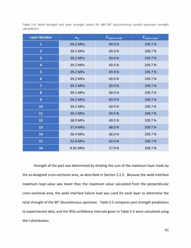
61
Table 5-4: Weld strength and layer strength values for ABS 90° discontinuous tensile specimen strength calculations.
Layer Number 𝝈𝒘 𝑭𝒍𝒂𝒚𝒆𝒓,𝒘𝒆𝒍𝒅 𝑭𝒍𝒂𝒚𝒆𝒓,𝒎𝒂𝒙
1 39.2 MPa 69.9 N 109.7 N
2 39.2 MPa 69.9 N 109.7 N
3 39.2 MPa 69.9 N 109.7 N
4 39.2 MPa 69.9 N 109.7 N
5 39.2 MPa 69.9 N 109.7 N
6 39.2 MPa 69.9 N 109.7 N
7 39.2 MPa 69.9 N 109.7 N
8 39.2 MPa 69.9 N 109.7 N
9 39.2 MPa 69.9 N 109.7 N
10 39.2 MPa 69.9 N 109.7 N
11 39.2 MPa 69.9 N 109.7 N
12 38.9 MPa 69.5 N 109.7 N
13 37.9 MPa 68.0 N 109.7 N
14 36.4 MPa 66.0 N 109.7 N
15 32.6 MPa 60.4 N 109.7 N
16 9.91 MPa 27.9 N 109.7 N
Strength of the part was determined by dividing the sum of the maximum layer loads by
the as-designed cross-sectional area, as described in Section 5.2.3. Because the weld interface
maximum load value was lower than the maximum value calculated from the perpendicular
cross-sectional area, the weld interface failure load was used for each layer to determine the
total strength of the 90° discontinuous specimen. Table 5-5 compares part strength predictions
to experimental data, and the 95% confidence intervals given in Table 5-5 were calculated using
the t-distribution.

62
Table 5-5: Experimental and predicted part strength values for various materials and build strategies.
Build Info Experimental Strength Predicted Strength % Difference
PC - ± 45° Continuous 54.4 ± 4.44 MPa 56.3 MPa 3.37 %
ABS - ± 45° Continuous 38.6 ± 1.35 MPa 38.8 MPa 0.38 %
ABS - 45° Discontinuous
35.6 ± 1.88 MPa 37.1 MPa 4.21%
ABS - 90° Continuous 33.6 ± 0.94 MPa 32.3 MPa 3.80 %
ABS - 90° Discontinuous
25.9 ± 1.80 MPa 25.5 MPa 1.48 %
ABS - 0°/90° Continuous
35.9 ± 1.98 MPa 37.1 MPa 3.23 %
ABS - 0°/90° Discontinuous
36.4 ± 0.94 MPa 35.3 MPa 3.09 %
ABS - ± 30° Continuous 40.6 ± 0.72 MPa 40.2 MPa 1.00 %
ABS - ± 30° Discontinuous
37.9 ± 2.44 MPa 39.8 MPa 4.79 %
As shown in Table 5-5, the part strength predictions were very close to the experimental
part strengths across multiple materials. Each strength prediction was within 5% of the
experimental strength, with the part strength theory predicting part strengths within 1% of the
experimental strength in two different build conditions. Only the strength prediction for the
0°/90° discontinuous specimen fell outside the 95% confidence window for the experimental
results. Accurate estimates of MEAM part strengths signify that this theory can be useful in the
part design process.
5.4 – Future Implementation
While this strength calculation method may seem somewhat tedious when calculating
the strength of parts in the design process, as it necessitates the collection of thermal history

63
data specific to the part, the time-step based approach could be easily implemented into build
simulation software. If thermal history could be modeled using the gcode used to build the part
and polymer specific information was readily available, then accurate predictions of as-built part
strength could be made. For complex geometry parts, varying thermal histories would cause
strength predictions to vary throughout the part. Effects of build strategy and part geometry on
thermal history and part strength are discussed in detail in Chapter 6.
Local strength predictions generated directly from gcode would be a powerful tool for
engineers and designers. Accurate strength predictions would improve confidence in the MEAM
process necessary to be used as an end-use part manufacturing process. The ability to calculate
and visualize how design decisions effect MEAM part strength would facilitate design
optimization, as engineers would have a tool available to visualize how their design and process
parameter decisions affect the mechanical strength of the as-built part. This theory could also
be combined with topology optimization software, where the part geometry, gcode, thermal
history, and resulting part strength would all be estimated during the optimization. The final
design would be optimized for both the use case and the manufacturing process.
Widespread use of this theory would inspire feedstock material suppliers to list the
reference reptation time and WLF constants on their material data sheets. Providing this
information would allow for widespread use of the presented strength calculation method, as it
is currently limited to those who have the equipment necessary to obtain reptation time
experimentally. Providing the design engineer with the information and tools necessary to
generate accurate MEAM part strength predictions would elevate this technology from a
prototyping process to an end-use part manufacturing process.

64
In the next chapter, effects of changing the deposition strategy on the mechanical
properties of MEAM parts is studied. Changing the deposition strategy changes the thermal
history of the part. As discussed in Chapter 5, thermal history is a very important component to
strength of MEAM parts. Comparisons are made between the idealized case typically used for
materials testing and the case of complex geometry parts. Changing the geometry of the part
will change the deposition strategy, which changes the thermal history of the part, which changes
the strength of the part.

65
6 – Toolpath dependence of MEAM part strength
As described in Chapter 5, the three factors that determine the strength of weld interfaces
within MEAM parts: (1) the reptation time of the polymer, (2) the geometry of the weld interface,
and (3) the thermal history of the weld interface. In a typical manufacturing process, when
producing two different parts using the same processing parameters the mechanical properties
of these two parts are expected to be the same. This is not true in MEAM. Holding process
parameters constant only ensures that two of the three factors in weld interface strength remain
the same: (1) the polymer rheology, assuming the same polymer is used, and (2) the geometry
of the weld interface. Two different parts made with the same process parameters will most
likely have different thermal histories. Figure 6-1 shows one layer of two parts with different
geometries. The longer toolpaths in Figure 6-1 (B) will result in a change in thermal history due
to the longer amount of time need to complete each toolpath. This change in thermal history
would be caused by the differences in geometry between the two parts.
Figure 6-1: Toolpath illustrations for two parts with different geometries.

66
Changing toolpath orientation within a part can also change the thermal history. Consider
the sample toolpaths shown for two layers of a simple geometry part shown in Figure 6-2. Even
though the two layers are built using the same polymer, on the same machine, using the same
build parameters, with infill toolpath direction as the only difference the strength at the weld
interfaces within the two layers would be expected to be the same. However, when the infill
toolpath orientation changes the duration of each of the infill toolpaths will change. This change
in toolpath duration changes the thermal history of the weld interface. The difference in thermal
history will produce two different weld strengths. Due to changes in thermal history due to
toolpath differences, the as-built part may not have the mechanical properties the engineer who
designed the part is expecting after reading mechanical property test results or a material data
sheet.
Figure 6-2: Example part with two different infill toolpath orientations.
In a typical MEAM build process, the infill deposition direction rotates 90° between layers.
This changing in direction can change the toolpath lengths, resulting in a different weld interface

67
thermal history on different layers of the part. Figure 6-3 shows the thermal history of a 0°/90°
specimen, where the toolpath orientation changed between 0° and 90° with every change in
layer. Figure 6-4 shows the thermal history from a 90° toolpath orientation tensile specimen,
where toolpaths on every layer are in 90° orientation. In the 90° specimen, the infill is deposited
using a series of short toolpaths on every layer. These short toolpaths keep the extrusion nozzle,
and the heat source in MEAM, relatively close to the weld interfaces between previously
deposited extrudate roads. This keeps these weld interfaces at higher temperatures for longer.
Keeping the nozzle near these weld interfaces for an extended amount of time on subsequent
layers increases the temperature of the weld interface to further strengthen the polymer weld.
In the 0°/90° specimen, on the 0° layers the extrusion nozzle travels the length of the tensile
specimen with every toolpath. The temperature history in Figure 6-3 is missing the increased
temperature peaks from the 0° layers. The thermal history from these 0° toolpaths results in
weaker weld interfaces both in the 0° layers and in the previously deposited layers.

68
Figure 6-3: Weld interface thermal history of a 0°/90° toolpath orientation ABS tensile specimen.
Figure 6-4: Weld interface thermal history of a 90° toolpath orientation ABS tensile specimen.

69
Typically, reported mechanical property information for MEAM parts is generated from
mechanical testing of standardized test specimens. ASTM D638 is one test standard that is
commonly used [17], [43], [44]. When determining mechanical properties for specimens with
solid infill, the toolpaths used to deposit the infill will begin at one end of the tensile specimen
and deposit the all infill material in one continuous series of toolpaths. This is illustrated in Figure
6-5. This uninterrupted series of toolpaths is possible because of the simple geometry of the
tensile specimen.
Figure 6-5: Sample toolpaths used to produce a simple geometry part, such as a tensile specimen. (1) through (4) show the progression of infill deposition.
Small changes in part geometry can result in large changes in the thermal history of a weld
interface within a MEAM part. Figure 6-6 illustrates typical toolpaths that would be used to
produce a part containing a hole. This internal feature does not allow the infill to be deposited
as a series of continuous toolpaths. The relatively large amount of time between the deposition
of adjacent toolpaths near the internal hole feature, shown in Figure 6-6 (3), allows the extrudate
to cool to a lower temperature before the weld interface is formed. This lower initial
temperature results in a weaker weld interface, when compared to weld interfaces in areas of

70
the part where continuous toolpaths are used. Part strength is limited by this weak weld
interface.
Figure 6-6: Sample toolpaths used to produce a complex geometry part. (1) through (4) show the progression of infill deposition.
While certainly capable of manufacturing simple geometry parts, the key advantage of
additive manufacturing technologies is the ability to produce complex geometries. The reported
mechanical property values should reflect properties representative of what would be expected
in complex geometry parts. A set of “worst-case” mechanical property values would be more
useful to the engineer who is designing end-use parts. Established mechanical property
minimums, either defined by a material standard or through manufacturer’s specifications, are
typically used in the part design process. The reported properties for MEAM parts should reflect
this minimum-as-built property paradigm. To obtain these properties, a test would need to be
designed to capture the mechanical properties at build discontinuity locations. Thus, in this
chapter the effects of build discontinuities within MEAM parts is studied.

71
6.1 – Effects of Build Discontinuities on Part Strength
To test the influence of build discontinuities on the mechanical properties of MEAM parts,
the build strategies were altered to include a build discontinuity. Two types of build
discontinuities were tested: (1) an in-layer build discontinuity and (2) a between-layer
discontinuity. The in-layer discontinuity specimens represent the mechanical properties of the
weld interfaces within parts with complex geometry or long toolpath lengths, such as the through
hole example shown in Figure 6-6 or the long toolpath lengths in the 0°/90° specimen of Figure
6-3. A between-layer discontinuity was also tested. This type of discontinuity would occur when
multiple parts were built during the same build process or when a build job is temporarily
stopped to embed a component. Build interruptions for the purpose of embedding components
has been shown to significantly effect MEAM part strength in the z-direction [42]. This
experiment will investigate effects in the X-Y plane, where the part is loaded parallel to the layer
planes, which has not been reported in the literature.
The in-layer build discontinuity is created by building tensile specimen with an altered
infill deposition strategy. Instead of the typical continuous series of deposition toolpaths that
begin at one end of the tensile specimen and end at the other, the discontinuous specimen is
built with infill toolpaths that start at the center of the gage region. Infill will be deposited
beginning in the center of the specimen, using a continuous series of toolpaths to one end of the
specimen. Infill deposition resumes at the other end of the specimen and finishes in the center.
This deposition strategy is illustrated in Figure 6-7. The weld interface at the center of the
specimen will have a worst-case-scenario temperature history.

72
Figure 6-7: Illustration of toolpaths used to create the in-layer discontinuity specimen. (A) depicts toolpaths for a 90° specimen, (B) depicts +45° toolpaths, and (C) depicts -45° toolpaths. (1) through (4) depict the progression of material deposition for each case.
ASTM D638 Type I specimen geometry is used for this experiment [44]. Standard
continuous build, in-layer discontinuity, and between layer discontinuity builds were tested. The
between-layer discontinuity was created by building five specimens during the same build job.

73
Specimens were built using +/- 45° and 90° toolpath orientations. Commercially available ABS
filament feedstock material was used to produce each specimen. Five replicates were used for
each combination of build orientation and build strategy. Specimens were built using the same
Mendel Max 3 machine and gcode preparation MATLAB script described in Chapter 5. Tensile
testing was performed using an Instron 5866 load frame. Tensile force was measured with a 10
kN static load cell.
6.1.1 – Experimental Results
UTS from the tensile experiments are shown in Table 6-1, with 95% confidence intervals
calculated using the t-distribution. Two-tailed p-values for the comparisons of both the in-layer
discontinuity and the between-layer discontinuity to the continuous build are shown in Table 6-
2. These p-values show that the differences in tensile strength for the in-layer build discontinuity
show a significant difference in tensile strength when compared to the continuous build, as both
values are much less than a 0.05. Figure 6-8 shows the fracture locations for the continuous build
and in-layer discontinuity specimen. Figure 6-9 is a box plot summarizing the tensile data for the
continuous build and in-layer discontinuity specimens. The fracture locations for the continuous
build specimen are randomly distributed throughout the gage region of the tensile specimen. In
the discontinuous specimen, the fracture locations are at the same place as the build
discontinuity in every single specimen. This clearly indicates that the build discontinuity has had
a significant effect on the strength of the weld interface in this location.

74
Table 6-1: Tensile strength of ABS build discontinuity specimen.
Infill Toolpath Orientation +/- 45° 90°
Continuous Build 38.6 ± 1.35 MPa 33.6 ± 2.08 MPa
In-Layer Discontinuity 35.6 ± 1.88 MPa 25.9 ± 1.80 MPa
Between-Layer Discontinuity 39.4 ± 0.79 MPa 30.7 ± 1.60 MPa
Table 6-2: Two tailed p-values for discontinuous build experiments.
Infill Toolpath Orientation +/- 45° 90°
Continuous Build and In-Layer Discontinuity
0.00399 1.48 x 10⁻⁵
Continuous Build and Between-Layer Discontinuity
0.158 0.0087
Figure 6-8: Fracture locations of continuous and in-layer discontinuity builds. Fracture locations for the discontinuous builds are at the same location as the build discontinuity for every specimen.

75
Figure 6-9: Box plot of continuous build and in-layer discontinuity tensile specimens. Continuous build data is
shown in blue. Discontinuous build data is shown in orange.
Significance of the between layer discontinuity is less clear. The +/- 45° specimens show
similar strengths between the continuous build and between layer discontinuity. A t-test reports
that the continuous and between-layer discontinuity +/- 45° specimens belong to the same
population of data. The 90° specimen show a larger difference between these two groups, and
result have a p-value below 0.05. Figure 6-10 shows the thermal history of the weld interface at
the build discontinuity location in an in-layer discontinuity specimen with a 90° infill toolpath
orientation. When comparing to the thermal history of a weld interface in the gage region of a
continuous build 90° infill toolpath orientation specimen, as shown in Figure 6-4, the reason for
the difference in part strength becomes clear. The weld interface at the build discontinuity
spends much less time above the Tg of ABS, where weld-strengthening molecular diffusion
occurs. As less weld strengthening molecular diffusion is allowed to occur, the weld interface
between the two extrudate roads at the location of the build discontinuity will be less strong.

76
Figure 6-10: Thermal history of the weld interface at the build discontinuity of a in-layer discontinuity specimen.
Figure 6-11 shows the fracture locations for the continuous build specimen and the
between-layer discontinuity specimens. In both cases, the fracture locations are distributed
randomly within the gage region of the tensile specimen. Further experiments will likely be
required to determine the effects of between-layer discontinuities, as the differences in tensile
strength between the between-layer discontinuity specimens and the continuous specimen were
statistically significant in the 90° toolpath orientation but not in the +/- 45° toolpath orientation.
Figure 6-12 is a box plot summarizing the continuous build and between-layer discontinuity
specimens tensile strength comparison.

77
Figure 6-11: Fracture locations of continuous and between layer discontinuity builds. Fracture locations are randomly distributed through the gage region of the specimen for both build strategies.
Figure 6-12: Box plot of continuous build and between-layer discontinuity tensile specimens. Continuous build data is shown in blue. Discontinuous build data is shown in orange.

78
6.2 – Improving Build Strategy
Revisiting the part with an internal hole illustrated in Figure 6-6, the results of the
discontinuous build experiment clearly show that the build strategy used to deposit infill around
the internal hole is affecting part strength. Using the knowledge gained studying the effects of
thermal history on weld strength, this build strategy can be improved. A revised build strategy
for a part with an internal hole is shown in Figure 6-13. By limiting the amount of time between
material deposition above the hole and on the right side of the hole in Figure 6-6 (3), the part
strength should be increased.
Figure 6-13: An illustration of a revised build strategy for a part with an internal hole feature. (1) through (4) show the progression of material deposition.
To determine how this new build strategy compares with the one typically used, five hole-
in-plate tensile specimen were produced using each build strategy. The specimens were built
using commercially available ABS feedstock. Only 90° toolpaths were used to deposit infill
material. All other build parameters remained the same as the ABS specimen build parameters
described in Table 5-2 in Section 5.3. Specimens were loaded in uniaxial tension with a 5 mm/min
strain rate. Table 6-3 summarizes the results of this experiment, with the far-field stress, or stress

79
away from the stress concentration, reported. 95% confidence intervals were calculated using
the t-distribution. A box plot of this data is shown in Figure 6-14.
Table 6-3: Tensile failure loads of hole-in-plate specimen built using typical and revised build strategies.
Far-Field Stress p-value
Typical Build Strategy 13.2 ± 4.42 MPa 0.012
Revised Build Strategy 18.2 ± 2.88 MPa
Figure 6-14: Box plot summary of the far-field stress at failure of the hole-in-plate specimens. The typical build strategy data is shown in blue. The revised build strategy data is shown in orange.
With a 45% increase in failure load, the revised build strategy successfully increased
failure load of the hole-in-plate specimen. A p-value below 0.05 indicates that the difference
between the two build strategies is significant. Figure 6-15 shows the fracture locations for the
hole-in-plate specimens. In the typical build strategy specimens, failure occurred at the location
of the build discontinuity shown between steps (2) and (3) in Figure 6-6. This failure location is

80
not what is typically expected in a hole-in-plate specimen, as the stress concentration is expected
to induce failure across the area of smallest cross-section, where the chord of the circular hole is
longest in the direction perpendicular to the applied load. A majority of the revised build strategy
specimens failed in the radius between the grip and gage region of the specimen; however, one
did fail at the stress concentration location. Even with the majority of the specimens failing away
from the discontinuity location, the revised build strategy still nearly doubled the failure load of
the typical build strategy.
Figure 6-15: Fracture locations of the hole-in-plate specimens. Specimens built using the conventional build strategy are shown on the left. Specimens built using the revised build strategy are shown on the right.
6.3 – Implications of the Results
Build discontinuities have a significant effect on mechanical properties of MEAM parts.
While build strategies can be modified to mitigate the effects of a build discontinuity, the results
of this experiment serve as a reminder to designers and engineers that considerations for the
manufacturing method used to produce a part must be considered during the part design

81
process. To properly design a part to be built using MEAM, the toolpath directions and deposition
order must be considered. If an engineer were to use published minimum mechanical property
values during the part design process, then these published properties should be obtained using
a discontinuous build specimen. These discontinuous build specimens properly represent the
“worst-case” scenario for mechanical strength within a MEAM part. Doing so will allow designers
and engineers to properly take advantage of the complex geometry capabilities of MEAM while
properly accounting for the as-built strength of these complex geometry parts.
The failure locations in the hole-in-plate specimens suggest that MEAM parts may not
respond to stress concentrations in the same way as a solid part produced using conventional
processing methods. Interactions between the part geometry induced stress concentration and
the weld interface failure locations of MEAM parts are unknown and require further study.
Process-specific design rules may be required for stress-concentrations in MEAM parts.
In the next chapter, full-field strain of MEAM parts loaded in uniaxial tension is measured.
These measurements confirm the assumption made in this chapter that the weld interface is the
point in MEAM parts where failure initiates. Measurements of sparse infill geometry parts are
also made. Information gathered from these measurements is used to design a novel infill
geometry.

82
7 – Mechanical Response of MEAM parts2
MEAM has the unique ability to produce parts with sparse internal structures and a solid
external surface. Because the as-built material is deposited directly, and there is no need to
remove unused feedstock material, such as powder in other AM processes, from any internal
cavities within the part. The ability to create an internal lattice structure gives engineers several
unique opportunities to reduce component weight or build time. This internal lattice structure
is generated by changing the geometry and density of the infill deposition toolpaths. Different
infill geometries are typically built into the gcode generation software, such as Slic3r, Cura, and
Makerbot Desktop. The solid infill toolpaths discussed in Chapters 5 and 6 are typically referred
to as rectilinear infill. By increasing the spacing between the infill toolpaths, the density of the
infill can be reduced. Infill density is typically reported as a percent of total infill area where
material is deposited.
To better understand how MEAM parts of both solid and sparse infill geometries respond
to tensile loading, full-field strain measurements were taken during an ASTM D638 tensile
experiment using Digital Image Correlation (DIC). Four different infill geometries were tested in
this study: (1) rectilinear 100% infill density, (2) rectilinear 25% infill density, (3) hexagonal 25%
infill density, and (4) a novel linear infill geometry with 25% infill density. The specimens were
produced from ABS filament feedstock using the build parameters listed in Table 5-3. Section 7.2
discusses the full-field strain response of conventional solid rectilinear, sparse rectilinear, and
sparse hexagonal infill specimens. Section 7.3 discusses a novel sparse infill geometry designed
2 This work will appear in the March 2019 issue of the Journal of Minerals, Metals, and Materials.

83
using the lessons learned from the full-field strain measurements of the conventional infill
geometries.
7.1 – Sparse Infill Geometry
To reduce part weight or build time of an MEAM part, engineers have the option to use a
sparse infill geometry. The exterior surfaces of the part remain solid, but a lattice structure is
built inside. Because material is selectively deposited in MEAM, and extrudate roads can bridge
small gaps, these internal lattice structures can be built within the solid surface of the MEAM
produced part. The reduced part weight and build time come at the cost of mechanical
properties. Sparse infill geometry parts are not as strong as parts with solid infill geometry [45],
[46]. While there are several different sparse infill geometries available, the most common
across all gcode generation software are rectilinear and hexagonal.
7.1.1 – Rectilinear Infill
Rectilinear infill is built by depositing material in straight lines at a specified angle to the
x-axis of the machine. The infill deposition toolpaths, referred to as roads, begin at the inside of
one of the perimeter roads and proceed in a straight line at the specified orientation angle until
another perimeter road is reached. Material is then deposited adjacent to the perimeter road
until the specified spacing is achieved, at which point the deposition nozzle will begin traversing
back towards the other perimeter, depositing material parallel to the previously deposited road
This material deposition strategy is shown in Figure 7-1. Once the infill for one layer is complete,

84
the next layer is deposited in the same manner with the toolpath direction orthogonal to the
preceding layer. Infill for the third layer in the pattern is the same as the first. Because this infill
deposition strategy alternates directions between layers, a gap is created between layers in
which infill is deposited in the same orientation. The only solid areas through the entire part
thickness are in the locations where the two infill directions overlap [45]. This is illustrated in the
three-dimensional schematic on the right side of Figure 7-1.
Figure 7-1: Toolpaths used to create a sparse rectilinear infill part and a 3D representation of the sparse rectilinear unit cell. Perimeter toolpaths are shown in black and infill toolpaths are shown in blue.
7.1.2 – Hexagonal Infill
Hexagonal infill, referred to as honeycomb infill by some slicer software, deposits material
in a pattern similar to a trapezoidal waveform. Each hexagon is formed by two adjacent
trapezoidal waveform-shaped toolpaths, each depositing material to make up one half of the
hexagon. As with the rectilinear infill, these toolpaths begin adjacent to one of the perimeter
roads and deposit material along a specified toolpath orientation until reaching another
perimeter road. The deposition nozzle then returns in an adjacent toolpath, with the trapezoidal
waveform pattern completing each hexagon, as shown in Figure 7-2. This pattern is rotated by
60° between each layer, with each trapezoidal waveform-shaped toolpath depositing material

85
directly onto previously deposited material. A three-dimensional representation of the
hexagonal infill unit cell is shown on the right side of Figure 7-2.
Figure 7-2: Toolpaths used to create hexagonal infill part and a 3D representation of the sparse rectilinear unit cell. Perimeter toolpaths are shown in black and infill toolpaths are shown in blue.
7.2 – Full-field Strain Measurements
A measurement is “full-field” when it collects data for an entire specimen simultaneously,
instead of at a single point. In the case of strain measurement, a full-field technique would need
to report data for strain in the entire structure simultaneously. Measurement of the strain on
the surface of the samples was obtained using Digital Image Correlation (DIC), a non-contact
strain measurement technique. Samples were evaluated under uniaxial tension using an
electromechanical load frame (MTS Criterion Model 43) with a 10 kN load cell. Three samples of
each geometry type were loaded under displacement control with a displacement rate of 5
mm/min, as specified by ASTM D638.
For DIC analysis black speckled paint is applied stochastically to the gauge region of the
white ABS samples. A digital camera (Point Grey GRAS-50S5M-C) with a 5 mm extension tube
was used to take pictures of the gauge region of the samples at a rate of 1 Hz during loading until

86
initial fracture. For a representative sample from each geometry, the 2D surface deformation
fields in the gauge region of each sample were computed from the digital images using a cubic B-
spline interpolation algorithm (Vic2D software, Correlated Solutions). DIC parameters used were
a subset size of 21 pixels, a step size of 5 pixels, and a strain window of 15 points for an overall
virtual strain gage of 3.9 mm [47]. Engineering strain in the loading direction of the uniaxial
tension samples, εxx, was computed using 30 mm-long vertical virtual extensometers centered
vertically in the gauge region and on the left perimeter of the samples to ensure the strain
measurements were taken from solid material for each geometry.
To compare the strength of each geometry uniformly, an effective stress was computed
by dividing the force by the external dimensions of each sample in the gage region; thus, the area
is kept relatively constant across all samples. This is shown in Equation 7-1:
𝜎𝑒𝑓𝑓 =𝐹
𝑡𝑔 ⋅ 𝑤𝑔 (7 − 1)
where 𝜎𝑒𝑓𝑓 is effective stress, F is force, and tg and wg are the thickness and width in the gauge
region [48], [49]. An effective Young’s Modulus, Eeff, was calculated using the same procedure.
7.2.1 – Solid Rectilinear Infill
Figure 7-3 shows the full-field strain response to uniaxial tension of one representative
specimen for each rectilinear infill toolpath orientation with 100% infill density. As expected, the
specimens with 100% infill density exhibited the largest 𝜎𝑒𝑓𝑓 at peak force. Each specimen does
exhibit strain localizations in the loading direction, εxx, at peak tensile load. In the +/- 45° and

87
0°/90° specimens, these localizations appear to be at isolated individual weld interfaces between
adjacent toolpath roads. These localizations are centered at the center of these toolpaths in the
middle of the specimen. This is expected, as the middle of the toolpath is where the thermal
history is least advantageous for weld strength development, as extrudate in this location cools
down more than the surrounding extrudate before additional material is deposited in the
subsequent toolpath [17]. The 30°/-60° specimen shows a strain localization at the radius
transition from the specimen gage region to grip region, which may be the result of a local stress
concentration.
Figure 7-3: Full-field strain images of strain in the (a-c) loading direction, (d-f) transverse direction, and (g-i) shear strain at yield for the rectilinear infill 100% infill density with the (a,d,g) +/- 45°, (b,e,h) 30° / -60°, and (c,f,i) 0° / 90° toolpath orientations.
Strains in the transverse, εyy, and shear, εxy, directions also exhibit behavior similar to
what would be expected of solid material. Transverse strains are mostly uniform throughout the
gage region. As these strains are induced by the Poisson effects, a uniform transverse strain field
would be expected. The εyy images for both the +/- 45° and 0°/90° specimens, shown in Figure
7-3d and 7-3f, exhibit areas of increased strains at the edge of the specimen. Because the

88
transition from low to high strain in these areas is abrupt, transverse strains in these areas near
the edge of the specimens are assumed to match that of the bulk material and the high values
are assumed to be artifacts of the DIC analysis. Shear strains are near zero in all three specimens.
This trend matches what would be expected in a uniaxial tension experiment.
7.2.2 – Rectilinear Infill, 25% Density
Figure 7-4 shows the full-field strain response to uniaxial tension of a representative
specimen for each rectilinear infill toolpath orientation with 25% infill density. These specimens
were weaker and less stiff than the 100% infill density specimens, which was expected from
having less infill. The 0°/90° specimens were somewhat stronger than the +/- 45° and 30°/-60°
specimens. This is likely due to the 0° toolpath roads running the length of the specimen in the
loading direction. In Figure 3c, strain localizations can be seen in two locations in the gage regions
centered on the 0° toolpaths. There are also two larger strain localizations where the specimen
gage region transitions to the grip region. Each of the three 0°/90° specimen failed at this
location. The +/- 45° and 30°/60° specimens also exhibit localizations in axial strain at the gage
to grip region transition.

89
Figure 7-4: Full-field strain images of strain in the (a-c) loading direction, (d-f) transverse direction, and (g-i) shear strain at yield for the rectilinear infill 25% infill density with the (a,d,g) +/- 45°, (b,e,h) 30° / -60°, and (c,f,i) 0° / 90° toolpath orientation.
Each of the three toolpath orientations exhibits areas of alternating high and low strains
along the perimeter roads through the gage region. This phenomenon is most easily visible in
the +/- 45° specimen in Figure 7-4a. These areas of increased strain are caused by areas where
material is not deposited along the perimeter when depositing the infill, as shown in Figure 7-1.
In the 0°/90° and +/- 45° specimens, these locations occur in the same place on every layer
throughout the specimen; so, the pattern is regular. In the 30°/-60° specimen, these areas that
are not included in infill deposition occur in the same location on every layer in fewer locations.
Failure of each specimen occurred at these areas of localized axial strain.
The transverse and shear strain fields of these specimens show some unexpected results.
Transverse strain in the 0°/90° specimen, shown in Figure 7-4f, are all above zero. This is opposite
of what is expected in a uniaxial tension experiment of a solid structure due to Poisson effect.
The positive transverse strains are likely due to the geometry of the perimeter roads. As the
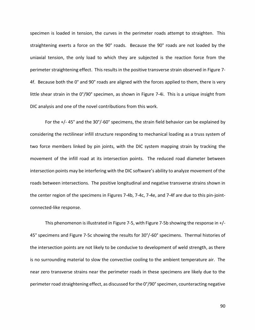
90
specimen is loaded in tension, the curves in the perimeter roads attempt to straighten. This
straightening exerts a force on the 90° roads. Because the 90° roads are not loaded by the
uniaxial tension, the only load to which they are subjected is the reaction force from the
perimeter straightening effect. This results in the positive transverse strain observed in Figure 7-
4f. Because both the 0° and 90° roads are aligned with the forces applied to them, there is very
little shear strain in the 0°/90° specimen, as shown in Figure 7-4i. This is a unique insight from
DIC analysis and one of the novel contributions from this work.
For the +/- 45° and the 30°/-60° specimens, the strain field behavior can be explained by
considering the rectilinear infill structure responding to mechanical loading as a truss system of
two force members linked by pin joints, with the DIC system mapping strain by tracking the
movement of the infill road at its intersection points. The reduced road diameter between
intersection points may be interfering with the DIC software’s ability to analyze movement of the
roads between intersections. The positive longitudinal and negative transverse strains shown in
the center region of the specimens in Figures 7-4b, 7-4c, 7-4e, and 7-4f are due to this pin-joint-
connected-like response.
This phenomenon is illustrated in Figure 7-5, with Figure 7-5b showing the response in +/-
45° specimens and Figure 7-5c showing the results for 30°/-60° specimens. Thermal histories of
the intersection points are not likely to be conducive to development of weld strength, as there
is no surrounding material to slow the convective cooling to the ambient temperature air. The
near zero transverse strains near the perimeter roads in these specimens are likely due to the
perimeter road straightening effect, as discussed for the 0°/90° specimen, counteracting negative

91
strains in the truss-like structure. Local yielding within the infill roads near the perimeter could
be limiting the strain transfer to the interior of the specimen.
Figure 7-5: Pin-joint-connected truss structure model for the mechanical response of sparse rectilinear infill. (a) Shows how the structure would respond to a uniaxial load, (b) shows response in a +/- 45° infill specimen, and (c) shows response in a 30°/-60° infill specimen.
The disparity in shear fields between the +/- 45° and the 30°/-60° specimens can also be
explained by this new insight. Any relative movement that is aligned with the X and Y axes of the
image would not be reported as shear strain. If the +/- 45° infill is deforming as illustrated in
Figure 7-5b, then any measurable shear strains would be very small. This matches with what was
observed in the shear strain field in Figure 7-4g. In the 30°/-60° specimens, this deformation
would not be aligned with the image X and Y axes and therefore the measured shear strains
would be larger in this case. The shear strain field shown in Figure 7-4h reflects what would be
expected with this behavior.

92
7.2.3 – Hexagonal Infill, 25% Density
The hexagonal infill specimen outperformed the rectilinear infill in 𝜎𝑒𝑓𝑓 at yield. The 0°
specimens were strongest and exhibited the most uniform strain fields, as shown in Figure 7-6.
This is likely because the 0° specimens are the only one to include toolpaths aligned with the
loading direction. The near-zero shear strains shown throughout the specimen (see Figure 7-6i),
indicate that most of the deformation occurrs in these toolpaths aligned with the applied load.
Similar to the rectilinear specimens, transverse strains near the perimeter are mitigated by the
perimeter straightening effect.
Figure 7-6: Full-field strain images of strain in the (a-c) loading direction, (d-f) transverse direction, and (g-i) shear strain at yield for the hexagonal infill 25% infill density with the primary (a,d,g) 0°, (b,e,h) 15°, and (c,f,i) 30° toolpath orientations.
As with the rectilinear specimens, strain localizations can be seen in the gage-to-grip
region transitions. Many of the hexagonal specimens exhibited grip failures, including all three
of the 0° specimens. The area exhibiting low strains near the upper grip that is not reflected in
the lower grip transition in the 15° specimen shown in Figure 7-6b is also likely due to the

93
specimen geometry. Similar to the rectilinear specimens, areas of higher strain can be seen in
the hexagonal specimen along the perimeter roads where there was no material deposited while
building the infill. These areas of higher strain can be seen in each of the three hexagonal
specimens, but they are more clearly visible in the 15° and 30° specimen in Figures 7-6b and 7-
6a.
Each of the strain fields in Figure 7-6 appear less uniform than those of the rectilinear 25%
infill density specimens. Because material is only deposited directly onto previously deposited
material in hexagonal infill, the infill roads are not drawn down to a smaller diameter. This extra
width appears to give the DIC software enough area to track strains within the individual infill
roads, rather than only between intersection points.
Full-field strain measurements of both the rectilinear and hexagonal sparse infill
geometries revealed some unexpected results. The pin-joint-like response of the rectilinear infill
suggests that this infill does little to resist deformation. The areas of increased strain along the
perimeter of the MEAM parts in both the rectilinear and hexagonal infill specimens is another
unexpected result. Failure initiated at these locations in all of the sparse specimen that were
tested. Eliminating these areas of increased strain is important when designing new infill
geometries that would optimize mechanical performance. The next section proposes such a new
infill geometry based on this result and compares its mechanical performance to these results.
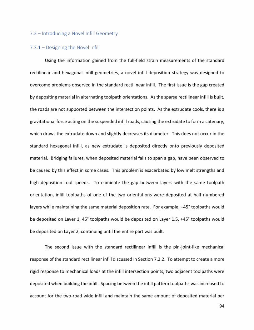
94
7.3 – Introducing a Novel Infill Geometry
7.3.1 – Designing the Novel Infill
Using the information gained from the full-field strain measurements of the standard
rectilinear and hexagonal infill geometries, a novel infill deposition strategy was designed to
overcome problems observed in the standard rectilinear infill. The first issue is the gap created
by depositing material in alternating toolpath orientations. As the sparse rectilinear infill is built,
the roads are not supported between the intersection points. As the extrudate cools, there is a
gravitational force acting on the suspended infill roads, causing the extrudate to form a catenary,
which draws the extrudate down and slightly decreases its diameter. This does not occur in the
standard hexagonal infill, as new extrudate is deposited directly onto previously deposited
material. Bridging failures, when deposited material fails to span a gap, have been observed to
be caused by this effect in some cases. This problem is exacerbated by low melt strengths and
high deposition tool speeds. To eliminate the gap between layers with the same toolpath
orientation, infill toolpaths of one of the two orientations were deposited at half numbered
layers while maintaining the same material deposition rate. For example, +45° toolpaths would
be deposited on Layer 1, 45° toolpaths would be deposited on Layer 1.5, +45° toolpaths would
be deposited on Layer 2, continuing until the entire part was built.
The second issue with the standard rectilinear infill is the pin-joint-like mechanical
response of the standard rectilinear infill discussed in Section 7.2.2. To attempt to create a more
rigid response to mechanical loads at the infill intersection points, two adjacent toolpaths were
deposited when building the infill. Spacing between the infill pattern toolpaths was increased to
account for the two-road wide infill and maintain the same amount of deposited material per

95
unit volume. The right side of Figure 7-7 shows the unit cell for this new linear infill type. Figure
7-8 illustrates the half-layer offset infill structure.
Figure 7-7: Toolpaths used to create hexagonal infill part and a 3D representation of the sparse rectilinear unit cell. Perimeter toolpaths are shown in black and infill toolpaths are shown in blue and green.
Figure 7-8: An illustration of the half-layer offset build strategy used in the new linear infill.
The third issue to be addressed in the standard rectilinear infill is the increased local
strains along the perimeter roads, as is discussed in Section 7.2.2. With the new infill pattern,
material is deposited in areas along the perimeter that remain open after infill deposition in an

96
attempt to create a more uniform mechanical response. The toolpaths used to deposit material
along the perimeter are shown in green on the left side of Figure 7-7.
7.3.2 – Mechanical Testing
The proposed linear infill specimens were strongest of any of the infill build strategies
tested. The 0°/90° specimens were strongest of all of the 25% infill density specimens tested.
The +/- 45° specimens were the strongest of any set that did not include toolpaths aligned with
the loading direction. Each one of these specimens failed at the grip-to-gage region transition.
At these failure points, failure appears to have initiated at the road intersection points. The half-
layer stagger at these interfaces appears to have introduced a stress concentration. However,
depositing two roads adjacent to one another and filling gaps in the infill at the infill-perimeter
interface has provided additional strength in these novel infill specimens.
Examining the strain fields in Figure 7-9, the 0°/90° specimens exhibited strain field trends
similar to the other 0°/90° build strategies. Strains in the loading direction are only present in
the 0° toolpath roads. Small positive transverse strains are seen in the 90° roads. The adjacent
0° roads form a wide enough structure for the DIC software to measure small negative strains in
these areas. Shear strains are near zero, in the new novel infill, which is as expected for this
toolpath orientation.

97
Figure 7-9: Full-field strain images of strain in the (a,b) loading direction, (c,d) transverse direction, and (e,f) shear strain at yield for the proposed linear infill 25% infill density with the (a,c,e) +/- 45° and (b,d,f) 0°/90° toolpath orientations.
In the +/- 45° specimen shown in Figure 7-9, the strain fields do differ from the other
linear toolpath specimens. In the loading direction strain field, shown in Figure 7-9a, strains are
near zero at the toolpath road intersections. In the other infill build strategy specimen, the DIC
software was tracking the movement of the intersection points relative to each other; thus, a
positive strain was seen in this region. In this case, the intersections are far enough apart that
the displacement of these locations evaluated independenly by the DIC software. Within each
intersection, the adjacent roads form a large enough surface area to calculate strains within the
infill roads. In the loading direction, there is very little strain at the intersections. The transverse
strain field shows a similar pattern to the other linear build strategies, with negative strains at
the center and near-zero strains along the perimeter.

98
The largest difference between the other linear infill build strategies and the novel linear
infill is seen in the shear strain field, shown in Figure 7-9e. Here, shear strains near zero can be
seen away from the intersection points. However, at the intersection points, shear strain can be
observed both within the infill and at the infill-perimeter interface. The weld interface between
the two adjacent toolpath roads does not allow the adjacent roads to move independently. This
lack of independent movement prevents the intersection points from acting like pin joints in a
truss structure. The positive shear strains at the interior intersection points and negative shear
strains at the infill-perimeter interface both show what would be expected of a connection that
has torsional stiffness.
7.4 – Summary of Results
Measuring the full-field strain of MEAM parts revealed several interesting results. Before
the onset of plastic deformation, the solid infill specimens respond to tensile deformation similar
to how solid materials are respond to the same loading condition. With this information,
engineers and designers can apply design rules developed for conventionally manufactured parts
to MEAM parts, so long as the design limits loading of the MEAM part to elastic deformation. As
peak force is reached, areas of increased strain appear at the weld interfaces within the gage
region of the solid infill specimens. These areas of locally increased strain centered on a weld
interface indicate that the weld interface is the location where the onset of part failure occurs.
The part strength calculation method presented in Section 5.1, which follows a weld interface
centric approach, is validated with this information.

99
The sparse infill specimen measurements provided new and interesting results. Areas of
locally increased strain along the perimeter of the MEAM parts in both the rectilinear and
hexagonal infill specimens was not expected. As failure was initiated in these areas of locally
increased strains, efforts to propose a novel infill deposition strategy as discussed in Section 7.3
to create a more uniform strain distribution.
Figure 7-10 is an Ashby-type plot comparing the tensile strength and build time of each
of the sparse infill geometry types. This plot clearly shows the key advantages of the novel infill
geometry introduced in this study. While the hexagonal infill outperforms the standard linear
infill, the large number of changes in toolpath direction result in long build times. The proposed
infill geometry offers the strength advantages of hexagonal infill, while maintaining the faster
build time of the rectilinear infill. While further testing is required, the novel infill geometry may
be a good candidate for default toolpaths in slicing algorithms for MEAM parts.

100
Figure 7-10: Ashby-type plot comparing effective ultimate tensile stress to build time of the 25% Infill Density specimens. Experimental data are shown as points. Dashed lines are used to encapsulate all data for one infill type.
101
8 – Contributions and Future Work
8.1 – Summary of Contributions
Based in the research results presented in this dissertation, designers and engineers can
make better informed decisions when designing parts for MEAM production. Ultimately, the
overarching goal in this work is to help MEAM become a viable a manufacturing process, not only
for fabricating prototypes but also for end-use parts. Engineers can use the new insights and
knowledge presented on the mechanical strength of MEAM parts to gain the confidence in the
process and design end-use parts using MEAM.
The new theory for estimating strength of a thermoplastic polymer weld presented in
Chapter 4 provides an accurate representation of how strength is developed at the weld interface
in MEAM parts. This theory was developed specifically for this purpose, with consideration given
to the unique qualities of welding two as-extruded surfaces. When applied to the weld interface
geometry and thermal history, as discussed in Chapter 5, accurate part strength predictions were
made using this weld strength theory. Comparisons with experimental strength values across
multiple polymetric materials were all within 7% of the value predicted by the theory, and some
strength predictions were within 1% of the experimental values, indicating accurate results.
Chapter 6 and 7 investigate effects of changes in build strategy on the mechanical
properties of MEAM parts based on this new theory. Experiments presented in Chapter 6 show
that just by changing material deposition strategy, which can be influenced by part geometry,
mechanical properties of the as-built MEAM part will change. This change is independent of the
process parameters used to build the part, as process parameters were held constant across all
102
experiments. The results of these experiments show that discontinuities do have a large effect
on part strength and suggest that the way mechanical properties are reported for MEAM parts is
questionable and may need to be revisited. Since build discontinuities can be induced by part
geometry, the actual strength of a part may be less than the reported strength for that material
and process combination. The materials testing procedure for MEAM fabricated parts needs to
be updated to account for the impact of build discontinuities. The reported mechanical
properties must reflect how MEAM parts will perform under real-world production and end-use
conditions, not idealized conditions that only exist in a laboratory setting.
Chapter 7 discussed the deformation that occurs within MEAM parts, and full-field strain
measurements were used to investigate the nature of this deformation. The solid infill geometry
parts, which are typically used when the part requires the most strength, behaved like solid
structures during elastic deformation. This is good news for engineers and designers, as they can
apply design rules developed for conventionally manufactured parts to MEAM parts, so long as
the design limits loading of the MEAM part to elastic deformation.
Full-field deformation results of the sparse infill specimen revealed flaws in the infill
deposition process. A novel infill geometry was introduced to address these flaws. This novel
infill geometry outperformed the standard rectilinear and hexagonal infill geometries, providing
symmetric strain distributions while maintaining the short build time of standard rectilinear infill.
This novel infill geometry should be considered a first option for engineers planning on building
MEAM parts with a sparse internal structure.

103
When applying this new knowledge to part design, designers and engineers can optimize
the geometry of the part, and the MEAM process used to produce the part, for their specific use-
cases. With knowledge on how strength is developed at the weld interfaces within the MEAM
part, how material deposition strategy effects part strength, and how the part will deform under
load, the engineer can be confident in how the part will perform during use. Using this
knowledge, MEAM can be viewed as a manufacturing process for end-use parts, not just a
prototyping tool.
8.2 – Limitations of the Research
The weld theory presented in Chapter 4 and used to estimate MEAM part strength in
Chapter 5 is only known to be valid for amorphous thermoplastic polymers. Semi-crystalline
polymers and amorphous polymers that serve as matrix for a composite material were not
considered when deriving and testing the presented theory for weld strength. It is unknown how
polymer crystal nucleation and growth effect molecular movement at thermoplastic polymer
weld interfaces. Filler materials may also influence how quickly polymer molecules can form
weld interface-spanning entanglements. Filler material geometry is known to have an effect on
viscosity in an MEAM process [8], and the MEAM process is known to cause alignment of the
filler material within the deposited extrudate [10]. It is unknown how these factors will affect
the weld interface in MEAM parts. Any changes to the rate of molecular diffusion would change
the rate of weld strength development. Additional terms would likely needed to be added to
Equation 4-1 to account for changes in the rate of diffusion due to the presence of polymer

104
crystals and/or filler materials and mechanical testing would be required to validate these
changes.
The strength predictions made and tested in Chapter 5 were only for one loading
condition: uniaxial tension. Additional factors may need to be considered when determining part
strength. For example, in the tensile tests, the grips used to hold the specimen loaded the infill
toolpaths directly. In an end-use part, loads might be applied to parts by bolts passing through
holes in the part. The interaction of the infill toolpaths and the perimeter toolpaths around the
hole may be the limiting factor in part strength. Loads in this bolt-in-hole condition may not be
as uniformly applied as the loads in the uniaxial tension experiments. Further testing of multiple
loading conditions, including compression and bending, is necessary.
Similarly, the full-field strain measurements discussed in Chapter 7 only describe the
response of MEAM parts to uniaxial tensile force. The response of MEAM parts to compression
or bending might be much different. Compression and bending tests may reveal that the solid
infill geometry parts, which responded to tensile deformation in a manner similar to solid parts
produced using conventional manufacturing processes, respond differently to the different
loading conditions. If this is the case, new design rules will need to be made for engineers and
designers to use MEAM parts in these loading conditions.
8.3 – Suggestions for Future Work
The new strength theory is well suited for use in MEAM build simulation software. A build
simulation that estimates the thermal history for each weld interface in the MEAM part using the

105
gcode used to build the part would be a powerful tool for designers and engineers. Engineers
would be able to iterate on their designs and modify toolpaths to optimize the part and customize
the MEAM manufacturing process for each part and use-case. Ultimately, a closed-loop
simulation could be created where both the part design and its associated toolpaths would be
optimized digitally.
Further study on the weld theory and part strength predictions is also needed. The work
presented in this document only represents tensile loading of MEAM parts. Further experiments
into other loading conditions, such as compression and bending are necessary. This work also
only studies straight-line weld interfaces. MEAM has the ability to produce complex geometry
parts, and weld interfaces within these parts may not always be straight lines. Applying this
strength theory to additional interface geometries and loading conditions is necessary work.
Testing the weld theory in Big Area Additive Manufacturing (BAAM) would be particularly
interesting. BAAM is a material extrusion process with incredibly large build volumes, up to 27
m3. These large build volumes create thermal histories that are much different than those seen
in the smaller scale MEAM machines. As the materials used in BAAM are the same as MEAM,
just with much higher volumetric deposition rates, the proposed part strength theory can be
applicable to BAAM parts. The change in processing conditions would provide a good test for the
validity of the presented theory.
Future experiments on weld interfaces of multiple materials is also necessary. Because
material is selectively deposited in MEAM processes, parts can be built using multiple
thermoplastic polymers. Understanding how these different polymers interact at the weld

106
interface is necessary for understanding how multi-material MEAM parts respond to mechanical
loads. This would likely require adding a term including the Flory-Huggins interaction parameter
[26] to equation 4-1. Understanding how these multi-material weld interfaces behave would
open the MEAM design space to include parts built using multiple thermoplastic polymers.
The full-field strain measurement study needs to be expanded upon to include multiple
loading conditions. In real-world applications, MEAM parts will not only see tensile loads.
Understanding how the internal lattice structure of sparse infill geometry MEAM parts responds
to bending and compression, particularly measuring when buckling would occur within the infill
structure, is necessary to fully understand how MEAM parts behave. Testing the response of
MEAM parts with solid and sparse infill geometries in compression and bending is a necessary
experiment.

107
References
[1] T. Wohlers, “3D Printing and Additive Manufacturing State of the Industry,” in Wohlers Report 2017, 2017.
[2] Sean Monahan, C. Chen, T. W. Simpson, and L. Taylor-Kale, “3D Printing and the Future of the US Economy,” 2017.
[3] Sean Monahan, “3-D printing’s economic benefits are too big to ignore | TheHill,” thehill.com, 2018.
[4] America Makes & ANSI Additive Manufacturing Standardization Collaboritive (AMSC), “Standardization Roadmap for Additive Manufacturing Version 2.0,” 2018.
[5] ISO/ASTM, ISO/ASTM 52900-2015: Additive manufacturing -- General principles -- Terminology. 2015.
[6] J. B. Khurana, S. Dinda, and T. W. Simpson, “Active-Z Printing: A New Approach to Increasing 3D Printed Part Strength,” 2017, pp. 1627–1642.
[7] I. Gibson, D. W. Rosen, and B. Stucker, Additive manufacturing technologies: Rapid prototyping to direct digital manufacturing. 2010.
[8] B. G. Compton and J. A. Lewis, “3D-printing of lightweight cellular composites,” Adv. Mater., 2014.
[9] N. Ashrafi, J. Duarte, S. Nazarian, and N. A. Meisel, “Evaluating the Relationship between Deposition and Layer Quality in Large-scale Additive Manufacturing of Concrete,” 2018.
[10] C. E. Bakis, R. T. Haluza, J. Bartolai, J. J. Kim, and T. W. Simpson, “Anisotropic Mechanical Properties of 3D Printed Carbon Whisker Reinforced PLA Composite Material,” Adv. Compos. Mater., 2018. Under Review.
[11] Markforged, “Materials: Metals.” [Online]. Available: https://markforged.com/materials/#metal. [Accessed: 01-Oct-2018].
[12] FlashForge, “FlashForge Finder Technical Specifications.” [Online]. Available: http://www.flashforge.com/finder-3d-printer/tech-specs/. [Accessed: 30-Sep-2018].
[13] C. E. Duty et al., “Structure and mechanical behavior of Big Area Additive Manufacturing (BAAM) materials,” Rapid Prototyp. J., 2017.
[14] C. McIlroy and P. D. Olmsted, “Disentanglement effects on welding behaviour of polymer melts during the fused-filament-fabrication method for additive manufacturing,” Polym. (United Kingdom), 2017.
[15] C. S. Davis, K. E. Hillgartner, S. H. Han, and J. E. Seppala, “Mechanical strength of welding zones produced by polymer extrusion additive manufacturing,” Addit. Manuf., 2017.
[16] J. E. Seppala, S. Hoon Han, K. E. Hillgartner, C. S. Davis, and K. B. Migler, “Weld formation during material extrusion additive manufacturing,” Soft Matter, 2017.
[17] J. Bartolai, T. W. Simpson, and R. Xie, “Predicting strength of additively manufactured thermoplastic polymer parts produced using material extrusion,” Rapid Prototyp. J., 2018.
[18] S. H. Ahn, C. Baek, S. Lee, and I. S. Ahn, “Anisotropic Tensile Failure Model of Rapid Prototyping Parts - Fused Deposition Modeling (FDM),” Int. J. Mod. Phys. B, vol. 17, no. 08n09, pp. 1510–1516, 2003.
[19] S.-H. Ahn, M. Montero, D. Odell, S. Roundy, and P. K. Wright, “Anisotropic material

108
properties of fused deposition modeling ABS,” Rapid Prototyp. J., vol. 8, no. 4, pp. 248–257, 2002.
[20] M. W. M. Cunico, “Analytical and experimental characterization of anisotropic mechanical behaviour of infill building strategies for fused deposition modelling objects,” 2017, pp. 984–991.
[21] M. Montero, S. Roundy, and D. Odell, “Material characterization of fused deposition modeling (FDM) ABS by designed experiments,” Proc. Rapid Prototyp. Manuf. Conf., pp. 1–21, 2001.
[22] A. K. Ravi, A. Deshpande, and K. H. Hsu, “An in-process laser localized pre-deposition heating approach to inter-layer bond strengthening in extrusion based polymer additive manufacturing,” J. Manuf. Process., 2016.
[23] Q. Sun, G. M. Rizvi, C. T. Bellehumeur, and P. Gu, “Effect of processing conditions on the bonding quality of FDM polymer filaments,” Rapid Prototyp. J., vol. 14, no. 2, pp. 72–80, 2008.
[24] D. Grewell and A. Benatar, “Welding of plastics: Fundamentals and new developments,” in International Polymer Processing, 2007, vol. 22, no. 1, pp. 43–60.
[25] R. P. Wool and K. M. O’Connor, “A theory of crack healing in polymers,” J. Appl. Phys., vol. 52, no. 10, pp. 5953–5963, 1981.
[26] M. Rubinstein and R. H. Colby, “Polymer physics,” Polymer International. 2003. [27] F. Yang and R. Pitchumani, “Healing of thermoplastic polymers at an interface under
nonisothermal conditions,” Macromolecules, vol. 35, no. 8, pp. 3213–3224, 2002. [28] M. Doi and S. Edwards, “The Theory of Polymer Dynamics,” … University Press. 1986. [29] R. P. Wool, B. L. Yuan, and O. J. McGarel, “Welding of polymer interfaces,” Polym. Eng.
Sci., vol. 29, no. 19, pp. 1340–1367, 1989. [30] O. a Ezekoye, C. D. Lowman, M. T. Fahey, and a G. Hulme-Lowe, “Polymer weld strength
predictions using a thermal and polymer chain diffusion analysis,” Polym. Eng. Sci., vol. 38, no. 6, pp. 976–991, 1998.
[31] L. J. Bastien and J. W. Gillespie, “A non-isothermal healing model for strength and toughness of fusion bonded joints of amorphous thermoplastics,” Polym. Eng. Sci., vol. 31, no. 24, pp. 1720–1730, 1991.
[32] P. E. J. Rouse, “A Theory of the Linear Viscoelastic Properties of Dilute Solutions of Coiling Polymers,” J. Chem. Phys., 1953.
[33] M. Doi, Introduction to polymer physics. 1996. [34] M. L. Williams, R. F. Landel, and J. D. Ferry, “The Temperature Dependence of Relaxation
Mechanisms in Amorphous Polymers and Other Glass-forming Liquids1,” J. Am. Chem. Soc., vol. 77, no. 12, pp. 3701–3707, 1955.
[35] D. B. Kline and R. P. Wool, “Polymer welding relations investigated by a lap shear joint method,” Polym. Eng. Sci., vol. 28, no. 1, pp. 52–57, Jan. 1988.
[36] R. P. Wool, “Strength and Entanglement Development at Amorphous Polymer Interfaces,” in Amorphous Polymers and Non-Newtonian Fluids, C. Dafermos, J. L. Ericksen, and D. Kinderlehrer, Eds. New York, NY: Springer New York, 1987, pp. 169–187.
[37] J. E. Seppala and K. D. Migler, “Infrared thermography of welding zones produced by polymer extrusion additive manufacturing,” Addit. Manuf., vol. 12, pp. 71–76, 2016.
[38] T. J. Coogan and D. O. Kazmer, “Healing simulation for bond strength prediction of FDM,”
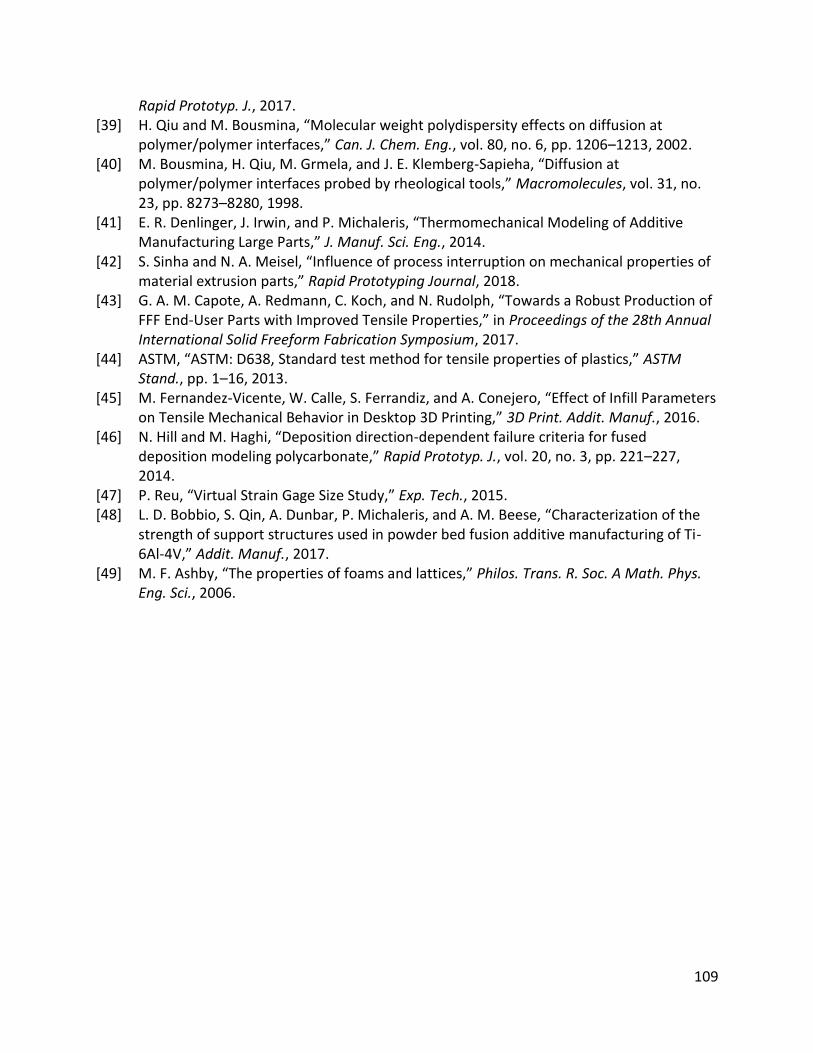
109
Rapid Prototyp. J., 2017. [39] H. Qiu and M. Bousmina, “Molecular weight polydispersity effects on diffusion at
polymer/polymer interfaces,” Can. J. Chem. Eng., vol. 80, no. 6, pp. 1206–1213, 2002. [40] M. Bousmina, H. Qiu, M. Grmela, and J. E. Klemberg-Sapieha, “Diffusion at
polymer/polymer interfaces probed by rheological tools,” Macromolecules, vol. 31, no. 23, pp. 8273–8280, 1998.
[41] E. R. Denlinger, J. Irwin, and P. Michaleris, “Thermomechanical Modeling of Additive Manufacturing Large Parts,” J. Manuf. Sci. Eng., 2014.
[42] S. Sinha and N. A. Meisel, “Influence of process interruption on mechanical properties of material extrusion parts,” Rapid Prototyping Journal, 2018.
[43] G. A. M. Capote, A. Redmann, C. Koch, and N. Rudolph, “Towards a Robust Production of FFF End-User Parts with Improved Tensile Properties,” in Proceedings of the 28th Annual International Solid Freeform Fabrication Symposium, 2017.
[44] ASTM, “ASTM: D638, Standard test method for tensile properties of plastics,” ASTM Stand., pp. 1–16, 2013.
[45] M. Fernandez-Vicente, W. Calle, S. Ferrandiz, and A. Conejero, “Effect of Infill Parameters on Tensile Mechanical Behavior in Desktop 3D Printing,” 3D Print. Addit. Manuf., 2016.
[46] N. Hill and M. Haghi, “Deposition direction-dependent failure criteria for fused deposition modeling polycarbonate,” Rapid Prototyp. J., vol. 20, no. 3, pp. 221–227, 2014.
[47] P. Reu, “Virtual Strain Gage Size Study,” Exp. Tech., 2015. [48] L. D. Bobbio, S. Qin, A. Dunbar, P. Michaleris, and A. M. Beese, “Characterization of the
strength of support structures used in powder bed fusion additive manufacturing of Ti-6Al-4V,” Addit. Manuf., 2017.
[49] M. F. Ashby, “The properties of foams and lattices,” Philos. Trans. R. Soc. A Math. Phys. Eng. Sci., 2006.

110
Appendix A – Materials and Methods
Table A-1: MEAM machine details.
Equipment Manufacturer Model
MEAM Machine Frame Maker’s Tool Works Mendel Max 3
Control Electronics UltiMachine RAMBo 1.3
Nozzle e3D Online e3D-v6
Temperature Measurement e3D Online v6 PT100
Power Supply MeanWell SE-350-24
Firmware Marlin Firmware Marlin 1.4.4
Table A-2: Material Supplier Information.
Material Supplier Feedstock Nominal Diameter
Acrylonitrile Butadiene
Styrene MakeShaper 2.85 mm
Polycarbonate GizmoDorks 2.85 mm
Table A-3: MEAM tensile specimen build process parameters.
Build Parameter ABS PC
Nozzle Temp. 230° C 285° C
Build Plate Temp. 115° C 150° C
Nozzle Travel Speed 60 mm/s 60 mm/s
Layer Height 0.2 mm 0.2 mm
Extrudate Width 0.4 mm 0.4 mm
Extrusion Factor [43] 1.02 1.04
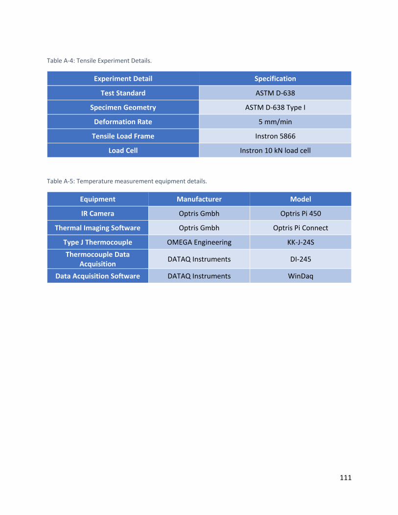
111
Table A-4: Tensile Experiment Details.
Experiment Detail Specification
Test Standard ASTM D-638
Specimen Geometry ASTM D-638 Type I
Deformation Rate 5 mm/min
Tensile Load Frame Instron 5866
Load Cell Instron 10 kN load cell
Table A-5: Temperature measurement equipment details.
Equipment Manufacturer Model
IR Camera Optris Gmbh Optris Pi 450
Thermal Imaging Software Optris Gmbh Optris Pi Connect
Type J Thermocouple OMEGA Engineering KK-J-24S
Thermocouple Data Acquisition
DATAQ Instruments DI-245
Data Acquisition Software DATAQ Instruments WinDaq

112
Appendix B – Weld interface thermal history plots
Figure B-1: Weld interface thermal history of a +/- 45° infill toolpath orientation PC tensile specimen.

113
Figure B-2: Weld interface thermal history of a +/- 45° infill toolpath orientation continuous build ABS tensile specimen.
Figure B-3: Weld interface thermal history of a +/- 45° infill toolpath orientation discontinuous build ABS tensile specimen.

114
Figure B-4: Weld interface thermal history of a 90° infill toolpath orientation continuous build ABS tensile specimen.
Figure B-5: Weld interface thermal history of a 90° infill toolpath orientation discontinuous build ABS tensile specimen.

115
Figure B-6: Weld interface thermal history of a 0°/90° infill toolpath orientation continuous build ABS tensile specimen.
Figure B-7: Weld interface thermal history of a 0°/90° infill toolpath orientation discontinuous build ABS tensile specimen.

116
Figure B-8: Weld interface thermal history of a +/- 30° infill toolpath orientation continuous build ABS tensile specimen.
Figure B-9: Weld interface thermal history of a +/- 30° infill toolpath orientation discontinuous build ABS tensile specimen.

117
Appendix C – Fracture Surface Images
Figure C-1: Fracture surface of a +/- 45° toolpath orientation continuous build PC tensile specimen.
Figure C-2: Fracture surface of a +/- 45° toolpath orientation continuous build ABS tensile specimen.

118
Figure C-3: Fracture surface of a +/- 45° toolpath orientation discontinuous build ABS tensile specimen.
Figure C-4: Fracture surface of a 90° toolpath orientation continuous build ABS tensile specimen.

119
Figure C-5: Fracture surface of a 90° toolpath orientation discontinuous build ABS tensile specimen.
Figure C-6: Fracture surface of a +/- 30° toolpath orientation continuous build ABS tensile specimen.

120
Figure C-7: Fracture surface of a +/- 30° toolpath orientation discontinuous build ABS tensile specimen.

121
Appendix D – MEAM part strength calculation parameters
Table D-1: Area Measurements used in tensile specimen strength calculations.
Specimen Type Atotal Aweld,layer Aper,layer Ainfill,layer
PC - ± 45° Continuous
41.6 mm2 1.92 mm2 0.319 mm2 2.26 mm2
ABS - ± 45° Continuous
41.6 mm2 2.03 mm2 0.314 mm2 2.20 mm2
ABS - 45° Discontinuous
41.6 mm2 2.03 mm2 0.314 mm2 2.20 mm2
ABS - 90° Continuous
41.6 mm2 1.64 mm2 0.317 mm2 2.54 mm2
ABS - 90° Discontinuous
41.6 mm2 1.44 mm2 0.317 mm2 2.54 mm2
ABS - 0°/90° Continuous
41.6 mm2 1.64 mm2 0.317 mm2 2.54 mm2
ABS - 0°/90° Discontinuous
41.6 mm2 1.44 mm2 0.317 mm2 2.54 mm2
ABS - ± 30° Continuous
41.6 mm2 2.87 mm2 0.314 mm2 2.11 mm2
ABS - ± 30° Discontinuous
41.6 mm2 2.87 mm2 0.314 mm2 2.11 mm2

122
Table D-2: Weld strength and layer strength values for PC +/- 45° continuous tensile specimen strength calculations.
Layer Number 𝝈𝒘 𝑭𝒍𝒂𝒚𝒆𝒓,𝒘𝒆𝒍𝒅 𝑭𝒍𝒂𝒚𝒆𝒓,𝒎𝒂𝒙
1 65.4 MPa 146.3 N 168.6 N
2 65.4 MPa 146.3 N 168.6 N
3 65.4 MPa 146.3 N 168.6 N
4 65.4 MPa 146.3 N 168.6 N
5 65.4 MPa 146.3 N 168.6 N
6 65.4 MPa 146.3 N 168.6 N
7 65.4 MPa 146.3 N 168.6 N
8 65.4 MPa 146.3 N 168.6 N
9 65.4 MPa 146.3 N 168.6 N
10 65.4 MPa 146.3 N 168.6 N
11 65.4 MPa 146.3 N 168.6 N
12 65.4 MPa 146.3 N 168.6 N
13 65.4 MPa 146.3 N 168.6 N
14 65.4 MPa 146.3 N 168.6 N
15 65.4 MPa 146.3 N 168.6 N
16 65.4 MPa 146.3 N 168.6 N

123
Table D-3: Weld strength and layer strength values for ABS +/- 45° continuous tensile specimen strength calculations.
Layer Number 𝝈𝒘 𝑭𝒍𝒂𝒚𝒆𝒓,𝒘𝒆𝒍𝒅 𝑭𝒍𝒂𝒚𝒆𝒓,𝒎𝒂𝒙
1 43.0 MPa 100.9 N 108.0 N
2 43.0 MPa 100.9 N 108.0 N
3 43.0 MPa 100.9 N 108.0 N
4 43.0 MPa 100.9 N 108.0 N
5 43.0 MPa 100.9 N 108.0 N
6 43.0 MPa 100.9 N 108.0 N
7 43.0 MPa 100.9 N 108.0 N
8 43.0 MPa 100.9 N 108.0 N
9 43.0 MPa 100.9 N 108.0 N
10 43.0 MPa 100.9 N 108.0 N
11 43.0 MPa 100.9 N 108.0 N
12 43.0 MPa 100.9 N 108.0 N
13 42.99 MPa 100.9 N 108.0 N
14 42.99 MPa 100.9 N 108.0 N
15 42.98 MPa 100.8 N 108.0 N
16 42.25 MPa 99.3 N 108.0 N

124
Table D-4: Weld strength and layer strength values for ABS +/- 45° discontinuous tensile specimen strength calculations.
Layer Number 𝝈𝒘 𝑭𝒍𝒂𝒚𝒆𝒓,𝒘𝒆𝒍𝒅 𝑭𝒍𝒂𝒚𝒆𝒓,𝒎𝒂𝒙
1 43.0 MPa 100.9 N 108.0 N
2 43.0 MPa 100.9 N 108.0 N
3 43.0 MPa 100.9 N 108.0 N
4 43.0 MPa 100.9 N 108.0 N
5 43.0 MPa 100.9 N 108.0 N
6 43.0 MPa 100.9 N 108.0 N
7 43.0 MPa 100.9 N 108.0 N
8 43.0 MPa 100.9 N 108.0 N
9 43.0 MPa 100.9 N 108.0 N
10 43.0 MPa 100.9 N 108.0 N
11 43.0 MPa 100.9 N 108.0 N
12 42.99 MPa 100.9 N 108.0 N
13 42.99 MPa 100.9 N 108.0 N
14 42.98 MPa 100.8 N 108.0 N
15 42.8 MPa 100.4 N 108.0 N
16 9.14 MPa 32.1 N 108.0 N

125
Table D-5: Weld strength and layer strength values for ABS 90° continuous tensile specimen strength calculations.
Layer Number 𝝈𝒘 𝑭𝒍𝒂𝒚𝒆𝒓,𝒘𝒆𝒍𝒅 𝑭𝒍𝒂𝒚𝒆𝒓,𝒎𝒂𝒙
1 42.98 MPa 84.22 N 110.9 N
2 42.98 MPa 84.22 N 110.9 N
3 42.98 MPa 84.22 N 110.9 N
4 42.98 MPa 84.22 N 110.9 N
5 42.98 MPa 84.22 N 110.9 N
6 42.98 MPa 84.22 N 110.9 N
7 42.98 MPa 84.22 N 110.9 N
8 42.98 MPa 84.22 N 110.9 N
9 42.98 MPa 84.22 N 110.9 N
10 42.98 MPa 84.22 N 110.9 N
11 42.98 MPa 84.22 N 110.9 N
12 42.98 MPa 84.22 N 110.9 N
13 42.97 MPa 84.21 N 110.9 N
14 42.91 MPa 84.09 N 110.9 N
15 42.61 MPa 83.60 N 110.9 N
16 39.75 MPa 78.91 N 110.9 N

126
Table D-6: Weld strength and layer strength values for ABS 90° discontinuous tensile specimen strength calculations.
Layer Number 𝝈𝒘 𝑭𝒍𝒂𝒚𝒆𝒓,𝒘𝒆𝒍𝒅 𝑭𝒍𝒂𝒚𝒆𝒓,𝒎𝒂𝒙
1 39.16 MPa 69.90 N 110.9 N
2 39.16 MPa 69.90 N 110.9 N
3 39.16 MPa 69.90 N 110.9 N
4 39.16 MPa 69.90 N 110.9 N
5 39.16 MPa 69.90 N 110.9 N
6 39.16 MPa 69.90 N 110.9 N
7 39.16 MPa 69.90 N 110.9 N
8 39.16 MPa 69.90 N 110.9 N
9 39.16 MPa 69.90 N 110.9 N
10 39.16 MPa 69.90 N 110.9 N
11 39.16 MPa 69.90 N 110.9 N
12 38.86 MPa 69.44 N 110.9 N
13 37.85 MPa 68.03 N 110.9 N
14 36.42 MPa 65.97 N 110.9 N
15 23.57 MPa 60.44 N 110.9 N
16 9.91 MPa 27.89 N 110.9 N

127
Table D-7: Weld strength and layer strength values for ABS 0°/90° continuous tensile specimen strength calculations.
Layer Number 𝝈𝒘 𝑭𝒍𝒂𝒚𝒆𝒓,𝒘𝒆𝒍𝒅 𝑭𝒍𝒂𝒚𝒆𝒓,𝒎𝒂𝒙
1 N/A N/A 109.25 N
2 42.99 MPa 84.24 N 110.9 N
3 N/A N/A 109.25 N
4 42.99 MPa 84.24 N 110.9 N
5 N/A N/A 109.25 N
6 42.99 MPa 84.24 N 110.9 N
7 N/A N/A 109.25 N
8 42.99 MPa 84.24 N 110.9 N
9 N/A N/A 109.25 N
10 42.99 MPa 84.23 N 110.9 N
11 N/A N/A 109.25 N
12 42.97 MPa 84.19 N 110.9 N
13 N/A N/A 109.25 N
14 42.78 MPa 83.89 N 110.9 N
15 N/A N/A 109.25 N
16 39.75 MPa 78.91 N 110.9 N

128
Table D-6: Weld strength and layer strength values for ABS 0°/90° discontinuous tensile specimen strength calculations.
Layer Number 𝝈𝒘 𝑭𝒍𝒂𝒚𝒆𝒓,𝒘𝒆𝒍𝒅 𝑭𝒍𝒂𝒚𝒆𝒓,𝒎𝒂𝒙
1 N/A N/A 109.25 N
2 42.92 MPa 84.1124 N 110.9 N
3 N/A N/A 109.25 N
4 42.92 MPa 84.11 N 110.9 N
5 N/A N/A 109.25 N
6 42.84 MPa 83.99 N 110.9 N
7 N/A N/A 109.25 N
8 42.72 MPa 83.79 N 110.9 N
9 N/A N/A 109.25 N
10 42.37 MPa 83.22N 110.9 N
11 N/A N/A 109.25 N
12 41.11 MPa 81.14 N 110.9 N
13 N/A N/A 109.25 N
14 35.14 MPa 71.36 N 110.9 N
15 N/A N/A 109.25 N
16 4.50 MPa 21.05 N 110.9 N

129
Table D-7: Weld strength and layer strength values for ABS +/- 30° continuous tensile specimen strength calculations.
Layer Number 𝝈𝒘 𝑭𝒍𝒂𝒚𝒆𝒓,𝒘𝒆𝒍𝒅 𝑭𝒍𝒂𝒚𝒆𝒓,𝒎𝒂𝒙
1 43.0 MPa 137.0 N 104.4 N
2 43.0 MPa 137.0 N 104.4 N
3 43.0 MPa 137.0 N 104.4 N
4 43.0 MPa 137.0 N 104.4 N
5 43.0 MPa 137.0 N 104.4 N
6 43.0 MPa 137.0 N 104.4 N
7 43.0 MPa 137.0 N 104.4 N
8 43.0 MPa 137.0 N 104.4 N
9 43.0 MPa 137.0 N 104.4 N
10 43.0 MPa 137.0 N 104.4 N
11 43.0 MPa 137.0 N 104.4 N
12 43.0 MPa 137.0 N 104.4 N
13 43.0 MPa 137.0 N 104.4 N
14 42.99 MPa 137.0 N 104.4 N
15 42.98 MPa 137.0 N 104.4 N
16 42.46 MPa 135.5 N 104.4 N

130
Table D-8: Weld strength and layer strength values for ABS +/- 30° discontinuous tensile specimen strength calculations.
Layer Number 𝝈𝒘 𝑭𝒍𝒂𝒚𝒆𝒓,𝒘𝒆𝒍𝒅 𝑭𝒍𝒂𝒚𝒆𝒓,𝒎𝒂𝒙
1 43.0 MPa 137.0 N 104.4 N
2 43.0 MPa 137.0 N 104.4 N
3 43.0 MPa 137.0 N 104.4 N
4 43.0 MPa 137.0 N 104.4 N
5 43.0 MPa 137.0 N 104.4 N
6 43.0 MPa 137.0 N 104.4 N
7 43.0 MPa 137.0 N 104.4 N
8 43.0 MPa 137.0 N 104.4 N
9 43.0 MPa 137.0 N 104.4 N
10 43.0 MPa 137.0 N 104.4 N
11 43.0 MPa 137.0 N 104.4 N
12 43.0 MPa 137.0 N 104.4 N
13 42.99 MPa 137.0 N 104.4 N
14 42.99 MPa 137.0 N 104.4 N
15 42.90 MPa 136.8 N 104.4 N
16 25.89 MPa 87.91 N 104.4 N

VITA
Joseph Bartolai
Education Doctor of Philosophy in Mechanical Engineering December 2018 The Pennsylvania State University; University Park, PA, USA Master of Science in Mechanical Engineering December 2016 The Pennsylvania State University; University Park, PA, USA Bachelor of Science in Mechanical Engineering May 2013 The Pennsylvania State University; University Park, PA, USA
Work Experience Graduate Research Assistant Center for Innovative Materials Processing through Direct Digital Deposition (CIMP-3D) The Pennsylvania State University; University Park, PA, USA August 2014 – December 2018
• Developed novel theory for strength of thermoplastic parts produced by Material Extrusion Additive Manufacturing (MEAM)
• Developed a novel method for creating functionally graded material (FGM) interfaces using Triply Periodic Minimal Surfaces (TPMS)
• Evaluated candidate polymers for use in Additive Manufacturing by Material Extrusion
Graduate Teaching Assistant Department of Mechanical and Nuclear Engineering The Pennsylvania State University; University Park, PA, USA August 2014 – May 2015 January 2016 – May 2018
• Taught Laboratory Sections of Mechanical Engineering Design Methodology (5 Semesters)
• Developed laboratory class content for Mechanical Engineering Design Methodology
• Taught Vibrations Laboratory (2 Semesters)
Project Engineer – Regulatory Compliance Victaulic Company; Easton, PA, USA June 2013 – July 2014
• Developed Machinery Directive (2006/42/EC) compliance documentation and safety review procedures for pipe preparation tools
• Developed Technical Construction Files for Ball, Butterfly, and Check Valves along with Strainers and Suction Diffusers to validate Pressure Equipment Directive (97/23/EC) compliance
• Developed a correlation between ambient and elevated temperature mechanical properties of pressure boundary materials