Predator and Prey, Past, Present, and Projected: Modelling

Polar Bears and Ringed Seals in a Dynamic Arctic

by

Jody Renae Reimer

A thesis submitted in partial fulfillment of the requirements for the degree of

Doctor of Philosophy

in

Applied Mathematics

Departments of Mathematical and Statistical Sciences and Biological Sciences

University of Alberta

c⃝ Jody Renae Reimer, 2019

Abstract

Climate change is causing the Arctic to warm faster than anywhere else on earth. The

projected effects of a warmer Arctic include changes in population dynamics and distribu-

tions, biodiversity, food web structure, and ecosystem services. Our ability to successfully

monitor ecological changes and manage vulnerable populations relies on our ability to pre-

dict these responses. Mechanistic mathematical models are a powerful tool for exploring

the unprecedented nature of these environmental changes, allowing us to make quantitative,

testable predictions—a hallmark of scientific understanding—against which we can compare

future observations.

Unfortunately, we lack even baseline population estimates for many ice-associated species.

Polar bears and ringed seals, however, are two species for which we have data spanning

multiple decades, making them suitable indicator species for detecting broader ecological

change. There is a strong predator-prey relationship between polar bears and ringed seals,

and both species rely on the sea ice. Ringed seals rely on the sea ice, and the snow on top,

for moulting and for the creation of the protective snow lairs in which they give birth. Polar

bears rely on the sea ice for travel, mate finding, hunting, and, in some regions, for maternity

denning. Changes in the sea ice thus affect both species directly as well as indirectly through

their predator-prey relationship.

Historically, environmental conditions with negative effects on ringed seals and polar

bears came in the form of anomalously cold winters, resulting in heavier ice cover. In these

years, ringed seal reproductive rates declined, changing the prey availability for polar bears.

Due to climate change, however, these years of extreme cold are being replaced by years of

extreme heat. In the Beaufort Sea and Amundsen Gulf, Canada, this is resulting in earlier

spring sea ice breakup and a later autumn ice freezeup. This later freezeup results in reduced

snow accumulation on the ice, as the early winter snow falls on open water. For ringed seals,

their reliance on stable sea ice and sufficiently deep snow drifts in which to dig their spring

ii

birth lairs makes them vulnerable to these changes. For polar bears, earlier ice breakup

shortens the length of the important spring hunting season, with energetic consequences.

In this thesis, I explored the responses of ringed seals and polar bears to past, present,

and predicted environmental challenges. To do so, I used matrix population models and

stochastic dynamic programming (SDP). I found that polar bears typically strongly select

for ringed seal pups, but switch to disproportionately select older ringed seals in those years

with low pup availability corresponding to anomalously cold winters—a novel ecological

phenomenon I termed intraspecific prey switching. Looking ahead, I coupled a ringed seal

population model to ice and snow forecasts, modelling the population to the end of this

century. These projections showed median declines in population size of more than 50%, with

concurrent changes in population structure. Data collected through the current monitoring

program is not sufficient to detect these changes, highlighting the need to re-evaluate existing

field programs in light of emerging stressors. Anticipating the shorter spring feeding season,

I modelled shifts in a female polar bear’s optimal behavioural and physiological strategies

and the consequences for her expected lifetime reproductive output. This highlighted the

effect that seemingly small annual changes may have over the entire lifetime of a long-lived

species.

Additionally, the intuition developed through the application of matrix population models

in this thesis proved useful in understanding patterns which emerge in ecological applications

of SDP. A rich body of mathematical results on SDP exist, but have not been popularized

in the ecological SDP literature. I applied relevant mathematical results to two canonical

SDP equations in ecology, demonstrating their utility both for solving SDP models and for

interpreting their biological implications.

This thesis contributes to our understanding of Arctic marine ecology, provides exam-

ples of appropriate mathematical tools and interpretive paradigms with which to explore

ecological effects of climate change, and suggests new methods for applications of SDP in

ecology.

iii

Preface

Chapter 2 of this thesis has been published as: Reimer, J.R., Caswell, H., Derocher,

A.E., and Lewis, M.A. (2019). Ringed seal demography in a changing climate. Ecological

Applications. doi:10.1002/eap.1855. I conceived of the project, constructed and analyzed

the models, and wrote the manuscript. H. Caswell provided advice on model construction

and analysis. H. Caswell, A.E. Derocher, and M.A. Lewis provided supervisory guidance

and contributed to manuscript composition. Additionally, Amy Johnson created the map in

Figure 2.1 and David McGeachy obtained and processed the NSIDC sea ice data.

Chapter 3 has been published as: Reimer, J.R., Brown, H., Beltaos-Kerr, E., and de

Vries, G. (2018) Evidence of intraspecific prey switching: stage-structured predation of po-

lar bears on ringed seals. Oecologia, 189(1), 133-148. doi:10.1007/s00442-018-4297-x. I was

responsible for idea formulation, writing of the manuscript, and model analysis and inter-

pretation. All authors contributed to model design, interpretation of model results, and

provided editorial advice.

Chapter 4 is currently in review as: Reimer, J.R., Mangel, M., Derocher, A.E., and

Lewis, M.A. Modelling optimal responses and fitness consequences in a changing Arctic. I

designed, implemented, and analyzed the model, interpreted model results, and wrote the

manuscript. Supervisory guidance on all aspects of this project was provided by M. Mangel,

A.E. Derocher, and M.A. Lewis.

Chapter 5 is currently in review as: Reimer, J.R., Mangel, M., Derocher, A.E., and Lewis,

M.A. Matrix methods for stochastic dynamic programming in ecology and evolutionary

biology. I conceived of the project, which was enriched through discussion with the other

authors. I conducted all model analysis and wrote the manuscript, with editorial advice

from the other authors, who also provided supervisory guidance.

iv

Acknowledgments

I am grateful for the financial support that I received through an NSERC Vanier Canada

Graduate Scholarship, an Alberta Innovates Graduate Student Scholarship, and an Izaak

Walton Killam Memorial Scholarship. Additionally, the Michael Smith Foreign Study Sup-

plement funded my four month visit to the University of Amsterdam, where much of the

work in Chapter 2 was completed.

Discussions with Dr. Peter Molnar laid the conceptual groundwork for some of the ideas

in Chapter 4, and I have been grateful for his mentorship throughout. Dr. Thomas Hillen

had the astute observation, several years into my PhD, that a lot of what excited me was

motivated by biological questions rather than strictly mathematical ones, which caused me

to switch into the interdisciplinary program. Thank you, Thomas, for helping me explore

what drives me, and for your role on my supervisory committee.

Early in my degree, I had the opportunity to spend a week visiting Dr. Marc Mangel to

discuss stochastic dynamic programming applications in ecology. The foundations laid during

that week eventually grew into Chapters 4 and 5. I consider myself incredibly fortunate to

have stayed in contact with Marc throughout these past several years, and the clarity and

depth of this work has benefited from his involvement and mentorship. I am also grateful

for the warm welcome I received as a visiting student in Dr. Hal Caswell’s research group

at the University of Amsterdam. Those four months were both scientifically and personally

enriching, and a definite highlight.

Thank you to both the Lewis and Derocher labs, for all of your feedback on this work

and for being warm and supportive communities of which to be a part. To my colleagues

in applied math, with whom I completed my courses (especially Dean Koch and Carlos

Contreras), I cannot overstate how much I have appreciated your friendship, kindness, and

all of the hours spent working and laughing together.

I have been incredibly fortunate to spend these years testing my scientific wings under the

supervision of Drs. Mark Lewis and Andrew Derocher. Mark, it has been an honour to work

with you and to be part of your lab. We had many meetings over the years where I went in

feeling overwhelmed or directionless, but left feeling excited about my project and about the

next steps. I have appreciated the intentionality with which you run the lab, from discussing

broad scientific themes at lab retreats to weekly stimulating discussions in lab meetings. I

have learned so much from you about mathematical ecology and how to communicate to an

interdisciplinary audience. Thank you, Andy, for believing in a mathematician who did not

know the difference between a sea lion and a ringed seal when she showed up to work on

v

her PhD. I never imagined that I would get the opportunity to be out in the field collecting

samples from polar bears. Your patience explaining and re-explaining Arctic ecology to

me was remarkable. I have also learned so many unexpected skills from time spent in your

lab—from how to navigate the politics of working on a high profile species, to the importance

of not burying rejected manuscripts in a drawer forever. Thank you both for your scientific

mentorship, as well as guidance navigating grant applications, the murky rules of academic

etiquette, and, more recently, applying for postdoctoral positions.

I am so grateful for the support of my friends and family. Thanks to the women of the

cat house (Shawna, Lauren, and Janina) for 3 great years of laughter and living room yoga.

Wafa, Laura, Alice, Hannah, Beth, and Cassandra, your friendship throughout the years has

kept me sane and brought me so much joy. To my sisters, Krista and Vanessa, It has been

such a treat to see where a foundation in mathematics has taken all of us. To my parents,

Wes and Sherril, thank you for going on this adventure with me through all these years,

from Winnipeg, to Finland, to Oxford, and finally to Edmonton. I hope you will tolerate

this nomadic lifestyle for just a few more years and I promise one day I will buy a house and

take the piano out of your storage.

Finally, thank you to Seth Bryant, who tolerated my descriptions of the minutiae of life

in academia for longer than anyone should have to. Thank you for all of the things you do to

support me, even when I like to pretend that I don’t need support. Our shared experiences

and adventures during this degree have challenged and empowered me, helped keep the ups

and downs of a PhD in perspective, and added so much richness to my life.

vi

Table of Contents

1 Introduction 1

1.1 Arctic marine ecology . . . . . . . . . . . . . . . . . . . . . . . . . . . . . . . 1

1.1.1 Ringed seals and polar bears . . . . . . . . . . . . . . . . . . . . . . . 2

1.1.2 Climate change in the Arctic . . . . . . . . . . . . . . . . . . . . . . . 3

1.2 Mathematics of ringed seals and polar bears . . . . . . . . . . . . . . . . . . 5

1.2.1 Matrix population models . . . . . . . . . . . . . . . . . . . . . . . . 5

1.2.2 Stochastic dynamic programming . . . . . . . . . . . . . . . . . . . . 6

1.2.3 Shared foundations of nonnegative matrices . . . . . . . . . . . . . . 7

1.3 Thesis overview . . . . . . . . . . . . . . . . . . . . . . . . . . . . . . . . . . 7

2 Ringed seal demography in a changing climate 9

2.1 Introduction . . . . . . . . . . . . . . . . . . . . . . . . . . . . . . . . . . . . 9

2.1.1 Ringed seal populations, past and future . . . . . . . . . . . . . . . . 10

2.1.2 Geographic study area . . . . . . . . . . . . . . . . . . . . . . . . . . 13

2.1.3 Modelling overview . . . . . . . . . . . . . . . . . . . . . . . . . . . . 13

2.2 Materials and methods . . . . . . . . . . . . . . . . . . . . . . . . . . . . . . 14

2.2.1 Structured population model . . . . . . . . . . . . . . . . . . . . . . . 14

2.2.2 Linking reproduction to historical late ice breakup . . . . . . . . . . . 16

2.2.3 A note on parameter inconsistencies . . . . . . . . . . . . . . . . . . . 18

2.2.4 Linking pup survival to projected early ice breakup and reduced spring

snow depth . . . . . . . . . . . . . . . . . . . . . . . . . . . . . . . . 18

2.3 Results . . . . . . . . . . . . . . . . . . . . . . . . . . . . . . . . . . . . . . . 22

2.3.1 Historical population growth and structure . . . . . . . . . . . . . . . 22

2.3.2 Projected population growth and structure . . . . . . . . . . . . . . . 22

2.4 Discussion . . . . . . . . . . . . . . . . . . . . . . . . . . . . . . . . . . . . . 27

2.4.1 Historical population . . . . . . . . . . . . . . . . . . . . . . . . . . . 27

2.4.2 Projected population . . . . . . . . . . . . . . . . . . . . . . . . . . . 28

2.4.3 Additional factors and limitations . . . . . . . . . . . . . . . . . . . . 29

vii

2.4.4 Conclusion . . . . . . . . . . . . . . . . . . . . . . . . . . . . . . . . . 31

Appendices . . . . . . . . . . . . . . . . . . . . . . . . . . . . . . . . . . . . . . . 32

A1 List of climate models . . . . . . . . . . . . . . . . . . . . . . . . . . 32

A2 Additional Figures . . . . . . . . . . . . . . . . . . . . . . . . . . . . 33

3 Evidence of intraspecific prey switching: stage-structured predation of

polar bears on ringed seals 39

3.1 Introduction . . . . . . . . . . . . . . . . . . . . . . . . . . . . . . . . . . . . 39

3.2 Methods . . . . . . . . . . . . . . . . . . . . . . . . . . . . . . . . . . . . . . 41

3.2.1 Box 1. Hypothetical kill frequencies . . . . . . . . . . . . . . . . . . . 46

3.2.2 Box 2. Stable structure of the population at pre-breeding census . . . 47

3.2.3 Box 3. Seals available to bears in the spring . . . . . . . . . . . . . . 48

3.2.4 Box 4. Number of stage j seals eaten . . . . . . . . . . . . . . . . . . 49

3.2.5 Box 5. Predation mortality, non-predation mortality, and survival . . 50

3.2.6 Box 6. Polar bear stage-specific selection . . . . . . . . . . . . . . . . 51

3.2.7 Box 7. Matrix population models . . . . . . . . . . . . . . . . . . . . 51

3.2.8 Sensitivity to model parameters . . . . . . . . . . . . . . . . . . . . . 52

3.3 Results . . . . . . . . . . . . . . . . . . . . . . . . . . . . . . . . . . . . . . . 52

3.3.1 Intermediate results . . . . . . . . . . . . . . . . . . . . . . . . . . . . 53

3.3.2 Polar bear stage-specific selection results . . . . . . . . . . . . . . . . 54

3.3.3 Matrix population model results . . . . . . . . . . . . . . . . . . . . . 54

3.3.4 Sensitivity analysis results . . . . . . . . . . . . . . . . . . . . . . . . 55

3.4 Discussion . . . . . . . . . . . . . . . . . . . . . . . . . . . . . . . . . . . . . 56

Appendices . . . . . . . . . . . . . . . . . . . . . . . . . . . . . . . . . . . . . . . 60

B1 Parameter notes . . . . . . . . . . . . . . . . . . . . . . . . . . . . . . 60

B2 Derivation of (# stage j seals eaten) in Eq.(3.5) . . . . . . . . . . . . 62

B3 Supplementary results . . . . . . . . . . . . . . . . . . . . . . . . . . 64

4 Modelling optimal responses and fitness consequences in a changing Arctic 66

4.1 Introduction . . . . . . . . . . . . . . . . . . . . . . . . . . . . . . . . . . . . 66

4.2 Methods . . . . . . . . . . . . . . . . . . . . . . . . . . . . . . . . . . . . . . 69

4.2.1 Additional risk in the active ice . . . . . . . . . . . . . . . . . . . . . 72

4.2.2 Fitness functions . . . . . . . . . . . . . . . . . . . . . . . . . . . . . 73

4.2.3 Model analysis . . . . . . . . . . . . . . . . . . . . . . . . . . . . . . 76

4.3 Results . . . . . . . . . . . . . . . . . . . . . . . . . . . . . . . . . . . . . . . 77

4.4 Discussion . . . . . . . . . . . . . . . . . . . . . . . . . . . . . . . . . . . . . 78

Appendices . . . . . . . . . . . . . . . . . . . . . . . . . . . . . . . . . . . . . . . 82

viii

C1 Parametrization and functional forms . . . . . . . . . . . . . . . . . . 82

C2 Details of over-winter functions, wη(x) . . . . . . . . . . . . . . . . . 89

C3 Supplementary figures . . . . . . . . . . . . . . . . . . . . . . . . . . 91

5 Matrix methods for stochastic dynamic programming in ecology and evo-

lutionary biology 95

5.1 Introduction . . . . . . . . . . . . . . . . . . . . . . . . . . . . . . . . . . . . 95

5.2 Methods . . . . . . . . . . . . . . . . . . . . . . . . . . . . . . . . . . . . . . 97

5.2.1 Stochastic dynamic programming . . . . . . . . . . . . . . . . . . . . 97

5.2.2 Existing methods for obtaining stationary decisions . . . . . . . . . . 100

5.2.3 Matrix notation . . . . . . . . . . . . . . . . . . . . . . . . . . . . . . 100

5.2.4 Analytic method for activity choice problems . . . . . . . . . . . . . . 102

5.2.5 Analytic method for resource allocation problems . . . . . . . . . . . 103

5.2.6 Host feeding behaviour of parasitic wasps . . . . . . . . . . . . . . . . 104

5.3 Results . . . . . . . . . . . . . . . . . . . . . . . . . . . . . . . . . . . . . . . 107

5.3.1 Illustrative example . . . . . . . . . . . . . . . . . . . . . . . . . . . . 107

5.3.2 Host feeding behaviour of parasitic wasps . . . . . . . . . . . . . . . . 108

5.4 Discussion . . . . . . . . . . . . . . . . . . . . . . . . . . . . . . . . . . . . . 112

5.4.1 Conclusion . . . . . . . . . . . . . . . . . . . . . . . . . . . . . . . . . 113

Appendices . . . . . . . . . . . . . . . . . . . . . . . . . . . . . . . . . . . . . . . 113

D1 Relevant theory . . . . . . . . . . . . . . . . . . . . . . . . . . . . . . 113

D2 Conditions of primitivity . . . . . . . . . . . . . . . . . . . . . . . . . 115

D3 Transient oscillating decisions in stochastic dynamic programming . . 115

D4 Going from the biological parasitoid wasp problem to the correspond-

ing matrix model . . . . . . . . . . . . . . . . . . . . . . . . . . . . . 118

6 Discussion 124

6.1 Contributions to Arctic ecology . . . . . . . . . . . . . . . . . . . . . . . . . 124

6.2 Contributions to mathematical ecology . . . . . . . . . . . . . . . . . . . . . 126

6.3 Context of recent scientific advances . . . . . . . . . . . . . . . . . . . . . . . 128

6.4 Future work . . . . . . . . . . . . . . . . . . . . . . . . . . . . . . . . . . . . 130

6.5 Conclusion . . . . . . . . . . . . . . . . . . . . . . . . . . . . . . . . . . . . . 131

Bibliography 132

ix

List of Tables

2.1 Ringed seal annual demographic parameters and sources. Superscripts l1

through l3 denote rates for three years with anomalously late ice breakup,

and n denotes assumed normal conditions. [1](Smith, 1987), [2](Kelly, 1988;

Kelly et al., 2010). *Fertility for stage 7+ was taken to be the mean of the

reported fertilities for ages 7 to 20 years, assuming the values for ages 12-20

years were the same as that documented for age 11 years. ‡See Section 2.2.3

for details. . . . . . . . . . . . . . . . . . . . . . . . . . . . . . . . . . . . . . 16

2.2 Ringed seal population growth rate and stage structure for three environmen-

tal characterizations: a constant environment with either normal timing of

ice breakup (n), or one of three documented years with anomalously late ice

breakup (l1, l2, l3); a periodic environment with 10 year cycles (7 normal years,

followed by the 3 years of late breakup); or a stochastic (Markovian) environ-

ment with environmental probabilities estimated from historical ice records.

Growth rates > 0 suggest a long term increase in the population, while those

< 0 indicate a decline. The stochastic growth rate and range of observed

stage distributions are from a simulation over 10000 years. Time series of the

population stage structure for the periodic and stochastic environments can

be seen in Figure A.2, Appendix A2. . . . . . . . . . . . . . . . . . . . . . . 23

A.1 List of daily sea ice models and mean monthly snow depth models considered

from CMIP5 (Taylor et al., 2012). CMIP5 reference terms are: experiment =

historical (for years 1978-2005) and RCP8.5 (years 2006-2100); Variables =

Sea Ice Area Fraction, Snow Depth; Realm = seaIce; Time Frequency: daily

(ice), monthly (snow). “x”s indicate models considered and retained for use

in population projections. “o”s indicate models considered but not used in

population projections. † We used ensemble run r2i1p1 for historical data, as

r1i1p1 was not available. Model outputs may be seen in Figure A.1, Appendix

A1. . . . . . . . . . . . . . . . . . . . . . . . . . . . . . . . . . . . . . . . . . 32

x

3.1 Demographic parameter estimates used in the age-structured matrix model.

Parameters classified by stage (pups, P ; juveniles, J ; young adults, Y ; mature

adults, M) rather than by age are used for each age class within the given

stage (e.g., since ages 1 through 6 are all classified as juveniles, σ1 through

σ6 = σJ). For additional details, see Appendix B1. . . . . . . . . . . . . . . . 42

3.2 Estimates and sources of parameters used in the age-structured matrix model

and calculations of predation pressure. Seal parameters are classified by stage

(pups, P ; juveniles, J ; young adults, Y ; mature adults, M). The polar bear

population is divided into eight distinct polar bear stages, so η = cubs of the

year, yearlings, 2 year-old males and females, subadult males and females, and

adult males and females, as in (Regehr et al., 2015). For additional details,

see Appendix B1. . . . . . . . . . . . . . . . . . . . . . . . . . . . . . . . . . 44

3.3 Select stage-specific results. H and L refer to years of high or low productiv-

ity. For comparison, Hc and Lc also refer to years with high or low produc-

tivity, but with the composition of polar bear kills held constant (see Section

3.2.1). P, J, Y, and M refer to pups, juveniles, young adults, and mature

adults respectively. Recall that annual survival probabilities for years with

high productivity, σH = σHc , were taken from existing literature (Table 3.1). 53

B.1 Elasticity of the growth rate forAH andAL to reproductive rates and survival,

grouped by stage. . . . . . . . . . . . . . . . . . . . . . . . . . . . . . . . . . 64

B.2 Elasticity of the asymptotic growth rate of the decadal periodic matrix model

Eq.(3.11) to changes in each of the component matrices, grouped by stage.

Note that for each of the 9 years of high productivity, the elasticity of λB

to mHj was the same at the recorded precision. Notation is consistent with

B = AL AH⏞⏟⏟⏞#9

. . . AH⏞⏟⏟⏞#1

. . . . . . . . . . . . . . . . . . . . . . . . . . . . . . . . 65

4.1 Summary table of parameters used in the stochastic dynamic programming

model for an adult female polar bear. Parameters in light grey cells vary

between active and fast ice. For additional details, see C1, Appendix C1. . . 70

5.1 All possible policies π (i.e., the patch choice between patch 1 and 2 for an

individual in each of the 5 possible states) and the dominant eigenvalue λπ,1

of each policy’s associated matrix Pπ. The stationary policy π∗ is the one with

the largest dominant eigenvalue, in grey. . . . . . . . . . . . . . . . . . . . . 107

xi

List of Figures

1.1 Venn diagram depicting the major themes of this thesis and how each chapter

fits within these themes. . . . . . . . . . . . . . . . . . . . . . . . . . . . . . 8

2.1 Map showing location of Amundsen Gulf and Prince Albert Sound. Where

possible, parameter estimates as well as snow and ice data and forecasts were

taken from this area. . . . . . . . . . . . . . . . . . . . . . . . . . . . . . . . 13

2.2 Life history of female ringed seals. Pi and Fi are annual survival and fertility

probabilities for a seal in state i, respectively. . . . . . . . . . . . . . . . . . 15

2.3 Left: Assumed linear dependence of ringed seal pup survival on ice breakup

date. The nominal day of pupping is April 15 (ordinal date 105), with weaning

occurring approximately 39 days later. We shift the survival function 2 weeks

in each direction to explore different levels of sensitivity to early breakup.

Low and high sensitivities correspond to a functional breakup (i.e., the date

at which breakup date affects pup survival) 2 weeks earlier and later than the

projected breakup date, respectively. Right: Assumed linear dependence of

pup survival on snow depth in April. Survival declines when snow depth is

< 30 cm, with complete cohort failure for snow depths < 20 cm. We also

consider lower and higher sensitivity to snow depth corresponding to declines

in pup survival below 25 cm and 35 cm, respectively. . . . . . . . . . . . . . 20

2.4 Summary of changes in ringed seal population size (scaled) from 2017-2100

for populations with varying sensitivity to reduced snow depth and early ice

breakup in Amundsen Gulf and Prince Albert Sound. For each sensitivity

combination, the population was simulated 90 times (for each combination of

ice and snow models (Table A.1, Appendix A1)). Blue represents simulations

in which the population has increased from the initial population, while yellow,

orange, and red represent population declines of increasing severity. . . . . . 24

xii

2.5 Top: Projections of the ringed seal population size (scaled) from 2017-2100 for

populations with medium sensitivity to both reduced snow depth and early ice

breakup in Amundsen Gulf and Prince Albert Sound. Grey lines represent the

population projection for each combination of ice and snow models. The black

line is the median of all population projections. Middle: The mean population

stage structure corresponding to the population projections in the top figure.

Bottom: Correlation between changes in population stage distribution and

population size (scaled). Each point represents the population size and the

relative proportion of stage i seals (= proportion stage i seals in the given

year/ historical proportion of stage i seals) in a given year and for one snow

and ice model combination, taken from the same simulations used in the top

and middle panels. The point (1, 1) in the graph describes a population that

has not changed size and has not changed its proportion of stage i seals. . . 25

2.6 The first year that the statistical power of a chi-squared test achieves 0.8

when attempting to detect differences in population stage structure between

the estimated historical stage structure and that projected from each snow

and ice model combination for 2017-2100, plotted against the sample size N

(grey lines). The black line is the first year the power equals 0.8 when using

the mean projected stage structure. . . . . . . . . . . . . . . . . . . . . . . . 26

A.1 Top: ice breakup day from 13 models (Table A.1). Light blue lines represent

model outputs which were retained, while model outputs with grey lines were

discarded. Where breakup date could not be calculated (i.e., if the model

predicted no ice concentration < 50% that summer), there is a gap in the time

series plot. The dark blue line is the historical breakup day obtained from

satellite imagery. Bottom: model outputs for mean April snow depth from 14

models (Table A.1). Light blue and grey lines represent models retained and

discarded, respectively. Note: no historical data is available for validation of

snow depth on the sea ice. . . . . . . . . . . . . . . . . . . . . . . . . . . . . 33

A.2 Top: Asymptotic stage distribution over three 10 year cycles. Bottom: One

realization of a population subject to an environment determined by the

discrete-state Markov chain environment. . . . . . . . . . . . . . . . . . . . . 34

A.3 Elasticity of the population growth rate to each demographic rate in each

matrix corresponding to the four environmental states: normal ice breakup,

n; and late ice breakup, l1, l2, l3. Population growth was most sensitive to

changes in adult survival. Elasticity of the growth rate for the periodic and

stochastic environments followed the same pattern. . . . . . . . . . . . . . . 35

xiii

A.4 The asymptotic annual growth rate of a population in a periodic environment

for varying period lengths h. Each cycle of length h contains 3 consecutive

years of late ice breakup and h− 3 years of normal ice breakup. The annual

growth rates log λ(ξ) for each constant environment (normal ice breakup, n;

late ice breakup, l1 − l3) are shown for comparison. A growth rate of 0 (grey

line) is plotted for reference. . . . . . . . . . . . . . . . . . . . . . . . . . . . 35

A.5 Projections of the ringed seal population size (scaled) from 2017-2100 for pop-

ulations with varying sensitivity to reduced snow depth and early ice breakup

in Amundsen Gulf and Prince Albert Sound. Grey lines represent the pop-

ulation projection for each combination of ice and snow models (Table A.1,

Appendix A1). The black line is the median of all population projections. . . 36

A.6 Correlation between changes in the relative proportion of ringed seal pups (=

proportion pups in a given year/ historical proportion of pups) and popula-

tion size (scaled) for each sensitivity to snow and ice conditions. Each point

represents the population size and the relative proportion of pups in a given

year, for one snow and ice model combination. Population sizes > 1 imply

population increase and those < 1 imply population decline. . . . . . . . . . 37

A.7 Correlation between changes in the relative proportion of juvenile ringed seals

and population size, as described in Figure A.6. . . . . . . . . . . . . . . . . 38

A.8 Correlation between changes in the relative proportion of adult ringed seals

and population size, as described in Figure A.6. . . . . . . . . . . . . . . . . 38

3.1 Flow chart of calculations and values required for this study. Quantities drawn

from existing literature (values in Table 3.1 & 3.2) are shown in blue boxes

(and denoted with *). The green box (also denoted with **) represents values

which have been included as an alternative against which to compare the

results obtained using the connecting blue box. All other boxes, in yellow,

represent quantities which we calculated in this paper. All boxes included

in the shaded area with the dotted border need be calculated for both high

and low productivity years, both using observed kill frequencies and then

using hypothetical constant kill frequencies for comparison. Our methods

are organized to correspond to the box numbers, and Methods subsections

are numbered accordingly (e.g., box 1 is described in Section 3.2.1, box 2 in

Section 3.2.2, etc.). Census times τ1 and τ2 are as in Figure 3.2. . . . . . . . 43

xiv

3.2 Annual pre- and post-breeding census times τ1 and τ2 for the model of ringed

seals in the Beaufort Sea, and their relation to key annual events. Census

time t in Eq.(3.1) corresponds to τ1. . . . . . . . . . . . . . . . . . . . . . . . 45

3.3 (a) Prey selection (Eq.(3.9)) of polar bears on ringed seal stages (P= pup, J=

juvenile, Y= young adult, and M= mature adult), calculated using observa-

tions of polar bear kills in years of both high and low ringed seal productivity.

(b) For comparison, selection calculated for a hypothetical scenario in which

the composition of polar bear kills is constant for all years. The dotted line

at a selection value of 1 signifies neutral preference by bears. . . . . . . . . . 55

B.1 Convergence of 10000 randomly perturbed stage distributions towards a stable

distribution (see text for details of the perturbation). Bars show the median

frequency for each of four ringed seal stages (pups, juveniles, young adults,

and mature adults) and black bars represent the middle 95th percentile of

the 10000 simulations. The dark grey diamonds (the same in all three plots)

are the stable stage distribution of the population under the constant, high

fertility environment (AH) . . . . . . . . . . . . . . . . . . . . . . . . . . . 64

B.2 Stable distribution of the age-structured matrix model (Eq.(3.11)) for ringed

seals, with ages classified into four distinct stages. The population experiences

a periodic environment over 10 years, with 9 high productivity years and 1

low productivity year. In low productivity years, ringed seals also experience

corresponding changes in survival due to predation pressure from polar bears. 65

4.1 Optimal foraging decisions for a 10 year old adult female polar bear (n = 6)

in each reproductive state, each energetic state, and for each day throughout

the spring. Similar optimal foraging decisions for all ages are available in

Appendix C3, Figures C.5–C.8. . . . . . . . . . . . . . . . . . . . . . . . . . 78

4.2 The percentage of spring days that an optimally-behaving female with depen-

dent offspring (either cubs of the year or yearlings) spends in the active ice

(instead of the fast ice), as the length of spring varies from 87 (tbreakup = June

26) to 108 days (tbreakup = July 17). 100 simulations were performed for each

length of spring. . . . . . . . . . . . . . . . . . . . . . . . . . . . . . . . . . . 79

4.3 Optimal overwinter reproductive strategies for both a pregnant female (left)

and a female with a litter of cubs of the year (right) at the end of each spring,

for each energetic state. . . . . . . . . . . . . . . . . . . . . . . . . . . . . . 79

xv

4.4 (a) Changes in the reproductive energetic thresholds as tbreakup is varied. Be-

low these thresholds, it is optimal for a female to either abort her pregnancy

or cease lactation for her litter of cubs of the year. Results are shown for a 10

year old female. (b) Concurrent changes in a female’s lifetime fitness (i.e., the

expected number of offspring recruited over a female’s lifetime) corresponding

to early breakup dates. Note that a value of 2 would correspond approxi-

mately with population replacement, assuming a 50:50 sex ratio (Stirling and

Øritsland, 1995). . . . . . . . . . . . . . . . . . . . . . . . . . . . . . . . . . 80

C.1 Expected daily energetic value of a prey item; the daily probability of a suc-

cessful hunt multiplied by the expected energetic gain (λi × Yi(t)), dependent

on foraging habitat i ∈ {active ice, fast ice} at time t in spring. . . . . . . . . 85

C.2 One Monte Carlo simulation of an adult female bear’s reproductive and en-

ergetic state throughout her reproductive years, assuming optimal foraging

habitat selection in spring (not shown here). Solid lines represent the output

from the stochastic dynamic programming model. Dashed lines are the deter-

ministic changes in state from the end of one spring to the beginning of the

next. Key life history events are noted as follows: circles denote successful

mating; squares denote the birth of a litter; diamonds denote the transition

of a litter from cubs to yearlings; x denotes the loss of a pregnancy or litter;

and * denotes litter recruitment. . . . . . . . . . . . . . . . . . . . . . . . . . 91

C.3 The proportion of spring days spent in the active ice by a female with a

litter of cubs of the year, as simulated with 1000 Monte Carlo simulations

from our stochastic dynamic programming model. In each simulation, the

probability of mortality in the active ice is set to be the probability in the fast

ice, multiplied by some scaling factor. We estimated the scaling factor that

results in approximately 37% of the females’ time being spent in the active ice. 92

C.4 10000 Monte Carlo simulations of a 10 year old bear’s energy stores throughout

spring. Each grey line denotes one Monte Carlo simulation. The black line is

the mean across simulations. . . . . . . . . . . . . . . . . . . . . . . . . . . . 92

C.5 Optimal foraging decisions for a single bear at each age, in each reproductive

state, in each energetic state, and for each day throughout the spring. . . . . 93

C.6 Optimal foraging decisions for a pregnant bear at each age, in each reproduc-

tive state, in each energetic state, and for each day throughout the spring. . 93

C.7 Optimal foraging decisions for a bear with a litter of COYs at each age, in

each reproductive state, in each energetic state, and for each day throughout

the spring. . . . . . . . . . . . . . . . . . . . . . . . . . . . . . . . . . . . . . 94

xvi

C.8 Optimal foraging decisions for a bear with a yearling litter at each age, in

each reproductive state, in each energetic state, and for each day throughout

the spring. . . . . . . . . . . . . . . . . . . . . . . . . . . . . . . . . . . . . . 94

5.1 State and decision dependent transition probabilities for the example of patch

selection. A living individual may be in 1 of 5 states (x1, . . . , x5). State x0

is the absorbing state of dead individuals. Over one time step, an individual

in state xn finds food and increases their state by 2 units with probability ηin

(dashed arrows). If food is not found, their state decreases by 1 unit (solid ar-

rows). The individual survives each of these transitions with probability e−µin .

An individual in any state dies with probability 1 − e−µin (dotted arrows).

These probabilities all depend on the patch decision in ∈ {patch 1, patch 2}made by an individual in state xn. Due to space constraints, we have only

written the probabilities corresponding to each arrow for an individual in state

x4. All arrows in grey are associated with the absorbing state and not included

in the matrix Pπ (but would be included in the Markov matrix P π). . . . . 99

5.2 Solution (obtained using backwards induction; arrow at top) of the illustrative

patch choice stochastic dynamic programming example. Top: Asymptotic

exponential decay of the fitness vector F (t) backwards in time, as t becomes

further away from the terminal time. The bottom curve is f(x1, t) and the

top curve is f(x5, t), with the fitness curves for states x2 to x4 in between.

Middle: Normalized solution of F (t) converging backwards in time to the

right eigenvector Vπ∗,1 corresponding to the stationary policy π∗. Vπ∗,1 is

shown with the grey dashed lines. Bottom: Convergence backwards in time

to the stationary policy, π∗ = {patch 2, patch 2, patch 1, patch 1, patch 1}. . 108

5.3 Optimal decisions of the parasitic wasp model of Chan and Godfrey (1993),

obtained using backwards induction. In (a), β = 4, and in (b), β = 16. The

policy at time t = 1 is the stationary policy, which is the same as that obtained

using our proposed matrix method. . . . . . . . . . . . . . . . . . . . . . . . 109

5.4 Sensitivity of the optimal stationary policy to changing parameters in the

parasitic wasp example, calculated using the matrix method outlined in Box

2. The host feeding threshold is the state value below which it is optimal to

host feed rather than oviposit upon encountering a host. (a) Varying α, the

energy obtained by host feeding, while holding β, the energetic cost of egg

maturation, constant at β = 10. (b) Varying β while holding α = 30 constant. 110

xvii

5.5 Changes in an optimally behaving individual’s state in the parasitic wasp

example. (a) 20 Monte Carlo simulations. If we continued to run more of

these, and calculated the proportion of simulations in each state at a given

time, we would end up with (b). (b) Heat map of the exact probability of

being in a given state at a given time, obtained using Markov chains. (c)

Markov chain solutions conditional on surviving to a given time. . . . . . . . 111

D.1 Solution (obtained using backwards induction; arrow at top) of the illustrative

patch choice example, as described in Figure 5.2, but with a reduced proba-

bility of finding prey. For this parameter set, observe the oscillating decisions

predicted in the bottom panel. . . . . . . . . . . . . . . . . . . . . . . . . . . 118

D.2 (i) Individual dies . . . . . . . . . . . . . . . . . . . . . . . . . . . . . . . . . 119

D.3 (ii) No host encountered . . . . . . . . . . . . . . . . . . . . . . . . . . . . . 119

D.4 (iii) Host encountered and parasitized . . . . . . . . . . . . . . . . . . . . . . 120

D.5 (iv) Host encountered and used for host feeding . . . . . . . . . . . . . . . . 121

xviii

Chapter 1

Introduction

1.1 Arctic marine ecology

The Arctic is characterized by extreme seasonal cycles of temperature and daylight. This

results in seasonal cycles of ecosystem productivity, with long periods of low biological ac-

tivity punctuated by short periods of very high productivity (Billings and Mooney, 1968;

Werner et al., 2007; Leu et al., 2015). The burst in primary production occurs during the

spring and summer months, when both temperature and light are adequate for photosyn-

thesis (Billings and Mooney, 1968; Mundy et al., 2005; Arrigo, 2014). Many Arctic species

time key annual events to correspond with this annual increase in the availability of food.

For example, the phenology of migration and breeding for the many bird species who spend

their summer months in the Arctic is dictated by the availability of food with which to feed

their young (Pielou, 1994; Klaassen, 2003). Similarly, caribou (Rangifer tarandus) calving

is timed to exploit the rapid growth of high-quality plant forage in spring (Klein, 1990; Post

et al., 2003).

In Arctic marine environments, the presence of sea ice during much of the year is an-

other fundamental feature of the environment (Brown et al., 2018). Annual sea ice forms

in autumn, reaches its maximum extent around March, and then melts in early summer

(Perovich and Richter-Menge, 2009; Polyak et al., 2010). Many biological processes in the

marine ecosystem are closely coupled to this annual cycle of sea ice formation and melt. For

example, once the snow has melted in spring and there is sufficient light penetration through

the ice, an algal bloom occurs within the ice, contributing a substantial fraction of primary

production to the Arctic ocean (Arrigo, 2014; Leu et al., 2015). Arctic zooplankton rely on

this pulse of high quality food to provide energy for reproduction and growth (Søreide et al.,

2010; McConnell et al., 2012).

Other marine species endemic to the Arctic use the ice as a refuge. Juvenile Arctic cod

1

(Boreogadus saida) use the rough underside of the ice for protection from larger predators

(Hop and Gjøsæter, 2013). Arctic whales, such as narwhal (Monodon monoceros), bowhead

whales (Balaena mysticetus), and belugas (Delphinapterus leucas), have no dorsal fins on

their backs, allowing them to occupy areas with heavy ice cover where they are not at danger

from or competing with migratory whales from further south (Thewissen et al., 2009). Still

other species use the ice as a platform for mating, travel, or reproduction. Ringed seals

(Pusa hispida) and polar bears (Ursus maritimus) are two such species.

1.1.1 Ringed seals and polar bears

Ringed seals and polar bears are both long lived species, with delayed maturation, small

litter sizes, and high adult survival rates (i.e., K-selected species) (McLaren, 1958; Smith,

1987; Ramsay and Stirling, 1988; Derocher and Stirling, 1994). Both species are of cul-

tural, economic, and subsistence importance for northern communities (Condon et al., 1995;

Dowsley, 2009; Searles, 2002).

Ringed seals are the most abundant Arctic pinniped, and can be found throughout Arctic

sea ice ecosystems (McLaren, 1958). Ringed seals rely on the sea ice for moulting and for

reproduction (McLaren, 1958). In the spring, they dig out a lair in drifted snow on top

of the ice (e.g., in the lee side of ridged ice) (Smith and Stirling, 1975). These lairs are

accessed through a hole in the ice below, which they maintain with the claws on their front

flippers. Female seals give birth to a single pup in these lairs, where the pup is protected

from hypothermia and predators (Smith and Stirling, 1975; Smith et al., 1991).

Polar bears are also an ice-obligate species, relying on sea ice to find mates (Owen et al.,

2014), for travel (Mauritzen et al., 2003), as a platform from which to hunt (Stirling and

Archibald, 1977; Smith, 1980), and on which to give birth in some regions (Lentfer, 1975).

They are the apex predator of Arctic marine ecosystems. They prey primarily on ringed and

bearded seals (Erignathus barbatus)(Stirling and Archibald, 1977; Thiemann et al., 2008),

but are opportunistic foragers and will eat anything from bird eggs (Madsen et al., 1989),

to bowhead whale carrion (Herreman and Peacock, 2013), to grasses (Stempniewicz, 2017).

Polar bears enter a state of hyperphagia in the spring, obtaining the majority of their energy

for the year during this period (Stirling and Øritsland, 1995). This hyperphagic period

coincides with the timing of seal pupping, when naive seal pups are an abundant prey

source.

While changes in the sea ice environment affect polar bears and ringed seals indepen-

dently, their responses are complicated by this predator-prey relationship. For example,

consider the following: in a typical spring, ringed seal pups make up the majority of a polar

2

bear’s diet (Stirling and Archibald, 1977; Stirling and Øritsland, 1995), resulting in up to

44% of seal pups being predated in some years (Hammill and Smith, 1991). However, in

the eastern Beaufort Sea and Amundsen Gulf, Canada, there have historically been years

in which there are significantly fewer seal pups available to polar bears. These years have

corresponded to periods with anomalously cold winters, resulting in thicker sea ice, later

spring ice breakup, and reduced ecosystem productivity (Harwood et al., 2000, 2012b; For-

est et al., 2011). These environmental conditions are thought to reduce adult ringed seal

body condition resulting in lower reproductive rates (Harwood et al., 2012b). In these years

with reduced pup availability, the composition of polar bear kills changed from including

70% ringed seal pups to 20% (Pilfold et al., 2012). How these kill proportions compare to

the availability of prey (i.e., prey selection), and the effects of these dynamics on the polar

bear and seal populations, remain unknown.

1.1.2 Climate change in the Arctic

The Arctic is warming more than twice as fast as lower latitudes (Overland et al., 2016). Over

the past several decades, there have been unprecedented declines in both the spatial extent

and duration of sea ice in many areas (Perovich and Richter-Menge, 2009; Polyak et al., 2010;

Parkinson, 2014). The characteristics of the ice have also changed, with widespread shifts

from multiyear ice to annual ice (Nghiem et al., 2007; Comiso, 2012). Resultant ecological

changes have already being observed (Post et al., 2009, 2013; Wassmann et al., 2011). For

example, net primary production in the Arctic Ocean has increased more than 30% in recent

decades (Arrigo and van Dijken, 2015) and subarctic fish and marine mammals are expanding

their ranges further north, increasing competition experienced by Arctic species (Moore and

Huntington, 2013; Fossheim et al., 2015).

Due to non-specialized feeding, large population sizes, and a large geographic distribution,

ringed seals may be robust to some effects of climate change (Laidre et al., 2008). However,

certain aspects of their life histories—e.g., pup recruitment—are vulnerable to environmental

changes. As the Arctic warms, the amount of snow on the sea ice in spring is diminishing

and ice breakup is occurring earlier (Dumas et al., 2006; Hezel et al., 2012; Notz and Stroeve,

2016). As years with earlier ice breakup and less snow become more frequent, observations

have been made of the effects on ringed seal pup recruitment. These observations suggest

that the snow lairs necessary for the survival of newborn pups are sensitive to earlier ice

breakup (Smith and Harwood, 2001), reduced snow accumulation on the ice (Hammill and

Smith, 1991), and early season rain events (Stirling and Smith, 2004). The consequences of

failed recruitment and the frequency with which we may expect it to occur in the coming

3

decades are unknown. Long-term monitoring programs which were designed to monitor the

main environmental stressors in the past (e.g., the aforementioned effects of anomalously cold

winters and heavy ice on ringed seal reproduction) may need to be adjusted or expanded on

to include these emerging factors affecting ringed seal population viability.

Polar bears are one of the species predicted to be most sensitive to reduced sea ice extent

and a longer ice free season (Laidre et al., 2008; Kovacs et al., 2011; Stirling and Derocher,

2012). For these reasons, and for better or for worse, polar bears have become a symbol of

climate change (Manzo, 2010; Harvey et al., 2018). Climate change has already been linked to

declines in body condition (Obbard et al., 2006) and reduced litter sizes, both in mass and in

the number of cubs (Rode et al., 2010a). In the well studied regions of the Beaufort Sea and

Hudson Bay, Canada, this has translated into measurable population declines (Bromaghin

et al., 2015; Lunn et al., 2016; Obbard et al., 2018). Efforts have been made to understand

and predict several mechanisms of population change for polar bears, such as smaller litters

resulting from reduced energy intake (Molnar et al., 2011), changes in global habitat use

(Durner et al., 2009), Allee effects caused by low densities of suitable mates (Molnar et al.,

2008), and increased risks of starvation over a longer summer ice free period (Molnar et al.,

2010). For long-lived species such as polar bears, small effects may accumulate over many

years, with significant consequences for an individual’s lifetime fitness. Ideally, predicting

species’ responses to climate change requires simultaneous consideration of possible changes

of many mechanisms, including changes in physiology, behaviour, and the availability of prey

or mates. How to best predict these complex consequences of environmental change, often

with minimal data, is a significant challenge in contemporary ecology (Sutherland, 2006;

Thuiller et al., 2008; O’Neill et al., 2008).

The Beaufort Sea

In this thesis, I focus on the Beaufort Sea and the adjacent Amundsen Gulf. Over the

past several decades, both ringed seals and polar bears have been studied extensively in

this area (e.g., Amstrup et al. (2001); Stirling (2002); Harwood et al. (2012b); Pilfold et al.

(2012)). This region is covered with sea ice through most of the year, but becomes partially

or completely ice free over summer when the sea ice melts or is exported northward into

the Arctic basin. During this time, polar bears must either remain with the ice as it moves

northward over less productive waters, or move onto land (Pongracz and Derocher, 2017).

Recently, spring ice breakup in the Beaufort Sea is occurring earlier and the fall freezeup

later, resulting in an increase of 10-20 days per decade in the length of the summer ice free

season (Parkinson, 2014; Stern and Laidre, 2016). These trends of a longer ice free season

are expected to continue (Dumas et al., 2006; Notz and Stroeve, 2016), with implications for

4

marine life in this area (Atwood et al., 2016; Harwood et al., 2015).

1.2 Mathematics of ringed seals and polar bears

To study how ringed seals and polar bears may respond to environmental changes, I use

two modelling frameworks: matrix population models and stochastic dynamic programming

(SDP).

1.2.1 Matrix population models

Population models were one of the first applications of mathematics to questions in ecology.

Many of these models are single state models, where all individuals are, in essence, treated as

“homogeneous green gunk” (Kot, 2001). These models capture the change in a population’s

size over time (e.g., the logistic growth model (Verhulst, 1844)). However, these models

assume that all individuals in a population contribute equally to the population’s dynamics.

The realization that this is often not a valid assumption led to the development of models

which include population heterogeneity (e.g., the Lotka integral equation (Sharpe and Lotka,

1911), structured difference equations (Thompson, 1931), or the McKendrick-von Foerster

partial differential equation model (McKendrick, 1926); for an overview of this topic, see

Kot (2001)). In these structured population models, individuals within the population may

take one of several different states, reflecting each individual’s age, life history stage, size, or

phenotype.

Since the introduction of the Leslie matrix model (structured by the age of individuals

within the population (Leslie, 1945)) and then the Lefkovitch matrix model (structured by

stage (Lefkovitch, 1965)), a rich theory of matrix population models has developed (Caswell,

2001). These original models have been extended to include greater complexity, including

density dependence (Cushing, 1988, 1989), and the inclusion of two sexes (Caswell andWeeks,

1986). For small populations, we can now analyze the effects of demographic stochasticity

on population viability (Caswell and John, 1992; Pollard, 1966). Advances have been made

in how to describe and quantify transient dynamics following a perturbation (Ezard et al.,

2010; Stott et al., 2011), and tools for sensitivity analysis have been developed (Caswell, 1978;

de Kroon et al., 1986; van Tienderen, 1995). In the context of environmental changes, some

of the most important theoretical advances have allowed for dependence of demographic

rates on fluctuating environmental conditions. Theoretical results have been extended to

include populations in periodic environments (Skellam, 1966; Caswell and Trevisan, 1994),

as well as both stationary stochastic environments (i.e., where the environment is random

5

but the properties of this randomness do not change over time) and nonstationary stochastic

environments (Cohen and York, 1976; Tuljapurkar, 1989, 1997), which describe directional

changes in the stochastic process such as those occurring due to climate change.

Many of the substantial advances made in the theory of matrix population models have

relied on the ergodic properties of nonnegative matrices (e.g., Cohen and York (1976); Cohen

(1979); Cushing (1989)). Ergodicity, in the context of dynamical systems, can be thought of

as a model that “forgets its past” given sufficient time, so that the population dynamics no

longer rely on the initial condition far from the initial time.

In addition to providing theoretical and ecological insights, these models have been used

extensively and successfully for conservation (Crouse et al., 1987; Pascual and Adkison,

1994; Seamans et al., 1999). Matrix population models of polar bear populations under

climate change were instrumental in the decision by the United States to list polar bears as

a threatened species (Hunter et al., 2010).

1.2.2 Stochastic dynamic programming

In addition to population dynamics, I consider processes acting at the level of an individ-

ual using stochastic dynamic programming (SDP). Ecologists studying tradeoffs made by

individuals needed a “common currency” that could allow for comparison between, for ex-

ample, an individual’s need to survive (typically measured as a probability) and the rewards

of reproduction (described by the number of offspring). SDP provides a modelling frame-

work within which the lifetime fitness of an individual can be evaluated accounting for both

survival and reproduction (McNamara and Houston, 1986).

Also known as Markov Decision Processes, SDP builds from the dynamic programming

equations of Bellman (Bellman, 1957) and has been applied to a diverse range of problems

in disparate disciplines (see (Puterman, 1994) for an overview). SDP is an optimal con-

trol theoretic modelling framework which allows for high levels of flexibility in the model

components.

SDP was popularized in ecology and evolution by McNamara and Houston (McNamara

and Houston, 1986; Houston et al., 1992), as well as Clark and Mangel (Mangel and Clark,

1988; Clark and Mangel, 2000). Classical applications contributed to our understanding of

optimal clutch size problems (Mangel, 1987; Mangel et al., 1995) and winter survival strate-

gies (Houston and Mcnamara, 1993; Mangel, 1994). It has also been applied to questions of

optimal wildlife and fisheries management (Marescot et al., 2013).

6

1.2.3 Shared foundations of nonnegative matrices

This thesis makes somewhat unusual bedfellows of matrix population models and SDP.

Much of the literature on SDP in ecology and evolution defines the model for each state at

each time explicitly (e.g., see Clark and Mangel (2000)). While this is an intuitive way to

formulate an SDP problem, it hides the underlying mathematical structure. Current SDP

literature in ecology hints at some underlying mathematical properties of these models. For

example, reference is often made to stationary decisions; these are optimal decisions which no

longer depend on time, sufficiently far away from some terminal time (Lima and Bednekoff,

1999; Clark and Mangel, 2000; Venner et al., 2006). While these stationary decisions may be

found using standard numerical routines (e.g., the methods of backwards induction and value

iteration), this asymptotic convergence may inspire curiosity about the following questions:

Can we know, a priori, to which stationary decisions the model will converge? If using a

numerical routine, how can we be certain the stationary decision has been achieved? Can

we say anything about the properties of this convergence?

The mathematical results relevant to these questions come from the ergodic theory of

nonnegative matrices, and the intuition familiar to mathematical ecologists from matrix

population models is also relevant in the context of SDP. The rich mathematical theory of

SDP has not yet, however, become commonplace in the ecological SDP literature (in spite

of a few early attempts, e.g., Grey (1984); McNamara (1990, 1991)).

1.3 Thesis overview

Each of the main chapters in this thesis is connected to the others either ecologically or

mathematically (figure 1.1). However, Chapters 2–5 may be understood independently of

the others, and are either already published in academic journals or are currently in review.

For this reason, notation is consistent within each chapter, but should not be assumed to

hold between chapters.

In Chapter 2, I model the response of a ringed seal population to changing environmental

conditions using a matrix population model coupled to climate forecasts. The projections

show median declines in population size of at least 50% by the year 2100, with concurrent

changes in population structure. In Chapter 3, I examine whether polar bear prey selection

changes with the availability of naive ringed seal pups in the spring, again using matrix

population models. I provide evidence of a new ecological phenomenon—intraspecific prey

switching—in which a polar bear switches from selecting for ringed seal pups to selecting

for mature adults in years with low pup availability. In Chapter 4, I predict a female

7

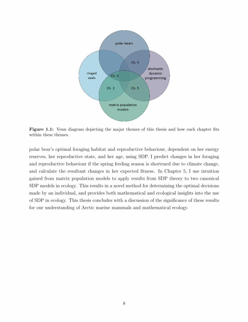
Figure 1.1: Venn diagram depicting the major themes of this thesis and how each chapter fitswithin these themes.

polar bear’s optimal foraging habitat and reproductive behaviour, dependent on her energy

reserves, her reproductive state, and her age, using SDP. I predict changes in her foraging

and reproductive behaviour if the spring feeding season is shortened due to climate change,

and calculate the resultant changes in her expected fitness. In Chapter 5, I use intuition

gained from matrix population models to apply results from SDP theory to two canonical

SDP models in ecology. This results in a novel method for determining the optimal decisions

made by an individual, and provides both mathematical and ecological insights into the use

of SDP in ecology. This thesis concludes with a discussion of the significance of these results

for our understanding of Arctic marine mammals and mathematical ecology.

8

Chapter 2

Ringed seal demography in a

changing climate

The work presented in this chapter has been published as: Reimer, J.R., Caswell, H., De-

rocher, A.E., and Lewis, M.A. (2019). Ringed seal demography in a changing climate.

Ecological Applications. doi:10.1002/eap.1855.

2.1 Introduction

With substantial climatic change predicted for the coming decades (IPCC, 2014), scientists

and managers have been tasked with anticipating and detecting resulting changes in species’

distributions and abundances. Imperative for the detection of these changes are baseline

measurements of historical populations, against which we may compare new observations.

Mathematical models can be used both to understand historical patterns and predict

future trends. Further, models may be helpful for ensuring consistency between past studies

and highlighting knowledge gaps. Looking ahead, as ecologists work to predict population

trends in novel environmental conditions, a range of modelling approaches may be helpful

(Sutherland, 2006). Approaches for assessing species’ vulnerability include standard forecast-

ing (phenomenological) models, expert opinion, trait-based approaches, and systems biology

models (Sutherland, 2006; Evans, 2012; Pacifici et al., 2015). Predictive (mechanistic) mod-

els are especially well suited for modelling populations in novel environmental conditions as

they avoid the pitfalls of extrapolating patterns outside of the range of observed conditions

(Berteaux et al., 2006; Pacifici et al., 2015). Regardless of model paradigm, models should

provide predictions against which future measurements may be compared, with assumptions

clearly stated and reevaluated as new information becomes available (Houlahan et al., 2017).

Transparent, adaptable models with testable predictions of how a population may change

9

under new environmental conditions are prerequisites for developing effective monitoring

programs as well as evidence-based wildlife management (Sutherland, 2006).

The Arctic is warming much faster than the rest of the planet (Overland et al., 2016) and

the life-history parameters of many Arctic species are correlated with changing environmental

conditions (Mech, 2000; Hunter et al., 2007; Chambellant et al., 2012; Nahrgang et al., 2014).

Changes in the sea ice regime have already been linked to changes in sea ice ecosystems

(Wassmann et al., 2011). Sea ice quality and phenology affect primary production, both

within the sea ice as well as the timing and intensity of pelagic blooms during the summer

ice free period (Arrigo, 2014; Arrigo and van Dijken, 2015). Changes in both the timing and

abundance of primary production may affect the entire food web (Bluhm and Gradinger,

2008). Furthermore, ice-associated marine mammals may depend on sea ice directly (e.g.,

as a substrate on which to give birth) or indirectly (e.g., protection from predators) (Kovacs

et al., 2011).

The responses of individuals, populations, and communities to these rapid environmental

changes will likely include complex interactions between factors. There are many unknowns,

including the speed and magnitude of environmental changes, the plasticity of species to

these new conditions, the northward range expansion of more temperate species (Kovacs

et al., 2011), and the introduction of new diseases (Burek et al., 2008). Detecting these

changes in marine mammal populations requires estimates of abundance and key life-history

parameters (e.g., survival and fertility). Unfortunately, even satisfactory baseline estimates

are unknown for many ice-associated marine mammals (Laidre et al., 2015). In light of this

uncertainty, mathematical models allow for exploration of those factors which are thought

to be important but are not yet well understood.

2.1.1 Ringed seal populations, past and future

Due to their ecology, subnivean life stages, and remote habitat, ringed seals (Pusa hisp-

ida) are one such species for whom precise abundance estimates and life-history parameters

remain elusive (Reeves, 1998; Pilfold et al., 2014b). Ringed seals are the most numerous

Arctic pinniped and have a circumpolar distribution in ice-dominated marine ecosystems

(McLaren, 1958). They are the main prey of polar bears (Ursus maritimus) (Stirling and

Archibald, 1977; Smith, 1980), a significant food source for Arctic foxes (Vulpes lagopus),

and an important species for northern communities (Smith, 1987). They are a keystone

species (Ferguson et al., 2005; Hamilton et al., 2015) and an indicator species for Arctic

environmental monitoring (Laidre et al., 2008; Chambellant and Ferguson, 2009).

Ringed seals are an ice-obligate species, dependent on the sea ice for pupping, nursing,

10

and molting (McLaren, 1958). They also depend on the presence of sufficiently deep snow

drifts in spring to dig lairs for pupping and lactation (Smith and Stirling, 1975). These life

history events and the resultant survival and reproductive rates are thus sensitive to changes

in ice phenology, ice quality, and snow depth, among multiple other factors (Smith, 1987;

Smith and Harwood, 2001; Chambellant et al., 2012; Harwood et al., 2012b).

Episodic weather events throughout the Arctic have been linked to major atmospheric

patterns operating on approximately decadal timescales (Vibe, 1967; Tremblay and Mysak,

1998; Proshutinsky et al., 2002). In the western Canadian Arctic, years of anomalously late

ice breakup occurred approximately once a decade over the past half century (Mysak, 1999;

Harwood et al., 2012b). Decadal ice cycles affecting ringed seals have also been suggested

for Hudson Bay, Canada (Ferguson et al., 2005; Chambellant et al., 2012). These events

corresponded to fluctuations in ringed seal reproduction (Smith, 1987; Stirling and Lunn,

1997; Kingsley and Byers, 1998; Harwood et al., 2012b), and body condition (Harwood et al.,

2000, 2012b; Nguyen et al., 2017). Hypothesized mechanisms include the additional energy

required to maintain breathing holes in heavier ice conditions (Harwood et al., 2012b) and

a reduction in marine productivity resulting from reduced areas of open water (i.e., reduced

leads and polynyas), and a shorter open water season (Harwood and Stirling, 1992; Stirling

and Lunn, 1997). Furthermore, seals may experience increased predation pressure from polar

bears, which use the ice as their hunting platform (Stirling et al., 1993; Stirling and Lunn,

1997). Winters with heavy ice were arguably the most significant environmental stressors

on ringed seals in the western Canadian Arctic from the 1960s through the early 2000s.

In contrast to past conditions, trends towards earlier ice breakup and a longer ice free

season have been observed in the western Canadian Arctic (Galley et al., 2008; Parkinson,

2014; Stern and Laidre, 2016) and these changes are anticipated to continue (Dumas et al.,

2006; Notz and Stroeve, 2016). As the effects of the changing climate have begun to be

documented, hypotheses have been formed as to how environmental changes may affect

ringed seal populations (Freitas et al., 2008b; Chambellant, 2010; Kelly et al., 2010). While

it may intuitively seem that reduced ice concentrations may alleviate some of the stress

experienced by ringed seals due to heavy ice in the past, benefits may be outweighed by new

stresses caused by a warmer Arctic (Stirling and Smith, 2004; Ferguson et al., 2005; Hezel

et al., 2012).

Climate change is expected to affect ringed seals in myriad ways, including effects due

to changing ecosystem productivity, food availability, and predation pressure from polar

bears (Laidre et al., 2008; Kelly et al., 2010). In addition to these projected gradual

changes, episodic events - including disease - can cause abrupt demographic changes on

shorter timescales (Ferguson et al., 2017). We do not attempt to capture all of these factors

11

here, but rather study the implications of two known mechanisms of demographic change

(Kovacs et al., 2011).

First, a decrease in seal recruitment is expected to occur with earlier ice breakup but

the mechanisms are poorly understood (Ferguson et al., 2005; Kelly et al., 2010). Ringed

seals depend on stable sea ice until they have weaned and fully transitioned to pelagic

feeding (Stirling, 2005). Premature weaning caused by the separation of pups from their

mothers is expected to negatively affect pup survival (Harwood et al., 2000; Laidre et al.,

2008). Additionally, increased thermoregulation costs may affect seal pups forced into open

water at an earlier age (Smith and Harwood, 2001), and swimming is energetically costly for

young pups (Smith et al., 1991; Lydersen and Hammill, 1993). Following unusually early ice

breakup, ringed seal pups have been documented as having significantly delayed moulting

and poor body condition (Kingsley and Byers, 1998; Smith and Harwood, 2001).

Second, reduced ringed seal recruitment has also been linked to less spring snow accu-

mulation on sea ice (Hammill and Smith, 1991; Iacozza and Ferguson, 2014). While annual

precipitation in the Arctic is expected to increase in coming decades (Hassol, 2004), the

timing and type of precipitation are expected to result in a net decrease in the accumulation

of snow on sea ice (Hezel et al., 2012). A shallower snow pack melts more quickly, and lairs

may collapse before weaning (Ferguson et al., 2005; Kelly et al., 2010). In extreme cases, the

formation of lairs may be precluded entirely (Kelly et al., 2010). Pups who do not have the

protection of a stable birth lair are more susceptible to predation by polar bears, foxes, and

avian predators (Lydersen and Smith, 1989; Hammill and Smith, 1991; Stirling and Smith,

2004). In years of shallow snow accumulation, nearly total pup mortality has been observed

(Lydersen and Smith, 1989; Hammill and Smith, 1991; Smith and Lydersen, 1991; Ferguson

et al., 2005).

Monitors in Amundsen Gulf and Prince Albert Sound, Canada, currently sample approx-

imately 100 ringed seals from the annual subsistence harvest, with the main objectives of

detecting both annual signals and longer term trends in body condition and reproduction

(Smith, 1987; Harwood et al., 2000, 2012b). The age or stage structure of harvest-based

samples are also recorded (Chambellant, 2010; Harwood et al., 2012b). Harvest samples

collected in the autumn are thought to provide the best available estimate of the structure

of the population, as all age classes are present and homogeneously distributed during the

open water period (McLaren, 1958; Smith, 1987).

12

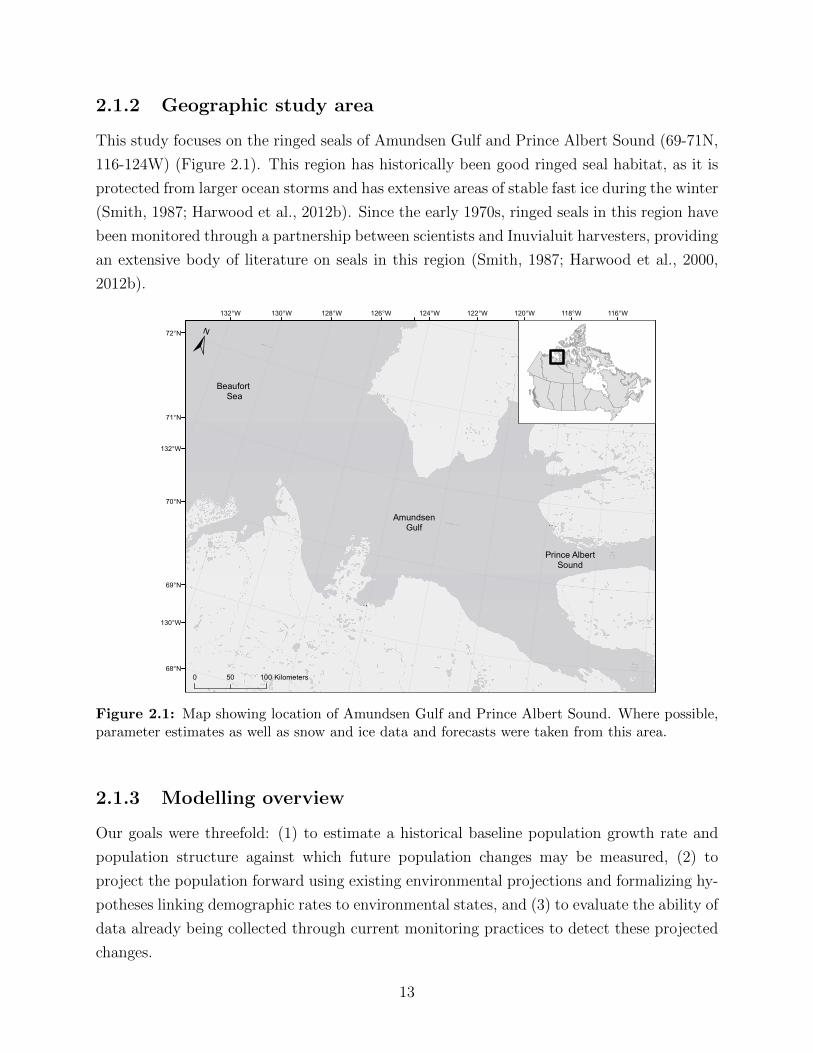
2.1.2 Geographic study area

This study focuses on the ringed seals of Amundsen Gulf and Prince Albert Sound (69-71N,

116-124W) (Figure 2.1). This region has historically been good ringed seal habitat, as it is

protected from larger ocean storms and has extensive areas of stable fast ice during the winter

(Smith, 1987; Harwood et al., 2012b). Since the early 1970s, ringed seals in this region have

been monitored through a partnership between scientists and Inuvialuit harvesters, providing

an extensive body of literature on seals in this region (Smith, 1987; Harwood et al., 2000,

2012b).

116°W118°W120°W122°W124°W126°W128°W130°W132°W

72°N

71°N

70°N

69°N

68°N

130°W

132°W

±

0 10050 Kilometers

Beaufort

Sea

Amundsen

Gulf

Prince Albert

Sound

Figure 2.1: Map showing location of Amundsen Gulf and Prince Albert Sound. Where possible,parameter estimates as well as snow and ice data and forecasts were taken from this area.

2.1.3 Modelling overview

Our goals were threefold: (1) to estimate a historical baseline population growth rate and

population structure against which future population changes may be measured, (2) to

project the population forward using existing environmental projections and formalizing hy-

potheses linking demographic rates to environmental states, and (3) to evaluate the ability of

data already being collected through current monitoring practices to detect these projected

changes.

13

We synthesized the available demographic information on ringed seals into a matrix pop-

ulation model (Section 2.2.1). Matrix population models provide a theory-rich modelling

framework with which to explore population trends (see (Caswell, 2001) for a comprehen-

sive overview). These models have been used to explore management options (Law, 1979;

Crouse et al., 1987; Rand et al., 2017) and to predict population trends under climate change

(Jenouvrier et al., 2009; Hunter et al., 2010).

We first modelled a ringed seal population under the historically observed cycles of late ice

breakup (Section 2.2.2). We did this by working through environmental models of increasing

complexity, from a constant environmental state, to a periodic environment with 10 year

cycles, to a stochastic Markovian environment (similar to the approach of Hunter et al.

(2010)). This approach provided baseline estimates of population growth and structure.

Sensitivity analyses described parameter importance, of relevance for future monitoring.

Throughout this modelling process, we uncovered gaps and inconsistencies in our knowledge

of ringed seal life-history parameters and thus suggest areas of future research.

Next, we linked demographic rates to predicted future environmental conditions by for-

malizing the hypothesized reduction in pup survival caused by earlier ice breakup and a

shallower snowpack (Section 2.2.4). We explored future population-level effects of reduced

pup survival by coupling our matrix population model to ice and snow projections for years

2017 through 2100, available through the Coupled Model Intercomparison Project Phase 5

(CMIP5) (Taylor et al., 2012).

Finally, we conducted power analyses to determine the ability of stage structured esti-

mates obtained through current sampling procedures to detect these predicted changes in

population structure from our estimated historical structure (Section 2.2.4).

2.2 Materials and methods

2.2.1 Structured population model

We first created a general demographic model for ringed seals. We considered eight distinct

stages corresponding to ages 0 (pups), 1 through 6 years (juveniles), and 7+ years (adults)

(Figure 2.2). These three stages are commonly used throughout the ringed seal literature

(Holst et al., 1999; Pilfold et al., 2012; Yurkowski et al., 2016). While the choice of age at

which a seal becomes an adult differs between studies, age 7 has been used in this region

(Pilfold et al., 2012) and corresponds to estimates of the age of first pregnancy (Harwood

et al., 2012b).

Pups are < 12 months old and experience high mortality due to predation (Stirling and

14

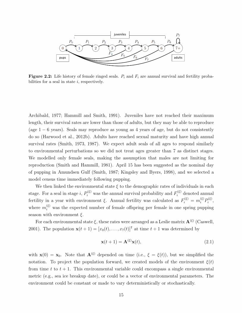
Figure 2.2: Life history of female ringed seals. Pi and Fi are annual survival and fertility proba-bilities for a seal in state i, respectively.

Archibald, 1977; Hammill and Smith, 1991). Juveniles have not reached their maximum

length, their survival rates are lower than those of adults, but they may be able to reproduce

(age 1 − 6 years). Seals may reproduce as young as 4 years of age, but do not consistently

do so (Harwood et al., 2012b). Adults have reached sexual maturity and have high annual

survival rates (Smith, 1973, 1987). We expect adult seals of all ages to respond similarly

to environmental perturbations so we did not treat ages greater than 7 as distinct stages.

We modelled only female seals, making the assumption that males are not limiting for

reproduction (Smith and Hammill, 1981). April 15 has been suggested as the nominal day

of pupping in Amundsen Gulf (Smith, 1987; Kingsley and Byers, 1998), and we selected a

model census time immediately following pupping.

We then linked the environmental state ξ to the demographic rates of individuals in each

stage. For a seal in stage i, P(ξ)i was the annual survival probability and F

(ξ)i denoted annual

fertility in a year with environment ξ. Annual fertility was calculated as F(ξ)i = m

(ξ)i P

(ξ)i ,

where m(ξ)i was the expected number of female offspring per female in one spring pupping

season with environment ξ.

For each environmental state ξ, these rates were arranged as a Leslie matrixA(ξ) (Caswell,

2001). The population x(t+ 1) = [x0(t), . . . , x7(t)]ᵀ at time t+ 1 was determined by

x(t+ 1) = A(ξ)x(t), (2.1)

with x(0) = x0. Note that A(ξ) depended on time (i.e., ξ = ξ(t)), but we simplified the

notation. To project the population forward, we created models of the environment ξ(t)

from time t to t + 1. This environmental variable could encompass a single environmental

metric (e.g., sea ice breakup date), or could be a vector of environmental parameters. The

environment could be constant or made to vary deterministically or stochastically.

15

2.2.2 Linking reproduction to historical late ice breakup

Data collected on ringed seal fertility from 1971-1981 found changes in fertility rates over

three years associated with anomalously late ice breakup (1973-1975) (Smith, 1987). We

designated 1973, 1974, and 1975 as late breakup years, denoted by ξ = l1, l2, and l3, re-

spectively. We used ξ = n to denote the remaining years with normal breakup dates. The

expected number of offspring in a given year depended on ξ(t) (Table 2.1). As survival rates

are not known to have varied over this period, we held survival rates constant for all four

environments (Table 2.1). Note that fox predation on neonate pups has here implicitly been

included in the fertility term.

stage i

demographic parameters 0 1 2 3 4 5 6 7+ source

expected m(n)i 0 0 0 0 0.098 0.144 0.195 0.406

female m(l1)i 0 0 0 0 0.085 0.125 0.169 0.352 [1]*

offspring m(l2)i 0 0 0 0 0.046 0.067 0.091 0.188

per seal m(l3)i 0 0 0 0 0.042 0.062 0.084 0.175

survival Pi 0.65 0.80 0.82 0.84 0.86 0.88 0.90 0.92 [2]‡

Table 2.1: Ringed seal annual demographic parameters and sources. Superscripts l1 through l3denote rates for three years with anomalously late ice breakup, and n denotes assumed normalconditions. [1](Smith, 1987), [2](Kelly, 1988; Kelly et al., 2010). *Fertility for stage 7+ was takento be the mean of the reported fertilities for ages 7 to 20 years, assuming the values for ages 12-20years were the same as that documented for age 11 years. ‡See Section 2.2.3 for details.

We explored the demographic effects of these late breakup events through models with

increasing environmental complexity (Hunter et al., 2010). Calculation of the population

growth rate and stable structure for each environmental model followed standard matrix

model methods (Caswell, 2001).

We first considered a constant environment characterized by its ice breakup date. We

calculated the population growth rate, log λ(ξ), by calculating the dominant eigenvalue ofA(ξ)

for each constant environment ξ ∈ {l1, l2, l3, n}. We calculated the stable stage distribution

predicted by each environmental state by calculating the right eigenvector corresponding

to the dominant eigenvalue. We calculated the elasticity (proportional sensitivity) of the

growth rate to each matrix entry.

Allowing for greater realism in the environmental model, we next considered a periodic

model, allowing for environmental fluctuations roughly analogous to those observed in the

western Canadian Arctic. We supposed that a series of years with late ice breakup, like

1973-1975, occurred once a cycle. Thus for each periodic cycle of h years, there were three

consecutive years of late breakup, l1, l2, and l3. The other h−3 years had normal ice breakup

16

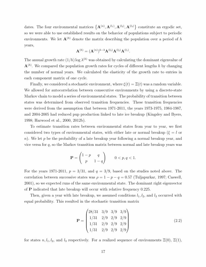
dates. The four environmental matrices{A(n),A(l1),A(l2),A(l3)

}constitute an ergodic set,

so we were able to use established results on the behavior of populations subject to periodic

environments. We let A(h) denote the matrix describing the population over a period of h

years,

A(h) = (A(n))h−3A(l3)A(l2)A(l1).

The annual growth rate (1/h) log λ(h) was obtained by calculating the dominant eigenvalue of

A(h). We compared the population growth rates for cycles of different lengths h by changing

the number of normal years. We calculated the elasticity of the growth rate to entries in

each component matrix of one cycle.

Finally, we considered a stochastic environment, where ξ(t) = Ξ(t) was a random variable.

We allowed for autocorrelation between consecutive environments by using a discrete-state

Markov chain to model a series of environmental states. The probability of transition between

states was determined from observed transition frequencies. These transition frequencies

were derived from the assumption that between 1971-2011, the years 1973-1975, 1984-1987,

and 2004-2005 had reduced pup production linked to late ice breakup (Kingsley and Byers,

1998; Harwood et al., 2000, 2012b).

To estimate transition rates between environmental states from year to year, we first

considered two types of environmental states, with either late or normal breakup (ξ = l or

n). We let p be the probability of a late breakup year following a normal breakup year, and

vice versa for q, so the Markov transition matrix between normal and late breakup years was

P =

(1− p q

p 1− q

)0 < p, q < 1.

For the years 1971-2011, p = 3/31, and q = 3/9, based on the studies noted above. The

correlation between successive states was ρ = 1− p− q = 0.57 (Tuljapurkar, 1997; Caswell,

2001), so we expected runs of the same environmental state. The dominant right eigenvector

of P indicated that late breakup will occur with relative frequency 0.225.

Then, given a year with late breakup, we assumed conditions l1, l2, and l3 occurred with

equal probability. This resulted in the stochastic transition matrix

P =

⎛⎜⎜⎜⎜⎝28/31 3/9 3/9 3/9

1/31 2/9 2/9 2/9

1/31 2/9 2/9 2/9

1/31 2/9 2/9 2/9

⎞⎟⎟⎟⎟⎠ (2.2)

for states n, l1, l2, and l3 respectively. For a realized sequence of environments Ξ(0), Ξ(1),

17

. . . , Ξ(t), we modelled the population at time t+ 1 by projecting from an initial population

vector x(0) = x0 according to x(t+ 1) = AΞ(t)AΞ(t−1) . . .AΞ(0)x0.

We calculated the stochastic growth rate, log λs, defined as the convergence of

log λs = limt→∞

1

tlog x(t).

We also simulated the population stage structure w(t) over 10000 years and recorded the

ranges of observed stage proportions. We numerically calculated the elasticity of λs to each

demographic rate in AΞ(t).

2.2.3 A note on parameter inconsistencies

For ringed seals in our study area, existing estimates of adult annual survival rates range

from 0.85 to 0.9 (Smith, 1987). When we initially set juvenile and adult survival rates

to be 0.86 (Smith, 1987) and had all remaining values the same as those we have used

for normal, high fertility years (m(n)i and P0 in Table 2.1), we obtained a negative growth

rate. Calculating the population growth rate in a constant environment following the same

methods as Section 2.2.1 yielded log λ(n) = −0.018. This implied rapid population decline

inconsistent with the known persistence of populations of ringed seals. We suspect that these

reported values are unreasonably low, given their implications for population persistence.

These reported survival values were estimated from the age structure of harvested seals,

which is a method known to often result in erroneous survival rates for long-lived animals

(Polacheck, 1985; Smith, 1987). For this reason, we chose our estimate of annual adult

survival to be P7 = 0.92. This is similar to that of other phocids with similar life expectancies

and life histories (Harkonen and Heide-Jørgensen, 1990; Harding et al., 2007; Sundqvist et al.,

2012). We assumed that the annual survival rate of juvenile seals is approximately 0.8 in

their second year and then increases incrementally until they reach adulthood (Table 2.1)

(Kelly, 1988; Kelly et al., 2010).

2.2.4 Linking pup survival to projected early ice breakup and re-

duced spring snow depth

To project the population in future conditions associated with climate change, we included

spring snow depth as an additional environmental variable, so ξ(t) was a vector of ice breakup

date and spring snow depth in year t. We assumed both early ice breakup and insufficient

snow depth contribute independently to pup survival. While predation pressure from polar

bears will likely change in the coming decades, the strength and direction of this change are

18

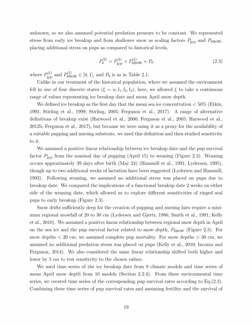
unknown, so we also assumed potential predation pressure to be constant. We represented

stress from early ice breakup and from shallower snow as scaling factors Pice and Psnow,

placing additional stress on pups as compared to historical levels,

P(ξ)0 = P

(ξ)

ice × P(ξ)snow × P0 (2.3)

where P(ξ)

ice and P(ξ)snow ∈ [0, 1], and P0 is as in Table 2.1.

Unlike in our treatment of the historical population, where we assumed the environment

fell in one of four discrete states (ξ = n, l1, l2, l3), here, we allowed ξ to take a continuous

range of values representing ice breakup date and mean April snow depth.

We defined ice breakup as the first day that the mean sea ice concentration < 50% (Etkin,

1991; Stirling et al., 1999; Stirling, 2005; Ferguson et al., 2017). A range of alternative

definitions of breakup exist (Harwood et al., 2000; Ferguson et al., 2005; Harwood et al.,

2012b; Ferguson et al., 2017), but because we were using it as a proxy for the availability of

a suitable pupping and nursing substrate, we used this definition and then studied sensitivity

to it.

We assumed a positive linear relationship between ice breakup date and the pup survival

factor Pice from the nominal day of pupping (April 15) to weaning (Figure 2.3). Weaning

occurs approximately 39 days after birth (May 24) (Hammill et al., 1991; Lydersen, 1995),

though up to two additional weeks of lactation have been suggested (Lydersen and Hammill,

1993). Following weaning, we assumed no additional stress was placed on pups due to

breakup date. We compared the implications of a functional breakup date 2 weeks on either

side of the weaning date, which allowed us to explore different sensitivities of ringed seal

pups to early breakup (Figure 2.3).

Snow drifts sufficiently deep for the creation of pupping and nursing lairs require a mini-

mum regional snowfall of 20 to 30 cm (Lydersen and Gjertz, 1986; Smith et al., 1991; Kelly

et al., 2010). We assumed a positive linear relationship between regional snow depth in April

on the sea ice and the pup survival factor related to snow depth, Psnow (Figure 2.3). For

snow depths < 20 cm, we assumed complete pup mortality. For snow depths > 30 cm, we

assumed no additional predation stress was placed on pups (Kelly et al., 2010; Iacozza and

Ferguson, 2014). We also considered the same linear relationship shifted both higher and

lower by 5 cm to test sensitivity to the chosen values.

We used time series of the ice breakup date from 9 climate models and time series of

mean April snow depth from 10 models (Section 2.2.4). From these environmental time

series, we created time series of the corresponding pup survival rates according to Eq.(2.3).

Combining these time series of pup survival rates and assuming fertility and the survival of

19

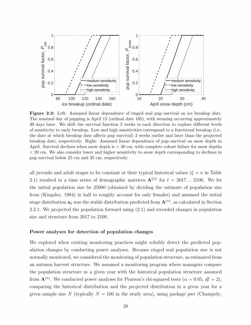
80 100 120 140 160ice breakup (ordinal date)

0

0.2

0.4

0.6

0.8

1

pup

surv

ival

fact

or,

Pic

e

medium sensitivitylow sensitivityhigh sensitivity

10 20 30 40April snow depth (cm)

0

0.2

0.4

0.6

0.8

1

pup

surv

ival

fact

or,

Psnow

medium sensitivitylow sensitivityhigh sensitivity

Figure 2.3: Left: Assumed linear dependence of ringed seal pup survival on ice breakup date.The nominal day of pupping is April 15 (ordinal date 105), with weaning occurring approximately39 days later. We shift the survival function 2 weeks in each direction to explore different levelsof sensitivity to early breakup. Low and high sensitivities correspond to a functional breakup (i.e.,the date at which breakup date affects pup survival) 2 weeks earlier and later than the projectedbreakup date, respectively. Right: Assumed linear dependence of pup survival on snow depth inApril. Survival declines when snow depth is < 30 cm, with complete cohort failure for snow depths< 20 cm. We also consider lower and higher sensitivity to snow depth corresponding to declines inpup survival below 25 cm and 35 cm, respectively.

all juvenile and adult stages to be constant at their typical historical values (ξ = n in Table

2.1) resulted in a time series of demographic matrices Aξ(t) for t = 2017 . . . 2100. We let

the initial population size be 25000 (obtained by dividing the estimate of population size

from (Kingsley, 1984) in half to roughly account for only females) and assumed the initial

stage distribution x0 was the stable distribution predicted from A(n), as calculated in Section

2.2.1. We projected the population forward using (2.1) and recorded changes in population

size and structure from 2017 to 2100.

Power analyses for detection of population changes

We explored when existing monitoring practices might reliably detect the predicted pop-

ulation changes by conducting power analyses. Because ringed seal population size is not

normally monitored, we considered the monitoring of population structure, as estimated from

an autumn harvest structure. We assumed a monitoring program where managers compare

the population structure in a given year with the historical population structure assumed

from A(n). We conducted power analyses for Pearson’s chi-squared tests (α = 0.05, df = 2),

comparing the historical distribution and the projected distribution in a given year for a

given sample size N (typically N = 100 in the study area), using package pwr (Champely,

20

2015) in R (R Core Team, 2014). Power analyses were done for each combination of snow

and ice model data, and for sample sizes ranging from N = 50 to 1000 individuals. We use

0.8 as our acceptable power value (Cohen, 1988).

Ice and snow data

Atmosphere-ocean general circulation models are the foundation of climate projections. They

inform global climate assessments such as those by the International Panel on Climate

Change (IPCC, 2014). Coordinated climate model experiments from 20 international cli-

mate modelling groups from around the world have been archived as the latest phase of

the Coupled Model Intercomparison Project (CMIP5) at the Program for Climate Model

Diagnosis and Intercomparison.

Consideration of future climate change scenarios required selection between four available

greenhouse gas scenarios. We chose projections forced with the Representative Concentration

Pathway (RCP) 8.5, colloquially known as the “business as usual” scenario. In this case,

greenhouse gas emissions continue to increase until the end of the 21st century. While this

scenario incorporates more extreme emissions than RCP 2.6, 4.5, or 6.0, we expected this to

result in the most substantial projected changes in population size and structure. This was

desirable, as we were interested in exploring our ability to detect changes, so large changes

provided an optimistic detection baseline.

We downloaded model outputs of daily sea ice concentration and monthly snow depth

on the sea ice in April from 1979—2100. Of the available models, 13 sea ice models and

14 monthly snow depth models met our baseline criteria of including a minimum of 10 grid

cells in the study area. We considered only one model output from each modelling group.

For years 1979-2005, we used outputs from historical experiments, and from 2006-2100, we

used outputs from future projections forced by RCP8.5, as defined by CMIP5 (Taylor et al.,

2012).

When possible, we retained only those models which best matched historical data. We

obtained historical data on spring ice breakup from 1979-2016 from calibrated SSMI data

from the National Snow and Ice Data Center (NSIDC), with 25 km resolution over the

entire study area. NSIDC data were processed in Arc GIS ver.10.3.1 (ESRI, Redlands, CA).

Ice concentrations were calculated from the mean of the pixel values within the defined

study area. For comparison, we calculated both the Euclidean distance and the Dynamic

Time Warping distance (a measure of distance between two numerical time series) between

observed ice breakup dates and the historical model outputs from 1979-2016 using package

TSdist (Mori et al., 2016) in R (R Core Team, 2014). The four models with the greatest

distance from observed data were consistent for both distance metrics, thus we removed

21

them and retained nine sea ice models, ∼ 70% of available models (Table A.1, Appendix

A1), which we refer to as the ice model set.

Note that in the few instances where the mean ice concentration over the study area was

not projected to fall below 50% in a given summer, we set the breakup date to be the latest

recorded for that model. A list of these instances is included in Appendix A1.

We did not have sufficient historical records with which to compare snow depth model

outputs. Instead, we took the mean values across models from 1979-2100. We then discarded

the two models with the lowest means and the two with the highest means (i.e., we kept

∼ 70% of models). We retained 10 models, which we refer to as the snow model set (Table

A.1, Appendix A1).

Unless stated otherwise, all simulations and analyses were conducted using MATLAB

2018a.

2.3 Results

2.3.1 Historical population growth and structure

The population growth rate was greatest for the model with a constant environment with

high reproductive success (ξ = n), more than double that of the periodic environment,

and nearly double that of the stochastic environment (Table 2.2). Both the periodic and

stochastic environmental models had growth rates indicative of a viable population.

The proportions of pups and juveniles in the population were lowest in constant envi-

ronments with low reproductive rates (ξ = l2, l3) (Table 2.2). The proportion of pups in

the population ranged from < 8% to nearly triple that in the stochastic environment (Table

2.2). Regardless of the environmental model, the growth rate was most sensitive to adult

survival (Figure A.3, Appendix A2).

When we considered periodic cycles of varying lengths, the population growth rate in-

creased with increasing cycle length h (Figure A.4, Appendix A2). The population growth

rate fell below 0 for cycles ≤ 6 years.

2.3.2 Projected population growth and structure

For conciseness we here use the word “simulations” to mean the population simulations done

for each combination of projections from the ice and snow model sets (90 combinations total,

see Table A.1, Appendix A1) and for each combination of the three sensitivities to ice and

snow (Figure 2.3).

In the case of low sensitivity to both decreased snow depth and earlier ice breakup, less

22

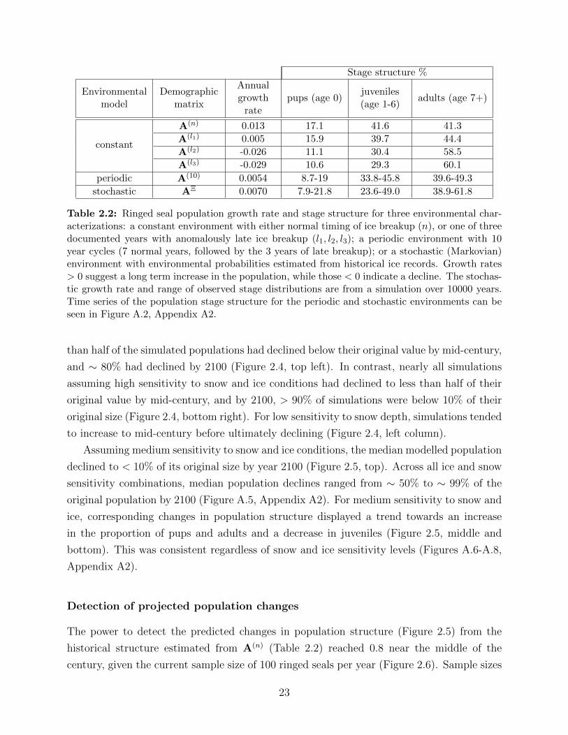
Stage structure %

Environmentalmodel

Demographicmatrix

Annualgrowthrate

pups (age 0)juveniles(age 1-6)

adults (age 7+)

constant

A(n) 0.013 17.1 41.6 41.3

A(l1) 0.005 15.9 39.7 44.4

A(l2) -0.026 11.1 30.4 58.5

A(l3) -0.029 10.6 29.3 60.1

periodic A(10) 0.0054 8.7-19 33.8-45.8 39.6-49.3

stochastic AΞ 0.0070 7.9-21.8 23.6-49.0 38.9-61.8

Table 2.2: Ringed seal population growth rate and stage structure for three environmental char-acterizations: a constant environment with either normal timing of ice breakup (n), or one of threedocumented years with anomalously late ice breakup (l1, l2, l3); a periodic environment with 10year cycles (7 normal years, followed by the 3 years of late breakup); or a stochastic (Markovian)environment with environmental probabilities estimated from historical ice records. Growth rates> 0 suggest a long term increase in the population, while those < 0 indicate a decline. The stochas-tic growth rate and range of observed stage distributions are from a simulation over 10000 years.Time series of the population stage structure for the periodic and stochastic environments can beseen in Figure A.2, Appendix A2.

than half of the simulated populations had declined below their original value by mid-century,

and ∼ 80% had declined by 2100 (Figure 2.4, top left). In contrast, nearly all simulations

assuming high sensitivity to snow and ice conditions had declined to less than half of their

original value by mid-century, and by 2100, > 90% of simulations were below 10% of their

original size (Figure 2.4, bottom right). For low sensitivity to snow depth, simulations tended

to increase to mid-century before ultimately declining (Figure 2.4, left column).

Assuming medium sensitivity to snow and ice conditions, the median modelled population

declined to < 10% of its original size by year 2100 (Figure 2.5, top). Across all ice and snow

sensitivity combinations, median population declines ranged from ∼ 50% to ∼ 99% of the

original population by 2100 (Figure A.5, Appendix A2). For medium sensitivity to snow and

ice, corresponding changes in population structure displayed a trend towards an increase

in the proportion of pups and adults and a decrease in juveniles (Figure 2.5, middle and

bottom). This was consistent regardless of snow and ice sensitivity levels (Figures A.6-A.8,

Appendix A2).

Detection of projected population changes

The power to detect the predicted changes in population structure (Figure 2.5) from the

historical structure estimated from A(n) (Table 2.2) reached 0.8 near the middle of the

century, given the current sample size of 100 ringed seals per year (Figure 2.6). Sample sizes

23

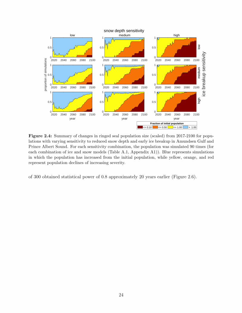
ice

brea

kup

sens

itivi

tyhi

gh

2020 2040 2060 2080 2100

year

0

0.5

1

2020 2040 2060 2080 2100

year

0

0.5

1

2020 2040 2060 2080 2100

year

0

0.5

1

med

ium

2020 2040 2060 2080 21000

0.5

1

2020 2040 2060 2080 21000

0.5

1

2020 2040 2060 2080 21000

0.5

1

prop

ortio

n of

sim

ulat

ions

high

low

2020 2040 2060 2080 21000

0.5

1medium

2020 2040 2060 2080 21000

0.5

1low

2020 2040 2060 2080 21000

0.5

1

<= 0.10 <= 0.50 <= 1.00 > 1.00

Fraction of initial population

snow depth sensitivity

Figure 2.4: Summary of changes in ringed seal population size (scaled) from 2017-2100 for popu-lations with varying sensitivity to reduced snow depth and early ice breakup in Amundsen Gulf andPrince Albert Sound. For each sensitivity combination, the population was simulated 90 times (foreach combination of ice and snow models (Table A.1, Appendix A1)). Blue represents simulationsin which the population has increased from the initial population, while yellow, orange, and redrepresent population declines of increasing severity.

of 300 obtained statistical power of 0.8 approximately 20 years earlier (Figure 2.6).

24

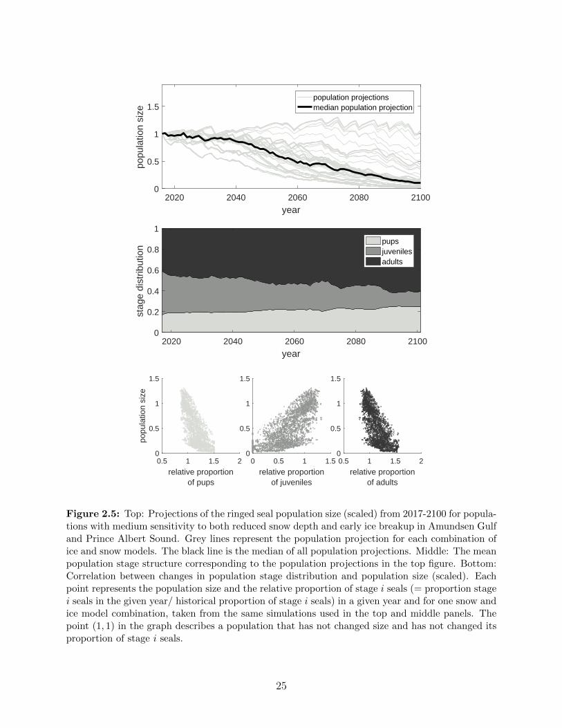
2020 2040 2060 2080 2100

year

0

0.5

1

1.5

popu

latio

n si

ze

population projectionsmedian population projection

2020 2040 2060 2080 2100

year

0

0.2

0.4

0.6

0.8

1

stag

e di

strib

utio

n

pupsjuvenilesadults

0.5 1 1.5 2

relative proportionof pups

0

0.5

1

1.5

popu

latio

n si

ze

0 0.5 1 1.5

relative proportionof juveniles

0

0.5

1

1.5

0.5 1 1.5 2

relative proportionof adults

0

0.5

1

1.5

Figure 2.5: Top: Projections of the ringed seal population size (scaled) from 2017-2100 for popula-tions with medium sensitivity to both reduced snow depth and early ice breakup in Amundsen Gulfand Prince Albert Sound. Grey lines represent the population projection for each combination ofice and snow models. The black line is the median of all population projections. Middle: The meanpopulation stage structure corresponding to the population projections in the top figure. Bottom:Correlation between changes in population stage distribution and population size (scaled). Eachpoint represents the population size and the relative proportion of stage i seals (= proportion stagei seals in the given year/ historical proportion of stage i seals) in a given year and for one snow andice model combination, taken from the same simulations used in the top and middle panels. Thepoint (1, 1) in the graph describes a population that has not changed size and has not changed itsproportion of stage i seals.

25

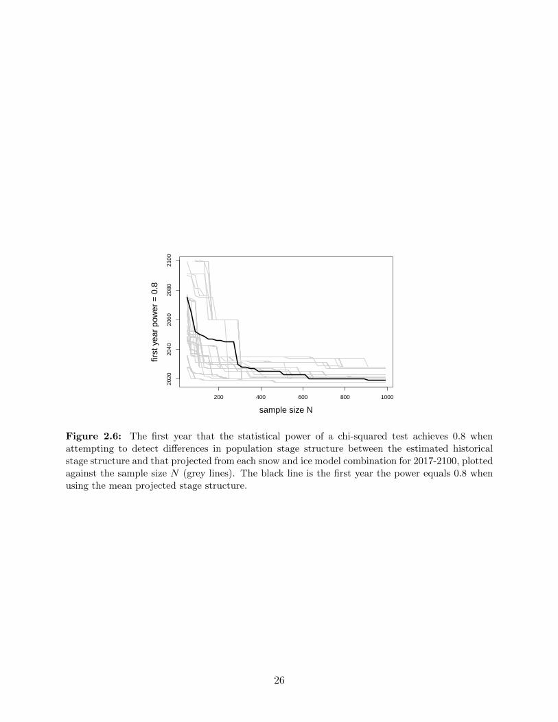
200 400 600 800 1000

2020

2040

2060

2080

2100

sample size N

first

yea

r po

wer

= 0

.8

Figure 2.6: The first year that the statistical power of a chi-squared test achieves 0.8 whenattempting to detect differences in population stage structure between the estimated historicalstage structure and that projected from each snow and ice model combination for 2017-2100, plottedagainst the sample size N (grey lines). The black line is the first year the power equals 0.8 whenusing the mean projected stage structure.

26

2.4 Discussion

2.4.1 Historical population

Through the creation of an age-structured population model, we obtained estimates of his-

torical ringed seal population growth and structure over the second half of the 20th century

and the early 21st. The higher growth rate in the stochastic environment than in the peri-

odic is unsurprising given that we created a periodic environment where late breakup years

occurred more frequently than in the stochastic environmental model (30% as compared with

22.5% of years). Given the assumptions of our model, it appears that for long-lived species

with low annual reproductive rates, periodic occurrence of weak cohorts need not lead to

population decline, as long as there is sufficient time for recovery (Figure A.4, Appendix

A2).

In the process of compiling life-history parameter estimates from previous studies, prelim-

inary results suggested that the historical population of ringed seals was in a rapid decline.

We attributed this unrealistic result to the relatively low estimates of adult survival (Sec-

tion 2.2.3). We thus selected survival rates at the upper end of what was suggested in the

literature. In spite of these optimistic parameter estimates, growth rates estimated for other

ringed seal populations are higher than our values. Baltic ringed seal annual growth was

estimated at log λ = 0.045 from aerial surveys (Sundqvist et al., 2012). This higher growth

rate may be because of the absence of predation on ringed seals from polar bears and Arctic

fox in this region (Sundqvist et al., 2012). In the eastern Canadian Arctic, ringed seal growth

was estimated at log λ = 0.0629 (Law, 1979) using values from a hypothetical, unharvested

population (McLaren, 1958). Adult survival rates were higher than those used in our study,

hypothesized to be > 0.95, contributing to the higher growth rate.

There are challenges with comparing our estimated population structures with histori-

cal harvest data from this region. During sampling in Amundsen Gulf and Prince Albert

Sound, harvest proportions were 65.6% adults, 14% juveniles, and 20.5% pups (Harwood

et al., 2012b), which most notably is a much higher percentage of adults and fewer juveniles

than our estimates. It is important, however, to note that the majority of these samples

were taken in June and July. This was before the optimal sampling period in August, when

the area is largely ice free and seals of all stages are thought to be homogeneously dis-

tributed (Smith, 1973; Holst et al., 1999). Our results support the hypothesis that sampling

during early summer may under-represent juveniles, which is consistent with hypothesized

spatial segregation of this stage in the spring (Harwood et al., 2012a; Crawford et al., 2012).

However, our estimate of ∼ 17% relative frequency of pups in the population immediately

following pupping is consistent with other estimates (mean of 20.4% in Miller et al. (1982),

27

and 16-18% in Frost (1985)).

Of the constant environments considered, higher growth rates were correlated with a

higher proportion of juveniles. This is consistent with findings from Hudson Bay, Canada,

where the population is believed to have been in decline in the 1990s and growing in the

2000s. Over these two decades, juveniles comprised 27% and 41% of the harvests in the

1990s and 2000s, respectively (Chambellant et al., 2012).

Elasticity of the population growth rate to demographic parameters indicated the im-

portance of adult survival (Figure A.3, Appendix A2), which is consistent with other long

lived mammals (Heppell et al., 2000). Unfortunately, estimates of survival past the first year

are scarce and imprecise (Smith, 1987). Changes in the survival of mature seals brought

about by changes in harvest pressure, disease, predation, or prey availability are not cur-

rently monitored through current harvest-based programs, but would have a profound effect

on population viability.

2.4.2 Projected population

We projected the ringed seal population forward by linking ringed seal pup survival to ice

and snow model forecasts. Given existing estimates for the minimal snow depth required

for lair formation and our assumed dependence of pup survival on ice breakup, our model

suggests that future reductions in mean April snow depth could be a more significant driver of

reduced pup survival than early ice breakup. In the absence of better data on the response

of pup survival to changes in snow and ice conditions, we chose the simplest justifiable

demographic responses. As more years of early breakup or reduced spring snow depth occur,

these response curves should be updated.

Changes in population structure were projected along with changes in abundance. There

is, in general, no predictable relationship between a population’s growth rate and a stable

age distribution, let alone the age distribution in a time-varying environment such as we sim-

ulated here. However, for this life history, and with the assumed effects of the environment

on the vital rates, our projections suggest a general trend in which ringed seal populations

in decline have a reduced proportion of juveniles, and an increased proportion of pups and

adults. These results were qualitatively consistent with the results from our historical popu-

lation model; populations in decline had reduced proportions of juveniles. Since determining

population size is difficult for ringed seals, population structure may conceivably be used to

detect population changes. Managers and scientists should expect to see reduced juvenile

frequency in the coming decades, and may use our model results to interpret this trend as

being suggestive of population decline, especially if it is observed in conjunction with reports

28

of reduced pup survival. While population decline cannot be concluded solely by observing

changes in population structure, the consistency (or inconsistency) of new observations with

the structure expected for a given trend may still be informative, especially if there is a

greater known context of the demographic mechanisms involved.

For the same sample size as the current monitoring program (100 seals per year), our

model predicts that the projected shift in age structure would not be reliably detected until

mid-century. Larger annual sample sizes, practical implications aside, may shorten the time

to detection. For example, increasing the sample size to 300 seals per year nearly halved the

detection time (Figure 2.6). Sampling more seals, less frequently (e.g., 300 seals every 3 years,

as compared with 100 seals every year) could also provide an alternative. However, if this

ringed seal population declines, a smaller harvest in each community is likely, complicating

any possible attempts to increase the sample size. Further, the current timing of harvest-

based sampling overlaps both the spring ice covered period as well as the late summer ice

free period. Only seals harvested in the late summer ice free period, when seals of all ages are

present, should be used to reliably assess the population age structure. Thus, the effective

sample size for these purposes is currently smaller than 100. It is also important to note that

we have used the most extreme emissions scenario, RCP 8.5, presumably resulting in the

most dramatic shifts in ringed seal population size and structure. Less extreme emissions

scenarios may result in smaller population shifts which would be more difficult to detect.

Note that the chi-squared test discussed here tests only for a difference between the historical

and projected distributions, not for the specific trend of reduced juveniles and increased pups

and adults. A more detailed statistical study treating sequential population distributions as

a time series may be able to more effectively detect specific trends.

For all of these reasons, detecting changes in population structure using the current

harvest-based monitoring program may not be feasible. Alternatively, periodic intensive

birth lair surveys (Smith and Stirling, 1975; Hammill and Smith, 1989; Kelly and Quak-

enbush, 1990) may be informative in the assessment of trends in pup production. Local

measurements of spring snow depth on the ice may also help bridge our knowledge gap

between regional snow accumulation estimates and the existence of localized drifts deep

enough for subnivean lair formation. These methods, however, would not be sufficient to

detect changes in pup recruitment due to early ice breakup.

2.4.3 Additional factors and limitations

A set of ideal conditions has been proposed for ringed seal recruitment, with ice breakup dates

that are neither too early nor too late (Chambellant et al., 2012). Breakup dates near the

29

middle of the historical range are thought to provide optimal recruitment. In light of trends

towards earlier breakup, signs of population increase may be expected in coming decades,

as late ice clearance becomes rarer, followed by a population decline as years of insufficient

snow cover and early ice breakup occur with greater frequency. Nonlinear responses such as

these to changes in sea ice complicate population projections (Gremillet et al., 2015). By

splitting this study into historical and future models and allowing for no overlap between

the two periods, we did not consider the historical implications of any years with early ice

breakup or a shallow snowpack, nor the possibility that there may still be years with late ice

breakup in the coming decades. Thus our results are, in this sense, optimistic, accounting

for only select environmental stressors at a given time.

There are limitations in our understanding of ringed seal demography and the relationship

to environmental variables. Our understanding of how demographic rates may change in

response to environmental changes currently relies on few studies covering even fewer years.

Juvenile ringed seals may emigrate to more favourable environments during years of adverse

conditions, mitigating some of the effects (Smith and Stirling, 1978; Kingsley and Byers,

1998). The age at sexual maturity and first parturition may also change in response to the

environment (Chambellant et al., 2012; Harwood et al., 2012b). Reduced body condition

of several ringed seal populations, including the Beaufort Sea, has been observed in recent

years for reasons that are poorly understood (Chambellant, 2010; Harwood et al., 2012b).

If these trends of reduced body condition continue, reduced pup production and, in extreme

cases, reduced juvenile and adult survival may occur, which we have not accounted for here.

Other factors may also play a significant role in the viability of ringed seal populations in

the coming decades. Plasticity in diet and behavior may ameliorate some effects of environ-

mental change (Laidre et al., 2008; Yurkowski et al., 2016). Range expansion by both ringed

seal predators and prey add further complexity (Laidre et al., 2008; Wassmann et al., 2011).

Other physical variables, such as ocean acidity and temperature may also affect seals and

their prey (Kelly et al., 2010). In years of early breakup, increases in primary productivity

are expected, possibly leading to greater food abundance (Sallon et al., 2011).

Changes in community structure influence and are influenced by ringed seal abundance

and distribution. In years of peak Arctic fox abundance, predation by foxes on ringed seal

pups can significantly diminish seal pup recruitment (Lydersen and Gjertz, 1986; Smith,

1987). Ringed seals are the main prey of polar bears (Stirling and Øritsland, 1995; Stirling,

2002) and a decline in ringed seals has implications on the number of polar bears that may

be sustained in an area. Changes in abundance and productivity of polar bear populations in

the eastern Beaufort Sea were correlated with declines in ringed seal production both in the

mid 1970s and 1980s (Stirling and Archibald, 1977; Stirling and Øritsland, 1995). A linear

30

relationship has been suggested between the number of polar bears and ringed seals that an

area can sustain (Stirling and Øritsland, 1995). Thus a reduction in the number of ringed

seals could cause a decrease in the polar bear population, or vice versa (Bromaghin et al.,

2015), especially in areas like the western Canadian Arctic where there are few alternative

prey species for polar bears (Thiemann et al., 2008; Cherry et al., 2011). While reductions

in spring sea ice may cause pup survival to decline, it may also negatively affect polar bear

hunting success, as polar bears rely on the sea ice to hunt in the spring. How this reduced

spring predation pressure may change our projections remains to be studied.

2.4.4 Conclusion

We have established a baseline estimate of historical population structure and growth by

synthesizing existing demographic rate estimates. This process has revealed inconsistencies

in published rates, namely adult annual survival. Given the population’s sensitivity to this

parameter, a better understanding of factors affecting adult survival is important if we are to

assess population viability as the Arctic climate changes. While we have focused our study

on Amundsen Gulf and Prince Albert Sound, the large scale atmospheric forcing leading to

past decadal cycles of ice conditions, and the general trend towards earlier ice breakup and

a shallower snow pack are shared throughout ringed seals’ range, making the results relevant

for other Arctic ringed seal populations.

Across the range of snow and ice models, and for varying sensitivity to these changing

snow and ice conditions, our projections indicate population declines in all but the most

optimistic scenarios considered, with many of these declines projecting the population to less

than half of its current size by the end of the century. This has implications for Arctic marine

ecosystems, especially for polar bears whose diets rely heavily on ringed seals. While the

current monitoring program includes other methods to assess demographic change, including

assessing reproductive rates and body condition, it is important to consider that reduced

pup survival may present a significant threat to ringed seal populations.

The chosen method of projecting a population forward and then evaluating our ability

to detect future changes using existing monitoring techniques is applicable across taxa and

environments. Even with only preliminary hypotheses of environmental effects, this exercise

can illuminate possible future scenarios and help concentrate resources towards using the

most informative monitoring methods to detect these changes. As an indicator species, ringed

seals provide information on the health of Arctic marine ecosystems, but this information

relies on our ability to detect the large scale changes resulting from climatic changes.

31

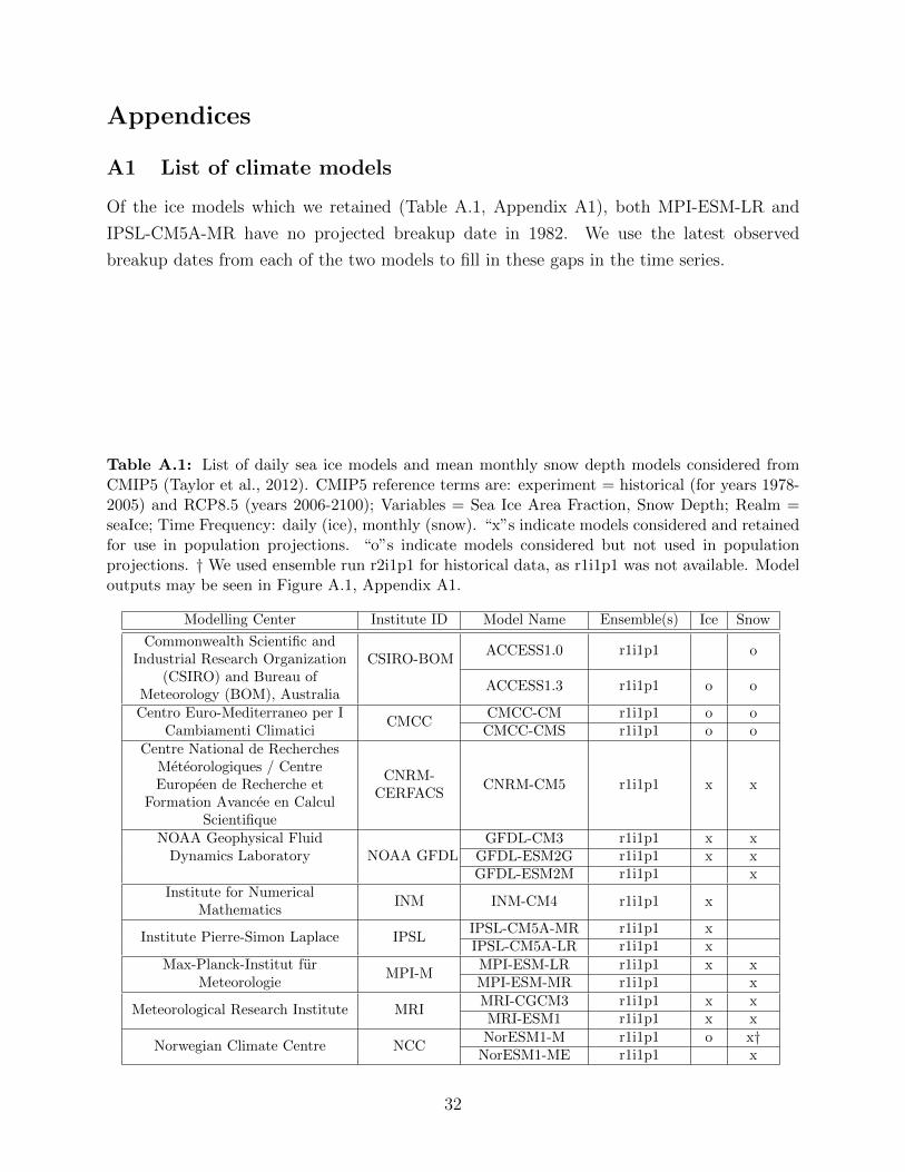
Appendices

A1 List of climate models

Of the ice models which we retained (Table A.1, Appendix A1), both MPI-ESM-LR and

IPSL-CM5A-MR have no projected breakup date in 1982. We use the latest observed

breakup dates from each of the two models to fill in these gaps in the time series.

Table A.1: List of daily sea ice models and mean monthly snow depth models considered fromCMIP5 (Taylor et al., 2012). CMIP5 reference terms are: experiment = historical (for years 1978-2005) and RCP8.5 (years 2006-2100); Variables = Sea Ice Area Fraction, Snow Depth; Realm =seaIce; Time Frequency: daily (ice), monthly (snow). “x”s indicate models considered and retainedfor use in population projections. “o”s indicate models considered but not used in populationprojections. † We used ensemble run r2i1p1 for historical data, as r1i1p1 was not available. Modeloutputs may be seen in Figure A.1, Appendix A1.

Modelling Center Institute ID Model Name Ensemble(s) Ice Snow

Commonwealth Scientific andIndustrial Research Organization CSIRO-BOM

ACCESS1.0 r1i1p1 o

(CSIRO) and Bureau ofMeteorology (BOM), Australia

ACCESS1.3 r1i1p1 o o

Centro Euro-Mediterraneo per ICMCC

CMCC-CM r1i1p1 o oCambiamenti Climatici CMCC-CMS r1i1p1 o o

Centre National de RecherchesMeteorologiques / CentreEuropeen de Recherche et

Formation Avancee en CalculScientifique

CNRM-CERFACS

CNRM-CM5 r1i1p1 x x

NOAA Geophysical FluidNOAA GFDL

GFDL-CM3 r1i1p1 x xDynamics Laboratory GFDL-ESM2G r1i1p1 x x

GFDL-ESM2M r1i1p1 xInstitute for Numerical

MathematicsINM INM-CM4 r1i1p1 x

Institute Pierre-Simon Laplace IPSLIPSL-CM5A-MR r1i1p1 xIPSL-CM5A-LR r1i1p1 x

Max-Planck-Institut furMPI-M

MPI-ESM-LR r1i1p1 x xMeteorologie MPI-ESM-MR r1i1p1 x

Meteorological Research Institute MRIMRI-CGCM3 r1i1p1 x xMRI-ESM1 r1i1p1 x x

Norwegian Climate Centre NCCNorESM1-M r1i1p1 o x†NorESM1-ME r1i1p1 x

32

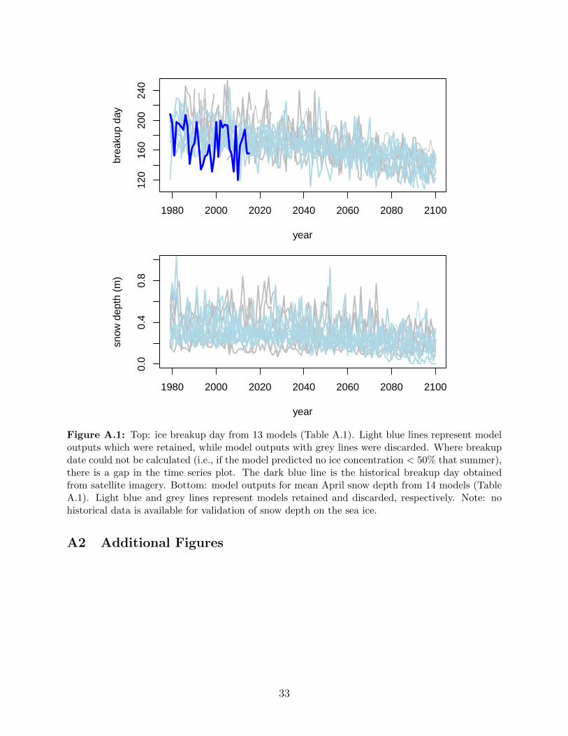
1980 2000 2020 2040 2060 2080 2100

120

160

200

240

year

brea

kup

day

1980 2000 2020 2040 2060 2080 2100

0.0

0.4

0.8

year

snow

dep

th (

m)

Figure A.1: Top: ice breakup day from 13 models (Table A.1). Light blue lines represent modeloutputs which were retained, while model outputs with grey lines were discarded. Where breakupdate could not be calculated (i.e., if the model predicted no ice concentration < 50% that summer),there is a gap in the time series plot. The dark blue line is the historical breakup day obtainedfrom satellite imagery. Bottom: model outputs for mean April snow depth from 14 models (TableA.1). Light blue and grey lines represent models retained and discarded, respectively. Note: nohistorical data is available for validation of snow depth on the sea ice.

A2 Additional Figures

33

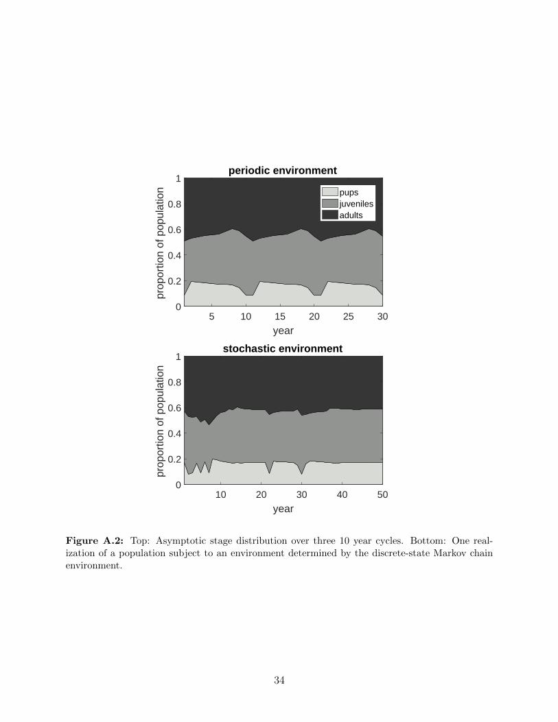
periodic environment

5 10 15 20 25 30

year

0

0.2

0.4

0.6

0.8

1

prop

ortio

n of

pop

ulat

ion pups

juvenilesadults

stochastic environment

10 20 30 40 50

year

0

0.2

0.4

0.6

0.8

1

prop

ortio

n of

pop

ulat

ion

Figure A.2: Top: Asymptotic stage distribution over three 10 year cycles. Bottom: One real-ization of a population subject to an environment determined by the discrete-state Markov chainenvironment.

34

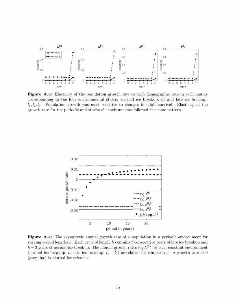
0 1 2 3 4 5 6 7+

age i

0

0.2

0.4

0.6

elas

ticity

A(n)

fertility, Fi

survival, Pi

0 1 2 3 4 5 6 7+

age i

0

0.2

0.4

0.6

elas

ticity

A(l1)

0 1 2 3 4 5 6 7+

age i

0

0.2

0.4

0.6

0.8

elas

ticity

A(l2)

0 1 2 3 4 5 6 7+

age i

0

0.2

0.4

0.6

0.8

elas

ticity

A(l3)

Figure A.3: Elasticity of the population growth rate to each demographic rate in each matrixcorresponding to the four environmental states: normal ice breakup, n; and late ice breakup,l1, l2, l3. Population growth was most sensitive to changes in adult survival. Elasticity of thegrowth rate for the periodic and stochastic environments followed the same pattern.

5 10 15 20

period (h years)

-0.03

-0.02

-0.01

0

0.01

0.02

annu

al g

row

th r

ate

log (n)

log (l1)

log (l2)

log (l3)

(1/h) log (h)

Figure A.4: The asymptotic annual growth rate of a population in a periodic environment forvarying period lengths h. Each cycle of length h contains 3 consecutive years of late ice breakup andh− 3 years of normal ice breakup. The annual growth rates log λ(ξ) for each constant environment(normal ice breakup, n; late ice breakup, l1 − l3) are shown for comparison. A growth rate of 0(grey line) is plotted for reference.

35

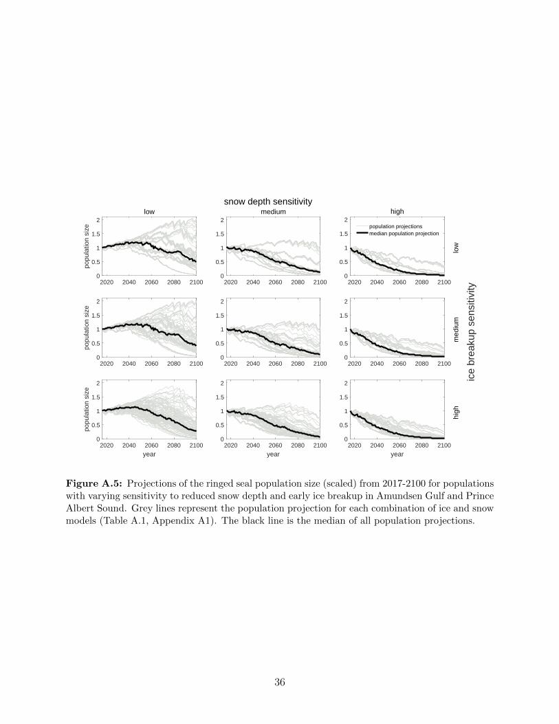
ice

brea

kup

sens

itivi

ty

2020 2040 2060 2080 2100

year

0

0.5

1

1.5

2

high

2020 2040 2060 2080 2100

year

0

0.5

1

1.5

2

2020 2040 2060 2080 2100

year

0

0.5

1

1.5

2

popu

latio

n si

ze

2020 2040 2060 2080 21000

0.5

1

1.5

2

med

ium

2020 2040 2060 2080 21000

0.5

1

1.5

2

2020 2040 2060 2080 21000

0.5

1

1.5

2

popu

latio

n si

ze

2020 2040 2060 2080 21000

0.5

1

1.5

2high

low

population projectionsmedian population projection

2020 2040 2060 2080 21000

0.5

1

1.5

2medium

2020 2040 2060 2080 21000

0.5

1

1.5

2

popu

latio

n si

ze

lowsnow depth sensitivity

Figure A.5: Projections of the ringed seal population size (scaled) from 2017-2100 for populationswith varying sensitivity to reduced snow depth and early ice breakup in Amundsen Gulf and PrinceAlbert Sound. Grey lines represent the population projection for each combination of ice and snowmodels (Table A.1, Appendix A1). The black line is the median of all population projections.

36

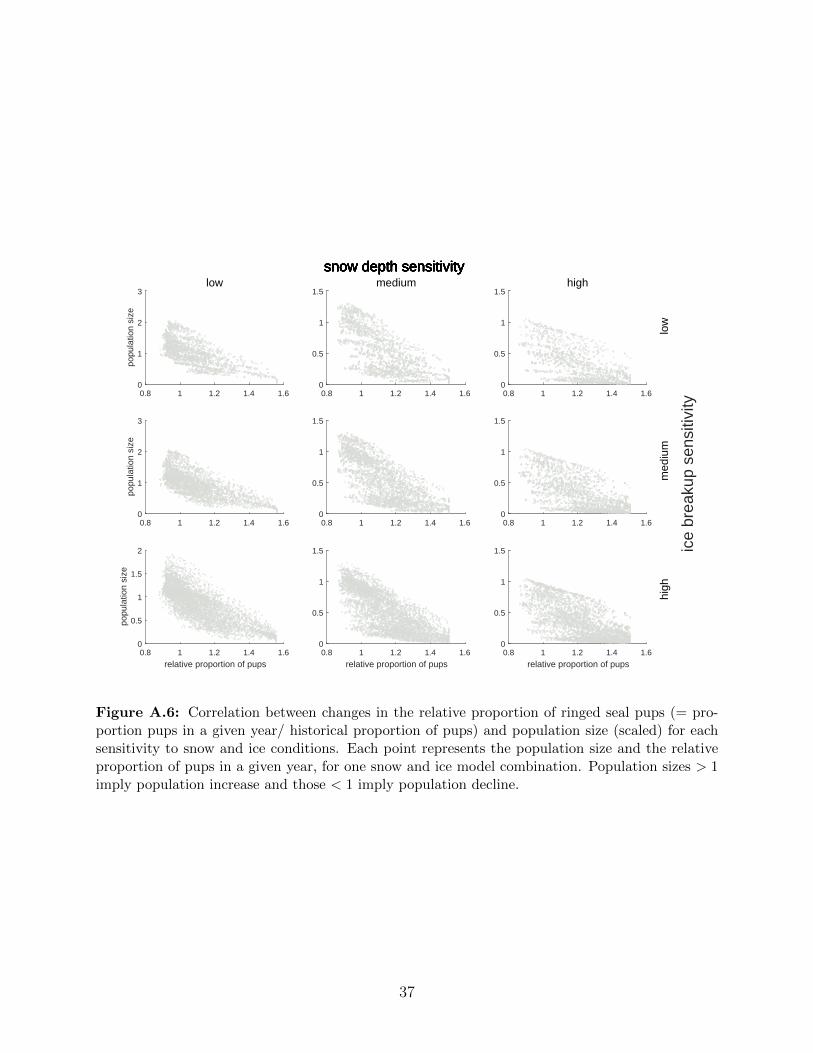
ice

brea

kup

sens

itivi

ty

0.8 1 1.2 1.4 1.6

relative proportion of pups

0

0.5

1

1.5

high

0.8 1 1.2 1.4 1.6

relative proportion of pups

0

0.5

1

1.5

2

popu

latio

n si

ze

0.8 1 1.2 1.4 1.60

0.5

1

1.5

0.8 1 1.2 1.4 1.60

0.5

1

1.5high

low

0.8 1 1.2 1.4 1.60

1

2

3

popu

latio

n si

ze

low

0.8 1 1.2 1.4 1.60

0.5

1

1.5medium

0.8 1 1.2 1.4 1.60

1

2

3

popu

latio

n si

ze

0.8 1 1.2 1.4 1.60

0.5

1

1.5

med

ium

0.8 1 1.2 1.4 1.6

relative proportion of pups

0

0.5

1

1.5

snow depth sensitivitysnow depth sensitivitysnow depth sensitivitysnow depth sensitivitysnow depth sensitivitysnow depth sensitivitysnow depth sensitivitysnow depth sensitivitysnow depth sensitivity

Figure A.6: Correlation between changes in the relative proportion of ringed seal pups (= pro-portion pups in a given year/ historical proportion of pups) and population size (scaled) for eachsensitivity to snow and ice conditions. Each point represents the population size and the relativeproportion of pups in a given year, for one snow and ice model combination. Population sizes > 1imply population increase and those < 1 imply population decline.

37

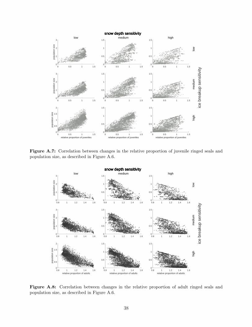
ice

brea

kup

sens

itivi

ty

0 0.5 1 1.5

relative proportion of juveniles

0

0.5

1

1.5

high

0 0.5 1 1.5

relative proportion of juveniles

0

0.5

1

1.5

2

popu

latio

n si

ze

0 0.5 1 1.50

0.5

1

1.5

0 0.5 1 1.50

0.5

1

1.5high

low

0 0.5 1 1.50

1

2

3

popu

latio

n si

ze

low

0 0.5 1 1.50

0.5

1

1.5medium

0 0.5 1 1.50

1

2

3

popu

latio

n si

ze

0 0.5 1 1.50

0.5

1

1.5

med

ium

0 0.5 1 1.5

relative proportion of juveniles

0

0.5

1

1.5

snow depth sensitivitysnow depth sensitivitysnow depth sensitivitysnow depth sensitivitysnow depth sensitivitysnow depth sensitivitysnow depth sensitivitysnow depth sensitivitysnow depth sensitivity

Figure A.7: Correlation between changes in the relative proportion of juvenile ringed seals andpopulation size, as described in Figure A.6.

ice

brea

kup

sens

itivi

ty

0.8 1 1.2 1.4 1.6

relative proportion of adults

0

0.5

1

1.5

high

0.8 1 1.2 1.4 1.6

relative proportion of adults

0

0.5

1

1.5

2

popu

latio

n si

ze

0.8 1 1.2 1.4 1.60

0.5

1

1.5

0.8 1 1.2 1.4 1.60

0.5

1

1.5high

low

0.8 1 1.2 1.4 1.60

1

2

3

popu

latio

n si

ze

low

0.8 1 1.2 1.4 1.60

0.5

1

1.5medium

0.8 1 1.2 1.4 1.60

1

2

3

popu

latio

n si

ze

0.8 1 1.2 1.4 1.60

0.5

1

1.5

med

ium

0.8 1 1.2 1.4 1.6

relative proportion of adults

0

0.5

1

1.5

snow depth sensitivitysnow depth sensitivitysnow depth sensitivitysnow depth sensitivitysnow depth sensitivitysnow depth sensitivitysnow depth sensitivitysnow depth sensitivitysnow depth sensitivity

Figure A.8: Correlation between changes in the relative proportion of adult ringed seals andpopulation size, as described in Figure A.6.

38

Chapter 3

Evidence of intraspecific prey

switching: stage-structured predation

of polar bears on ringed seals

The work presented in this chapter has been published as: Reimer, J. R., Brown, H., Beltaos-

Kerr, E., and de Vries, G. (2018) Evidence of intraspecific prey switching: stage-structured

predation of polar bears on ringed seals. Oecologia, 189(1), 133-148. doi: 10.1007/s00442-

018-4297-x.

3.1 Introduction

Prey switching is one hypothesized mechanism for stabilizing prey populations, removing

predation pressure on a depleted prey population which may allow for that population’s

recovery (Murdoch, 1969). The phenomenon may be broadly described as one in which a

predator preferentially consumes the most abundant prey species, and switches to preferen-

tially consume another if the first species becomes relatively rare (Murdoch, 1969). A variety

of mechanisms for prey switching have been proposed: the relative vulnerability of prey may

change as their frequency changes, a predator may develop a “search image” of the more

abundant prey, searching or hunting strategies between prey species may be mutually exclu-

sive, or prey species may be temporally or spatially segregated (Greenwood, 1984; Hughes

and Croy, 1993; Murdoch, 1969; Murdoch et al., 1975; Real, 1990; Tinbergen, 1960). These

mechanisms need not be restricted to interspecific effects. With slight modification of the

previous definition, we describe intraspecific prey switching as a scenario in which a predator

preferentially consumes the most abundant stage in a species, but switches to preferentially

39

consume another if that stage becomes relatively rare.

Prey species often experience variable predation during different stages in their lives. For

example, wolves (Canis lupus) prey primarily on juvenile or very old moose (Alces alces);

Walleye (Sander vitreus) prey primarily on juvenile yellow perch (Perca flavescens) (Nielsen,

1980); and sparrowhawk (Accipiter nisus L.) prey primarily on juvenile redshanks (Tringa

totanus) (Cresswell, 1994). Theoretical work on age-specific predation has revealed its com-

plexity, with models showing the inclusion of age-specific predation to be both stabilizing

and destabilizing, depending on model structure and parameter values (Hastings, 1983, 1984;

McNair, 1987; Smith and Mead, 1974). Little work has been done, however, to explore the

response by the predator if there is a sudden reduction in their preferred prey age or stage

class. In this paper, we investigate the possibility of intraspecific switching by polar bears

(Ursus maritimus) between stage classes of their primary prey species, ringed seals (Pusa

hispida), in years where environmental conditions resulted in an anomalously low number of

ringed seal pups.

Ringed seals are the most abundant Arctic pinniped, and can be found throughout the

Arctic (Reeves, 1998). Ringed seals are the primary food source of polar bears (Smith, 1980;

Stirling, 2002; Stirling and Archibald, 1977), and the population sizes of the two species are

closely linked throughout their overlapping ranges (Stirling, 2002; Stirling and Øritsland,

1995). Ringed seals rely on the sea ice as a substrate for pupping, nursing, molting, and

mating (Smith, 1987; Smith and Stirling, 1975) and each of these processes is thus sensitive to

fluctuations in ice conditions (Kelly et al., 2010). A causal relationship has been suggested

between anomalously late ice breakup in the spring and reduced ringed seal productivity

(Harwood et al., 2012b; Stirling, 2002). Hypothesized mechanisms include increased energy

required to maintain breathing holes through thicker ice, or more general reductions in

marine productivity due to reduced light (Forest et al., 2011). Decadal fluctuations in ice

breakup and corresponding reductions in ringed seal productivity have been observed in the

eastern Beaufort Sea in the mid-1960s, 1970s, 1980s, and early 2000s. Similar concurrence

of late ice breakup and reduced ringed seal productivity has been suggested in Hudson Bay,

Canada (Chambellant, 2010).

Polar bears prey heavily on ringed seal pups, so in years with low ringed seal productivity,

bears may be forced to change either the composition of their diet, reduce their energy intake,

or both. Data on seals killed by polar bears in the eastern Beaufort Sea during spring provide

some insight (Pilfold et al., 2012). In years with typical, high ringed seal productivity, one

study found that approximately 70% of observed kills were pups, while in years with late ice

breakup and reduced productivity, only 20% of observed kills were pups (Pilfold et al., 2012).

How these predation frequencies compare to the availability of each stage is unknown, which

40

leads to the questions we address here: If polar bears typically select for ringed seals pups,

how does this change in years with reduced ringed seal productivity? How does polar bear

predation during years with low ringed seal productivity impact the ringed seal population?

While these questions are simple, their answers rely on unknown information about the

stage structure and abundance of the seals available to polar bears. Estimating seal avail-

ability in this way required careful use of results from several other studies in a logical,

if somewhat technical, series of calculations. To estimate prey availability, we created a

structured population model for ringed seals. As much as possible, we parametrized our

model with values taken from the eastern Beaufort Sea. Since the early 1970s, ringed seals

in Amundsen Gulf and Prince Albert Sound have been monitored through a partnership

between scientists and Inuvialuit harvesters, providing an extensive body of literature on

seals in this area (Harwood et al., 2000, 2012b; Kingsley and Byers, 1998; Smith, 1987; Stir-

ling et al., 1977). We took estimates of both ringed seal and polar bear abundances over

both the Southern and Northern Beaufort management subpopulations, as defined by the

International Union for Conservation of Nature, Polar Bear Specialist Group (IUCN Polar

Bear Specialist Group, 2017a).

Assuming that the ratio of different types of prey in a predator’s diet is a good indicator

of the predator’s preference (Murdoch, 1969), we compared the composition of ringed seal

stages killed by polar bears (Pilfold et al., 2012) to each stage’s availability in years of both

high and low ringed seal productivity.

3.2 Methods

In years with late ice breakup, two shifts in demographic responses occur in the seal popu-

lation: (1) reduced pup production, and (2) changes in survival probabilities resulting from

shifts in predation pressure by polar bears. The reduction in pup production between high

and low productivity years has been documented (Smith, 1987), and several estimates of

survival probabilities exist for typical years with high productivity (Table 3.1). In low pro-

ductivity years, however, changes in predation pressure and implications for annual survival

probabilities are unknown. We estimated the age-specific predation pressure and survival

probabilities in low productivity years by combining existing empirical studies with results

from matrix model theory. Once survival probabilities incorporating predation pressure were

obtained for years of both high and low productivity, we could then explore population level

effects of age-specific predation.

The set-up of our study is illustrated in Figure 3.1. Methods are described in the order in

which they had to be carried out (i.e., working downwards through Figure 3.1), so that all of

41

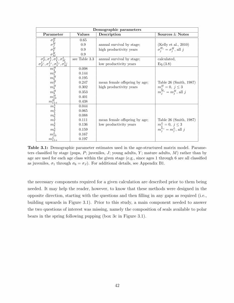
Demographic parametersParameter Values Description Sources & Notes

σHP 0.65

σHJ 0.9 annual survival by stage; (Kelly et al., 2010)

σHY 0.9 high productivity years σHc

j = σHj , all j

σHM 0.9

σLP , σ

LJ , σ

LY , σ

LM see Table 3.3 annual survival by stage; calculated,

σLc

P , σLc

J , σLc

Y , σLc

M low productivity years Eq.(3.8)mH

4 0.098mH

5 0.144mH

6 0.195mH

7 0.247 mean female offspring by age; Table 26 (Smith, 1987)mH

8 0.302 high productivity years mHj = 0, j ≤ 3

mH9 0.353 mHc

j = mHj , all j

mH10 0.401

mH11+ 0.438mL

4 0.044mL

5 0.065mL

6 0.088mL

7 0.111 mean female offspring by age; Table 26 (Smith, 1987)mL

8 0.136 low productivity years mLj = 0, j ≤ 3

mL9 0.159 mLc

j = mLj , all j

mL10 0.167

mL11+ 0.197

Table 3.1: Demographic parameter estimates used in the age-structured matrix model. Parame-ters classified by stage (pups, P ; juveniles, J ; young adults, Y ; mature adults, M) rather than byage are used for each age class within the given stage (e.g., since ages 1 through 6 are all classifiedas juveniles, σ1 through σ6 = σJ). For additional details, see Appendix B1.

the necessary components required for a given calculation are described prior to them being

needed. It may help the reader, however, to know that these methods were designed in the

opposite direction, starting with the questions and then filling in any gaps as required (i.e.,

building upwards in Figure 3.1). Prior to this study, a main component needed to answer

the two questions of interest was missing, namely the composition of seals available to polar

bears in the spring following pupping (box 3c in Figure 3.1).

42

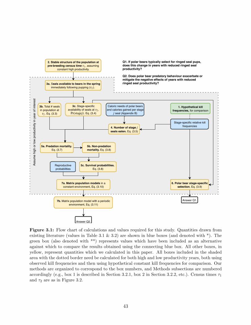
2. Stable structure of the population atpre-breeding census time , assuming

constant high productivity.τ1

3a. Seals available to bears in the springimmediately following pupping ( ). τ2

4. Number of stage seals eaten. Eq. (3.5)

j

Caloric needs of polar bearsand calories gained per stage

seal (Appendix B)j

7a. Matrix population models in aconstant environment, Eq. (3.10)

Stage-specific relative killfrequencies

1. Hypothetical killfrequencies, for comparison

Answer Q2.

Answer Q1.7b. Matrix population model with a periodicenvironment, Eq. (3.11)

6. Polar bear stage-specificselection, Eq. (3.9)

Assu

me

high

or l

ow p

rodu

ctiv

ity in

yea

r of i

nter

est

5b. Non-predationmortality. Eq. (3.8)

5a. Predation mortality. Eq. (3.7)

Q1. If polar bears typically select for ringed seal pups,does this change in years with reduced ringed sealproductivity? Q2. Does polar bear predatory behaviour exacerbate ormitigate the negative effects of years with reducedringed seal productivity?

Reproductiveprobabilities

5c. Survival probabilities. Eq. (3.8)

3b. Total # sealsin population at

. Eq. (3.3)τ2

3c. Stage-specificavailability of seals at ,

. Eq. (3.4)τ2

Pr(stagej)

Figure 3.1: Flow chart of calculations and values required for this study. Quantities drawn fromexisting literature (values in Table 3.1 & 3.2) are shown in blue boxes (and denoted with *). Thegreen box (also denoted with **) represents values which have been included as an alternativeagainst which to compare the results obtained using the connecting blue box. All other boxes, inyellow, represent quantities which we calculated in this paper. All boxes included in the shadedarea with the dotted border need be calculated for both high and low productivity years, both usingobserved kill frequencies and then using hypothetical constant kill frequencies for comparison. Ourmethods are organized to correspond to the box numbers, and Methods subsections are numberedaccordingly (e.g., box 1 is described in Section 3.2.1, box 2 in Section 3.2.2, etc.). Census times τ1and τ2 are as in Figure 3.2.

43

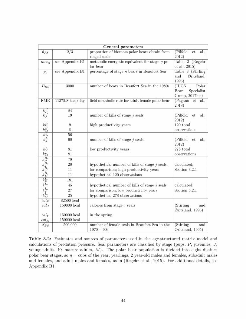
General parametersθRS 2/3 proportion of biomass polar bears obtain from

ringed seals(Pilfold et al.,2012)

meeη see Appendix B1 metabolic energetic equivalent for stage η po-lar bear

Table 2 (Regehret al., 2015)

pη see Appendix B1 percentage of stage η bears in Beaufort Sea Table 3 (Stirlingand Øritsland,1995)

BBS 3000 number of bears in Beaufort Sea in the 1980s (IUCN PolarBear SpecialistGroup, 2017b,c)

FMR 11375.8 kcal/day field metabolic rate for adult female polar bear (Pagano et al.,2018)

kHP 84kHJ 19 number of kills of stage j seals; (Pilfold et al.,

2012)kHY 9 high productivity years 120 totalkHM 8 observationskLP 56kLJ 60 number of kills of stage j seals; (Pilfold et al.,

2012)kLY 81 low productivity years 278 totalkLM 81 observations

kHc

P 78

kHc

J 20 hypothetical number of kills of stage j seals, calculated;

kHc

Y 11 for comparison; high productivity years Section 3.2.1

kHc

M 11 hypothetical 120 observations

kLc

P 181

kLc

J 45 hypothetical number of kills of stage j seals, calculated;

kLc

Y 27 for comparison; low productivity years Section 3.2.1

kLc

M 25 hypothetical 278 observationscalP 82500 kcalcalJ 150000 kcal calories from stage j seals (Stirling and

Øritsland, 1995)calY 150000 kcal in the springcalM 150000 kcalSBS 500,000 number of female seals in Beaufort Sea in the

1970− 90s(Stirling andØritsland, 1995)

Table 3.2: Estimates and sources of parameters used in the age-structured matrix model andcalculations of predation pressure. Seal parameters are classified by stage (pups, P ; juveniles, J ;young adults, Y ; mature adults, M). The polar bear population is divided into eight distinctpolar bear stages, so η = cubs of the year, yearlings, 2 year-old males and females, subadult malesand females, and adult males and females, as in (Regehr et al., 2015). For additional details, seeAppendix B1.

44

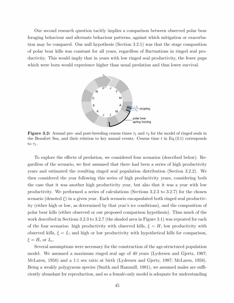
Our second research question tacitly implies a comparison between observed polar bear

foraging behaviour and alternate behaviour patterns, against which mitigation or exacerba-

tion may be compared. Our null hypothesis (Section 3.2.1) was that the stage composition

of polar bear kills was constant for all years, regardless of fluctuations in ringed seal pro-

ductivity. This would imply that in years with low ringed seal productivity, the fewer pups

which were born would experience higher than usual predation and thus lower survival.

Figure 3.2: Annual pre- and post-breeding census times τ1 and τ2 for the model of ringed seals inthe Beaufort Sea, and their relation to key annual events. Census time t in Eq.(3.1) correspondsto τ1.

To explore the effects of predation, we considered four scenarios (described below). Re-

gardless of the scenario, we first assumed that there had been a series of high productivity

years and estimated the resulting ringed seal population distribution (Section 3.2.2). We

then considered the year following this series of high productivity years, considering both

the case that it was another high productivity year, but also that it was a year with low

productivity. We performed a series of calculations (Sections 3.2.3 to 3.2.7) for the chosen

scenario (denoted ξ) in a given year. Each scenario encapsulated both ringed seal productiv-

ity (either high or low, as determined by that year’s ice conditions), and the composition of

polar bear kills (either observed or our proposed comparison hypothesis). Thus much of the

work described in Sections 3.2.3 to 3.2.7 (the shaded area in Figure 3.1) was repeated for each

of the four scenarios: high productivity with observed kills, ξ = H; low productivity with

observed kills, ξ = L; and high or low productivity with hypothetical kills for comparison,

ξ = Hc or Lc.

Several assumptions were necessary for the construction of the age-structured population

model. We assumed a maximum ringed seal age of 40 years (Lydersen and Gjertz, 1987;

McLaren, 1958) and a 1:1 sex ratio at birth (Lydersen and Gjertz, 1987; McLaren, 1958).

Being a weakly polygynous species (Smith and Hammill, 1981), we assumed males are suffi-

ciently abundant for reproduction, and so a female-only model is adequate for understanding

45

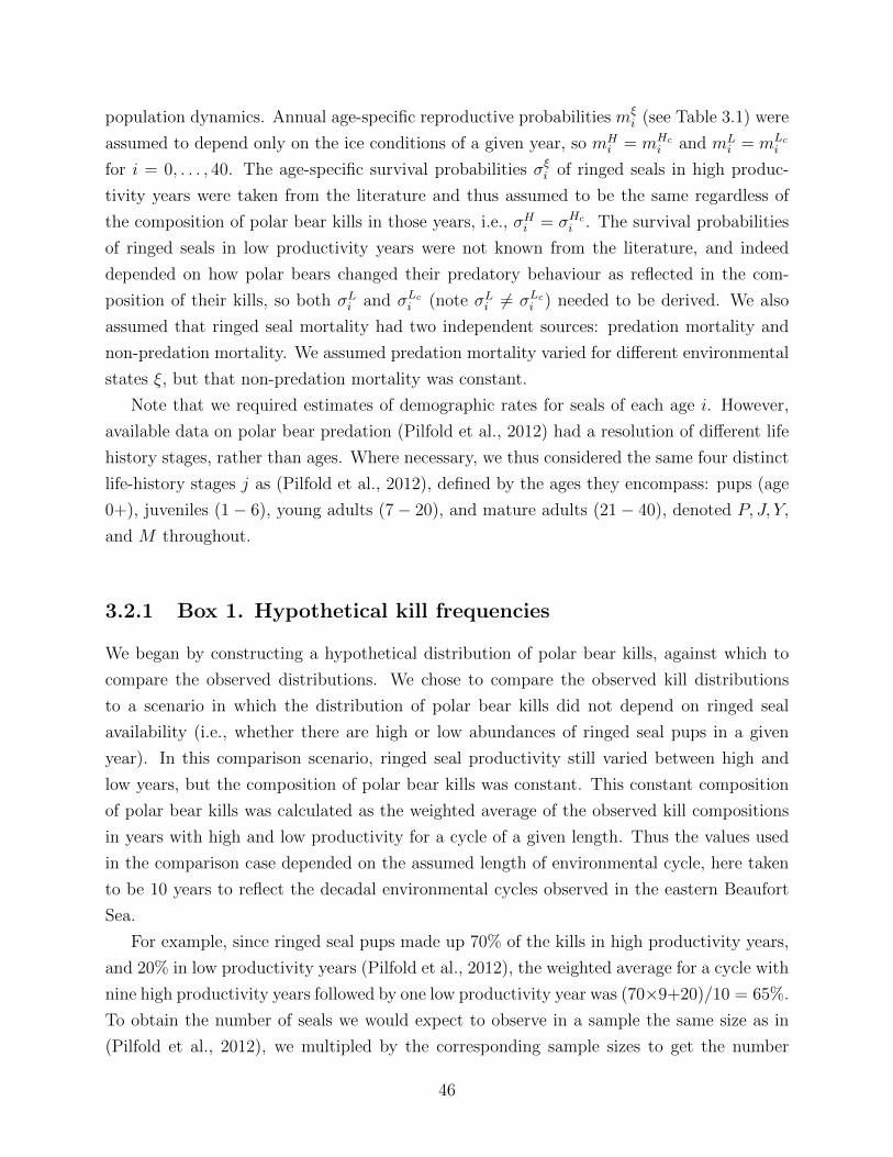
population dynamics. Annual age-specific reproductive probabilities mξi (see Table 3.1) were

assumed to depend only on the ice conditions of a given year, so mHi = mHc

i and mLi = mLc

i

for i = 0, . . . , 40. The age-specific survival probabilities σξi of ringed seals in high produc-

tivity years were taken from the literature and thus assumed to be the same regardless of

the composition of polar bear kills in those years, i.e., σHi = σHc

i . The survival probabilities

of ringed seals in low productivity years were not known from the literature, and indeed

depended on how polar bears changed their predatory behaviour as reflected in the com-

position of their kills, so both σLi and σLc

i (note σLi = σLc

i ) needed to be derived. We also

assumed that ringed seal mortality had two independent sources: predation mortality and

non-predation mortality. We assumed predation mortality varied for different environmental

states ξ, but that non-predation mortality was constant.

Note that we required estimates of demographic rates for seals of each age i. However,

available data on polar bear predation (Pilfold et al., 2012) had a resolution of different life

history stages, rather than ages. Where necessary, we thus considered the same four distinct

life-history stages j as (Pilfold et al., 2012), defined by the ages they encompass: pups (age

0+), juveniles (1− 6), young adults (7− 20), and mature adults (21− 40), denoted P, J, Y,

and M throughout.

3.2.1 Box 1. Hypothetical kill frequencies

We began by constructing a hypothetical distribution of polar bear kills, against which to

compare the observed distributions. We chose to compare the observed kill distributions

to a scenario in which the distribution of polar bear kills did not depend on ringed seal

availability (i.e., whether there are high or low abundances of ringed seal pups in a given

year). In this comparison scenario, ringed seal productivity still varied between high and

low years, but the composition of polar bear kills was constant. This constant composition

of polar bear kills was calculated as the weighted average of the observed kill compositions

in years with high and low productivity for a cycle of a given length. Thus the values used

in the comparison case depended on the assumed length of environmental cycle, here taken

to be 10 years to reflect the decadal environmental cycles observed in the eastern Beaufort

Sea.

For example, since ringed seal pups made up 70% of the kills in high productivity years,

and 20% in low productivity years (Pilfold et al., 2012), the weighted average for a cycle with

nine high productivity years followed by one low productivity year was (70×9+20)/10 = 65%.

To obtain the number of seals we would expect to observe in a sample the same size as in

(Pilfold et al., 2012), we multipled by the corresponding sample sizes to get the number

46

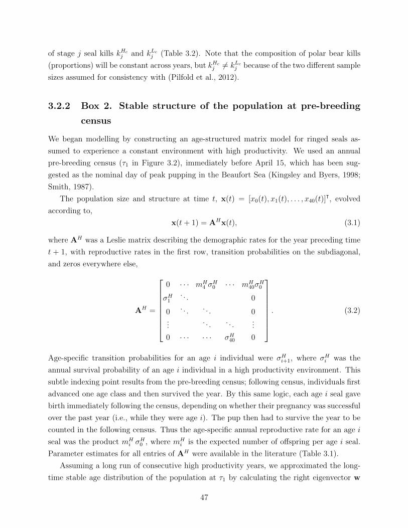
of stage j seal kills kHcj and kLc

j (Table 3.2). Note that the composition of polar bear kills

(proportions) will be constant across years, but kHcj = kLc

j because of the two different sample

sizes assumed for consistency with (Pilfold et al., 2012).

3.2.2 Box 2. Stable structure of the population at pre-breeding

census

We began modelling by constructing an age-structured matrix model for ringed seals as-

sumed to experience a constant environment with high productivity. We used an annual

pre-breeding census (τ1 in Figure 3.2), immediately before April 15, which has been sug-

gested as the nominal day of peak pupping in the Beaufort Sea (Kingsley and Byers, 1998;

Smith, 1987).

The population size and structure at time t, x(t) = [x0(t), x1(t), . . . , x40(t)]ᵀ, evolved

according to,

x(t+ 1) = AHx(t), (3.1)

where AH was a Leslie matrix describing the demographic rates for the year preceding time

t + 1, with reproductive rates in the first row, transition probabilities on the subdiagonal,

and zeros everywhere else,

AH =

⎡⎢⎢⎢⎢⎢⎢⎢⎣

0 · · · mH4 σ

H0 · · · mH

40σH0

σH1

. . . 0

0. . . . . . 0

.... . . . . .

...

0 · · · · · · σH40 0

⎤⎥⎥⎥⎥⎥⎥⎥⎦. (3.2)

Age-specific transition probabilities for an age i individual were σHi+1, where σ

Hi was the

annual survival probability of an age i individual in a high productivity environment. This

subtle indexing point results from the pre-breeding census; following census, individuals first

advanced one age class and then survived the year. By this same logic, each age i seal gave

birth immediately following the census, depending on whether their pregnancy was successful

over the past year (i.e., while they were age i). The pup then had to survive the year to be

counted in the following census. Thus the age-specific annual reproductive rate for an age i

seal was the product mHi σ

H0 , where mH

i is the expected number of offspring per age i seal.

Parameter estimates for all entries of AH were available in the literature (Table 3.1).

Assuming a long run of consecutive high productivity years, we approximated the long-

time stable age distribution of the population at τ1 by calculating the right eigenvector w

47

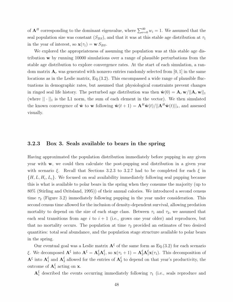
of AH corresponding to the dominant eigenvalue, where∑40

ν=0wi = 1. We assumed that the

seal population size was constant (SBS), and that it was at this stable age distribution at τ1

in the year of interest, so x(τ1) = w SBS.

We explored the appropriateness of assuming the population was at this stable age dis-

tribution w by running 10000 simulations over a range of plausible perturbations from the

stable age distribution to explore convergence rates. At the start of each simulation, a ran-

dom matrix Ar was generated with nonzero entries randomly selected from [0, 1] in the same

locations as in the Leslie matrix, Eq.(3.2). This encompassed a wide range of plausible fluc-

tuations in demographic rates, but assumed that physiological constraints prevent changes

in ringed seal life history. The perturbed age distribution was then w(0) = Ar w/||Ar w||1(where || · ||1 is the L1 norm, the sum of each element in the vector). We then simulated

the known convergence of w to w following w(t + 1) = AHw(t)/||AHw(t)||1, and assessed

visually.

3.2.3 Box 3. Seals available to bears in the spring

Having approximated the population distribution immediately before pupping in any given

year with w, we could then calculate the post-pupping seal distribution in a given year

with scenario ξ. Recall that Sections 3.2.3 to 3.2.7 had to be completed for each ξ in

{H,L,Hc, Lc}. We focused on seal availability immediately following seal pupping because

this is what is available to polar bears in the spring when they consume the majority (up to

80% (Stirling and Øritsland, 1995)) of their annual calories. We introduced a second census

time τ2 (Figure 3.2) immediately following pupping in the year under consideration. This

second census time allowed for the inclusion of density-dependent survival, allowing predation

mortality to depend on the size of each stage class. Between τ1 and τ2, we assumed that

each seal transitions from age i to i + 1 (i.e., grows one year older) and reproduces, but

that no mortality occurs. The population at time τ2 provided an estimates of two desired

quantities: total seal abundance, and the population stage structure available to polar bears

in the spring.

Our eventual goal was a Leslie matrix Aξ of the same form as Eq.(3.2) for each scenario

ξ. We decomposed Aξ into Aξ = Aξ2A

ξ1, so x(τ1 + 1) = Aξ

2Aξ1x(τ1). This decomposition of

Aξ into Aξ1 and Aξ

2 allowed for the entries of Aξ2 to depend on that year’s productivity, the

outcome of Aξ1 acting on x.

Aξ1 described the events occurring immediately following τ1 (i.e., seals reproduce and

48

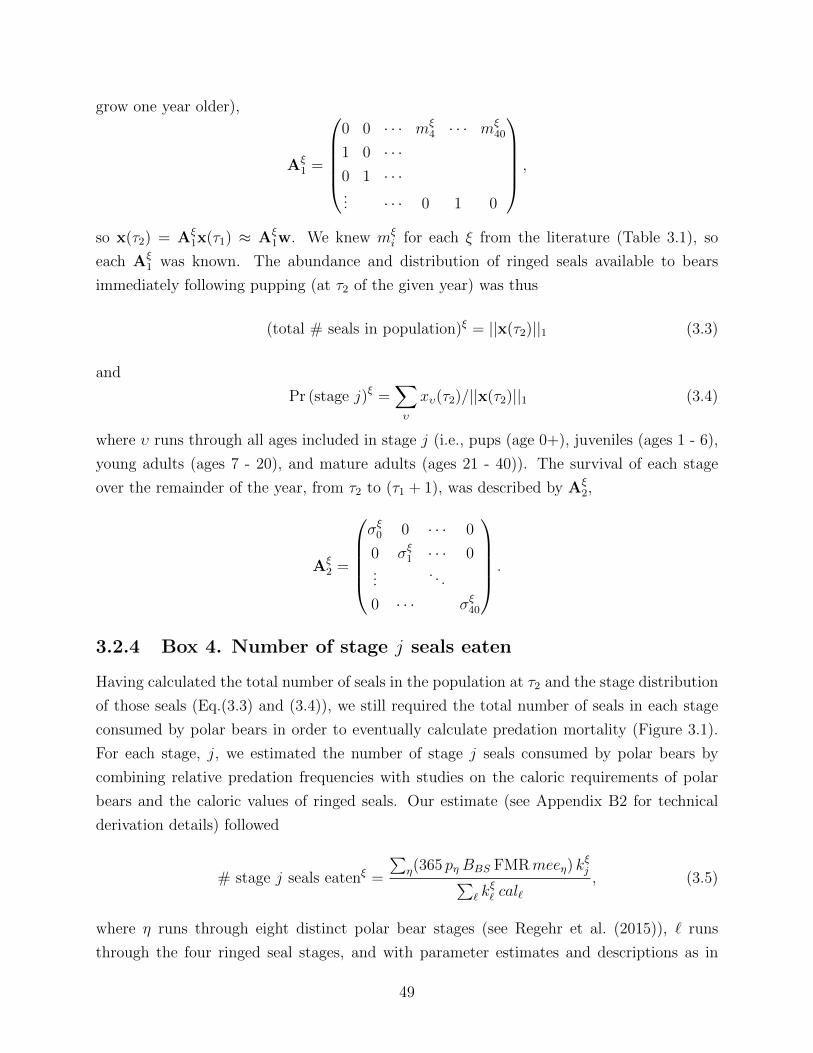
grow one year older),

Aξ1 =

⎛⎜⎜⎜⎜⎝0 0 · · · mξ

4 · · · mξ40

1 0 · · ·0 1 · · ·... · · · 0 1 0

⎞⎟⎟⎟⎟⎠ ,

so x(τ2) = Aξ1x(τ1) ≈ Aξ

1w. We knew mξi for each ξ from the literature (Table 3.1), so

each Aξ1 was known. The abundance and distribution of ringed seals available to bears

immediately following pupping (at τ2 of the given year) was thus

(total # seals in population)ξ = ||x(τ2)||1 (3.3)

and

Pr (stage j)ξ =∑υ

xυ(τ2)/||x(τ2)||1 (3.4)

where υ runs through all ages included in stage j (i.e., pups (age 0+), juveniles (ages 1 - 6),

young adults (ages 7 - 20), and mature adults (ages 21 - 40)). The survival of each stage

over the remainder of the year, from τ2 to (τ1 + 1), was described by Aξ2,

Aξ2 =

⎛⎜⎜⎜⎜⎝σξ0 0 · · · 0

0 σξ1 · · · 0

.... . .

0 · · · σξ40

⎞⎟⎟⎟⎟⎠ .

3.2.4 Box 4. Number of stage j seals eaten

Having calculated the total number of seals in the population at τ2 and the stage distribution

of those seals (Eq.(3.3) and (3.4)), we still required the total number of seals in each stage

consumed by polar bears in order to eventually calculate predation mortality (Figure 3.1).

For each stage, j, we estimated the number of stage j seals consumed by polar bears by

combining relative predation frequencies with studies on the caloric requirements of polar

bears and the caloric values of ringed seals. Our estimate (see Appendix B2 for technical

derivation details) followed

# stage j seals eatenξ =

∑η(365 pη BBS FMRmeeη) k

ξj∑

ℓ kξℓ calℓ

, (3.5)

where η runs through eight distinct polar bear stages (see Regehr et al. (2015)), ℓ runs

through the four ringed seal stages, and with parameter estimates and descriptions as in

49

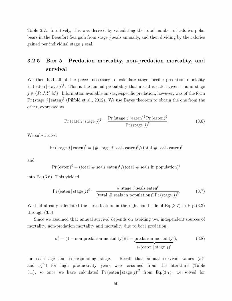
Table 3.2. Intuitively, this was derived by calculating the total number of calories polar

bears in the Beaufort Sea gain from stage j seals annually, and then dividing by the calories

gained per individual stage j seal.

3.2.5 Box 5. Predation mortality, non-predation mortality, and

survival

We then had all of the pieces necessary to calculate stage-specific predation mortality

Pr (eaten | stage j)ξ. This is the annual probability that a seal is eaten given it is in stage

j ∈ {P, J, Y,M}. Information available on stage-specific predation, however, was of the form

Pr (stage j | eaten)ξ (Pilfold et al., 2012). We use Bayes theorem to obtain the one from the

other, expressed as

Pr (eaten | stage j)ξ = Pr (stage j | eaten)ξ Pr (eaten)ξ

Pr (stage j)ξ. (3.6)

We substituted

Pr (stage j | eaten)ξ = (# stage j seals eaten)ξ/(total # seals eaten)ξ

and

Pr (eaten)ξ = (total # seals eaten)ξ/(total # seals in population)ξ

into Eq.(3.6). This yielded

Pr (eaten | stage j)ξ = # stage j seals eatenξ

(total # seals in population)ξ Pr (stage j)ξ. (3.7)

We had already calculated the three factors on the right-hand side of Eq.(3.7) in Eqs.(3.3)

through (3.5).

Since we assumed that annual survival depends on avoiding two independent sources of

mortality, non-predation mortality and mortality due to bear predation,

σξi = (1− non-predation mortalityξi )(1− predation mortalityξi⏞ ⏟⏟ ⏞

Pr(eaten | stage j)ξ), (3.8)

for each age and corresponding stage. Recall that annual survival values (σHi

and σHci ) for high productivity years were assumed from the literature (Table

3.1), so once we have calculated Pr (eaten | stage j)H from Eq.(3.7), we solved for

50

(non-predation mortalityHi ). Because we assumed that non-predation mortality does

not depend on the timing of ice breakup and is approximately constant across years,

then (non-predation mortalityξi ) = (non-predation mortalityHi ) for ξ = Hc, L, Lc. Using

Pr (eaten | stage j)L and Pr (eaten | stage j)Lc as calculated from Eq.(3.7), we then obtained

σLi and σLc

i , which included both the effects of reduced ringed seal productivity as well as

resultant changes in predation mortality.

3.2.6 Box 6. Polar bear stage-specific selection

Sections 3.2.1-3.2.3 included all of the components required to address the first of our two

main questions, that of polar bear predation preference in high versus low productivity years

(Q1 in Figure 3.1). We defined selection on each stage j for each scenario ξ as

selectionξj =

proportion predated

proportion available=

(kξj/∑

ℓ kξℓ )

Pr (stage j)ξ(3.9)

where ℓ runs through the four ringed seal stages, and Pr (stage j)ξ is as in Eq.(3.4). If

selectionξj < 1, this may be interpreted as polar bears preying on proportionally fewer stage

j individuals than what are available. If selectionξj = 1, this suggests polar bears are preying

on stage j seals with the same frequency with which seals in stage j occur in the population.

If selectionξj > 1, polar bears are predating more on stage j seals than their relative frequency

in the population.

3.2.7 Box 7. Matrix population models

Using the results from Sections 3.2.1-3.2.5, we addressed our second question (Q2 in Figure

3.1). All parameters σξi and mξ

i for each scenario ξ had been estimated either from the

literature or through our calculations. Thus we formed four Leslie matrices AH ,AL,AHc

and ALc , each of the form (3.2) but with entries corresponding to ξ. Recall that σHi = σHc

i

and mHi = mHc

i , so AH = AHc .

If we assumed a constant environment ξ, the population evolved according to

x(t+ 1) = Aξx(t), ξ = H,L,Hc, Lc. (3.10)

To determine the impact of the decadal cycles suggested to occur in the Beaufort Sea with a

periodic matrix model, we assumed a periodic environment over 10 years, characterized by

nine years with high productivity, followed by one year with low productivity. One cycle for

51

the scenario with observed polar bear kill proportions was described by B = AL(AH)9, so

x(t+ 10) = Bx(t). (3.11)

Similarly, for the case with the hypothetical comparison kill proportions, Bc = ALc(AHc

)9.

We calculated the long-term growth rate and age distribution of a population subject

to each constant environment, AH , AL, and ALc , as well as the periodic environments

B and Bc by calculating the matrices’ dominant eigenvalues (λ) and corresponding right

eigenvectors (see (Caswell, 2001) for a good overview). A negative population growth rate

(i.e., log λ < 0) implies population decline, and log λ > 0 implies long-term exponential

population growth. We addressed our second question through the analysis and comparison

of these matrix models between the scenario with observed kill frequencies and the scenario

with the hypothetical frequencies (Figure 3.1).

3.2.8 Sensitivity to model parameters

This work relied on model parameters taken from the relevant literature, which introduced

several sources of uncertainty into the results. To better understand this, we performed both

qualitative and quantitative sensitivity analyses where appropriate. To explore the sensitivity

of the answer to Question 1 (Figure 3.1), on polar bear selection, we varied all parameters

which contribute to the answer to Question 1 (all parameters in Table 3.1) by± 5%, observing

if the selection pattern qualitatively changed. The other parameters used in this study (Table

3.2) all contributed to the answer to Question 2 (Figure 3.1). We again varied each parameter

by ± 5%, noting if this changed whether polar bear behaviour mitigates or exacerbates ringed

seal population growth in years with low ringed seal productivity. Finally, we also conducted

a standard elasticity analysis on the population growth rates in each scenario to assess the

impact of changes in individual matrix entries (Caswell and Trevisan, 1994; de Kroon et al.,

1986).

3.3 Results

Note that all results from our age-structured models are presented by stage for ease of

interpretation. For clarity, we only present select results for the comparison scenarios Hc

and Lc in which we are interested.

52

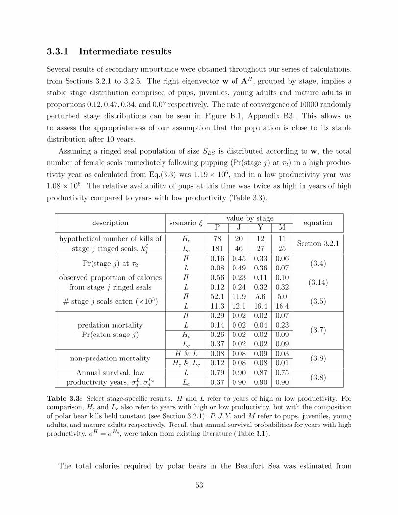
3.3.1 Intermediate results

Several results of secondary importance were obtained throughout our series of calculations,

from Sections 3.2.1 to 3.2.5. The right eigenvector w of AH , grouped by stage, implies a

stable stage distribution comprised of pups, juveniles, young adults and mature adults in

proportions 0.12, 0.47, 0.34, and 0.07 respectively. The rate of convergence of 10000 randomly

perturbed stage distributions can be seen in Figure B.1, Appendix B3. This allows us

to assess the appropriateness of our assumption that the population is close to its stable

distribution after 10 years.

Assuming a ringed seal population of size SBS is distributed according to w, the total

number of female seals immediately following pupping (Pr(stage j) at τ2) in a high produc-

tivity year as calculated from Eq.(3.3) was 1.19 × 106, and in a low productivity year was

1.08 × 106. The relative availability of pups at this time was twice as high in years of high

productivity compared to years with low productivity (Table 3.3).

description scenario ξvalue by stage

equationP J Y M

hypothetical number of kills of Hc 78 20 12 11Section 3.2.1

stage j ringed seals, kξj Lc 181 46 27 25

Pr(stage j) at τ2H 0.16 0.45 0.33 0.06

(3.4)L 0.08 0.49 0.36 0.07

observed proportion of calories H 0.56 0.23 0.11 0.10(3.14)

from stage j ringed seals L 0.12 0.24 0.32 0.32

# stage j seals eaten (×103)H 52.1 11.9 5.6 5.0

(3.5)L 11.3 12.1 16.4 16.4H 0.29 0.02 0.02 0.07

(3.7)predation mortality L 0.14 0.02 0.04 0.23Pr(eaten|stage j) Hc 0.26 0.02 0.02 0.09

Lc 0.37 0.02 0.02 0.09

non-predation mortalityH & L 0.08 0.08 0.09 0.03

(3.8)Hc & Lc 0.12 0.08 0.08 0.01

Annual survival, low L 0.79 0.90 0.87 0.75(3.8)

productivity years, σLj , σ

Lcj Lc 0.37 0.90 0.90 0.90

Table 3.3: Select stage-specific results. H and L refer to years of high or low productivity. Forcomparison, Hc and Lc also refer to years with high or low productivity, but with the compositionof polar bear kills held constant (see Section 3.2.1). P, J, Y, and M refer to pups, juveniles, youngadults, and mature adults respectively. Recall that annual survival probabilities for years with highproductivity, σH = σHc , were taken from existing literature (Table 3.1).

The total calories required by polar bears in the Beaufort Sea was estimated from

53

Eq.(3.13) to be 11.49 × 109 kcals per year. With our assumption that 2/3 of their calo-

ries come from ringed seals (θRS in Table 3.2), and then that half of that quantity from

females, this implies that 3.83× 109 calories are obtained by polar bears from female ringed

seals. In years of high productivity, ringed seal pups make up the majority of the polar bears’

intake, whether measured in calories or absolute numbers. In years with low productivity,

this shifts to the two adult stages (Table 3.3).

We calculated the predation mortality probability for seals in each stage (Table 3.3).

Combining these estimates of predation mortality and total survival probabilities in high

productivity years, we estimated non-predation mortality (Table 3.3). From these estimates

of predation and non-predation mortality in low productivity years, we estimated total sur-

vival in low productivity years (Table 3.3). Compared with high productivity years, years

with low productivity showed increased survival probabilities for pups, and decreased sur-

vival for all other stages, most notably for mature adults (Table 3.3). In contrast, performing

the same calculations for the comparison case with constant kill proportions resulted in lower

pup survival in years with reduced pup production, and constant survival of the other stages.

3.3.2 Polar bear stage-specific selection results

To address Question 1 (Figure 3.1), we calculated prey selection (Eq.(3.9)) by polar bears

on each ringed seal stage in years of both high and low productivity for both observed and

comparison kill proportions (Figure 3.3). Selection was highest for pups in high productivity

years, and mature adults in low productivity years. By comparison, if the kill composition

was held constant across years, selection for pups doubled in years with low ringed seal

productivity.

3.3.3 Matrix population model results

To address Question 2 (Figure 3.1), we analysed matrix population models both with con-

stant environments and with a periodic environment. The growth rate for a constant en-

vironment with high ringed seal productivity was log λH = 0.021 (and since AH = AHc ,

log λHc = log λH). In a constant low productivity environment, log λL = −0.046, which is

slightly higher than the comparison case log λLc = −0.064.

The annual growth rate in the periodic environment was (1/10) log λB = 0.0147, which

was slightly lower than that of the comparison case, (1/10) log λBc = 0.0151. The long-term

proportions of each stage, according to the periodic model, ranged from 0.07-0.12 for pups,

0.45-0.51 for juveniles, 0.34-0.36 for young adults, and mature adults are between 0.059-0.068

(Figure B.2, Appendix B3).

54

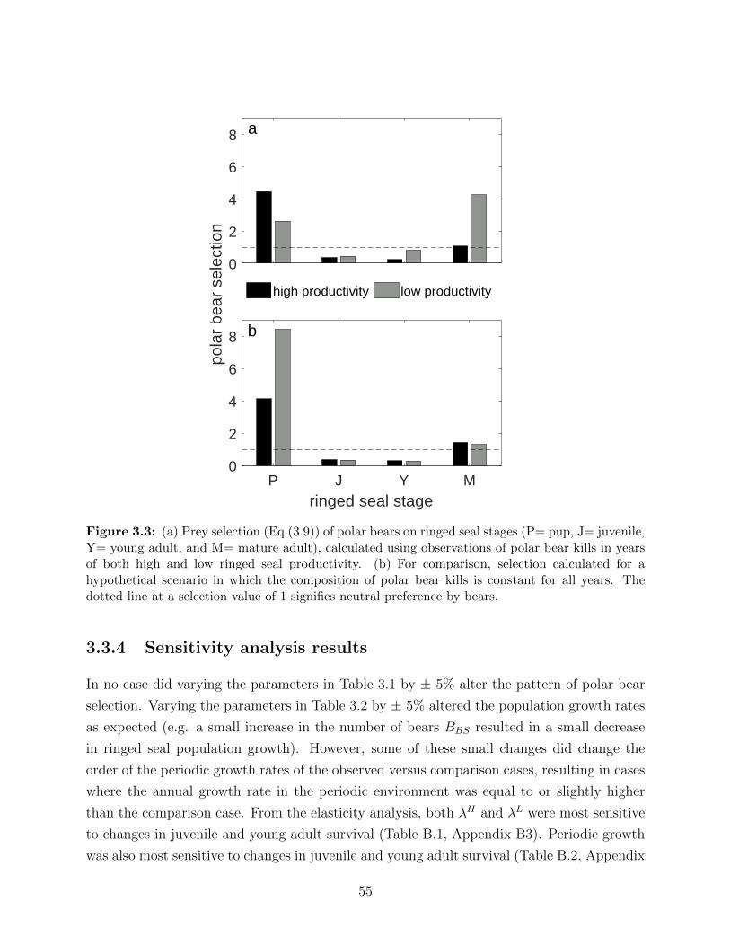
0

2

4

6

8

high productivity low productivity

P J Y Mringed seal stage

0

2

4

6

8

pola

r be

ar s

elec

tion

b

a

Figure 3.3: (a) Prey selection (Eq.(3.9)) of polar bears on ringed seal stages (P= pup, J= juvenile,Y= young adult, and M= mature adult), calculated using observations of polar bear kills in yearsof both high and low ringed seal productivity. (b) For comparison, selection calculated for ahypothetical scenario in which the composition of polar bear kills is constant for all years. Thedotted line at a selection value of 1 signifies neutral preference by bears.

3.3.4 Sensitivity analysis results

In no case did varying the parameters in Table 3.1 by ± 5% alter the pattern of polar bear

selection. Varying the parameters in Table 3.2 by ± 5% altered the population growth rates

as expected (e.g. a small increase in the number of bears BBS resulted in a small decrease

in ringed seal population growth). However, some of these small changes did change the

order of the periodic growth rates of the observed versus comparison cases, resulting in cases

where the annual growth rate in the periodic environment was equal to or slightly higher

than the comparison case. From the elasticity analysis, both λH and λL were most sensitive

to changes in juvenile and young adult survival (Table B.1, Appendix B3). Periodic growth

was also most sensitive to changes in juvenile and young adult survival (Table B.2, Appendix

55

B3).

3.4 Discussion

Theories of prey selection, prey vulnerability, population stability, and optimal foraging are

common in ecology. Prey switching integrates these concepts, but consistent experimental

evidence of the phenomenon is difficult to come by (Murdoch, 1969; Sherratt and Harvey,

1993). This study suggests a novel type of prey switching - intraspecific prey switching - by

comparing changes in the ringed seal stages selected by polar bears in the presence of high

and low ringed seal pup availability.

Our main finding was that polar bears selected most heavily for pups and mature seals

(as compared with juveniles and young adults) in both high and low productivity years. This

finding supports the idea that these stages are the most vulnerable to predation. The change

in polar bear prey selection from typical years to years with low ringed seal productivity is

suggestive of an intraspecific prey-switching behaviour, where polar bears select for seal pups

when they are more abundant, but then display a preference for older ringed seals in years

with reduced pup availability. Note that here we use the word preference in its broadest

sense, meaning only that the predator consumes proportionately more of one prey type than

would be expected given its abundance relative to other available prey, rather than implying

a conscious choice made by the predator.

Spatial separation of prey has been proposed as one mechanism leading to prey switching

(Hubbard et al., 1982) and may explain the predator preference observed in this study. The

switch from selecting for pups to older adult seals in years with low ringed seal productivity

may result from spatial segregation of ringed seals in different stages during the spring (Smith

and Stirling, 1975; Smith, 1987). In years with low ringed seal productivity, polar bears may

leave the fast ice where ringed seal pups would be found and try their chances with larger,

older seals around the ice edge or on the pack ice, where they are more likely to be found.

A natural testing of this hypothesis would be to use polar bear telemetry data to look for a

shift from landfast ice to more active ice during spring in years where ringed seals are known

to have had low productivity.

In this system, the change in polar bear prey selection reduces the ringed seal population

growth rate, though the effect size is small. Compared to the null comparison scenario, this

intraspecific switching does, however, result in a larger cohort coming from the year with

low productivity by allowing more of the pups to survive by reducing predation pressure

on pups. Our null hypothesis was that in years with fewer pups, the pups which are born

would experience higher than usual predation. This null hypothesis, explored using the

56

comparative case with constant prey composition, resulted in the expected reduction in

annual pup survival σLcP in low productivity years.

Our estimate of population growth in a constant environment with high ringed seal

productivity (log λH = 0.021) was slightly lower than two existing estimates for populations

with reduced predation pressure, as we would expect. Baltic ringed seals, a population

which does not experience predation from polar bears, have an estimated growth rate of

0.045 (Sundqvist et al., 2012). The growth rate of a hypothetical, non-harvested population

of ringed seals in the eastern Canadian Arctic was estimated to be 0.0629 (Law, 1979).

The periodic comparison model with constant kill proportions predicted slightly higher

population growth than the model with switching. This was in spite of the fact that λL >

λLC . In addition to cycles of length 10, we also considered cycles ranging in length from

6 to 12 years, with one low productivity year per cycle. This result was robust to changes

in cycle length; in each case, the comparison model had higher population growth than

the model with switching. This non-intuitive result can be explained by considering the

stage distribution available to polar bears in the spring. Ringed seal pup numbers are

severely reduced in years with low productivity, so even though our results suggest that

survival is higher for the pups that are born, this only affects a few individuals, all of which

are years away from reproductive maturity. The hypothetical scenario with constant polar

bear kill proportions results in reduced pup survival, but the survival of mature adults is

higher. These gains in survival probabilities affect individuals who are already contributing

to the population through reproduction. While not a large effect, this result highlights

the importance of considering environmental sequences as a whole rather than each year in

isolation.

Several of our results from the intermediate calculations may be compared to previously

published estimates. The annual caloric requirements for the southern Beaufort Sea polar

bear population (1800 polar bears) have elsewhere been estimated to be ≈ 4.25× 109 kcals

(Stirling and Øritsland, 1995). Scaled for a population of size BBS, the corresponding es-

timate is ≈ 7.1 × 109 kcals per year. Our estimate is approximately 1.6 times that value,

which is unsurprising given that our polar bear metabolic rate estimates are ≈ 1.6 times

larger than previous estimates (Pagano et al., 2018). In a typical year with high ringed seal

productivity, we estimated that polar bears consume 7% (by number) of the ringed seal pop-

ulation. This is below the range of 14.5–27.5% calculated by Stirling and Øritsland (1995),

though they admitted their behavioural method may have overestimated the number of seals

consumed by polar bears (Stirling and Øritsland, 1995). Our calculation that 29% of ringed

seal pups are predated in a typical year falls within the range of 8–44% supplied by Hammill

and Smith (1991).

57

The stable age distribution predicted from matrix AH had the lowest proportion of seals

as pups (12%) and the highest proportion as juveniles (47%), with the remainder falling

in the two adult stages (36%). Visual assessment of the convergence of a broad range of

perturbed distributions (Figure B.1, Appendix B3) provided satisfactory evidence that the

population would be distributed approximately according to its stable stage distribution 10

years after a perturbation. We would expect the stable age distribution to be reflected in the

proportions found during the subsistence open-water harvest, when seals are assumed to be

homogeneously distributed and equally susceptible to harvesting (Holst et al., 1999; Smith,

1973). Our values are consistent with samples from harvested populations documented by

Smith (1987), who reported 15, 54, and 31%, for pups, juveniles, and adults respectively,

as well as Smith (1973), who reported 12, 44, and 43% respectively. Our calculated pro-

portions vary from the harvest proportions reported by Harwood et al. (2012), but those

values - 21, 14, and 66% for pups, juveniles, and adults - were taken from harvest samples

collected earlier in the summer when sampling may have been biased by spatial segregation

of seals during breakup when juveniles are thought to be highly mobile, migrating to find

high quality foraging habitat (Freitas et al., 2008a). The consistency between our model

and observed harvest values provides further justification for assuming the population is dis-

tributed approximately according to the stable distribution prior to a year with anomalously

late breakup.

We did not consider possible shifts by polar bears to alternative prey species. While

species diversity is lower in the eastern Beaufort Sea than in other Arctic regions, polar

bears in this region are known to also prey on bearded seals (Erignathus barbatus) (Pilfold

et al., 2012; Stirling, 2002). They may derive a more significant part of their diet from

bearded seals to compensate for reductions in the ringed seal population, provided bearded

seals do not experience the same years of reduced productivity.

It has also been suggested that in years with low ringed seal productivity, polar bear pop-

ulations show signs of stress (reduced numbers, reduced reproductive rates), suggesting that

they may consume less energy overall (Stirling and Archibald, 1977; Stirling and Øritsland,

1995; Stirling and Lunn, 1997). Polar bears may also display increased fasting behaviour in

response to reduced ringed seal abundance (Cherry et al., 2009; Rode et al., 2018). We also

did not consider the effects of fox predation on the ringed seal population. The effects of this

may be significant in some years in the Beaufort Sea (Kelly et al., 2010; Smith, 1987; Smith

et al., 1991), but the timing and causes of surges in fox populations are not well understood.

Being a cryptic species, several of the parameter estimates required for our ringed seal

population model were not precisely known. The qualitative nature of the selection results

was insensitive to small changes (± 5%) in parameter values, and the response was simply to

58

either reduce or increase predation pressure on ringed seals in an intuitive way. While small

parameter changes did result in changes when comparing the periodic population growth rate

to that of the comparison model, the magnitude of the difference between these scenarios

remained small, emphasizing the point that this behaviour has negligible effect - positive

or negative - on the ringed seal population. We also only presented results for one year of

reduced ringed seal production per decade. We expect that an extension of our model to

include a second or third consecutive year of reduced pup production would yield no new

insight and serve only to marginally lower the population growth rate.

One of the reasons that prey switching is difficult to show empirically is that prey switch-

ing may occur at one prey density but not at another (Murdoch, 1969). We could not explore

this possibility here, and similarly could not tease out the effects of relative frequency from

absolute frequency. Further, we have only discussed the functional response of the predator

(i.e., how the number of prey in each stage eaten changes with prey density) rather than

the numerical response of the predator. We have held the predator population size constant

across years, which we feel is justifiable when considering short transient periods of reduced

ringed seal productivity.

This study explored this predator-prey system as it was observed over the previous several

decades. Since then, the polar bear population in the southern Beaufort Sea has declined

(Bromaghin et al., 2015), which we would expect to result in reduced predation pressure on

ringed seals. Looking ahead, as the climate warms, the Arctic climatic cycles of the past

century are likely to change both in frequency and intensity (Proshutinsky et al., 2015).

Environmental fluctuations which affect both predator and prey populations add complexity

and nonlinearities to the effects of environmental changes. The response of either prey

or predator to both climatic fluctuations and the response of the other could conceivably

mitigate or exacerbate anticipated effects of climate change (Wilmers et al., 2007). Over

the coming decades, years with low ringed seal productivity due to heavy winter ice cover

and late ice breakup may no longer occur with the same frequency or severity (Kelly et al.,

2010). Instead, increased frequency of years with anomalously early breakup may introduce

new stresses on ringed seal populations. While this is also believed to have a negative affect

on ringed seal productivity, the mechanism is different, resulting not from low pregnancy

rates in females, but from low pup survival rates (Ferguson et al., 2005; Kelly et al., 2010).

How the diet composition of polar bears will respond to these changes remains to be seen.

We have explored how the diet composition of polar bears may have shifted in response

to short term fluctuations in the structure of their prey populations. Spatial segregation of

different stages within the ringed seal population provides the most likely explanation for

the intraspecific switching type behaviour. While the implications for polar bears, such as

59

associated changes in foraging habitat or increases in hunting effort, may warrant further

investigation, the effects on the population growth of their prey appear minor.

Appendices

B1 Parameter notes

σHi

Stage-specific survival probabilities are not well known for ringed seals. Considerable varia-

tion exists between regions, studies, and calculation methodologies. Smith (1987) calculated

annual age-specific survival probabilities from a smoothed age-distribution obtained from the

summer harvest in the Beaufort Sea. Survival probabilities obtained in this way (with simple

averages taken from Table 25 in (Smith, 1987) to obtain values for each stage) are 0.84, 0.86,

and 0.85 for pups, juveniles, and adults, respectively. Survival probabilities obtained from

harvest data in this way are notoriously unreliable, however, as they assume that the popu-

lation was at a stable distribution at the time of sampling (Smith, 1987). Other studies have

estimated annual pup survival to be markedly lower; 0.61 (Smith, 1973), 0.65 (Sundqvist

et al., 2012), and 0.69 (McLaren, 1958). Estimates of pup survival are complicated by large

fluctuations in fox predation pressure (Burns et al., 1982; Lydersen and Gjertz, 1986; Smith,

1987). Some studies have also suggested increasing mortality for older seals (Smith, 1973).

The values in our demographic model for typical high productivity years are informed by

the synthesis of studies presented by Kelly et al. (2010) and chosen to be at the upper end

of those ranges.

mi

The chosen rates for the expected number of female offspring produced in a typical year mGi

are comparable to that found elsewhere in the literature, with values increasing from very

low at age 4 to approximately 0.4 by age 10 (Hammill, 1987; Smith, 1973). In the absence

of consensus on the topic (see (Kelly et al., 2010) for a brief review of the evidence), we do

not include sexual senescence in our reproductive rates.

meeη

The metabolic energetic equivalent meeη of a bear in each stage η is a scaling factor based on

life history stage and sex which standardizes the energetic requirements of each bear relative

to that of a solitary adult female (Regehr et al., 2015). The eight bear life history stages

60

(values of η) are cubs of the year, yearlings, 2 year-old females and males, subadult females

and males, and adult females and males. The metabolic energetic equivalents for each stage

are 0.2, 0.6, 0.7, 0.9, 0.8, 1, 1, and 1.3, respectively.

pη

We use estimates of the age structure of the SB bear population (Table 3 in Stirling and

Øritsland (1995)) and assume that this structure is appropriate for the entire study region

(recall the Beaufort Sea area is comprised of the Northern and Southern Beaufort polar bear

subpopulations). We group the number of bears of each age into stages matching those of

Regehr et al. (2015). This results in a polar bear population comprised of 10.6% cubs of the

year, 9.9% yearlings, 4.6% 2 year-old females, 4.6% 2 year-old males, 8% subadult females,

8.1% subadult males, 27.2% adult females, and 27% adult males.

FMR

To obtain an average daily FMR value over the year, we used an estimate of 12,324.7 kcal

day−1 throughout the part of the year where bears are actively hunting on the sea ice, and

8861.2 kcal day−1 per day for the approximately 100 days in summer when bears are fasting

(Pagano et al., 2018), combining these estimates to obtain an average value of 11375.8 kcal

day−1 over the whole year.

kHj , kLj

Observed ringed seal kills for years of typical and low ringed seal productivity may be seen

in Figure 3 of Pilfold et al.(2012). Exact values were obtained through communication with

the authors. Note that sample sizes of adult ringed seals killed by bears were low in years

with typical ice conditions, and aging to determine whether an adult should be classified as

a young or mature adult was not done for all seals. We follow the findings of Pilfold et al.

(2012) and assume that the ratio of young adult (< 21) to mature (≥ 21) adult seal kills is

approximately unity.

Stirling and Øritsland (1995) assumed a constant stage composition of polar bear kills

across years, with a similar distribution (61% pups, 22% juveniles, and 17% adults) to that

found in high productivity years by Pilfold et al. (2012).

calj

We have chosen to use the same values as in Stirling and Øritsland (1995): pups initially

provide approximately 10000 kcals (Apr 1-15), then 50000 kcals (Apr 16-30), and finally

61

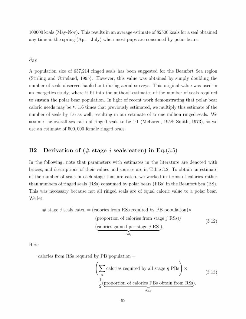
100000 kcals (May-Nov). This results in an average estimate of 82500 kcals for a seal obtained

any time in the spring (Apr - July) when most pups are consumed by polar bears.

SBS

A population size of 637,214 ringed seals has been suggested for the Beaufort Sea region

(Stirling and Øritsland, 1995). However, this value was obtained by simply doubling the

number of seals observed hauled out during aerial surveys. This original value was used in

an energetics study, where it fit into the authors’ estimates of the number of seals required

to sustain the polar bear population. In light of recent work demonstrating that polar bear

caloric needs may be ≈ 1.6 times that previously estimated, we multiply this estimate of the

number of seals by 1.6 as well, resulting in our estimate of ≈ one million ringed seals. We

assume the overall sex ratio of ringed seals to be 1:1 (McLaren, 1958; Smith, 1973), so we

use an estimate of 500, 000 female ringed seals.

B2 Derivation of (# stage j seals eaten) in Eq.(3.5)

In the following, note that parameters with estimates in the literature are denoted with

braces, and descriptions of their values and sources are in Table 3.2. To obtain an estimate

of the number of seals in each stage that are eaten, we worked in terms of calories rather

than numbers of ringed seals (RSs) consumed by polar bears (PBs) in the Beaufort Sea (BS).

This was necessary because not all ringed seals are of equal caloric value to a polar bear.

We let

# stage j seals eaten = (calories from RSs required by PB population)×

(proportion of calories from stage j RSs)/

(calories gained per stage j RS⏞ ⏟⏟ ⏞calj

).(3.12)

Here

calories from RSs required by PB population =(∑η

calories required by all stage η PBs

)×

1

2(proportion of calories PBs obtain from RSs⏞ ⏟⏟ ⏞

θRS

),

(3.13)

62

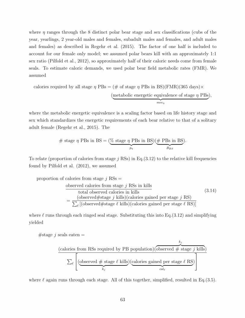
where η ranges through the 8 distinct polar bear stage and sex classifications (cubs of the

year, yearlings, 2 year-old males and females, subadult males and females, and adult males

and females) as described in Regehr et al. (2015). The factor of one half is included to

account for our female only model; we assumed polar bears kill with an approximately 1:1

sex ratio (Pilfold et al., 2012), so approximately half of their caloric needs come from female

seals. To estimate caloric demands, we used polar bear field metabolic rates (FMR). We

assumed

calories required by all stage η PBs = (# of stage η PBs in BS)(FMR)(365 days)×

(metabolic energetic equivalence of stage η PBs⏞ ⏟⏟ ⏞meeη

),

where the metabolic energetic equivalence is a scaling factor based on life history stage and

sex which standardizes the energetic requirements of each bear relative to that of a solitary

adult female (Regehr et al., 2015). The

# stage η PBs in BS = (% stage η PBs in BS⏞ ⏟⏟ ⏞pη

)(# PBs in BS⏞ ⏟⏟ ⏞BBS

).

To relate (proportion of calories from stage j RSs) in Eq.(3.12) to the relative kill frequencies

found by Pilfold et al. (2012), we assumed

proportion of calories from stage j RSs =

observed calories from stage j RSs in kills

total observed calories in kills

=(observed#stage j kills)(calories gained per stage j RS)∑ℓ [(observed#stage ℓ kills)(calories gained per stage ℓ RS)]

(3.14)

where ℓ runs through each ringed seal stage. Substituting this into Eq.(3.12) and simplifying

yielded

#stage j seals eaten =

(calories from RSs required by PB population)(

kj⏟ ⏞⏞ ⏟observed # stage j kills)

∑ℓ

⎡⎣(observed # stage ℓ kills⏞ ⏟⏟ ⏞kj

)(calories gained per stage ℓ RS⏞ ⏟⏟ ⏞calℓ

)

⎤⎦where ℓ again runs through each stage. All of this together, simplified, resulted in Eq.(3.5).

63

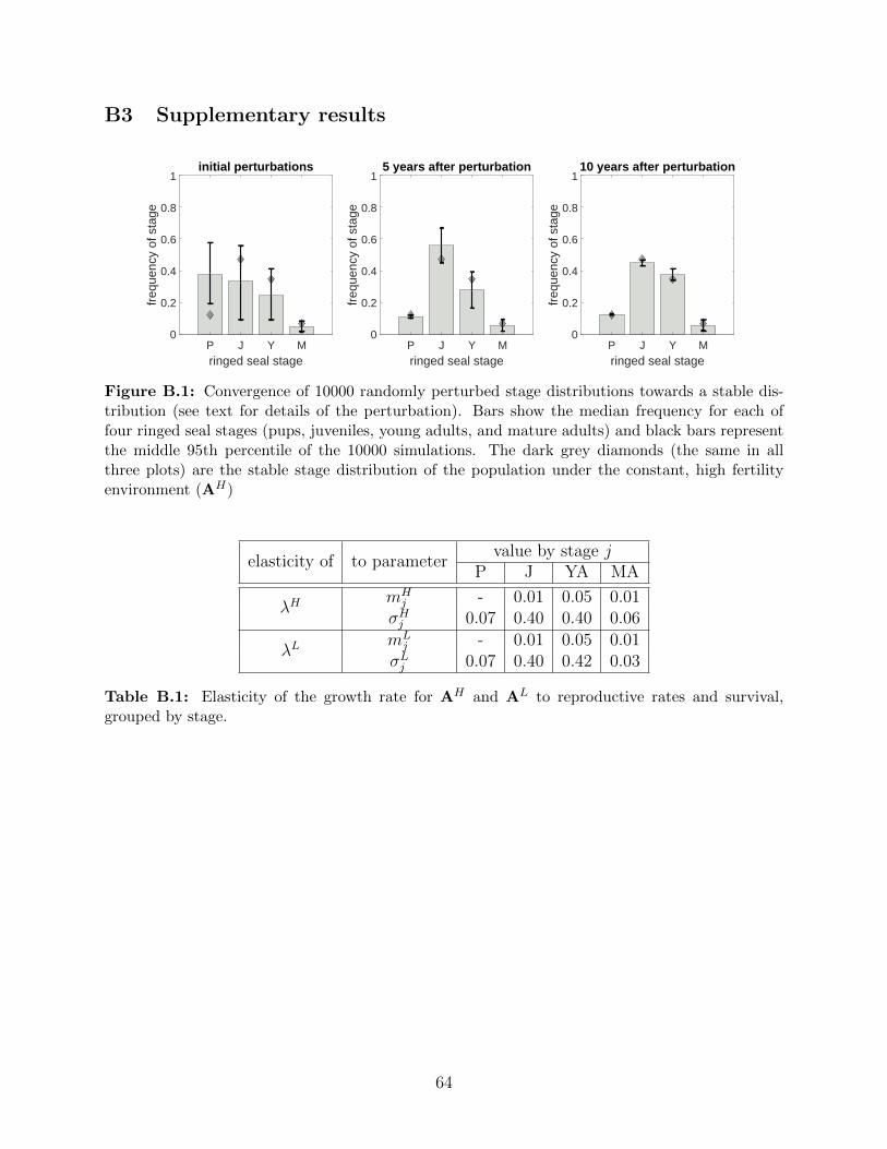
B3 Supplementary results

initial perturbations

P J Y Mringed seal stage

0

0.2

0.4

0.6

0.8

1

freq

uenc

y of

sta

ge5 years after perturbation

P J Y Mringed seal stage

0

0.2

0.4

0.6

0.8

1

freq

uenc

y of

sta

ge

10 years after perturbation

P J Y Mringed seal stage

0

0.2

0.4

0.6

0.8

1

freq

uenc

y of

sta

ge

Figure B.1: Convergence of 10000 randomly perturbed stage distributions towards a stable dis-tribution (see text for details of the perturbation). Bars show the median frequency for each offour ringed seal stages (pups, juveniles, young adults, and mature adults) and black bars representthe middle 95th percentile of the 10000 simulations. The dark grey diamonds (the same in allthree plots) are the stable stage distribution of the population under the constant, high fertilityenvironment (AH)

elasticity of to parametervalue by stage j

P J YA MA

λHmH

j - 0.01 0.05 0.01σHj 0.07 0.40 0.40 0.06

λLmL

j - 0.01 0.05 0.01σLj 0.07 0.40 0.42 0.03

Table B.1: Elasticity of the growth rate for AH and AL to reproductive rates and survival,grouped by stage.

64

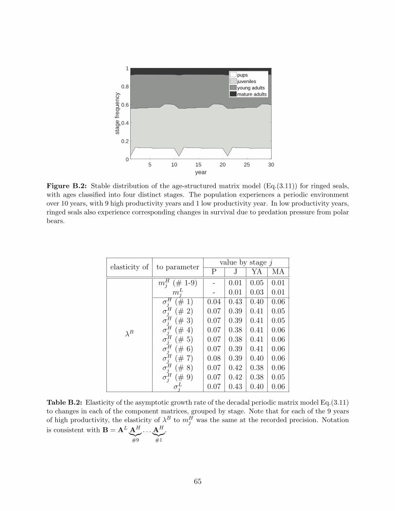
5 10 15 20 25 30year

0

0.2

0.4

0.6

0.8

1

stag

e fr

eque

ncy

pupsjuvenilesyoung adultsmature adults

Figure B.2: Stable distribution of the age-structured matrix model (Eq.(3.11)) for ringed seals,with ages classified into four distinct stages. The population experiences a periodic environmentover 10 years, with 9 high productivity years and 1 low productivity year. In low productivity years,ringed seals also experience corresponding changes in survival due to predation pressure from polarbears.

elasticity of to parametervalue by stage j

P J YA MA

λB

mHj (# 1-9) - 0.01 0.05 0.01mL

j - 0.01 0.03 0.01σHj (# 1) 0.04 0.43 0.40 0.06σHj (# 2) 0.07 0.39 0.41 0.05σHj (# 3) 0.07 0.39 0.41 0.05σHj (# 4) 0.07 0.38 0.41 0.06σHj (# 5) 0.07 0.38 0.41 0.06σHj (# 6) 0.07 0.39 0.41 0.06σHj (# 7) 0.08 0.39 0.40 0.06σHj (# 8) 0.07 0.42 0.38 0.06σHj (# 9) 0.07 0.42 0.38 0.05σLj 0.07 0.43 0.40 0.06

Table B.2: Elasticity of the asymptotic growth rate of the decadal periodic matrix model Eq.(3.11)to changes in each of the component matrices, grouped by stage. Note that for each of the 9 yearsof high productivity, the elasticity of λB to mH

j was the same at the recorded precision. Notation

is consistent with B = AL AH⏞⏟⏟⏞#9

. . . AH⏞⏟⏟⏞#1

.

65

Chapter 4

Modelling optimal responses and

fitness consequences in a changing

Arctic

The work presented in this chapter has been submitted and is under review as: Reimer,

J.R., Mangel, M., Derocher, A.E., and Lewis, M.A. Modelling optimal responses and fitness

consequences in a changing Arctic.

4.1 Introduction

Natural selection acts across several interacting processes, including survival, mate-finding,

foraging, and reproduction. Individuals must balance a series of tradeoffs, whether through

behavioural means or physiological adaptations. For example, an individual may need to

choose between two possible foraging patches, taking into account the food available as well

as the risk of predation in each patch (Holbrook and Schmitt, 1988; Ludwig and Rowe, 1990).

Similarly, tradeoffs between the quantity and viability of offspring determine optimal clutch

size (Lack, 1947; Mangel et al., 1995). Natural selection favours individuals with higher

fitness (here defined as an individual’s expected lifetime reproductive success) resulting from

successfully balancing these competing factors. Optimality theory aims to identify an in-

dividual’s optimal decision in light of a set of rewards, risks, and constraints. Decisions,

in this context, may refer to conscious behavioural choices or to subconscious physiological

responses. Optimal decisions need not be the same for every individual at each time; each

individual may be in one of several relevant states (e.g., their energetic state, reproductive

state, or age) that may affect the decisions available to the individual, outcomes that are

66

possible, as well as which decision is optimal. While these optimal adaptations may not be

perfectly achieved, framing questions in this way provides insight into the competing forces

faced by an individual (Parker and Smith, 1990).

Polar bears (Ursus maritimus) of different sexes and in different reproductive states vary

in their choice of foraging habitat during the spring feeding period (Stirling et al., 1993;

Pilfold et al., 2014a). Sea ice habitat used by polar bears in the southern Beaufort Sea can

be broadly grouped into two types: active ice and landfast ice (Stirling et al., 1993). Active

ice, including pack ice and the flow edge, is high quality polar bear foraging habitat with

abundant prey, namely ringed seals (Pusa hispida) and bearded seals (Erignathus barbatus)

(Stirling et al., 1993). Near shore, landfast ice provides lower quality foraging habitat, with

the main available prey being naive but small ringed seal pups and their mothers (Smith

and Stirling, 1975). Male polar bears of all ages and females who are not accompanied

by dependent offspring are found primarily in the active ice (Stirling et al., 1993). Female

polar bears accompanied by dependent offspring (especially females with cubs-of-the-year,

COYs), however, are found more often in the landfast ice (Stirling et al., 1993). This is

thought to result from a risk avoidance strategy (Pilfold et al., 2014a); cubs may be at risk

of cannibalism (Derocher and Wiig, 1999; Amstrup et al., 2006) or hypothermia due to the

swimming that may be necessary in more active ice (Blix and Lentfer, 1979; Monnett and

Gleason, 2006). Stirling et al. (1993) found that females with COYs in the southern Beaufort

Sea were nearly twice as likely to be in fast ice as expected.

In addition to the foraging decisions made on daily timescales, female polar bears also

make facultative reproductive decisions. Female polar bears mate in the spring, but delay

implantation until the autumn (Lønø, 1970; Ramsay and Stirling, 1988). If her energy

reserves are too low at this time, a female polar bear may abort the pregnancy rather

than continuing to deplete her reserves (Derocher et al., 1992; Atkinson and Ramsay, 1995).

Similarly, if her energy reserves are sufficiently depleted while she still has dependent cubs,

the quality of her milk will decline and eventually cease entirely, which may result in cub

mortality (Derocher et al., 1993; Molnar et al., 2009). The level of energy reserves at which

it may be optimal for her to stop investing in her current reproductive attempt are unknown.

In recent decades, the ice free season has increased approximately 10–20 days per decade

across the southern Beaufort Sea (Parkinson, 2014). For polar bears, this results in a shorter

feeding season over which they must attempt to acquire the necessary reserves to survive

the longer summer fasting season (Pongracz and Derocher, 2017). These changing ice condi-

tions have already been linked with smaller body size, reduced recruitment, and population

declines in the Beaufort Sea (Hunter et al., 2010; Regehr et al., 2010; Rode et al., 2010a).

What is known about polar bears’ preferred foraging habitat has been studied within

67

a framework of selection (i.e., habitat use versus relative availability) (Stirling et al., 1993;

Durner et al., 2009) or species distribution models (Pilfold et al., 2014a). We took a different

approach, using optimality theory to explore conditions under which the energetic require-

ments and vulnerability of bears in different life history stages may explain their observed

spatial segregation. We then used our model to explore the implications of changes in the

timing of spring sea ice breakup for polar bear foraging decisions and, ultimately, individual

fitness. This framework also allowed us to estimate the energetic thresholds at which it

would be optimal for a female polar bear to abort her pregnancy or cease lactation.

We desired a modelling framework that would allow for a high degree of flexibility in the

stochastic nature of the model components as well as the feedback between the controls and

the state. For this, the discrete nature and flexibility of stochastic dynamic programming

(SDP) offers a convenient framework (Clark and Mangel, 2000; Houston and McNamara,

1999). SDP models, also known as dynamic state variable models, are individual based

models used to determine optimal decisions, given a known objective and constraints (Clark

and Mangel, 2000). These models have been used for a variety of purposes, such as determin-

ing the optimal overwintering habitat of elk (Cervus canadensis) (Noonburg et al., 2007), the

conditions under which a predator with distinct predation strategies is predicted to switch

between them (Dukas and Clark, 1995), and the effects of acoustic and other anthropogenic

disturbances on marine mammals (Schwarz et al., 2016; McHuron et al., 2017).

We created an SDP model for an individual female polar bear over her entire adult

lifetime, from sexual maturity until death (for other examples of SDP models spanning

adulthood, see Marrow et al. (1996); McHuron et al. (2018)). SDP allows integration of the

bear’s need to balance tradeoffs between energy gain, reproduction, and cub survival (Clark

and Mangel, 2000). The classical SDP patch choice model optimizes the patch choice of an

individual who may inhabit different environments, each with different risks and rewards,

over a short time frame. Our model is an extension of this, maximizing the individual’s

recruited offspring over her entire lifetime and including a variable reproductive state which

is, itself, subject to optimization.

Model outputs are (1) her expected future fitness throughout her lifetime, and (2) a set

of optimal decisions, dependent on energetic and reproductive state. The optimal decisions

fall into two main categories: (i) during each spring, the daily optimal foraging patch (active

ice or fast ice), and (ii) at the end of each spring, the decision, when relevant, whether to

abort or continue a pregnancy, or whether to continue or cease milk production. We use

this model to answer 3 questions: (1) How much added risk of mortality in the active ice

would result in predictions of optimal habitat use similar to those observed? (2) What is the

energetic threshold below which it is optimal for a female to abort her pregnancy or cease

68

lactation? (3) What changes in foraging habitat selection and reproductive behaviour do we

predict if the spring feeding season is shortened, and the summer fasting period similarly

lengthened, and what would be the resultant changes in her fitness?

4.2 Methods

We considered two possible spring foraging habitats, with an individual female making a

daily decision to forage in either active or fast ice. The bear must choose where to forage

based on the probability of finding and catching prey, the expected energetic returns of

that prey, and the risk in each patch, which may depend on the bear’s reproductive state.

Parameter values and functional forms are in Table 4.1.

Our model included two state variables: x(t, n), the energy reserves (MJ) of the bear,

and η(t, n), the bear’s reproductive state, both at time t in the nth year of her adult life. We

assumed death from starvation when her energy reserves fall to the critical level xcrit, and

an upper bound xmax on her reserves, so xcrit ≤ x ≤ xmax. Female polar bears may take one

of four reproductive states, η ∈ {1, 2, 3, 4}, corresponding to single, pregnant, with a litter

of 1 or more COYs, and with a litter of 1 or more yearlings. Polar bears in the Beaufort Sea

give birth to a litter of 1 to 3 cubs which remain with their mother until they are weaned.

Weaning typically occurs in the spring of their second year, so a female may successfully

wean a litter every 3 years at most (Ramsay and Stirling, 1988).

The time interval of our SDP routine was one day, resulting in the optimal decisions and

resultant fitness for each day of each spring. The first day of spring, tspring, coincides with

the beginning of ringed seal pupping, signifying the beginning of a period of hyperphagia

for polar bears (Stirling and McEwan, 1975; Ramsay and Stirling, 1988). During the spring,

single females may also mate. Females are available to mate for the first time at the start of

their sixth spring in the southern Beaufort Sea (approximately age 5.5, model year n = 1)

(Stirling et al., 1976; Lentfer et al., 1980). We assumed both spring feeding and mating stop

when the sea ice breaks up over the continental shelf in early summer, approximately on day

tbreakup. We designated the days between tspring and tbreakup as spring, and the SDP model

was used for each day in this period.

We assumed a maximum encounter of one prey item per day and that handling time and

prey consumption also occur within this one day window. Prey are encountered and captured

with a daily probability λi, depending on patch i ∈ {fast ice, active ice}. Upon successfully

catching prey, the bear’s energetic state increases by Yi(t), the expected energetic gain from

a seal in patch i on day t. The fast ice has lower expected daily energetic gain than the

active ice (Figure C.1, Appendix C1).

69

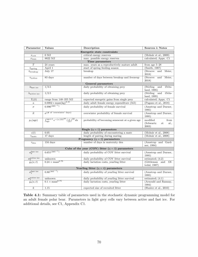
Parameter Values Description Sources & Notes

Energetic state constraintsxcrit 0 MJ critical energy reserves (Molnar et al., 2009)xmax 8822 MJ max. possible energy reserves calculated; Appx. C1

Time parametersT 24 years max. years as a reproductively mature adult from age 5–28

tspring April 1 start of spring feeding season (Smith, 1987)tbreakup July 17 breakup (Stroeve and Meier,

2018)τicefree 83 days number of days between breakup and freezeup (Stroeve and Meier,

2018)General parameters

λfast ice 1/3.5 daily probability of obtaining prey (Stirling and Ørits-land, 1995)

λactive ice 1/2.5 daily probability of obtaining prey (Stirling and Ørits-land, 1995)

Yi(t) range from 148–355 MJ expected energetic gains from single prey calculated; Appx. C1

a 0.0002 ∗mass(kg)2.41 daily adult female energy expenditure (MJ) (Pagano et al., 2018)

σ 0.996(365−1) daily probability of female survival (Amstrup and Durner,

1995)ˆσ σ(# of ‘overwinter’ days) overwinter probability of female survival (Amstrup and Durner,1995)

ps(age)∫ age+1age e−(x/23)23

(x23

)22dx probability of becoming senescent at a given age modified from

(Schwartz et al.,2003)

Single (η = 1) parametersϵ(t) 0.05 daily probability of encountering a mate (Molnar et al., 2008)τmate 17 days length of pairing during mating (Molnar et al., 2008)

Pregnancy (η = 2) parametersτden 134 days number of days in maternity den (Amstrup and Gard-

ner, 1994)Cubs of the year (COY) litter (η = 3) parameters

σfast ice0 0.651(365

−1) daily probability of COY litter survival (Amstrup and Durner,1995)

σactive ice0 unknown daily probability of COY litter survival estimated; (4.2)g3(x, t) 0.24×mass0.75 daily lactation costs, yearling litter (Gittleman and Of-

tedal, 1987)Yearling litter (η = 4) parameters

σfast ice1 0.86(365

−1) daily probability of yearling litter survival (Amstrup and Durner,1995)

σactive ice1 unknown daily probability of yearling litter survival estimated; (4.1)g4(x, t) 0.1×mass0.75 daily lactation costs, yearling litter (Arnould and Ramsay,

1994)k 1.15 expected size of recruited litter (Hunter et al., 2010)

Table 4.1: Summary table of parameters used in the stochastic dynamic programming model foran adult female polar bear. Parameters in light grey cells vary between active and fast ice. Foradditional details, see C1, Appendix C1.

70

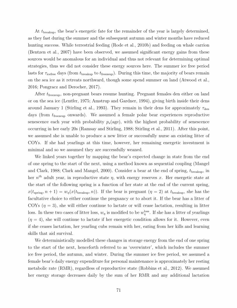
At tbreakup, the bear’s energetic fate for the remainder of the year is largely determined,

as they fast during the summer and the subsequent autumn and winter months have reduced

hunting success. While terrestrial feeding (Rode et al., 2010b) and feeding on whale carrion

(Bentzen et al., 2007) have been observed, we assumed significant energy gains from these

sources would be anomalous for an individual and thus not relevant for determining optimal

strategies, thus we did not consider these energy sources here. The summer ice free period

lasts for τicefree days (from tbreakup to tfreezeup). During this time, the majority of bears remain

on the sea ice as it retreats northward, though some spend summer on land (Atwood et al.,

2016; Pongracz and Derocher, 2017).

After tfreezeup, non-pregnant bears resume hunting. Pregnant females den either on land

or on the sea ice (Lentfer, 1975; Amstrup and Gardner, 1994), giving birth inside their dens

around January 1 (Stirling et al., 1993). They remain in their dens for approximately τden

days (from tfreezeup onwards). We assumed a female polar bear experiences reproductive

senescence each year with probability ps(age), with the highest probability of senescence

occurring in her early 20s (Ramsay and Stirling, 1988; Stirling et al., 2011). After this point,

we assumed she is unable to produce a new litter or successfully nurse an existing litter of

COYs. If she had yearlings at this time, however, her remaining energetic investment is

minimal and so we assumed they are successfully weaned.

We linked years together by mapping the bear’s expected change in state from the end

of one spring to the start of the next, using a method known as sequential coupling (Mangel

and Clark, 1988; Clark and Mangel, 2000). Consider a bear at the end of spring, tbreakup, in

her nth adult year, in reproductive state η, with energy reserves x. Her energetic state at

the start of the following spring is a function of her state at the end of the current spring,

x(tspring, n + 1) = wη(x(tbreakup, n)). If the bear is pregnant (η = 2) at tbreakup, she has the

facultative choice to either continue the pregnancy or to abort it. If the bear has a litter of

COYs (η = 3), she will either continue to lactate or will cease lactation, resulting in litter

loss. In these two cases of litter loss, wη is modified to be wlossη . If she has a litter of yearlings

(η = 4), she will continue to lactate if her energetic condition allows for it. However, even

if she ceases lactation, her yearling cubs remain with her, eating from her kills and learning

skills that aid survival.

We deterministically modelled these changes in storage energy from the end of one spring

to the start of the next, henceforth referred to as ‘overwinter’, which includes the summer

ice free period, the autumn, and winter. During the summer ice free period, we assumed a

female bear’s daily energy expenditure for personal maintenance is approximately her resting

metabolic rate (RMR), regardless of reproductive state (Robbins et al., 2012). We assumed

her energy storage decreases daily by the sum of her RMR and any additional lactation

71

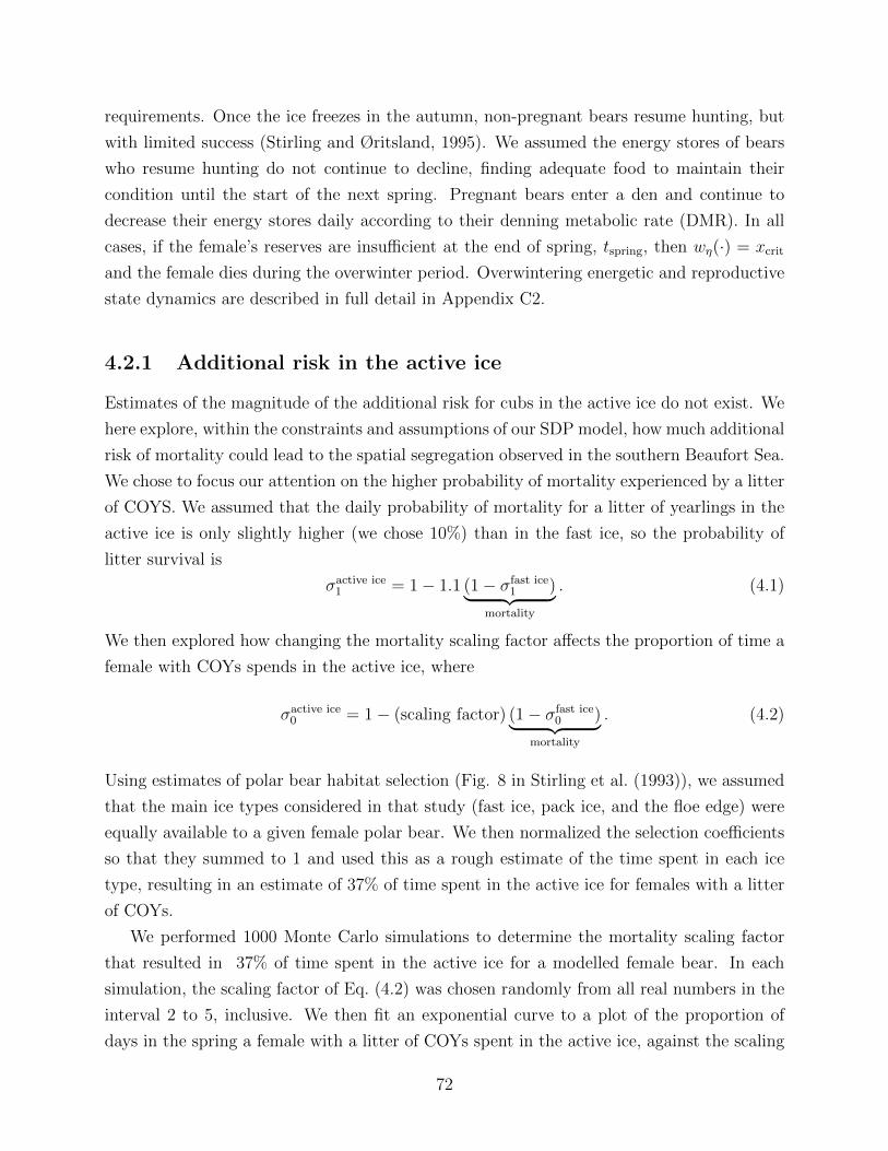
requirements. Once the ice freezes in the autumn, non-pregnant bears resume hunting, but

with limited success (Stirling and Øritsland, 1995). We assumed the energy stores of bears

who resume hunting do not continue to decline, finding adequate food to maintain their

condition until the start of the next spring. Pregnant bears enter a den and continue to

decrease their energy stores daily according to their denning metabolic rate (DMR). In all

cases, if the female’s reserves are insufficient at the end of spring, tspring, then wη(·) = xcrit

and the female dies during the overwinter period. Overwintering energetic and reproductive

state dynamics are described in full detail in Appendix C2.

4.2.1 Additional risk in the active ice

Estimates of the magnitude of the additional risk for cubs in the active ice do not exist. We

here explore, within the constraints and assumptions of our SDP model, how much additional

risk of mortality could lead to the spatial segregation observed in the southern Beaufort Sea.

We chose to focus our attention on the higher probability of mortality experienced by a litter

of COYS. We assumed that the daily probability of mortality for a litter of yearlings in the

active ice is only slightly higher (we chose 10%) than in the fast ice, so the probability of

litter survival is

σactive ice1 = 1− 1.1 (1− σfast ice

1 )⏞ ⏟⏟ ⏞mortality

. (4.1)

We then explored how changing the mortality scaling factor affects the proportion of time a

female with COYs spends in the active ice, where

σactive ice0 = 1− (scaling factor) (1− σfast ice

0 )⏞ ⏟⏟ ⏞mortality

. (4.2)

Using estimates of polar bear habitat selection (Fig. 8 in Stirling et al. (1993)), we assumed

that the main ice types considered in that study (fast ice, pack ice, and the floe edge) were

equally available to a given female polar bear. We then normalized the selection coefficients

so that they summed to 1 and used this as a rough estimate of the time spent in each ice

type, resulting in an estimate of 37% of time spent in the active ice for females with a litter

of COYs.

We performed 1000 Monte Carlo simulations to determine the mortality scaling factor

that resulted in 37% of time spent in the active ice for a modelled female bear. In each

simulation, the scaling factor of Eq. (4.2) was chosen randomly from all real numbers in the

interval 2 to 5, inclusive. We then fit an exponential curve to a plot of the proportion of

days in the spring a female with a litter of COYs spent in the active ice, against the scaling

72

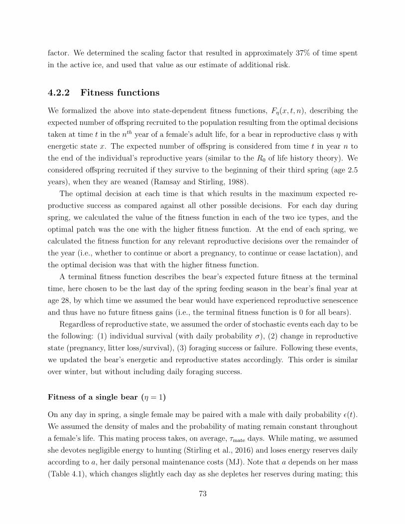
factor. We determined the scaling factor that resulted in approximately 37% of time spent

in the active ice, and used that value as our estimate of additional risk.

4.2.2 Fitness functions

We formalized the above into state-dependent fitness functions, Fη(x, t, n), describing the

expected number of offspring recruited to the population resulting from the optimal decisions

taken at time t in the nth year of a female’s adult life, for a bear in reproductive class η with

energetic state x. The expected number of offspring is considered from time t in year n to

the end of the individual’s reproductive years (similar to the R0 of life history theory). We

considered offspring recruited if they survive to the beginning of their third spring (age 2.5

years), when they are weaned (Ramsay and Stirling, 1988).

The optimal decision at each time is that which results in the maximum expected re-

productive success as compared against all other possible decisions. For each day during

spring, we calculated the value of the fitness function in each of the two ice types, and the

optimal patch was the one with the higher fitness function. At the end of each spring, we

calculated the fitness function for any relevant reproductive decisions over the remainder of

the year (i.e., whether to continue or abort a pregnancy, to continue or cease lactation), and

the optimal decision was that with the higher fitness function.

A terminal fitness function describes the bear’s expected future fitness at the terminal

time, here chosen to be the last day of the spring feeding season in the bear’s final year at

age 28, by which time we assumed the bear would have experienced reproductive senescence

and thus have no future fitness gains (i.e., the terminal fitness function is 0 for all bears).

Regardless of reproductive state, we assumed the order of stochastic events each day to be

the following: (1) individual survival (with daily probability σ), (2) change in reproductive

state (pregnancy, litter loss/survival), (3) foraging success or failure. Following these events,

we updated the bear’s energetic and reproductive states accordingly. This order is similar

over winter, but without including daily foraging success.

Fitness of a single bear (η = 1)

On any day in spring, a single female may be paired with a male with daily probability ϵ(t).

We assumed the density of males and the probability of mating remain constant throughout

a female’s life. This mating process takes, on average, τmate days. While mating, we assumed

she devotes negligible energy to hunting (Stirling et al., 2016) and loses energy reserves daily

according to a, her daily personal maintenance costs (MJ). Note that a depends on her mass

(Table 4.1), which changes slightly each day as she depletes her reserves during mating; this

73

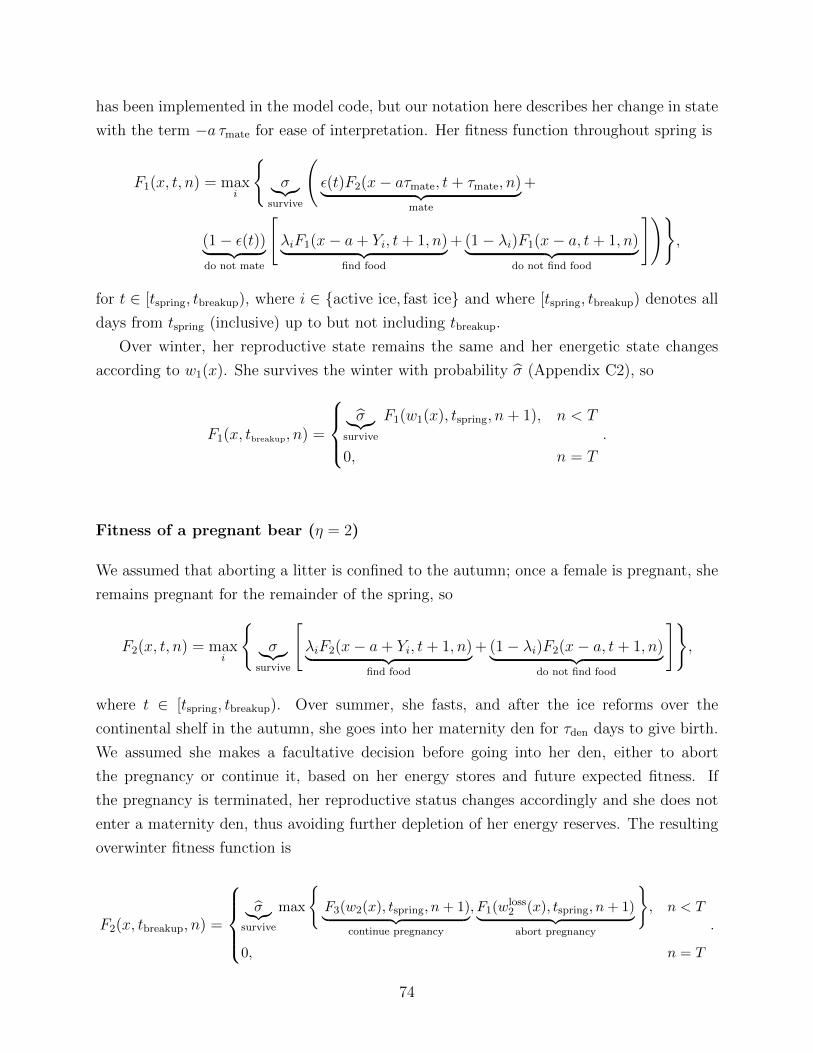
has been implemented in the model code, but our notation here describes her change in state

with the term −a τmate for ease of interpretation. Her fitness function throughout spring is

F1(x, t, n) = maxi

{σ⏞⏟⏟⏞

survive

(ϵ(t)F2(x− aτmate, t+ τmate, n)⏞ ⏟⏟ ⏞

mate

+

(1− ϵ(t))⏞ ⏟⏟ ⏞do not mate

[λiF1(x− a+ Yi, t+ 1, n)⏞ ⏟⏟ ⏞

find food

+(1− λi)F1(x− a, t+ 1, n)⏞ ⏟⏟ ⏞do not find food

])},

for t ∈ [tspring, tbreakup), where i ∈ {active ice, fast ice} and where [tspring, tbreakup) denotes all

days from tspring (inclusive) up to but not including tbreakup.

Over winter, her reproductive state remains the same and her energetic state changes

according to w1(x). She survives the winter with probability ˆσ (Appendix C2), so

F1(x, tbreakup, n) =

⎧⎪⎨⎪⎩ˆσ⏞⏟⏟⏞

survive

F1(w1(x), tspring, n+ 1), n < T

0, n = T

.

Fitness of a pregnant bear (η = 2)

We assumed that aborting a litter is confined to the autumn; once a female is pregnant, she

remains pregnant for the remainder of the spring, so

F2(x, t, n) = maxi

{σ⏞⏟⏟⏞

survive

[λiF2(x− a+ Yi, t+ 1, n)⏞ ⏟⏟ ⏞

find food

+(1− λi)F2(x− a, t+ 1, n)⏞ ⏟⏟ ⏞do not find food

]},

where t ∈ [tspring, tbreakup). Over summer, she fasts, and after the ice reforms over the

continental shelf in the autumn, she goes into her maternity den for τden days to give birth.

We assumed she makes a facultative decision before going into her den, either to abort

the pregnancy or continue it, based on her energy stores and future expected fitness. If

the pregnancy is terminated, her reproductive status changes accordingly and she does not

enter a maternity den, thus avoiding further depletion of her energy reserves. The resulting

overwinter fitness function is

F2(x, tbreakup, n) =

⎧⎪⎪⎨⎪⎪⎩ˆσ⏞⏟⏟⏞

survive

max

{F3(w2(x), tspring, n+ 1)⏞ ⏟⏟ ⏞

continue pregnancy

, F1(wloss2 (x), tspring, n+ 1)⏞ ⏟⏟ ⏞abort pregnancy

}, n < T

0, n = T

.

74

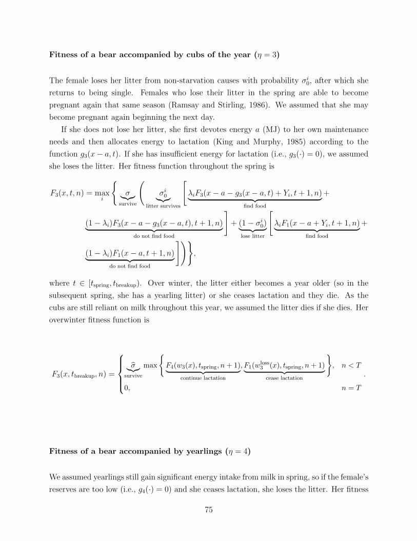
Fitness of a bear accompanied by cubs of the year (η = 3)

The female loses her litter from non-starvation causes with probability σi0, after which she

returns to being single. Females who lose their litter in the spring are able to become

pregnant again that same season (Ramsay and Stirling, 1986). We assumed that she may

become pregnant again beginning the next day.

If she does not lose her litter, she first devotes energy a (MJ) to her own maintenance

needs and then allocates energy to lactation (King and Murphy, 1985) according to the

function g3(x− a, t). If she has insufficient energy for lactation (i.e., g3(·) = 0), we assumed

she loses the litter. Her fitness function throughout the spring is

F3(x, t, n) = maxi

{σ⏞⏟⏟⏞

survive

(σi0⏞⏟⏟⏞

litter survives

[λiF3(x− a− g3(x− a, t) + Yi, t+ 1, n)⏞ ⏟⏟ ⏞

find food

+

(1− λi)F3(x− a− g3(x− a, t), t+ 1, n)⏞ ⏟⏟ ⏞do not find food

]+ (1− σi

0)⏞ ⏟⏟ ⏞lose litter

[λiF1(x− a+ Yi, t+ 1, n)⏞ ⏟⏟ ⏞

find food

+

(1− λi)F1(x− a, t+ 1, n)⏞ ⏟⏟ ⏞do not find food

])},

where t ∈ [tspring, tbreakup). Over winter, the litter either becomes a year older (so in the

subsequent spring, she has a yearling litter) or she ceases lactation and they die. As the

cubs are still reliant on milk throughout this year, we assumed the litter dies if she dies. Her

overwinter fitness function is

F3(x, tbreakup, n) =

⎧⎪⎪⎨⎪⎪⎩ˆσ⏞⏟⏟⏞

survive

max

{F4(w3(x), tspring, n+ 1)⏞ ⏟⏟ ⏞

continue lactation

, F1(wloss3 (x), tspring, n+ 1)⏞ ⏟⏟ ⏞

cease lactation

}, n < T

0, n = T

.

Fitness of a bear accompanied by yearlings (η = 4)

We assumed yearlings still gain significant energy intake from milk in spring, so if the female’s

reserves are too low (i.e., g4(·) = 0) and she ceases lactation, she loses the litter. Her fitness

75

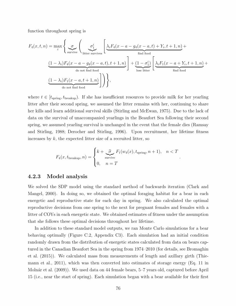
function throughout spring is

F4(x, t, n) = maxi

{σ⏞⏟⏟⏞

survive

(σi1⏞⏟⏟⏞

litter survives

[λiF4(x− a− g4(x− a, t) + Yi, t+ 1, n)⏞ ⏟⏟ ⏞

find food

+

(1− λi)F4(x− a− g4(x− a, t), t+ 1, n)⏞ ⏟⏟ ⏞do not find food

]+ (1− σi

1)⏞ ⏟⏟ ⏞lose litter

[λiF1(x− a+ Yi, t+ 1, n)⏞ ⏟⏟ ⏞

find food

+

(1− λi)F1(x− a, t+ 1, n)⏞ ⏟⏟ ⏞do not find food

])},

where t ∈ [tspring, tbreakup). If she has insufficient resources to provide milk for her yearling

litter after their second spring, we assumed the litter remains with her, continuing to share

her kills and learn additional survival skills (Stirling and McEwan, 1975). Due to the lack of

data on the survival of unaccompanied yearlings in the Beaufort Sea following their second

spring, we assumed yearling survival is unchanged in the event that the female dies (Ramsay

and Stirling, 1988; Derocher and Stirling, 1996). Upon recruitment, her lifetime fitness

increases by k, the expected litter size of a recruited litter, so

F4(x, tbreakup, n) =

⎧⎪⎨⎪⎩k + ˆσ⏞⏟⏟⏞

survive

F1(w4(x), tspring, n+ 1), n < T

0, n = T

.

4.2.3 Model analysis

We solved the SDP model using the standard method of backwards iteration (Clark and

Mangel, 2000). In doing so, we obtained the optimal foraging habitat for a bear in each

energetic and reproductive state for each day in spring. We also calculated the optimal

reproductive decisions from one spring to the next for pregnant females and females with a

litter of COYs in each energetic state. We obtained estimates of fitness under the assumption

that she follows these optimal decisions throughout her lifetime.

In addition to these standard model outputs, we ran Monte Carlo simulations for a bear

behaving optimally (Figure C.2, Appendix C3). Each simulation had an initial condition

randomly drawn from the distribution of energetic states calculated from data on bears cap-

tured in the Canadian Beaufort Sea in the spring from 1974–2010 (for details, see Bromaghin

et al. (2015)). We calculated mass from measurements of length and axillary girth (Thie-

mann et al., 2011), which was then converted into estimates of storage energy (Eq. 11 in

Molnar et al. (2009)). We used data on 44 female bears, 5–7 years old, captured before April

15 (i.e., near the start of spring). Each simulation began with a bear available for their first

76

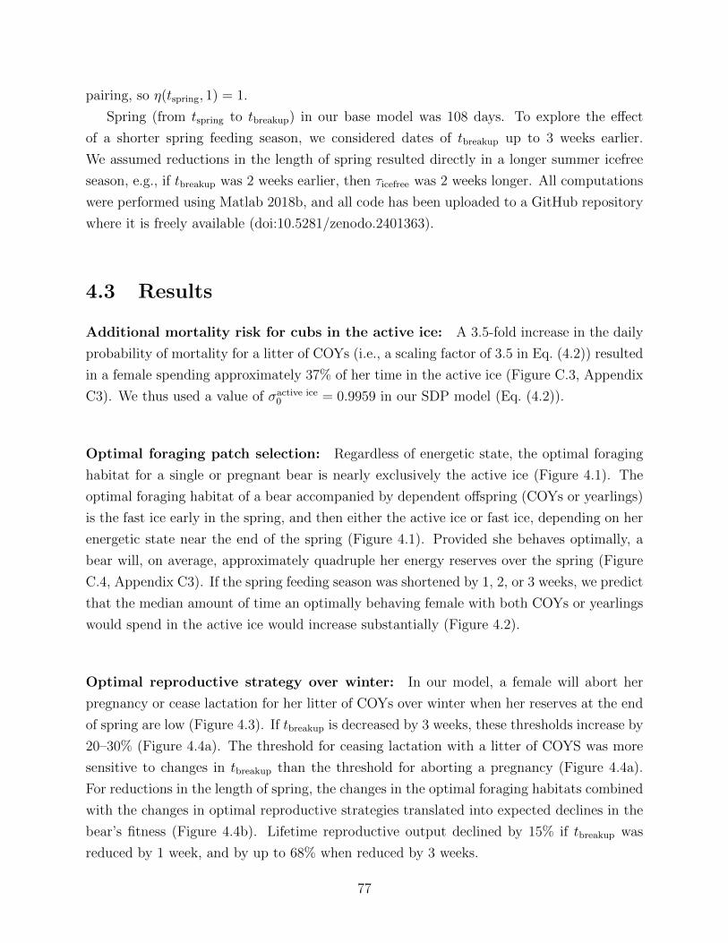
pairing, so η(tspring, 1) = 1.

Spring (from tspring to tbreakup) in our base model was 108 days. To explore the effect

of a shorter spring feeding season, we considered dates of tbreakup up to 3 weeks earlier.

We assumed reductions in the length of spring resulted directly in a longer summer icefree

season, e.g., if tbreakup was 2 weeks earlier, then τicefree was 2 weeks longer. All computations

were performed using Matlab 2018b, and all code has been uploaded to a GitHub repository

where it is freely available (doi:10.5281/zenodo.2401363).

4.3 Results

Additional mortality risk for cubs in the active ice: A 3.5-fold increase in the daily

probability of mortality for a litter of COYs (i.e., a scaling factor of 3.5 in Eq. (4.2)) resulted

in a female spending approximately 37% of her time in the active ice (Figure C.3, Appendix

C3). We thus used a value of σactive ice0 = 0.9959 in our SDP model (Eq. (4.2)).

Optimal foraging patch selection: Regardless of energetic state, the optimal foraging

habitat for a single or pregnant bear is nearly exclusively the active ice (Figure 4.1). The

optimal foraging habitat of a bear accompanied by dependent offspring (COYs or yearlings)

is the fast ice early in the spring, and then either the active ice or fast ice, depending on her

energetic state near the end of the spring (Figure 4.1). Provided she behaves optimally, a

bear will, on average, approximately quadruple her energy reserves over the spring (Figure

C.4, Appendix C3). If the spring feeding season was shortened by 1, 2, or 3 weeks, we predict

that the median amount of time an optimally behaving female with both COYs or yearlings

would spend in the active ice would increase substantially (Figure 4.2).

Optimal reproductive strategy over winter: In our model, a female will abort her

pregnancy or cease lactation for her litter of COYs over winter when her reserves at the end

of spring are low (Figure 4.3). If tbreakup is decreased by 3 weeks, these thresholds increase by

20–30% (Figure 4.4a). The threshold for ceasing lactation with a litter of COYS was more

sensitive to changes in tbreakup than the threshold for aborting a pregnancy (Figure 4.4a).

For reductions in the length of spring, the changes in the optimal foraging habitats combined

with the changes in optimal reproductive strategies translated into expected declines in the

bear’s fitness (Figure 4.4b). Lifetime reproductive output declined by 15% if tbreakup was

reduced by 1 week, and by up to 68% when reduced by 3 weeks.

77

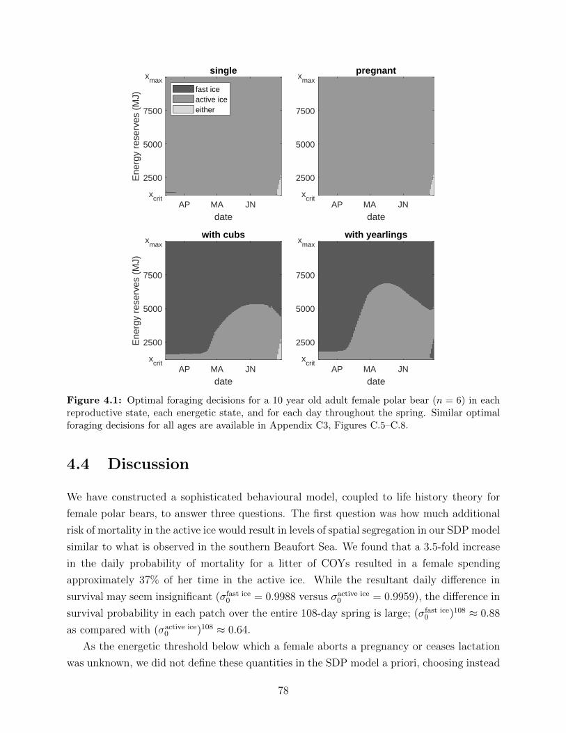
single

AP MA JN

date

xmax

7500

5000

2500

xcrit

Ene

rgy

rese

rves

(M

J)

fast iceactive iceeither

pregnant

AP MA JN

date

xmax

7500

5000

2500

xcrit

with cubs

AP MA JN

date

xmax

7500

5000

2500

xcrit

Ene

rgy

rese

rves

(M

J)

with yearlings

AP MA JN

date

xmax

7500

5000

2500

xcrit

Figure 4.1: Optimal foraging decisions for a 10 year old adult female polar bear (n = 6) in eachreproductive state, each energetic state, and for each day throughout the spring. Similar optimalforaging decisions for all ages are available in Appendix C3, Figures C.5–C.8.

4.4 Discussion

We have constructed a sophisticated behavioural model, coupled to life history theory for

female polar bears, to answer three questions. The first question was how much additional

risk of mortality in the active ice would result in levels of spatial segregation in our SDP model

similar to what is observed in the southern Beaufort Sea. We found that a 3.5-fold increase

in the daily probability of mortality for a litter of COYs resulted in a female spending

approximately 37% of her time in the active ice. While the resultant daily difference in

survival may seem insignificant (σfast ice0 = 0.9988 versus σactive ice

0 = 0.9959), the difference in

survival probability in each patch over the entire 108-day spring is large; (σfast ice0 )108 ≈ 0.88

as compared with (σactive ice0 )108 ≈ 0.64.

As the energetic threshold below which a female aborts a pregnancy or ceases lactation

was unknown, we did not define these quantities in the SDP model a priori, choosing instead

78

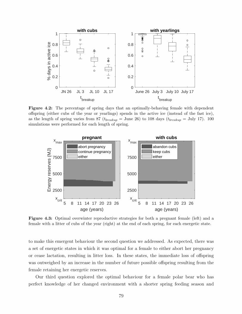
JN 26 JL 3 JL 10 JL 17

tbreakup

0

0.2

0.4

0.6

0.8

1

% d

ays

in a

ctiv

e ic

e

with cubs

June 26 July 3 July 10 July 17

tbreakup

0

0.2

0.4

0.6

0.8

1with yearlings

Figure 4.2: The percentage of spring days that an optimally-behaving female with dependentoffspring (either cubs of the year or yearlings) spends in the active ice (instead of the fast ice),as the length of spring varies from 87 (tbreakup = June 26) to 108 days (tbreakup = July 17). 100simulations were performed for each length of spring.

pregnant

5 8 11 14 17 20 23 26

age (years)

xmax

7500

5000

2500

xcrit

Ene

rgy

rese

rves

(M

J)

abort pregnancycontinue pregnancyeither

with cubs

5 8 11 14 17 20 23 26

age (years)

xmax

7500

5000

2500

xcrit

abandon cubskeep cubseither

Figure 4.3: Optimal overwinter reproductive strategies for both a pregnant female (left) and afemale with a litter of cubs of the year (right) at the end of each spring, for each energetic state.

to make this emergent behaviour the second question we addressed. As expected, there was

a set of energetic states in which it was optimal for a female to either abort her pregnancy

or cease lactation, resulting in litter loss. In these states, the immediate loss of offspring

was outweighed by an increase in the number of future possible offspring resulting from the

female retaining her energetic reserves.

Our third question explored the optimal behaviour for a female polar bear who has

perfect knowledge of her changed environment with a shorter spring feeding season and

79

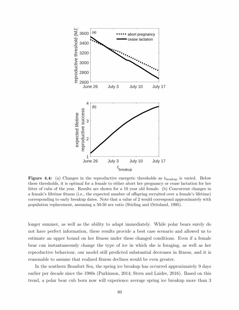
June 26 July 3 July 10 July 172600

2800

3000

3200

3400

3600

repr

oduc

tive

thre

shol

d (M

J)

(a)abort pregnancycease lactation

June 26 July 3 July 10 July 17

tbreakup

1

2

3

4

expe

cted

life

time

repr

oduc

tive

succ

ess (b)

Figure 4.4: (a) Changes in the reproductive energetic thresholds as tbreakup is varied. Belowthese thresholds, it is optimal for a female to either abort her pregnancy or cease lactation for herlitter of cubs of the year. Results are shown for a 10 year old female. (b) Concurrent changes ina female’s lifetime fitness (i.e., the expected number of offspring recruited over a female’s lifetime)corresponding to early breakup dates. Note that a value of 2 would correspond approximately withpopulation replacement, assuming a 50:50 sex ratio (Stirling and Øritsland, 1995).

longer summer, as well as the ability to adapt immediately. While polar bears surely do

not have perfect information, these results provide a best case scenario and allowed us to

estimate an upper bound on her fitness under these changed conditions. Even if a female

bear can instantaneously change the type of ice in which she is foraging, as well as her

reproductive behaviour, our model still predicted substantial decreases in fitness, and it is

reasonable to assume that realized fitness declines would be even greater.

In the southern Beaufort Sea, the spring ice breakup has occurred approximately 9 days

earlier per decade since the 1980s (Parkinson, 2014; Stern and Laidre, 2016). Based on this

trend, a polar bear cub born now will experience average spring ice breakup more than 3

80

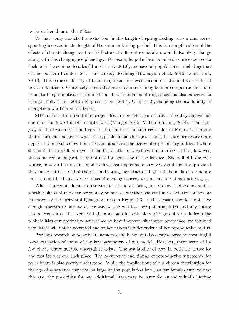
weeks earlier than in the 1980s.

We have only modelled a reduction in the length of spring feeding season and corre-

sponding increase in the length of the summer fasting period. This is a simplification of the

effects of climate change, as the risk factors of different ice habitats would also likely change

along with this changing ice phenology. For example, polar bear populations are expected to

decline in the coming decades (Hunter et al., 2010), and several populations – including that

of the southern Beaufort Sea – are already declining (Bromaghin et al., 2015; Lunn et al.,

2016). This reduced density of bears may result in lower encounter rates and so a reduced

risk of infanticide. Conversely, bears that are encountered may be more desperate and more

prone to hunger-motivated cannibalism. The abundance of ringed seals is also expected to

change (Kelly et al. (2010); Ferguson et al. (2017), Chapter 2), changing the availability of

energetic rewards in all ice types.

SDP models often result in emergent features which seem intuitive once they appear but

one may not have thought of otherwise (Mangel, 2015; McHuron et al., 2018). The light

gray in the lower right hand corner of all but the bottom right plot in Figure 4.1 implies

that it does not matter in which ice type the female forages. This is because her reserves are

depleted to a level so low that she cannot survive the overwinter period, regardless of where

she hunts in those final days. If she has a litter of yearlings (bottom right plot), however,

this same region suggests it is optimal for her to be in the fast ice. She will still die over

winter, however because our model allows yearling cubs to survive even if she dies, provided

they make it to the end of their second spring, her fitness is higher if she makes a desperate

final attempt in the active ice to acquire enough energy to continue lactating until tbreakup.

When a pregnant female’s reserves at the end of spring are too low, it does not matter

whether she continues her pregnancy or not, or whether she continues lactation or not, as

indicated by the horizontal light gray areas in Figure 4.3. In these cases, she does not have

enough reserves to survive either way so she will lose her potential litter and any future

litters, regardless. The vertical light gray bars in both plots of Figure 4.3 result from the

probabilities of reproductive senescence we have imposed, since after senescence, we assumed

new litters will not be recruited and so her fitness is independent of her reproductive status.

Previous research on polar bear energetics and behavioural ecology allowed for meaningful

parametrization of many of the key parameters of our model. However, there were still a

few places where notable uncertainty exists. The availability of prey in both the active ice

and fast ice was one such place. The occurrence and timing of reproductive senescence for

polar bears is also poorly understood. While the implications of our chosen distribution for

the age of senescence may not be large at the population level, as few females survive past

this age, the possibility for one additional litter may be large for an individual’s lifetime

81

reproductive success. Reproductive senescence in female polar bears is thought to effectively

result from a decline in body condition with age (Derocher and Stirling, 1994). However, as

we have not included this level of detail in our model (i.e., including a change in female’s

hunting ability and knowledge over time), we have imposed senescence in this way.

Our work leads to several new predictions, for which the data are already available to

explore. Data on polar bear body condition, as well as the location, date, and reproductive

status of each bear were collected for population monitoring. The results of our model suggest

exploring if females with cubs in poor body condition are more often found in the active

ice than females in better condition. Further, our results suggest that a female with cubs

may spend more time in the active ice as breakup occurs earlier. A shift of female hunting

habitat choice may already be apparent over the past several decades as the breakup day

has gotten earlier (Parkinson, 2014; Stern and Laidre, 2016).

SDP models allow us to explore both what types of selective forces may have led to

observed traits as well as explore bounds for how individuals may adapt to new conditions.

Models such as this one allow us to consider interactions between several important concepts,

including changing ecological conditions, behavioural plasticity, reproductive biology and

optimal foraging. This can lead to new predictions, as well as sharpening our intuition

about the tradeoffs faced by individuals in complex ecological landscapes.

Appendices

C1 Parametrization and functional forms

We parametrized our model and chose functional forms to reflect the ecology of the southern

Beaufort Sea population of polar bears.

Energetic state constraints

xcrit

We assumed that if a bear’s energy reserves are reduced to xcrit = 0 MJ, the bear dies of

starvation (Molnar et al., 2009).

xmax

We assumed a maximum mass of four times a bear’s structural mass (Molnar et al., 2009).

Structural mass was calculated as in Eq. (4.3), with x(t) = 0. The storage energy of a

82

bear with this maximum mass was estimated using equations (11) and (12) in Molnar et al.

(2009). For a bear of length L= 1.96m, xmax = 8822 MJ.

Time parameters

T

We assumed a female is first available to mate in the spring at age 5. As females generally

stop reproducing in their late 20s, we have taken a maximum age of 28, since she will not

have any fitness gains after this age. Thus the number of years we consider is T = 24.

tspring

Ringed seal pupping begins in early April, reaching its peak mid-April (McLaren, 1958;

Smith, 1987), so we assumed polar bears may start experiencing net energetic gains at

approximately tspring = April 1 (ordinal day 91).

tbreakup

We assumed net energetic gains decline sharply around the time of sea ice breakup, defined

as the first day on which the average sea ice concentration over the Southern Beaufort Sea

subpopulation area declined below 50% (Etkin, 1991; Stirling, 2005; Ferguson et al., 2017).

Sea ice data was obtained from the National Snow and Ice Data Center (Stroeve and Meier,

2018). Satellite imagery was available from 1979 until the present, but in an attempt to

capture the scenario before significant climate change impacts, we calculated the average

breakup date using only the 1980s, resulting in tbreakup = July 17 (ordinal day 198).

τicefree

As above, we calculated freezeup as the first day in autumn that the mean sea ice concen-

tration rose above 50%. The mean day of freezeup in the 1980s was tfreezeup = October 8

(ordinal day 281). The number of days between breakup and freezeup was τicefree = 83.

General parameters

λi

The daily probability of finding and catching prey is thought to depend on patch choice

between active ice and fast ice, with active ice believed to have a higher density of prey

that are more vulnerable to predation. Stirling and Øritsland (1995) estimated that bears

83

caught a seal approximately every 3 days in the spring. We used λfast ice = 1/3.5 and

λactive ice = 1/2.5.

Yi(t)

When a polar bear catches a prey item, the expected energetic value depends on the type

and size of seals available in patch i at time t. The expected value of prey for a given ice

habitat (i = fast ice or active ice) was calculated as

Yi(t) =∑

species

[Pr(species)

( ∑seal class

Pr(seal class|species)× (energetic value|seal class, species)

)],

where ‘species’ ranged through ringed and bearded seals and ‘seal class’ ranged through pups

and juveniles/adults. Each of the probabilities was conditional on patch, i, and date, t. The

Pr(species) depended on habitat. Estimates were made using data on seals killed by polar

bears in the Beaufort Sea (data from Pilfold et al. (2012)). In the fast ice, where bearded

seals are uncommon, Pr(ringed seals) = 0.97 and Pr(bearded seals) = 0.03. In the active

ice, these values changed to be 0.84 and 0.16, respectively.

The Pr(seal class|species) also depended on habitat. In the fast ice, pups made up 52%

of the observed ringed seal kills, while juveniles/adults made up 48%. In the active ice,

ringed seal pup kills were observed with higher frequency, and these values changed to 72%

and 28%, respectively. Of the few bearded seal kills observed, all were juveniles/adults in

the fast ice, while 27% were pups and 73% were adults in the active ice.

We used previous estimates for the energetic values of ringed seals. Gross energy estimates

for ringed seal pups were 41.9 MJ through April, 209.3 from May 1–15, and 418.7 MJs for the

remainder of the spring (Stirling and Øritsland, 1995). Subadult and adult ringed seals have

a gross energy content of approximately 628 MJs (Stirling and Øritsland, 1995). However, a

polar bear is thought to only be able to eat a maximum 20% of its mass in one meal (Best,

1977). Thus for a female polar bear who may average 200kg, we assumed she may consume

a maximum of 40kg per day. An adult ringed seal weighs an average of 57 kg (Lydersen and

Gjertz, 1987). If the female can only eat 40 kg, she consumes approximately 70% (= 40/57)

of the available mass. We thus assumed maximum energetic intake in one day to be 439.6

MJs (= 0.7 ∗ 628).In the absence of information on the energetic value of bearded seal pups, we multiplied

the ringed seal pup energetic values by a scaling factor to obtain estimates for the calories

obtained from bearded seal pups. To obtain this scaling factor, we divided the average mass

of bearded seal pups (62kg (Derocher et al., 2002)) by the average mass of ringed seals pups

84

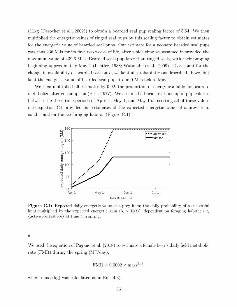
(11kg (Derocher et al., 2002)) to obtain a bearded seal pup scaling factor of 5.64. We then

multiplied the energetic values of ringed seal pups by this scaling factor to obtain estimates

for the energetic value of bearded seal pups. Our estimate for a neonate bearded seal pups

was thus 236 MJs for its first two weeks of life, after which time we assumed it provided the

maximum value of 439.6 MJs. Bearded seals pup later than ringed seals, with their pupping

beginning approximately May 1 (Lentfer, 1988; Watanabe et al., 2009). To account for the

change in availability of bearded seal pups, we kept all probabilities as described above, but

kept the energetic value of bearded seal pups to be 0 MJs before May 1.

We then multiplied all estimates by 0.92, the proportion of energy available for bears to

metabolize after consumption (Best, 1977). We assumed a linear relationship of pup calories

between the three time periods of April 1, May 1, and May 15. Inserting all of these values

into equation C1 provided our estimates of the expected energetic value of a prey item,

conditional on the ice foraging habitat (Figure C.1).

Apr 1 May 1 Jun 1 Jul 1

day in spring 2000

60

80

100

120

140

160

expe

cted

dai

ly e

nerg

etic

gai

n (M

J)

active icefast ice

Figure C.1: Expected daily energetic value of a prey item; the daily probability of a successfulhunt multiplied by the expected energetic gain (λi × Yi(t)), dependent on foraging habitat i ∈{active ice, fast ice} at time t in spring.

a

We used the equation of Pagano et al. (2018) to estimate a female bear’s daily field metabolic

rate (FMR) during the spring (MJ/day),

FMR = 0.0002×mass2.41,

where mass (kg) was calculated as in Eq. (4.3).

85

σ

We used 0.996 as our estimate of an adult female bear’s annual survival probability in

the Beaufort Sea (Amstrup and Durner, 1995). We assumed daily survival to be constant

throughout the year, so daily survival was calculated as the 365th root of annual survival,

σ = 0.996365−1

.

ˆσThe number of days not considered as part of spring was

# of ‘overwinter’ days = 365− (tbreakup − tspring),

which, for our estimated parameter values, was 258 days. The probability of overwinter

survival ˆσ was calculated from the daily survival probabilities, multiplied by the number

of days included in the ‘overwinter’ period, so ˆσ = σ258 ≈ 0.9972. Note that we updated

this value each time we considered an earlier breakup and corresponding longer ‘overwinter’

period.

ps(age)

Functional reproductive senescence has been suggested to occur during a female’s early 20s

(Ramsay and Stirling, 1988; Derocher and Stirling, 1994; Regehr et al., 2007; Stirling et al.,

2011). While polar bears are physiologically able to reproduce into their 30s in captivity

(Latinen, 1987), they may have trouble accumulating sufficient fat stores to do so in the wild

after their prime years (Derocher and Stirling, 1994).

We used the generalized extreme value distribution to describe the probability of senes-

cence occurring at a given age, as was used to successfully model grizzly bear (Ursus arctos)

senescence (Schwartz et al., 2003). We used a value of 1 for the shape parameter, as found

for grizzly bears (Schwartz et al., 2003), but shifted the distribution to have a mode at age

23, resulting in the probability density function

f(x) = e−(x/23)23( x23

)22,

where x is the bear’s age, to the day, converted into decimal years. To get the probability

86

of senescence over an entire year, we integrated, so

ps(age) =

∫ age+1

age

e−(x/23)23( x23

)22dx.

As we assumed a bear must become senescent, we use a conditional probability to capture

the probability of becoming senescent at a given age, given that she is not yet senescent by

her current age, i.e.,

ps(age) =

∫ age+1

agee−(x/23)23

(x23

)22dx∫∞

agee−(x/23)23

(x23

)22dx

.

This resulted in a left-skewed probability density function, where the probability of becoming

senescent between ages 20 and 25 is 0.96 (specifically, the probabilities of becoming senescent

before age 20 or after age 25 are 0.039 and 0.001, respectively).

Single (η = 1) parameters

ϵ(t)

The probability of a single bear mating is high, here taken to be 0.99 over the entire spring

(Molnar et al., 2008). We assumed that the daily probability of finding a mate is independent

of age, and does not vary over the mating season. Mating must start τmate days before

breakup, in order for there to be sufficient time for the pair to mate successfully, so the

number of days where a female is available to mate is

mating days = (tbreakup − τmate)− tspring.

This resulted in the daily probability of finding a mate,

ϵ(t) = 1− probability of not finding a mate

= 1− (1− 0.99)1/(mating days)

for t = 1, . . . , (mating days). For our values of tspring, tbreakup, and τmate, this resulted in a

daily estimate of ϵ(t) ≈ 0.05. If the depletion of the female’s reserves following mating would

cause her to die, we assumed she does not mate.

τmate

Mating takes approximately 17 days (Molnar et al., 2008), with other estimates around this

value: 16 days (Derocher et al., 2010), 18 days (Wiig et al., 1992), and 13 days (Stirling

87

et al., 2016).

Pregnancy (η = 2) parameters

τden

We assumed den entry and emergence occur approximately on November 17 and March 31,

respectively (Amstrup and Gardner, 1994), so τden = 134.

Cubs of the year litter (η = 3) parameters

σfast ice0

Using the annual survival probability of 0.651 of a COY litter from Amstrup and Durner

(1995), we took the daily probability of survival to be the 365th root of this value. We

assumed this value pertains to females with COYs who spend their time mainly in the fast

ice, so σfast ice0 = 0.651365

−1.

g3(x, t), g4(x, t)

For a female with a litter of dependent COYs or yearlings (η = 3, 4), the female has some

energetic threshold below which lactation ceases (Robbins et al., 2012). However, female

bears likely do not approach this threshold in the spring when food is abundant, and so for

this part of our model, we assumed this threshold to be xcrit, i.e., the female will not produce

milk if it causes her to die, but otherwise she will. While this is a simplification, we do not

expect it affect our results in a meaningful way.

If the female is well above xcrit, she invests a target amount, mη, daily, and if she is unable

to invest mη without falling to xcrit, she ceases lactation. The energetic costs of lactation

were,

gη(x(t)) =

⎧⎨⎩mη, x > xcrit +mη

0, else, η = 3, 4.

The litter is lost if a female’s reserves are too low to produce milk (i.e., gη(x(t)) = 0).

We assumed m3 = 0.24 ×mass0.75, the milk production of black bears (Ursus americanus)

during mid-lactation (Gittleman and Oftedal, 1987; Arnould and Ramsay, 1994), and m4 =

0.1 × mass0.75, as it falls between the values of 0.17 and 0.05 ×mass0.75 describing milk

production over a litter’s first and second summers, respectively (Arnould and Ramsay,

1994).

88

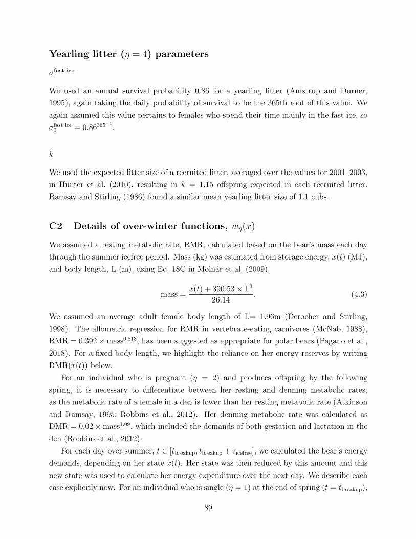
Yearling litter (η = 4) parameters

σfast ice1

We used an annual survival probability 0.86 for a yearling litter (Amstrup and Durner,

1995), again taking the daily probability of survival to be the 365th root of this value. We

again assumed this value pertains to females who spend their time mainly in the fast ice, so

σfast ice0 = 0.86365

−1.

k

We used the expected litter size of a recruited litter, averaged over the values for 2001–2003,

in Hunter et al. (2010), resulting in k = 1.15 offspring expected in each recruited litter.

Ramsay and Stirling (1986) found a similar mean yearling litter size of 1.1 cubs.

C2 Details of over-winter functions, wη(x)

We assumed a resting metabolic rate, RMR, calculated based on the bear’s mass each day

through the summer icefree period. Mass (kg) was estimated from storage energy, x(t) (MJ),

and body length, L (m), using Eq. 18C in Molnar et al. (2009).

mass =x(t) + 390.53× L3

26.14. (4.3)

We assumed an average adult female body length of L= 1.96m (Derocher and Stirling,

1998). The allometric regression for RMR in vertebrate-eating carnivores (McNab, 1988),

RMR = 0.392×mass0.813, has been suggested as appropriate for polar bears (Pagano et al.,

2018). For a fixed body length, we highlight the reliance on her energy reserves by writing

RMR(x(t)) below.

For an individual who is pregnant (η = 2) and produces offspring by the following

spring, it is necessary to differentiate between her resting and denning metabolic rates,

as the metabolic rate of a female in a den is lower than her resting metabolic rate (Atkinson

and Ramsay, 1995; Robbins et al., 2012). Her denning metabolic rate was calculated as

DMR = 0.02×mass1.09, which included the demands of both gestation and lactation in the

den (Robbins et al., 2012).

For each day over summer, t ∈ [tbreakup, tbreakup + τicefree], we calculated the bear’s energy

demands, depending on her state x(t). Her state was then reduced by this amount and this

new state was used to calculate her energy expenditure over the next day. We describe each

case explicitly now. For an individual who is single (η = 1) at the end of spring (t = tbreakup),

89

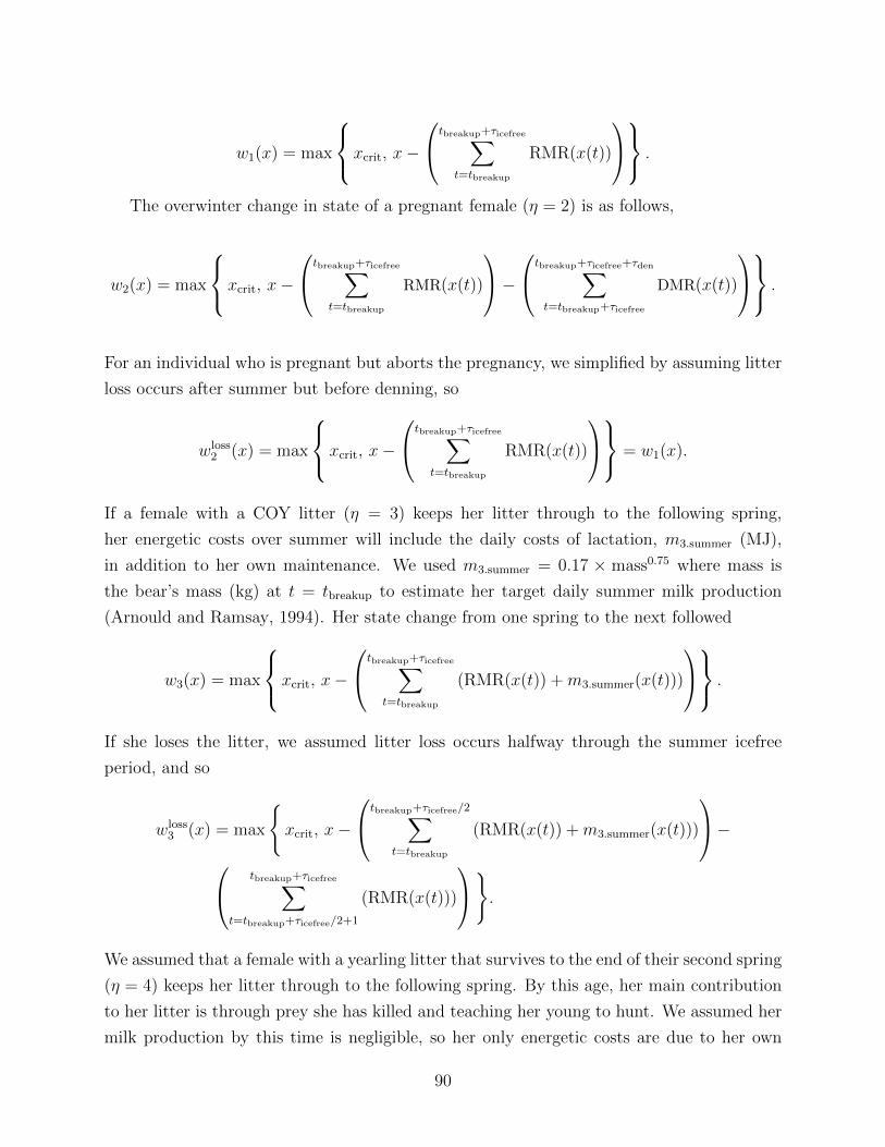
w1(x) = max

⎧⎨⎩xcrit, x−

⎛⎝tbreakup+τicefree∑t=tbreakup

RMR(x(t))

⎞⎠⎫⎬⎭ .

The overwinter change in state of a pregnant female (η = 2) is as follows,

w2(x) = max

⎧⎨⎩xcrit, x−

⎛⎝tbreakup+τicefree∑t=tbreakup

RMR(x(t))

⎞⎠−

⎛⎝tbreakup+τicefree+τden∑t=tbreakup+τicefree

DMR(x(t))

⎞⎠⎫⎬⎭ .

For an individual who is pregnant but aborts the pregnancy, we simplified by assuming litter

loss occurs after summer but before denning, so

wloss2 (x) = max

⎧⎨⎩xcrit, x−

⎛⎝tbreakup+τicefree∑t=tbreakup

RMR(x(t))

⎞⎠⎫⎬⎭ = w1(x).

If a female with a COY litter (η = 3) keeps her litter through to the following spring,

her energetic costs over summer will include the daily costs of lactation, m3.summer (MJ),

in addition to her own maintenance. We used m3.summer = 0.17 × mass0.75 where mass is

the bear’s mass (kg) at t = tbreakup to estimate her target daily summer milk production

(Arnould and Ramsay, 1994). Her state change from one spring to the next followed

w3(x) = max

⎧⎨⎩xcrit, x−

⎛⎝tbreakup+τicefree∑t=tbreakup

(RMR(x(t)) +m3.summer(x(t)))

⎞⎠⎫⎬⎭ .

If she loses the litter, we assumed litter loss occurs halfway through the summer icefree

period, and so

wloss3 (x) = max

{xcrit, x−

⎛⎝tbreakup+τicefree/2∑t=tbreakup

(RMR(x(t)) +m3.summer(x(t)))

⎞⎠−

⎛⎝ tbreakup+τicefree∑t=tbreakup+τicefree/2+1

(RMR(x(t)))

⎞⎠}.We assumed that a female with a yearling litter that survives to the end of their second spring

(η = 4) keeps her litter through to the following spring. By this age, her main contribution

to her litter is through prey she has killed and teaching her young to hunt. We assumed her

milk production by this time is negligible, so her only energetic costs are due to her own

90

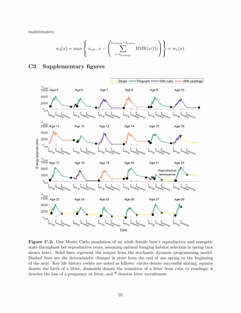
maintenance,

w4(x) = max

⎧⎨⎩xcrit, x−

⎛⎝tbreakup+τicefree∑t=tbreakup

RMR(x(t))

⎞⎠⎫⎬⎭ = w1(x).

C3 Supplementary figures

Figure C.2: One Monte Carlo simulation of an adult female bear’s reproductive and energeticstate throughout her reproductive years, assuming optimal foraging habitat selection in spring (notshown here). Solid lines represent the output from the stochastic dynamic programming model.Dashed lines are the deterministic changes in state from the end of one spring to the beginningof the next. Key life history events are noted as follows: circles denote successful mating; squaresdenote the birth of a litter; diamonds denote the transition of a litter from cubs to yearlings; xdenotes the loss of a pregnancy or litter; and * denotes litter recruitment.

91

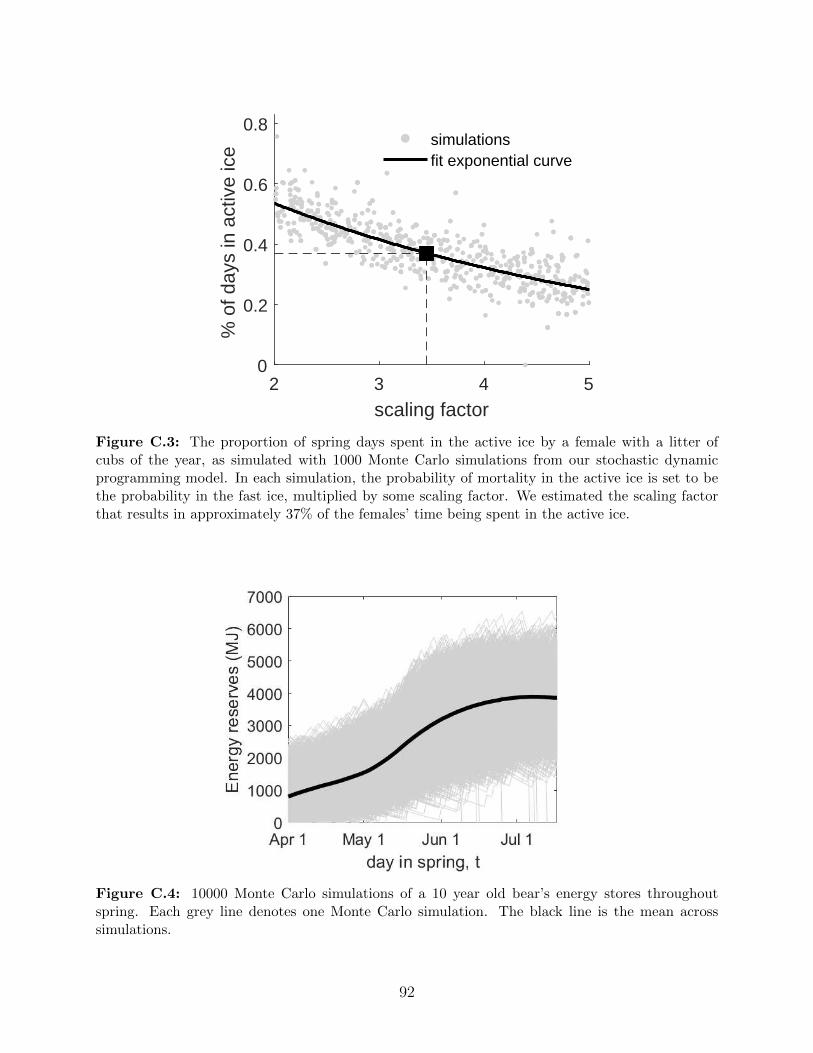
2 3 4 5

scaling factor

0

0.2

0.4

0.6

0.8

% o

f day

s in

act

ive

ice

simulationsfit exponential curve

Figure C.3: The proportion of spring days spent in the active ice by a female with a litter ofcubs of the year, as simulated with 1000 Monte Carlo simulations from our stochastic dynamicprogramming model. In each simulation, the probability of mortality in the active ice is set to bethe probability in the fast ice, multiplied by some scaling factor. We estimated the scaling factorthat results in approximately 37% of the females’ time being spent in the active ice.

Figure C.4: 10000 Monte Carlo simulations of a 10 year old bear’s energy stores throughoutspring. Each grey line denotes one Monte Carlo simulation. The black line is the mean acrosssimulations.

92

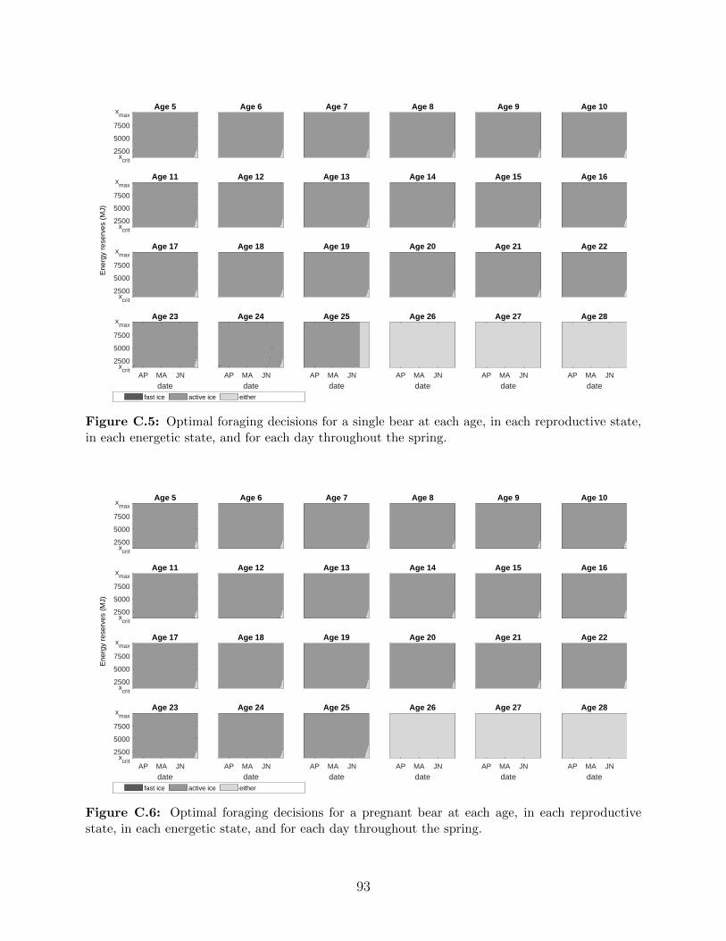
Age 5xmax

7500

5000

2500xcrit

fast ice active ice either

Age 6 Age 7 Age 8 Age 9 Age 10

Age 11

Ene

rgy

rese

rves

(M

J)

xmax

7500

5000

2500xcrit

Age 12 Age 13 Age 14 Age 15 Age 16

Age 17xmax

7500

5000

2500xcrit

Age 18 Age 19 Age 20 Age 21 Age 22

Age 23

AP MA JN

date

xmax

7500

5000

2500xcrit

Age 24

AP MA JN

date

Age 25

AP MA JN

date

Age 26

AP MA JN

date

Age 27

AP MA JN

date

Age 28

AP MA JN

date

Figure C.5: Optimal foraging decisions for a single bear at each age, in each reproductive state,in each energetic state, and for each day throughout the spring.

Age 5xmax

7500

5000

2500xcrit

fast ice active ice either

Age 6 Age 7 Age 8 Age 9 Age 10

Age 11

Ene

rgy

rese

rves

(M

J)

xmax

7500

5000

2500xcrit

Age 12 Age 13 Age 14 Age 15 Age 16

Age 17xmax

7500

5000

2500xcrit

Age 18 Age 19 Age 20 Age 21 Age 22

Age 23

AP MA JN

date

xmax

7500

5000

2500xcrit

Age 24

AP MA JN

date

Age 25

AP MA JN

date

Age 26

AP MA JN

date

Age 27

AP MA JN

date

Age 28

AP MA JN

date

Figure C.6: Optimal foraging decisions for a pregnant bear at each age, in each reproductivestate, in each energetic state, and for each day throughout the spring.

93

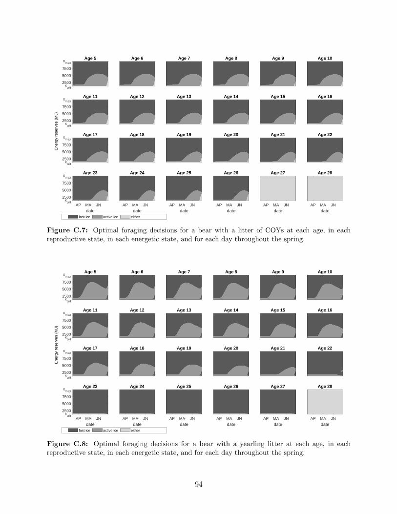
Age 5xmax

7500

5000

2500xcrit

fast ice active ice either

Age 6 Age 7 Age 8 Age 9 Age 10

Age 11

Ene

rgy

rese

rves

(M

J)

xmax

7500

5000

2500xcrit

Age 12 Age 13 Age 14 Age 15 Age 16

Age 17xmax

7500

5000

2500xcrit

Age 18 Age 19 Age 20 Age 21 Age 22

Age 23

AP MA JN

date

xmax

7500

5000

2500xcrit

Age 24

AP MA JN

date

Age 25

AP MA JN

date

Age 26

AP MA JN

date

Age 27

AP MA JN

date

Age 28

AP MA JN

date

Figure C.7: Optimal foraging decisions for a bear with a litter of COYs at each age, in eachreproductive state, in each energetic state, and for each day throughout the spring.

Age 5xmax

7500

5000

2500xcrit

fast ice active ice either

Age 6 Age 7 Age 8 Age 9 Age 10

Age 11

Ene

rgy

rese

rves

(M

J)

xmax

7500

5000

2500xcrit

Age 12 Age 13 Age 14 Age 15 Age 16

Age 17xmax

7500

5000

2500xcrit

Age 18 Age 19 Age 20 Age 21 Age 22

Age 23

AP MA JN

date

xmax

7500

5000

2500xcrit

Age 24

AP MA JN

date

Age 25

AP MA JN

date

Age 26

AP MA JN

date

Age 27

AP MA JN

date

Age 28

AP MA JN

date

Figure C.8: Optimal foraging decisions for a bear with a yearling litter at each age, in eachreproductive state, in each energetic state, and for each day throughout the spring.

94

Chapter 5

Matrix methods for stochastic

dynamic programming in ecology and

evolutionary biology

The work presented in this chapter has been submitted for review: Reimer, J.R., Mangel,

M., Derocher, A.E., and Lewis, M.A. Matrix methods for stochastic dynamic programming

in ecology and evolutionary biology. Two additional appendices, “Glossary of matrix termi-

nology”, and “Helpful R commands” were included in the paper to assist nonexperts, but

are not relevant to this thesis.

5.1 Introduction

Tradeoffs are an unavoidable part of being alive. Tradeoffs may be physiological (e.g., how

much energy to allocate to growth versus reproduction (Rees et al., 1999)), or behavioural

(e.g., how to balance energy gain with predator avoidance (Mangel and Clark, 1986; McNa-

mara and Houston, 1986; Ludwig and Rowe, 1990). What constitutes a successful strategy is

ultimately determined by natural selection, as individuals whose strategies maximize fitness

will pass on heritable parts of this strategy to their offspring.

Similarly, conservationists and wildlife or fisheries managers must also make tradeoffs

while striving to achieve conservation or management goals. In this context, tradeoffs are

often between immediate and future rewards (e.g., how much to harvest now while main-

taining a sufficient population to harvest later (Runge and Johnson, 2002)). The objective

may be to control an invasive species (Bogich and Shea, 2008), ensure the long term viability

of a population, or maintain some threshold of species richness in a region.

95

Optimal control theory addresses how an individual could optimally navigate a series

of risks and rewards while trying to achieve an objective, subject to relevant constraints.

Often, the optimal control will depend on both the state of the individual (e.g., an animal’s

physiological state) and a temporal component (e.g., how many days remain in a season).

We use the word decision (rather than control) to describe the action taken by an individual

whenever there is more than one possible action. These decisions include events beyond

cognition such as the decision by an animal to abort a pregnancy based on their level of

energy reserves. An optimal decision question may be framed as a state-dependent Markov

decision process (Puterman, 1994). Stochastic dynamic programming (SDP) is a common

method to deal with state-dependent Markov decision processes. It is common in both

ecology and resource management to refer to both the model and the method of solving the

model as SDP (Marescot et al., 2013) and we follow this convention. SDP has been used in

many areas of biology, including behavioural biology (McNamara et al., 2001; Mangel, 2015),

evolutionary biology (Parker and Smith, 1990), cell biology (Mangel and Bonsall, 2008), and

conservation and resource management (Walters and Hilborn, 1978; Marescot et al., 2013).

In some applications of SDP, one is interested in the temporal aspects of the optimal

decisions, especially near some terminal time; these are finite time horizon problems. For

example, we may expect an individual to make riskier foraging decisions near the end of a

feeding season (e.g., the polar bear foraging decisions predicted in Chapter 4) or prioritize

reproduction just before reproductive senescence (Rees et al., 1999). In many cases, the

optimal decisions are stationary (i.e., not varying from one time step to the next) when

they are sufficiently far away from the terminal time. In some applications of SDP, these

stationary decisions are used for prediction (Mangel, 1989; Chan and Godfray, 1993; Mangel

et al., 1995; Millner-Gulland, 1997; Lima and Bednekoff, 1999; Shea and Possingham, 2000),

rather than the transient dynamics near the end of the optimization period; we refer to these

as stationary decision problems. Finally, other questions do not concern a finite time period

at all (Venner et al., 2006; Mangel and Bonsall, 2008), but are infinite horizon problems.

For example, managers may wish to maximize the total number of animals that may be

harvested indefinitely (Runge and Johnson, 2002).

Stationary decision problems and infinite horizon problems in biology are often solved

using essentially the same numerical method, though it appears in the literature under

different names: backwards induction or value iteration (Puterman, 1994; Clark and Mangel,

2000). Several software packages have been created to run these numerical routines for a

wide range of applications in an attempt to make SDP more accessible to the biological

community (Lubow, 1995; Marescot et al., 2013), though there is arguably much insight and

greater flexibility available for researchers implementing an SDP model themselves.

96

SDP models are typically constructed component-wise, separately considering an indi-

vidual in each possible state at each time. While this model formulation is fairly intuitive,

it has the downside of requiring complex code to implement, which is difficult to check for

errors. Furthermore, component-wise model formulation hides the elegant mathematical

structure underlying SDP. Analytical results well known in the SDP literature outside of

ecology (Puterman, 1994) depend on this mathematical structure.

In this paper, we propose the use of vector and matrix notation for SDP applications,

allowing for consideration of an individual in all possible states at each time. We use existing

mathematical results (McNamara, 1991; Puterman, 1994) on the asymptotic properties of

SDP models. These results have received little attention in biology, despite their powerful

implications both for finding solutions and biological interpretation. We demonstrate how

formulating an SDP model in this way leads to analytic methods for obtaining optimal

decisions for both stationary decision problems and infinite horizon problems. We provide

step-by-step instructions for implementing these analytic methods for the two canonical

equations of SDP in ecology (Mangel, 2015), illustrating the key steps with a simple example.

The intuition behind these analytic results also allows us to explain non-intuitive transient

oscillating decisions. Our methods have a notable additional benefit. Ecologists interested

in how an optimally behaving individual’s state changes over time typically run thousands

of Monte Carlo simulations (an approximate method). We describe how SDP model con-

struction using matrices allows for easy and computationally fast implementation of Markov

chains (an exact method) rather than Monte Carlo simulations (Mangel and Clark 1988).

We apply these methods to an existing study of host feeding behaviour in parasitic

wasps (Chan and Godfray, 1993), obtaining both analytic stationary decision results as well

as performing a new sensitivity analysis using our analytic method. We also obtain the

probability distribution of realized states using Markov chains.

5.2 Methods

5.2.1 Stochastic dynamic programming

Regardless of application, SDP models contain several key components (Clark and Mangel,

2000). These include discrete time steps t and a time horizon, which may either be finite with

a terminal time T , or infinite. The set of possible state variables x ∈ χ = {x1, . . . , xk} must

be defined, and any relevant constraints on the states included. The actions available to an

individual in a given state at each time must be made explicit. We assume a finite number of

actions available to an individual. The probabilistic state dynamics (e.g., the probability of

97

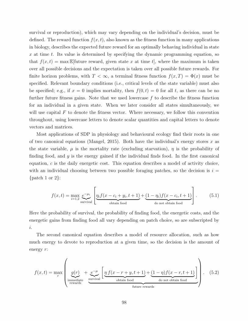
survival or reproduction), which may vary depending on the individual’s decision, must be

defined. The reward function f(x, t), also known as the fitness function in many applications

in biology, describes the expected future reward for an optimally behaving individual in state

x at time t. Its value is determined by specifying the dynamic programming equation, so

that f(x, t) = maxE[future reward, given state x at time t], where the maximum is taken

over all possible decisions and the expectation is taken over all possible future rewards. For

finite horizon problems, with T < ∞, a terminal fitness function f(x, T ) = Φ(x) must be

specified. Relevant boundary conditions (i.e., critical levels of the state variable) must also

be specified; e.g., if x = 0 implies mortality, then f(0, t) = 0 for all t, as there can be no

further future fitness gains. Note that we used lowercase f to describe the fitness function

for an individual in a given state. When we later consider all states simultaneously, we

will use capital F to denote the fitness vector. Where necessary, we follow this convention

throughout, using lowercase letters to denote scalar quantities and capital letters to denote

vectors and matrices.

Most applications of SDP in physiology and behavioural ecology find their roots in one

of two canonical equations (Mangel, 2015). Both have the individual’s energy stores x as

the state variable, µ is the mortality rate (excluding starvation), η is the probability of

finding food, and y is the energy gained if the individual finds food. In the first canonical

equation, c is the daily energetic cost. This equation describes a model of activity choice,

with an individual choosing between two possible foraging patches, so the decision is i =

{patch 1 or 2}:

f(x, t) = maxi=1,2

e−µi⏞⏟⏟⏞survival

⎡⎣ηif(x− ci + yi, t+ 1)⏞ ⏟⏟ ⏞obtain food

+(1− ηi)f(x− ci, t+ 1)⏞ ⏟⏟ ⏞do not obtain food

⎤⎦ . (5.1)

Here the probability of survival, the probability of finding food, the energetic costs, and the

energetic gains from finding food all vary depending on patch choice, so are subscripted by

i.

The second canonical equation describes a model of resource allocation, such as how

much energy to devote to reproduction at a given time, so the decision is the amount of

energy r:

f(x, t) = maxr

⎛⎜⎜⎜⎜⎝ g(r)⏞⏟⏟⏞immediaterewards

+ e−µ⏞⏟⏟⏞survival

[η f(x− r + y, t+ 1)⏞ ⏟⏟ ⏞

obtain food

+(1− η)f(x− r, t+ 1)⏞ ⏟⏟ ⏞do not obtain food

]⏞ ⏟⏟ ⏞

future rewards

⎞⎟⎟⎟⎟⎠ . (5.2)

98

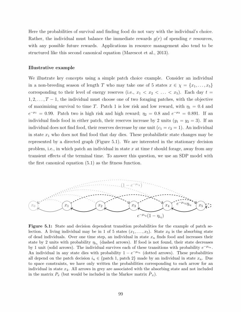
Here the probabilities of survival and finding food do not vary with the individual’s choice.

Rather, the individual must balance the immediate rewards g(r) of spending r resources,

with any possible future rewards. Applications in resource management also tend to be

structured like this second canonical equation (Marescot et al., 2013).

Illustrative example

We illustrate key concepts using a simple patch choice example. Consider an individual

in a non-breeding season of length T who may take one of 5 states x ∈ χ = {x1, . . . , x5}corresponding to their level of energy reserves (i.e., x1 < x2 < . . . < x5). Each day t =

1, 2, . . . , T − 1, the individual must choose one of two foraging patches, with the objective

of maximizing survival to time T . Patch 1 is low risk and low reward, with η1 = 0.4 and

e−µ1 = 0.99. Patch two is high risk and high reward; η2 = 0.8 and e−µ2 = 0.891. If an

individual finds food in either patch, their reserves increase by 2 units (y1 = y2 = 3). If an

individual does not find food, their reserves decrease by one unit (c1 = c2 = 1). An individual

in state x1 who does not find food that day dies. These probabilistic state changes may be

represented by a directed graph (Figure 5.1). We are interested in the stationary decision

problem, i.e., in which patch an individual in state x at time t should forage, away from any

transient effects of the terminal time. To answer this question, we use an SDP model with

the first canonical equation (5.1) as the fitness function.

x0 x1 x2 x3 x4 x5e−µi4ηi4

e−µi4 (1− ηi4)

(1− e−µi4 )

Figure 5.1: State and decision dependent transition probabilities for the example of patch se-lection. A living individual may be in 1 of 5 states (x1, . . . , x5). State x0 is the absorbing stateof dead individuals. Over one time step, an individual in state xn finds food and increases theirstate by 2 units with probability ηin (dashed arrows). If food is not found, their state decreasesby 1 unit (solid arrows). The individual survives each of these transitions with probability e−µin .An individual in any state dies with probability 1 − e−µin (dotted arrows). These probabilitiesall depend on the patch decision in ∈ {patch 1, patch 2} made by an individual in state xn. Dueto space constraints, we have only written the probabilities corresponding to each arrow for anindividual in state x4. All arrows in grey are associated with the absorbing state and not includedin the matrix Pπ (but would be included in the Markov matrix P π).

99

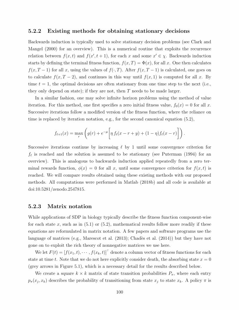
5.2.2 Existing methods for obtaining stationary decisions

Backwards induction is typically used to solve stationary decision problems (see Clark and

Mangel (2000) for an overview). This is a numerical routine that exploits the recurrence

relation between f(x, t) and f(x′, t + 1), for each x and some x′ ∈ χ. Backwards induction

starts by defining the terminal fitness function, f(x, T ) = Φ(x), for all x. One then calculates

f(x, T − 1) for all x, using the values of f(·, T ). After f(x, T − 1) is calculated, one goes on

to calculate f(x, T − 2), and continues in this way until f(x, 1) is computed for all x. By

time t = 1, the optimal decisions are often stationary from one time step to the next (i.e.,

they only depend on state); if they are not, then T needs to be made larger.

In a similar fashion, one may solve infinite horizon problems using the method of value

iteration. For this method, one first specifies a zero initial fitness value, f0(x) = 0 for all x.

Successive iterations follow a modified version of the fitness function, where the reliance on

time is replaced by iteration notation, e.g., for the second canonical equation (5.2),

fℓ+1(x) = maxr

(g(r) + e−µ

[η fℓ(x− r + y) + (1− η)fℓ(x− r)

]).

Successive iterations continue by increasing ℓ by 1 until some convergence criterion for

fℓ is reached and the solution is assumed to be stationary (see Puterman (1994) for an

overview). This is analogous to backwards induction applied repeatedly from a zero ter-

minal rewards function, φ(x) = 0 for all x, until some convergence criterion for f(x, t) is

reached. We will compare results obtained using these existing methods with our proposed

methods. All computations were performed in Matlab (2018b) and all code is available at

doi:10.5281/zenodo.2547815.

5.2.3 Matrix notation

While applications of SDP in biology typically describe the fitness function component-wise

for each state x, such as in (5.1) or (5.2), mathematical results follow more readily if these

equations are reformulated in matrix notation. A few papers and software programs use the

language of matrices (e.g., Marescot et al. (2013); Chades et al. (2014)) but they have not

gone on to exploit the rich theory of nonnegative matrices we use here.

We let F (t) = [f(x1, t), · · · , f(xk, t)]⊤ denote a column vector of fitness functions for each

state at time t. Note that we do not here explicitly consider death, the absorbing state x = 0

(grey arrows in Figure 5.1), which is a necessary detail for the results described below.

We create a square k × k matrix of state transition probabilities Pπ, where each entry

pπ(xj, xk) describes the probability of transitioning from state xj to state xk. A policy π is

100

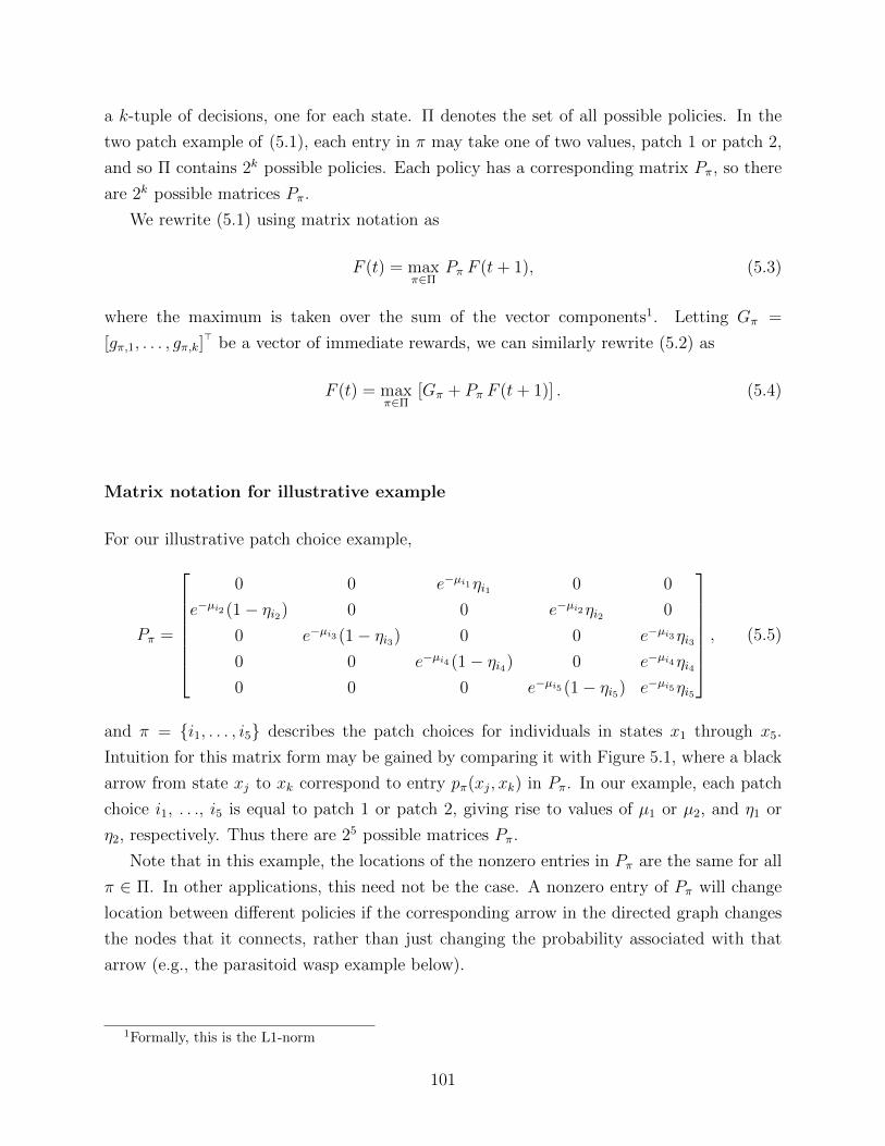
a k-tuple of decisions, one for each state. Π denotes the set of all possible policies. In the

two patch example of (5.1), each entry in π may take one of two values, patch 1 or patch 2,

and so Π contains 2k possible policies. Each policy has a corresponding matrix Pπ, so there

are 2k possible matrices Pπ.

We rewrite (5.1) using matrix notation as

F (t) = maxπ∈Π

Pπ F (t+ 1), (5.3)

where the maximum is taken over the sum of the vector components1. Letting Gπ =

[gπ,1, . . . , gπ,k]⊤ be a vector of immediate rewards, we can similarly rewrite (5.2) as

F (t) = maxπ∈Π

[Gπ + Pπ F (t+ 1)] . (5.4)

Matrix notation for illustrative example

For our illustrative patch choice example,

Pπ =

⎡⎢⎢⎢⎢⎢⎢⎣0 0 e−µi1ηi1 0 0

e−µi2 (1− ηi2) 0 0 e−µi2ηi2 0

0 e−µi3 (1− ηi3) 0 0 e−µi3ηi3

0 0 e−µi4 (1− ηi4) 0 e−µi4ηi4

0 0 0 e−µi5 (1− ηi5) e−µi5ηi5

⎤⎥⎥⎥⎥⎥⎥⎦ , (5.5)

and π = {i1, . . . , i5} describes the patch choices for individuals in states x1 through x5.

Intuition for this matrix form may be gained by comparing it with Figure 5.1, where a black

arrow from state xj to xk correspond to entry pπ(xj, xk) in Pπ. In our example, each patch

choice i1, . . ., i5 is equal to patch 1 or patch 2, giving rise to values of µ1 or µ2, and η1 or

η2, respectively. Thus there are 25 possible matrices Pπ.

Note that in this example, the locations of the nonzero entries in Pπ are the same for all

π ∈ Π. In other applications, this need not be the case. A nonzero entry of Pπ will change

location between different policies if the corresponding arrow in the directed graph changes

the nodes that it connects, rather than just changing the probability associated with that

arrow (e.g., the parasitoid wasp example below).

1Formally, this is the L1-norm

101

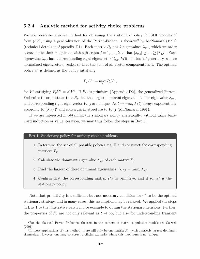
5.2.4 Analytic method for activity choice problems

We now describe a novel method for obtaining the stationary policy for SDP models of

form (5.3), using a generalization of the Perron-Frobenius theorem2 by McNamara (1991)

(technical details in Appendix D1). Each matrix Pπ has k eigenvalues λπ,j, which we order

according to their magnitude with subscripts j = 1, . . . , k so that |λπ,1| ≥ . . . ≥ |λπ,k|. Eacheigenvalue λπ,j has a corresponding right eigenvector Vπ,j. Without loss of generality, we use

normalized eigenvectors, scaled so that the sum of all vector components is 1. The optimal

policy π∗ is defined as the policy satisfying

Pπ∗V ∗ = maxπ

PπV∗,

for V ∗ satisfying PπV∗ = λ∗V ∗. If Pπ∗ is primitive (Appendix D2), the generalized Perron-

Frobenius theorem states that Pπ∗ has the largest dominant eigenvalue3. The eigenvalue λπ∗,1

and corresponding right eigenvector Vπ∗,1 are unique. As t→ −∞, F (t) decays exponentially

according to (λπ∗,1)t and converges in structure to Vπ∗,1 (McNamara, 1991).

If we are interested in obtaining the stationary policy analytically, without using back-

ward induction or value iteration, we may thus follow the steps in Box 1.

Box 1. Stationary policy for activity choice problems

1. Determine the set of all possible policies π ∈ Π and construct the corresponding

matrices Pπ

2. Calculate the dominant eigenvalue λπ,1 of each matrix Pπ

3. Find the largest of these dominant eigenvalues: λπ∗,1 = maxπ λπ,1

4. Confirm that the corresponding matrix Pπ∗ is primitive, and if so, π∗ is the

stationary policy

Note that primitivity is a sufficient but not necessary condition for π∗ to be the optimal

stationary strategy, and in many cases, this assumption may be relaxed. We applied the steps

in Box 1 to the illustrative patch choice example to obtain the stationary decisions. Further,

the properties of Pπ are not only relevant as t → ∞, but also for understanding transient

2For the classical Perron-Frobenius theorem in the context of matrix population models see Caswell(2001).

3In most applications of this method, there will only be one matrix Pπ∗ with a strictly largest dominanteigenvalue. However, one may construct artificial examples where this maximum is not unique.

102

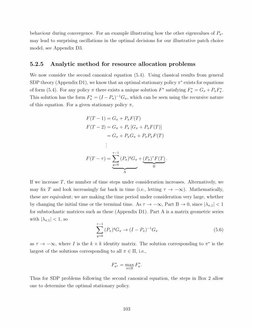
behaviour during convergence. For an example illustrating how the other eigenvalues of Pπ∗

may lead to surprising oscillations in the optimal decisions for our illustrative patch choice

model, see Appendix D3.

5.2.5 Analytic method for resource allocation problems

We now consider the second canonical equation (5.4). Using classical results from general

SDP theory (Appendix D1), we know that an optimal stationary policy π∗ exists for equations

of form (5.4). For any policy π there exists a unique solution F ∗ satisfying F ∗π = Gπ +PπF

∗π .

This solution has the form F ∗π = (I−Pπ)

−1Gπ, which can be seen using the recursive nature

of this equation. For a given stationary policy π,

F (T − 1) = Gπ + PπF (T )

F (T − 2) = Gπ + Pπ [Gπ + PπF (T )]

= Gπ + PπGπ + PπPπF (T )

...

F (T − τ) =τ−1∑q=0

(Pπ)qGπ⏞ ⏟⏟ ⏞

A

+(Pπ)τF (T )⏞ ⏟⏟ ⏞B

.

If we increase T , the number of time steps under consideration increases. Alternatively, we

may fix T and look increasingly far back in time (i.e., letting τ → −∞). Mathematically,

these are equivalent; we are making the time period under consideration very large, whether

by changing the initial time or the terminal time. As τ → −∞, Part B → 0, since |λπ,1| < 1

for substochastic matrices such as these (Appendix D1). Part A is a matrix geometric series

with |λπ,1| < 1, soτ−1∑q=0

(Pπ)qGπ → (I − Pπ)

−1Gπ (5.6)

as τ → −∞, where I is the k × k identity matrix. The solution corresponding to π∗ is the

largest of the solutions corresponding to all π ∈ Π, i.e.,

F ∗π∗ = max

π∈ΠF ∗π .

Thus for SDP problems following the second canonical equation, the steps in Box 2 allow

one to determine the optimal stationary policy.

103

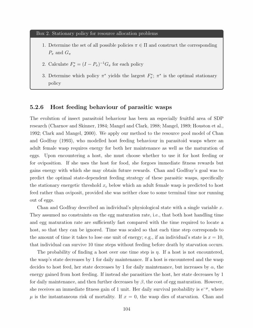
Box 2. Stationary policy for resource allocation problems

1. Determine the set of all possible policies π ∈ Π and construct the corresponding

Pπ and Gπ

2. Calculate F ∗π = (I − Pπ)

−1Gπ for each policy

3. Determine which policy π∗ yields the largest F ∗π ; π

∗ is the optimal stationary

policy

5.2.6 Host feeding behaviour of parasitic wasps

The evolution of insect parasitoid behaviour has been an especially fruitful area of SDP

research (Charnov and Skinner, 1984; Mangel and Clark, 1988; Mangel, 1989; Houston et al.,

1992; Clark and Mangel, 2000). We apply our method to the resource pool model of Chan

and Godfray (1993), who modelled host feeding behaviour in parasitoid wasps where an

adult female wasp requires energy for both her maintenance as well as the maturation of

eggs. Upon encountering a host, she must choose whether to use it for host feeding or

for oviposition. If she uses the host for food, she forgoes immediate fitness rewards but

gains energy with which she may obtain future rewards. Chan and Godfray’s goal was to

predict the optimal state-dependent feeding strategy of these parasitic wasps, specifically

the stationary energetic threshold xc below which an adult female wasp is predicted to host

feed rather than oviposit, provided she was neither close to some terminal time nor running

out of eggs.

Chan and Godfray described an individual’s physiological state with a single variable x.

They assumed no constraints on the egg maturation rate, i.e., that both host handling time

and egg maturation rate are sufficiently fast compared with the time required to locate a

host, so that they can be ignored. Time was scaled so that each time step corresponds to

the amount of time it takes to lose one unit of energy; e.g., if an individual’s state is x = 10,

that individual can survive 10 time steps without feeding before death by starvation occurs.

The probability of finding a host over one time step is η. If a host is not encountered,

the wasp’s state decreases by 1 for daily maintenance. If a host is encountered and the wasp

decides to host feed, her state decreases by 1 for daily maintenance, but increases by α, the

energy gained from host feeding. If instead she parasitizes the host, her state decreases by 1

for daily maintenance, and then further decreases by β, the cost of egg maturation. However,

she receives an immediate fitness gain of 1 unit. Her daily survival probability is e−µ, where

µ is the instantaneous risk of mortality. If x = 0, the wasp dies of starvation. Chan and

104

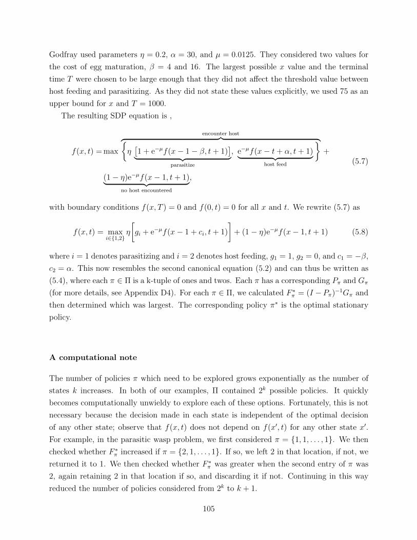
Godfray used parameters η = 0.2, α = 30, and µ = 0.0125. They considered two values for

the cost of egg maturation, β = 4 and 16. The largest possible x value and the terminal

time T were chosen to be large enough that they did not affect the threshold value between

host feeding and parasitizing. As they did not state these values explicitly, we used 75 as an

upper bound for x and T = 1000.

The resulting SDP equation is ,

f(x, t) =max

encounter host⏟ ⏞⏞ ⏟{η[1 + e−µf(x− 1− β, t+ 1)

]⏞ ⏟⏟ ⏞parasitize

, e−µf(x− t+ α, t+ 1)⏞ ⏟⏟ ⏞host feed

}+

(1− η)e−µf(x− 1, t+ 1)⏞ ⏟⏟ ⏞no host encountered

,

(5.7)

with boundary conditions f(x, T ) = 0 and f(0, t) = 0 for all x and t. We rewrite (5.7) as

f(x, t) = maxi∈{1,2}

η

[gi + e−µf(x− 1 + ci, t+ 1)

]+ (1− η)e−µf(x− 1, t+ 1) (5.8)

where i = 1 denotes parasitizing and i = 2 denotes host feeding, g1 = 1, g2 = 0, and c1 = −β,c2 = α. This now resembles the second canonical equation (5.2) and can thus be written as

(5.4), where each π ∈ Π is a k-tuple of ones and twos. Each π has a corresponding Pπ and Gπ

(for more details, see Appendix D4). For each π ∈ Π, we calculated F ∗π = (I −Pπ)

−1Gπ and

then determined which was largest. The corresponding policy π∗ is the optimal stationary

policy.

A computational note

The number of policies π which need to be explored grows exponentially as the number of

states k increases. In both of our examples, Π contained 2k possible policies. It quickly

becomes computationally unwieldy to explore each of these options. Fortunately, this is not

necessary because the decision made in each state is independent of the optimal decision

of any other state; observe that f(x, t) does not depend on f(x′, t) for any other state x′.

For example, in the parasitic wasp problem, we first considered π = {1, 1, . . . , 1}. We then

checked whether F ∗π increased if π = {2, 1, . . . , 1}. If so, we left 2 in that location, if not, we

returned it to 1. We then checked whether F ∗π was greater when the second entry of π was

2, again retaining 2 in that location if so, and discarding it if not. Continuing in this way

reduced the number of policies considered from 2k to k + 1.

105

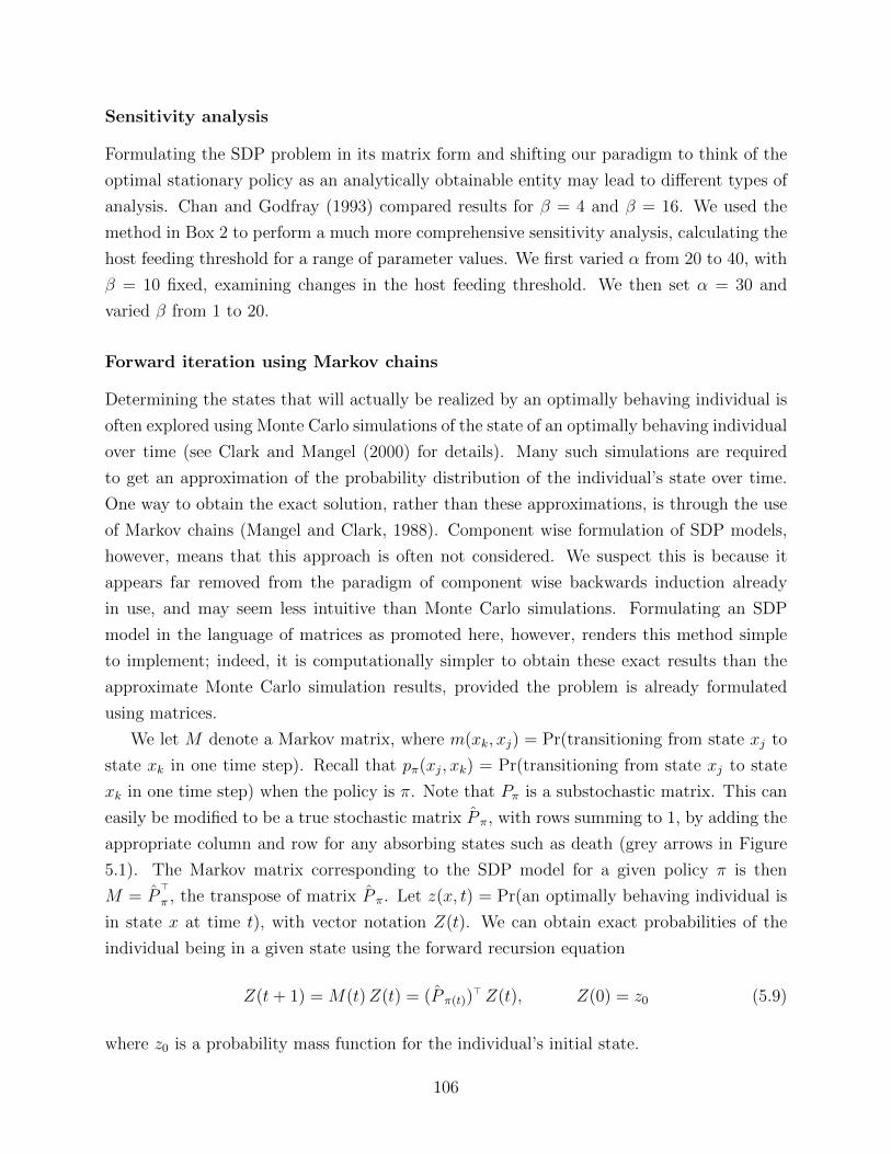
Sensitivity analysis

Formulating the SDP problem in its matrix form and shifting our paradigm to think of the

optimal stationary policy as an analytically obtainable entity may lead to different types of

analysis. Chan and Godfray (1993) compared results for β = 4 and β = 16. We used the

method in Box 2 to perform a much more comprehensive sensitivity analysis, calculating the

host feeding threshold for a range of parameter values. We first varied α from 20 to 40, with

β = 10 fixed, examining changes in the host feeding threshold. We then set α = 30 and

varied β from 1 to 20.

Forward iteration using Markov chains

Determining the states that will actually be realized by an optimally behaving individual is

often explored using Monte Carlo simulations of the state of an optimally behaving individual

over time (see Clark and Mangel (2000) for details). Many such simulations are required

to get an approximation of the probability distribution of the individual’s state over time.

One way to obtain the exact solution, rather than these approximations, is through the use

of Markov chains (Mangel and Clark, 1988). Component wise formulation of SDP models,

however, means that this approach is often not considered. We suspect this is because it

appears far removed from the paradigm of component wise backwards induction already

in use, and may seem less intuitive than Monte Carlo simulations. Formulating an SDP

model in the language of matrices as promoted here, however, renders this method simple

to implement; indeed, it is computationally simpler to obtain these exact results than the

approximate Monte Carlo simulation results, provided the problem is already formulated

using matrices.

We let M denote a Markov matrix, where m(xk, xj) = Pr(transitioning from state xj to

state xk in one time step). Recall that pπ(xj, xk) = Pr(transitioning from state xj to state

xk in one time step) when the policy is π. Note that Pπ is a substochastic matrix. This can

easily be modified to be a true stochastic matrix P π, with rows summing to 1, by adding the

appropriate column and row for any absorbing states such as death (grey arrows in Figure

5.1). The Markov matrix corresponding to the SDP model for a given policy π is then

M = P⊤

π , the transpose of matrix P π. Let z(x, t) = Pr(an optimally behaving individual is

in state x at time t), with vector notation Z(t). We can obtain exact probabilities of the

individual being in a given state using the forward recursion equation

Z(t+ 1) =M(t)Z(t) = (P π(t))⊤ Z(t), Z(0) = z0 (5.9)

where z0 is a probability mass function for the individual’s initial state.

106

We calculated the probability that an individual is in state x at time t for the parasitic

wasp example using this method of Markov chains. We assumed z0 ∼ Poisson(40), β = 16,

and considered t = 1, . . . , 15.

5.3 Results

5.3.1 Illustrative example

In our patch choice example, an individual in each of the 5 states has the same 2 available

patch choices, so there are 25 = 32 possible policies, π1, . . . , π32 (Table 5.1). Each of these

policies corresponds to a matrix Pπ, which takes the form of (5.5). We calculated the

dominant eigenvalue of each of these 32 matrices (Table 5.1) and found the largest of these

dominant eigenvalues was λπ∗,1 = 0.97, corresponding to policy π∗ = {patch 2, patch 2,

patch 1, patch 1, patch 1}. The corresponding matrix is

Pπ∗ =

⎡⎢⎢⎢⎢⎢⎢⎣0 0 0.71 0 0

0.18 0 0 0.71 0

0 0.59 0 0 0.40

0 0 0.59 0 0.40

0 0 0 0.59 0.40

⎤⎥⎥⎥⎥⎥⎥⎦ . (5.10)

policies Ππ1 π2 π3 π4 π5 · · · π∗ · · · π32

patch

choice i1 1 1 1 1 1 2 2

i2 1 1 1 1 1 2 2i3 1 1 1 1 2 · · · 1 · · · 2i4 1 1 2 2 1 1 2i5 1 2 1 2 1 1 2

λπ,1 0.94 0.90 0.94 0.89 0.96 · · · 0.97 · · · 0.89

Table 5.1: All possible policies π (i.e., the patch choice between patch 1 and 2 for an individual ineach of the 5 possible states) and the dominant eigenvalue λπ,1 of each policy’s associated matrixPπ. The stationary policy π∗ is the one with the largest dominant eigenvalue, in grey.

By checking sequentially whether (Pπ∗)ξ is positive for ξ = 1, 2, . . ., we found that (Pπ∗)6

is positive, so Pπ∗ is primitive. Thus the conditions of the generalized Perron-Frobenius

theorem are satisfied and we know that the rewards vector F (t) will asymptotically decay

exponentially according to λtπ∗,1, its structure will tend towards that of the corresponding

107

right eigenvector Vπ∗,1, and policy π∗ is the stationary policy. We confirmed this using the

typical method of backwards induction (Figure 5.2).

5 10 15

time

0.4

0.6

0.8

1.0

F(t

)

5 10 15

time

0.1

0.15

0.2

0.25

norm

aliz

ed F

(t)

5 10 15

time

x1

x2

x3

x4

x5

stat

e

patch 2

patch 1

direction of backwards induction

Figure 5.2: Solution (obtained using backwards induction; arrow at top) of the illustrative patchchoice stochastic dynamic programming example. Top: Asymptotic exponential decay of the fitnessvector F (t) backwards in time, as t becomes further away from the terminal time. The bottom curveis f(x1, t) and the top curve is f(x5, t), with the fitness curves for states x2 to x4 in between. Middle:Normalized solution of F (t) converging backwards in time to the right eigenvector Vπ∗,1 correspond-ing to the stationary policy π∗. Vπ∗,1 is shown with the grey dashed lines. Bottom: Convergencebackwards in time to the stationary policy, π∗ = {patch 2,patch 2,patch 1,patch 1,patch 1}.

5.3.2 Host feeding behaviour of parasitic wasps

Using the method outlined in Box 2, we found that when β = 4, the optimal stationary

policy π∗ is to host feed if x ≤ xc = 27, the stationary threshold, and to parasitize otherwise.

When we increased the cost of egg maturation to β = 16, this threshold increased to xc = 37.

108

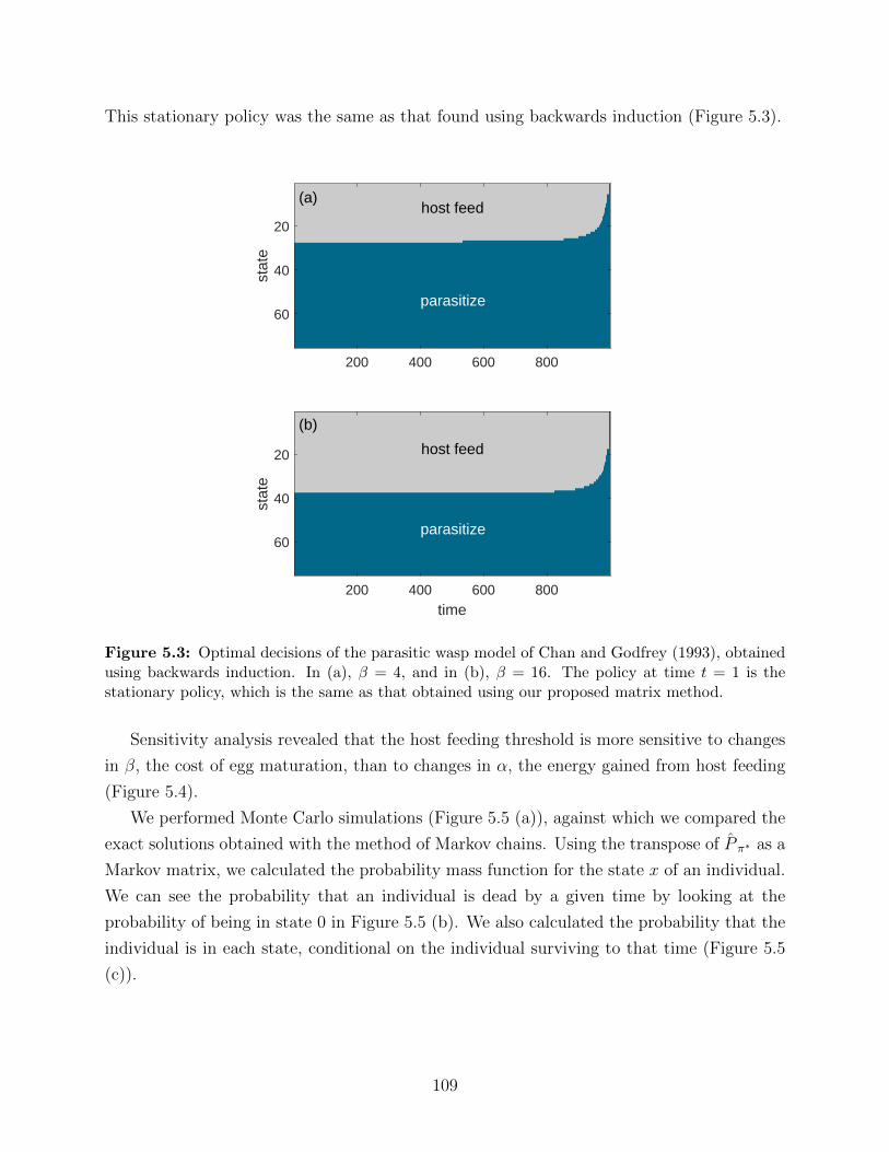
This stationary policy was the same as that found using backwards induction (Figure 5.3).

200 400 600 800

20

40

60

stat

e

200 400 600 800

time

20

40

60

stat

e

parasitize

host feed

parasitize

host feed(a)

(b)

Figure 5.3: Optimal decisions of the parasitic wasp model of Chan and Godfrey (1993), obtainedusing backwards induction. In (a), β = 4, and in (b), β = 16. The policy at time t = 1 is thestationary policy, which is the same as that obtained using our proposed matrix method.

Sensitivity analysis revealed that the host feeding threshold is more sensitive to changes

in β, the cost of egg maturation, than to changes in α, the energy gained from host feeding

(Figure 5.4).

We performed Monte Carlo simulations (Figure 5.5 (a)), against which we compared the

exact solutions obtained with the method of Markov chains. Using the transpose of P π∗ as a

Markov matrix, we calculated the probability mass function for the state x of an individual.

We can see the probability that an individual is dead by a given time by looking at the

probability of being in state 0 in Figure 5.5 (b). We also calculated the probability that the

individual is in each state, conditional on the individual surviving to that time (Figure 5.5

(c)).

109

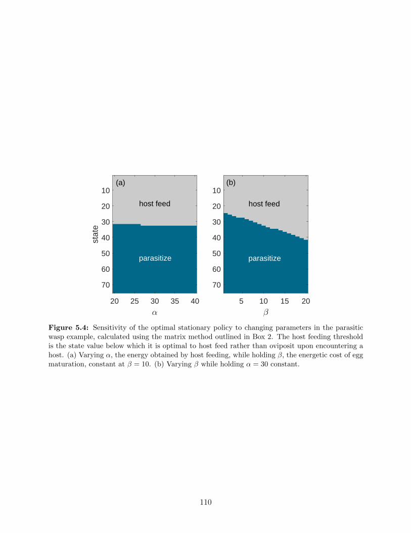
5 10 15 20

10

20

30

40

50

60

70

20 25 30 35 40

10

20

30

40

50

60

70

stat

e

(b)(a)

host feed

parasitize

host feed

parasitize

Figure 5.4: Sensitivity of the optimal stationary policy to changing parameters in the parasiticwasp example, calculated using the matrix method outlined in Box 2. The host feeding thresholdis the state value below which it is optimal to host feed rather than oviposit upon encountering ahost. (a) Varying α, the energy obtained by host feeding, while holding β, the energetic cost of eggmaturation, constant at β = 10. (b) Varying β while holding α = 30 constant.

110

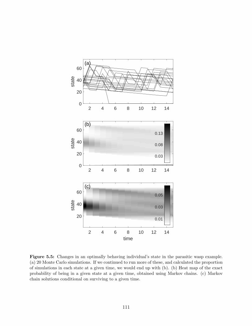
2 4 6 8 10 12 140

20

40

60

stat

e

0.03

0.08

0.13

2 4 6 8 10 12 14time

20

40

60

stat

e

0.01

0.03

0.05

2 4 6 8 10 12 140

20

40

60st

ate

(a)

(b)

(c)

Figure 5.5: Changes in an optimally behaving individual’s state in the parasitic wasp example.(a) 20 Monte Carlo simulations. If we continued to run more of these, and calculated the proportionof simulations in each state at a given time, we would end up with (b). (b) Heat map of the exactprobability of being in a given state at a given time, obtained using Markov chains. (c) Markovchain solutions conditional on surviving to a given time.

111

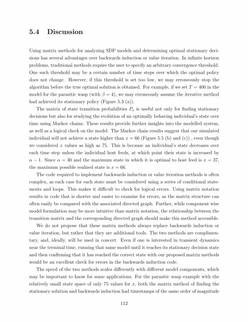
5.4 Discussion

Using matrix methods for analyzing SDP models and determining optimal stationary deci-

sions has several advantages over backwards induction or value iteration. In infinite horizon

problems, traditional methods require the user to specify an arbitrary convergence threshold.

One such threshold may be a certain number of time steps over which the optimal policy

does not change. However, if this threshold is set too low, we may erroneously stop the

algorithm before the true optimal solution is obtained. For example, if we set T = 400 in the

model for the parasitic wasp (with β = 4), we may erroneously assume the iterative method

had achieved its stationary policy (Figure 5.3 (a)).

The matrix of state transition probabilities Pπ is useful not only for finding stationary

decisions but also for studying the evolution of an optimally behaving individual’s state over

time using Markov chains. These results provide further insights into the modelled system,

as well as a logical check on the model. The Markov chain results suggest that our simulated

individual will not achieve a state higher than x = 66 (Figure 5.5 (b) and (c)) , even though

we considered x values as high as 75. This is because an individual’s state decreases over

each time step unless the individual host feeds, at which point their state is increased by

α − 1. Since α = 30 and the maximum state in which it is optimal to host feed is x = 37,

the maximum possible realized state is x = 66.

The code required to implement backwards induction or value iteration methods is often

complex, as each case for each state must be considered using a series of conditional state-

ments and loops. This makes it difficult to check for logical errors. Using matrix notation

results in code that is shorter and easier to examine for errors, as the matrix structure can

often easily be compared with the associated directed graph. Further, while component wise

model formulation may be more intuitive than matrix notation, the relationship between the

transition matrix and the corresponding directed graph should make this method accessible.

We do not propose that these matrix methods always replace backwards induction or

value iteration, but rather that they are additional tools. The two methods are complimen-

tary, and, ideally, will be used in concert. Even if one is interested in transient dynamics

near the terminal time, running that same model until it reaches its stationary decision state

and then confirming that it has reached the correct state with our proposed matrix methods

would be an excellent check for errors in the backwards induction code.

The speed of the two methods scales differently with different model components, which

may be important to know for some applications. For the parasitic wasp example with the

relatively small state space of only 75 values for x, both the matrix method of finding the

stationary solution and backwards induction had timestamps of the same order of magnitude

112

(seconds ×10−2, performed on a modern desktop PC). When we increased T from 1000 to

10000, the computation time for the matrix model did not change at all, while the compu-

tation time for the backwards induction method increased by a factor of ∼10. Conversely,

when we held T = 1000 constant but increased the size of the state space from 75 to 750,

the computation time for the matrix model increased ∼600%, much more dramatically than

for the backwards induction, which increased only ∼4%.

The illustrative models we have considered here were chosen for their simplicity. One

of the benefits of SDP, however, is model flexibility. For example, some SDP applications

include variable time increments, e.g., f(x, t) = f(x, t + τ) + f(x, t + 1) for some integer τ

(Mangel, 1987). Others contain multiple state variables, such as an individual’s size (Brodin

et al., 2017), which would need to be dealt with using either tensors or matrices incorporating

multiple states. This is an area for future work, and will need to be dealt with on a case-by-

case basis, building from the foundations of the two canonical equations.

5.4.1 Conclusion

We have brought attention to several important mathematical results of relevance to eco-

logical applications of SDP. For two canonical equations of SDP in ecology, we used these

mathematical results to analytically obtain the optimal stationary decisions. This relied on

matrix formulations of SDP models. Using matrix formulation of SDP models resulted in

exact solutions for infinite time horizon and stationary decision problems, rather than the

approximate solutions obtained using value iteration or backwards induction. The transition

matrices required for this method allow for easy implementation of Markov chains to study

the probability distribution of an individual’s state.

Appendices

D1 Relevant theory

The Generalized Perron-Frobenius theorem (McNamara, 1991)

McNamara (1991) presented the theorem in the form we have used here, but this result relies

heavily on results from (Sladky, 1976; Grey, 1984; McNamara, 1990).

Consider an equation of the form

λ∗V ∗ = maxπ

PπV∗

113

and define the optimal policy π∗ as that satisfying

Pπ∗V ∗ = maxπ

PπV∗.

If Pπ∗ is primitive (i.e., P ξπ∗ > 0 for some ξ > 0), then the following are true: (i) the domi-

nant eigenvalue λπ∗,1 corresponding to Pπ∗ satisfies λπ∗,1 = maxπ λπ,1, (ii) λπ∗,1 is uniquely

defined and Vπ∗,1 is unique up to multiplication by a constant, (iii) λ∗ = λπ∗,1, and (iv)

limt→−∞(λπ∗,1)−tF (t) ∝ Vπ∗,1.

On the dominant eigenvalue of Pπ

Many of these results rely on the fact that the magnitude of the dominant eigenvalue (i.e.,

the spectral radius) of Pπ is < 1, for all π. We demonstrate this by observing that every term

in matrix Pπ will include a discount term (usually the survival probability of an individual)

in biological applications of SDP. Let

m = mini=1,...,k

e−µi

be the smallest of these discount terms. Provided there is a non-zero mortality rate over

each time step, so µi > 0, then m < 1. If we factor out m, we can rewrite Pπ as Pπ = mP π.

Since P π is a sub-stochastic matrix, with each row summing to ≤ 1, its spectral radius is

≤ 1 (i.e., ρ(P π) ≤ 1). Then

ρ(Pπ) = ρ(mP π) = mρ(P π) < 1.

Existence, uniqueness, and structure of the optimal stationary solution for the

second canonical equation

The following results and their proofs can be found in Puterman (1994). We restate the

relevant theorems here for reference, with notation changed for consistency. The existence of

a unique solution F ∗π for any stationary policy π is guaranteed by Theorem 6.2.5. The form

of this solution for any stationary policy is described in Theorem 6.1.1. The existence of an

optimal stationary policy is guaranteed by Theorem 6.2.10 for an infinite horizon problem

(the analagous theorem for a finite horizon problem can be found in Proposition 4.4.3 in

Puterman (1994)). Theorem 6.2.7c states that this optimal stationary policy has the largest

solution F ∗ out of all possible policies.

Theorem 6.2.5 (Puterman (1994)) Suppose Pπ has a spectral radius < 1, the set of

possible states χ is finite, and the immediate rewards Gπ are bounded for all policies. Then

114

there exists a unique solution F ∗π satisfying F ∗

π = Gπ + PπF∗π .

Theorem 6.1.1 (Puterman (1994)) Suppose Pπ has a spectral radius < 1. Then for any

stationary policy π, F ∗π is the unique solution of

F ∗π = Gπ + PπF

∗π .

Further, F ∗π may be written as

F ∗π = (I − Pπ)

−1Gπ.

Theorem 6.2.10 (Puterman (1994)) Assume the set of possible states χ is discrete and

that the set of possible actions is finite for an individual in each state x ∈ χ. Then there

exists an optimal stationary policy π∗.

Theorem 6.2.7c (Puterman (1994)) Let χ be discrete, then the solution of F ∗π∗ = Gπ∗ +

Pπ∗F ∗π∗ satisfies

F ∗π∗ = max

π∈ΠF ∗π .

D2 Conditions of primitivity

A nonnegative matrix P is primitive if P ξ > 0 for some integer ξ > 0. The primitivity of

a nonnegative matrix can be determined in several different ways (see Caswell (2001), Sec.

4.5.1.2 for a good overview). First, trial and error may yield a suitable ξ such that each of

the entries in P ξ is > 0. Alternatively, primitivity can be assessed graphically by looking at

the directed graph describing probabilistic state changes (e.g., Figure 5.1). A directed graph

(and associated matrix) is irreducible if it is strongly connected—i.e., a path exists from each

node to every other node. An irreducible graph is primitive if the greatest common divisor

of the lengths of those loops is 1 (Rosenblatt, 1957).

D3 Transient oscillating decisions in stochastic dynamic program-

ming

Consider an SDP model with fitness function (5.3), the first canonical equation of SDP

models in biology. Under the conditions outlined in the main text, the stationary policy

π∗ is that corresponding to the matrix Pπ∗ with the largest dominant eigenvalue out of all

possible policies π ∈ Π. For an SDP model with a finite time horizon, this is the policy

which will be optimal as t→ −∞ (i.e., as we get further away from the terminal time).

115

We explore convergence to the stationary policy, using intuition from the theory of matrix

population models (Caswell, 2001). Matrix population models generally take the form N(t+

1) = AN(t). Analogously, we consider a model of the form

F (t) = P F (t+ 1), (5.11)

for some primitive matrix P with a spectral radius < 1 and nonnegative terminal condition

F (T ) with at least one nonzero entry. The solution to (5.11) is

F (T − τ) =k∑

j=1

cjλτjVj

where cj is a scalar, and λj and Vj are eigenvalue and corresponding right eigenvector pairs of

P (Caswell, 2001). Thus the structure of F is influenced initially by the subdominant eigen-

values (i.e., eigenvalues smaller in magnitude than the dominant eigenvalue) and correspond-

ing eigenvectors of P , as τ → ∞. If λj is positive, then the contribution of Vj is exponentially

decreasing (since |λj| < 1, for all j). If −1 < λj < 0, then this term contributes damped os-

cillations with period 2. If λj and λj+1 are complex conjugates, λj = a+bi and λj+1 = a−bi,we may use polar coordinates, so λj = |λj|(cos θ + i sin θ) and λj+1 = |λj|(cos θ − i sin θ).

The contribution of this pair also oscillates, with period 2π/θ (Caswell, 2001).

The damping ratio is defined as ψ = λ1/|λ2| (Caswell, 2001). If ψ is close to 1, a

significant influence from λ2 and V2 will persist for a long time before the dynamics are

asymptotically governed only by λ1 and V1. For increasing values of ψ, the influence of λ2

(and all subsequent eigenvalues) decays increasingly rapidly.

Returning to the SDP model (5.3), these concepts explain the convergence behaviour

of F (t) as t → −∞. For example, if λπ∗,2 is either negative or complex valued, we expect

to see oscillations in the structure of F (t) near the terminal time. If the damping ratio

ψ = λπ∗,1/|λπ∗,2| is close to 1, we expect these oscillations to be apparent for longer than if

the damping ratio is very large. However, unlike in (5.11), the matrix P is not fixed in time.

If the oscillations in the structure of F (t) are sufficiently large—or, analogously, if there exists

another policy π′ and matrix Pπ′ with right eigenvector Vπ′,1 sufficiently similar to Vπ∗,1—the

alternative policy π′ may be optimal periodically, resulting in oscillating decision rules. These

oscillations will continue until the influence of λπ∗,2 is sufficiently small compared to λπ∗,1

and the structure of F (t) is very close to Vπ∗,1. These oscillations can be thought of as an

artifact of not having any cost of switching strategies. We suspect that introducing a small

cost for switching decisions, a kind of behavioral inertia (see, e.g., Dukas and Clark (1995);

Boettiger et al. (2016)), would remove these oscillations. However, for models that do not

116

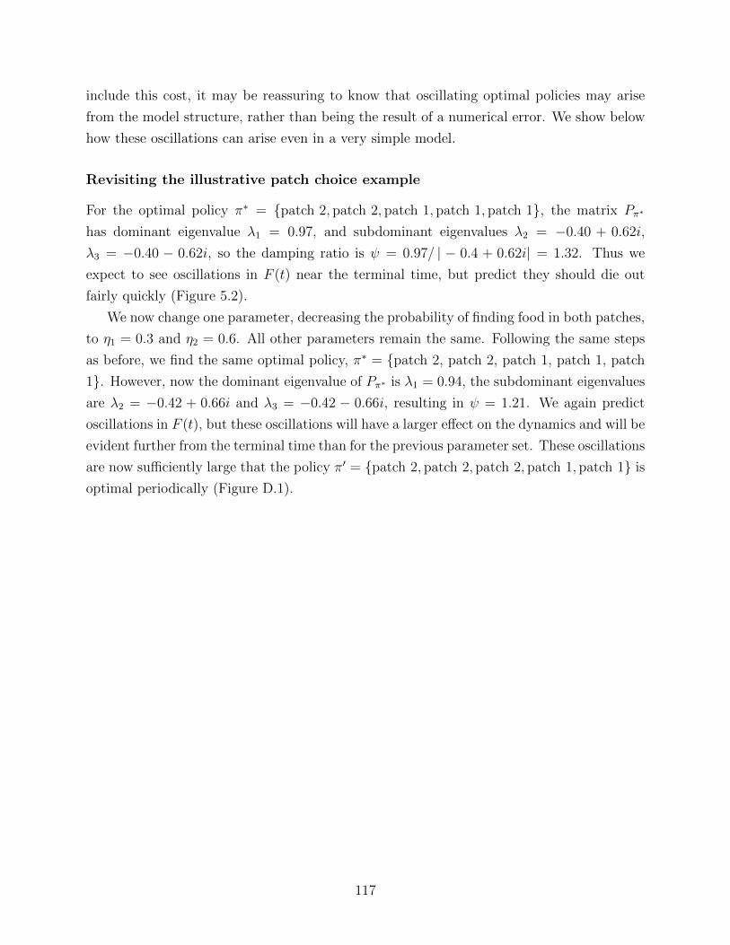
include this cost, it may be reassuring to know that oscillating optimal policies may arise

from the model structure, rather than being the result of a numerical error. We show below

how these oscillations can arise even in a very simple model.

Revisiting the illustrative patch choice example

For the optimal policy π∗ = {patch 2, patch 2, patch 1, patch 1, patch 1}, the matrix Pπ∗

has dominant eigenvalue λ1 = 0.97, and subdominant eigenvalues λ2 = −0.40 + 0.62i,

λ3 = −0.40 − 0.62i, so the damping ratio is ψ = 0.97/ | − 0.4 + 0.62i| = 1.32. Thus we

expect to see oscillations in F (t) near the terminal time, but predict they should die out

fairly quickly (Figure 5.2).

We now change one parameter, decreasing the probability of finding food in both patches,

to η1 = 0.3 and η2 = 0.6. All other parameters remain the same. Following the same steps

as before, we find the same optimal policy, π∗ = {patch 2, patch 2, patch 1, patch 1, patch

1}. However, now the dominant eigenvalue of Pπ∗ is λ1 = 0.94, the subdominant eigenvalues

are λ2 = −0.42 + 0.66i and λ3 = −0.42 − 0.66i, resulting in ψ = 1.21. We again predict

oscillations in F (t), but these oscillations will have a larger effect on the dynamics and will be

evident further from the terminal time than for the previous parameter set. These oscillations

are now sufficiently large that the policy π′ = {patch 2, patch 2, patch 2, patch 1, patch 1} is

optimal periodically (Figure D.1).

117

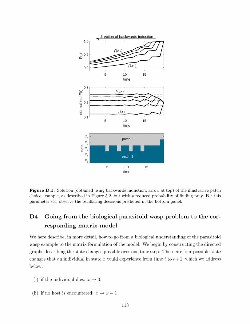
5 10 15time

0.2

0.6

1.0

F(t

)

5 10 15time

0.1

0.2

0.3

norm

aliz

ed F

(t)

5 10 15time

x1

x2

x3

x4

x5

stat

e

patch 2

patch 1

direction of backwards induction

Figure D.1: Solution (obtained using backwards induction; arrow at top) of the illustrative patchchoice example, as described in Figure 5.2, but with a reduced probability of finding prey. For thisparameter set, observe the oscillating decisions predicted in the bottom panel.

D4 Going from the biological parasitoid wasp problem to the cor-

responding matrix model

We here describe, in more detail, how to go from a biological understanding of the parasitoid

wasp example to the matrix formulation of the model. We begin by constructing the directed

graphs describing the state changes possible over one time step. There are four possible state

changes that an individual in state x could experience from time t to t+1, which we address

below:

(i) if the individual dies: x→ 0.

(ii) if no host is encountered: x→ x− 1

118

(iii) if a host is encountered and parasitized: x→ x− 1− β

(iv) if a host is encountered and the individual host feeds: x→ x− 1 + α

(i) Individual dies: x→ 0

The individual has probability (1 − e−µ) of dying over each time step, at which point we

assume x→ 0. In a directed graph, this would be represented by an arrow from each state to

0 (Figure D.2). Note that throughout this section, we do not label every arrow to maintain

readability of the directed graphs, but each arrow of a similar type has the appropriate

similar label.

0 1 2 · · · 75

(1− e−µ)

Figure D.2: (i) Individual dies

For the creation of matrix P , we ignore all processes associated with this absorbing state

and use grey for them in all of our directed graphs to emphasize this point. However, when

we wish to use the method of Markov chains later on, these processes are included in the

Markov matrix.

(ii) No host encountered: x→ x− 1

Regardless of the individual’s state, a host is not encountered with probability (1 − η),

conditional on the individual’s survival (probability e−µ). We represent these probabilities

with arrows going from each state x to state x− 1 in a directed graph (Figure D.3).

0 1 2 · · · 74 75

e−µ(1− η) e−µ(1− η)

Figure D.3: (ii) No host encountered

We now construct the corresponding transition matrix P . Begin with a square matrix

of zeros, with dimensions 75 × 75. The row number corresponds to where the arrows are

leaving “from” and the column number is where the arrows are going “to” in the directed

graph. The transition probability assigned to each arrow in the directed graph going from

119

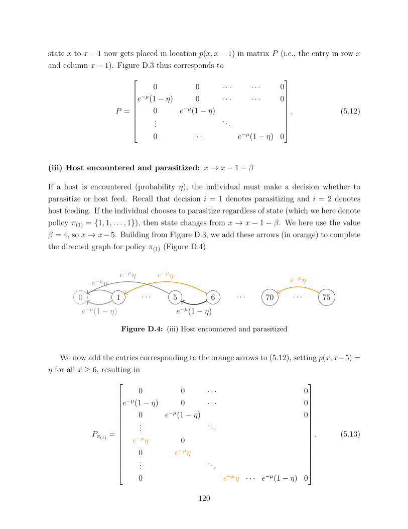
state x to x− 1 now gets placed in location p(x, x− 1) in matrix P (i.e., the entry in row x

and column x− 1). Figure D.3 thus corresponds to

P =

⎡⎢⎢⎢⎢⎢⎢⎢⎣

0 0 · · · · · · 0

e−µ(1− η) 0 · · · · · · 0

0 e−µ(1− η)...

. . .

0 · · · e−µ(1− η) 0

⎤⎥⎥⎥⎥⎥⎥⎥⎦. (5.12)

(iii) Host encountered and parasitized: x→ x− 1− β

If a host is encountered (probability η), the individual must make a decision whether to

parasitize or host feed. Recall that decision i = 1 denotes parasitizing and i = 2 denotes

host feeding. If the individual chooses to parasitize regardless of state (which we here denote

policy π(1) = {1, 1, . . . , 1}), then state changes from x → x − 1 − β. We here use the value

β = 4, so x→ x−5. Building from Figure D.3, we add these arrows (in orange) to complete

the directed graph for policy π(1) (Figure D.4).

0 1 · · · 5 6 · · · 70 · · · 75

e−µ(1− η) e−µ(1− η)

e−µηe−µη e−µη

e−µη

Figure D.4: (iii) Host encountered and parasitized

We now add the entries corresponding to the orange arrows to (5.12), setting p(x, x−5) =

η for all x ≥ 6, resulting in

Pπ(1)=

⎡⎢⎢⎢⎢⎢⎢⎢⎢⎢⎢⎢⎢⎢⎢⎢⎣

0 0 · · · 0

e−µ(1− η) 0 · · · 0

0 e−µ(1− η) 0...

. . .

e−µη 0

0 e−µη...

. . .

0 e−µη · · · e−µ(1− η) 0

⎤⎥⎥⎥⎥⎥⎥⎥⎥⎥⎥⎥⎥⎥⎥⎥⎦. (5.13)

120

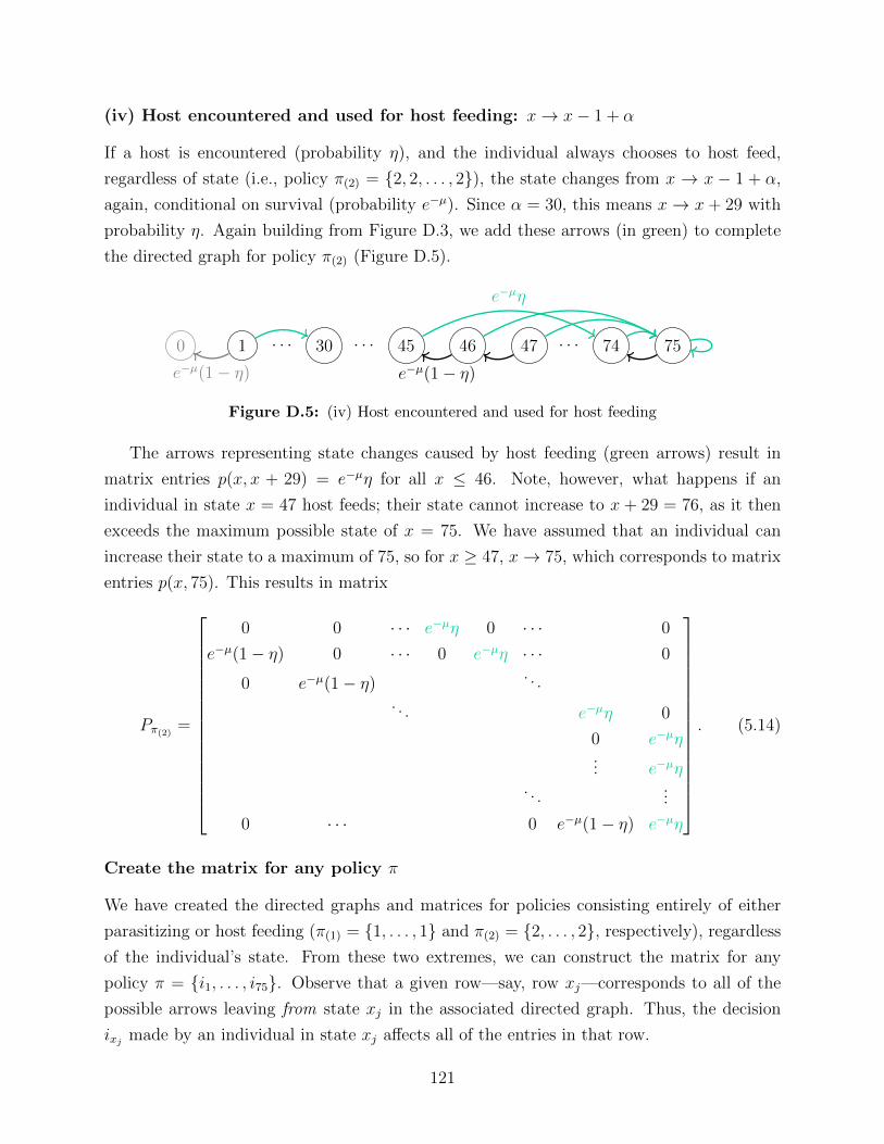
(iv) Host encountered and used for host feeding: x→ x− 1 + α

If a host is encountered (probability η), and the individual always chooses to host feed,

regardless of state (i.e., policy π(2) = {2, 2, . . . , 2}), the state changes from x → x − 1 + α,

again, conditional on survival (probability e−µ). Since α = 30, this means x → x+ 29 with

probability η. Again building from Figure D.3, we add these arrows (in green) to complete

the directed graph for policy π(2) (Figure D.5).

0 1 · · · 30 · · · 45 46 47 · · · 74 75

e−µ(1− η) e−µ(1− η)

e−µη

Figure D.5: (iv) Host encountered and used for host feeding

The arrows representing state changes caused by host feeding (green arrows) result in

matrix entries p(x, x + 29) = e−µη for all x ≤ 46. Note, however, what happens if an

individual in state x = 47 host feeds; their state cannot increase to x + 29 = 76, as it then

exceeds the maximum possible state of x = 75. We have assumed that an individual can

increase their state to a maximum of 75, so for x ≥ 47, x→ 75, which corresponds to matrix

entries p(x, 75). This results in matrix

Pπ(2)=

⎡⎢⎢⎢⎢⎢⎢⎢⎢⎢⎢⎢⎢⎢⎢⎢⎣

0 0 · · · e−µη 0 · · · 0

e−µ(1− η) 0 · · · 0 e−µη · · · 0

0 e−µ(1− η). . .

. . . e−µη 0

0 e−µη... e−µη

. . ....

0 · · · 0 e−µ(1− η) e−µη

⎤⎥⎥⎥⎥⎥⎥⎥⎥⎥⎥⎥⎥⎥⎥⎥⎦. (5.14)

Create the matrix for any policy π

We have created the directed graphs and matrices for policies consisting entirely of either

parasitizing or host feeding (π(1) = {1, . . . , 1} and π(2) = {2, . . . , 2}, respectively), regardlessof the individual’s state. From these two extremes, we can construct the matrix for any

policy π = {i1, . . . , i75}. Observe that a given row—say, row xj—corresponds to all of the

possible arrows leaving from state xj in the associated directed graph. Thus, the decision

ixjmade by an individual in state xj affects all of the entries in that row.

121

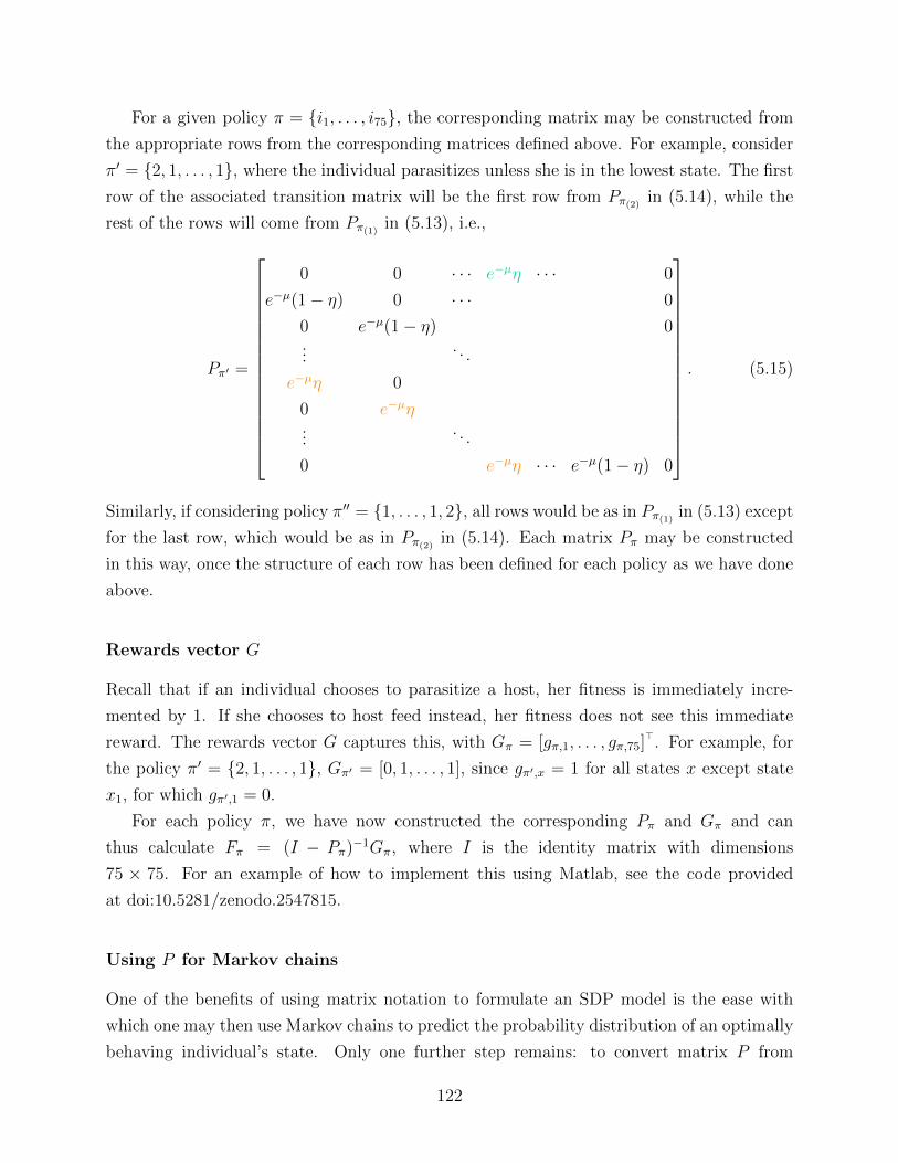
For a given policy π = {i1, . . . , i75}, the corresponding matrix may be constructed from

the appropriate rows from the corresponding matrices defined above. For example, consider

π′ = {2, 1, . . . , 1}, where the individual parasitizes unless she is in the lowest state. The first

row of the associated transition matrix will be the first row from Pπ(2)in (5.14), while the

rest of the rows will come from Pπ(1)in (5.13), i.e.,

Pπ′ =

⎡⎢⎢⎢⎢⎢⎢⎢⎢⎢⎢⎢⎢⎢⎢⎢⎣

0 0 · · · e−µη · · · 0

e−µ(1− η) 0 · · · 0

0 e−µ(1− η) 0...

. . .

e−µη 0

0 e−µη...

. . .

0 e−µη · · · e−µ(1− η) 0

⎤⎥⎥⎥⎥⎥⎥⎥⎥⎥⎥⎥⎥⎥⎥⎥⎦. (5.15)

Similarly, if considering policy π′′ = {1, . . . , 1, 2}, all rows would be as in Pπ(1)in (5.13) except

for the last row, which would be as in Pπ(2)in (5.14). Each matrix Pπ may be constructed

in this way, once the structure of each row has been defined for each policy as we have done

above.

Rewards vector G

Recall that if an individual chooses to parasitize a host, her fitness is immediately incre-

mented by 1. If she chooses to host feed instead, her fitness does not see this immediate

reward. The rewards vector G captures this, with Gπ = [gπ,1, . . . , gπ,75]⊤. For example, for

the policy π′ = {2, 1, . . . , 1}, Gπ′ = [0, 1, . . . , 1], since gπ′,x = 1 for all states x except state

x1, for which gπ′,1 = 0.

For each policy π, we have now constructed the corresponding Pπ and Gπ and can

thus calculate Fπ = (I − Pπ)−1Gπ, where I is the identity matrix with dimensions

75 × 75. For an example of how to implement this using Matlab, see the code provided

at doi:10.5281/zenodo.2547815.

Using P for Markov chains

One of the benefits of using matrix notation to formulate an SDP model is the ease with

which one may then use Markov chains to predict the probability distribution of an optimally

behaving individual’s state. Only one further step remains: to convert matrix P from

122

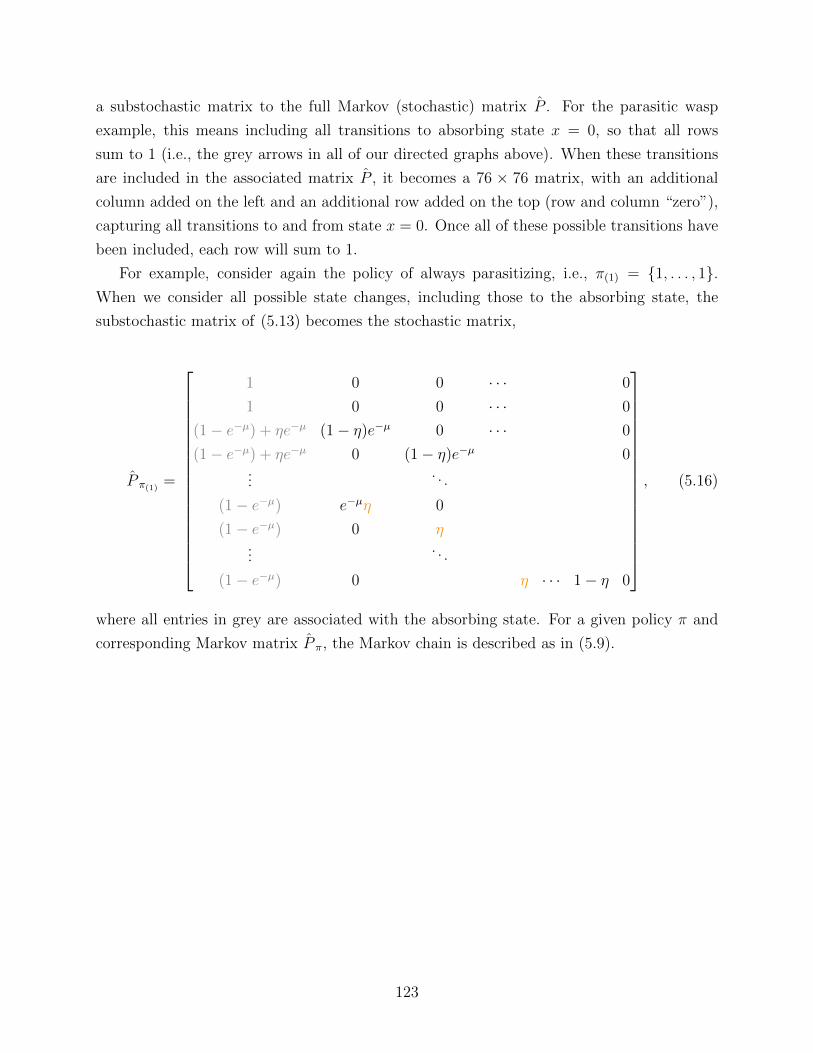
a substochastic matrix to the full Markov (stochastic) matrix P . For the parasitic wasp

example, this means including all transitions to absorbing state x = 0, so that all rows

sum to 1 (i.e., the grey arrows in all of our directed graphs above). When these transitions

are included in the associated matrix P , it becomes a 76 × 76 matrix, with an additional

column added on the left and an additional row added on the top (row and column “zero”),

capturing all transitions to and from state x = 0. Once all of these possible transitions have

been included, each row will sum to 1.

For example, consider again the policy of always parasitizing, i.e., π(1) = {1, . . . , 1}.When we consider all possible state changes, including those to the absorbing state, the

substochastic matrix of (5.13) becomes the stochastic matrix,

P π(1)=

⎡⎢⎢⎢⎢⎢⎢⎢⎢⎢⎢⎢⎢⎢⎢⎢⎢⎢⎣

1 0 0 · · · 0

1 0 0 · · · 0

(1− e−µ) + ηe−µ (1− η)e−µ 0 · · · 0

(1− e−µ) + ηe−µ 0 (1− η)e−µ 0...

. . .

(1− e−µ) e−µη 0

(1− e−µ) 0 η...

. . .

(1− e−µ) 0 η · · · 1− η 0

⎤⎥⎥⎥⎥⎥⎥⎥⎥⎥⎥⎥⎥⎥⎥⎥⎥⎥⎦

, (5.16)

where all entries in grey are associated with the absorbing state. For a given policy π and

corresponding Markov matrix P π, the Markov chain is described as in (5.9).

123

Chapter 6

Discussion

In this thesis, I have contributed to our understanding of Arctic ecology as well as pro-

posed new methods in mathematical ecology. Here I briefly summarize key ecological and

methodological findings, put them in the broader context of contemporary Arctic research

and mathematical ecology, and discuss new questions raised and possible future work.

6.1 Contributions to Arctic ecology

Decadal scale Arctic climate oscillations have historically resulted in periods with colder

winters, thicker sea ice, and a later spring ice breakup (Mysak, 1999). These colder periods

have been linked to reduced ringed seal (Pusa hispida) productivity (Smith, 1987; Harwood

et al., 2012b), and were arguably the most significant environmental stressors on ringed seals

in the western Canadian Arctic over the second half of the 20th century. By synthesizing

existing empirical studies, I provided baseline estimates of ringed seal population growth

rates and population structure during the climate regime of the late 20th century (Chapter

2). Baseline estimates such as these are imperative if we are to predict and detect population

changes.

Since the turn of the century, however, the strength of these climate oscillations has

weakened and new environmental stressors for ringed seals are emerging (Stirling and Smith,

2004; Kelly et al., 2010). The sea ice is thinner, less stable, and is breaking up earlier in the

spring (Dumas et al., 2006; Parkinson, 2014). Further, the annual ice is forming later in the

autumn, and is thus accumulating less snow over the winter (Hezel et al., 2012). While these

environmental trends are well documented, there have been only a few studies of the effects

on ringed seals (Freitas et al., 2008b; Chambellant, 2010; Kelly et al., 2010). By coupling

hypothesized demographic responses of ringed seals to climate model forecasts using a matrix

population model, I explored possible consequences of earlier ice breakup and less snow on

124

the ice for ringed seal pup recruitment (Chapter 2).

While limited information exists about the form of the functional response of ringed seal

recruitment to environmental factors, this data limitation highlights the utility of a modelling

approach in the absence of good empirical data. First, by formalizing hypothesized changes

in ringed seal pup recruitment to reduced snow and early ice breakup, we obtained an idea of

the impact of this hypothesis for estimates of population viability. The dramatic population

declines (50-99% by the end of this century) predicted by coupling the demographic model

to climate forecasts should encourage focused monitoring efforts of this emerging mechanism

of population decline. In addition to changes in population size, the model also predicted

changes in the population structure. Reliable estimates of population size are difficult to

obtain for cryptic species such as ringed seals, so it may be easier to detect changes in

population composition. The current ringed seal monitoring program in the study region

has focused on changes in body condition and ovulation rates (Harwood et al., 2000, 2012b).

Exploring whether the existing monitoring program could also detect the changes I predicted

in population structure, I found that current sample sizes would be insufficient to effectively

detect these changes, and thus proposed consideration of modified or additional monitoring

in this area.

Species with a long history of monitoring, such as polar bears (Ursus maritimus) and

ringed seals, can serve as model species for unexpected ecological phenomena. Even in the

well studied predator-prey relationship between polar bears and seals, I have gained new

insights by applying mathematical modelling methods. Empirical estimates of the relative

abundance of different ages of ringed seals in the spring do not exist. Using matrix popu-

lation models, I approximated the population age structure in the spring and used this to

study which ages of seals polar bears are selecting. While prey switching between species

is a foundational concept in ecology, I have documented the first case of intraspecific prey

switching, with polar bears switching from preying disproportionately on ringed seal pups

in most years, to selecting for mature ringed seals (≥ 21 years old) in years with reduced

pup availability. I expect a similar phenomenon of intraspecific switching may occur in

invertebrate and insect systems, though this has not yet been documented.

One of the challenges of predicting a species’ response to novel climate conditions is the

need to simultaneously account for changes in physiology, behaviour, and environmental

constraints such as the availability of prey. I have taken on this challenge by modelling the

response of a female polar bear to a shortened spring feeding season resulting from earlier

sea ice breakup, using the flexible framework of stochastic dynamic programming (SDP)

(Chapter 4). Reductions in the length of spring feeding increased the amount of risk a

female bear was predicted to tolerate while foraging, as well as shifted predicted reproductive

125

energetic thresholds. While the effects of a one week reduction in the length of a bear’s spring

feeding period may not seem substantial if considering only that year, cumulative effects can

add up to significant declines in lifetime fitness. Unfortunately, small, cumulative effects

such as these are difficult to monitor and for long lived species, such as polar bears, the

effects at the population level may only become apparent over many decades. This study is

the first to use an SDP framework to evaluate the “best case scenario” for a species under

climate change, simultaneously considering both the optimal behavioural and physiological

adaptations an individual could be predicted to assume in new environmental conditions.

In reality, species cannot adapt instantaneously, and do not have perfect knowledge of their

environments, so any fitness declines estimated by this model should be taken as conservative.

The work in Chapter 4 also highlights the way in which polar bears, and other long lived,

k-selected species are likely to experience population decline due to climate change. While

images of starving polar bears may make for better media coverage, in reality, it is more

likely to be reductions in litter size and litter frequency which slowly render the population

unable to replace itself over successive generations.

6.2 Contributions to mathematical ecology

Matrix population models are a foundational tool for modelling population dynamics. These

models can be used to answer a wide variety of questions, and the results of decades of

theoretical work now support increasingly complex analyses. I drew from the theory of

deterministic matrix models, as well as matrix models in periodic and stochastic environ-

ments to study changes in both the size (Chapter 2) and structure of a population of ringed

seals (Chapters 2 and 3). All of these analytic methods assume stationary environmental

conditions. However, on the time scales of interest to many ecological applications, the en-

vironmental changes caused by climate change are nonstationary. Thus, I also used matrix

population models to simulate the population in a nonstationary environment.

While these model results were interesting in their own right, I also used them to conduct

a power analysis to determine whether data collected through current monitoring could be

used to detect projected population changes. Good experimental design often requires spec-

ification of an expected effect size, or some prior knowledge of the parameters one wishes to

observe. Rapid climatic changes may reduce the relevance of previous empirical estimates

of effect size. Mathematical models provide a mechanistic way to estimate the response

of populations or individuals to novel conditions, which can then be used to design more

effective monitoring programs. I have provided an example of this approach (Chapter 2),

and suggest that similar collaborations between applied ecologists and mathematical ecolo-

126

gists could help direct monitoring and experimental efforts in the coming decades of rapid

environmental change.

In addition to the implications for population viability and monitoring, I also found

inconsistencies when I combined demographic parameters into a matrix population model

framework. Documented rates of survival and fertility led to unrealistic population declines

(Chapter 2). Mathematical models may be used to explore the logical implications of existing

studies, highlighting biases or inconsistencies with existing parameter estimates, and help

direct future empirical studies.

Considerable efforts have been made to make both matrix population models and SDP

accessible to ecologists (e.g., the excellent texts of Caswell (2001); Clark and Mangel (2000)).

To make SDP accessible to a biological audience, it is often described component-wise, with

a model equation provided for an individual in each state at each time. While this may be

an intuitive way to present SDP models, this hides the underlying mathematical structure,

which may be represented using nonnegative matrices. In Chapter 5, I have drawn from the

intuition gained from the ergodic theory of matrix population models to provide insights into

the stationary solutions of SDP models. While there is rich mathematical theory for SDP,

it has not been popularized in ecological applications of SDP (but see McNamara (1990,

1991)). I have reformulated the two canonical equations of SDP in ecology and evolution

into matrix notation and then applied relevant mathematical results to these two canonical

equations.

Applying these existing mathematical results to SDP applications in ecology had two

main outcomes. First, the mathematical theory explained the asymptotic behaviour of SDP

models. When solving a component-wise SDP problem using the standard numerical method

of backwards induction, one may observe that–following some transient dynamics near the

terminal time–the fitness function of each state decays exponentially backwards in time.

Further, the structure of the fitness function (i.e., the ratio of the fitness of each state at a

given time to that of a reference state) converges asymptotically backwards in time as well.

The rate of this exponential decay and the asymptotic structure of the fitness function are

both explained by the existing mathematical results, which can be seen once the model is

reformulated into matrix form. Further, the qualitative nature of convergence after the initial

transient period (e.g., oscillations, Appendix D3) can also be explained using properties of

the matrix associated with the stationary policy. Biologically, it is intuitive that the decision

an individual makes should not depend on time if it is sufficiently far away from the terminal

time, but one will likely not infer the exponential form of the decay in fitness or the structure

of the fitness vector if only considering component-wise model formulation.

The second outcome of applying existing mathematical theory to the canonical SDP

127

equations in ecology was that it led to a novel, analytic method for determining stationary

decision rules. This method is useful for obtaining stationary decisions, as well as for error

checking model implementation even if only interested in transient decisions. I have proposed

an analytic method for obtaining the stationary decisions in language intended to be widely

accessible to a broad audience, and provided simple illustrative examples, with the hope

that this method may inform future ecological applications of SDP and the development of

further mathematical results.

6.3 Context of recent scientific advances

The work in this thesis occurs in the broader context of Arctic and mathematical ecology.

Since I began working on these topics, several other notable, relevant scientific and mathe-

matical advancements have been made.

In the past several years, the Arctic has experienced record-breaking heatwaves (Simp-

kins, 2017), and the air temperature in the Arctic has continued to rise at double the rate

of global temperature increase (Overland et al., 2016). As more data is gathered, climate

models continue to be improved upon. The latest round of model results from the Coupled

Model Intercomparison Project (CMIP) will be available by 2020 as part of CMIP6 (Eyring

et al., 2016) (recall that I used climate model outputs from CMIP5 in Chapter 2).

Scientists have continued racing to document and to try to understand the mechanisms

of biological change in the rapidly evolving Arctic (Descamps et al., 2017), in this emerging

so-called “crisis discipline” (Macias-Fauria and Post, 2018). Recent studies of the impacts

of increased Arctic shipping (Hauser et al., 2018) and contaminants in both polar bears

(Tartu et al., 2017; Villa et al., 2017; Liu et al., 2018) and ringed seals (Houde et al., 2017)

add additional complexity to our understanding of the challenges faced by Arctic marine

mammals.

Stable isotope methods have demonstrated plasticity in ringed seal diets (Yurkowski et al.,

2016), and the utility of studying diet shift shifts for understanding changes in the broader

Arctic marine community (Lowther et al., 2017). New methods of data collection (e.g., using

tooth annuli as proxies for body condition) continue to be developed (Nguyen et al., 2017).

Recent changes–both graduated and punctual–in spring ice and snow conditions have allowed

for collection of new data on the response of ringed seal populations (Ferguson et al., 2017).

One recently documented response to reduced sea ice extent is a reduction in spatial overlap

between polar bears and seals in Svalbard. The two species did not change their space use

patterns in the same way in years with reduced ice availability, leading to reduced strength

of their predator-prey relationship (Hamilton et al., 2017).

128

Polar bear science continues to evolve rapidly. Technological advances (e.g., lightweight

cameras and accelerometers) have contributed to better estimates of polar bear metabolic

rates and energy requirements (Pagano et al., 2018). Telemetry methods continue to inform

our understanding of polar bear movement ecology and shifting space use patterns (Lone

et al., 2018b). Telemetry data has advanced our understanding of long-distance swimming

events, and the relationship between swimming and ice conditions (Pilfold et al., 2017; Lone

et al., 2018a). In the Beaufort Sea region, increased sea ice drift linked to climate change is

now thought to cost polar bears an additional 1–3 seals per year due to increased locomotion

(a 2-6.6% increase in annual energy expenditure) (Durner et al., 2017). With a longer ice

free season in this area, more polar bears are now coming ashore in the summer rather than

remaining with the sea ice as it retreats north off of the continental shelf (Pongracz and

Derocher, 2017). During this time on land, Bowhead whale (Balaena mysticetus) remains

may provide a substantial additional food source for polar bears in the area (Rogers et al.,

2015; McKinney et al., 2017; Pongracz and Derocher, 2017). Polar bear food sources other

than seals are of increasing interest as the summer ice free period lengthens in many areas

(Gormezano et al., 2017; Laidre et al., 2018; Stempniewicz, 2017). While more difficult

to observe directly, our understanding of the connection between polar bears and general

marine ecosystem productivity also continues to deepen (Brown et al., 2018; Rode et al.,

2018). In the long-studied region of western Hudson Bay, a population decline of more

than 30% over less than 30 years has been documented (Lunn et al., 2016). In the Chukchi

Sea, the first empirical estimates of vital rates and abundance have been reported Regehr

et al. (2018). The need for further polar bear research–with broader geographic and thematic

scope–remains, and is essential for conservation and evidence-based management (Vongraven

et al., 2018).

Methodological advancements have also been made in the two modelling frameworks used

in this thesis. Matrix population model theory has seen recent progress in our ability to in-

corporate and analyze the effects of population heterogeneity and stochasticity (Hartemink

and Caswell, 2018). Individual heterogeneity may be modelled using second-order matrix

population models, which allow for consideration of both an individual’s current and past

state in predicting their state in the future (de Vries and Caswell, 2017). One may also

simultaneously classify populations by both age and stage (Caswell et al., 2018). New meth-

ods for calculating all moments of an individual’s lifetime reproductive output (van Daalen

and Caswell, 2017), for calculating demographic variance (Caswell and Vindenes, 2018), and

for determining the occupancy times of an individual in a given state (Roth and Caswell,

2018) have also recently been suggested. Matrix population models continue to be a useful

tool for informing management decisions (Rand et al., 2017), and understanding the effects

129

of climate change on populations (Lunn et al., 2016; Jenouvrier et al., 2018).

While ours is the first study to use SDP to examine the effects of anthropogenic climate

change on a species’ behaviour and physiology, recent work has used SDP to study the

effects of other anthropogenic disturbances (e.g., acoustic disturbances) on marine mammals

(McHuron et al., 2017, 2018). SDP continues to be used to understand tradeoffs made by

individual animals as well, including the evolution of facultative hypothermia in small birds

in winter (Brodin et al., 2017) and the evolution of reproductive skipping as an optimal life

history strategy (Griffen, 2018). SDP has seen recent promotion as a tool in applied ecology

for solving adaptive management problems (Chades et al., 2017), and exploring the effect of

management goals (e.g., conserving ecosystem services versus conserving particular species)

on optimal management actions and outcomes (Dee et al., 2017). Recent models also take

into account the different time durations that different management actions may require to

implement (Peron et al., 2017). Ties between SDP and other methods from fields such as

machine learning are also emerging, with applications in biology (Frankenhuis et al., 2018).

6.4 Future work

The work in this thesis leaves many questions unanswered and there are several natural

extensions to this work. Chapter 2 highlighted the need for a better understanding of the

response of ringed seal recruitment to changes in spring snow and ice conditions. As the

Arctic continues to warm in the coming years, studies of the effect of reduced snow and

early ice breakup on ringed seal pups should inform predictions of ringed seal population

level responses. Further, as global climate models continue to improve (e.g., the release of

the new suite of climate models from CMIP6 in the coming years (Eyring et al., 2016)), the

analysis of Chapter 2 should be updated and improved upon.

Chapter 3 examined the historical response of polar bear predation selection to years

with reduced availability of ringed seal pups. Satellite telemetry data have already been

collected for polar bears in the southern Beaufort Sea, and a natural next step would be to

test this location data for our hypothesized switch in spring hunting habitat type in years

known to have reduced availability of ringed seal pups. In the past, these episodic declines in

pup availability were linked to anomalously heavy ice and resultant energetic stress on adult

female ringed seals. Future projections of ringed seal populations may also have punctuated

episodes of low ringed seal pup recruitment, however this will likely be caused by anomalously

early ice breakup. Further work is needed to study the response of polar bear selection to

these changes in the availability of ringed seals.

In Chapter 4, I predicted that a female with cubs will spend more time in the pack ice

130

if the length of the spring feeding season is shortened or if she has poor body condition.

These predictions could be explored in two ways. First, when polar bears are captured in

spring, a measure of their body condition is typically taken, as well as the location of capture.

While this provides just a snapshot in time of that female’s foraging habitat choices, I would

expect that females without any dependent cubs would be caught primarily in more active

ice, while females with dependent cubs captured in the active ice would have worse measures

of body condition than those captured on the landfast ice. The second way to explore these

predictions is again through the use of telemetry data. The type of ice being used by a

female polar bear could be compared to ice breakup date in recent years to see if shorter

spring feeding seasons prompt a shift in foraging behaviour to riskier habitat.

Methodologically, there are several natural extensions to Chapter 5. I have presented

results for the simplest applications of SDP in ecology. However, many applications of SDP

incorporate additional levels of complexity. This method should be extended to include the

following: actions which require multiple time steps to complete; a continuous state vari-

able, requiring interpolation between discrete states; and multiple state variables considered

simultaneously (e.g., an individual’s reproductive and energetic states).

More broadly, the nonstationary nature of climate change illuminates our need for better

tools with which to study transient dynamics and population viability in nonstationary envi-

ronments. This is an active area of research (Ezard et al., 2010; Stott et al., 2011), but much

remains to be done to better understand how individuals, populations, and communities

respond to rapidly evolving environments.

6.5 Conclusion

In this thesis, I have provided insight into both Arctic marine ecology as well as the math-

ematical tools used to study this system. I have provided measurable predictions–a funda-

mental way in which scientific understanding is demonstrated (Houlahan et al., 2017)–of the

response of ringed seals and polar bears to changes in spring environmental conditions. I have

demonstrated the utility of both matrix population models and stochastic dynamic program-

ming as tools with which to formalize and explore existing hypotheses, and generate new

ones. This work has implications for managers trying to effectively monitor environmental

change, for ecologists studying Arctic marine ecology, and for theoretical and mathematical

ecologists interested in links between the ergodic theory of matrix population models and

the asymptotic behaviour of stochastic dynamic programming.

131

Bibliography

Amstrup, S. C. and Durner, G. M. (1995). Survival rates of radio-collared female polar bearsand their dependent young. Can. J. Zool., 73(7):1312–1322.

Amstrup, S. C. and Gardner, C. (1994). Polar bear maternity denning in the Beaufort Sea.J. Wildl. Manage., 58(1):1–10.

Amstrup, S. C., McDonald, T. L., and Stirling, I. (2001). Polar bears in the Beaufort Sea:A 30-Year mark recapture case history. J. Agric. Biol. Environ. Stat., 6:221–234.

Amstrup, S. C., Stirling, I., Smith, T. S., Perham, C., and Thiemann, G. W. (2006). Recentobservations of intraspecific predation and cannibalism among polar bears in the southernBeaufort Sea. Polar Biol., 29(11):997–1002.

Arnould, J. P. Y. and Ramsay, M. a. (1994). Milk production and milk consumption in polarbears during the ice-free period in western Hudson Bay. Can. J. Zool., 72(8):1365–1370.

Arrigo, K. R. (2014). Sea Ice Ecosystems. Ann. Rev. Mar. Sci., 6(1):439–467.

Arrigo, K. R. and van Dijken, G. L. (2015). Continued increases in Arctic Ocean primaryproduction. Prog. Oceanogr., 136:60–70.

Atkinson, S. N. and Ramsay, M. A. (1995). The effects of prolonged fasting of the bodycomposition and reproductive success of female polar bears (Ursus maritimus). Funct.Ecol., 9(4):559–567.

Atwood, T. C., Peacock, E., McKinney, M. A., Lillie, K., Wilson, R., Douglas, D. C., Miller,S., and Terletzky, P. (2016). Rapid environmental change drives increased land use by anArctic marine predator. PLoS One, 11(6):1–18.

Bellman, R. (1957). Dynamic Programming. Princeton University Press, Princeton.

Bentzen, T., Follmann, E., Amstrup, S., York, G., Wooller, M., and O’Hara, T. (2007).Variation in winter diet of southern Beaufort Sea polar bears inferred from stable isotopeanalysis. Can. J. Zool., 85(5):596–608.

Berteaux, D., Humphries, M. M., Krebs, C. J., Lima, M., McAdam, A. G., Pettorelli, N.,Reale, D., Saitoh, T., Tkadlec, E., Weladji, R. B., and Stenseth, N. C. (2006). Constraintsto projecting the effects of climate change on mammals. Clim. Res., 32(2):151–158.

132

Best, R. C. (1977). Ecological aspects of polar bear nutrition. In Proc. 1975 Predat. Symp.,pages 203–211.

Billings, W. and Mooney, H. (1968). The ecology of arctic and alpine plants. Biol. Rev.,43:481–529.

Blix, A. S. and Lentfer, J. W. (1979). Modes of thermal protection in polar bear cubs–atbirth and on emergence from the den. Am. J. Physiol., 236(1):R67–74.

Bluhm, B. A. and Gradinger, R. (2008). Regional variability in food availability for Arcticmarine mammals. Ecol. Appl., 18(2) Supp(2):S77–S96.

Boettiger, C., Bode, M., Sanchirico, J. N., Lariviere, J., Hastings, A., and Armsworth,P. R. (2016). Optimal management of a stochastically varying population when policyadjustment is costly. Ecol. Appl., 26(3):808–817.

Bogich, T. and Shea, K. (2008). A state-dependent model for the optimal management ofan invasive metapopulation. Ecol. Appl., 18(3):748–761.

Brodin, A., Nilsson, J. A., and Nord, A. (2017). Adaptive temperature regulation in thelittle bird in winter: predictions from a stochastic dynamic programming model. Oecologia,185:43–54.

Bromaghin, J. F., McDonald, T. L., Stirling, I., Derocher, A. E., Richardson, E. S., Regehr,E. V., Douglas, D. C., Durner, G. M., Atwood, T. C., and Amstrup, S. C. (2015). Polarbear population dynamics in the southern Beaufort Sea during a period of sea ice decline.Ecol. Appl., 25(3):634–651.

Brown, T. A., Galicia, M. P., Thiemann, G. W., Belt, S. T., Yurkowski, D. J., and Dyck,M. G. (2018). High contributions of sea ice derived carbon in polar bear (Ursus maritimus)tissue. PLoS One, 13(1):1–13.

Burek, K. A., Gulland, F. M. D., and O’Hara, T. M. (2008). Effects of climate change onarctic marine mammal health. Ecol. Appl., 18(2):S126–S134.

Burns, J. J., Kelly, B. P., Aumiller, L. D., Frost, K. J., and Hills, S. (1982). Studies of ringedseals in the Alaskan Beaufort Sea during winter: impacts of seismic exploration. Technicalreport, Alaska Department of Fish and Game, Fairbanks, Alaska.

Caswell, H. (1978). A general formula for the sensitivity of population growth rate to changesin life history parameters. Theor. Popul. Biol., 14:215–230.

Caswell, H. (2001). Matrix Population Models. Sinauer, Sunderland, MA, second edition.

Caswell, H., de Vries, C., Hartemink, N., Roth, G., and van Daalen, S. F. (2018). Age x stage-classified demographic analysis: a comprehensive approach. Ecol. Monogr., 88(4):560–584.

Caswell, H. and John, M. A. (1992). From the individual to the population in demographicmodels. In DeAngelis, D. and Goss, L., editors, Individ. Model. Approaches Ecol., pages36–61. Chapman and Hall, New York.

133

Caswell, H. and Trevisan, M. C. (1994). Sensitivity analysis of periodic matrix models.Ecology, 75(5):1299–1303.

Caswell, H. and Vindenes, Y. (2018). Demographic variance in heterogeneous populations:matrix models and sensitivity analysis. Oikos, 127(5):648–663.

Caswell, H. and Weeks, D. E. (1986). Two-sex models: chaos , extinction , and other dynamicconsequences of sex. Am. Nat., 128(5):707–735.

Chades, I., Chapron, G., Cros, M. J., Garcia, F., and Sabbadin, R. (2014). MDPtoolbox: amulti-platform toolbox to solve stochastic dynamic programming problems. Ecography.,37(9):916–920.

Chades, I., Nicol, S., Rout, T. M., Peron, M., Dujardin, Y., Pichancourt, J. B., Hastings, A.,and Hauser, C. E. (2017). Optimization methods to solve adaptive management problems.Theor. Ecol., 10(1):1–20.

Chambellant, M. (2010). Hudson Bay ringed seal: ecology in a warming climate. A LittleLess Arct. Top Predators World’s Larg. North. Inl. Sea, Hudson Bay, pages 1–308.

Chambellant, M. and Ferguson, S. H. (2009). Comparison of strip- and line-transect samplingto estimate density and abundance of ringed seal (Phoca hispida) in western Hudson Bay,2007 and 2008. Technical report, Fisheries and Oceans Canada.

Chambellant, M., Stirling, I., Gough, W. A., and Ferguson, S. H. (2012). Temporal vari-ations in Hudson Bay ringed seal (Phoca hispida) life-history parameters in relation toenvironment. J. Mammal., 93(1):267–281.

Champely, S. (2015). pwr: Basic Functions for Power Analysis.

Chan, M. S. and Godfray, H. C. (1993). Host-feeding strategies of parasitoid wasps. Evol.Ecol., 7(6):593–604.

Charnov, E. L. and Skinner, S. W. (1984). Evolution of host selection and clutch size inparasitoid wasps. Florida Entomol., 67(1):5–21.

Cherry, S. G., Derocher, A. E., Hobson, K. A., Stirling, I., and Thiemann, G. W. (2011).Quantifying dietary pathways of proteins and lipids to tissues of a marine predator. J.Appl. Ecol., 48(2):373–381.

Cherry, S. G., Derocher, A. E., Stirling, I., and Richardson, E. S. (2009). Fasting physiologyof polar bears in relation to environmental change and breeding behavior in the BeaufortSea. Polar Biol., 32(3):383–391.

Clark, C. W. and Mangel, M. (2000). Dynamic State Variable Models in Ecology. OxfordUniversity Press, New York.

Cohen, J. (1988). Statistical power analysis for the behavioural sciences. Lawrence Erlbaum,Hillsdal, New Jersey, 2nd edition.

134

Cohen, J. E. (1979). Ergodic theorems in demography. Bull. Am. Math. Soc., 1(2):275–295.

Cohen, J. E. and York, N. (1976). Ergodicity of age structure in populations with Markovianvital rates, I: countable states. J. Am. Stat. Assoc., 71:325229.

Comiso, J. C. (2012). Large decadal decline of the Arctic multiyear ice cover. J. Clim.,25(4):1176–1193.

Condon, R. G., Collings, P., andWenzel, G. (1995). The best part of life: subsistence hunting,ethnicity, and economic adaptation among young adult Inuit males. Arctic, 48(1):31–46.

Crawford, J. A., Frost, K. J., Quakenbush, L. T., and Whiting, A. (2012). Different habitatuse strategies by subadult and adult ringed seals (Phoca hispida) in the Bering and Chukchiseas. Polar Biol., 35(2):241–255.

Cresswell, W. (1994). Age-dependent choice of redshank (Tringa totanus) feeding location:profitability or risk? J. Anim. Ecol., 63(3):589–600.

Crouse, D. T., Crowder, L. B., and Caswell, H. (1987). A stage-based population model forloggerhead sea turtles and implications for conservation. Ecology, 68(5):1412–1423.

Cushing, J. (1988). Nonlinear Matrix Models and Population Dynamics. Nat. Resour.Model., 2(4):539–580.

Cushing, J. (1989). A strong ergodic theorem for some nonlinear matrix models for thedynamics of structured populations. Nat. Resour. Model., 3(3):331–357.

de Kroon, H., Plaisier, A., van Groenendael, J., and Caswell, H. (1986). Elasticity: therelative contribution of demographic parameters to population growth rate. Ecology,67(5):1427–1431.

de Vries, C. and Caswell, H. (2017). Demography when history matters: construction andanalysis of second-order matrix population models. Theor. Ecol., pages 1–12.

Dee, L. E., De Lara, M., Costello, C., and Gaines, S. D. (2017). To what extent can ecosystemservices motivate protecting biodiversity? Ecol. Lett., 20(8):935–946.

Derocher, A. and Stirling, I. (1996). Aspects of survival in juvenile polar bears. Can. J.Zool., 74(7):1246–1252.

Derocher, A. E., Andersen, M., Wiig, Ø., and Aars, J. (2010). Sexual dimorphism and themating ecology of polar bears (Ursus maritimus) at Svalbard. Behav. Ecol. Sociobiol.,64(6):939–946.

Derocher, A. E., Andriashek, D., and Arnould, J. P. Y. (1993). Aspects of milk compositionand lactation in polar bears. Can. J. Zool., 71(3):561–567.

Derocher, A. E. and Stirling, I. (1994). Age-specific reproductive performance of femalepolar bears (Ursus maritimus). J. Zool., 234:527–536.

135

Derocher, A. E. and Stirling, I. (1998). Geographic variation in growth of polar bears (Ursusmaritimus). J. Zool., 245(1998):65–72.

Derocher, A. E., Stirling, I., and Andriashek, D. (1992). Pregnancy rates and serum proges-terone levels of polar bears in western Hudson Bay. Can. J. Zool., 70(3):561–566.

Derocher, A. E. and Wiig, Ø. (1999). Infanticide and cannibalism of juvenile polar bears(Ursus maritimus) in Svalbard. Arctic, 52(3):307–310.

Derocher, A. E., Wiig, Ø., and Andersen, M. (2002). Diet composition of polar bears inSvalbard and the western Barents Sea. Polar Biol., 25(6):448–452.

Descamps, S., Aars, J., Fuglei, E., Kovacs, K. M., Lydersen, C., Pavlova, O., Pedersen, A.,Ravolainen, V., and Strøm, H. (2017). Climate change impacts on wildlife in a High Arcticarchipelago—Svalbard, Norway. Glob. Chang. Biol., 23(2):490–502.

Dowsley, M. (2009). Inuit-organised polar bear sport hunting in Nunavut territory, Canada.J. Ecotourism, 8(2):161–175.

Dukas, R. and Clark, C. W. (1995). Searching for cryptic prey: a dynamic model. Ecology,76(4):1320–1326.

Dumas, J. A., Flato, G. M., and Brown, R. D. (2006). Future projections of landfast icethickness and duration in the Canadian Arctic. J. Clim., 19(20):5175–5189.

Durner, G. M., Douglas, D. C., Albeke, S. E., Whiteman, J. P., Amstrup, S. C., Richardson,E., Wilson, R. R., and Ben-David, M. (2017). Increased Arctic sea ice drift alters adultfemale polar bear movements and energetics. Glob. Chang. Biol., 23(9):3460–3473.

Durner, G. M., Douglas, D. C., Nielsen, R. M., Amstrup, S. C., McDonald, T. L., Stirling,I., Mauritzen, M., Born, E. W., Wiig, Ø., DeWeaver, E., Serreze, M. C., Belikov, S. E.,Holland, M. M., Maslanik, J., Aars, J., Bailey, D. A., and Derocher, A. E. (2009). Pre-dicting 21-st century polar bear habitat distribution from global climate models. Ecol.Monogr., 79(1):25–58.

Etkin, D. (1991). Break-up in Hudson Bay: its sensitivity to air temperatures and implica-tions for climate warming. Climatol. Bull., 25:21–34.

Evans, M. R. (2012). Modelling ecological systems in a changing world. Philos. Trans. R.Soc. B Biol. Sci., 367(1586):181–190.

Eyring, V., Bony, S., Meehl, G. A., Senior, C. A., Stevens, B., Stouffer, R. J., and Taylor,K. E. (2016). Overview of the Coupled Model Intercomparison Project Phase 6 (CMIP6)experimental design and organization. Geosci. Model Dev., 9(5):1937–1958.

Ezard, T. H., Bullock, J. M., Dalgleish, H. J., Millon, A., Pelletier, F., Ozgul, A., and Koons,D. N. (2010). Matrix models for a changeable world: the importance of transient dynamicsin population management. J. Appl. Ecol., 47(3):515–523.

136

Ferguson, S. H., Stirling, I., and McLoughlin, P. (2005). Climate change and ringed seal(Phoca hispida) recruitment in western Hudson Bay. Mar. Mammal Sci., 21(1):121–135.

Ferguson, S. H., Young, B. G., Yurkowski, D. J., Anderson, R., Willing, C., and Nielsen, O.(2017). Demographic, ecological and physiological responses of ringed seals to an abruptdecline in sea ice availability. PeerJ, 5:e2957.

Forest, A., Tremblay, J.-E., Gratton, Y., Martin, J., Gagnon, J., Darnis, G., Sampei, M.,Fortier, L., Ardyna, M., Gosselin, M., Hattori, H., Nguyen, D., Maranger, R., Vaque, D.,Marrase, C., Pedros-Alio, C., Sallon, A., Michel, C., Kellogg, C., Deming, J., Shadwick,E., Thomas, H., Link, H., Archambault, P., and Piepenburg, D. (2011). Biogenic carbonflows through the planktonic food web of the Amundsen Gulf (Arctic Ocean): A synthesisof field measurements and inverse modeling analyses. Prog. Oceanogr., 91(4):410–436.

Fossheim, M., Primicerio, R., Johannesen, E., Ingvaldsen, R. B., Aschan, M. M., and Dolgov,A. V. (2015). Recent warming leads to a rapid borealization of fish communities in theArctic. Nat. Clim. Chang., 5(7):673–677.

Frankenhuis, W. E., Panchanathan, K., and Barto, A. G. (2018). Enriching behavioralecology with reinforcement learning methods. Behav. Processes, (January):0–1.

Freitas, C., Kovacs, K. M., Ims, R. A., Fedak, M. A., and Lydersen, C. (2008a). Ringed sealpost-moulting movement tactics and habitat selection. Oecologia, 155(1):193–204.

Freitas, C., Kovacs, K. M., Ims, R. A., and Lydersen, C. (2008b). Predicting habitat use byringed seals (Phoca hispida) in a warming Arctic. Ecol. Modell., 217(1-2):19–32.

Frost, K. J. (1985). The ringed seal (Phoca hispida). In Burns, J. J., Frost, K. J., and Lowry,L. F., editors, Mar. Mamm. species accounts, pages 79–87. Alaska Department of Fish andGame, Game Tech. Bull. 7, Juneau, Alaska.

Galley, R. J., Key, E., Barber, D. G., Hwang, B. J., and Ehn, J. K. (2008). Spatial andtemporal variability of sea ice in the southern Beaufort Sea and Amundsen Gulf: 1980-2004. J. Geophys. Res. Ocean., 113(5):1–18.

Gittleman, J. and Oftedal, O. (1987). Comparative growth and lactation energetics incarnivores. Symp. Zool. Soc. L., 57:41–77.

Gormezano, L. J., Ellis-felege, S. N., Iles, D. T., and Rockwell, R. F. (2017). Polar bearforaging behavior during the ice-free period in western Hudson Bay: observations, origins,and potential significance. BioOne, 3885:1–28.

Greenwood, J. J. (1984). The functional basis of frequency dependent food selection. Biol.J. Linn. Soc., 23(2-3):177–199.

Gremillet, D., Fort, J., Amelineau, F., Zakharova, E., Le Bot, T., Sala, E., and Gavrilo, M.(2015). Arctic warming: nonlinear impacts of sea-ice and glacier melt on seabird foraging.Glob. Chang. Biol., 21(3):1116–1123.

137

Grey, D. R. (1984). Non-negative matrices, dynamic programming and a harvesting problem.J. Appl. Probab., 21(4):685–694.

Griffen, B. D. (2018). Reproductive skipping as an optimal life history strategy in thesouthern elephant seal, Mirounga leonina. Ecol. Evol., (July):1–13.

Hamilton, C. D., Kovacs, K. M., Ims, R. A., Aars, J., and Lydersen, C. (2017). An Arcticpredator-prey system in flux: climate change impacts on coastal space use by polar bearsand ringed seals. J. Anim. Ecol., 86(5):1054–1064.

Hamilton, C. D., Lydersen, C., Ims, R. A., and Kovacs, K. M. (2015). Predictions replacedby facts: a keystone species’ behavioural responses to declining arctic sea-ice. Biol. Lett.,11(20150803):1–6.

Hammill, M., Lydersen, C., Ryg, M., and Smith, T. (1991). Lactation in the ringed seal(Phoca hispida). Can. J. Fish. Aquat. Sci., 48(12):0–5.

Hammill, M. O. (1987). Ecology of the ringed seal (Phoca hispida) in the fast-ice of BarrowStrait, Northwest Territories. PhD thesis, College of McGill Univ.

Hammill, M. O. and Smith, T. G. (1989). Factors affecting the distribution and abundance ofringed seal structures in Barrow Strait, Northwest Territories. Can. J. Zool., 67(9):2212–2219.

Hammill, M. O. and Smith, T. G. (1991). The role of predation in the ecology of the ringedseal in Barrow Strait, Northwest Territories, Canada. Mar. Mammal Sci., 7:123–135.

Harding, K. C., Harkonen, T., Helander, B., and Karlsson, O. (2007). Status of Baltic greyseals: population assessment and extinction risk. NAMMCO Sci. Publ., 6:33–56.

Harkonen, T. and Heide-Jørgensen, M. P. (1990). Comparative life histories of East Atlanticand other harbour seal populations. Ophelia, 32(3):211–235.

Hartemink, N. and Caswell, H. (2018). Variance in animal longevity: contributions of het-erogeneity and stochasticity. Popul. Ecol., 60(1-2):89–99.

Harvey, J. A., Van Den Berg, D., Ellers, J., Kampen, R., Crowther, T. W., Roessingh,P., Verheggen, B., Nuijten, R. J., Post, E., Lewandowsky, S., Stirling, I., Balgopal, M.,Amstrup, S. C., and Mann, M. E. (2018). Internet blogs, polar bears, and climate-changedenial by proxy. Bioscience, 68(4):281–287.

Harwood, L., Smith, T., and Melling, H. (2000). Reproduction and body condition of theringed seal (Phoca hispida) in the eastern Beaufort Sea, NT, Canada, as assessed througha harvest-based sampling program. Arctic, 53(4):422–431.

Harwood, L. A., Smith, T. G., and Auld, J. C. (2012a). Fall Migration of Ringed Seals(Phoca hispida) through the Beaufort and Chukchi Seas, 2001-02. Arctic, 65(1):35–44.

138

Harwood, L. A., Smith, T. G., George, J. C., Sandstrom, S. J., Walkusz, W., and Divoky,G. J. (2015). Change in the Beaufort Sea ecosystem: diverging trends in body conditionand/or production in five marine vertebrate species. Prog. Oceanogr., 136(October):263–273.

Harwood, L. A., Smith, T. G., Melling, H., Alikamik, J., and Kingsley, M. C. S. (2012b).Ringed seals and sea ice in Canada’s western Arctic: harvest-based monitoring 1992–2011.Arctic, 65(4):377–390.

Harwood, L. a. and Stirling, I. (1992). Distribution of ringed seals in the southeasternBeaufort Sea during late summer. Can. J. Zool., 70(5):891–900.

Hassol, S. J. (2004). Impacts of a warming Arctic: Arctic climate impact assessment. Tech-nical report, Cambridge University Press, Cambridge, UK.

Hastings, A. (1983). Age-dependent predation is not a simple process. I. Continuous timemodels. Theor. Popul. Biol., 23(3):347–362.

Hastings, A. (1984). Age-dependent predation is not a simple process. II. Wolves, ungulates,and a discrete time model for predation on juveniles with a stabilizing tail. Theor. Popul.Biol., 26(2):271–282.

Hauser, D. D. W., Laidre, K. L., and Stern, H. L. (2018). Vulnerability of Arctic marinemammals to vessel traffic in the increasingly ice-free Northwest Passage and Northern SeaRoute. Proc. Natl. Acad. Sci., 115(29):7617–7622.

Heppell, S. S., Caswell, H., and Crowder, L. B. (2000). Life histories and elasticity patterns:perturbation analysis for species with minimal demographic data. Ecology, 81(3):654–665.

Herreman, J. and Peacock, E. (2013). Polar bear use of a persistent food subsidy: insightsfrom non-invasive genetic sampling in Alaska. Ursus, 24(2):148–163.

Hezel, P. J., Zhang, X., Bitz, C. M., Kelly, B. P., and Massonnet, F. (2012). Projecteddecline in spring snow depth on Arctic sea ice caused by progressively later autumn openocean freeze-up this century. Geophys. Res. Lett., 39(17):1–8.

Holbrook, S. J. and Schmitt, R. J. (1988). The combined effects of predation risk and foodreward on patch selection. Ecology, 69(1):125–134.

Holst, M., Stirling, I., and Calvert, W. (1999). Age structure and reproductive rates ofringed seals (Phoca hispida) on the northwestern coast of Hudson Bay in 1991 and 1992.Mar. Mammal Sci., 15(4):1357–1364.

Hop, H. and Gjøsæter, H. (2013). Polar cod (Boreogadus saida) and capelin (Mallotusvillosus) as key species in marine food webs of the Arctic and the Barents Sea. Mar. Biol.Res., 9(9):878–894.

139

Houde, M., Wang, X., Ferguson, S. H., Gagnon, P., Brown, T. M., Tanabe, S., Kunito,T., Kwan, M., and Muir, D. C. (2017). Spatial and temporal trends of alternative flameretardants and polybrominated diphenyl ethers in ringed seals (Phoca hispida) across theCanadian Arctic. Environ. Pollut., 223:266–276.

Houlahan, J. E., McKinney, S. T., Anderson, T. M., and McGill, B. J. (2017). The priorityof prediction in ecological understanding. Oikos, 126(1):1–7.

Houston, A. I. and Mcnamara, J. M. (1993). A theoretical investigation of the fat reservesand mortality levels of small birds in winter. Ornis Scand., 24(3):205–219.

Houston, A. I. and McNamara, J. M. (1999). Models of adaptive behaviour: an approachbased on state. Cambridge University Press.

Houston, A. I., McNamara, J. M., and Godfray, H. C. J. (1992). The effect of variability onhost feeding and reproductive success in parasitoids. Bull. Math. Biol., 54(2-3):465–476.

Hubbard, S. F., Cook, R. M., Glover, J. G., and Greenwood, J. (1982). Apostatic selectionas an optimal foraging strategy. J. Anim. Ecol., 1051(2):625–633.

Hughes, R. and Croy, M. (1993). An experimental analysis of frequency-dependent predation(switching) in the 15-spined stickleback, Spinachia spinachia. J. Anim. Ecol., 62:341–352.

Hunter, C. M., Caswell, H., Runge, M. C., Regehr, E. V., Amstrup, S. C., and Stirling, I.(2007). Polar bears in the southern Beaufort Sea II: demography and population growthin relation to sea ice conditions. U.S Geol. Surv., 1:1–46.

Hunter, C. M., Caswell, H., Runge, M. C., Regehr, E. V., Steve, C., and Stirling, I. (2010).Climate change threatens polar bear populations: a stochastic demographic analysis. Ecol-ogy, 91(10):2883–2897.

Iacozza, J. and Ferguson, S. H. (2014). Spatio-temporal variability of snow over sea ice inwestern Hudson Bay, with reference to ringed seal pup survival. Polar Biol., 37(6):817–832.

IPCC (2014). Summary for Policymakers. Technical report, IPCC, Geneva, Switzerland.

IUCN Polar Bear Specialist Group (2017a). IUCN/SSC PBSG - Polar bear population map.

IUCN Polar Bear Specialist Group (2017b). IUCN/SSC PBSG Population Status - NorthernBeaufort Sea (NB).

IUCN Polar Bear Specialist Group (2017c). IUCN/SSC PBSG Population Status - SouthernBeaufort Sea (SB).

Jenouvrier, S., Caswell, H., Barbraud, C., Holland, M., Strœve, J., and Weimerskirch, H.(2009). Demographic models and IPCC climate projections predict the decline of anemperor penguin population. Proc. Natl. Acad. Sci., 106(6):1844–1847.

140

Jenouvrier, S., Desprez, M., Fay, R., Barbraud, C., Weimerskirch, H., Delord, K., andCaswell, H. (2018). Climate change and functional traits affect population dynamics of along-lived seabird. J. Anim. Ecol., 87(4):906–920.

Kelly, B. P. (1988). Ringed seal, Phoca hispida. In Lentifer, J. W., editor, Sel. Mar. MammalSpecies Alaska Species Accounts with Res. Manag. Recomm., pages 57–75. Marine MammalCommission, Washington, D.C.

Kelly, B. P., Bengston, J. L., Boveng, P. L., Cameronm, M. F., Dahle, S. P., Jansen, J. K.,Logerwell, E. A., Overland, J. E., Sabine, L. C., and Wilder, J. M. (2010). Status Reviewof the Ringed Seal (Phoca hispida). Technical report, Department of Commerce UnitedStates of America.

Kelly, B. P. and Quakenbush, L. T. (1990). Spatiotemporal use of lairs by ringed seals (Phocahispida). Can. J. Zool., 68(12):2503–2512.

King, J. R. and Murphy, M. E. (1985). Periods of nutritional stress in the annual cycle ofendotherms: fact or fiction? Am. Zool., 25(May):955–964.

Kingsley, M. (1984). The abundance of ringed seals in the Beaufort Sea and Amundsen Gulf,1983. Can. Manuscr. Rep. Fish. Aquat. Sci., 1778(1778):1–8.

Kingsley, M. C. S. and Byers, T. J. (1998). Failure in reproduction in ringed seals (Phocahispida) in Amundsen Gulf, Northwest Territories in 1984-1987. In Heide-Jorgensen, M. P.and Lydersen, C., editors, Ringed seals North Atl., pages 197–2010. NAMMCO ScientificPublications, Tromso.

Klaassen, M. (2003). Relationships between migration and breeding strategies in arcticbreeding birds. In Berthold, P., Gwinner, E., and Sonnenschein, E., editors, Avian Migr.,pages 237–249. Springer-Verlag, Berlin.

Klein, D. R. (1990). Variation in quality of caribou and reindeer forage plants associatedwith season, plant part, and phenology. Rangifer, 10(3):123.

Kot, M. (2001). Elements of Mathematical Ecology. Cambridge University Press, Cambridge,UK.

Kovacs, K. M., Lydersen, C., Overland, J. E., and Moore, S. E. (2011). Impacts of changingsea-ice conditions on Arctic marine mammals. Mar. Biodivers., 41(1):181–194.

Lack, D. (1947). The significance of clutch-size. Ibis (Lond. 1859)., 89(2):302–352.

Laidre, K. L., Stern, H., Kovacs, K. M., Lowry, L., Moore, S. E., Regehr, E. V., Fergu-son, S. H., Wiig, Ø., Boveng, P., Angliss, R. P., Born, E. W., Litovka, D., Quakenbush,L., Lydersen, C., Vongraven, D., and Ugarte, F. (2015). Arctic marine mammal popula-tion status, sea ice habitat loss, and conservation recommendations for the 21st century.Conserv. Biol., 29:724–737.

141

Laidre, K. L., Stirling, I., Estes, J. A., Kochnev, A., and Roberts, J. (2018). Historical andpotential future importance of large whales as food for polar bears. Front. Ecol. Environ.,16(9):515–524.

Laidre, K. L., Stirling, I., Lowry, L. F., Wiig, Ø., Heide-Jørgensen, M. P., and Ferguson,S. H. (2008). Quantifying the sensitivity of Arctic marine mammals to climate-inducedhabitat change. Ecol. Appl., 18(2):97–125.

Latinen, K. (1987). Longevity and fertility of the polar bear, Ursus maritimus Phipps, incaptivity. Der Zool. Garten, 57:197–199.

Law, R. (1979). Harvest optimization in populations with age distributions. Am. Nat.,114(2):250–259.

Lefkovitch, L. (1965). The study of population growth in organisms grouped by stages.Biometrics, 21(1):1–18.

Lentfer, J. W. (1975). Polar bear denning on drifting sea ice. J. Mammal., 56(3):716–718.

Lentfer, J. W. (1988). Selected marine mammals of Alaska: species accounts with researchand management recommendations.

Lentfer, J. W., Hensel, R. J., Gilbert, J. R., and Sorensen, F. E. (1980). Population charac-teristics of Alaskan polar bears. In Bears Their Biol. Manag., volume 4, pages 109–115.

Leslie, P. (1945). On the use of matrices in certain population mathematics. Biometrika,33(3):183–212.

Leu, E., Mundy, C. J., Assmy, P., Campbell, K., Gabrielsen, T. M., Gosselin, M., Juul-Pedersen, T., and Gradinger, R. (2015). Arctic spring awakening - steering principlesbehind the phenology of vernal ice algal blooms. Prog. Oceanogr., 139:151–170.

Lima, S. L. and Bednekoff, P. A. (1999). Temporal variation in danger drives antipredatorbehavior: the predation risk allocation hypothesis. Am. Nat., 153(6):649–659.

Liu, Y., Richardson, E. S., Derocher, A. E., Lunn, N. J., Lehmler, H. J., Li, X., Zhang, Y.,Cui, J. Y., Cheng, L., and Martin, J. W. (2018). Hundreds of unrecognized halogenatedcontaminants discovered in polar bear serum. Angew. Chemie - Int. Ed., (October).

Lone, K., Kovacs, K. M., Lydersen, C., Fedak, M., Andersen, M., Lovell, P., and Aars, J.(2018a). Aquatic behaviour of polar bears (Ursus maritimus) in an increasingly ice-freeArctic. Sci. Rep., 8(1):1–12.

Lone, K., Merkel, B., Lydersen, C., Kovacs, K. M., and Aars, J. (2018b). Sea ice resourceselection models for polar bears in the Barents Sea subpopulation. Ecography., 41(4):567–578.

Lønø, O. (1970). The polar bear (Ursus maritimus Phipps) in the Svalbard area. Nor.Polarinstitutt Skr., 149:1–117.

142

Lowther, A. D., Fisk, A., Kovacs, K. M., and Lydersen, C. (2017). Interdecadal changesin the marine food web along the west Spitsbergen coast detected in the stable isotopecomposition of ringed seal (Pusa hispida) whiskers. Polar Biol., 40(10):2027–2033.

Lubow, B. C. (1995). Generalized software for solving stochastic dynamic optimizationproblems. Wildl. Soc. Bull., 23(4):738–742.

Ludwig, D. and Rowe, L. (1990). Life-history strategies for energy gain and predator avoid-ance under time constraints. Am. Nat., 135(5):686–707.

Lunn, N. J., Servanty, S., Regehr, E. V., Converse, S. J., Richardson, E., and Stirling, I.(2016). Demography of an apex predator at the edge of its range: impacts of changing seaice on polar bears in Hudson Bay. Ecol. Appl., 26(5):1302–1320.

Lydersen, C. (1995). Energetics of pregnancy, lactation and neonatal development in ringedseals (Phoca hispida). Dev. Mar. Biol., 4:319–327.

Lydersen, C. and Gjertz, I. (1986). Studies of the ringed seal (Phoca hispida Schreber 1775)in its breeding habitat in Kongsfjorden, Svalbard. Polar Res., 4(1):57–63.

Lydersen, C. and Gjertz, I. (1987). Population parameters of ringed seals (Phoca hispidaSchreber, 1775) in the Svalbard area. Can. J. Zool., 65(4):1021–1027.

Lydersen, C. and Hammill, M. O. (1993). Diving in ringed seal (Phoca hispida) pups duringthe nursing period. Can. J. Zool., 71(5)(5):991–996.

Lydersen, C. and Smith, T. G. (1989). Avian predation on ringed seal Phoca hispida pups.Polar Biol., 9(8):489–490.

Macias-Fauria, M. and Post, E. (2018). Effects of sea ice on Arctic biota: an emerging crisisdiscipline. Biol. Lett., 14(3).

Madsen, J., Bregnballe, T., and Mehlum, F. (1989). Study of the breeding ecology andbehaviour of the Svalbard population of lightbellied brent goose Branta bernicla hrota.Polar Res., 7(1):1–21.

Mangel, M. (1987). Opposition site selection and clutch size in insects. J. Math. Biol.,25(1):1–22.

Mangel, M. (1989). Evolution of host selection in parasitoids: does the state of the parasitoidmatter? Am. Nat., 133(5):688–705.

Mangel, M. (1994). Climate change and salmonid life history variation. Deep. Res. Part II.Trop. Stud. Oceanogr., 41(1):75–106.

Mangel, M. (2015). Stochastic dynamic programming illuminates the link between environ-ment, physiology, and evolution. Bull. Math. Biol., 77(5):857–877.

Mangel, M. and Bonsall, M. B. (2008). Phenotypic evolutionary models in stem cell biology:replacement, quiescence, and variability. PLoS One, 3(2).

143

Mangel, M. and Clark, C. (1986). Towards a unified foraging theory. Ecology, 67(5):1127–1138.

Mangel, M. and Clark, C. W. (1988). Dynamic Modeling in Behavioral Ecology. PrincetonUniversity Press, Princeton, NJ.

Mangel, M., Rosenheim, J. A., and Adler, F. R. (1995). Clutch size, offspring performance,and intergenerational fitness. Behav. Ecol., 5(4):412–417.

Manzo, K. (2010). Beyond polar bears? Re-envisioning climate change. Meteorol. Appl.,17(2):196–208.

Marescot, L., Chapron, G., Chades, I., Fackler, P. L., Duchamp, C., Marboutin, E., andGimenez, O. (2013). Complex decisions made simple: a primer on stochastic dynamicprogramming. Methods Ecol. Evol., 4(9):872–884.

Marrow, P., Mcnamara, J. M., Houston, A. I., Stevenson, I. R., Clutton-Brock, T. H.,Marrow1, P., Mcnamara2, J. M., Houston3, A. I., Stevenson14, I. R., and Clutton-Brock1,T. H. (1996). State-dependent life history evolution in Soay sheep: dynamic modelling ofreproductive scheduling. Philos. Trans. Biol. Sci., 351(1335):17–32.

Mauritzen, M., Derocher, A. E., Pavlova, O., and Wiig, O. (2003). Female polar bears,Ursus maritimus, on the Barents Sea drift ice: walking the treadmill. Anim. Behav.,66(1):107–113.

McConnell, B., Gradinger, R., Iken, K., and Bluhm, B. A. (2012). Growth rates of arcticjuvenile Scolelepis squamata (Polychaeta: Spionidae) isolated from Chukchi Sea fast ice.Polar Biol., 35(10):1487–1494.

McHuron, E. A., Costa, D. P., Schwarz, L., and Mangel, M. (2017). State-dependent be-havioural theory for assessing the fitness consequences of anthropogenic disturbance oncapital and income breeders. Methods Ecol. Evol., 8(5):552–560.

McHuron, E. A., Schwarz, L. K., Costa, D. P., and Mangel, M. (2018). A state-dependentmodel for assessing the population consequences of disturbance on income-breeding mam-mals. Ecol. Modell., 385:133–144.

McKendrick, A. G. (1926). Applications of mathematics to medical problems. Proc. Edin-burgh Math. Soc., 40:98–130.

McKinney, M. A., Atwood, T. C., Iverson, S. J., and Peacock, E. (2017). Temporal com-plexity of southern Beaufort Sea polar bear diets during a period of increasing land use.Ecosphere, 8(January).

McLaren, I. A. (1958). The biology of the ringed seal (Phoca hispida Schreher) in the easternCanadian Arctic. Fish. Reasearch Board Canada, 118:1–97.

McNab, B. K. (1988). Complications inherent in scaling the basal rate of metabolism inmammals. Q. Rev. Biol., 63(1):25–54.

144

McNair, J. N. (1987). A reconciliation of simple and complex models of age-dependentpredation. Theor. Popul. Biol., 392:383–392.

McNamara, J. M. (1990). The policy which maximises long-term survival of an animal facedwith the risks of starvation and predation. Adv. Appl. Probab., 22(2):295–308.

McNamara, J. M. (1991). Optimal life histories: a generalization of the Perron-FrobeniusTheorem. Theor. Popul. Biol., 40:230–245.

McNamara, J. M. and Houston, A. I. (1986). The common currency for behavioral decisions.Am. Nat., 127(3):358–378.

McNamara, J. M., Houston, A. I., and Collins, E. J. (2001). Optimality models in behavioralbiology. SIAM Rev., 43(3):413–466.

Mech, L. D. (2000). Lack of reproduction in muskoxen and arctic hares caused by earlywinter? Arctic, 53(1):69–71.

Miller, G. W., Davis, R. A., and Finley, K. J. (1982). Ringed seals in the Baffin Bay region:habitat use, population dynamics and harvest levels. Rep. Arct. Pilot Proj. LGL Ltd.,Toronto, page 94 pp.

Millner-Gulland, E. J. (1997). A stochastic dynamic programming model for the managementof the Saiga antelope. Ecol. Appl., 7(1):130–142.

Molnar, P. K., Derocher, A. E., Klanjscek, T., and Lewis, M. a. (2011). Predicting climatechange impacts on polar bear litter size. Nat. Commun., 2:186.

Molnar, P. K., Derocher, A. E., Lewis, M. A., and Taylor, M. K. (2008). Modelling themating system of polar bears: a mechanistic approach to the Allee effect. Proc. R. Soc.B Biol. Sci., 275(1631):217–226.

Molnar, P. K., Derocher, A. E., Thiemann, G. W., and Lewis, M. a. (2010). Predictingsurvival, reproduction and abundance of polar bears under climate change. Biol. Conserv.,143(7):1612–1622.

Molnar, P. K., Klanjscek, T., Derocher, A. E., Obbard, M. E., and Lewis, M. A. (2009).A body composition model to estimate mammalian energy stores and metabolic ratesfrom body mass and body length, with application to polar bears. J. Exp. Biol., 212(Pt15):2313–2323.

Monnett, C. and Gleason, J. S. (2006). Observations of mortality associated with extendedopen-water swimming by polar bears in the Alaskan Beaufort Sea. Polar Biol., 29(8):681–687.

Moore, S. E. and Huntington, H. P. (2013). Arctic marine mammals and climate change:impacts and resilience. Ecol. Appl., 18(2):157–165.

Mori, U., Mendilburu, A., and Lozano, J. (2016). TSdist: Distance Measures for Time SeriesData.

145

Mundy, C. J., Barber, D. G., and Michel, C. (2005). Variability of snow and ice thermal,physical and optical properties pertinent to sea ice algae biomass during spring. J. Mar.Syst., 58(3-4):107–120.

Murdoch, W. W. (1969). Switching in general predators: experiments on predator specificityand stability of prey populations. Ecol. Monogr., 39(4):335–354.

Murdoch, W. W., Avery, S., and Smuth, M. E. (1975). Switching in predatory fish. Ecology,56(5):1094–1105.

Mysak, L. A. (1999). Interdecadal variability at northern high latitudes. In Navarra, A.,editor, Beyond El Nino Decad. Interdecadal Clim. Var., pages 1–24. Springer Berlin Hei-delberg.

Nahrgang, J., Varpe, Ø., Korshunova, E., Murzina, S., Hallanger, I. G., Vieweg, I., andBerge, J. (2014). Gender specific reproductive strategies of an arctic key species (Bore-ogadus saida) and implications of climate change. PLoS One, 9(5).

Nghiem, S. V., Rigor, I. G., Perovich, D. K., Clemente-Colon, P., Weatherly, J. W., andNeumann, G. (2007). Rapid reduction of Arctic perennial sea ice. Geophys. Res. Lett.,34(19):1–6.

Nguyen, L., Pilfold, N. W., Derocher, A. E., Stirling, I., Bohart, A. M., and Richardson,E. (2017). Ringed seal (Pusa hispida) tooth annuli as an index of reproduction in theBeaufort Sea. Ecol. Indic., 77:286–292.

Nielsen, L. A. (1980). Effect of walleye (Stizostedion vitreum vitreum) predation on juvenilemortality and recruitment of yellow perch (Perca flavescens) in Oneida Lake, New York.Can. J. Fish. Aquat. Sci., 37(1):11–19.

Noonburg, E. G., Newman, L. a., Lewis, M., Crabtree, R. L., and Potapov, A. B. (2007).Sequential decision-making in a variable environment: modeling elk movement in Yellow-stone National Park as a dynamic game. Theor. Popul. Biol., 71:182–195.

Notz, D. and Stroeve, J. (2016). Observed Arctic sea-ice loss directly follows anthropogenicCO2 emission. Science., 354(6313):747–750.

Obbard, M. E., Cattet, M. R., Moody, T., Walton, L. R., Potter, D., Inglis, J., and Chenier,C. (2006). Temporal trends in the body condition of Southern Hudson Bay polar bears.Clim. Chang. Res. Inf. Note, 3:1–8.

Obbard, M. E., Stapleton, S., Szor, G., Middel, K. R., Jutras, C., and Dyck, M. (2018).Re-assessing abundance of Southern Hudson Bay polar bears by aerial survey: effects ofclimate change at the southern edge of the range. Arct. Sci., 4:634–655.

O’Neill, S. J., Osborn, T. J., Hulme, M., Lorenzoni, I., and Watkinson, A. R. (2008). Usingexpert knowledge to assess uncertainties in future polar bear populations under climatechange. J. Appl. Ecol., 45(6):1649–1659.

146

Overland, J., Hanna, E., Hanssen-Bauer, I., Kim, S.-J., Walsh, J. E., Wang, M., Bhatt,U. S., and Thoman, R. L. (2016). Surface Air Temperature [Arctic essays]. Arct. Rep.Card.

Owen, M. A., Swaisgood, R. R., Slocomb, C., Amstrup, S. C., Durner, G. M., Simac, K.,and Pessier, A. P. (2014). An experimental investigation of chemical communication inthe polar bear. J. Zool., 295(1):36–43.

Pacifici, M., Foden, W. B., Visconti, P., Watson, J. E. M., Butchart, S. H., Kovacs, K. M.,Scheffers, B. R., Hole, D. G., Martin, T. G., Akcakaya, H. R., Corlett, R. T., Huntley,B., Bickford, D., Carr, J. A., Hoffmann, A. A., Midgley, G. F., Pearce-Kelly, P., Pearson,R. G., Williams, S. E., Willis, S. G., Young, B., and Rondinini, C. (2015). Assessingspecies vulnerability to climate change. Nat. Clim. Chang., 5(3):215–224.

Pagano, A. M., Durner, G. M., Rode, K. D., Atwood, T. C., Atkinson, S. N., Peacock, E.,Costa, D. P., Owen, M. A., and Williams, T. M. (2018). High-energy, high-fat lifestylechallenges an Arctic apex predator, the polar bear. Science., 359(6375):568–572.

Parker, G. and Smith, J. M. (1990). Optimality theory in evolutionary biology. Nature,348:27–33.

Parkinson, C. L. (2014). Spatially mapped reductions in the length of the Arctic sea iceseason. Geophys. Res. Lett., 41(12):4316–4322.

Pascual, M. A. and Adkison, M. D. (1994). The decline of the Steller sea lion in the northeastPacific: demography, harvest or environment? Ecol. Appl., 4(2):393–403.

Peron, M., Jansen, C. C., Mantyka-Pringle, C., Nicol, S., Schellhorn, N. A., Becker, K. H.,and Chades, I. (2017). Selecting simultaneous actions of different durations to optimallymanage an ecological network. Methods Ecol. Evol., 8(10):1332–1341.

Perovich, D. K. and Richter-Menge, J. A. (2009). Loss of sea ice in the Arctic. Ann. Rev.Mar. Sci., 1(1):417–441.

Pielou, E. (1994). A naturalist’s guide to the Arctic. The University of Chicago Press,Chicago, USA.

Pilfold, N. W., Derocher, A. E., and Richardson, E. (2014a). Influence of intraspecificcompetition on the distribution of a wide-ranging, non-territorial carnivore. Glob. Ecol.Biogeogr., 23(4):425–435.

Pilfold, N. W., Derocher, A. E., Stirling, I., and Richardson, E. (2014b). Polar bear predatorybehaviour reveals seascape distribution of ringed seal lairs. Popul. Ecol., 56(1):129–138.

Pilfold, N. W., Derocher, A. E., Stirling, I., Richardson, E., and Andriashek, D. (2012). Ageand sex composition of seals killed by polar bears in the eastern Beaufort Sea. PLoS One,7(7):e41429.

147

Pilfold, N. W., McCall, A., Derocher, A. E., Lunn, N. J., and Richardson, E. (2017). Mi-gratory response of polar bears to sea ice loss: to swim or not to swim. Ecography.,40(1):189–199.

Polacheck, T. (1985). The sampling distribution of age-specific survival estimates from anage distribution. J. Wildl. Manage., 49(1):180–184.

Pollard, J. H. (1966). On the use of the direct matrix product in analysing certain stochasticpopulation models. Biometrika, 53:397–415.

Polyak, L., Alley, R. B., Andrews, J. T., Brigham-Grette, J., Cronin, T. M., Darby, D. A.,Dyke, A. S., Fitzpatrick, J. J., Funder, S., Holland, M., Jennings, A. E., Miller, G. H.,O’Regan, M., Savelle, J., Serreze, M., St. John, K., White, J. W., and Wolff, E. (2010).History of sea ice in the Arctic. Quat. Sci. Rev., 29(15-16):1757–1778.

Pongracz, J. D. and Derocher, A. E. (2017). Summer refugia of polar bears (Ursus maritimus)in the southern Beaufort Sea. Polar Biol., 40(4):753–763.

Post, E., Bhatt, U., Bitz, C., Brodie, J., Fulton, T., Hebblewhite, M., Kerby, J., Kutz, S.,Stirling, I., and Walker, D. (2013). Ecological consequences of sea-ice decline. Science.,341(6145):519–525.

Post, E., Bøving, P. S., Pedersen, C., and MacArthur, M. A. (2003). Synchrony betweencaribou calving and plant phenology in depredated and non-depredated populations. Can.J. Zool., 81(10):1709–1714.

Post, E., Christensen, T. R., Ims, R. A., Jeppesen, E., Madsen, J., Mcguire, A. D., andRysgaard, S. (2009). Ecological dynamics across the Arctic associated with recent climatechange. Science., 325(5946):1355–1358.

Proshutinsky, A., Bourke, R. H., and McLaughlin, F. A. (2002). The role of the BeaufortGyre in Arctic climate variability: seasonal to decadal climate scales. Geophys. Res. Lett.,29(23):2100–.

Proshutinsky, A., Dukhovskoy, D., Timmermans, M.-l., Krishfield, R., Bamber, J. L.,and Proshutinsky, A. (2015). Arctic circulation regimes. Philos. Trans. R. Soc. A,373(20140160).

Puterman, M. L. (1994). Markov Decision Processes; Discrete Stochastic Dynamic Program-ming. John Wiley & Sons, Hoboken, New Jersey.

R Core Team (2014). R: A Language and Environment for Statistical Computing.

Ramsay, M. A. and Stirling, I. (1986). On the mating system of polar bears. Can. J. Zool.,64(10):2142–2151.

Ramsay, M. A. and Stirling, I. (1988). Reproductive biology and ecology of female polarbears (Ursus maritimus). J. Zool., 214:601–634.

148

Rand, T. A., Richmond, C. E., and Dougherty, E. T. (2017). Using matrix population modelsto inform biological control management of the wheat stem sawfly, Cephus cinctus . Biol.Control, 109:27–36.

Real, L. A. (1990). Predator switching and the interpretation of animal choice behavior: thecase for constrained optimization. In Hughes, R. N., editor, Behav. Mech. food Sel., pages1–21. Springer-Verlag, New York & Berlin.

Rees, M., Sheppard, A., Briese, D., and Mangel, M. (1999). Evolution of size-dependentflowering in Onopordum illyricum: a quantitative assessment of the role of stochasticselection pressures. Am. Nat, 154(154):628–651.

Reeves, R. R. (1998). Distribution, abundance and biology of ringed seals (Phoca hispida):an overview. NAMMCO Sci. Publ., I:9–45.

Regehr, E., Hunter, C. M., Caswell, H., Amstrup, S. C., and Stirling, I. (2007). Polar bears inthe Southern Beaufort Sea I: Survival and breeding in relation to sea ice conditions, 2001 -2006. Technical report, Administrative Report. USGS Alaska Science Center, Anchorage,Alaska, USA.

Regehr, E. V., Hostetter, N. J., Wilson, R. R., Rode, K. D., Martin, M. S., and Converse,S. J. (2018). Integrated population modeling provides the first empirical estimates of vitalrates and abundance for polar bears in the Chukchi Sea. Sci. Rep., 8(1):1–12.

Regehr, E. V., Hunter, C. M., Caswell, H., Amstrup, S. C., and Stirling, I. (2010). Survivaland breeding of polar bears in the southern Beaufort Sea in relation to sea ice. J. Anim.Ecol., 79(1):117–127.

Regehr, E. V., Wilson, R. R., Rode, K. D., and Runge, M. C. (2015). Resilience and risk—ademographic model to inform conservation planning for polar bears. Technical report,U.S. Geological Survey.

Robbins, C. T., Lopez-Alfaro, C., Rode, K. D., Tøien, Ø., and Nelson, O. L. (2012). Hiber-nation and seasonal fasting in bears: the energetic costs and consequences for polar bears.J. Mammal., 93(6):1493–1503.

Rode, K. D., Amstrup, S. C., and Regehr, E. V. (2010a). Reduced body size and cubrecruitment in polar bears associated with sea ice decline. Ecol. Appl., 20(3):768–782.

Rode, K. D., Reist, J. D., Peacock, E., and Stirling, I. (2010b). Comments in response to“ Estimating the energetic contribution of polar bear (Ursus maritimus) summer diets tothe total energy budget” by Dyck and Kebreab (2009). J. Mammal., 91(6):1517–1523.

Rode, K. D., Wilson, R. R., Douglas, D. C., Muhlenbruch, V., Atwood, T. C., Regehr, E. V.,Richardson, E. S., Pilfold, N. W., Derocher, A. E., Durner, G. M., Stirling, I., Amstrup,S. C., St. Martin, M., Pagano, A. M., and Simac, K. (2018). Spring fasting behavior ina marine apex predator provides an index of ecosystem productivity. Glob. Chang. Biol.,24(1):410–423.

149

Rogers, M. C., Peacock, E., Simac, K., O’Dell, M. B., andWelker, J. M. (2015). Diet of femalepolar bears in the southern Beaufort Sea of Alaska: evidence for an emerging alternativeforaging strategy in response to environmental change. Polar Biol., 38(7):1035–1047.

Rosenblatt, D. (1957). On the graphs and asymptotic forms of finite boolean relation matricesand stochastic matrices. Nav. Res. Logist. Q., 4:151–167.

Roth, G. and Caswell, H. (2018). Occupancy time in sets of states for demographic models.Theor. Popul. Biol., 120:62–77.

Runge, M. C. and Johnson, F. A. (2002). The importance of functional form in optimalcontrol. Ecology, 83(5):1357–1371.

Sallon, A., Michel, C., and Gosselin, M. (2011). Summertime primary production andcarbon export in the southeastern Beaufort Sea during the low ice year of 2008. PolarBiol., 34(12):1989–2005.

Schwartz, C. C., Keating, K. A., Reynolds, H. V., Barnes, V. G. J., Sellers, R. A., Swenson,J. E., Miller, S. D., McLellan, B. N., Keay, J., McCann, R., Gibeau, M., Wakkinen, W. F.,Mace, R. D., Kasworm, W., Smith, R., and Herrero, S. (2003). Reproductive maturationand senescence in the female brown bear. Ursus, 14(2):109–0119.

Schwarz, L. K., McHuron, E., Mangel, M., Wells, R. S., and Costa, D. P. (2016). Stochasticdynamic programming: an approach for modelling the population consequences of distur-bance due to lost foraging opportunities. In Procedings Meet. Acoust. Fourth Int. Conf.Eff. Noise Aquat. Life., volume 27, pages 1–9.

Seamans, M. E., Gutierrez, R. J., May, C. A., and Peery, M. Z. (1999). Demography of twoMexican spotted owl populations. Biology (Basel)., 13(4):744–754.

Searles, E. (2002). Food and the making of modern Inuit identities. Food Foodways, 10(1-2):55–78.

Sharpe, F. and Lotka, A. (1911). A problem in age-distribution. Philos. Mag., 21(124):435–438.

Shea, K. and Possingham, H. P. (2000). Optimal release strategies for biological controlagents: an application of stochastic dynamic programming to population management. J.Appl. Ecol., 37(1):77–86.

Sherratt, T. N. and Harvey, I. F. (1993). Frequency-dependent food selection by arthropods:a review. Biol. J. Linn. Soc., 48(2):167–186.

Simpkins, G. (2017). Snapshot: Extreme Arctic heat. Nat. Clim. Chang., 7(2):95.

Skellam, J. G. (1966). Seasonal periodicity in theoretical population ecology. Proc. 5thBerkeley Symp. Math. Stat. Probab., 4:179–205.

150

Sladky, K. (1976). On dynamic programming recursions for multiplicative Markov decisionchains. In Math. Program. Study, volume 6, pages 216–226. North-Holland PublishingCompany.

Smith, R. H. and Mead, R. (1974). Age structure and stability in models of prey-predatorsystems. Theor. Popul. Biol., 6(3):308–322.

Smith, T. and Stirling, I. (1978). Variation in the density of ringed seal (Phoca hispida)birth lairs in the Amundsen Gulf, Northwest Territories. Can. J. Zool., 56:1066–1070.

Smith, T. G. (1973). Population Dynamics of the Ringed Seal in the Canadian EasternArctic. PhD thesis, McGill University.

Smith, T. G. (1980). Polar bear predation of ringed and bearded seals in the land-fast seaice habitat. Can. J. Zool., 58:2201–2209.

Smith, T. G. (1987). The Ringed Seal, Phoca hispida, of the Canadian Western Arctic. Can.Bull. Fish. Aquat. Sci., 216:1–81.

Smith, T. G. and Hammill, M. O. (1981). Ecology of the ringed seal, Phoca hispida, in itsfast ice breeding habitat. Can. J. Zool., 59:966–981.

Smith, T. G., Hammill, M. O., and Taugbol, G. (1991). A review of the developmental,behavioral and physiological adaptations of the ringed seal, Phoca hispida, to life in theArctic winter. Arctic, 44(2):124–131.

Smith, T. G. and Harwood, L. A. (2001). Observations of neonate ringed seals, Phoca hispida,after early break-up of the sea ice in Prince Albert Sound, Northwest Territories, Canada,spring 1998. Polar Biol., 24:215–219.

Smith, T. G. and Lydersen, C. (1991). Availability of suitable land-fast ice and predation asfactors limiting ringed seal populations, Phoca hispida, in Svalbard. Polar Res., 10(2):585–594.

Smith, T. G. and Stirling, I. (1975). The breeding habitat of the ringed seal (Phoca hispida).The birth lair and associated structures. Can. J. Zool., 53:1297–1305.

Søreide, J. E., Leu, E. V., Berge, J., Graeve, M., and Falk-Petersen, S. (2010). Timing ofblooms, algal food quality and Calanus glacialis reproduction and growth in a changingArctic. Glob. Chang. Biol., 16(11):3154–3163.

Stempniewicz, L. (2017). Polar bears observed climbing steep slopes to graze on scurvy grassin Svalbard. Polar Res., 36(1).

Stern, H. L. and Laidre, K. L. (2016). Sea-ice indicators of polar bear habitat. Cryosph.,10:1–15.

Stirling, I. (2002). Polar bears and seals in the eastern Beaufort Sea and Amundsen Gulf:a synthesis of population trends and ecological relationships over three decades. Arctic,55:59–76.

151

Stirling, I. (2005). Reproductive rates of ringed seals and survival of pups in NorthwesternHudson Bay, Canada, 1991-2000. Polar Biol., 28(5):381–387.

Stirling, I., Andriashek, D., and Calvert, W. (1993). Habitat preferences of polar bears inthe western Canadian Arctic in late winter and spring. Polar Rec. (Gr. Brit)., 29(168):13.

Stirling, I. and Archibald, W. R. (1977). Aspects of predation of seals by polar bears. J.Fish. Board Canada, 34(8):1126–1129.

Stirling, I., Archibald, W. R., and DeMaster, D. (1977). Distribution and Abundance ofSeals in the Eastern Beaufort Sea. J. Fish. Res. Board Canada, 34(7):976–988.

Stirling, I. and Derocher, A. E. (2012). Effects of climate warming on polar bears: a reviewof the evidence. Glob. Chang. Biol., 18(9):2694–2706.

Stirling, I. and Lunn, N. J. (1997). Environmental fluctuations in arctic marine ecosystemsas reflected by variability in reproduction of polar bears and ringed seals. Spec. Publ. -Br. Ecol. Soc., 13:167–182.

Stirling, I., Lunn, N. J., and Iacozza, J. (1999). Long-term trends in the population ecology ofpolar bears in Western Hudson Bay in relation to climatic change. Arctic, 52(3):294–306.

Stirling, I., McDonald, T. L., Richardson, E. S., and Regehr, E. V. (2011). Polar bearpopulation status in the northern Beaufort Sea. Ecol. Appl., 21(3):859–876.

Stirling, I. and McEwan, E. H. (1975). The caloric value of whole ringed seals (Phoca hispida)in relation to polar bear (Ursus maritimus) ecology and hunting behavior. Can. J. Zool.,53(8):1021–1027.

Stirling, I. and Øritsland, N. A. (1995). Relationships between estimates of ringed seal(Phoca hispida) and polar bear (Ursus maritimus) populations in the Canadian Arctic.Can. J. Fish. Aquat. Sci., 52:2594–2612.

Stirling, I., Pearson, A. M., and Bunnell, F. L. (1976). Population ecology studies of polarand grizzly bears in northern Canada. In Trans. Forty-First North Am. Wildl. Nat. Resour.Conf. March 21-25, 1976, Washington, DC, pages 421–429.

Stirling, I. and Smith, T. G. (2004). Implications of warm temperatures and an unusual rainevent for the survival of ringed seals on the Coast of southeastern Baffin Island. Arctic,57(1):59–67.

Stirling, I., Spencer, C., and Andriashek, D. (2016). Behavior and activity budgets of wildbreeding polar bears (Ursus maritimus). Mar. Mammal Sci., 32(1):13–37.

Stott, I., Townley, S., and Hodgson, D. J. (2011). A framework for studying transientdynamics of population projection matrix models. Ecol. Lett., 14(9):959–970.

Stroeve, J. and Meier, W. (2018). Sea Ice Trends and Climatologies from SMMR and SSM/I-SSMIS, Version 3. [May-July,1979-2016].

152

Sundqvist, L., Harkonen, T., Svensson, C. J., and Harding, K. C. (2012). Linking climatetrends to population dynamics in the Baltic ringed seal: impacts of historical and futurewinter temperatures. Ambio, 41(8):865–872.

Sutherland, W. J. (2006). Predicting the ecological consequences of environmental change:A review of the methods. J. Appl. Ecol., 43(4):599–616.

Tartu, S., Bourgeon, S., Aars, J., Andersen, M., Polder, A., Thiemann, G. W., Welker, J. M.,and Routti, H. (2017). Sea ice-associated decline in body condition leads to increasedconcentrations of lipophilic pollutants in polar bears (Ursus maritimus) from Svalbard,Norway. Sci. Total Environ., 576:409–419.

Taylor, K. E., Stouffer, R. J., and Meehl, G. A. (2012). An overview of CMIP5 and theexperiment design. Bull. Am. Meteorol. Soc., 93(4):485–498.

Thewissen, J. G. M., Wursig, B. G., and Perrin, W. F. (2009). Encyclopedia of MarineMammals. Academic Press, Amsterdam, 2nd edition.

Thiemann, G. W., Iverson, S. J., Stirling, I., Monographs, E., and Iverson, J. (2008). Polarbear diets and Arctic marine food webs: insights from fatty acid analysis. Ecol. Monogr.,78(4):591–613.

Thiemann, G. W., Lunn, N. J., Richardson, E. S., and Andriashek, D. S. (2011). Temporalchange in the morphometry-body mass relationship of polar bears. J. Wildl. Manage.,75(3):580–587.

Thompson, W. R. (1931). On the reproduction of organisms with overlapping generations.Bull. Entomol. Res., 22(1):147–172.

Thuiller, W., Albert, C., Araujo, M. B., Berry, P. M., Cabeza, M., Guisan, A., Hickler,T., Midgley, G. F., Paterson, J., Schurr, F. M., Sykes, M. T., and Zimmermann, N. E.(2008). Predicting global change impacts on plant species’ distributions: future challenges.Perspect. Plant Ecol. Evol. Syst., 9(3-4):137–152.

Tinbergen, L. (1960). The natural control of insects in pine woods. I. factors influencing theintensity of predation by songbirds. Arch. Neerl. Zool., 13:265–343.

Tremblay, L. B. and Mysak, L. A. (1998). On the origin and evolution of sea-ice anomaliesin the Beaufort-Chukchi Sea. Clim. Dyn., 14(6):451–460.

Tuljapurkar, S. (1989). An uncertain life: demography in random environments. Theor.Popul. Biol., 35(3):227–294.

Tuljapurkar, S. (1997). Stochastic matrix models. In Tuljapurkar, S. and Caswell, H., editors,Struct. Model. Mar. Terr. Freshw. Syst. Chapman and Hall, New York, New York, USA.

van Daalen, S. F. and Caswell, H. (2017). Lifetime reproductive output: individual stochas-ticity, variance, and sensitivity analysis. Theor. Ecol., 10(3):355–374.

153

van Tienderen, P. H. (1995). Life cycle trade-offs in matrix population models. Ecology,76(8):2482–2489.

Venner, S., Chades, I., Bel-Venner, M. C., Pasquet, A., Charpillet, F., and Leborgne, R.(2006). Dynamic optimization over infinite-time horizon: web-building strategy in anorb-weaving spider as a case study. J. Theor. Biol., 241(4):725–733.

Verhulst, P.-F. (1844). Recherches mathematiques sur la loi d’accroissement de la popula-tion. Nouveaux memoires de l’academie royale des sciences et belles-lettres de Bruxelles,Belgium.

Vibe, C. (1967). Arctic animals in relation to climatic fluctuations. Meddelelser om Grønl.,170(5).

Villa, S., Migliorati, S., Monti, G. S., Holoubek, I., and Vighi, M. (2017). Risk of POPmixtures on the Arctic food chain. Environ. Toxicol. Chem., 36(5):1181–1192.

Vongraven, D., Derocher, A. E., and Bohart, A. (2018). Polar bear research: has sciencehelped management and conservation? Environ. Rev., 26(4):358–368.

Walters, C. J. and Hilborn, R. (1978). Ecological optimization and adaptive management.Annu. Rev. Ecol. Syst., 9:157–188.

Wassmann, P., Duarte, C. M., Agustı, S., and Sejr, M. K. (2011). Footprints of climatechange in the Arctic marine ecosystem. Glob. Chang. Biol., 17(2):1235–1249.

Watanabe, Y., Lydersen, C., Sato, K., Naito, Y., Miyazaki, N., and Kovacs, K. M. (2009).Diving behavior and swimming style of nursing bearded seal pups. Mar. Ecol. Prog. Ser.,380:287–294.

Werner, I., Ikavalko, J., and Schunemann, H. (2007). Sea-ice algae in Arctic pack ice duringlate winter. Polar Biol., 30(11):1493–1504.

Wiig, Ø., Gjertz, I., Hansson, R., and Thomassen, J. (1992). Breeding behaviour of polarbears in Hornsund, Svalbard. Polar Rec. (Gr. Brit)., 28:157–159.

Wilmers, C. C., Post, E., and Hastings, A. (2007). The anatomy of predator-prey dynamicsin a changing climate. J. Anim. Ecol., 76(6):1037–1044.

Yurkowski, D. J., Ferguson, S. H., Semeniuk, C. A. D., Brown, T. M., Muir, D. C. G., andFisk, A. T. (2016). Spatial and temporal variation of an ice-adapted predator’s feedingecology in a changing Arctic marine ecosystem. Oecologia, 180(3):631–644.

154