Journal of Mechanical Science and Technology 23 (2009) 3059~3070 www.springerlink.com/content/1738-494x

DOI 10.1007/s12206-009-0907-1

Journal of Mechanical Science and Technology

Precision position control of servo systems using adaptive back-stepping

and recurrent fuzzy neural networks† Han Me Kim1, Seong Ik Han2 and Jong Shik Kim3,*

1School of Mechanical Engineering and RIMT, Pusan National University, Busan, 609-735, Korea 2Department of Electrical Engineering, Dong-A University, Busan, 604-714, Korea

3School of Mechanical Engineering and RIMT, Pusan National Univerity, Busan, 609-735, Korea

(Manuscript received April 22, 2009; Revised July 29, 2009; Accepted August 4, 2009)

--------------------------------------------------------------------------------------------------------------------------------------------------------------------------------------------------------------------------------------------------------

Abstract To improve position tracking performance of servo systems, a position tracking control using adaptive back-stepping

control(ABSC) scheme and recurrent fuzzy neural networks(RFNN) is proposed. An adaptive rule of the ABSC based on system dynamics and dynamic friction model is also suggested to compensate nonlinear dynamic friction character-istics. However, it is difficult to reduce the position tracking error of servo systems by using only the ABSC scheme because of the system uncertainties which cannot be exactly identified during the modeling of servo systems. Therefore, in order to overcome system uncertainties and then to improve position tracking performance of servo systems, the RFNN technique is additionally applied to the servo system. The feasibility of the proposed control scheme for a servo system is validated through experiments. Experimental results show that the servo system with ABS controller based on the dual friction observer and RFNN including the reconstruction error estimator can achieve desired tracking per-formance and robustness.

Keywords: LuGre model; Adaptive back-stepping; Dual friction observer; Recurrent fuzzy neural networks --------------------------------------------------------------------------------------------------------------------------------------------------------------------------------------------------------------------------------------------------------

1. Introduction

To improve product quality in high-tech industrial fields and in precision product processes, high preci-sion position control systems have been developed. However, high precision position control systems have been faced with a friction problem that exists between the contact surfaces of two materials and produces an obstacle to the precise motion, because the friction is very sensitive to nonlinear time-varying effects such as temperature, lubrication condition, material texture, and contamination degree. Thus, the tracking performance of servo systems can be seri-ously deteriorated because of the nonlinear friction characteristics.

To overcome the friction problem and to obtain high performance of servo control systems, an appro-priate friction model [1] to describe the nonlinear friction characteristics is required. The LuGre model [2] is a representative model that researchers have used because it has a simple structure to be imple-mented in the design of the controller and can repre-sent most of the friction characteristics except the pre-sliding characteristic.

Model-based control methods for precision position control can be divided into two methods. The first one is the friction feed-forward compensation scheme, which needs the identification of the nonlinear fric-tion phenomena [1, 2]. However, it takes a long time and much effort to identify the nonlinear friction. In addition, even with successful completion of the fric-tion identification process, it is difficult to achieve desirable tracking performance due to the nonlinear friction characteristics. Therefore, to achieve desir-

†This paper was recommended for publication in revised form byAssociate Editor Hyoun Jin Kim

*Corresponding author. Tel.: +82 51 510 2317, Fax.: +82 51 512 9835 E-mail address: jskim@pnu.edu © KSME & Springer 2009

3060 H. M. Kim et al. / Journal of Mechanical Science and Technology 23 (2009) 3059~3070

able tracking performance of a servo system, a robust control scheme should be used simultaneously with the friction feed-forward compensator [3].

The second method is the real time estimation scheme for the nonlinear friction coefficients, which is called the adaptive friction control scheme. This method can actively cope with the variation of the nonlinear friction, which has been proved and studied through experiments [4-7]. However, to generate the adaptation rules for the friction coefficients based on the LuGre friction model, a detailed mathematical approach is required. In addition, since the mathe-matical model of the nonlinear friction may include unmodeled dynamics, i.e., uncertainties, which can cause an undesirable position tracking error of the servo system.

To compensate for these system uncertainties and to improve tracking performance, artificial intelligent algorithms such as fuzzy logic and neural networks have been applied because of their advantage in cop-ing with system uncertainties [8-11]. In general, fuzzy logic and neural network algorithms are effective in inferring ambiguous information because of their logicality, such as adaptation for learning ability, capacity for experiences, and parallel process ability [12]. The fuzzy neural network(FNN) combining the advantages of the two algorithms is presented [8, 9]. However, in real applications, FNN has a static prob-lem due to its feed-forward network characteristics. Therefore, to overcome this static problem of the FNN, the recurrent fuzzy neural network(RFNN) with robust characteristics due to its feed-back struc-ture is presented [10, 11, 13].

In this paper, an adaptive back-stepping control scheme with the RFNN technique is proposed so that servo systems with nonlinear friction uncertainties can achieve higher precision position tracking per-formance. A dual adaptive friction observer is also designed to observe the internal states of the nonlin-ear friction model. The position tracking performance of the proposed control system is evaluated through experiments.

The organization of this paper is as follows: In sec-tion 2, the dynamic equations for the position servo system with the LuGre friction model are described. In section 3, to estimate the unknown friction coeffi-cients and to overcome system uncertainties in a posi-tion servo system, the adaptive back-stepping control-ler based on the dual friction observer and the recur-rent fuzzy neural networks are designed. In section 4,

the experimental results of the tracking performance, the observation of the states, and the estimation of the friction coefficients are shown. Finally, the conclu-sion is given in section 5.

2. Modeling of a position servo system

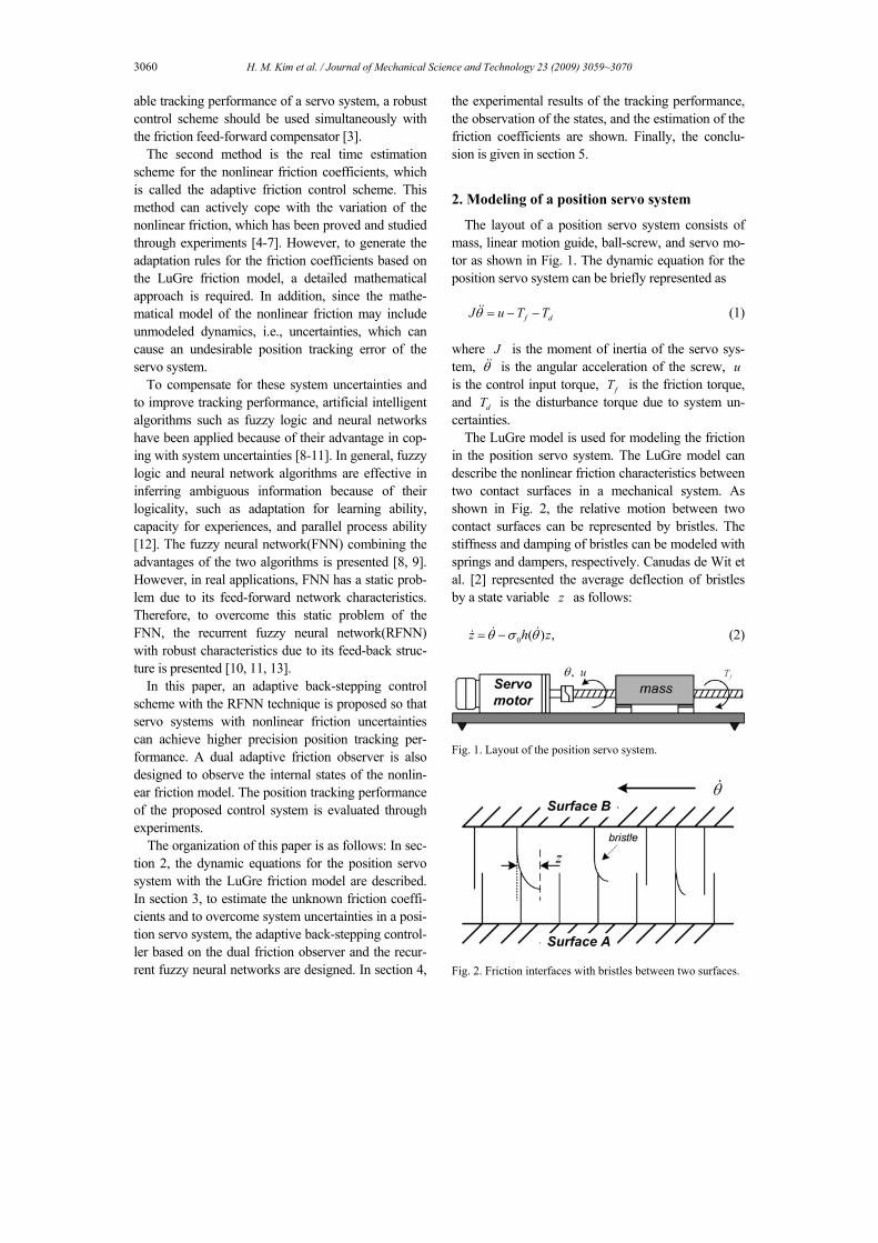
The layout of a position servo system consists of mass, linear motion guide, ball-screw, and servo mo-tor as shown in Fig. 1. The dynamic equation for the position servo system can be briefly represented as

f dJ u T Tθ = − −&& (1)

where J is the moment of inertia of the servo sys-tem, θ&& is the angular acceleration of the screw, u is the control input torque, fT is the friction torque, and dT is the disturbance torque due to system un-certainties.

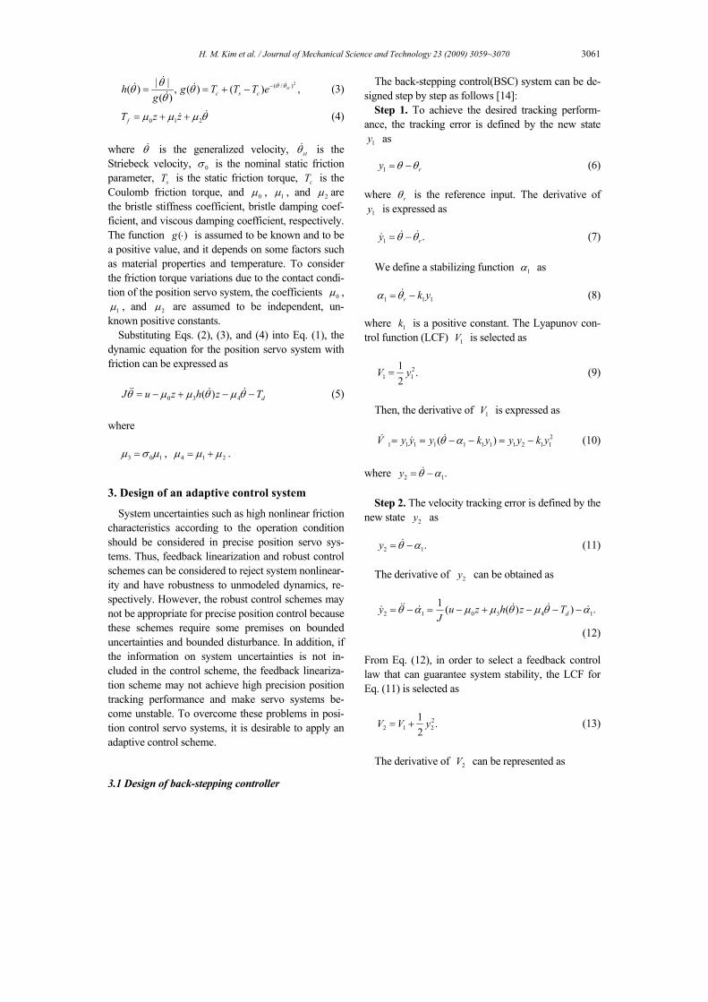
The LuGre model is used for modeling the friction in the position servo system. The LuGre model can describe the nonlinear friction characteristics between two contact surfaces in a mechanical system. As shown in Fig. 2, the relative motion between two contact surfaces can be represented by bristles. The stiffness and damping of bristles can be modeled with springs and dampers, respectively. Canudas de Wit et al. [2] represented the average deflection of bristles by a state variable z as follows:

0 ( ) ,z h zθ σ θ= −& && (2)

Fig. 1. Layout of the position servo system.

Fig. 2. Friction interfaces with bristles between two surfaces.

H. M. Kim et al. / Journal of Mechanical Science and Technology 23 (2009) 3059~3070 3061

2( / )| |( ) , ( ) ( ) ,( )

stc s ch g T T T e

gθ θθθ θ

θ−= = + −

& &&

& &&

(3)

0 1 2fT z zµ µ µ θ= + + && (4)

where θ& is the generalized velocity, stθ& is the Striebeck velocity, 0σ is the nominal static friction parameter, sT is the static friction torque, cT is the Coulomb friction torque, and 0µ , 1µ , and 2µ are the bristle stiffness coefficient, bristle damping coef-ficient, and viscous damping coefficient, respectively. The function ( )g ⋅ is assumed to be known and to be a positive value, and it depends on some factors such as material properties and temperature. To consider the friction torque variations due to the contact condi-tion of the position servo system, the coefficients 0µ ,

1µ , and 2µ are assumed to be independent, un-known positive constants.

Substituting Eqs. (2), (3), and (4) into Eq. (1), the dynamic equation for the position servo system with friction can be expressed as

0 3 4( ) dJ u z h z Tθ µ µ θ µ θ= − + − −&& & & (5)

where

3 0 1µ σ µ= , 4 1 2µ µ µ= + .

3. Design of an adaptive control system

System uncertainties such as high nonlinear friction characteristics according to the operation condition should be considered in precise position servo sys-tems. Thus, feedback linearization and robust control schemes can be considered to reject system nonlinear-ity and have robustness to unmodeled dynamics, re-spectively. However, the robust control schemes may not be appropriate for precise position control because these schemes require some premises on bounded uncertainties and bounded disturbance. In addition, if the information on system uncertainties is not in-cluded in the control scheme, the feedback lineariza-tion scheme may not achieve high precision position tracking performance and make servo systems be-come unstable. To overcome these problems in posi-tion control servo systems, it is desirable to apply an adaptive control scheme.

3.1 Design of back-stepping controller

The back-stepping control(BSC) system can be de-signed step by step as follows [14]:

Step 1. To achieve the desired tracking perform-ance, the tracking error is defined by the new state

1y as

1 ry θ θ= − (6)

where rθ is the reference input. The derivative of 1y is expressed as

1 .ry θ θ= −& && (7)

We define a stabilizing function 1α as

1 1 1r k yα θ= −& (8)

where 1k is a positive constant. The Lyapunov con-trol function (LCF) 1V is selected as

21 1

1 .2

V y= (9)

Then, the derivative of 1V is expressed as

21 1 1 1 1 1 1 1 2 1 1( )V y y y k y y y k yθ α= = − − = −&& & (10)

where 2 1.y θ α= −&

Step 2. The velocity tracking error is defined by the new state 2y as

2 1.y θ α= −& (11)

The derivative of 2y can be obtained as

2 1 0 3 4 11 ( ( ) ) .dy u z h z TJ

θ α µ µ θ µ θ α= − = − + − − −&& & && &&

(12)

From Eq. (12), in order to select a feedback control law that can guarantee system stability, the LCF for Eq. (11) is selected as

22 1 2

1 .2

V V y= + (13)

The derivative of 2V can be represented as

3062 H. M. Kim et al. / Journal of Mechanical Science and Technology 23 (2009) 3059~3070

2 1 2 2

21 1 2 1 0 3 4 1

1[ ( ( ) ) ].d

V V y y

k y y y u z h z TJ

µ µ θ µ θ α

= +

= − + + − + − − −

& & &

& & &

(14) If the last term in Eq. (14) is defined as

1 0 3 4 1 2 21 ( ( ) )dy u z h z T k yJ

µ µ θ µ θ α+ − + − − − = −& & &

(15)

where 2( 0)k > is a design parameter, then the BSC law as the feedback control law can be selected as

1 2 2 1 0 3 4( ) ( ) .du J y k y z h z Tα µ µ θ µ θ= − − + + − + +& && (16)

However, in Eq. (16), the internal state z of the friction model cannot be measured, and friction pa-rameters and the disturbance torque dT cannot be known exactly. In addition, if the friction terms in Eq. (16) cannot be exactly considered in position control servo systems, a large steady-state error may occur.

3.2 Design of adaptive back-stepping controller and

dual friction observer

To select a desired control law, a dual-observer [7] to estimate the unmeasurable internal state z in the friction model is applied as follows:

0 0 0 0ˆ ˆ( ) ,z h zθ σ θ η= − +& & & (17)

1 0 1 1ˆ ˆ( ) ,z h zθ σ θ η= − +& & & (18)

where 0z and 1z are the estimated values of the internal states in the friction model, and 0η and 1η are the observer dynamic terms which can be ob-tained from an adaptive rule. The corresponding ob-servation errors are given by

0 0 0 0( ) ,z h zσ θ η= − −&&% % (19)

1 0 1 1( ) ,z h zσ θ η= − −&&% % (20)

where 0 0ˆz z z= −% and 1 1z z z= −% . Equations (19) and (20) will be induced from the adaptive rule.

To induce the adaptive rule to guarantee stability against unknown parameters and the observer dy-namic terms, the reconstruction error E is defined as

ˆ

d dE T T= − (21)

where dT is the estimated value of dT and it is assumed that E E≤ , where E denotes the bounded value of E .

We now select the 3rd LCF as follows:

23 2

1 ˆ( )2

V V E Eρ

= + − (22)

where ( 0)ρ > is a positive constant and E is the estimated value of the reconstruction error. The de-rivative of 3V can be represented as

3 2

21 1 2 1 0 3

4 1

1 ˆ ˆ( )

1[ ( ( )

1 ˆ ˆ) ] ( )d

V V E E E

k y y y u z h zJ

T E E E

ρ

µ µ θ

µ θ αρ

= + −

= − + + − +

− − − + −

&& &

&

&& &

(23)

From Eq. (23), the adaptive back-stepping con-trol(ABSC) law can be selected as

1 2 2 1 0 0 3 1 4ˆ ˆˆ ˆ ˆˆ ˆ( ) ( ) du J y k y z h z T Eα µ µ θ µ θ= − − + + − + + +& &&

(24)

Substituting Eq. (24) into Eq. (23), then

2 2 23 1 1 2 2 0 0 0 0 3 1

3 1 4

ˆ[ ( )

1ˆ ˆ ˆ ˆˆ( ) ) ] ( )d d

yV k y k y z z h zJ

h z T T E E E E

µ µ µ θ

µ θ µ θρ

= − − + − − +

+ − + − + + −

&& %% %

&& &% %

(25)

where 0 0 0ˆµ µ µ= −% , 3 3 3ˆµ µ µ= −% , and 4 4 4ˆµ µ µ= −% are the unknown parameter estimate errors. The 4th LCF 4V is selected as

2 2 2 2 24 3 0 0 3 1 0 3 4

0 3 4

1 1 1 1 1 .2 2 2 2 2

V V z zµ µ µ µ µγ γ γ

= + + + + +% % %% %

(26) The derivative of 4V can be obtained as

H. M. Kim et al. / Journal of Mechanical Science and Technology 23 (2009) 3059~3070 3063

2 2 2 24 1 1 2 2 0 0 0 3 0 1

2 20 0 0 3 1 3

0 3

2 24 4 0 0 0 0

4

2 21 3 3 1

( ) ( )

1 ( ) 1ˆ ˆˆ ˆ( ) ( )

1 ˆ( ) ( )

1 ˆ( ( ) ) ( ).

V k y k y h z h z

y y hz zJ Jy yzJ Jy yz h E EJ J

µ σ θ µ σ θ

θµ µ µ µγ γ

µ θ µ µ µ ηγ

µ θ µ ηρ

= − − − −

+ − − + −

+ − − + − −

+ − + +

& && % %

&& &% %

&&% %

&& %%

(27)

From Eq. (27), the update laws can be determined as

00 2 0ˆ ˆ ,y z

Jγµ = −& (28)

33 2 1ˆ ˆ( ) ,y h z

Jγµ θ=& & (29)

44 2ˆ ,y

Jγµ θ= −& & (30)

and the observer dynamic terms are expressed as

20 ,y

Jη = − (31)

21 ( ),y h

Jη θ= & (32)

2ˆ .yEJ

ρ= −& (33)

Then, Eq. (27) can be represented as

2 2 24 1 1 2 2 0 0 0

2 2 23 0 1 1 1 2 2

( )

( ) 0.

V k y k y h z

h z k y k y

µ σ θ

µ σ θ

= − − −

− ≤ − − ≤

&& %

& % (34)

From Eq. (34), we can define ( )W y as follows:

1 1 2 2 1 2( ) ( , )W y k y k y V y y= + ≤ − & (35)

Since 0V ≤& , V is a non-increasing function. Thus, it has a limit V∞ as t →∞ . Integrating Eq. (35), then

{ }0 0

1 2

0 0 0 0

lim ( ( )) lim ( , )

lim ( ( ), ) ( ( ), ) ( ( ), )

t t

t tt t

t

W y d V y y d

V y t t V y t t V y t t V

τ τ τ→∞ →∞

∞→∞

≤ −

= − = −

∫ ∫ &

(36)

which means that 0

( ( ))t

tW y dτ τ∫ exists and is finite.

Since ( )W y is also uniformly continuous, the fol-

lowing result can be obtained from the Barbalat lemma [14, 15] as

lim ( ) 0.t

W y→∞

= (37)

Since 1y and 2y are converged to zero as t →∞ , θ and θ& approach to rθ and rθ& , respectively, as t →∞ . Therefore, the ABSC system can be asymp-totically stable in spite of the variation of system pa-rameters and external disturbance.

3.3 Design of recurrent fuzzy neural networks

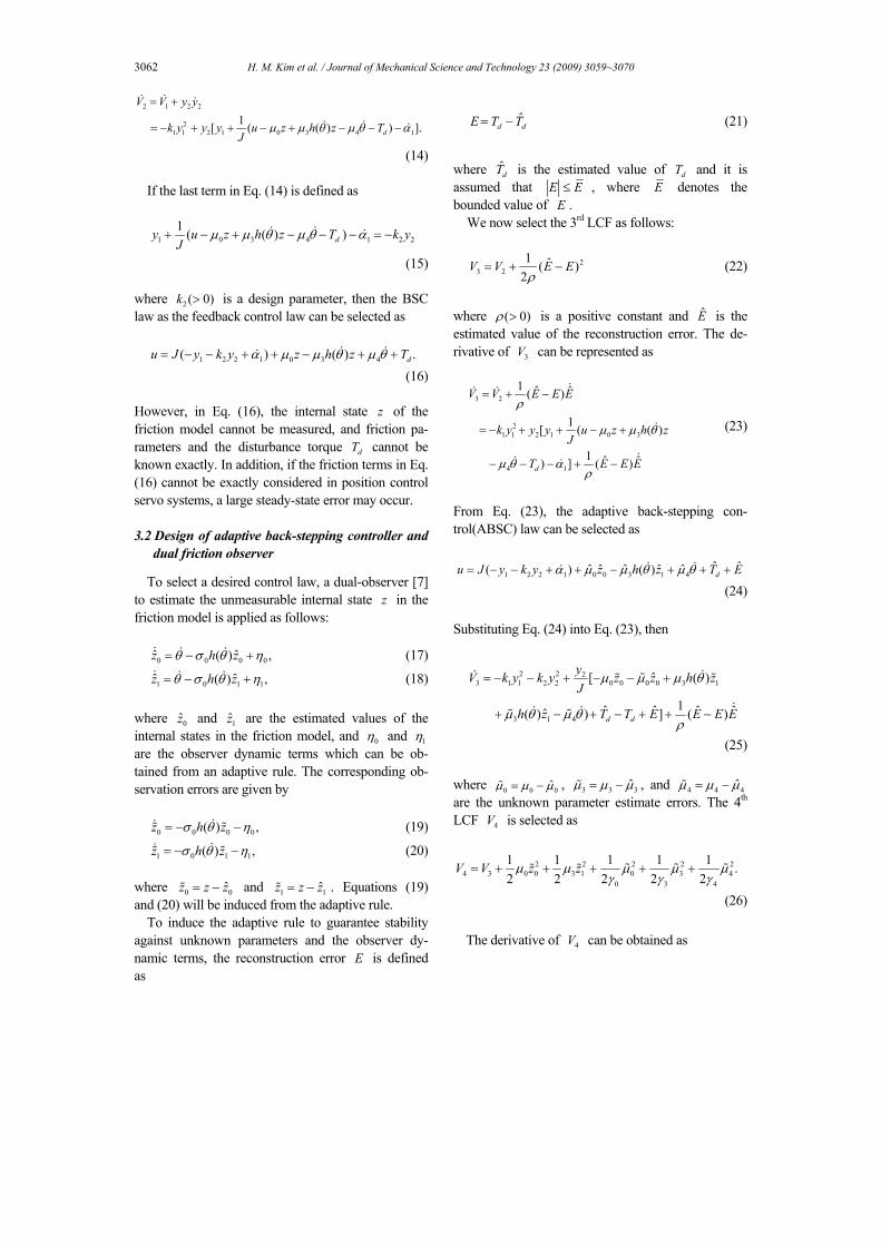
To determine the lumped uncertainty dT , a RFNN observer of a 4-layer structure is proposed, which is shown in Fig. 3. Layer 1 is the input layer with the recurrent loop, which accepts the two input variables. Layer 2 represents the fuzzy rules for calculating the Gaussian membership values. Layer 3 is the rule layer, which represents the preconditions and consequence for the links before and after layer 3, respectively. Layer 4 is the output layer. The interaction and learn-ing algorithms for the layers are given as follows:

A. Description of the RFNN Layer 1, Input layer: For each node i, the net input

and output are represented, respectively, as

1 1 1 1net ( 1),i i i ix w y N= + ⋅ − (38) 1 1 1 1( ) (net ( )) net ( ), 1, 2i i i iy N f N N i= = = (39)

where 1

1 1x y= , 12x y= & , 1

iw is the recurrent weights, and N denotes the number of iterations.

Fig. 3. A general four-layer RFNN.

3064 H. M. Kim et al. / Journal of Mechanical Science and Technology 23 (2009) 3059~3070

Layer 2, Membership layer: For each node, the Gaussian membership values are calculated. For the j th node,

2 2

22

( )net ( )

( )i ij

jij

x mN

σ−

= − (40)

2 2 2 2( ) (net ( )) exp(net ( )), 1,...,j j j jy N f N N j n= = =

(41)

where ijm and ijσ are the mean and standard de-viation of the Gaussian function in the jth term of the ith input linguistic variable 2

ix to the node of layer 2, respectively. n is the total number of the linguistic variables with respect to the input nodes.

Layer 3, Rule layer: Each node k in this layer is de-noted by ∏. In addition, the input signals in this layer are multiplied by each other and then the result of the product is generated. For the kth rule node

3 3 3net ( ) ( ),k jk j

j

N w x N=∏ (42)

3 3 3 3( ) (net ( )) net ( ), 1, ... ,k k k ky N f N N k l= = = (43)

where 3jx represents the jth input to the node of layer

3, 3jkw is the weights between the membership layer

and the rule layer. ( / )il n i= is the number of rules with complete rule connection, if each input node has the same linguistic variables.

Layer 4, Output layer: The single node o in this layer is labeled as Σ , which computes the overall output as the summation of all input signals:

4 4 4net ( ) ( ),o ko k

kN w x N=∑ (44)

4 4 4 4( ) (net ( )) net ( )o o o oy N f N N= = (45)

where the connecting weight 4kow is the output action

strength of the oth output associated with the kth rule. 4kx represents the kth input to the node of layer 4,

and 4 ˆo dy T= .

B. On-line learning algorithm In the learning algorithm, it is important to select

parameters for the membership functions and weights to decide network performance. To train the RFNN effectively, on-line parameter learning is executed by the gradient decent method. There are four adjustable parameters. Our goal is to minimize the error function e represented as

2 21

1 1( ) ( )2 2re yθ θ= − = . (46)

By using the gradient descent method, the weight in each layer is updated as follows:

Layer 4: The weight is updated by an amount

44 4

14 4 4

netnet

oko w w w k

ko o ko

e e uw y xw u w

η η η⎛ ⎞⎛ ⎞∂ ∂ ∂ ∂

∆ = − = − =⎜ ⎟⎜ ⎟∂ ∂ ∂ ∂⎝ ⎠⎝ ⎠

(47)

where 1 4neto

e uyu∂ ∂

= −∂ ∂

and wη is the learning-rate

parameter of the connecting weights of the RFNN. Layer 3: Since the weights in this layer are unified,

the approximated error term needs to be calculated and propagated to calculate the error term of layer 2 as follows:

4 3

3 413 4 3 3

netnet net net

o kk ko

k o k k

e e u y y wu y

δ ∂ ∂ ∂ ∂ ∂= − = − =

∂ ∂ ∂ ∂ ∂ (48)

Layer 2: The multiplication operation is executed

in this layer by using Eq. (46). To update the mean of the Gaussian function, the error term is computed as follows:

24 3 3

22 4 3 3 2 2

3 3

net netnet net net

jo k kj

j o k k j j

k kk

ye e u ynet u y y

y

δ

δ

∂∂ ∂ ∂ ∂ ∂ ∂= − = −

∂ ∂ ∂ ∂ ∂ ∂ ∂

=∑

(49)

and then the update law of ijm is

2 2

2 2

22

2

netnet

2( )

j jij m m

ij j j ij

i ijm j

ij

ye emm y m

x m

η η

η δσ

∂ ∂∂ ∂∆ = − = −

∂ ∂ ∂ ∂

−=

(50)

where mη is the learning-rate parameter of the mean of the Gaussian functions. The update law of ijσ is

2 2

2 2

2 22

3

netnet

2( )

j jij s s

ij j j ij

i ijs j

ij

ye ey

x m

σ η ησ σ

η δσ

∂ ∂∂ ∂∆ = − = −

∂ ∂ ∂ ∂

−=

(51)

H. M. Kim et al. / Journal of Mechanical Science and Technology 23 (2009) 3059~3070 3065

Fig. 4. Photograph of the servo position tracking control system. where sη is the learning-rate parameter of the stan-dard deviation of the Gaussian functions.

The weight, mean, and standard deviation of the hidden layer can be updated by using the following equations:

4 4 4( 1)ko ko kow N w w+ = + ∆ (52) ( 1) ( )ij ij ijm N m N m+ = + ∆ (53) ( 1) ( )ij ij ijN Nσ σ σ+ = + ∆ (54)

4. Experiment results

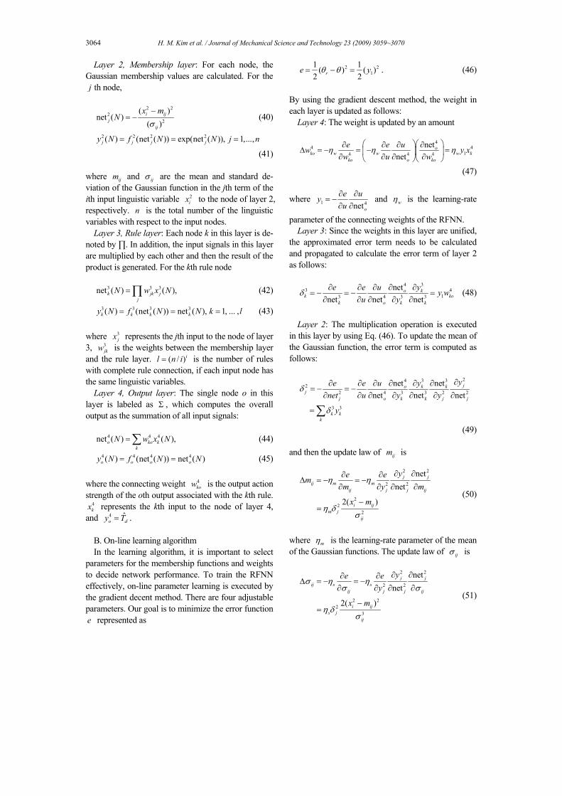
Fig. 4 shows a photograph of the servo position tracking control system to evaluate the performance of control schemes. The angular position was meas-ured with an incremental rotary encoder whose count per encoder was 4 times of 10000 pulses per revolu-tion. A data acquisition board with D/A 12-bit resolu-tion was used to supply the driving voltage to the motor. The sampling rate of the servo system was selected as 500 Hz. The control algorithms were pro-grammed with C-language. The parameters of the servo system and friction model for experiment are shown in Table 1. The block diagram of the ABSC system with RFNN is shown in Fig. 5.

To evaluate the performance of the servo system with the proposed control scheme, two reference in-puts were applied as follows:

1

0.1sin(0.4 )r tθ π= [rad],

20.1sin(0.125 ) sin(0.75 )r t tθ π π= [rad]

To compare the tracking performances of the BSC

system, ABSC system, ABSC system with RFNN, the reference input

1rθ was continuously used for

experiment as follows: the BSC system was applied

Table 1. Parameters of the servo and friction model.

Parameter Notation Value

Moment of inertia J 5 22.3 10 kgm−× Bristles stiffness

coefficient 0σ 0.15 Nm

Stribeck velocity stθ& 0.013 rad/s

Coulomb friction cT 31.97 10 Nm−×

Static friction sT 32.6 10 Nm−×

Fig. 5. Block diagram of the ABSC system with RFNN.

during the initial 20 seconds, the ABSC system dur-ing the 40 seconds after the application of the BSC system, and the ABSC system with RFNN during the 40 seconds after the application of the ABSC system. The reference input

2rθ was independently experi-

mented for the ABSC system and the ABSC system with RFNN, respectively. In addition, the structure of the RFNN is defined to two neurons at inputs of which each has a recurrent loop, five neurons at membership layer, five neurons at rule layer, and one neuron at output layer. The fuzzy sets at the member-ship layer, which have the mean ( ijm ) and standard deviation ( ijσ ), were determined according to the maximum variation boundaries of 1y and 2y of the ABSC system without RFNN. ijm and ijσ vectors applied to experiment are selected as follows:

1 1[ 0.002, 0.001, 0.0, 0.001, 0.002]jm κ= − − × ,

2 2[ 0.2, 0.1, 0.0, 0.1, 0.2]jm κ= − − × ,

1 3[0.003, 0.003, 0.003, 0.003, 0.003]jσ κ= × ,

2 4[0.3, 0.3, 0.3, 0.3, 0.3]jσ κ= × .

where 1 jm and 1 jσ indicate the mean and standard deviation vectors of 1y , respectively, 2 jm and 2 jσ indicate the mean and standard deviation vectors of

2y , respectively, and 1,( 1,2,3,4)i iκ = = . Fig. 6 shows the error of the BSC system, ABSC

system, and ABSC system with RFNN for the refer-ence input

1rθ . The angular displacement rms(root

mean square) error of the BSC system is 0.0054. While the ABSC system is operating, its maximum

3066 H. M. Kim et al. / Journal of Mechanical Science and Technology 23 (2009) 3059~3070

Fig. 6. Error of the BSC system, ABSC system, and ABSC system with RFNN for the reference input

1rθ .

error tends to exponentially decrease and then con-verge to a steady state value due to 0σ , 3σ , and 4σ by the update rules. The angular displacement rms error of the ABSC system is 0.0027. In the operating range of the ABSC system with RFNN, the angular displacement error converges to a steady state value after experiencing a transient state for about 1 second because of the switch from the ABSC system to the ABSC system with RFNN. The angular displacement rms error is 0.0005. The tracking performance of the ABSC system compared with it of the BSC system is improved by 2 times and it of the ABSC system with RFNN compared with it of the ABSC system is im-proved by 5.4 times. The performance improvement of the ABSC system with RFNN implies that the control input of the RFNN including the reconstruc-tion estimation compensates system uncertainties.

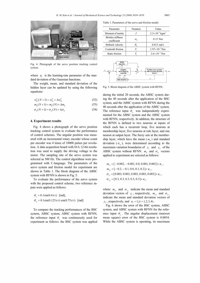
Fig. 7 shows the estimation and the observation of the BSC system, ABSC system, and ABSC system with RFNN for the reference input

1rθ . The estima-

tions by the update rule are shown in Fig. 7(a). The BSC system estimates the friction parameter to be 0, because the BSC system does not have the update rule for 0σ , 3σ , and 4σ . When the ABSC system is applied to the servo system, the update rules estimates the friction parameters, which converge to some val-ues; this convergence stabilizes the servo position system. When the ABSC system is switched to the ABSC system with RFNN, the estimations of the friction parameters do not vary because the angular displacement error is largely decreased by the RFNN. Therefore, the friction estimation values can maintain steady state in the operating range where the RFNN is used. Fig. 7(b) shows the observations of the dual obse rve r . The sp ike pheno menon o f 0z

(a) Estimations of the update rule

(b) 0z and 1z of the dual observer

Fig. 7. Estimation and observation of the BSC system, ABSC system, and ABSC system with RFNN for the reference input

1rθ . among both observation values occurs to a changing point of velocity, because 2y corresponds to the velocity error, which directly affects 0z , as described in Eq. (31). However, in the case of the ABSC system with RFNN, the spike phenomenon of 0z is largely removed, which means that the RFNN compensates system uncertainties such as nonlinear friction includ-ing Coulomb friction, static friction, Stribeck velocity, and unmodeled dynamics.

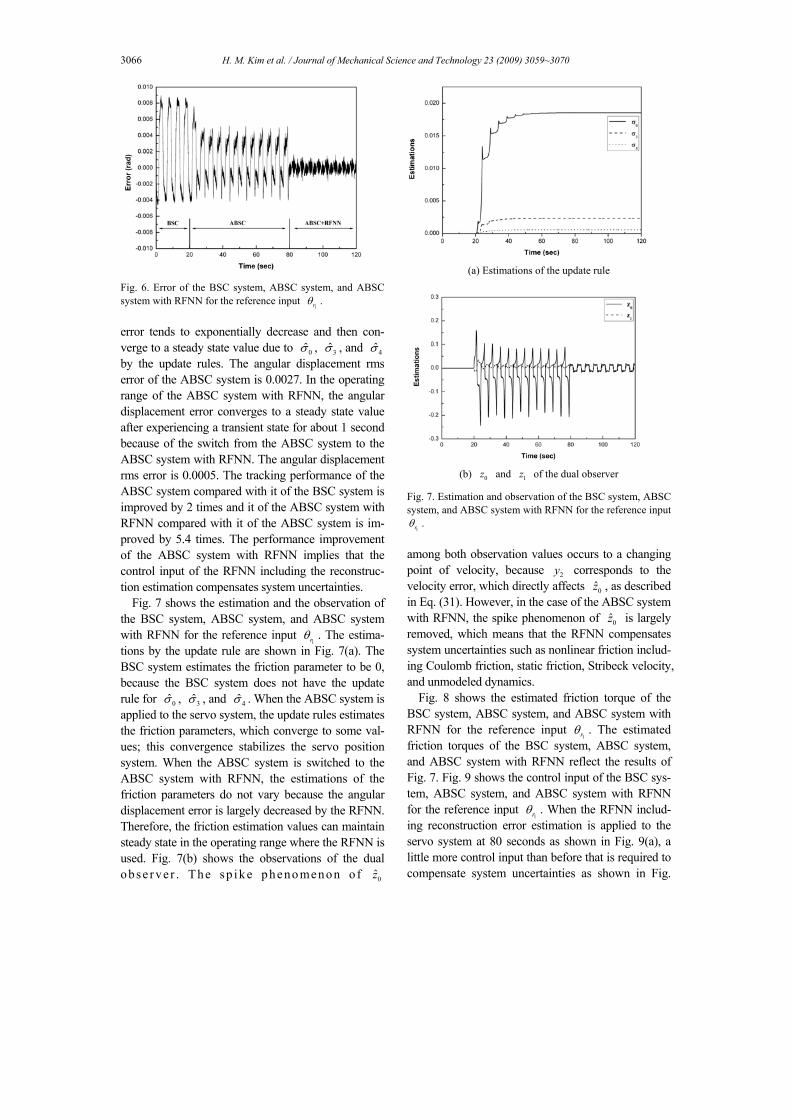
Fig. 8 shows the estimated friction torque of the BSC system, ABSC system, and ABSC system with RFNN for the reference input

1rθ . The estimated

friction torques of the BSC system, ABSC system, and ABSC system with RFNN reflect the results of Fig. 7. Fig. 9 shows the control input of the BSC sys-tem, ABSC system, and ABSC system with RFNN for the reference input

1rθ . When the RFNN includ-

ing reconstruction error estimation is applied to the servo system at 80 seconds as shown in Fig. 9(a), a little more control input than before that is required to compensate system uncertainties as shown in Fig.

H. M. Kim et al. / Journal of Mechanical Science and Technology 23 (2009) 3059~3070 3067

Fig. 8. Estimated friction torque of the BSC system, ABSC system, and ABSC system with RFNN for the reference input

1rθ .

(a) Estimated torque of the RFNN including the reconstruc-

tion error

(b) Control input torque applied to the servo system

Fig. 9. Control inputs of the BSC system, ABSC system, and ABSC system with RFNN for the reference input

1rθ .

9(b). In addition, the deflection of the control input removes the deflection of the error for the BSC and ABSC systems, which is shown in Fig. 6.

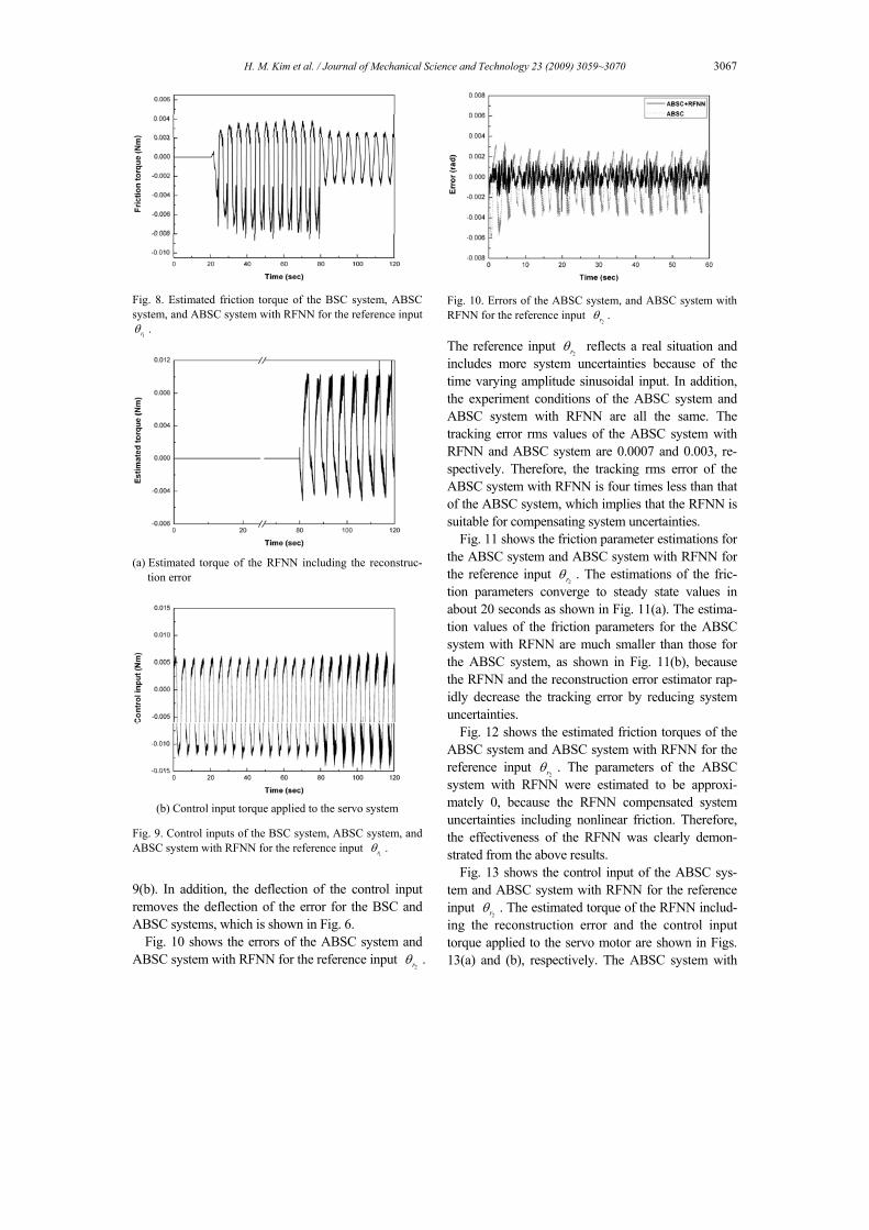
Fig. 10 shows the errors of the ABSC system and ABSC system with RFNN for the reference input

2rθ .

Fig. 10. Errors of the ABSC system, and ABSC system with RFNN for the reference input

2rθ .

The reference input

2rθ reflects a real situation and

includes more system uncertainties because of the time varying amplitude sinusoidal input. In addition, the experiment conditions of the ABSC system and ABSC system with RFNN are all the same. The tracking error rms values of the ABSC system with RFNN and ABSC system are 0.0007 and 0.003, re-spectively. Therefore, the tracking rms error of the ABSC system with RFNN is four times less than that of the ABSC system, which implies that the RFNN is suitable for compensating system uncertainties.

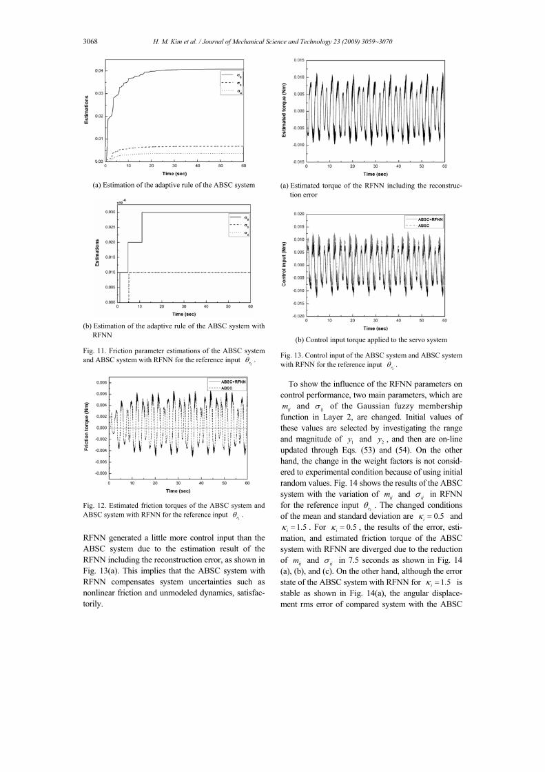
Fig. 11 shows the friction parameter estimations for the ABSC system and ABSC system with RFNN for the reference input

2rθ . The estimations of the fric-

tion parameters converge to steady state values in about 20 seconds as shown in Fig. 11(a). The estima-tion values of the friction parameters for the ABSC system with RFNN are much smaller than those for the ABSC system, as shown in Fig. 11(b), because the RFNN and the reconstruction error estimator rap-idly decrease the tracking error by reducing system uncertainties.

Fig. 12 shows the estimated friction torques of the ABSC system and ABSC system with RFNN for the reference input

2rθ . The parameters of the ABSC

system with RFNN were estimated to be approxi-mately 0, because the RFNN compensated system uncertainties including nonlinear friction. Therefore, the effectiveness of the RFNN was clearly demon-strated from the above results.

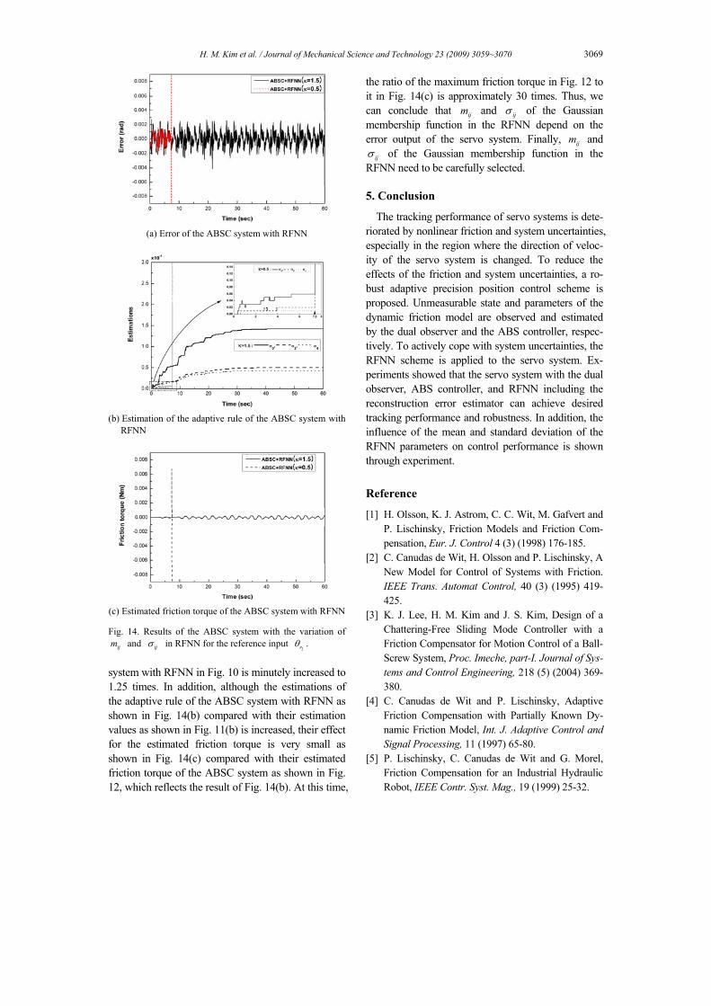
Fig. 13 shows the control input of the ABSC sys-tem and ABSC system with RFNN for the reference input

2rθ . The estimated torque of the RFNN includ-

ing the reconstruction error and the control input torque applied to the servo motor are shown in Figs. 13(a) and (b), respectively. The ABSC system with

3068 H. M. Kim et al. / Journal of Mechanical Science and Technology 23 (2009) 3059~3070

(a) Estimation of the adaptive rule of the ABSC system

(b) Estimation of the adaptive rule of the ABSC system with

RFNN Fig. 11. Friction parameter estimations of the ABSC system and ABSC system with RFNN for the reference input

2rθ .

Fig. 12. Estimated friction torques of the ABSC system and ABSC system with RFNN for the reference input

2rθ .

RFNN generated a little more control input than the ABSC system due to the estimation result of the RFNN including the reconstruction error, as shown in Fig. 13(a). This implies that the ABSC system with RFNN compensates system uncertainties such as nonlinear friction and unmodeled dynamics, satisfac-torily.

(a) Estimated torque of the RFNN including the reconstruc-

tion error

(b) Control input torque applied to the servo system

Fig. 13. Control input of the ABSC system and ABSC system with RFNN for the reference input

2rθ .

To show the influence of the RFNN parameters on

control performance, two main parameters, which are ijm and ijσ of the Gaussian fuzzy membership

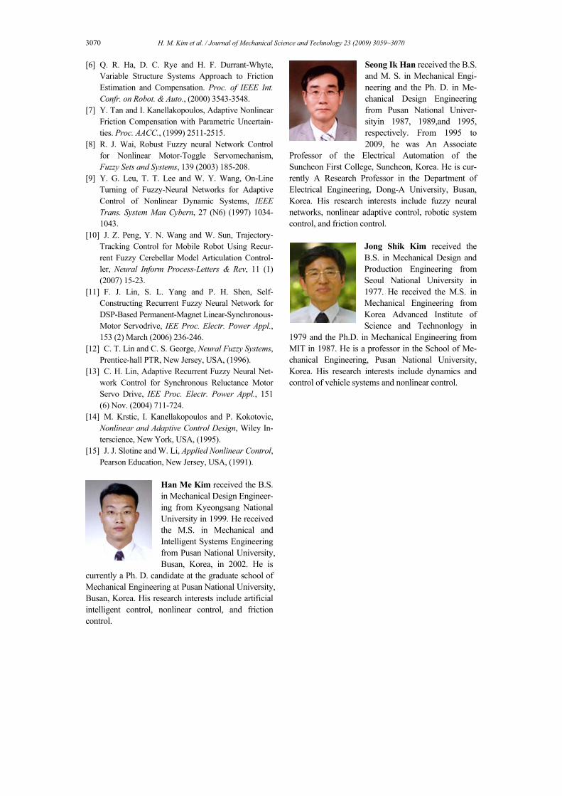
function in Layer 2, are changed. Initial values of these values are selected by investigating the range and magnitude of 1y and 2y , and then are on-line updated through Eqs. (53) and (54). On the other hand, the change in the weight factors is not consid-ered to experimental condition because of using initial random values. Fig. 14 shows the results of the ABSC system with the variation of ijm and ijσ in RFNN for the reference input

2rθ . The changed conditions

of the mean and standard deviation are 0.5iκ = and 1.5iκ = . For 0.5iκ = , the results of the error, esti-

mation, and estimated friction torque of the ABSC system with RFNN are diverged due to the reduction of ijm and ijσ in 7.5 seconds as shown in Fig. 14 (a), (b), and (c). On the other hand, although the error state of the ABSC system with RFNN for 1.5iκ = is stable as shown in Fig. 14(a), the angular displace-ment rms error of compared system with the ABSC

H. M. Kim et al. / Journal of Mechanical Science and Technology 23 (2009) 3059~3070 3069

(a) Error of the ABSC system with RFNN

(b) Estimation of the adaptive rule of the ABSC system with

RFNN

(c) Estimated friction torque of the ABSC system with RFNN Fig. 14. Results of the ABSC system with the variation of

ijm and ijσ in RFNN for the reference input 2r

θ .

system with RFNN in Fig. 10 is minutely increased to 1.25 times. In addition, although the estimations of the adaptive rule of the ABSC system with RFNN as shown in Fig. 14(b) compared with their estimation values as shown in Fig. 11(b) is increased, their effect for the estimated friction torque is very small as shown in Fig. 14(c) compared with their estimated friction torque of the ABSC system as shown in Fig. 12, which reflects the result of Fig. 14(b). At this time,

the ratio of the maximum friction torque in Fig. 12 to it in Fig. 14(c) is approximately 30 times. Thus, we can conclude that ijm and ijσ of the Gaussian membership function in the RFNN depend on the error output of the servo system. Finally, ijm and

ijσ of the Gaussian membership function in the RFNN need to be carefully selected.

5. Conclusion

The tracking performance of servo systems is dete-riorated by nonlinear friction and system uncertainties, especially in the region where the direction of veloc-ity of the servo system is changed. To reduce the effects of the friction and system uncertainties, a ro-bust adaptive precision position control scheme is proposed. Unmeasurable state and parameters of the dynamic friction model are observed and estimated by the dual observer and the ABS controller, respec-tively. To actively cope with system uncertainties, the RFNN scheme is applied to the servo system. Ex-periments showed that the servo system with the dual observer, ABS controller, and RFNN including the reconstruction error estimator can achieve desired tracking performance and robustness. In addition, the influence of the mean and standard deviation of the RFNN parameters on control performance is shown through experiment.

Reference

[1] H. Olsson, K. J. Astrom, C. C. Wit, M. Gafvert and P. Lischinsky, Friction Models and Friction Com-pensation, Eur. J. Control 4 (3) (1998) 176-185.

[2] C. Canudas de Wit, H. Olsson and P. Lischinsky, A New Model for Control of Systems with Friction. IEEE Trans. Automat Control, 40 (3) (1995) 419-425.

[3] K. J. Lee, H. M. Kim and J. S. Kim, Design of a Chattering-Free Sliding Mode Controller with a Friction Compensator for Motion Control of a Ball-Screw System, Proc. Imeche, part-I. Journal of Sys-tems and Control Engineering, 218 (5) (2004) 369-380.

[4] C. Canudas de Wit and P. Lischinsky, Adaptive Friction Compensation with Partially Known Dy-namic Friction Model, Int. J. Adaptive Control and Signal Processing, 11 (1997) 65-80.

[5] P. Lischinsky, C. Canudas de Wit and G. Morel, Friction Compensation for an Industrial Hydraulic Robot, IEEE Contr. Syst. Mag., 19 (1999) 25-32.

3070 H. M. Kim et al. / Journal of Mechanical Science and Technology 23 (2009) 3059~3070

[6] Q. R. Ha, D. C. Rye and H. F. Durrant-Whyte, Variable Structure Systems Approach to Friction Estimation and Compensation. Proc. of IEEE Int. Confr. on Robot. & Auto., (2000) 3543-3548.

[7] Y. Tan and I. Kanellakopoulos, Adaptive Nonlinear Friction Compensation with Parametric Uncertain-ties. Proc. AACC., (1999) 2511-2515.

[8] R. J. Wai, Robust Fuzzy neural Network Control for Nonlinear Motor-Toggle Servomechanism, Fuzzy Sets and Systems, 139 (2003) 185-208.

[9] Y. G. Leu, T. T. Lee and W. Y. Wang, On-Line Turning of Fuzzy-Neural Networks for Adaptive Control of Nonlinear Dynamic Systems, IEEE Trans. System Man Cybern, 27 (N6) (1997) 1034-1043.

[10] J. Z. Peng, Y. N. Wang and W. Sun, Trajectory-Tracking Control for Mobile Robot Using Recur-rent Fuzzy Cerebellar Model Articulation Control-ler, Neural Inform Process-Letters & Rev, 11 (1) (2007) 15-23.

[11] F. J. Lin, S. L. Yang and P. H. Shen, Self-Constructing Recurrent Fuzzy Neural Network for DSP-Based Permanent-Magnet Linear-Synchronous- Motor Servodrive, IEE Proc. Electr. Power Appl., 153 (2) March (2006) 236-246.

[12] C. T. Lin and C. S. George, Neural Fuzzy Systems, Prentice-hall PTR, New Jersey, USA, (1996).

[13] C. H. Lin, Adaptive Recurrent Fuzzy Neural Net-work Control for Synchronous Reluctance Motor Servo Drive, IEE Proc. Electr. Power Appl., 151 (6) Nov. (2004) 711-724.

[14] M. Krstic, I. Kanellakopoulos and P. Kokotovic, Nonlinear and Adaptive Control Design, Wiley In-terscience, New York, USA, (1995).

[15] J. J. Slotine and W. Li, Applied Nonlinear Control, Pearson Education, New Jersey, USA, (1991).

Han Me Kim received the B.S. in Mechanical Design Engineer-ing from Kyeongsang National University in 1999. He received the M.S. in Mechanical and Intelligent Systems Engineering from Pusan National University, Busan, Korea, in 2002. He is

currently a Ph. D. candidate at the graduate school of Mechanical Engineering at Pusan National University, Busan, Korea. His research interests include artificial intelligent control, nonlinear control, and friction control.

Seong Ik Han received the B.S. and M. S. in Mechanical Engi-neering and the Ph. D. in Me-chanical Design Engineering from Pusan National Univer-sityin 1987, 1989,and 1995, respectively. From 1995 to 2009, he was An Associate

Professor of the Electrical Automation of the Suncheon First College, Suncheon, Korea. He is cur-rently A Research Professor in the Department of Electrical Engineering, Dong-A University, Busan, Korea. His research interests include fuzzy neural networks, nonlinear adaptive control, robotic system control, and friction control.

Jong Shik Kim received the B.S. in Mechanical Design and Production Engineering from Seoul National University in 1977. He received the M.S. in Mechanical Engineering from Korea Advanced Institute of Science and Technonlogy in

1979 and the Ph.D. in Mechanical Engineering from MIT in 1987. He is a professor in the School of Me-chanical Engineering, Pusan National University, Korea. His research interests include dynamics and control of vehicle systems and nonlinear control.