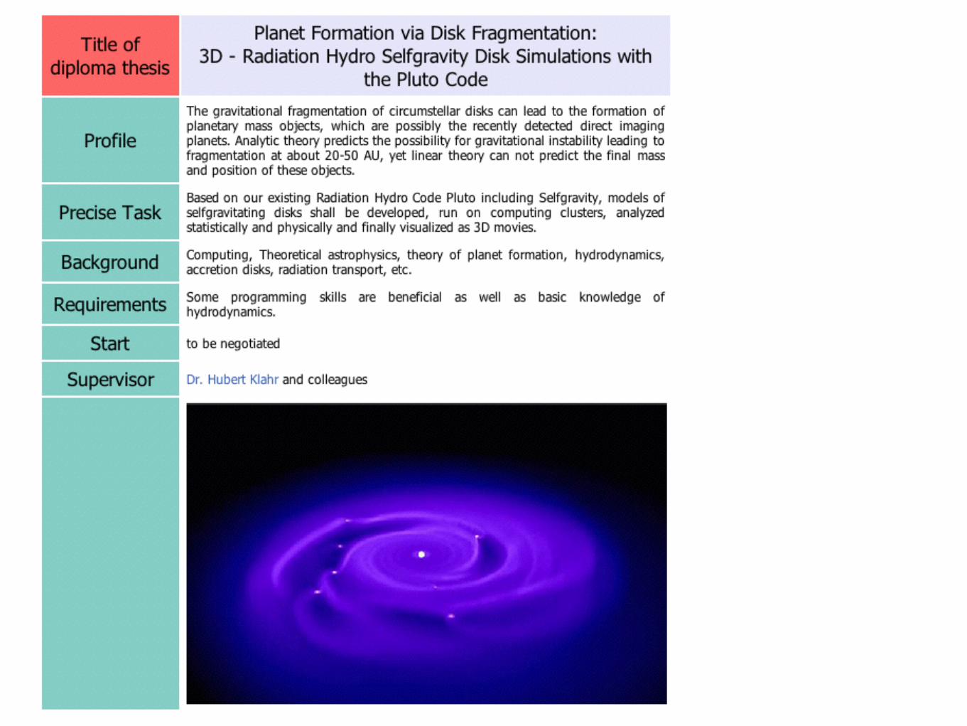
Practical Numerical Training UKNumConclusions

Dr. H. Klahr & Dr. C. Mordasini

Max Planck Institute for Astronomy, Heidelberg

Programm: 1) Weiterführende Vorlesungen 2) Fragebogen 3) Eigene Forschung 4) Bachelor/Masterarbeiten

1 Weitereführende Vorlesungen

2 Fragebogen

3 Eigene Forschung

Galaxies, stars and planets

10 billion galaxies

100 billion stars

how many planets?

How many harbor life?

How frequent? Life? First generation of human beings with technology to answer this.

Sun Stars

Herschel’s 1789

For many centuries

Solar System Exoplanets

La Silla Obs. ESO

For a decade

Cloud collapse Hertzsprung Russel Nuclear Fusion Stellar Mass Funct.

Formation in disks Collisions Gas accretion Migration

Life Extraterrestrial Life ?

Darwin ESA

In a decade ?

Astrobiology Habitable Zone Biomarkers Complex Life

Ways to understanding

Core

Accretion

Gravitational

Instability

Planet formation: The paradigm

- remote observations - in-situ measurements - sample returns - laboratory analysis - theoretical modeling

Party line

A satisfactory theory should explain the formation of planets in the solar system as well as around other stars.

Minority line

dust

planetesimals protoplanets

in presence of gas in absence of gas

giant impacts

terrestrial planets

107 years

giant planets

Star

& p

roto

plan

etar

y di

sk

migration

type I type II

107 years

108 years

dynamical re- arrangement

Planet formation: Sequential picture

• Huge dynamical range in size/mass: grains to giant planets • Multiple input physics: gravity, hydrodynamics, radiative transport,

thermodynamics, magnetic fields, impact physics, material properties, ... • Strong non-linear mechanisms (e.g. runaway growth) • Feedbacks and interactions (e.g. protoplanetary disk-planet: orbital migration)

Quantitatively, planet formation is a complex process

Planet formation and evolution difficult to understand from first principles alone.

Y. Alibert et al.: Giant planet formation 345

The boundary conditions for this part of the calculation arethe same as in PT99, formally,

T (z = H) = T (τab, Tb, r, Mst,α), (4)

P(z = H) =Ω2Hτab

κ(T (z = H), P(z = H)), (5)

F(z = H) =3

8πMstΩ

2, (6)

and

F(z = 0) = 0. (7)

These conditions depend on three parameters: τab the opticaldepth between the surface of the disc (z = H) and infinity,Tb the background temperature, and Mst the equilibrium accre-tion rate defined by Mst ≡ 3πνΣ where Σ ≡

∫ H

−Hρdz is the usual

surface density, and ν ≡∫ H

−H νρdz/Σ. The values for τab andTb are the same as in PT99 (namely 10−2 and 10 K); the steady-state accretion rate is a free parameter. As shown in PT99, thestructure obtained hardly varies with the first two parameters.

This system of 3 equations with 4 boundary conditions hasin general no solution, except for a certain value of H. Thisvalue is found iteratively: Eqs. (1)–(3) are numerically inte-grated from z = H to z = 0, using a fifth-order Runge-Kuttamethod with adaptive step length (Press et al. 1992) untilF(z = 0) = 0 to a given accuracy.

Using this procedure, we calculate, for each distance to thestar r and each value of the equilibrium accretion rate Mst, thedistributions of pressure, temperature and density T (z; r, Mst),P(z; r, Mst), ρ(z; r, Mst).

Using these distributions, we finally calculate the mid-plane temperature (Tmid) and pressure (Pmid), as well asthe effective viscosity ν(r, Mst), the disc density scale heightH(r, Mst) defined by ρ(z = H) = e−1/2ρ(z = 0). The surfacedensity Σ(r, Mst) is also given as a function of Mst (for eachradius). By inverting this former relation, we finally obtain re-lations Tmid(r,Σ), Pmid(r,Σ), ν(r,Σ) and H(r,Σ) for each valueof r (and each value of the other parameters α, τab and Tb).

2.1.2. Evolution of the surface density

The time evolution of the disc is governed by the well-knowndiffusion equation (Lynden-Bell & Pringle 1974):

dΣdt=

3r∂

∂r

[r1/2 ∂

∂r(νΣr1/2)

]=

1r∂

∂r(rJ(r)) , (8)

where J(r) ≡ 3r1/2

∂∂r (νΣr1/2) is the mass flux (integrated over the

vertical axis z). This equation is modified to take into accountthe momentum transfer between the planet and the disc, as wellas the effect of photo-evaporation and accretion onto the planet:

dΣdt=

3r∂

∂r

[r1/2 ∂

∂rνΣr1/2 + Λ(r)

]+ Σw(r) + Qplanet(r). (9)

The rate of momentum transfer Λ between the planet andthe disc is calculated using the formula derived by Lin &Papaloizou (1986):

Λ(r) =fΛ2r

√GMstar

(Mplanet

Mstar

)2 ( r

max(|r − a|, H)

)4, (10)

where a is the sun-planet distance and fΛ is a numerical con-stant1. The photo-evaporation term Σw is given by (Veras &Armitage 2004):Σw = 0 for R < Rg,Σw ∝ R−1 for R > Rg,

(11)

where Rg is usually taken to be 5 AU, and the total mass lossdue to photo-evaporation is a free parameter. Finally, a sinkterm Qplanet is included in Eq. (9), to take into account theamount of gas accreted by the planet. This term is generallynegligible compared to the other ones, except during the run-away phases.

To solve the diffusion Eq. (9) we need to specify twoboundary conditions. The first one is given at the outer radiusof the disc (in our simulations this radius is usually taken at50 AU). At this radius, one can either give the surface densityΣ or its temporal derivative. Since the characteristic evolutiontime of the disc is the diffusion timescale

Tν ∝r2

ν∝ 1αΩ

( rH

)2, (12)

which2 is proportional to r3/2 for discs of approximately con-stant aspect ratio (which is the case in these models, see PT99)the outer boundary condition has little influence.

The second condition is specified at the inner radius wherewe have used the following condition:

r∂νΣ

∂r

∣∣∣∣∣∣inner radius

= 0. (13)

Since the total mass flux through a cylinder of radius r is givenby:

Φ(r) ≡ 2πrJ(r) = 3πνΣ + 6πr∂νΣ

∂r, (14)

the boundary condition Eq. (13) can be expressed as:

Φ(r)∣∣∣∣inner radius

= 3πνΣ = Mst, (15)

i.e. the mass flux through the inner radius is equal to the equi-librium flux. Therefore, this condition is equivalent to say thatthe inner disc instantaneously adapt itself to the conditionsgiven by the outer disc. As discussed in PT99, this is consistentwith the expression of the characteristic timescale as a functionof the radius (Eq. (12)).

2.2. Migration rate

Dynamical tidal interactions of the growing protoplanet withthe disc lead to two phenomena: inward migration and gapformation (Lin & Papaloizou 1979, Ward 1997, Tanaka et al.2002). For low mass planets, the tidal interaction is linear, and

1 In this formula, the disc scale height H is the scale height of theunperturbed disc, and not the scale height in the middle of the gap.

2 The second part of Eq. (12) is obtained by expressing Eq. (1) as1ρ

PH ∼ Ω2H and then replacing the sound velocity by ΩH in the defi-

nition of ν.

Y. Alibert et al.: Giant planet formation 345

The boundary conditions for this part of the calculation arethe same as in PT99, formally,

T (z = H) = T (τab, Tb, r, Mst,α), (4)

P(z = H) =Ω2Hτab

κ(T (z = H), P(z = H)), (5)

F(z = H) =3

8πMstΩ

2, (6)

and

F(z = 0) = 0. (7)

These conditions depend on three parameters: τab the opticaldepth between the surface of the disc (z = H) and infinity,Tb the background temperature, and Mst the equilibrium accre-tion rate defined by Mst ≡ 3πνΣ where Σ ≡

∫ H

−Hρdz is the usual

surface density, and ν ≡∫ H

−H νρdz/Σ. The values for τab andTb are the same as in PT99 (namely 10−2 and 10 K); the steady-state accretion rate is a free parameter. As shown in PT99, thestructure obtained hardly varies with the first two parameters.

This system of 3 equations with 4 boundary conditions hasin general no solution, except for a certain value of H. Thisvalue is found iteratively: Eqs. (1)–(3) are numerically inte-grated from z = H to z = 0, using a fifth-order Runge-Kuttamethod with adaptive step length (Press et al. 1992) untilF(z = 0) = 0 to a given accuracy.

Using this procedure, we calculate, for each distance to thestar r and each value of the equilibrium accretion rate Mst, thedistributions of pressure, temperature and density T (z; r, Mst),P(z; r, Mst), ρ(z; r, Mst).

Using these distributions, we finally calculate the mid-plane temperature (Tmid) and pressure (Pmid), as well asthe effective viscosity ν(r, Mst), the disc density scale heightH(r, Mst) defined by ρ(z = H) = e−1/2ρ(z = 0). The surfacedensity Σ(r, Mst) is also given as a function of Mst (for eachradius). By inverting this former relation, we finally obtain re-lations Tmid(r,Σ), Pmid(r,Σ), ν(r,Σ) and H(r,Σ) for each valueof r (and each value of the other parameters α, τab and Tb).

2.1.2. Evolution of the surface density

The time evolution of the disc is governed by the well-knowndiffusion equation (Lynden-Bell & Pringle 1974):

dΣdt=

3r∂

∂r

[r1/2 ∂

∂r(νΣr1/2)

]=

1r∂

∂r(rJ(r)) , (8)

where J(r) ≡ 3r1/2

∂∂r (νΣr1/2) is the mass flux (integrated over the

vertical axis z). This equation is modified to take into accountthe momentum transfer between the planet and the disc, as wellas the effect of photo-evaporation and accretion onto the planet:

dΣdt=

3r∂

∂r

[r1/2 ∂

∂rνΣr1/2 + Λ(r)

]+ Σw(r) + Qplanet(r). (9)

The rate of momentum transfer Λ between the planet andthe disc is calculated using the formula derived by Lin &Papaloizou (1986):

Λ(r) =fΛ2r

√GMstar

(Mplanet

Mstar

)2 ( r

max(|r − a|, H)

)4, (10)

where a is the sun-planet distance and fΛ is a numerical con-stant1. The photo-evaporation term Σw is given by (Veras &Armitage 2004):Σw = 0 for R < Rg,Σw ∝ R−1 for R > Rg,

(11)

where Rg is usually taken to be 5 AU, and the total mass lossdue to photo-evaporation is a free parameter. Finally, a sinkterm Qplanet is included in Eq. (9), to take into account theamount of gas accreted by the planet. This term is generallynegligible compared to the other ones, except during the run-away phases.

To solve the diffusion Eq. (9) we need to specify twoboundary conditions. The first one is given at the outer radiusof the disc (in our simulations this radius is usually taken at50 AU). At this radius, one can either give the surface densityΣ or its temporal derivative. Since the characteristic evolutiontime of the disc is the diffusion timescale

Tν ∝r2

ν∝ 1αΩ

( rH

)2, (12)

which2 is proportional to r3/2 for discs of approximately con-stant aspect ratio (which is the case in these models, see PT99)the outer boundary condition has little influence.

The second condition is specified at the inner radius wherewe have used the following condition:

r∂νΣ

∂r

∣∣∣∣∣∣inner radius

= 0. (13)

Since the total mass flux through a cylinder of radius r is givenby:

Φ(r) ≡ 2πrJ(r) = 3πνΣ + 6πr∂νΣ

∂r, (14)

the boundary condition Eq. (13) can be expressed as:

Φ(r)∣∣∣∣inner radius

= 3πνΣ = Mst, (15)

i.e. the mass flux through the inner radius is equal to the equi-librium flux. Therefore, this condition is equivalent to say thatthe inner disc instantaneously adapt itself to the conditionsgiven by the outer disc. As discussed in PT99, this is consistentwith the expression of the characteristic timescale as a functionof the radius (Eq. (12)).

2.2. Migration rate

Dynamical tidal interactions of the growing protoplanet withthe disc lead to two phenomena: inward migration and gapformation (Lin & Papaloizou 1979, Ward 1997, Tanaka et al.2002). For low mass planets, the tidal interaction is linear, and

1 In this formula, the disc scale height H is the scale height of theunperturbed disc, and not the scale height in the middle of the gap.

2 The second part of Eq. (12) is obtained by expressing Eq. (1) as1ρ

PH ∼ Ω2H and then replacing the sound velocity by ΩH in the defi-

nition of ν.

dP

dt= (3M)1/3

6a2BLM1/3

dMZ

dt

dMZ

dt= pR2

captFG(e, i)

4 Mordasini et al.

BP86; Guillot 2005; Broeg 2010):

dmdr = 4πr2ρ dP

dr = −Gmr2 ρ

dldr = 4πr2ρ

(

ϵ − T ∂S∂t

)

dTdr = T

PdPdr ∇

(2)

In these equations, r is the radius as measured from the planetary cen-ter, m the mass inside r (including the core mass MZ), l the luminosityat r, ρ, P, T, S the gas density, pressure, temperature and entropy, t thetime, and ∇ is given as

∇ = d ln Td lnP = min(∇ad,∇rad) ∇rad = 3

64πσGκlPT 4m (3)

i.e. by the minimum of the adiabatic gradient ∇ad which is directlygiven by the equation of state (in convective zones) or the radiativegradient ∇rad (in radiative zones) where κ is the opacity and σ is theStefan-Boltzmann constant.

Calculation of the luminosity

For the planetary population synthesis, where the evolution of thou-sands of different planets is calculated, we need a stable and rapidmethod for the numerical solution of these equations. We have there-fore replaced the ordinary equation for dl/dr by the assumption thatl is constant within the envelope, and that we can derive the total lu-minosity L (including solid and gas accretion, contraction and releaseof internal heat) and its temporal evolution by total energy conserva-tion arguments, an approach somewhat similar to Papaloizou & Nelson(2005). We first recall that −dEtot/dt = L and that in the hydrostaticcase, the total energy is given as

Etot = Egrav + Eint = −

∫ M

0

Gm

rdm +

∫ M

0u dm = − ξ

GM2

2R(4)

where u is the specific internal energy, M the total mass, and R thetotal radius of the planet. We have defined a parameter ξ, which repre-sents the distribution of mass within the planet and its internal energycontent. The ξ can be found for any given structure at time t with theequations above. Then one can write

− ddtEtot = L = LM + LR + Lξ = ξGM

R M −ξGM2

2R2 R + GM2

2R ξ (5)

where M = MZ + MXY is the total accretion rate of solids and gas, andR is the rate of change of the total radius. All quantities except ξ canreadily be calculated at time t. We now set

L ≃ C (LM + LR) . (6)

4 Mordasini et al.

BP86; Guillot 2005; Broeg 2010):

dmdr = 4πr2ρ dP

dr = −Gmr2 ρ

dldr = 4πr2ρ

(

ϵ − T ∂S∂t

)

dTdr = T

PdPdr ∇

(2)

In these equations, r is the radius as measured from the planetary cen-ter, m the mass inside r (including the core mass MZ), l the luminosityat r, ρ, P, T, S the gas density, pressure, temperature and entropy, t thetime, and ∇ is given as

∇ = d ln Td lnP = min(∇ad,∇rad) ∇rad = 3

64πσGκlPT 4m (3)

i.e. by the minimum of the adiabatic gradient ∇ad which is directlygiven by the equation of state (in convective zones) or the radiativegradient ∇rad (in radiative zones) where κ is the opacity and σ is theStefan-Boltzmann constant.

Calculation of the luminosity

For the planetary population synthesis, where the evolution of thou-sands of different planets is calculated, we need a stable and rapidmethod for the numerical solution of these equations. We have there-fore replaced the ordinary equation for dl/dr by the assumption thatl is constant within the envelope, and that we can derive the total lu-minosity L (including solid and gas accretion, contraction and releaseof internal heat) and its temporal evolution by total energy conserva-tion arguments, an approach somewhat similar to Papaloizou & Nelson(2005). We first recall that −dEtot/dt = L and that in the hydrostaticcase, the total energy is given as

Etot = Egrav + Eint = −

∫ M

0

Gm

rdm +

∫ M

0u dm = − ξ

GM2

2R(4)

where u is the specific internal energy, M the total mass, and R thetotal radius of the planet. We have defined a parameter ξ, which repre-sents the distribution of mass within the planet and its internal energycontent. The ξ can be found for any given structure at time t with theequations above. Then one can write

− ddtEtot = L = LM + LR + Lξ = ξGM

R M −ξGM2

2R2 R + GM2

2R ξ (5)

where M = MZ + MXY is the total accretion rate of solids and gas, andR is the rate of change of the total radius. All quantities except ξ canreadily be calculated at time t. We now set

L ≃ C (LM + LR) . (6)

0 = q

h

22

pr2p

2p

drp

dt= 2r

p

tot

Jp

rH = rp

Mp

3M

1/3

H

1330 A. Crida and A. Morbidelli

6 M O D E L L I N G T H E M I G R AT I O N R AT E

It seems quite logical that, when the planet opens a clean gap, itsmigration follows a proper type II regime. With a Jupiter mass planetand a disc aspect ratio of 0.05, this happens for R > 105 (see Figs 1and 2).

However, for smaller Reynolds numbers, the gap is not com-pletely gasproof. The gas in the gap has two major consequences:(i) it partially sustains the outer disc, effectively reducing the torquefelt by the planet from the outer disc; (ii) it exerts a corotation torqueon to the planet. The possibility of gas flowing through the gap de-couples the planet from the gas evolution.

In this section we show with a simple model that taking intoaccount these effects allows us to explain the evolution of the planetas a function of the various parameters. Our model is based onprevious works on the corotation torque (Masset 2001), the viscousevolution of accretion discs (LP74) and the shape of gaps (Cridaet al. 2006).

6.1 Classical type II torque

In an accretion disc, the viscous stress is such that angular momen-tum flows outward while matter falls on to the star. In a Keplerian,circular disc with ν and " independent of the radius, the torqueexerted by the part of the disc extending from a given radius r0 toinfinity on the inner part r < r0 is Tν = −3π"νr0

2#0 (it canbe easily found from the strain tensor). It causes a mass flow ofgas F, carrying the equivalent angular momentum: Tν = Fr0

2#0 =(2πr0"vr) r0

2#0, where vr is the radial velocity of the gas. In thismodel vr = −(3/2)(ν/r0), which can also be found from the Navier–Stokes equations. This gives the following equality, which we willuse further:

ν = −2vr

3r0. (5)

If a planet opens a deep gap in such a disc, no gas flow is allowedthrough the planetary orbit. The outer disc is maintained outsideof the gap by the planet, and an equilibrium is reached so that theplanetary torque balances Tν . Consequently, the planet feels fromthe outer disc the torque Tν . This torque is proportional to the vis-cosity and not to the planet mass. This is the case of standard typeII migration.

In a more realistic, viscously evolving disc, the scheme for typeII migration is the same, but the above formula for Tν is no longervalid. In that case, the equations of LP74 provide the density, theviscous torque and the radial velocity as a function of radius andtime. In our case of a disc with Rinf > 0, it gives

Tν = 3πν"0T −5/4 (h − hinf) exp

(−ar 2

T

), (6)

"LP74 = Tν

3πν√

r, (7)

F = −∂Tν

∂h, (8)

vr = F2πr"LP74

, (9)

where h = r 2# =√

r is the specific angular momentum. Noticethat equation (6) is exactly equation (25) in LP74, while equation (7)is equivalent to equation (2).

Thus, in standard type II migration, we consider that the planetfeels from the disc a torque

TII = Fh = 2πr+"LP74(r+)vr(r+)√

r+, (10)

where r+ = rp + xs is the radius of the external edge of the gap, and"LP74 and vr come from equations (7) and (9), respectively.

6.2 Torque exerted on the outer disc by the gas in the gap

The gas in the gap, the density of which is denoted "gap, exerts on theouter disc a positive viscous torque T(i) that is given by equation (10),with "gap instead of "LP74 and the opposite sign. This torque par-tially sustains the outer disc, and therefore needs to be subtractedfrom the torque that the planet would suffer from the outer disc ifthe gap were clean (given by equation 10). So, denoting by f theratio "gap/"LP74 we have

T(i) = − f TII. (11)

We now discuss how to evaluate f in practice. We have presentedin Section 5 a way to compute semi-analytically the gap profile andthe gap depth. However, making a step-by-step integration until thebottom of the gap it is not very convenient. Consequently, we lookedfor a simple empirical formula for the gap depth as a function ofthe viscosity, the aspect ratio of the disc and the planet mass. Cridaet al. (2006) showed that the density inside the gap is less than10 per cent of the unperturbed value (i.e. f < 0.1) if and only if

P = 34

HRH

+ 50qR

! 1. (12)

Using equation (3), we have computed the depth of the gap forvarious values of the parameter P . For each value of P , we imposeq = 10−3 and H/r = 0.05, and find the corresponding viscosity.Then, we use these parameters in equation (3); the obtained gapdepth is shown as big dots in Fig. 8. We repeat the same operationfor q ranging from 5 × 10−4 to 2 × 10−3; the results are reportedas crosses in Fig. 8. Furthermore, we impose q = 10−3 and ν =0, and find the corresponding H/r and the resulting gap depth. We

0

0.2

0.4

0.6

0.8

1

1 10

ratio

of t

he g

ap s

urfa

ce d

ensi

ty to

the

unpe

rturb

ed s

urfa

ce d

ensi

ty

P

f(P)q = 0.001H/r = 0.05

H/r = 0.05 ; q = 0.001

Figure 8. Gap depth (measured as ratio of the gap surface density to theunperturbed density at r = rp + 2RH) as a function of P . The data points foreach value of P are obtained from the integration of equation (3), assumingdifferent values of ν and H/r and keeping q = 10−3 (points) or differentvalues of ν and q and keeping H/r = 0.05 (crosses); the big dots correspondto the gap depths obtained for different values of ν and keeping both H/r= 0.05 and q = 10−3 (see text for a more precise description of the sets ofmeasures). The bold line is an approximate fit of the data.

C⃝ 2007 The Authors. Journal compilation C⃝ 2007 RAS, MNRAS 377, 1324–1336

16

Material ρ0 [kg m−3] c [kg m−3 Pa−n] nFe(α) 8300.00 0.00349 0.528MgSiO3 (perovskite) 4100.00 0.00161 0.541(Mg,Fe)SiO3 4260.00 0.00127 0.549H2O 1460.00 0.00311 0.513C (graphite) 2250.00 0.00350 0.514SiC 3220.00 0.00172 0.537

Table 3

Fits to the merged Vinet/BME and TFD EOS of the form ρ(P ) = ρ0 + cP n. These fits are valid for the pressurerange P < 1016 Pa.

Magnetohydrodynamic disk models around young stars

Instabilities in disks

Orbital migration of planets

High mass star formation models

Exoplanets: statistical tests for theoryM

ass

[Ear

th m

ass]

40 III. Selected Research Areas

Since hot Jupiters are much more easily detected by both the radial velocity and the transit method relative to low-mass (respectively small) planets, their number is still lower in Fig. III.1.1, which is not corrected for the observational biases. Two statistical distributions which are linked to the a – M diagram are the semimajor axis distribution and the planetary mass function, which is studied below.

The right panel shows the radius of the extrasolar planets and the planets of the Solar System as a function of mass. The most recent breakthrough in the observa-tion of exoplanets is that it has become possible to not only detect exoplanets, but also to start characterizing them. In this context, the planetary mass-radius diagram is probably the most central representation. The impor-tance of the M– R plot stems from its information con-tent about the inner bulk composition of planets which is the first, very basic geophysical characterization of a planet. In the Solar System, we have three fundamental types of planets, namely terrestrial, gas giant and ice gi-ant planets. The imprint of the bulk composition on the radius is indicated by theoretical lines. Two lines show the theoretical mass-radius relationship for solid planets made of silicates and iron, and of water, while the third line shows the M – R for giant planets consisting most-ly of H/He. Being able to understand and reproduce in a model this second fundamental figure is another goal of planetary population synthesis. The reason for the im-portance for formation theory stems from the fact that it contains additional constraints on the formation process, which we cannot derive from the mass-distance diagram

alone. An example are the observational constraints coming from the M – R diagram on the extent of orbital migration. Efficient inward migration brings ice-dom-inated, low-density planets from the outer parts of the disk close to the star. These planets can be distinguished from planets consisting only of silicates and iron, which have presumably formed in situ in the inner, hotter parts of the disk. In future, the atmospheric composition of exoplanets as measured by, e.g., the planned EChO mis-sion will provide additional, important constraints.

Another important goal of population synthesis that goes beyond the purely planetary properties is to under-stand the correlations between planetary and host star properties.

Population synthesis method

The general framework for population synthesis calcu-lations is shown in Fig. III.1.2. With this framework, theoretical formation models can be tested how far they can reproduce the statistical properties of the en-tire known population. The most important ingredient is the planet formation and evolution model which estab-lishes the link between disk and planetary properties. It will be addressed below. The second central ingredients are sets of initial conditions. These sets are drawn in a Monte Carlo way from probability distributions. These probability distributions represent the different proper-ties of protoplanetary disks and are derived as closely as possible from observational results regarding the

Venus

Earth

UranusNeptune

Saturn

Jupiter

Radial velocity& TransitsMicrolensingDirect imaging

10–2 0,1 1

Mas

s [M

!]

1

10

102

103

104

Rad

ius

[REa

rth]

0

5

10

15

20

10 102 1 10 102

Semimajor axis [AU] Mass [Earth masses]103 104

rocky

ice

jovian

Venus

Neptune

Uranus

Earth

Saturn

Jupiter

Fig. III.1.1: Two of the most important statistical observational constraints for planet formation theory. The left panel shows the semimajor axis – mass diagram of the extrasolar planets. The different colors indicate the observational detection technique. The right panel shows the observed mass-radius relationship of the extrasolar planets (red points), together with theoretical

mass-radius lines for planets of different compositions. In both panels, the planets of the Solar System are also shown. Note that these figures are not corrected for the various observational biases, which favor for the radial velocity and the transit tech-nique the detection of close-in, giant planets.

Cred

it: C

. Mor

dasin

i

Extrasolar planet population synthesis

Bachelorarbeit Kai Salm

4 Verfügbare Bachelor/Masterarbeiten

Current Batchelor/Master projects

http://www.mpia.de/de/karriere/bachelor-master

http://www2.mpia-hd.mpg.de/PSFtheory