F53: Numerical Modeling in Soil Physicsts.iup.uni-heidelberg.de/fileadmin/user_upload/Stefan...F53: Numerical Modeling in Soil Physics In the framework of this part of the practical

Practical Course Environmental Physics

F53: Numerical Modeling in Soil Physics

Institute of Environmental PhysicsHeidelberg University

Stefan Jaumann and Patrick Klenk

June 1, 2017

Contents

1 Introduction 1

2 Soil Physics 52.1 Porous media . . . . . . . . . . . . . . . . . . . . . . . . . . . . . . . . . . 52.2 Macroscopic state variables . . . . . . . . . . . . . . . . . . . . . . . . . . . 52.3 Hydraulic dynamics in the vadose zone . . . . . . . . . . . . . . . . . . . . 62.4 Parameterizations . . . . . . . . . . . . . . . . . . . . . . . . . . . . . . . . 8

2.4.1 Soil water characteristic function . . . . . . . . . . . . . . . . . . . 92.4.2 Concluding remarks . . . . . . . . . . . . . . . . . . . . . . . . . . . 12

3 Electromagnetics 133.1 Electromagnetic Wave Propagation in Matter . . . . . . . . . . . . . . . . 13

3.1.1 Maxwell’s Equations and Preliminary Assumptions . . . . . . . . . 133.1.2 The Electrical Conductivity . . . . . . . . . . . . . . . . . . . . . . 133.1.3 The Dielectric Permittivity . . . . . . . . . . . . . . . . . . . . . . . 143.1.4 Propagation of Electromagnetic Waves . . . . . . . . . . . . . . . . 16

3.2 Guided Waves - Transmission Line Theory . . . . . . . . . . . . . . . . . . 173.3 Measuring Material Properties with Electromagnetic Waves . . . . . . . . . 18

3.3.1 The Reflection Coefficient . . . . . . . . . . . . . . . . . . . . . . . 183.3.2 Wavelet Concept . . . . . . . . . . . . . . . . . . . . . . . . . . . . 19

3.4 The Relative Dielectric Permittivity of Soils . . . . . . . . . . . . . . . . . 193.4.1 The Relative Permittivity of Water . . . . . . . . . . . . . . . . . . 19

4 Petrophysical Relationship 21

5 Time Domain Reflectometry 235.1 Measurement Principle . . . . . . . . . . . . . . . . . . . . . . . . . . . . . 235.2 Evaluation of the TDR Signal . . . . . . . . . . . . . . . . . . . . . . . . . 245.3 Measurement Volume . . . . . . . . . . . . . . . . . . . . . . . . . . . . . . 255.4 Concluding Remarks . . . . . . . . . . . . . . . . . . . . . . . . . . . . . . 26

6 Introduction to modeling 276.1 Introduction . . . . . . . . . . . . . . . . . . . . . . . . . . . . . . . . . . . 27

6.1.1 Forward model . . . . . . . . . . . . . . . . . . . . . . . . . . . . . 276.1.2 Inversion . . . . . . . . . . . . . . . . . . . . . . . . . . . . . . . . . 286.1.3 Data Assimilation . . . . . . . . . . . . . . . . . . . . . . . . . . . . 29

6.2 Inversion of non-linear models . . . . . . . . . . . . . . . . . . . . . . . . . 30

i

Contents

7 Exercises 397.1 General Remarks . . . . . . . . . . . . . . . . . . . . . . . . . . . . . . . . 397.2 Tools . . . . . . . . . . . . . . . . . . . . . . . . . . . . . . . . . . . . . . . 41

7.2.1 ParaView . . . . . . . . . . . . . . . . . . . . . . . . . . . . . . . . 417.3 Hydraulic Modeling . . . . . . . . . . . . . . . . . . . . . . . . . . . . . . . 43

7.3.1 Mualem-Brooks-Corey material functions (≈ 1 h) . . . . . . . . . . 437.3.2 Soil water dynamics in homogeneous materials (≈ 2h) . . . . . . . . 447.3.3 Soil water dynamics in layered media (≈ 1 h) . . . . . . . . . . . . 487.3.4 Soil water dynamics in heterogeneous media (≈ 2 h) . . . . . . . . 49

7.4 Optimization . . . . . . . . . . . . . . . . . . . . . . . . . . . . . . . . . . 537.4.1 Understanding inversion (≈ 1 h) . . . . . . . . . . . . . . . . . . . . 537.4.2 Inversion of synthetic hydrogeophysical data (≈ 3 h) . . . . . . . . 547.4.3 Inversion of measured hydrogeophysical data (≈ 3 h) . . . . . . . . 57

A Site Introduction: ASSESS-GPR 59A.1 Construction and basic characteristics . . . . . . . . . . . . . . . . . . . . . 59A.2 Exemplary GPR measurement . . . . . . . . . . . . . . . . . . . . . . . . . 60A.3 Previous studies at ASSESS-GPR . . . . . . . . . . . . . . . . . . . . . . . 61A.4 Alternate field site: Grenzhof . . . . . . . . . . . . . . . . . . . . . . . . . 63

Bibliography 65

ii

1 Introduction

This practical course serves as an introduction to the scientific field of soil hydrology.Soil hydrology focuses primarily on understanding and predicting the water distributionand the movement of water and solutes in soils. In recent years, the field has profiteda great deal from combining high-resolution, high-precision measurement methods withstate-of the art numerical modeling and simulation tools. While advanced measurementmethods allow for an ever more precise imaging of near-surface hydrologic processes,numerical modeling methods have been proven to be an invaluable tool for obtaining aconsistent description of these observed water dynamics in soils.

Hence, two main aspects have emerged in the framework of this advanced practical course:(i) the modeling of soil water dynamics and (ii) its measurement both in the laboratoryand in the field with geophysical methods. However, as the science and our group’scapabilities advance, the material which we would like to convey to you throughout thiscourse has outgrown the scope of one single practical field course. Hence, starting in 2015,this practical course has been divided into two parts, which can be occasionally combinedinto one double course:

F52: Electromagnetic Methods in Applied Geophysics This is the more experimentalpart of the course where a particular focus is on the application of two electromag-netic geophysical methods: time domain reflectometry (TDR) and more importantlyground penetrating radar (GPR). The first is a high-precision point scale methodwhile the latter can also yield information about distinct subsurface structures.

F53: Numerical Modeling in Soil Physics In the framework of this part of the practicalcourse, soil water dynamics is exploited as an exemplary working horse process inorder to discuss methods for estimating effective material properties of non-linearprocesses in environmental physics. Naturally, the concepts presented here are di-rectly transferrable to different non-linear models.

Both parts are intrinsically linked as they tackle shared research questions from differentangles. Hence, you will benefit greatly from participating in both practical courses if youhave a particular interest in the fields of soil physics, soil hydrology or hydrogeophysics.In any case you will notice, that large parts of the basic theory are shared between bothmanuals, including this introduction. Subsequently, you will learn more about the specificsof the employed experimental methods for F52, while the description of F53 turns to thedetails of modeling procedures instead.

1

1 Introduction

Motivation

Water is important to sustain life on Earth as it is one limiting factor for plant growthand thus for the production of nutrients for animals and human beings.Most of the world’s food is produced with the help of irrigation of groundwater andfertilization. Since the time scale of groundwater renewal is several thousand years, itis vital to use the groundwater efficiently and to minimize its pollution with fertilizers.Evaporation, groundwater recharge, and solute transport depend strongly on the soilhydraulic material properties of the soil, which depend on the soil water content and varyover many orders of magnitude in a very non-linear way.Thus, to optimize food production and fresh water consumption, the development of afast and non-invasive method to determine soil hydraulic material properties is needed.

Measuring the Volumetric Water Content

There is a huge variety of methods, which aim to measure the water content of the soil.These methods can be distinguished in direct or indirect, in invasive or non-invasive tech-niques as well as concerning to the scale of their application. Here, indirect measurementsare methods, where the water content is obtained via physical proxy quantities such as di-electric material properties. In the following only a few examples will be given to measurethe soil water content.

The most prominent direct and invasive technique is the gravimetric method. Here,a previously extracted moist soil sample with a known volume is weighted, dried andweighted again. From this, one can obtain the gravimetric as well as the volumetric watercontent at a single point. Disadvantageously, this method is very time consuming, whenstudying the distribution of the water content at the field scale.

An example for an indirect and almost non-invasive techniques is the neutron probe, whichcan be installed in a borehole. Here, neutrons are emitted and transmitted through thesoil sample of interest. The scattering of these neutrons depends on the amount of waterin the soil. Unfortunately, this technique is again only applicable on a local scale and itis not completely without healthy risks for the operator.

Some measurement techniques of the soil water content are based on the dielectric method.Here, the dielectric permittivity of the soil is used as a proxy for the volumetric watercontent, because the relative permittivity of water (εwater ≈ 80) is significantly higherthan of the soil matrix (εmatrix ≈ 4−5) and of the air (εair = 1) within the soil pore space.Examples for this class of techniques are the time domain reflectometry (TDR) and theground penetrating radar (GPR), which will be applied in this practical course. For bothmethods, the travel time of either guided or free electromagnetic waves is measured, whichis closely related to the relative permittivity of the medium via the electromagnetic wavevelocity. Here, TDR can be recognized as a method for local measurements, where GPR isapplied on the regional scale for water content measurements for a few tenth to hundreds

2

of meter survey length.

Acknowledgements

Over the years, several persons have added and expanded on this practical course script.We especially acknowledge contributions (in alphabetical order) by Jens S. Buchner, Hol-ger Gerhards, Rebecca Ludwig and Ute Wollschlager.

3

1 Introduction

4

2 Soil Physics

In this chapter, several fundamental concepts of soil physics are introduced which will bethe foundation for explaining and modeling some of the hydraulic processes which maybe observed in this field course. The aim of this section is not to present a comprehensivetheory of soil physics as such, but to briefly outline a macroscopic description of themovement of water in soils based on few effective hydraulic parameters. Large parts ofthis section are taken from Klenk (2012), all considerations largely follow the much morein-depth treatment which can be found in the soil physics lecture notes by Roth (2012).

2.1 Porous media

Soil physics aims at describing the movement of water and solutes in the soil. A soil inthis context can usually be characterized as a porous medium. Following Roth (2012),such a description of a soil as a porous medium assumes (i) a division of the total volumeinto soil matrix and pore space which is filled by one or more fluids, (ii) the existence ofa characteristic length scale l, down to which each volume element consists of both soilmatrix and pore space and (iii) the interconnectedness of the pore space for allowing themovement of water and solutes. The volume fraction of the pore space is denoted by theporosity φ.

2.2 Macroscopic state variables

A direct description of the properties of the porous medium is cumbersome and not con-ducive to the type of problems which will be addressed in the framework of this thesis.However, based on the existence of the characteristic length scale l, we can invoke theexistence of a suitable averaging volume, a so-called Representative Elementary Volume(REV), containing all characteristic microscopic heterogeneities of the medium. Suitablyaveraging the microscopic quantities describing the properties at the pore scale over sucha REV, the hydraulic state of the system can be described by two macroscopic statevariables, the volumetric fluid content and the potential energy density of the respectivephases. Neglecting the potential presence of solutes and assuming a constant tempera-ture T, these state variables are determined by the height z and the pressure pi in therespective phase i. In the context of this thesis we can restrict all following considerationsto two phases, namely air and water. Then, the volumetric fluid contents for air and

5

2 Soil Physics

z = 0

hm = 0

~h

~z

z0

~g

Figure 2.1 Convention of the axes orientation: The z-axis and the gravitation vector ~gare parallel and pointing downwards. At the surface z is equal to zero. Thematrix potential hm has to be zero at the position of the water table which islocated at z0.

water, θa and θw can be defined by:

θi =ViV, (2.1)

with Vi the volume of the respective fluid phase, and V denoting the total volume. Thepotential energy densities ψa and ψw are defined as the energy which would be needed formoving a unit’s volume of this phase from a suitable reference state {p0, z0} to a certainlocation within the porous medium characterized by {pi, z}:

ψi(x) = pi − p0 −∫ z

z0

~g ρi(z′) d~z′ = pi − p0 − ρg(z − z0). (2.2)

A suitable z = z0 can for instance represent the position of the water table or the deepestpoint in the considered profile; p0 will in our case be assumed to be atmospheric pressure.

2.3 Hydraulic dynamics in the vadose zone

The vadose zone is commonly viewed as the unsaturated part of the soil profile abovea ground water table. Assuming an arbitrarily mobile airphase, the movement of watercan be described by a partial differential equation, the Richards equation, which will bederived in this section based on the conservation of mass and an empirical flux law.An arbitrarily mobile airphase is a reasonable assumption for profile parts far away fromthe groundwater table where the air phase can be assumed to be continuous and connectedto the atmosphere. In this case, the movement of air will be approximately instantaneousas compared to the movement of water. Hence we can assume pa = p0 and restrict ourconsiderations to describing the movement of the water phase. This region is usually

6

2.3 Hydraulic dynamics in the vadose zone

denoted as the degenerate multiphase regime. With these assumptions and further as-suming the incompressibility of water under these circumstances (i.e. ρw = const), thecorresponding soil water potential ψw can be written, based on equation 2.2, as:

ψw = ψm − ψg = pw − p0 − ρg(z − z0) = pw − pa − ρg(z − z0), (2.3)

with the matric potential

ψm = pw − pa, (2.4)

and the gravitational potential

ψg = ρg(z − z0). (2.5)

From the definition 2.4 the matric potential will be negative for bound water (in thevadose zone) and positive for free water (e.g., in the ground water). At times it might beconvenient to express the soil water potential in terms of height.Dividing equation 2.3 by ρwg yields the so-called hydraulic head hw:

hw = hm − (z − z0), (2.6)

with the matric head

hm =ψmρwg

(2.7)

describing the negative height above z0 for the corresponding potential. For z0 = 0 at theposition of the water table, and equilibrium conditions (hw = 0), hm = z holds.

The conservation of mass for a fluid phase i is given by:

∂t [θiρi] +∇ ·[ρi~ji

]= 0, (2.8)

with the macroscopic volume flux ~ji. Assuming again water to be incompressible (i.e.ρw = const), the conservation of water can be expressed accordingly:

∂tθw +∇ · ~jw = 0, (2.9)

with the water flux ~jw, as long as there is no explicit extraction of water from the consid-ered volume (for example by pumping).In porous media, a macroscopic volume flux can be described by an empirical macroscopicflux law, Darcy’s law:

~ji = −Ki∇ψi, (2.10)

stating that a slow, stationary flux of a Newtonian fluid i will be proportional to theforcing by a potential gradient and directed in the negative direction of this gradient.

7

2 Soil Physics

For describing fluid movement in unsaturated porous media, this is supplemented by theBuckingham conjecture assuming that in this case the factor of proportionality Ki willdepend on the respective fluid content θi. This yields the Buckingham-Darcy law,which reads expressed for water flux:

~jw = −Kw (θw)∇ψw, (2.11)

with the hydraulic conductivity Kw (θw). Hence, while the water movement in the groundwater can be described by an approximately constant value, the hydraulic conductivityin the unsaturated zone Kw (θw) will be a strong function of water content.

Now, inserting equation 2.11 into equation 2.9 and using the relationship 2.3, this yieldsthe Richards equation:

∂tθw (ψm)−∇ · [Kw (θw (ψm)) [∇ψm − ρg]] = 0, (2.12)

which has first been formulated by Richards (1931). We have to reiterate that thisequation has just been derived under the explicit assumptions of a degenerate multiphaseregime, i.e. it is strictly only applicable for parts of the soil profile with sufficientlysmall water contents. This has to be kept in mind, especially for comparing numericalsimulations and the results of measurements under conditions close to saturation.Equation 2.12 also acknowledges the strong dependency of the water content θw on thematric potential ψm. Hence, for solving this highly non-linear equation, it needs to besupplemented by constitutive relationships for the soil water characteristic θw (ψm) andthe hydraulic conductivity function K (ψm). These relationships are commonly suppliedby different parameterization models which describe these relations for a given soil witha set of effective parameters. As will be shown in the following section, these parameterscan in turn be associated with certain hydraulic properties of the studied system.

2.4 Parameterizations

The two most widely acknowledged models for these two constitutive relationships havebeen provided by Mualem-van Genuchten and Mualem-Brooks-Corey. Dropping the ex-plicit subscript w, both models are most conveniently formulated in terms of the hydraulichead hm and the water saturation Θ:

Θ :=θ − θrθs − θr

, (2.13)

with saturated and residual water contents θs and θr, respectively. The saturated watercontent is in general not equal to the porosity φ of the medium, since depending in thespecific conditions even at saturation the medium can retain some entrapped air. Theresidual water content describes the amount of water which cannot be simply removedfrom the medium by hydraulic processes, for example by applying a pressure gradient.

8


58 3 Fluids in Porous Media

Figure 3.19.Hydraulic capacityof porous mediumillustrated for a bundleof capillaries.

✓

� m

⇢gz

0

�� m/[⇢g]

rmax

�✓capillary fringe

�z

Figure 3.20.Hysteresis of hydraulic capacity in natural porousmedia during invasion of fluid 2 into pore initiallyfilled with fluid 1, and vice versa.

3.3 Material Properties 8:25, June 4, 2007 59

�

�⇤m

⇥gz

0

��⇤m/[⇥g]

rmax

��capillary fringe

�z Figure 3.12.Hydraulic capacityof porous mediumillustrated for a bundleof capillaries. ref capacity; file fig/3-porous-media/capacity2

2 1

III

III

Figure 3.13.Hysteresis of hydraulic capacity in naturalporous media during invasion of fluid 2 intopore initially filled with fluid 1, and viceversa. ref ink-bottle; file fig/3-porous-media/ink-bottle3

bundle. Above the capillary fringe, the fluid fraction decreases monotonicallywith height. Consider a thin horizontal slab with height increment �z, whichcorresponds to the increment �⇤m = �⇥g�z of the matric potential accord-ing to (3.25). Denoting the corresponding increment of the fluid fractionby ��, the hydraulic capacity C is then the ratio ��/�⇤m, in the limit�⇤m ⇥ 0.

We thus already recognize the important fact that �(⇤m) can be readdirectly from the fluid fraction above a free fluid table for a stationarysituation. This remains true also for natural porous media.

We notice in passing, that the distribution of radii of a bundle of capillariescan be calculated easily from measurements of C(⇤m). This cannot beextended to natural porous media, however.

Porous Medium While C(⇤m) and �(⇤m) are unique functions for a bun-dle of cylindrical capillaries, the situations becomes much more complicatedfor a general porous medium where the pore radius is almost never constant.To understand the impact of this, we consider a single pore that is widerin the middle (Figure 3.13). Starting from a pore that is initially saturated — fig ink-bottle

with fluid 1, pressure at one end shall decrease gradually. Once it falls belowthe entry pressure for fluid 2, the interface moves gradually into the pore up idx: entry pressure

to the next pore throat, where the pore radius is minimal. This correspondsto meniscus I in Figure 3.13. Reducing the pressure any further empties theentire cavity and leads to meniscus II because the pore radius in the cavity istoo large to sustain the interface whose radius is determined by the pressurejump across the interface. Reverting at this point and gradually increasingthe pressure will not lead back to I, however. Instead, fluid 1 will invadethe cavity until the pressure is increased such that the jump at the interface

Denoting the corresponding change of the fluid fraction by �✓, we define thehydraulic capacity C as the ratio �✓/� m, in the limit � m ! 0.

We thus already recognize the important fact that ✓( m) can be readdirectly from the fluid fraction for a stationary situation above a free fluidtable. This remains true also for natural porous media.

We notice in passing, that the distribution of radii of a bundle of capillariescan be calculated easily from measurements of C( m). This cannot beextended to natural porous media, however.

Porous Medium While C( m) and ✓( m) are unique functions for a bun-dle of cylindrical capillaries, the situations becomes much more complicatedfor a general porous medium where the pore radius is almost never constant.To understand the impact of this, we consider a single pore that is widerin the middle (Figure 3.20). Starting from a pore that is initially saturatedwith fluid 1, pressure at one end shall decrease gradually. Once it falls belowthe entry pressure for fluid 2, the interface moves gradually into the pore upto the next pore throat, where the pore radius is minimal. This correspondsto meniscus I in Figure 3.20. Reducing the pressure any further empties theentire cavity and leads to meniscus II because the pore radius in the cavity istoo large to sustain the interface whose radius is determined by the pressurejump across the interface. Reverting at this point and gradually increasingthe pressure will not lead back to I, however. Instead, fluid 1 will invadethe cavity until the pressure is increased such that the jump at the interfacecorresponds to the largest radius, menuscus III. Increasing it any further hasfluid 1 fill the entire cavity and actually also the adjacent throat becausethe pore radii are smaller than the interfacial radius. Such discontinuouschanges of the fluid content are referred to as Haines jumps [Haines 1930].Understanding a single pore, we expect that for a porous medium both the

Figure 2.2 A simple model for the soil is a bundle of capillaries with a distributionof different radii. The largest radius determines the size of the capillaryfringe.

2.4.1 Soil water characteristic function

An apt formulation for the soil water characteristic function can be based on consideringthe porous medium as a bundle of equivalent capillaries. Assuming approximately spher-ical pores of radius r, the matric head can be related to the capillary pressure as given bythe Young-Laplace law:

hm =pw − paρwg

=−2σwrρwg

, (2.14)

with the interfacial energy density of water σw = 0.0725 N/m2.

Essentially this means that the size of the respective pores determines the strength withwhich the water is bound in the soil. Conversely, there is a certain maximum pore size fora given matric head in which the water can still be held by capillary forces. When applyinga larger pressure gradient, pores of this size will be drained. Hence, in a stationary profile,we will expect a certain region above the water table which will be held at saturation dueto capillary forces. The extent of this Capillary Fringe is determined by the largestpores in the medium, which can sustain the smallest capillary rise.Hence, the finer the material, the larger the expected height of the capillary fringe. Abovethe capillary fringe we can expect a gradual decrease of saturation towards the residualwater content θr. In equilibrium, the shape of this transition zone will depend mainlyon the variety of different pore sizes, i.e. the specific pore size distribution. The widerthe pore size distribution, the more gradual the transition. For a very narrow pore sizedistribution all pores will drain for a very narrow range of pressure gradients, leading toa correspondingly rather small transition zone. Based on these considerations, one mightenvision the soil water characteristic in a form as has been drawn in figure 2.2.

There is a multitude of parameterizing models which characterize this system in theliterature. The three most commonly applied models are the Brooks-Corey parameteri-zation (Brooks (1966)), the van Genuchten parameterization and a simplified version ofthe latter (Van Genuchten (1980)). Figure 2.3 has in fact been calculated based on the

9

2 Soil Physics

0.5

1

1.5

2

2.5

3

he

igh

t a

bo

ve

wa

ter

tab

le [

m]

capillary fringe

transition zone

θr

θs

0.1 0.15 0.2 0.25 0.3

water content θ [−]

Figure 2.3 Soil water profile above a water table in a homogeneous sand in hydro-static equilibrium

Brooks-Corey parameterization, which is given by:

Θ (hm) =

{ [hmh0

]−λ; hm < h0

1; hm > h0

(2.15)

with the air entry value h0 < 0 and the shape parameter λ. The more intuitive approachis to consider its inverse function, which is defined for Θ < 1 as:

hm (Θ) = h0Θ−1λ . (2.16)

In connection with equation 2.14, this formulation highlights the association of the airentry value h0 with the largest available pores as discussed above, and the connectionof the parameter λ to the shape of the transition zone above the capillary fringe (andin turn to the specifics of the pore size distribution). In general, h0 can be viewed as ascaling factor since it has an influence on the shape of the transition zone, as has, e.g.,been discussed in Dagenbach (2012).

For completeness, the general van Genuchten parameterization is given by:

Θ (hm) = [1 + [αhm]n]−m

, (2.17)

with shape parameters α < 0, n > 1 and m > 0. The corresponding inverse function canbe expressed as:

hm (Θ) =1

α

[Θ−

1m − 1

] 1n. (2.18)

10


Setting m = 1− 1/n leads to the special case of the simplified van Genuchten parameteri-zation with

Θ (hm) = [1 + [αhm]n]−1+1/n

(2.19)

and its inverse formulation

hm (Θ) =1

α

[Θ

n1−n − 1

]1/n, (2.20)

which has found the most widespread use in literature. The correct choice of a suitable pa-rameterization may depend on the specific application. For example, the van Genuchtenformulations have certain advantages for numerical simulations due to their differentiabil-ity. However, as has for example been shown by Dagenbach et al. (2012), the simplified vanGenuchten parameterization is not necessarily suitable for describing the capillary fringeresponse in a sandy material to a Ground-Penetrating Radar signal. In this case either aBrooks-Corey type model or an equivalently formulated full van Genuchten parameteri-zation has to be used. For more discussion on the different advantages and drawbacks ofthe different formulations, refer to Dagenbach (2012) or Roth (2012).

Far from the capillary fringe (hm � h0), the material models can be converted betweeneach other via

α =1

h0

(2.21)

andλ = n ·m = n− 1 (2.22)

with exploits m = 1− 1/n.

Hydraulic conductivity function

Similarly, the hydraulic conductivity function K (θ) will depend strongly on the poregeometry. This can be expressed by the model of Mualem (1976), which introduces a fewadditional parameters:

K (Θ) = KsΘτ

[∫ Θ

0hm (ϑ)−1 dϑ∫ 1

0hm (ϑ)−1 dϑ

]2

. (2.23)

Here, Ks is the hydraulic conductivity at saturation, while the term Θτ is a measure forthe turtuosity of the porous medium. In general, τ is simply treated as an additional fitparameter. Under most conditions a value of τ = 0.5 is usually employed.

Inserting equation 2.16 into equation 2.23 yields the Mualem-Brooks-Corey model for the

11

2 Soil Physics

��

��

��

��

��

��

��

��

��

��

��

��

��

��

��

��

��

��

��

��

��

��

��

��

��

��

��

��

��

Figure 2.4 Soil water characteristic function h(θ) (left) and corresponding hydraulicconductivity function K(θ) (right) plotted for a homogeneous sand anda homogeneous silt. The dashed lines have been calculated using theMualem-Brooks-Corey parametrization, the solid lines are based on theequivalent simplified Mualem-van Genuchten formulation. The parame-ters have been taken from Roth (2012).

hydraulic conductivity function:

K (Θ) = K0Θτ+2+2/λ. (2.24)

Similarly, by inserting equation 2.20 into equation 2.23 and heeding the formal condition0 < m < 1, the corresponding Mualem-van Genuchten model is obtained with

K (Θ) = KsΘτ[1−

[1−Θ

1m

]m]2

. (2.25)

2.4.2 Concluding remarks

In summary, these considerations leave us with a set of either six Mualem-Brooks-Coreyparameters {θs, θr, h0, λ,Ks, τ} or seven Mualem-van Genuchten parameters {θs, θr, α, n,m,Ks, τ}which also get reduced to six for the simplified formulation. These parameters describethe physical properties of the considered medium and allow the description of soil waterdynamics in the framework of the Richards equation as formulated above.An overview of both relationships calculated for two different kinds of materials can befound in figure 2.4. The two most important results for our purposes which can be seen inthese diagrams are (i) in a fine-grained silty material, the transition zone can be expectedto be much wider than in a comparatively coarse grained sand, and (ii) the correspondinghydraulic conductivity functions may vary over several orders of magnitude with watercontent, most prominently for low water contents.

12

3 Electromagnetics

3.1 Electromagnetic Wave Propagation in Matter

3.1.1 Maxwell’s Equations and Preliminary Assumptions

The relevant Maxwell’s equations to study electromagnetic wave propagation are

∇×H(r, t) = Jext(r, t) +∂

∂tD(r, t) (3.1)

∇× E(r, t) = −µ0∂

∂tH(r, t). (3.2)

[ E - electrical field, D - displacement current, H - magnetic field ]

[ Jext - external current density, µ0 - vacuum permeability (4π×10−7N/A2) ]

Here, the equations are given for non-magnetic matter, because the most materials relatedto the experiments in this practical course are not magnetizable. Therefore, the relativemagnetic permeability is set to 1. This is only violated, when soils with a non-negligibleiron content are studied.

Furthermore, in equation 3.1 an external current density is mentioned. It is the source ofthe electromagnetic waves and therefore represents the antenna in the system.

3.1.2 The Electrical Conductivity

The electric conductivity results, when an incoming electric field leads to a movement ofunbounded charge carriers. For its description, one can start with the equation of motionaccording to Drude (1900)

∂2

∂t2s(r, t) + f

∂

∂ts(r, t) =

q

mE(r, t). (3.3)

[ s - elongation of particles from an initial position, f -damping term due to friction / collisions ]

[ m - mass of the particles, q - charge of the particles ]

The movement of all particles with a particle density n leads to a resulting current densityJ, which is given as

J(r, t) = −n q ∂ts(r, t). (3.4)

13

3 Electromagnetics

Substituting this into equation 3.3, results in

∂tJ(r, t) + f J(r, t) =q2 n

mE(r, t). (3.5)

After a Fourier-transformation, rearranging the equation and employing Ohms Law J(r, ω) =σ(ω)E(r, ω), we obtain

σ(ω) =q2 n

(f − iω)m(3.6)

[ σ - electrical conductivity. ]

Important: The electric conductivity is an effect of unbounded charge carriers and isin general a complex function of frequency. As can be seen in equations 3.17 and 3.18attenuation of electromagnetic waves partly goes back to the real part of σ(ω) which itselfdepends on the damping factor f (You can see this by reformulating equation 3.6). Henceone can say that the damping of the movement of free charge carriers partly causes theattenuation; a fact that is quite intuitive. When using microwaves - as we do here - thedamping term g is found to be dominating in equation 3.6. Then, the electric conductivityfunction reduces to the direct current electric conductivity σdc = q2 n

f m.

3.1.3 The Dielectric Permittivity

The influence of dielectric material properties is introduced in the displacement currentD. Here, the idea is that an incoming oscillating electric field can lead to a polarizationin the medium. This can be expressed as

D(r, t) = ε0 E(r, t) + P(r, t). (3.7)

[ P - polarization, ε0 - vacuum permittivity (8.854...×10−12A2s4/kg m3) ]

This polarization results from displaced charges due to the electric fields1. Furthermore,the response due to the polarization induced by an incoming electric field is assumed tobe linear, which is only violated in the research field of high energy laser physics. Thisresponse of the polarization need not to be instantaneous and it can have an aftereffect,which leads to a general description given as

P(r, t) =

∫ t

−∞R(r, t− t′) E(r, t′) dt′, (3.8)

which is a convolution of a response function R and the electric field. This responsefunction describes how the medium reacts, when a single and very sharp electric fieldexcitation (delta-excitation) occurs.

1A polarization can also be induced by the magnetic field. In the scope of this work, this will beneglected.

14

3.1 Electromagnetic Wave Propagation in Matter

This expression leads to a simple product in the frequency domain, which yields

P(r, ω) = χ(r, ω) E(r, ω), (3.9)

[ χ - electric susceptibility, ω - angular frequency (ω=2πν), ν - physical frequency ]

where χ represents the Fourier transformation of the response function R. Then, equa-tion 3.7 leads in the frequency domain with equation 3.9 to

D(r, ω) = ε0

(1 + χ(r, ω)

)E(r, ω) = ε0 ε

∗(r, ω) E(r, ω). (3.10)

Here, ε∗(r, ω) := 1 + χ(r, ω) is defined as the relative dielectric permittivity2 of themedium.

Important: The relative dielectric permittivity is a quantity of the energy storage of themedium, due to a polarization of the medium. In the case that the response of the mediumconcerning an incoming electric field is instantaneously and without any aftereffect, thanthe relative permittivity is a constant. But in general it must be considered as a complexfunction

ε∗(ω) := ε∗′(ω)− i ε∗

′′(ω) (3.11)

depending on the frequency of the incoming electrical field. So, if each frequency com-ponent of an incoming electric signal leads to a different response of the medium, theoutgoing signal is deformed. This is called dispersion.

One possible model to do derive a functional expression for ε∗(ω) is given by the Drudemodel (Jackson (2006), p. 358 ff.). This model assumes that the polarization of themedium is caused by atomic electrons which are located in a harmonic force field leadingto an additional term ω2

0s(r, t) on the left hand of equation 3.3. This means that theseelectrons are assumed to be bound (by the harmonic force), which is the decisive differenceto the derivation of the electrical conductivity in section 3.1.2. Exactly the bounding forceleads to the appearance of resoncance absorption: In certain frequency ranges (absorptionbands) around the resonance frequency ω0 the entity ε∗

′′(ω) cannot be neglected and

causes the attenuation of electromagnetic waves (equation 3.17).

Howsoever, the derivation of the functional expression for ε∗(ω) is of minor importancefor this practical course. Hence, you are referred to the literature sources for a deeperinsight.

Note: Electrical conductivity and the dielectric permittivity can be subsumed under ageneral relative permittivity via

ε(ω) :=σ(ω)

iω ε0

+ ε∗(ω). (3.12)

Obviously, this entity is in general a complex number with ε(ω) := ε′(ω)− i ε′′(ω). (Forsimplicity reason, we keep the previously mentioned notation of the relative permittivity

2Normally, the notation εr can be found in the literature for the relative dielectric permittivity. Because,we always refer to this value in the scope of this manual, we neglect the index r.

15

3 Electromagnetics

ε.)

3.1.4 Propagation of Electromagnetic Waves

An adequate approach solving equation 3.1 and 3.2 is the plane wave approach3. A singleplane wave is mathematically described as

E(r, t) = E0 ei(ω t−k·r). (3.13)

[ E0 - amplitude factor, k - propagation vector ]

Here, the propagation vector gives mainly the propagation direction. With respect toMaxwell’s equations, the dispersion relation

|k|2 = ω2 µ0 ε0 ε(ω) =ω2

c20

ε(ω) (3.14)

[ c0=(ε0 µ0)−1/2 - speed of light in vacuum (c0≈0.3m/ns) ]

must be fulfilled. From this it is obvious that the length of the propagation vector dependson the frequency and cannot be chosen arbitrarily.

Propagation Velocity and Attenuation of Plane Waves

Attenuation of a single plane wave always appears if ε′′(ω) 6= 0. To understand this fact,we assume a plane wave propagating in the x-direction. Then, the phase of equation 3.13can be rewritten with

kx =ω

c0

√ε′(ω)− i ε′′(ω) =

ω

c0

√ε′ − i ε′′ := α− iβ (3.15)

asi(ω t− kxx) = i

(ω t− (α− iβ)x

)= −β x+ i(ω t− αx), (3.16)

where α and β are defined as the real and imaginary part of the x-component of thepropagation vector. Inserting this reformulation into equation 3.13, we can see that α isresponsible for the propagation and β for the attenuation. One possible solution for αand β - which in general are functions of ε′, ε′′, and ω - is:

3Mathematically, this means that two plane waves propagating in opposite directions (linearly indepen-dent!) are a fundamental solution of the Maxwell equations for a given frequency. And because ofthe linearity of Maxwell’s equations, any linear combination of plane waves with different frequenciesobviously is a solution as well; Hence a big function space is covered by this, including wavelets (sec-tion 3.3.2). Thinking in the opposite direction, it also means that any observed electromagnetic field(which by definition is a solution to Maxwell’s equations) can be represented by a linear combinationof plane waves. A fact that is expressed by the often applied Fourier Transform or frequency decom-position. This all enhances the importance of plane waves and explains why it is typically sufficientto stay limited to plane waves in solving electrodynamic problems.

16

3.2 Guided Waves - Transmission Line Theory

α =ω

c0

√ε′ +√ε′2 + ε′′2

2and β =

ω

c0

√−ε′ +

√ε′2 + ε′′2

2. (3.17)

Important: The velocity and the attenuation of a plane wave are functions of both realand imaginary part of the relative permittivity. Generally, they depend on the frequency,meaning that each frequency component of an initial electromagnetic wave front is affecteddifferently. This effect is called dispersion of a wave front.

Assuming that the relative permittivity has only a small imaginary part, which is onlyinfluenced by the electric conductivity, then the plane wave propagation in x-direction inthe medium can be described as

E(x, t) = E0 exp {−σ(ω), x} exp

{iω

(t−√ε′

c0

x

)}. (3.18)

Note: The terms attenuation and absorption are not consistently used in literature.Sometimes both expressions are used equivalently what increases confusion and is obvi-ously redundant. Thus, we want to distinguish between the two processes here, accordingto the following definition: Absorption is only related to the processes included in ε′′(ω):Resonance absorption and the damping of free charge carrier movement. Attenuationsays something about the electromagnetic wave amplitude: Inserting the equation 3.16in 3.13, we directly see that the plane wave is attenuated by the factor exp{−βx} (βis sometimes also called attenuation coefficient). Hence, in general attenuation includesimaginary and real parts of ε. Therefore, absorption is included as well as scattering andother effects. However, it is interesting to notice that ε′′ 6= 0 (→ absorption) is still anecessary condition for β 6= 0 (→ attenuation). This might be one reason for the givenconfusion on the two terms.

3.2 Guided Waves - Transmission Line Theory

Equations 3.1 and 3.2 are the general expressions of Maxwell’s theory, they can be easilyapplied to study the propagation of freely propagating waves. If we focus on guided wavesin conductors, then the geometry plays a significant role in the wave propagation.

The theory of the propagation of guided waves in electromagnetism is subsumed in thetransmission line theory. Here, the relevant observable quantities are the voltage V andthe current I. The wave equation in frequency domain for both quantities propagating

17

3 Electromagnetics

only in one dimension (x-direction) are

∂2xV (x) + ω2 LC V (x) = 0 (3.19)

∂2xI(x) + ω2 LC I(x) = 0. (3.20)

[ L - inductance, C - conductance ]

Using a similar approach as equation 3.13 for the voltage or the current, one can obtaina propagation velocity

v =1√LC

= F1√

µo ε0 ε′= F

c0√ε′. (3.21)

Here, a form-factor F is introduced in order to account for the fact, that the velocity isinfluenced by the geometry of the system.

3.3 Measuring Material Properties with ElectromagneticWaves

When applying electromagnetic waves to measure material properties, one could basi-cally use two different techniques: (i) transmission or (ii) reflection. For both methods,one can either evaluate the travel time or the electromagnetic wave amplitude to obtaininformation about the material, in which the wave was propagating.

Because in this practical course, we will focus on reflection measurements, a short overviewof the concepts used for this measurement type will be given.

3.3.1 The Reflection Coefficient

For freely propagating waves a reflection always occurs, when the material propertiesare changing. Assuming the magnetic permeability to be constant and a perpendicularincidence, the reflection coefficient is given as

r =

√ε1 −

√ε2√

ε1 +√ε2

. (3.22)

[ ε1 - relative permittivity of the upper layer, ε2 - relative permittivity of the lower layer ]

This is a special formulation of Fresnel’s equation for the reflection of electromagneticwaves. The Reflection coefficient is the amplitude ratio of the incident to the reflectedwave. Thus, its sign indicates a possible phase shift: if r < 0 a phase factor eiπ is given. Incase of a wavelet (next section), this means that the wavelet is flipped such that positiveamplitudes get negative and vice versa.

Note: This equation is not generally valid for guided waves. Here, a change in thegeometry can also lead to a reflection, although the material properties remain constant.

18

3.4 The Relative Dielectric Permittivity of Soils

3.3.2 Wavelet Concept

In the field of GPR and TDR applications, it is assumed that an electromagnetic pulsewith a finite duration in time and a specific shape is emitted. This pulse propagates inthe adjacent medium and it is either directly transmitted to the receiver or it reaches thereceiver after one or several reflections. The sum of all incoming pulses is the measuredsignal.

This pulse can be called wavelet and therefore, the measured signal can be consideredas a superposition of wavelets, where each wavelet travels along a different propagationpath.

In a lot of cases, the measured signal cannot be simply decomposed. For TDR applicationsthis is mainly due to the dispersion of the initial pulse. For GPR applications this resultsfrom the superposition of different wavelets. Hence, in most applications either of TDR orGPR, one is trying to identify significant wavelet features. Assuming them to stay almostundisturbed, one can describe the propagation of these features with the ray approach.

3.4 The Relative Dielectric Permittivity of Soils

Soils can be considered as a three phase medium consisting of the soil matrix, air andwater. Therefore, one has to study the permittivity of each constituent and then of themixture. As the permittivity is determined by measuring the wave propagation velocity,only the real part ε′ can be measured.

Because the relative permittivity of air (ε′air ≈ 1) and the soil matrix (ε′matrix ≈ 4− 5) canbe considered as constant values in the frequency range of TDR and GPR, we will focuson the relative permittivity of water and of the mixture.

3.4.1 The Relative Permittivity of Water

Each water molecule can be considered as a dipole, which can be orientated accordingto an incoming electromagnetic field. This orientation of the molecules depends on thefrequency of the incoming field. Hence three cases have to be distinguished.

• If the frequency is too high, the molecules cannot follow and thus, they cannot storeelectromagnetic energy. This results in a smaller value of the relative permittivityof water.

• If the frequency is slower than the time for the orientation of each molecule, thenthe polarization of the water can reach its maximum, which results in the highestnumber of the relative permittivity value.

19

3 Electromagnetics

• For the frequency between these sketched limits, the molecules can follow partiallythe alternating electromagnetic fields. Therefore, electromagnetic energy is neededto orientate the molecules. This energy is either re-emitted or transformed into ther-mal energy. This phenomenon is called relaxation process, because the reemission isnot instantaneously. Furthermore, it is coupled with absorption of the electromag-netic waves. The frequency at which the most energy is absorbed is called relaxationfrequency.

In addition, the capability for the polarization of the water molecules as well as the relax-ation process and the absorption of electromagnetic energy is a function of temperature.That is because the Brownian motion, which depends on the temperature, counteractsthe orientation of the motions.

Note: For frequencies below 1 GHz, the dielectric permittivity of water can be assumedto be frequency independent and the imaginary part can be neglected (Gerhards (2008), p.17). Including temperature the ε′ can be described as a function of temperature accordingto Kaatze (1989) as

log10 ε′water = 1.94404− 1.991 · 10−3 K−1 · (T − 273.15 K). (3.23)

[ T - temperature in K (Kelvin) ]

20

4 Petrophysical Relationship

Over the last decades, a multitude of different models have been proposed for calculatingthe composite permittivity of soils ε′c, ranging from purely empirical relationships to morephysically inspired mixing models.

In general, the calculation of ε′c is a non-trivial issue. For example, if at least one con-stituent exhibits a relaxation behavior in the frequency window of interest, then theinteraction of all constituents can change this relaxation process or even lead to a multi-relaxation phenomenon, e.g., due to different molecule interactions as a function of thedistance to surfaces.

If we assume however, that none of the constituents undergoes relaxation, a simple mixingformula can be applied. Such a model expresses ε′c as a weighted average of the permit-tivity of all the constituents in the soil. One general formulation has been called the’Lichteneker-Rother’ equation (e.g., Brovelli and Cassiani (2008)) given by:

εαc =n∑i=1

θiεαi , (4.1)

where n denotes the number of constituent phases and the exponent α is a fitting param-eter (−1 ≤ α ≤ 1, depending on the alignment of microscopic structures of the consideredcomposite material with respect to the passing electromagnetic wave). For random align-ment of microscopic structures, α = 0.5 is chosen. This leads to the so-called ComplexRefractive Index Model (’CRIM’, e.g., Birchak et al. (1974), or Roth et al. (1990)). Ex-plicitly writing out the sum in equation 4.1 for the three-phase case of soil matrix, airand water, the composite dielectric permittivity ε′c then can be expressed as√

ε′c = θ√ε′water + (φ− θ)

√ε′air + (1− φ)

√ε′matrix , (4.2)

[ θ - volumetric water content, φ - porosity ]

Rearranging this equation, one can deduce a formula to determine the volumetric watercontent via

θ =

√ε′c −

√ε′matrix − φ (

√ε′air −

√ε′matrix)√

ε′water −√ε′air

(4.3)

which is essentially a linear relationship as a function of the composite dielectric permit-

21

4 Petrophysical Relationship

tivity. Such a functional relationship between a parameter which can be directly measuredwith geophysical methods (here the composite dielectric permittivity ε′c) and a secondaryquantity of interest (here the hydrologic quantity of soil water content θ) is commonlycalled a petrophysical relationship.In our case, measuring the composite relative permittivity allows to determine the watercontent in the soil, provided we have additional knowledge or at least reasonable assump-tions about the porosity φ, the relative permittivity of the soil matrix ε′matrix as well as thetemperature, which is needed for calculating the permittivity of water ε′water as describedin the previous chapter.

22

5 Time Domain Reflectometry

In soil science, time domain reflectometry (TDR) is a state-of-the-art method to measurevolumetric water content and electrical conductivity of soils. The measurement principleis based on the analysis of the propagation velocity of guided electromagnetic wavesalong a TDR probe through the ground. It allows to determine the dielectric propertiesof the medium which are closely related to water content and electrical conductivity. Forinterested students, a comprehensive review of the TDR measurement technique is givenby Robinson et al. (2003).

5.1 Measurement Principle

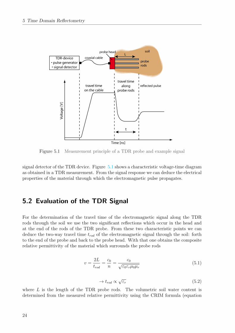
A schematic description of a TDR measurement system is shown in figure 5.1. It consistsof a TDR device which is composed of a signal generator and a sampling unit, and a TDRprobe that is connected to the TDR device via a coaxial cable. The system applied inthis practical course is controlled by a computer.

The measurement principle is based on the measurement of the propagation velocity of astep voltage pulse along a TDR probe through the ground. The probe is installed such,that the metal rods are completely surrounded by the soil material. In this experiment,we apply 3-rod TDR probes where the probe rods are arranged in a horizontal plane witha constant separation between the rods. In principle, the probe rods can be regarded asan elongation of the coaxial cable where the middle rod is the inner conductor and theouter rods represent the outer conductor of the cable. The TDR device generates shortelectromagnetic pulses (frequency range: 20 kHz to 1.5 GHz) which propagate along thecoaxial cable and further along the rods of the TDR probe. At positions where erraticchanges in relative permittivity occur, part of the electromagnetic energy is reflected.This is why TDR was initially developed for detecting failures along transmission linecables - TDR devices are also known as “cable testers”. The application in soil science is amodification of this technique. At the head of the TDR probe, part of the electromagneticenergy is reflected due to the impedance jump between the cable and probe head material.The remaining fraction of the signal propagates through the soil along the metal rodswhich serve as a wave guide. At positions where the dielectric properties of the soil changeerratically, the signal is again partially reflected. In soils with low electrical conductivity,the remaining part of the electromagnetic energy is finally reflected at the end of theprobe rods.

The temporal development of the voltage of the reflected TDR signal is recorded by the

23


Figure 5.1 Measurement principle of a TDR probe and example signal

signal detector of the TDR device. Figure 5.1 shows a characteristic voltage-time diagramas obtained in a TDR measurement. From the signal response we can deduce the electricalproperties of the material through which the electromagnetic pulse propagates.

5.2 Evaluation of the TDR Signal

For the determination of the travel time of the electromagnetic signal along the TDRrods through the soil we use the two significant reflections which occur in the head andat the end of the rods of the TDR probe. From these two characteristic points we candeduce the two-way travel time trod of the electromagnetic signal through the soil: forthto the end of the probe and back to the probe head. With that one obtains the compositerelative permittivity of the material which surrounds the probe rods

v =2L

trod=c0

n=

c0√ε0εrµ0µr

(5.1)

→ trod ∝√εr (5.2)

where L is the length of the TDR probe rods. The volumetric soil water content isdetermined from the measured relative permittivity using the CRIM formula (equation

24

5.3 Measurement Volume

Figure 5.2 Travel time determination from the TDR signal

4.3).

The reflection from the probe head is independent of the material between the probe rodsan hence occurs always at the same travel time and serves as a reference in the traveltime calculation. The travel time of the reflection from the rod ends depends on thepropagation velocity of the electromagnetic wave through the soil. The difference of thesetwo reflection points determines the travel time of the electromagnetic signal forth andback through the soil.

The travel time composes of the travel time through the probe head and along the proberods:

tprobe = thead + trods. (5.3)

For an accurate determination of the soil’s relative permittivity the TDR probes first haveto be calibrated in media with known propagation velocities. In our case the calibrationis done by conducting TDR measurements in water and air and correcting for the traveltime in the probe head.

Determination of the travel time of the electromagnetic signal is done by using the deriva-tive of the TDR signal and taking the largest values of the derivative occurring at theimpedance jump in the probe head and at the end of the rod as reference points (seefigure 5.2).

5.3 Measurement Volume

The measurement volume of a TDR probe is the volume of soil which has an influence onthe measured TDR signal.

25


Figure 5.3 Volume fractions of the total sampling volume (a) rod distance :rod diameter = 10 (b) rod distance : rod diameter = 5

The sensitivity of the TDR probe decreases exponentially perpendicular to the rod axes.The volume fractions shown in figure 5.3 are determined by the probe geometry and areindependent of the permittivity of the surrounding material. The measurement volumeis primarily determined by the diameter and the distance between the probe rods: anincrease in rod diameter leads to a smaller measurement volume; a larger rod distancecauses a stronger attenuation of the high-frequency components of the TDR signal andhence a smaller measurement volume.

5.4 Concluding Remarks

TDR probes can be installed vertically and horizontally in the soil. This way, one can in-vestigate the complete profile down to a depth of a few meters. As discussed in section 5.3the effective measurement volume of a TDR probe is relatively small. Hence, water con-tents determined from this method only represent local point measurements. For a spatialanalysis of soil water content at the field scale a huge number of measurements is required.Furthermore, one has to apply adequate interpolation techniques in order to obtain mean-ingful spatial information about water content distribution. Nevertheless, TDR is still astate-of-the-art technique in classical soil physics.

In order to obtain a good TDR measurement it is necessary to establish a good contactbetween the soil and the probe rods and to avoid air gaps during installation.

In this practical course we exclusively measure average soil moisture content along theprobe rods even if the water content may be changing. Currently inverse techniques arebeing developed in soil physics which allow to model the TDR signal and estimate spatialchanges in soil moisture content along the TDR probe. However, these techniques arecomputationally intensive and still in a development state and cannot be applied in theframework of this practical course.

26

6 Introduction to modeling

6.1 Introduction

Understanding nature requires detailed observation of interesting phenomena, develop-ment of possible hypotheses, and finally the testing of these hypotheses with experiments.The results of this investigation eventually converge to a representation of the phenomenonwhich allows the prediction of future system states. Thus, the major step towards a quan-titative understanding of a phenomenon, is the abstraction of the real world in such waythat our mind can grasp it and that we can develop intuition (see also figure 6.1).

6.1.1 Forward model

As physicists, we therefore exploit the mathematical language to build models. The firststep is the decision for a certain scale in space and in time1 in which the phenomenon hasto be represented. This decision is necessary, as we have to introduce (i) state variablesand (ii) material properties for the description of sub-scale properties and processes. Sub-sequently, we can use these state variables2 to formulate principle physical conservationlaws3. Afterwards, the most prominent processes4 are inserted into the conservation law,leading to a first mathematical model5.In order to use this mathematical model, we need information about the material proper-ties6. As these material properties represent sub-scale processes, they are mostly describedwith heuristic relationships7 which are inferred from measurement series. Note that ingeneral material properties vary in space and in time8 and it is very expensive (if notimpossible) to determine them directly!From an abstract point of view, the system which we investigate can be represented bythe following set: {mathematical description, state of the system, material properties9,

1e.g., time (ns, ms, s, h, y, . . . ) and in space (nm, mm, m, km, . . . )2e.g., water content θ3e.g., conservation of mass (continuity equation): ∂tθ +∇~j = 04e.g, an empirical flux law (Fick’s law): ~j = −K(θ)∇ψw(θ)5e.g., Richards equation6e.g., ψw(θ),K(θ)7e.g., ε′water(T ) but also ψw(θ) and K(θ)!8e.g., ψw(θ)→ ψw(θ, ~x, t) and K(θ)→ K(θ, ~x, t)9These include everything that is connected with the materials: The parameterization of effective ma-

terial properties, the parameters of the parameterization, and the distribution of the materials

27


Figure 6.1 A model helps to transform reality into a comprehensive structure withwhich reality can be understood by the mind. (The figure was adoptedfrom Kurt Roth via personal communication.)

boundary condition10}. Let us call this set representation of a system or model.

6.1.2 Inversion

In general, material properties are hard to measure directly but yet they are crucial for theapplication of a model. If we have no a priori knowledge about the material properties -which is the normal case - how can we get along? Note that the set given as the definitionof a model (see section 6.1.1) is overdetermined. This means, that if we knew for examplethe correct mathematical description, material properties and distribution, and boundarycondition, we could predict the state of the system and thus the measurements11.As the state of the system can be approximated with measurements, we may also changethe perspective and assume that the state is known but for example the material prop-erties are to be estimated. This is the standard parameter estimation procedure whichis also called inversion, regression or fit. Be aware, that this procedure also works forestimating every other component of the set, as long as all other components are known.To demonstrate this approach, the inversion method is illustrated shortly in the following.A typical approach to estimate the material properties is to realize an experiment and tomeasure at least one state variable12. Afterwards, a model is set up which implementsthe most important aspects of the experiment. After defining a measure for the distancebetween the simulated and the measured state variables (objective function), simulationsfor a variety of different material properties are executed and evaluated with the objec-tive function. Those material properties which minimize the objective function in theparameter space should be near the true material properties, if the assumptions made13

are true.

10In the sense of space and time, the boundary conditions also include the initial condition.11We can only measure the state in combination with one realization of the measurement error at a time.

Assume that the measurement error can be described as a statistical process with a certain probabilitydensity function. If we knew the shape of this probability density function and if we measured thestate N →∞ times, we could relate the expectation of the measurements and the state.

12e.g., water content θ13The most crucial assumption is that all other compartments of the model are perfectly known. De-

pending on the choice of objective function, additional assumptions have to be met.

28

6.1 Introduction

6.1.3 Data Assimilation

If you lean back and behold the problem of providing a consistent description of soil waterdynamics at a real test field, e.g., the ASSESS site14, you will find yourself asking severalquestions such as:

• How can we determine if the mathematical description is correct? How many phys-ical processes have to be included (think about the processes that compose theinteraction of soil, atmosphere, plants, animals, microbiological organisms, . . . )?.

• How can we determine if the representation of the material properties is correct?Which hydraulic parameterization model has to be applied? Can these simple pa-rameterization models even describe the whole three dimensional reality adequately?

• How can we determine measurement errors? How can we specify the precision andthe accuracy (distance to true state variable) of the measurements without knowingthe ground truth?

• How can we determine the subsurface material distribution? Do we even haveeffectively homogeneous material properties?

• How can we determine if the boundary conditions are correct?

• How can we determine the initial state of the system - not only at the position ofthe measurement sensors but also between them?

Thus, it should get obvious that the assumption that each but one component of themodel is completely known does not hold in general. In fact, each component is onlypartly known due to measurement errors, simplifications and assumptions deriving themathematical model and the material properties.Therefore, we have to use a combination of the information present in the model and inthe measurements to gain a consistent description of soil water movement. This is one ofthe fields on which we currently focus our research activities on.The combination of the information can be implemented naively as an iterative processfollowing Occam’s Razor 15:

1. Start with the simplest model and measurement procedure.

2. Compare model and measurements, learn, improve model and measurement proce-dure16.

3. While the model data and measurement procedure is not good enough, go to step2.

However, this approach is subjective since the actions compare, learn, improve depend on

14A detailed introduction of this measurement site is given in section A on page 59.15Roughly: Start with the simplest approach possible and improve it if you are forced to.16This includes the sampling rate, measurement position and type, . . .

29


the responsible person. Thus, such a learning procedure must be improved and objectified.This is achieved by the application of Data Assimilation methods which compare thesimulation with the measurement data at each measurement time and add a correctionsignal to the simulation depending on the measurement error, the model error, and thedifference between the measurement data and the simulation. This correction signal canhint at missing processes which then have to be implemented to improve the model.More information about data assimilation in hydrology is given by Liu and Gupta (2007).

6.2 Inversion of non-linear models

The main idea of inversion was already introduced in section 6.1: The representationof a real system (model) which is given by the set {mathematical description, state ofthe system, material properties17, boundary condition18} is overdetermined. Thus, theset is solved for the material properties19, exploiting the measurements to approximatethe system state. Therefore, all inversion methods rely on the assumption of perfectknowledge of all the other components of the model20.

As qualitatively outlined in section 6.1.2, a measure for the distance between the simula-tion and the measurements has to be defined.One popular choice of the objective function is the following:

χ2(~p) =i=N−1∑i=0

[yi − y(~xi, ~p)]2

σ2i

, (6.1)

where yi represents one of the in total N measured data points, each associated withits position ~xi and standard deviation σi. These measured values are subtracted by thesimulated values y(~x, ~p) for a given parameter set ~p.Note that the assumption of white gaussian measurement noise with standard deviationσi is implicitly made by choosing this definition of objective function. The result of theobjective function χ2 is called residual or residuum.

Two popular methods for the inversion of non-linear models21 will be outlined subse-quently.

17These include everything that is connected with the materials: The parameterization of effective ma-terial properties, the parameters of the parameterization, and the distribution of the materials

18As this is in the sense of space and time, the boundary conditions also include the initial condition19or any other component of the representation of the real system20In general this assumption is not valid. Missing processes, heuristic material properties, not directly

measurable boundary conditions, simplifications, assumptions and approximations lead to systematicerrors. Additionally, measurement errors are biased in general or may even drift, e.g., with time andtemperature

21As the Richards equation is highly non-linear, these comparably computationally expensive methodshave to be applied. For linear cases, the inversion method comes down to solving the linear equationsystem A~x = ~b for ~x. This can be solved by (iteratively, approximately) inverting the matrix A, forexample with the Gauss-Jordan algorithm.

30


p

𝟀2

pi

Steepest Descent

Gauss-Newton

X

pi+1 pi+1 pipi+∆p

XX

X

X

pi+∆p

X

Figure 6.2 The Levenberg-Marquardt algorithm is applied for iteratively searchingthe minimum of the objective function (e.g., χ2(p)) in the parameterspace. The algorithm is very robust, because it moves continuously be-tween the Gauss-Newton and the Steepest Descent algorithm dependingon the success of the current iteration. Both algorithms approximatethe local gradient ∇χ2 by the local difference quotient with the displace-ment ∆p. In general, the form of the objective function χ2(p) is notknown a priori. The Gauss-Newton assumes a parabolic shape and ex-ploits the local gradient to estimate the parameter set for the minimumof the parabolic shape. The Steepest Descent algorithm just follows thenegative gradient. In this figure, one iteration of these two algorithms issketched, starting from parameter pi.

Levenberg-Marquardt

This method is one of the standard optimization algorithms for solving non-linear prob-lems, because it is relatively efficient. Its main strength is, that it enables a continuoustransition between the Gauss-Newton and the Steepest Descent algorithm.The assumption behind the Gauss-Newton algorithm is that the shape of the residuumhas parabolic shape near the global minimum. Thus, the position of the parameter set atthe minimum can be calculated directly.If this assumption does not hold, the most trivial way of reaching the minimal residuumin the parameter space, it to calculate the gradient of the residuum and to follow thenegative gradient. A sketch of this idea is presented in figure 6.2.

In the remaining part of this section, the Levenberg-Marquardt algorithm is explored ina more formal way which follows the line presented by Press (2007).Deriving the Gauss-Newton algorithm, it is assumed that the χ2(~p) function can be ap-

31


proximated by a quadratic form

χ2(~p) ≈ γ − ~d · ~p+1

2~p ·D · ~p, (6.2)

where the parameter vector ~p has M entries, the matrix D is a M ×M matrix, and γ isa scalar.Starting with the current parameter set ~pcurrent, the parameter set ~pminimal where χ2(~p) isminimal can be calculated directly via

~pminimal = ~pcurrent −D−1 ·[∇χ2(~pcurrent)

].22 (6.3)

The current parameter set ~pcurrent can also be improved by following the negative gradientof χ2(~pcurrent), which leads to

~pnext = ~pcurrent − c · ∇χ2(~pcurrent) (6.4)

with a scalar constant c.

The partial derivative of the objective function (equation 6.1), which has to be zero atthe minimum of χ2, has the components

∂χ2

∂pk= −2

N−1∑i=0

[yi − y(~xi|~p)]σ2i

∂y(~xi|~p)∂pk

(6.5)

for k = 0, 1, . . . ,M − 1. The calculation of the Hessian matrix D, requires to take anadditional derivative which yields

∂2χ2

∂pk∂pl= 2

N−1∑i=0

1

σ2i

[∂y(~xi|~p)∂pk

∂y(~xi|~p)∂pl

− [yi − y(~xi|~p)]∂2y(~xi|~p)∂pl∂pk

]. (6.6)

It is conventional to remove factors of 2 in the equations 6.5 and 6.6 by defining

αk ≡ −1

2

∂2χ2

∂pk∂pland

βk ≡ −1

2

∂χ2

∂pk.

(6.7)

22See also the Newton-Method:

• Taylor expansion of function f(x) around xi: f(x) ≈ f(xi)+(x−xi)·∇f(xi)+ 12 (x−xi)·A·(x−xi),

where the matrix A is an approximation of the Hesse matrix

• ∇f(x) = ∇f(xi) +A(x− xi)

• At the extremum, the gradient has to vanish: ∇f(x) = 0, leading to

• x = xi −A−1 · ∇f(xi)

32


With α = 12D, the parameter update equation for the Gauss-Newton algorithm (equa-

tion 6.3) can be rewritten as the linear equation

M−1∑l=0

αklδpl = βk (6.8)

for the increments for the parameters δpl = pl,next − pl,current.Inserting α and β in the parameter update equation for the Steepest-Descent algorithm,equation 6.4 becomes

δpl = c · βl. (6.9)

The calculation of the Hessian matrix (equation 6.6) can be simplified, since the depen-dency of αkl on the second derivative is supposed to be small compared to first derivative.This is because the second derivative is multiplied by the factor [yi − y(~xi|~p)] and for asuccessful model, this factor has the size of the random measurement error. Therefore, itshould cancel out when summed over i. Thus, the second derivative is neglected whichleads to

αkl =N−1∑l=0

1

σ2i

[y(~xi|~p)∂pk

∂y(~xi|~p)∂pl

]. (6.10)

Note that the condition βk = 0 for all k is independent of the definition of α.

The Levenberg-Marquardt algorithm bases on two important insights.The first one concerns the constant c in equation 6.4. Apriori, it is unclear how tochoose the scale and its magnitude. However, the Hessian matrix contains at least someinformation about how to choose this constant. As χ2 is non dimensional and βk hasdimension 1/pk

23, the dimension of c has to have the dimension a2k. The only one quantity

in matrix alpha that matches this dimension is 1/αkk which is the reciprocal of the diagonalelement. Yet, the scale of this value might be too big. Therefore, it is divided by a fudgefactor λ. Hence, equation 6.9 is replaced by

δpl =1

λαllβl or

λαll δpl = βl,(6.11)

where αll have to be positive. Note that this is guaranteed by the approximation madein equation 6.10.The second insight is that the equations 6.8 and 6.11 can be combined by defining a newmatrix α′ (sensitivity matrix)

α′jj ≡ αjj(1 + λ)

α′jk ≡ αjk,(6.12)

23Note, that each component has a different dimension in general.

33


which replaces both equations 6.8 and 6.11 by

M−1∑l=0

α′klδpl = βk. (6.13)

For large λ, the matrix α′ is forced to be diagonally dominant, so equation 6.13 goes overto be identical with equation 6.11. On the other hand, if λ is zero, equation 6.13 becomesequation 6.8.

With an initial guess for the parameter set ~p, the Levenberg-Marquardt algorithm worksas follows:

1. Compute χ2(~p)

2. Pick a modest value for λ, for example λ = 0.001

3. Solve the linear equations 6.13 for δ~p and evaluate χ2(~p+ δ~p)

4. If χ2(~p+ δ~p) ≥ χ2(~p), increase λ by a factor and go back to point 3

5. If χ2(~p + δ~p) < χ2(~p), decrease λ by factor, update the trial solution ~p ← ~p + δ~p,and go back to point 3

There are different ways to break this loop, e.g., if either

• a lower limit for χ2(~p),

• a lower limit for the improvement of χ2(~p) during one iteration,

• a lower limit for the parameter correction δ~p24,

• an upper limit for λ, or

• an upper limit for the number of iteration

is reached. Most often, a combination of these conditions is implemented.

As soon as the algorithm is converged, λ is set to zero and the covariance matrix of theparameters is calculated from the approximation of the Hesse matrix via

C ≡ α−1. (6.14)

If the measurement errors are normally distributed, the square root of the diagonal entriesof this covariance matrix C can be understood as the standard error of the parameters.If the assumption does not hold, then there is another possibility to estimate confidencelimits of the estimated parameter set ~pbest: Take the parameter set ~pbest and solve theforward problem. Then, create a number of synthetic measurement data sets by addinga different realization of measurement noise to this solution. Use these synthetic mea-

24In practice, one would rather define a lower limit for the relative parameter correction.

34


surement data sets to estimate new parameter sets, which will give you an idea of theconfidence limits of the resulting parameter set.

Be aware, that there is the problem of the local convergence of the algorithm. As thealgorithm exploits the gradient of χ2, the initial parameter set has to be close to the trueparameter set to ensure convergence to the global minimum. If the start parameter forthe Steepest Descent algorithm in figure 6.2 had been slightly larger, than the algorithmwould have converged to the local minimum on the right hand side. One way to investigatethe corresponding convergence radius to the problem at hand is to generate a number ofrandom initial parameter sets25 and to start the inversion from these. The resultingparameter sets will give an idea, how the minima are distributed in the parameter spaceand how large the convergence radius may be. This method is quite costly, however.

More information about the Levenberg-Marquardt algorithm - besides other fine informa-tion about mathematical methods and their implementation - is given by Press (2007)26.

Shuffled Complex Evolution

The Shuffled Complex Evolution algorithm proposed by Duan et al. (1994) is a standardparameter estimation algorithm that overcomes one problem of the Levenberg-Marquardtalgorithm because it is globally convergent. However, it is relatively slow compared tothe Levenberg-Marquardt algorithm but comparably fast compared to other globally con-vergent methods. It is remarkable, that the formulation of this algorithm is inspiredby evolution as it exploits the iterative separation of the population into independentsub-populations where the individual members are improved separately only to finallycompete agains the members of the other sub-populations.

The algorithm may be sketched as follows:

1. Generate an ensemble of models27.

2. Divide the ensemble in a number of complexes (subsets of the ensemble).

3. Improve members of the complexes separately:Propose a new member by reflecting the worst member of the complex the throughthe centroid of the other members of the complex (reflection step)28. If the proposedmember is not better than the worst, make the contraction step29 which proposesa member which lies halfway between the worst member and the centroid of theother members. If this step is unsuccessful as well, try the mutation step where theparameters are sample randomly until a member is found which is better than the

25e.g. uniform distribution or better sampling with Orthogonal Latin Hypercubes26The relevant chapter is called Modeling of Data and starts at page 773.27Give each ensemble member a different parameter set28The parameter α > 0 determines the width the reflection step.29The parameter β > 0 determines the width the contraction step.

35


worst member.

4. Break up the complexes and sort all ensemble member according to the associatedresiduum.

5. Shuffle the members in complexes30 again and go to point 3.

More information about the Shuffled Complex Evolution algorithm is given by Duan et al.(1994).

Residuum scanner

This algorithm was implemented to explore objective function by iterating over one pa-rameter within its specified range while keeping the other parameters constant. Theobjective function is then evaluated for every iteration.

Although it is really expensive, the tool is useful to explore the over all behavior ofthe objective function. However, keep in mind that χ2(~p) is explored only in one ortwo dimensions which means that by changing the other parameters, the shape of χ2(~p)changes in general.

Regardless of these facts, it is a nice example to illustrate the Curse of Dimensional-ity31. For example assume, that our problem at hand has d dimensions and we choose edevaluations per dimension which makes the total number of evaluations et = edim

d. Thismeans, for d = 6, edim = 10 and te = 30 s for the solution of one forward problem, thescan would take 8333 h or 374 d32. If we like to compare that to the performance of theLevenberg-Marquardt algorithm (let us assume it took i = 40 iterations to converge), itwould have take i · (d+ 1) · te = 2.3 h to find the minimum - but only if the requirementsfor the Levenberg-Marquardt algorithm are met33. In figure 6.3, the results of for a highlyresolved (edim = 100) run of the residuum scanner is presented.

30If the ensemble has 12 members and is divided in 3 complexes, member 1 goes into complex 1, member2 goes into complex 2, member 3 goes into complex 3, member 4 goes into complex 1, member 5 goesinto complex 2 and so forth.

31See also https://en.wikipedia.org/wiki/Curse_of_dimensionality32Typical values for research problems in our group are d ≥ 18 and te ≥ 300 s leading to a total run time

tt ≥ 9.6 · 1020 a to complete. In comparison, the age of the universe is approximately 13.8 · 109 a.33These include that the initial parameter set is located in a convex region of the objective function

which also includes the global minimum of the objective function

36

https://en.wikipedia.org/wiki/Curse_of_dimensionality


Lam

bda

Air Entry Value

Residuum (log10)

0.5

1

1.5

2

2.5

-0.12 -0.1 -0.08 -0.06 -0.04 -0.02 3

3.5

4

4.5

5

5.5

6

Lam

bda

Air Entry Value

Residuum (log10)

0.5

1

1.5

2

2.5

-0.12 -0.1 -0.08 -0.06 -0.04 -0.02 3

3.5

4

4.5

5

5.5

6

Figure 6.3 Scan of the residuum over two parameters of the Brooks-Corey parame-terization. Top: Residuum for each resulting point of the scan, Bottom:Bilinear interpolation between the resulting points.

37


38

7 Exercises

In this part of the practical course, you will get hands-on modeling experience with thesoftware which we develop to address our research questions.The software SHIP (Soil-Hydraulics and Hydrogeophysics Inversion Package) expands andwraps two forward models:Muphi (µϕ)1 solves the Richards equation using a cell centered finite volume scheme withfull upwinding in space and an implicit Euler scheme in time. The linearization of thenonlinear equations is done by an inexact Newton-Method with line search. The linearequations are solved with an algebraic multigrid solver.Maxwells equations are solved for the simulation of GPR radargrams with the freelyavailable software package MIT Electromagnetic Equation Propagation (MEEP) whichwas introduced by Oskooi et al. (2010). This software exploits the Finite-Difference Time-Domain (FDTD) method proposed by Taflove and Hagnes (2005).Both codes are physics-based, can operate in 1, 2, or 3 dimensions, and are able to runefficiently on the largest available computers.

7.1 General Remarks

Initially, some general remarks are in order.

• Before you start modeling, always ask yourself the following questions: What isthe question that has to be addressed? What is the expected outcome? Write theanswers to these questions in your notebook to ensure the required focus and theassociated learning process. Be sure to always think about what you expect to bethe results of your simulation. To straighten these thoughts, write them down. Ifthe results of the simulation do not correspond to your expectation, investigate whythis is the case.

• The program is controlled with an input file (control.ini) which contains keys andassociated values. To execute the program, open the Terminal2, navigate to thefolder3, specify the keys in the control file, and then execute the program4.

1This code was written by Dr. Olaf Ippisch, IWR Heidelberg2You will find it in Programme → Dienstprogramme3Just type cd and then drag the folder from the Finder to the Terminal window to get the path to this

folder.4To simplify the execution of the program, bash-scripts (suffix .sh) are prepared to help you with that.

Please open them, understand them and then execute them via ./ <name of the script>

39

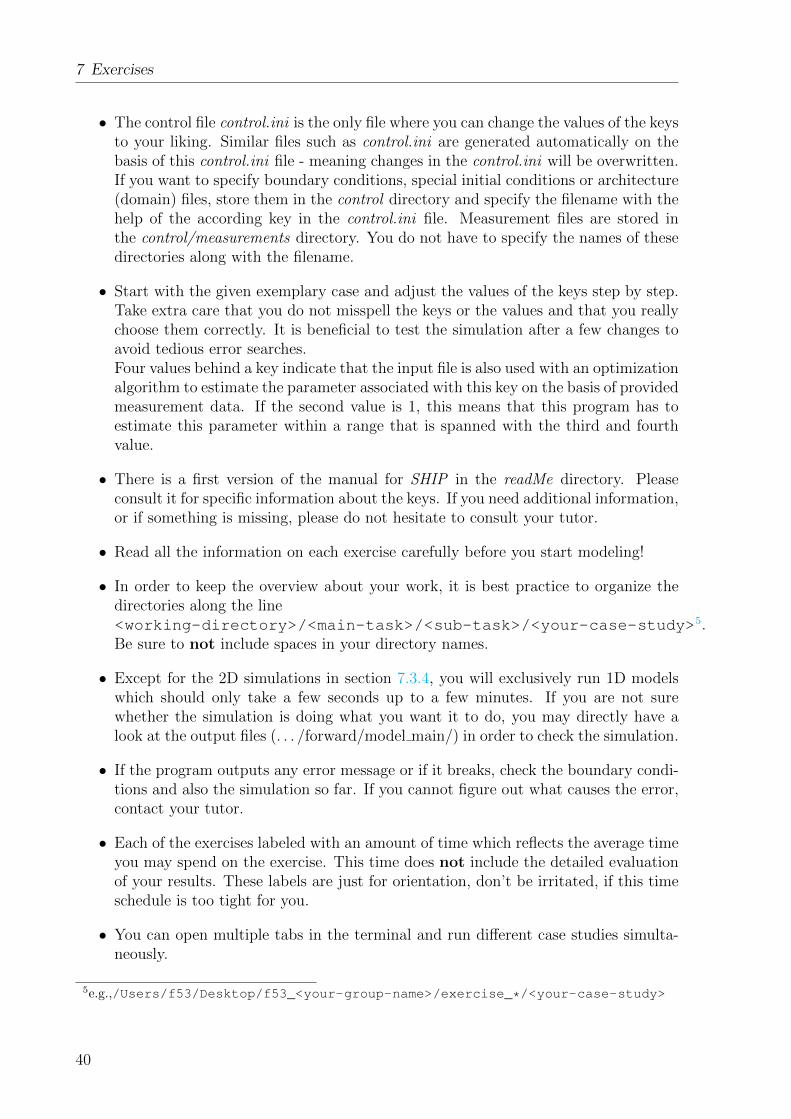
7 Exercises

• The control file control.ini is the only file where you can change the values of the keysto your liking. Similar files such as control.ini are generated automatically on thebasis of this control.ini file - meaning changes in the control.ini will be overwritten.If you want to specify boundary conditions, special initial conditions or architecture(domain) files, store them in the control directory and specify the filename with thehelp of the according key in the control.ini file. Measurement files are stored inthe control/measurements directory. You do not have to specify the names of thesedirectories along with the filename.

• Start with the given exemplary case and adjust the values of the keys step by step.Take extra care that you do not misspell the keys or the values and that you reallychoose them correctly. It is beneficial to test the simulation after a few changes toavoid tedious error searches.Four values behind a key indicate that the input file is also used with an optimizationalgorithm to estimate the parameter associated with this key on the basis of providedmeasurement data. If the second value is 1, this means that this program has toestimate this parameter within a range that is spanned with the third and fourthvalue.

• There is a first version of the manual for SHIP in the readMe directory. Pleaseconsult it for specific information about the keys. If you need additional information,or if something is missing, please do not hesitate to consult your tutor.

• Read all the information on each exercise carefully before you start modeling!

• In order to keep the overview about your work, it is best practice to organize thedirectories along the line<working-directory>/<main-task>/<sub-task>/<your-case-study>5.Be sure to not include spaces in your directory names.

• Except for the 2D simulations in section 7.3.4, you will exclusively run 1D modelswhich should only take a few seconds up to a few minutes. If you are not surewhether the simulation is doing what you want it to do, you may directly have alook at the output files (. . . /forward/model main/) in order to check the simulation.

• If the program outputs any error message or if it breaks, check the boundary condi-tions and also the simulation so far. If you cannot figure out what causes the error,contact your tutor.

• Each of the exercises labeled with an amount of time which reflects the average timeyou may spend on the exercise. This time does not include the detailed evaluationof your results. These labels are just for orientation, don’t be irritated, if this timeschedule is too tight for you.

• You can open multiple tabs in the terminal and run different case studies simulta-neously.

5e.g.,/Users/f53/Desktop/f53_<your-group-name>/exercise_*/<your-case-study>

40

7.2 Tools

Figure 7.1 Application of the Plot Over Line filter in ParaView

7.2 Tools

7.2.1 ParaView

In this course, the visualization of the simulated data is mainly done with ParaView 6.

Apply button

In order to visualize the resulting *.vtr files of the simulation, openParaView ( ), click on the top left icon ( ) to open the files youwant to visualize. ParaView directly groups files with the same prefix,so that you can open and visualize multiple files at once. If you justdouble-click on one file, then you will be able to visualize this single file.As soon as you opened the files, click Apply in the Properties window.Depending on the defined output variables in the simulation, you canchoose the data type to visualize via a drop-down menu ( ).To play the temporal evolution of the simulation, just use the play buttons ( ). It maybe convenient to automatically adjust the color scale in the current frame ( ). Be awarethat this color scale is then used also in the other frames if you play the simulation.You can also choose to plot the data along one line. Therefore, click on the files you opened(results * ), go in the top menu bar on the screen to Filter → Data Analysis → Plot overline. In the Properties window, you can specify the properties of the line (mostly youjust want to plot along the Y Axis - click on ). Then click on Apply, and afterwards

6available for all common operation systems for free viahttp://www.paraview.org/download/

41

http://www.paraview.org/download/

7 Exercises

you can specify the variables to plot. Therefore, click on the window in ParaView whichshows the line plot in order to activate it in the Properties window. Then scroll down inthe Properties window and select the variable of interest in the drop-down menu X ArrayName and select arch length in the Series Parameters field. You can adjust the range ofthe axis in the fields Left Axis Range and Bottom Axis Range.If you want to export the active visualization to pdf, go in the top menu bar on the screento File and then to Export Scene (choose pdf as file type).

42

7.3 Hydraulic Modeling


7.3.1 Mualem-Brooks-Corey material functions (≈ 1 h)

Goals The main focus of this practical course is on soil hydraulic material properties.Therefore, you will get acquainted with one of several parameterization models in thisintroductory exercise. The Mualem-Brooks-Corey parameterization model is widely ap-plied to describe the hydraulic material properties of unsaturated soils as the associatedparameters may be related to microscopic properties of the soil structure (see also figure7.2).The main task of this exercise is to understand the mathematical formulation of theMualem-Brooks-Corey parameterization model, its connection to the Richards equationand the physical implications of its parameters.

Additional Information In order to simplify this exercise, a gnuplot script was preparedfor you, which plots the hydraulic material functions based one reference parameter set.Additionally, each parameter is changed for a specified number of times while all otherparameters fixed to the reference parameter set leading to a set of similar functions.With the help of this script, you can get a feeling how the material parameters changethe material functions.

Tasks

1. Revisit chapter 2.3 and understand the equations 2.15 and 2.23.

2. Open the Terminal and change to the directory of this exercise (exercise 01 )

3. Open the file ’plotMualemBrooksCorey.gpt’ and try to understand how it is used.

4. Run the run.sh script which executes gnuplot to produce plots of the hydraulicmaterial functions that are then directly stored as *.pdf files in the directory of theexercise.

5. Investigate these resulting plots and describe how each parameter is changing thehydraulic material functions.

6. Try to relate these curves to the real physical system. Which physical propertiesare responsible for the different characteristics of these material functions?

Questions

1. Which information do you need to specify if you like to solve the Richards equationfor a given system?

43

7 Exercises

��

��

��

��

��

��

��

��

��

��

��

��

��

��

��

��

��

��

��

��

��

��

Figure 7.2 Exemplary Mualem-Brooks-Corey material functions for the parametersets that may be associated with sand and silt (see also table 7.1).

2. How do the hydraulic material functions enter the Richards equation?

3. Which state variables are described with these material functions and what is thephysical meaning of these state variables?

4. What micro- and macroscopic physical properties of the soil do influence the formof these material functions? Can you relate each parameter with a macroscopicphysical property of the soil?

7.3.2 Soil water dynamics in homogeneous materials (≈ 2h)

Goals The main task of this exercise is to explore and to explain the non-linear reactionof the hydraulic system to the different boundary conditions, namely the fluctuating watertable and the infiltration front for two different characteristic homogeneous materials (sandand silt).

Additional Information We will basically focus on two different ways to force the systemof interest its the boundaries:

Table 7.1 Exemplary Mualem-Brooks-Corey parameter sets to describe soil hy-draulic properties of sand and silt (Carsel and Parrish, 1988).

θs θr h0 [m] λ K0 [m s−1] τsand 0.43 0.045 -0.069 1.68 8.25 · 10−5 0.5silt 0.46 0.034 -0.625 0.37 6.94 · 10−7 0.5

44


• Neumann:This boundary condition prescribes a boundary flux which may be used to modelinfiltration, evaporation, and also a fluctuating water table. Whenever you aredealing with this boundary condition type, you have to make sure that the systemis able to maintain the prescribed flux at the boundary.

• Dirichlet:This boundary condition prescribes a potential (matric head) at the boundary. Youmay imagine a huge water reservoir leading to a given potential at the specifiedboundary. In this practical course, this boundary condition type is mainly used tomodel the groundwater table at a certain depth. However, this boundary conditionmay also be applied with a negative potential to model, e.g., evaporation.

The boundary condition has to be specified in a separate file which is located in the controldirectory. You are free to choose a filename of your liking but this filename has to bespecified in the control.ini file via the key hydr boundary condition file. The boundarycondition file has the following structure:

bound cond north 1 0

bound cond south 1 1

bound cond west 0

bound cond east 0

num times 2

0 neumann -1e-7 neumann 0


The boundaries of the two dimensional domain are named in the following way: Northrepresents the upper, south the lower, east the right, and west the left boundary. Thenumber behind the orientation specifiers (e.g., bound cond north) give the number ofsections with a distinct boundary condition on the according boundary edge. In thisexercise here, the boundary condition is the same on the whole extent of the boundaryedge, hence the number is set to 1. This number is followed by a global index of bound-ary conditions which is used to associate each section on the boundary edge with theprescribed boundary condition for each time. Beware that this global index starts with0: In the given example, the boundary condition on the northern edge has index 0 andthe boundary condition at the southern edge has index 1. If we do not want to define anyspecific boundary condition, the number of boundary conditions on this boundary is setto 0. This leads automatically to a neumann boundary with flux 0.0 m/s.The key num times defines the number of lines in the file where the boundary conditionsat all the sections are associated with a specific time. These lines always start with thetime which is then followed by a boundary condition type and its associated value foreach global boundary section index. It is necessary that for each index specified in theheader of the file, one boundary condition (type and value) is given for each time. Note,that the given times mark subsequent absolute points in time.If two different times with the same boundary condition type but an different boundarycondition value follow upon each other, the boundary condition is interpolated betweenthese times. If you want to switch the boundary condition type at a given time, then youhave to specify the boundary condition for this time twice (see time 7200):

45

7 Exercises



7200 dirichlet 0.1 neumann 0



Also keep in mind, that the boundary flux of the neumann boundary condition has to bespecified relative to the normal direction of the boundary. This means that a negativevalue for the boundary flux leads to a flux into the system. The unit of the neumann fluxis [m/s] and the unit of the dirichlet potential is [m].

The size of the domain on which we solve Richards equation in this exercise is suggestedhave a vertical extent of 4 m, corresponding to 800 grid cells - leading to a resolution ofone grid cell per 0.5 cm. This is done by setting the key domain gridpoints to 1 800 andthe key domain size to 1.0 4.0, respectively. The first value refers to the x (horizontal)and the second value to the y (vertical) dimension.

For all the simulations of this exercise, be sure to output the water content as well as thematric head by setting the key hydr output variables at least to thetal pl.

To run the simulation, always copy the directory from the examples to a working directoryof yours. This ensures that you always have access to the provided working example. Inorder to keep the overview about your work, it is best practice to organize the directoriesalong the line<working-directory>/<main-task>/<sub-task>/<your-case-study>7.Each case study then consists of the control directory (containing the subsurface archite-cure, boundary conditions, initial conditions, possible measurement data, . . . ) and thecontrol.ini file as well as the run.sh script.

Tasks

1. Explore the soil water dynamics of a fluctuating water table

a) Copy the case study for this exercise to a working directory of your own.

b) Check whether the initial condition is specified as intended.

c) Check whether the subsurface domain is specified as intended.

d) Check whether the output variables are specified as intended.

e) In order to model a sandy material, set the keys in the corresponding keys inthe control.ini file to the parameters given in table 7.1.

f) In the control directory, setup a boundary condition file, where the ground

7e.g.,/Users/f53/Desktop/f53_<your-group-name>/exercise_02/fluctuatingWaterTable/<your-case-study>

46


water table is located at the southern boundary at time 0 and then rises linearlyto 2.1 m above the southern boundary in the course of 4 h (imbibition step).For further 20 hours, the ground water table should stay at 2.1 m (equilibrationstep), before it is decreased linearly to the southern boundary again over thecourse of another 12 h (drainage step). The boundary condition at the northernboundary is set to a neumann boundary condition with flux 0.0 m over thewhole period of time.

g) Based on your knowledge about the material properties, try to predict thewater content distribution and the potential water content distribution overthe height for each of the three steps (imbibition, equilibrium, drainage). Besure to note (where appropriate also sketch) your predictions in your notebook.

h) Subsequently, run the simulation and visualize the results with ParaView. Ashort introduction to this program is given in section 7.2.1. As ParaView willbe the tool for visualization in the next few exercises, be sure to read thissection carefully. For a better visualization of the hydraulic effects, choose thePlot over line filter.

i) Discuss the differences between your prediction and the simulation.

j) If you plot the water content distribution against the height, you should seetwo kinks during the imbibition step. Explain the mechanisms that lead tothese kinks.

k) Predict the behavior of the system for a silty material, record your predic-tions, and repeat the simulation with the silty material afterwards. Discussthe differences between your prediction and the simulation.

2. Explore the soil water dynamics of an infiltration front

a) Copy the case study for this exercise to a working directory of your own.

b) Check whether the initial condition is specified as intended.

c) Check whether the subsurface domain is specified as intended.

d) Check whether the output variables are specified as intended.

e) In the control directory, check for the bc.dat file, understand and describe theapplied boundary condition. Use this file for the simulation.

f) Be sure to set the simulation time hydr max time accordingly.

g) Try to predict the water content and the potential distribution for each of thethree characteristic steps (infiltration, equilibrium, evaporation). The bound-ary condition at the southern boundary is set to a dirichlet boundary conditionwith potential 0.0 m over the whole period of time.

47

7 Exercises

h) Subsequently, run the simulation and visualize the results with ParaView.

i) Discuss the differences between your prediction and the simulation.

j) Predict the behavior of the system for a silty material, record your predic-tions, and repeat the simulation with the silty material afterwards. Discussthe differences between your prediction and the simulation.

Questions

1. In what characteristic way does the water content distribution during the imbibitionstep differ from the one during the drainage step?

2. Explain why the infiltration front may be considered as self-sharpening.

3. Discuss the differences between the simulations for the sandy and the silty material.

4. With the gained insights into soil physics, discuss whether the sandy Sahara desertfavors groundwater recharge or not.

7.3.3 Soil water dynamics in layered media (≈ 1 h)

Goals The main task of this exercise is to explore and to explain the non-linear reactionof the hydraulic system to the boundary conditions applied in exercise 7.3.2, for a two-layer material distribution of sand and silt.

Additional Information As in the previous exercises, the simulation should start fromthe equilibrium initial condition with a ground water table at the southern boundary.

In oder to generate a architecture file which supports two materials, set the key do-main number materials to 2 and tell the software to generate an architecture file by settingthe key domain generate architecture asciifile to true. Naturally, we also have to spec-ify the name of the architecture file via setting domain architecture asciifile to architec-ture.dat. The software generates a layered medium if we set the keys domain generation modeto layers and domain generate 1d layers to true. Finally, the position of the material in-terface has to be specified by setting domain 1d layer height 1 to 2.0.

Be aware, that two distinct sets of material properties have to be specified. You canchange the association of the material number and the material properties simply withthe key hydr material greylevel 1 8.

For all the simulations of this exercise, be sure to output the water content as well as

8To associate material 1 with the parameter set with the index 1, just set hydr material greylevel 1 to1

48


the matric head by setting the key hydr output variables to thetal pl. Additionally, it isbeneficial for the visualization to set the hydr output interval to 3600 s.

Tasks

1. Create a case study with two layered materials. The position of the layer interfaceshould be half the height of the domain.

2. At first, associate the top material with sandy material properties and the bottommaterial with material parameters corresponding to silt. Use the hydraulic materialparameters given in table 7.1.

3. Create two different case studies with this subsurface material distribution: Onewith the fluctuating water table boundary condition from exercise 7.3.2 and onewith the infiltration boundary condition.

4. Remember to adjust the neumann boundary flux in the infiltration boundary condi-tion to 1/10 of the saturated hydraulic conductivity of the material where the fluxis applied.

5. Run the simulation and try to understand the temporal evolution of the watercontent and the matric head.

6. Now switch the position of the materials such that the silty material is located abovethe sandy material, repeat the exercise and compare the results with the previousmaterial distribution.

Questions

1. Why does the water content jump at the material interface even in stationary equi-librium?

2. Explain the temporal evolution of the water content and matric head in the materialsover time with your knowledge about the material functions (also figure 7.2).

3. Compare the results for the two material distributions.

7.3.4 Soil water dynamics in heterogeneous media (≈ 2 h)

Goals In this final exercise solely covering soil water dynamics, we investigate the soilhydraulic properties of a real but artificial structure: The ASSESS test site. As shown infigure 7.3, the structure of and consists of three distinct kinds of sands which model aneffectively 2D geometry. The soil bulk permittivity is measured with 32 Time Domain Re-flectometry (TDR) and soil temperature sensors. The ground water table is automatically

49

7 Exercises

Introduction Data Acquisition Measurement Data Model Assimilation Roadmap

Heidelberg UniversityInstitute of Environmental Physics

Stefan Jaumann [email protected]

A framework for constructive inversion of soil water dynamics on the basis of hydrogeophysical measurements

2014-07-08

3.3 Experiments 23

0

0.2

0.4

0.6

0.8

1

1.2

1.4

1.6

1.8

0 2 4 6 8 10 12 14 16 18

Hei

ght

[m]

Length [m]

8

7

6

5

4

3

2

1

25

26

27

28

29

30

31

32

18

19

20

21

22

23

24

9

10

11

12

13

14

15

16

17

A

B

C

C

B

A

Figure 3.4. Domain geometry for the numerical model presenting the distribution ofthe three materials A, B and C. Solid lines indicate material interfaces, whereas dashedlines indicate measured compaction interfaces. Circles represent the TDR sensors withtheir numbering. The sensors are partitioned in four profiles corresponding to theirhorizontal position. Sensors 1-8 represent profile 1, sensors 9-17 profile 2, sensors 18-24profile 3 and sensors 25-32 profile 4. The well is located at approximately 18.3 m.

into the well and extracting it afterwards. During this forcing at the lower boundarycontinuous GPR measurements were conducted on the surface.The boundary condition during these experiments is presented in the tables 3.1, 3.2 and3.3.

The experiment in September was designed for a stationary observation of the capillaryfringe with GPR measurements. Therefore, the antennas were situated at the two-layered

Table 3.1. Forcing of the imbibition and drainage experiment of September 2011 with48.0 cm initial water table

Start End Volume [m3] Minutes Flux [m3 min�1]

Imbibition 11:11:00 13:11:00 3.8357 120 0.0320Drainage 15:13:00 16:44:00 3.8002 91 0.0418

6 Results and Discussion

0240 5 10 15 20

−2

−1

0

x [m]y [m]

z [m

]

Figure 6.1: Three dimensional illustration of the geometry at the ASSESS-GPR testbed. Thelowest interface corresponds to the upper surface of the gravel layer while the sand surface isat the top. The green arrow represents the GPR measurement line (y-direction at x = 2.1m)and the red markers indicate the position of TDR probes. The probe centers are located atx = 0.8m, i.e., 1.3m besides the GPR line. A rotating view of the geometry is provided in themovie ASSESS_Geometry_3D.mp4.

were built into the volume and finally compacted using a vibrating plate (figure A.1b)to prevent compaction by the materials own weight after the building. The positionsof the layer interfaces were obtained with a TCRA1102 tachymeter (Leica GeoSystems,Germany) and by manual measurements (figure A.1c); hence ground-truth informationon the layer geometry is provided with a precision of 1 cm. However, the accuracy of theinformation when comparing with GPR-data is most-likely not better than 5 cm. Thereasons are (i) additional compaction of the sand layers during the building procedure,(ii) changes of the soil surface height by external influences, (iii) sinking of the GPRantennas into the sand, and (iv) the variations of geometry along the x-direction. Thelatter is relevant since the comparison is made between the 2D crosscut (figure 6.2) iny-direction and the evaluation of GPR data. The data, however, also include informa-tion transverse to the measurement line because of the three-dimensional propagationof the electromagnetic pulses in the subsurface.

Spatial or temporal changes in water content cause significant changes in the e�ectivedielectric permittivity of the sand-water-air mixture. In the unsaturated state, the watercontent across layer interfaces is discontinuous (figure 2.5) in most cases if the layers’hydraulic properties are di�erent due to variations of the pore-size distribution. On theone hand this can be induced by di�erences in the grain-size distribution, as given forthe materials build into the testbed (table A.1). On the other hand, spatial variationsof porosity, as possibly introduced by the compaction of the layers, a�ect the poregeometry. For both reasons jumps in dielectric permittivity are expected across theinterfaces in the testbed.

Dielectric permittivity of as well as direct current conductivity is observed at 32positions. This is done by temperature and TDR probes (figure 6.2). The latter have3 rods of 0.2 m length. The measurements are conducted on a regular basis by aTDR100 time-domain reflectometer (Campbell Scientific, UT, USA) which is part ofan automatic weather station.

The TDR probes were calibrated in the laboratory for dielectric permittivity andconductivity measurements. The evaluation for both quantities is conducted with stan-dard techniques [Roth et al., 1990, Heimovaara et al., 1995] employing signal traveltimeand attenuation, respectively.

78

2. ASSESS-GPR test site

• lysimeter scale: 20 m x 4 m x 2 m

• effective 2D geometry

• three kinds of sands

• 32 TDR and soil temperature sensors

• 2 hydraulic potential measurement devices

• automated weather-station acquires precipitation, wind, radiation, and humidity data

From: Buchner et al, 2012

Figure 7.3 Structure of the ASSESS test site consisting out of an effectively 2D ge-ometry modeled with three distinct sands (A, B, and C) and a gravellayers to ensure a homogeneous pressure distribution at the lower bound-ary. The circles specify the position of the TDR measurement devicesand the dashed lines mark the position of known compaction interfaces.Fore more information, refer to section A.

recorded along with rain, wind, and air temperature measurements. For more informationabout the ASSESS site, please refer to section A.

A priori, the hydraulic material properties of this test site are unknown and spatially andtemporally variable in general. Due to the multi-scale nature of the pore space, it is notpossible to transfer the material properties of a sample to the test site as a whole - insteadthe estimation of the material properties has to be done directly at the site and scale ofinterest. This means, that we have to come up with methods that allow for the estimationof the hydraulic material properties directly at the field scale. One way to achieve thisgoal is to exploit the permittivity measurements of the TDR measurement devices in aninversion. This topic will be discussed in more detail in the following exercises in section7.4.

The main goal of this exercise is to get you acquainted with the the material distributionof the ASSESS site and its implication on the hydraulic behavior of the system.

Tasks

1. At first, get acquainted with the material distribution of the ASSESS site (see figure7.3)

2. Examine to the material properties of these materials (see table 7.2).

3. Get acquainted with the boundary condition of the experiment (see figure 7.4)

50


0

0.2

0.4

0.6

0.8

1

1.2

1.4

1.6

1.8

16:00 20:00 00:00 04:00 08:00

Posi

tion

[m]

Experiment Time [hh:mm]

pumping welltensiometer

Figure 7.4 Dirichlet boundary condition measured in the pumping well of the AS-SESS site (at≈18 m) and associated tensiometer potential measurements(at ≈4 m)

4. In order to output the hydraulic flux, set the keys hydr output variables andhydr initial output variables to thetal pl fluxl.

5. Prepare and run the simulation

6. Play around with the parameters h0 and λ of material B in order to investigate howthe parameters influence the water distribution at the boundaries, (three differentruns with slighty perturbed parameters). Visualize the water content distributionand the flux distribution with ParaView.

7. In order to investigate which areas in the system show high lateral flux, open oneof these time-series in ParaView, then go to Filters → Alphabetical → CellDatato-PointData. Check the Properties and set Coloring to thetal. Edit the Color Map:Choose Preset (icon image: folder with heart): Choose Red Rainbow to Blue Thengo again to Filters → Alphabetical → Glyph. Check the Properties : Glyph Type:2D Glyph; Active Attributes : Scalars: thetal, Vectors: fluxl; Scaling : Scale Mode:either off or scalar, Scale Factor: 0.5; Masking : Select Uniform Spatial Distribu-tion, Maximal Number of Sample Points : 200, Representation: Arrows, Coloring :GlyphVector (Magnitude), Edit Color Map: Choose Preset (icon image: folder withheart): Choose Blue to Red Rainbow. Go to the toolbar and rescale the colors man-ually to min: 1e-8, max: 1e-5. Run the video.

Questions

1. Explain the experiment that is associated with the given boundary conditions (seefigure 7.4)

2. Discuss to what extent single vertical sections of the ASSESS site can be modeledin 1D

51

7 Exercises

Figure 7.5 Exemplary visualization of the initial water content and water flux dis-tribution

Table 7.2 Exemplary Mualem-Brooks-Corey parameter sets for the soil hydraulicproperties of the distinct sands in the ASSESS test site

θs θr h0 [m] λ K0 [m s−1] τMaterial A 0.41 0.045 -0.188 2.32 6.2 · 10−5 0.31Material B 0.36 0.036 -0.168 2.44 2.1 · 10−4 0.93Material C 0.38 0.030 -0.165 3.45 2.1 · 10−4 0.71

52

7.4 Optimization

7.4 Optimization

7.4.1 Understanding inversion (≈ 1 h)

Goals Before diving into real life problems, it is beneficial to increase the understandingof the optimization algorithm. Thus, a simple model mode was implemented, which mim-ics the gradient search of the lowest point in a two-dimensional surface starting from aninitial parameter set. Besides of being comparably fast, this mode increases the intuitionof what the algorithm is doing.

Additional Information The two-dimensional surface is represented with the function

f(x, y) = p0 + p1 · (p2 + x)2 + p3 · (p4 + y)2

+ p5 · sin(p6 · π · x) + p7 · cos(p8 · π · x) + p9 · sin(p10 · π · y) + p11 · cos(p12 · π · y).

Thus, the shape of the surface is altered by changing the keys simple model parameter *.The initial position is specified with the parameters simple model position x and sim-ple model position y.

In addition to the (initial) value for the initial position (first value), we also have to specifywhether or not the parameter has to be estimated (second value: 0 (do no estimation), 1(do estimation)) and in which limits the parameter value is allowed to vary (third value:minimal limit, fourth value: maximal limit)9.

As always, a running example is provided (exercise 05 ).

Tasks

1. Run the provided example and watch the output on the Terminal narrowly.

2. Explain how the Levenberg-Marquardt algorithm works.

3. Check the evaluation plots (exercise 05/levmar/plot evaluation 00000000*.pdf )

4. Explain why the algorithm chose that particular path to the minimum.

5. Start from different initial parameters. Does the algorithm always converge to thesame values?

6. Choose different parameters for the surface function.

7. (optional) Choose different optimization strategies by varying the λinitial, fλ,decrease,and fλ,increase.

9Example: simple model position x 4.0 1 -5.0 5.0

53

7 Exercises

8. (optional) Choose a different optimization algorithm.

Questions

1. How does the resulting parameter set change, if you change the initial parameterset just a little bit (say 1%)?

2. How could you mitigate the problem of local convergence of the Levenberg-Marquardtalgorithm?

7.4.2 Inversion of synthetic hydrogeophysical data (≈ 3 h)

Goals Prior to the realization of an experiment, the experimenter has to design theexperiment such that it is most sensitive on the research question at hand - which in thiscase is the information about the hydraulic material properties. This means that onehas to choose suitable boundary conditions, the temporal measurement resolution, andthe kind and position of the measurement devices such that an evaluation method has achance to estimate the material properties.As the realization of a large number experiments is in general expensive, we use syntheticinversion runs to evaluate the design of an experiment. For these type of inversions,we need synthetic data. This means that we choose boundary conditions, the type andposition of the measurement device as well as its temporal measurement resolution, setup a corresponding model, and solve the forward problem.Subsequently, we extract the simulated values at the position of the measurement devices.Optionally, these values are disturbed, e.g., with a white (zero mean) gaussian noisewith a standard deviation that is similar to the standard deviation of the noise of themeasurement data.If these data are used in an inversion run, we speak of a ’synthetic inversion run’. Themore sensitive the setup of the experiment is to the material properties, the better theseinversions will converge. Certainly, the more data is available, the more sensitive theexperiment will be, but as measuring data is also expensive the experimenter needs tofind the minimal measurement resolution that leads to good results.In this exercise you will learn how to estimate soil hydraulic material properties on thebasis of synthetic hydrogeophysical data with inversion methods. Keep in mind that theconcepts discussed here are entirely general with respect to the non-linear forward modeland therefore also hold for totally different applications. On the basis of the data presentedin exercise 7.3.4, you will generate a number of different synthetic data sets which allowyou to evaluate the sensitivity of the experiment setup on the hydraulic parameters.

Additional Information Keep in mind, that in the exercises of section 7.4, the subsurfacearchitecture is a one dimensional vertical profile of the ASSESS site at 17 m. The wholegeometry of this test site is shown in figure 7.3.

54

7.4 Optimization

In order to generate three different data sets each featuring a distinct temporal resolutionof the synthetic data, set the key modus to generate synthetic data. The software willcreate a directory for the forward model run and evaluate the simulation directly in orderto generate the data file which is expected by the inversion.Set the key hydr output control method to steps in order to enforce the output of the statevariables in equidistant time steps. The width of these steps is specified in seconds withkey hydr output interval. The output of the forward model will be used to generate thesynthetic data which are directly stored in the control/measurements directory. Ifthe key synthetic data tdr have noise is set to true, then the synthetic data will featurewhite gaussian noise with the standard deviation defined with the keysynthetic data tdr measurement stddev. Naturally, the parameter set given in the con-trol file will be the ’true’ parameter set which we will try to recover with the inversionsubsequently.

In order to estimate the hydraulic parameters, we now have to switch the key modus tooptimization. Use the key optimization algorithm to specify the optimization algorithm.Choose levenberg-marquardt for now. Defining the initial parameter set for the inversion,be aware of the necessary requirements of the Levenberg Marquardt algorithm. At first,you may disturb the ’true’ hydraulic material parameters, e.g., by ±10% (but be sure tostore the ’true’ parameter set somewhere).

Set the key for the standard deviation of the measurement error data tdr measurement stddevto the value which was specified with the keysynthetic data tdr measurement stddev during the generation of synthetic data.

Heed that the key data tdr plot evaluation is set to true which invokes the generationof evaluation files plot evaluation tdr*.pdf where the simulation is compared to the mea-surement data for each sensor and for each iteration of the algorithm. These files aremost helpful to study the quality of the inversion and thus of the quality of the resultingmaterial properties.

Tasks

1. Explain how the Levenberg-Marquardt algorithm works.

2. Create three different synthetic case studies, each with a different temporal resolu-tion (e.g., 2 min, 20 min, and 200 min).

3. Run the inversion on each of these case studies, starting from an identical initialparameter set which is not the parameter set used for generating the synthetic data.

4. In what way does the temporal resolution of the measurement data influence theresulting material parameters? It is intuitively clear that a higher temporal measure-ment resolution leads to better parameters. Doing real experiments, measurementsare expensive. How could you assess an optimal measurement resolution?

55

7 Exercises

5. Explain and discuss the plots (plot evaluation tdr*.pdf ). How can the quality of theresulting parameters be assessed and compared quantitatively with other inversionruns?

6. In order to investigate the influence of the spatial measurement resolution, generatethree different synthetic data sets: The first one with sensors at the position of sen-sor numbers 1 and 2, the second one with sensors at the position of sensor numbers3, 4, 7, and 8, and finally the third one with sensors at the position of sensor num-bers 1, 2, 3, 4, 7, 8. The position of these sensors may be gathered from figure 7.3.The vertical TDR sensor position is specified with the keys prefixed tdr position y.Be aware that for every * position y also a * position x has to be specified. As youcan see from the domain gridpoints key, you run a 1D simulation. This means thatthe position of the sensors on the x axis of the model need not match the position ofthe sensors in reality. A good choice is to position the sensors in the middle of themodeled domain (consult the key domain size to learn the size of the domain).Inorder to neglect a certain position for the generation of the synthetic data, justcomment out the according key during the forward run.

7. Run the inversion on each of these data sets, starting from the initial parameter setyou used before.

8. As you know, the Levenberg-Marquardt algorithm is locally convergent. This meansthe resulting parameter set may depend on the initial parameters you chose. In orderto investigate this phenomenon, copy the whole directory of two of the previouscase studies of this exercise10, rename it, and start two further inversion runs withdifferent initial parameters. Explain the differences in the resulting parameter sets.Run two further inversion runs - but each with a distinct initial parameter set fromthe previous one!

9. Think of a way to quantitatively compare results of each of the inversion runs.

10. Plot the resulting material functions and the ’true’ material functions (soil watercharacteristic and hydraulic conductivity function) in one graph in order to evaluatethe convergence.

Questions

1. What are the necessary conditions for inversion algorithms to work?

2. What is the purpose of synthetic inversion runs?

3. How can the quality of the resulting parameter be validated quantitatively?

4. To what extent is the experiment data sensitive to the hydraulic material properties?

10choose the temporal resolution of the synthetic data to your liking

56

7.4 Optimization

5. Why can the synthetic inversion only approximate the true parameters?

6. Why can some parameters be identified very precisely while others can not?

7.4.3 Inversion of measured hydrogeophysical data (≈ 3 h)

Goals You already reached the final exercise where the challenges of inverting real worldmeasurement data which generally feature non-gaussian measurement errors are investi-gated. In addition to simplifications in the model and biased measurements, the problemat hand is often mathematically ill-posed. Thus, the application of the objective func-tion (see equation 6.1) in inversion methods implicitly implies the assumption that themodel errors are negligible and that the measurement error distribution is approximatelygaussian with zero mean. However, in general it is not known a priori whether this as-sumption is true. Thus, we focus in this exercise on three different case studies whichincreasingly violate this assumption. Certainly, this violation has consequences whichhave to be evaluated.

That said, the basic task of this exercise is to find the best parameter set for each ofthe three case studies. You may apply everything that you have learned in the previousexercises: Try different initial parameters, follow the inversion algorithm closely - youmay also adjust the parameters of the algorithm itself.

Additional Information The case studies are based on the same experiment at theASSESS site that was discussed in the previous exercises 7.3.4 and 7.4.2.

The first case study (1) just comprises the measurement data of sensors 1 and 2. Thus, weestimate one set of material parameters per sensor. The second case study (2) incorporatesthe measurement data of the sensors 3, 4, 7, and 8. Finally, the third case study (3)includes all the data of the other two case studies, namely the data of the sensors 1, 2,3, 4, 7, and 8. In addition to the data files containing the measurement data associatedwith these three case studies, you may also find one file containing the measurement dataof sensors 1, 2, 3, 4, and 7 in the directory of this exercise (exercise 06).

For all three case studies, we assume a layered medium with three different layers: Mate-rial C at the top which is followed by material A after the interface at 1.0 m and finallyone layer of gravel beginning at 0.1 m. Therefore, set the key domain 1d layer height 1to 1.0 and the key domain 1d layer height 2 to 0.1. Furthermore, assure that the fol-lowing values are set for the according keys: domain generate architecture asciifile true,domain architecture asciifile architecture.dat, domain generation mode layers, and do-main generate 1d layers true.

Tasks

1. Take a look at the figure 7.3 and explain why the three case studies 1, 2, 3 in-

57

7 Exercises

creasingly violate the assumption that the model errors are negligible and that themeasurement error distribution is approximately gaussian with zero mean.

2. Choose one data set, investigate the uncertainty of the resulting parameter set bystarting the inversion runs from three different initial parameter sets.

3. In order to investigate the impact of the model errors, you find ’true’ parametersfrom a sophisticated 2D inversion in the control.ini. Use these parameters as initialparameters and investigate the impact of the model errors.

4. Identify possible model and measurement errors and discuss the implication of thesemodel errors and measurement errors on the resulting hydraulic material parametersets.

Questions

1. Discuss at least three issues that make inverting measurement data more challengingthan synthetic data. Think again about the necessary conditions for the inversionmethods to work.

2. The model represents real system in an abstract way. Discuss the simplificationsmade while modeling the three different case studies in this exercise. In what waydo these simplifications influence the outcome of the inversion?

3. Discuss the following statement: In an inversion run which uses at least the data ofsensors 2, 7, and 8, the information added through the measurement data of sensor8 is redundant. Thus, it is legitimate to exclude these data from the inversion.11

11Hints: Check the measurement data of all sensors which are located in the same material as sensor8. The data of all these sensors determine at least one material parameter of the shared material.In what way does the data measured by sensor 8 disturb the resulting material parameter? Whatare implications of this? Discuss whether it is legitimate to exclude the data measured by sensor 8from the inversion. In order to support your hypotheses, you may also start an inversion run withthe measurement data file that does not contain the data of sensor 8.

58

A Site Introduction: ASSESS-GPR

The experiments of this field course are conducted at our experimental field site ASSESS-GPR. This artificial testbed has been built into a former drive-in fodder silo close toHeidelberg in June 2010. Its main purpose is to facilitate the understanding of hydraulicsoil processes and further state-of-the-art GPR measurement and modeling methods. Thefollowing site description is taken from Klenk (2012).

A.1 Construction and basic characteristics

Some pictures taken before and during the construction process can be found in figure A.4.The testbed is about 20 m long, 4 m wide and approximately 1.9 m deep. Its total surfacearea has been estimated to 79.94 m2. The concrete bottom and walls of the structurehave been sealed by adding a sturdy polyethylene foil (see picture in figure A.4c). Acomplicated but well-defined quasi-2D architecture was designed as a part of the diplomawork of Antz (2010). This design features three distinct kinds of sand with a gravel layerof about 0.1 m thickness at the bottom. A sketch of this subsurface architecture can befound in figure A.1. As can be seen in this sketch, there are regions of different complexitywith respect to the soil water dynamics and the expected GPR signal evaluation. Orderedby increasing complexity, the following regions can be distinguished:

• a two-layer region (16 m . . . 20 m)

• several three-layer regions, in part with swapped layering of the materials (0 m . . . 2 mvs. 7 m . . . 10 m and 12 m . . . 14 m)

• regions with slanted (2 m . . . 7 m) and converging reflectors (14 m . . . 16 m)

• and, most distinctively, a synclinal structure (10 m . . . 12 m)

Since the bottom and the wall of the whole structure have been sealed, precipitation willaccumulate at the bottom, leading to a rising water table over time. During normal oper-ations of the test site, the water table is kept at depths between -1.6 and -1 m by pumpingwater out of the observation well which is located at approximately 18.4 m. If desired,the pumping well can also be used for artificially raising the water table through imbibi-tion. The high saturated conductivity of the additional gravel layer at the bottom of thestructure is to equally distribute imbibition or drainage fluxes along the lower boundaryduring our experiments.

59


1

2

3

4

5

6

7

8

9

10

11

12

13

14

1516

17

18

19

20

21

22

23

24

25

26

27

28

29

30

31

32

P1P2P3P4

A

B

C

C

B A

Position [m]

depth

[m

]

0 2 4 6 8 10 12 14 16 18

−1.8

−1.6

−1.4

−1.2

−1

−0.8

−0.6

−0.4

−0.2

0

0.2

Figure A.1 Sketch of the structure of the ASSESS-GPR test site. Thick black linesdenote layer boundaries between the differently shaded materials, thedashed black lines known compaction interfaces within the same mate-rial. TDR sensors are indicated by red dots.

During the building process, the sand was carefully added layer by layer. To ensure thestability of the boundary layers, the sand was compacted with a vibrating machine aftereach layer addition. Due to the thickness of the different layers, the sand also had to becompacted several times within the same layer, leading to distinct compaction interfaces.The position of some of these compaction interfaces has been explicitly determined; thoseinterfaces are illustrated by the dashed black lines in figure A.1. The porosity change overthese compaction interfaces can give rise to a reflection of the GPR signal, depending onthe hydraulic state of the site.The boundary conditions (e.g. precipitation, air temperatures, water table position) aremeasured on-site by an automated weather station (see Antz (2010) for details). In par-ticular, 32 TDR sensors have been placed in four separate profiles as indicated by the reddots in figure A.1.During spring and summer 2015, the ASSESS site has been outfitted with a motorizedmeasurement system which is simply called ”field scanner” in the following. This fieldscanner comprises a measurement bridge which can move automatically up and downthe ASSESS site. On this bridge, the antennas can be fixed in several positions allowingthe automated acquisition of common offset measurements with differing antenna sepa-rations, at different polarizations as well as acquiring CMP measurements automaticallyat different positions along the ASSESS site.

A.2 Exemplary GPR measurement

A typical example of a multi common offset GPR measurement under quasi-equilibriumconditions (acquired at an antenna box separation of 1.3 m after a dry-spell of approx-imately four weeks) is shown in figure A.3. For facilitating the visibility of subsurfacestructures, the direct wave has been clipped for the two internal channels (INT1 and

60

A.3 Previous studies at ASSESS-GPR

Figure A.2 Morning view of the ASSESS site during a field experiment in November2015

INT2). In general, the reflections generated by the subsurface interfaces are clearly dis-tinguishable. Most prominent features include the layer boundary between sands B and C,especially including the reflection signal generated by the synclinal structure at 8. . . 10 m.At travel times between 38 and 50 ns, two continuous reflections can be discerned. Thefirst, fainter reflection is most likely generated by the transition to the gravel layer whilethe second, more prominent reflection is generated by the concrete bottom. Further-more, there is a comparatively weak horizontal reflection arriving at travel times around22 ns. This reflection is essentially generated by the top of the capillary fringe and thecorresponding transition zone above the water table.

A.3 Previous studies at ASSESS-GPR

In recent years, a series of diploma, master and PhD theses have been carried out inconnection to the ASSESS site:

The design and the construction process of the ASSESS-GPR site were a part of the

61


INT1 a = 0.14 m

10

20

30

40

50 INT2 a = 0.14 m

SCBC a = 1.16 m

0 2 4 6 8 10 12 14 16

10

20

30

40

50 LCBC a = 1.44 m

0 2 4 6 8 10 12 14 16

travel tim

e [ns]

position [m]

Figure A.3 Exemplary four channel measurement of the whole ASSESS-GPR siteacquired at November 28th 2011 after a long dry spell. Channel designa-tions and the corresponding antenna separations are indicated in eachradargram. Channels one and two denote the two internal channels,three and four the long and short crossbox channel, respectively.

diploma thesis of Antz (2010).The water content measurements recorded by the TDR probes have been the basis for therecent diploma work of Jaumann (2012), focusing on the estimation of effective hydraulicparameters for the ASSESS-GPR structure. The current best result of an effective pa-rameter set calculated in a recent inversion based on that work are reported in Table 7.2.A first GPR related study at the ASSESS-GPR site was carried out by Kuhne (2010),analyzing the temporal variability of soil water content as measured with multichannelGPR between June and September 2010. Subsequently, this analysis was extended byanother time-series measured between December 2010 and April 2011 in the frameworkof the thesis of Bogda (2011), focusing on optimizing the measurement setup for the mul-tichannel analysis. GPR data acquired at the ASSESS-GPR site have been the basis forthe novel inversion approach for surface GPR data which has been presented by Buchneret al. (2012).

The well-controllable nature of the ASSESS-GPR site provides excellent conditions forstudying the GPR response to different hydraulic states of a field site. Such differenthydraulic states can be simulated by varying the water table through imbibition anddrainage into and from the structure at the observation well. A first description of theGPR response to experiments with fluctuating water tables has been recently provided by

62

A.4 Alternate field site: Grenzhof

Seegers (2012). These experiments were also the foundation for the diploma thesis of Da-genbach (2012), who performed a detailed numerical analysis of the GPR response to thetransition zone above the capillary fringe. Comparing the time-lapse measurements ac-quired during the experiments to the results of numerical simulations, an appropriate soilhydraulic parametrization has been identified by Dagenbach et al. (2012). Keicher (2013)carried out a series of GPR measurements at the ASSESS site for detailed investigationof the precision and accuracy of our instruments. Most recently, this was expanded uponby Piepenbreier (2015), focusing on detailed investigations of amplitude and frequencybehavior of different GPR signals recorded at the ASSESS site.

In case you are interested in expanding this list, please feel free to contact us! :-)

A.4 Alternate field site: Grenzhof

In case the ASSESS site is unavailable for practical course measurements, the experimentswill be conducted on an alternate field site close by, which is called the ”Grenzhof–site”.This is a stretch of formerly agriculturally used land which our group has been leasingcontinuously for the last 15 years. The site is equipped with an automated weather sta-tion. Several soil profiles have been instrumented with TDR and soil temperature probesmeasuring continuous time-series for over a decade. Experiments we have been carryingout at this site were aimed at understanding the nature soil water and contaminant flowin the vadose zone as well as the energy balance at the soil-atmosphere boundary. Beforethe ASSESS site had been built, most of our development of GPR methods have beentaking place here as well.

63


(a) ASSESS-GPR site before construction.View towards start of GPR profiles

(b) ASSESS-GPR after smoothing of theground. View towards end of GPR pro-files

(c) ASSESS-GPR after installation of thepond liner

(d) ASSESS-GPR during construction

(e) GPR measurements during imbibition anddrainage experiment

(f) GPR measurements during imbibition anddrainage experiment

Figure A.4 Pictures from the ASSESS-GPR site. The top row shows the structurebefore, the middle row during construction. The bottom row shows theGPR measurement process during the imbibition and drainage experi-ments similar to what we will be conducting in the framework of thisfield course

64

Bibliography

Antz, B. (2010), Entwicklung und Modellierung der Hydraulik eines Testfeldes fur geo-physikalische Messungen, Diploma thesis, Heidelberg University.

Birchak, J. R., C. G. Gardner, J. E. Hipp, and J. M. Victor (1974), High dielectricconstant microwave probes for sensing soil moisture, Proceedings of the IEEE, 62 (1),93–98, doi:10.1109/PROC.1974.9388.

Bogda, F. (2011), Untersuchung der Bodenwasserdynamik mit Mehrkanal-GPR, Staat-sexamensarbeit, Heidelberg University.

Brooks, R. H. (1966), Properties of porous media affecting fluid flow, in Journal of the Ir-rigation and Drainage Division, Proceedings of the American Society of Civil Engineers,vol. 92, pp. 61–88.

Brovelli, A., and G. Cassiani (2008), Effective permittivity of porous media: a criticalanalysis of the complex refractive index model, Geophysical Prospecting, 56 (5), 715–727, doi:10.1111/j.1365-2478.2008.00724.x.

Buchner, J. S., U. Wollschlager, and K. Roth (2012), Inverting surface GPR data usingFDTD simulation and automatic detection of reflections to estimate subsurface watercontent and geometry, Geophysics, 77 (4), H45–H55, doi:10.1190/geo2011-0467.1.

Carsel, R. F., and R. S. Parrish (1988), Developing joint probability distributions ofsoil water retention characteristics, Water Resources Research, 24 (5), 755–769, doi:10.1029/WR024i005p00755.

Dagenbach, A. (2012), Untersuchung der hydraulischen Bodeneigenschaften durch GPR:Analyse der Kapillarsaumreflexion durch numerische Simulationen, Diploma thesis,Universitat Heidelberg.

Dagenbach, A., J. S. Buchner, P. Klenk, and K. Roth (2012), Identifying a soil hydraulicparameterisation from on-ground GPR time lapse measurements of a pumping experi-ment, Hydrol. Earth Syst. Sci. Discuss., 9, 9095–9117, doi:10.5194/hessd-9-9095-2012.

Drude, P. (1900), Zur Elektronentheorie der Metalle, Annalen der Physik, 306, 566–613.

Duan, Q., S. Sorooshian, and V. K. Gupta (1994), Optimal use of the sce-ua globaloptimization method for calibrating watershed models, Journal of hydrology, 158 (3),265–284.

65

Bibliography

Gerhards, H. (2008), Ground penetrating radar as a quantitative tool with applica-tions in soil hydrology, Ph.D. thesis, Heidelberg University, http://katalog.ub.uni-heidelberg.de/titel/66617610.

Jackson, J. D. (2006), Klassische Elektrodynamik, 4th revised version ed., 358 ff pp.,Walter de Gruyter.

Jaumann, S. (2012), Estimation of effective hydraulic parameters and reconstruction ofthe natural evaporative boundary forcing on the basis of TDR measurements, Masterthesis, Heidelberg University.

Kaatze, U. (1989), Complex permittivity of water as a function of frequency and temper-ature, Journal of Chemical and Engeneering Data, 34, 371–374.

Keicher, V. (2013), Quantitative untersuchungen zur stabilitat von georadarsignalen beimessungen von assess-gpr, Master thesis, Universitat Heidelberg.

Klenk, P. (2012), Developing ground-penetrating radar for quantitative soil hydrology,Ph.D. thesis, Heidelberg University.

Kuhne, A. (2010), Experimentelle Untersuchung der zeitlichen Variabilitat des Boden-wassergehalts mit GPR, Staatsexamensarbeit, Heidelberg University.

Liu, Y., and H. V. Gupta (2007), Uncertainty in hydrologic modeling: Toward an inte-grated data assimilation framework, Water Resources Research, 43 (7).

Mualem, Y. (1976), A new model for predicting the hydraulic conductivity of un-saturated porous media, Water Resources Research, 12 (3), 513–522, doi:10.1029/WR012i003p00513.

Oskooi, A. F., D. Roundy, M. Ibanescu, J. D. Bermel, J. D. Joannopoulos, and S. G.Johnson (2010), MEEP: A flexible free-software package for electromagnetic simulationsby the FDTD method, Comp. Phys. Comm., 181, 687–702, doi:10.1016/j.cpc.2009.11.008.

Piepenbreier, N. (2015), Quantitative untersuchung des amplituden- und frequenzverhal-tens von gpr antennen unterschiedlicher frequenzen, Master thesis, Universitat Heidel-berg.

Press, W. H. (2007), Numerical recipes 3rd edition: The art of scientific computing, Cam-bridge university press.

Richards, L. A. (1931), Capillary conduction of liquids through porous mediums, Physics,1 (5), 318–333, doi:10.1063/1.1745010.

Robinson, D., S. Jones, J. Wraith, D. Or, and S. Friedman (2003), A review in dielec-tric and electrical conductivity measurements in soils using time domain reflectometry,Vadose Zone J., 2, 444–475.

Roth, K. (2012), Soil Physics Lecture Notes, Heidelberg University, Germany.

66

http://katalog.ub.uni-heidelberg.de/titel/66617610

http://katalog.ub.uni-heidelberg.de/titel/66617610

Bibliography

Roth, K., R. Schulin, H. Fluehler, and W. Attinger (1990), Calibration of time domainreflectrometry for water content measurement using a composite dielectric approach,Water Resources Research, 26 (10), 2267–2273.

Seegers, C. (2012), Experimentelle Untersuchung der Bodenwasserdynamik mittels Geo-radar, in German, Diploma thesis, Heidelberg University.

Taflove, A., and S. C. Hagnes (2005), Computational Electrodynamics: The Finite-Difference Time-Domain Method, 3rd ed., Artech, Norwood, Massachusetts.

Van Genuchten, M. (1980), A Closed-form Equation for Predicting the Hydraulic Conduc-tivity of Unsaturated Soils, Soil Science Society of America Journal, 44 (5), 892–898,doi:10.2136/sssaj1980.03615995004400050002x.

67

Documents

F53: Numerical Modeling in Soil Physicsts.iup.uni-heidelberg.de/fileadmin/user_upload/Stefan...F53: Numerical Modeling in Soil Physics In the framework of this part of the practical