By Nikhil Mohan

Monetary Policy & Housing Market Imbalances

November 5, 2015

• Target stable inflation

• Equitable & sustainable long term economic growth

• However, in trying to achieve its twin objectives…

• …does monetary policy risk running up financial imbalances elsewhere in the economy?

• For instance – the pre-crisis house price bubble in the US?

What does monetary policy aim to do?

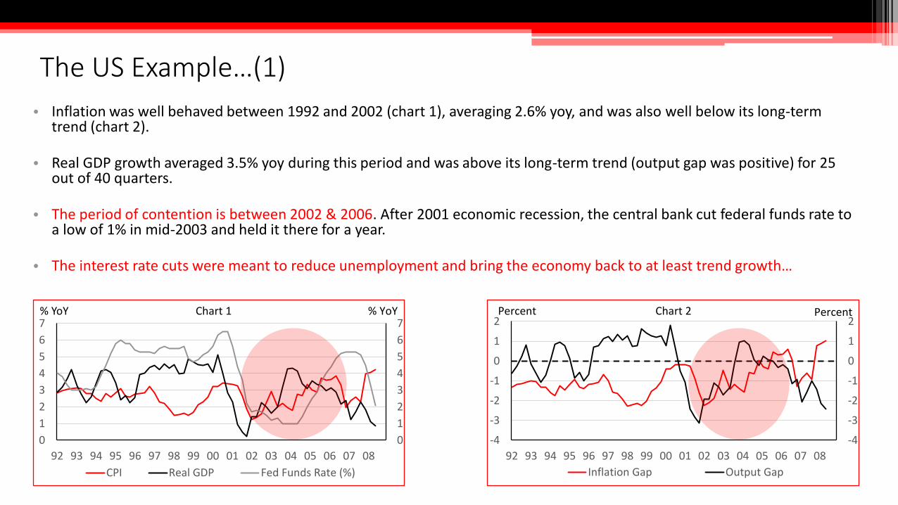
• Inflation was well behaved between 1992 and 2002 (chart 1), averaging 2.6% yoy, and was also well below its long-term trend (chart 2).

• Real GDP growth averaged 3.5% yoy during this period and was above its long-term trend (output gap was positive) for 25 out of 40 quarters.

• The period of contention is between 2002 & 2006. After 2001 economic recession, the central bank cut federal funds rate to a low of 1% in mid-2003 and held it there for a year.

• The interest rate cuts were meant to reduce unemployment and bring the economy back to at least trend growth…

The US Example…(1)

0

1

2

3

4

5

6

7

0

1

2

3

4

5

6

7

92 93 94 95 96 97 98 99 00 01 02 03 04 05 06 07 08

CPI Real GDP Fed Funds Rate (%)

% YoYChart 1% YoY

-4

-3

-2

-1

0

1

2

-4

-3

-2

-1

0

1

2

92 93 94 95 96 97 98 99 00 01 02 03 04 05 06 07 08

Inflation Gap Output Gap

PercentPercent Chart 2

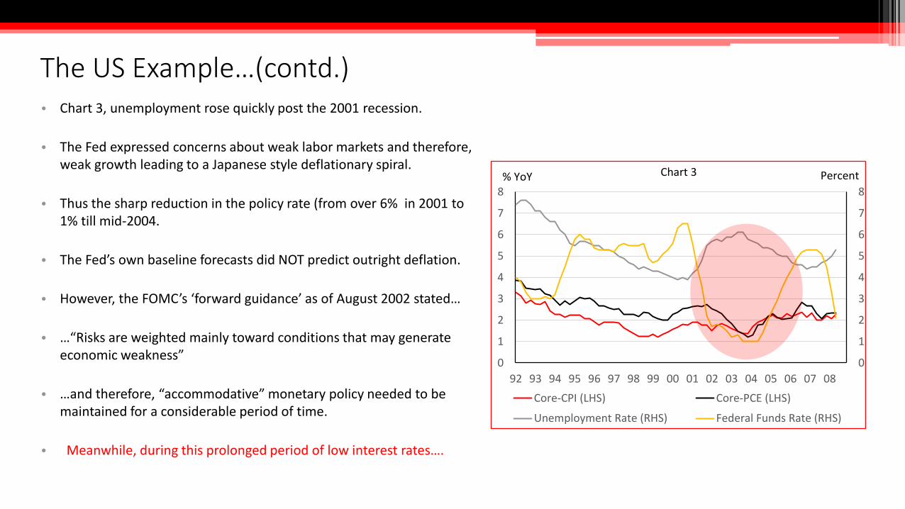
• Chart 3, unemployment rose quickly post the 2001 recession.

• The Fed expressed concerns about weak labor markets and therefore, weak growth leading to a Japanese style deflationary spiral.

• Thus the sharp reduction in the policy rate (from over 6% in 2001 to 1% till mid-2004.

• The Fed’s own baseline forecasts did NOT predict outright deflation.

• However, the FOMC’s ‘forward guidance’ as of August 2002 stated…

• …“Risks are weighted mainly toward conditions that may generate economic weakness”

• …and therefore, “accommodative” monetary policy needed to be maintained for a considerable period of time.

• Meanwhile, during this prolonged period of low interest rates….

The US Example…(contd.)

0

1

2

3

4

5

6

7

8

0

1

2

3

4

5

6

7

8

92 93 94 95 96 97 98 99 00 01 02 03 04 05 06 07 08

Core-CPI (LHS) Core-PCE (LHS)

Unemployment Rate (RHS) Federal Funds Rate (RHS)

Percent% YoY Chart 3

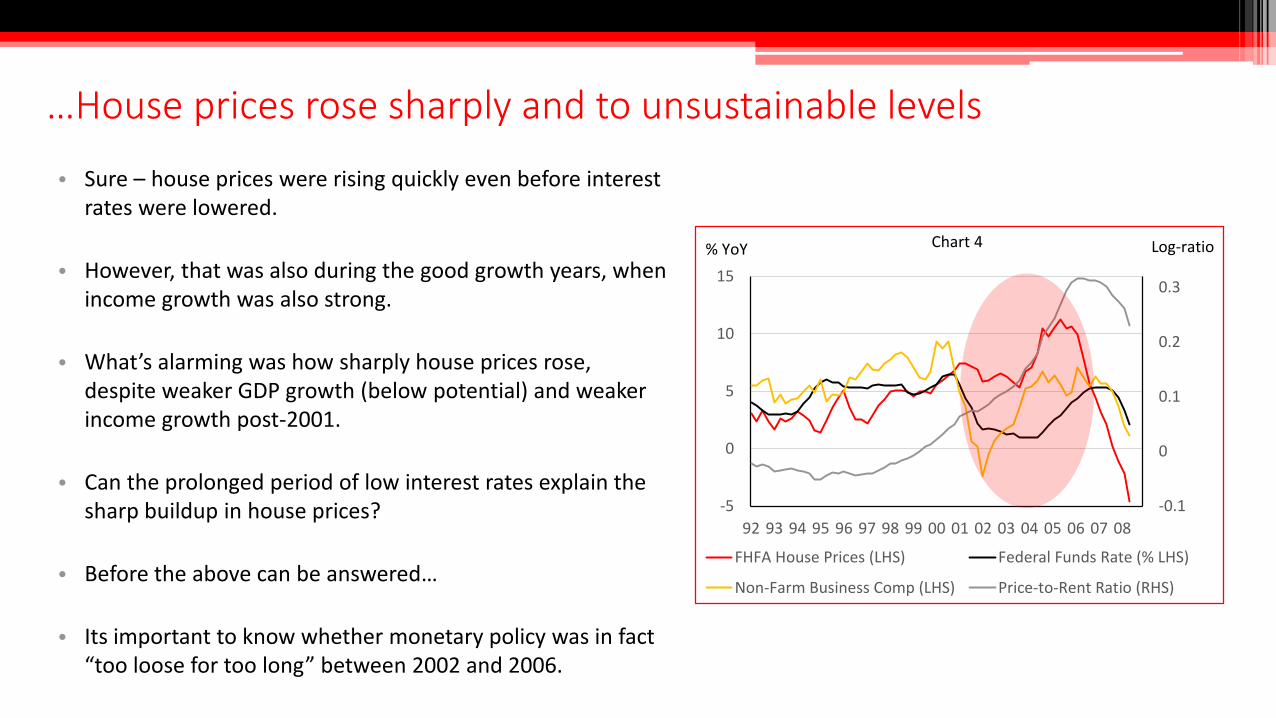
…House prices rose sharply and to unsustainable levels

• Sure – house prices were rising quickly even before interest rates were lowered.

• However, that was also during the good growth years, when income growth was also strong.

• What’s alarming was how sharply house prices rose, despite weaker GDP growth (below potential) and weaker income growth post-2001.

• Can the prolonged period of low interest rates explain the sharp buildup in house prices?

• Before the above can be answered…

• Its important to know whether monetary policy was in fact “too loose for too long” between 2002 and 2006.

-0.1

0

0.1

0.2

0.3

-5

0

5

10

15

92 93 94 95 96 97 98 99 00 01 02 03 04 05 06 07 08

FHFA House Prices (LHS) Federal Funds Rate (% LHS)

Non-Farm Business Comp (LHS) Price-to-Rent Ratio (RHS)

Log-ratio% YoY Chart 4

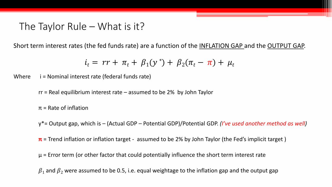
Short term interest rates (the fed funds rate) are a function of the INFLATION GAP and the OUTPUT GAP.

𝑖𝑡 = 𝑟𝑟 + 𝜋𝑡 + 𝛽1(𝑦∗) + 𝛽2(𝜋𝑡 − 𝜋) + 𝜇𝑡

The Taylor Rule – What is it?

Where i = Nominal interest rate (federal funds rate)

rr = Real equilibrium interest rate – assumed to be 2% by John Taylor

π = Rate of inflation

y*= Output gap, which is – (Actual GDP – Potential GDP)/Potential GDP. (I’ve used another method as well)

π = Trend inflation or inflation target - assumed to be 2% by John Taylor (the Fed’s implicit target )

µ = Error term (or other factor that could potentially influence the short term interest rate

𝛽1 and 𝛽2 were assumed to be 0.5, i.e. equal weightage to the inflation gap and the output gap

The Taylor Rule (TR) – What does it imply?

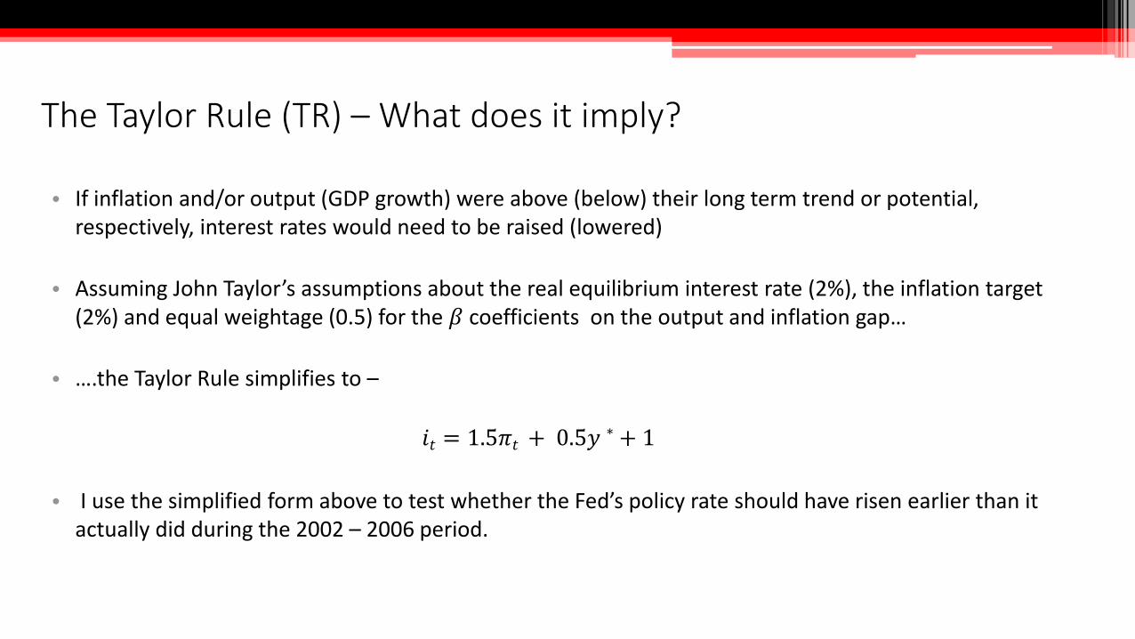
• If inflation and/or output (GDP growth) were above (below) their long term trend or potential, respectively, interest rates would need to be raised (lowered)

• Assuming John Taylor’s assumptions about the real equilibrium interest rate (2%), the inflation target (2%) and equal weightage (0.5) for the 𝛽 coefficients on the output and inflation gap…

• ….the Taylor Rule simplifies to –

𝑖𝑡 = 1.5𝜋𝑡 + 0.5𝑦 ∗ + 1

• I use the simplified form above to test whether the Fed’s policy rate should have risen earlier than it actually did during the 2002 – 2006 period.

TR Results – Should the policy rate have risen sooner?

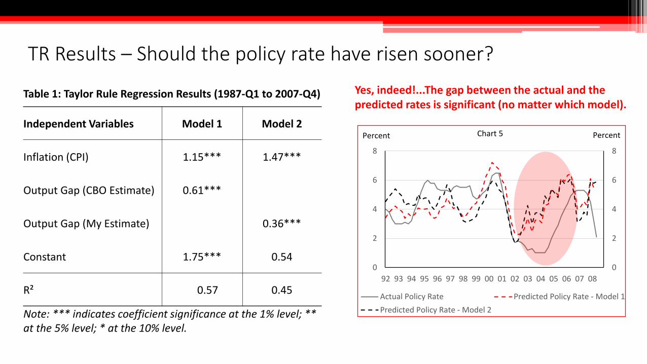
Table 1: Taylor Rule Regression Results (1987-Q1 to 2007-Q4)

Independent Variables Model 1 Model 2

Inflation (CPI) 1.15*** 1.47***

Output Gap (CBO Estimate) 0.61***

Output Gap (My Estimate) 0.36***

Constant 1.75*** 0.54

R² 0.57 0.45

Note: *** indicates coefficient significance at the 1% level; ** at the 5% level; * at the 10% level.

0

2

4

6

8

0

2

4

6

8

92 93 94 95 96 97 98 99 00 01 02 03 04 05 06 07 08

Actual Policy Rate Predicted Policy Rate - Model 1

Predicted Policy Rate - Model 2

PercentPercent Chart 5

Yes, indeed!...The gap between the actual and the predicted rates is significant (no matter which model).

Deviations from TR: The Impact on Housing Market

y = -0.0519x + 0.0633R² = 0.4878

-0.1

0.0

0.1

0.2

0.3

-4 -2 0 2 4

Pri

ce t

o R

ent

Rat

io

Deviations from Taylor Rule – (4th Lag)

Chart 6 – Model 1

y = -0.0351x + 0.061R² = 0.279

-0.1

0.0

0.1

0.2

0.3

-4 -2 0 2 4

Log

Pri

ce t

o R

ent

Rat

io

Deviations from Taylor Rule – 4th Lag

t-stat = -5.63

Chart 7 – Model 2

t-stat = -8.84

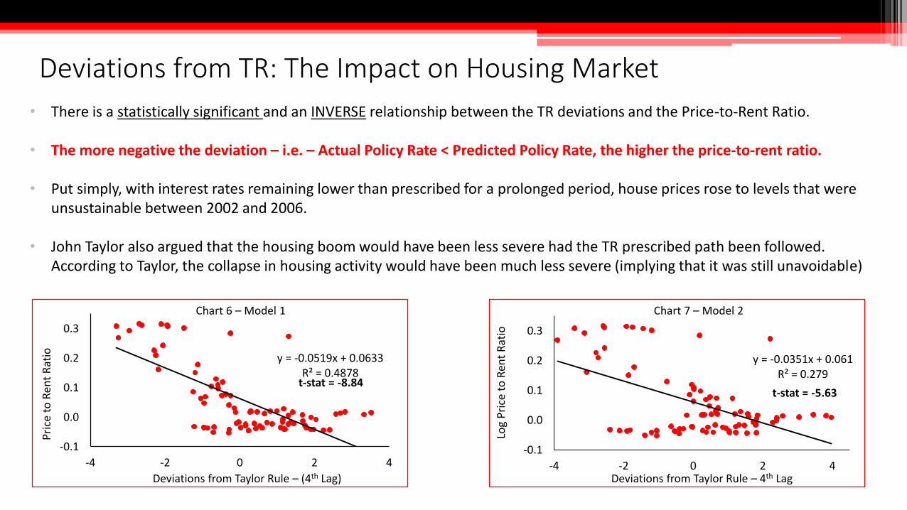
• There is a statistically significant and an INVERSE relationship between the TR deviations and the Price-to-Rent Ratio.

• The more negative the deviation – i.e. – Actual Policy Rate < Predicted Policy Rate, the higher the price-to-rent ratio.

• Put simply, with interest rates remaining lower than prescribed for a prolonged period, house prices rose to levels that wereunsustainable between 2002 and 2006.

• John Taylor also argued that the housing boom would have been less severe had the TR prescribed path been followed. According to Taylor, the collapse in housing activity would have been much less severe (implying that it was still unavoidable)

In Conclusion…

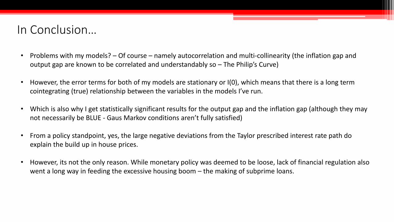
• Problems with my models? – Of course – namely autocorrelation and multi-collinearity (the inflation gap and output gap are known to be correlated and understandably so – The Philip’s Curve)

• However, the error terms for both of my models are stationary or I(0), which means that there is a long term cointegrating (true) relationship between the variables in the models I’ve run.

• Which is also why I get statistically significant results for the output gap and the inflation gap (although they may not necessarily be BLUE - Gaus Markov conditions aren’t fully satisfied)

• From a policy standpoint, yes, the large negative deviations from the Taylor prescribed interest rate path do explain the build up in house prices.

• However, its not the only reason. While monetary policy was deemed to be loose, lack of financial regulation also went a long way in feeding the excessive housing boom – the making of subprime loans.

Thank You