Powered Magnets, DB Formation and Decelerator

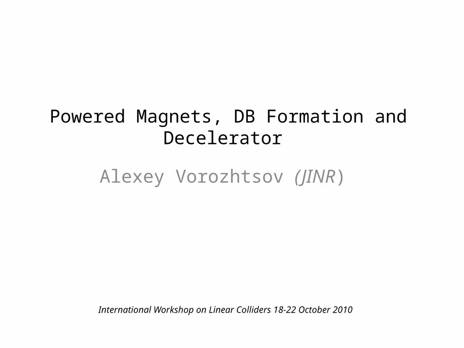
Powered Magnets, DB Formation and Decelerator

Alexey Vorozhtsov (JINR)

International Workshop on Linear Colliders 18-22 October 2010

2

Outline

1. Drive Beam Linac Quadrupole– Requirements and constraints– Initial design– The new “long yoke” proposal– Magnetic field calculations– Field quality– Conclusions

2. Drive Beam magnets for Delay line, Combiner rings, Turn-around, Transport to tunnel, Long transfer line and injector linac– Preliminary electromagnetic design– Cost estimate– Conclusions

Alexey VorozhtsovIWLC10, WG6, 10/20/2010

Alexey Vorozhtsov 3

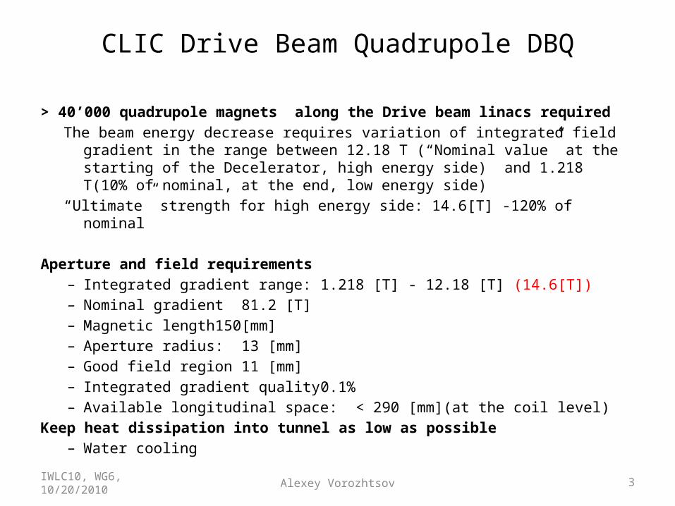
CLIC Drive Beam Quadrupole DBQ

> 40’000 quadrupole magnets along the Drive beam linacs required The beam energy decrease requires variation of integrated field gradient in the range

between 12.18 T (“Nominal value” at the starting of the Decelerator, high energy side) and 1.218 T(10% of nominal, at the end, low energy side)

“Ultimate” strength for high energy side: 14.6[T] -120% of nominal

Aperture and field requirements– Integrated gradient range: 1.218 [T] - 12.18 [T] (14.6[T])– Nominal gradient 81.2 [T]– Magnetic length 150[mm]– Aperture radius: 13 [mm]– Good field region 11 [mm]– Integrated gradient quality 0.1%– Available longitudinal space: < 290 [mm](at the coil level)

Keep heat dissipation into tunnel as low as possible– Water cooling

IWLC10, WG6, 10/20/2010

Alexey Vorozhtsov 4

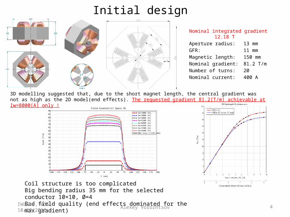
Initial design

200 175 150 125 100 75 50 25 0 25 50 75 100 125 150 175 2000

5

10

15

20

25

30

35

40

45

50

55

60

65

70

75

80

85

90Iw=1000 [A], Iw=3000 [A]Iw=5000 [A]Iw=5500 [A]Iw=6000 [A]Iw=6360 [A]Iw=7500 [A]Iw=9600 [A]DBQ Iron L=138 [mm]

Field Gradient(Z) Opera 3D

Z [mm]

Gra

d [T

/m]

3D modelling suggested that, due to the short magnet length, the central gradient was not as high as the 2D model(end effects). The requested gradient 81.2[T/m] achievable at Iw=8000[A] only !

Nominal integrated gradient 12.18 T

Aperture radius: 13 mmGFR: 11

mmMagnetic length: 150 mmNominal gradient: 81.2 T/mNumber of turns: 20Nominal current: 400 A

Coil structure is too complicatedBig bending radius 35 mm for the selected conductor 10×10, Ø=4Bad field quality (end effects dominated for the max gradient)

IWLC10, WG6, 10/20/2010

Alexey Vorozhtsov 5

New proposal• Increase the iron length(as much as possible taking into account the available space) to

achieve the requested integrated gradient =12.18[T] at smaller current:

][18045.02)()(

][18.12]/[8.62][194]/[2.81][150)0(

mmRbnewLeffnewLiron

TmTmmmTmmGradLeffGL

• Conductor type has been changed from 10×10mm Ø=4mm 20 turns to 6×6 Ø=3.5mm 52 turns=> Smaller bending radius 18mm(smaller total length of the magnet).

IWLC10, WG6, 10/20/2010

Alexey Vorozhtsov 6

2D magnetic field calculations & field quality

11 9 7 5 3 1 1 3 5 7 9 11

8 104

6 104

4 104

2 104

2 104

4 104

6 104

8 104

Gradient 10% of nominalNominal gradientGradient 120% of nominal

Gradient homogeneity of the quadrupole in the horizontal plane

X [mm]

[[G

rad(

x)-G

rad(

0)]

/ Gra

d(0)

]

IWLC10, WG6, 10/20/2010

Alexey Vorozhtsov 7

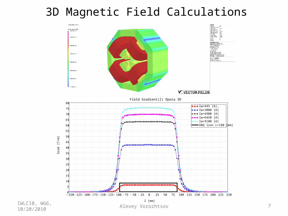
3D Magnetic Field Calculations

250 225 200 175 150 125 100 75 50 25 0 25 50 75 100 125 150 175 200 225 2500

5

10

15

20

25

30

35

40

45

50

55

60

65

70

75

80Iw=445 [A], Iw=3000 [A]Iw=4900 [A]Iw=6450 [A]Iw=9100 [A]DBQ Iron L=180 [mm]

Field Gradient(Z) Opera 3D

Z [mm]

Gra

d [T

/m]

IWLC10, WG6, 10/20/2010

Alexey Vorozhtsov 8

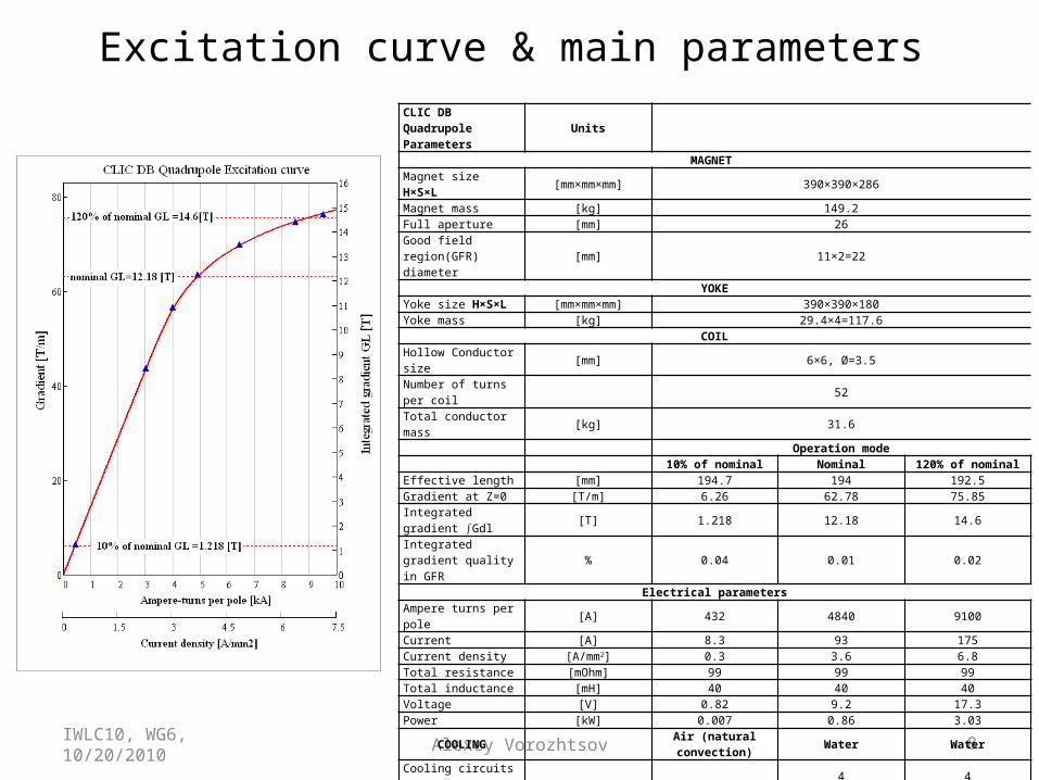
Excitation curve & main parametersCLIC DB Quadrupole Parameters Units

MAGNET Magnet size H×S×L [mm×mm×mm] 390×390×286Magnet mass [kg] 149.2Full aperture [mm] 26

Good field region(GFR) diameter [mm] 11×2=22

YOKEYoke size H×S×L [mm×mm×mm] 390×390×180Yoke mass [kg] 29.4×4=117.6

COIL

Hollow Conductor size [mm] 6×6, Ø=3.5

Number of turns per coil 52

Total conductor mass [kg] 31.6

Operation mode10% of nominal Nominal 120% of nominal

Effective length [mm] 194.7 194 192.5Gradient at Z=0 [T/m] 6.26 62.78 75.85

Integrated gradient ∫Gdl [T] 1.218 12.18 14.6

Integrated gradient quality in GFR % 0.04 0.01 0.02

Electrical parameters

Ampere turns per pole [A] 432 4840 9100

Current [A] 8.3 93 175Current density [A/mm2] 0.3 3.6 6.8Total resistance [mOhm] 99 99 99Total inductance [mH] 40 40 40Voltage [V] 0.82 9.2 17.3Power [kW] 0.007 0.86 3.03

COOLINGAir (natural convection) Water Water

Cooling circuits per magnet 4 4

coolant velocity [m/s] 1.1 1.9

cooling flow per circuit [l/min] 0.6 1.1

Pressure drop [bar] 2.2 5.7Reynolds number 4122 8210Temperature rise [K] 5 10

IWLC10, WG6, 10/20/2010

Alexey Vorozhtsov 9

Field quality 3D for various Integrated gradient values, chamfer 2.5 mm

0 1 2 3 4 5 6 7 8 9 10 110.07

0.05

0.03

0.01

0.01

0.03

0.05

0.07

10% of GL= 1.218 [T]Nominal GL= 12.18 [T]120% of GL= 14.6 [T]

Horizontal distribution of the integrated gradient error [%]

X [mm]

{ G

L(x

)-G

L(0

) }

/ GL

(0)

[%

]B2 B3 B4 B5 B6 B7 B8 B9 B10 B11 B12 B13 B14 B15 B16 B17 B18 B19 B20 B21 B22

Absolute value of the integrated relative field components , chamfer 2.5 [mm]

Iw=445[A] 10% of nominalIw=4900[A] NominalIw=9100[A] 120% of nominal

Harmonic number

abs(

∫Bnd

z/∫B

2dz)

Chamfer height: 2.5mm

IWLC10, WG6, 10/20/2010

Alexey Vorozhtsov 10

Conclusions on DBQ design

• The electromagnetic design of the CLIC DB quadrupole has been presented

• The proposed design fulfill the requirements: Available space, integrated gradient up to 120% of nominal value 12.18[T]

• To study the end field effects the 3D model of the magnet has been constructed

• The 3D field analysis shows that the minimum integrated field error is mandated for the chamfer height 2.5mm and it stays below the requested value 0.1% at GFR=11[mm] for the full range of the integrated field gradient (1.218[T]-14.6 [T]).

IWLC10, WG6, 10/20/2010


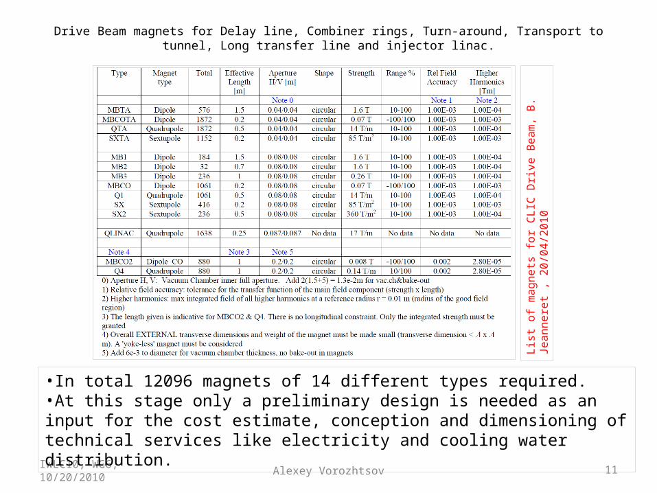
Drive Beam magnets for Delay line, Combiner rings, Turn-around, Transport to tunnel, Long transfer line and injector linac.

IWLC10, WG6, 10/20/2010

•In total 12096 magnets of 14 different types required. •At this stage only a preliminary design is needed as an input for the cost estimate, conception and dimensioning of technical services like electricity and cooling water distribution.

List

of m

agne

ts fo

r CLI

C D

rive

Beam

, B. J

eann

eret

, 20

/04/

2010


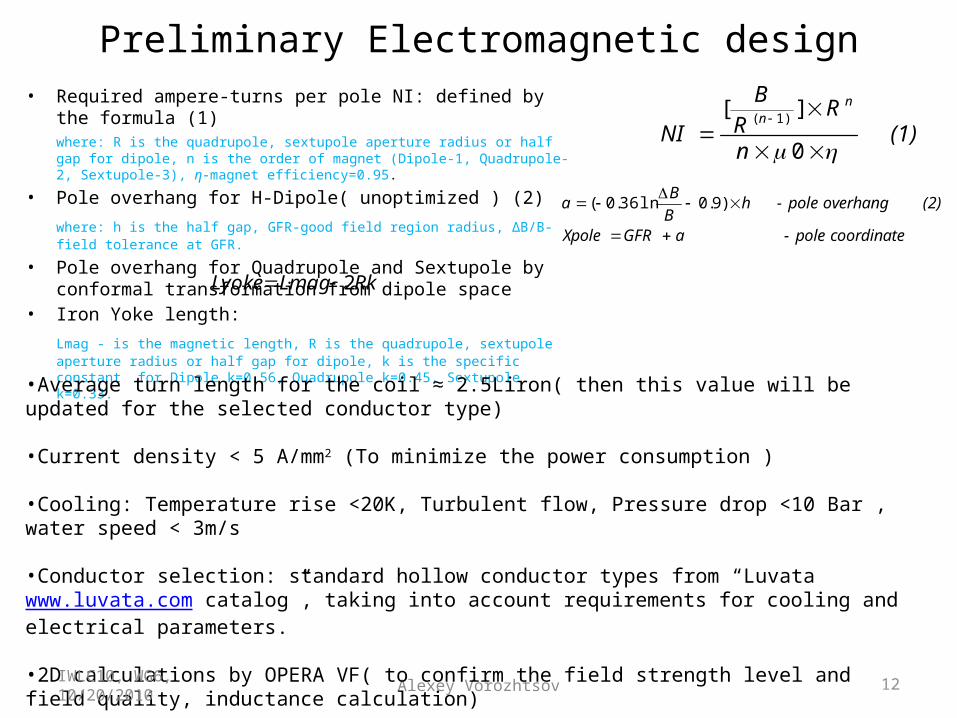
Preliminary Electromagnetic design• Required ampere-turns per pole NI: defined by the formula (1)

where: R is the quadrupole, sextupole aperture radius or half gap for dipole, n is the order of magnet (Dipole-1, Quadrupole-2, Sextupole-3), η-magnet efficiency=0.95.

• Pole overhang for H-Dipole( unoptimized ) (2)

where: h is the half gap, GFR-good field region radius, ∆B/B- field tolerance at GFR.

• Pole overhang for Quadrupole and Sextupole by conformal transformation from dipole space

• Iron Yoke length:

Lmag - is the magnetic length, R is the quadrupole, sextupole aperture radius or half gap for dipole, k is the specific constant for Dipole k=0.56, Quadrupole k=0.45, Sextupole k=0.33.

(1) n

RR

B

NI

nn

0

][ )1(

coordinate pole- aGFRXpole

(2) overhang pole- hB

Ba

)9.0ln36.0(

RkLmagLyoke 2

•Average turn length for the coil ≈ 2.5Liron( then this value will be updated for the selected conductor type)

•Current density < 5 A/mm2 (To minimize the power consumption )

•Cooling: Temperature rise <20K, Turbulent flow, Pressure drop <10 Bar , water speed < 3m/s

•Conductor selection: standard hollow conductor types from “Luvata www.luvata.com catalog”, taking into account requirements for cooling and electrical parameters. •2D calculations by OPERA VF( to confirm the field strength level and field quality, inductance calculation)

•Table with the main parameters

IWLC10, WG6, 10/20/2010

http://www.luvata.com/


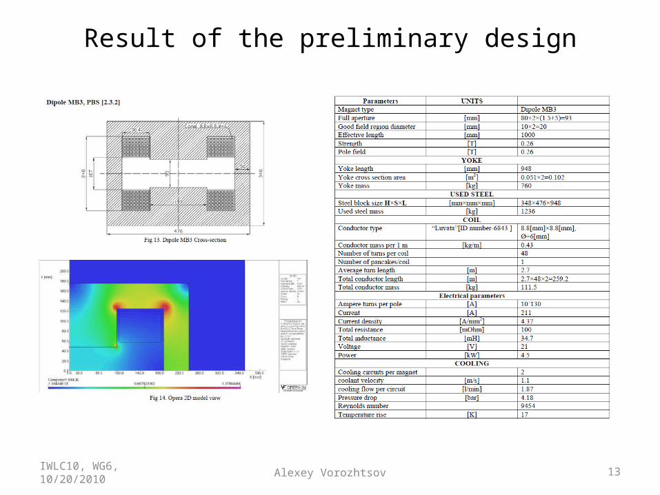
Result of the preliminary design

IWLC10, WG6, 10/20/2010


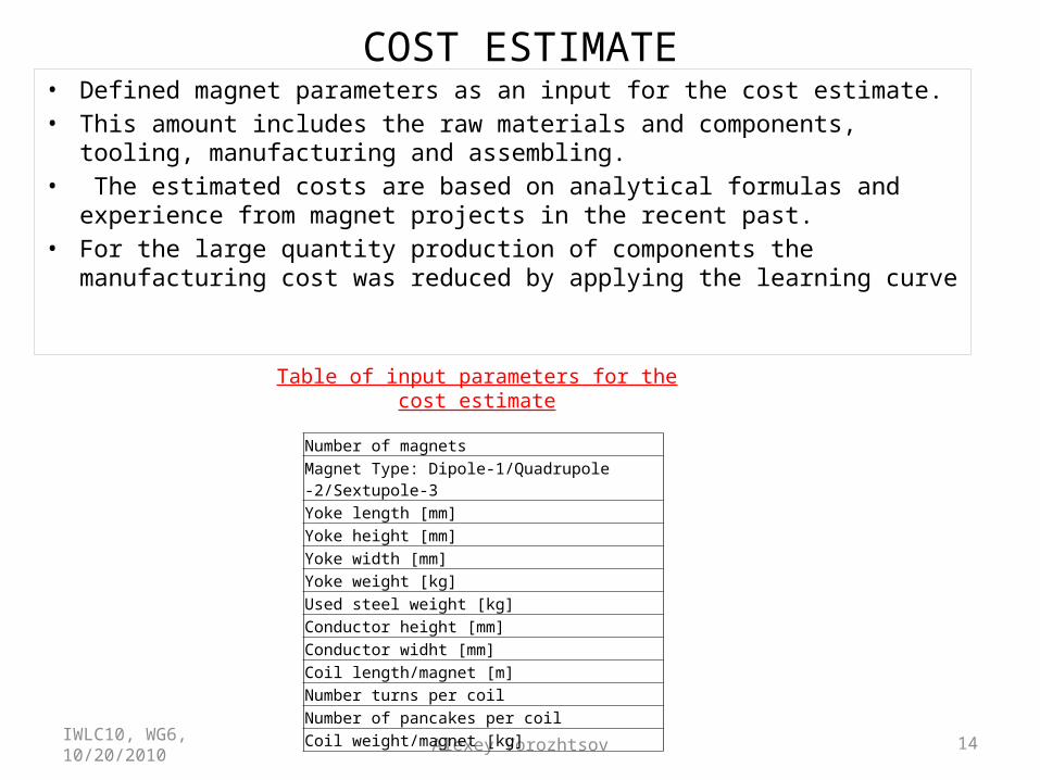
COST ESTIMATE• Defined magnet parameters as an input for the cost estimate. • This amount includes the raw materials and components, tooling,

manufacturing and assembling.• The estimated costs are based on analytical formulas and experience from

magnet projects in the recent past.• For the large quantity production of components the manufacturing cost was

reduced by applying the learning curve

Number of magnetsMagnet Type: Dipole-1/Quadrupole -2/Sextupole-3Yoke length [mm]Yoke height [mm]Yoke width [mm]Yoke weight [kg]Used steel weight [kg]Conductor height [mm]Conductor widht [mm]Coil length/magnet [m]Number turns per coil Number of pancakes per coilCoil weight/magnet [kg]

Table of input parameters for the cost estimate

IWLC10, WG6, 10/20/2010


Cost estimate• Material:

– Steel sheets(used steel mass) : 2 CHF/kg– Copper conductor( conductor mass): 20 CHF/kg

• Fixed cost– Punching die (yoke cross section)– Stacking tool (yoke mass) – Winding (turn length)– Molding (coil volume)

• Manufacturing cost– Yoke manufacturing (Yoke mass/Yoke parts)– Coil manufacturing(One Coil mass)

• Assembling(Magnet mass)• Learning curve(for big series):

0 1 2 3 4 5 6 7 8 9 10 11 12 13 14 15 16 17 18 19 201

10

100Yoke manufacturing cost(weight of 1 yoke part) [kCHF]

1 part yoke weight [tons]

Yok

e M

anuf

actu

ring

Cos

t [kC

HF

]

0 50 100 150 200 250 300 350 400 450 500 550 600 650 700 750 800 850 900 950 10001

10

100COIL manufacturing cost(coil weight) [kCHF]

1 coil weight [kg]C

OIL

Man

ufac

turi

ng C

ost [

kCH

F]

produced units n first of cost unit Average- C(n)/n

units n first of cost cumulative- nC

nCa

a

)log1(

)]1([)(

2

log1 2

IWLC10, WG6, 10/20/2010


Conclusions

Type Magnet type

Number of magnets

COST(1st Magnet) [kCHF]

COST(Average unit) [kCHF]

Power consumption [kW]

Per magnet TOTAL Per

magnet TOTAL Per magnet TOTAL

MBTA Dipole 576 21.6 12441.6

MBCOTA Dipole 1872 0.25 468

QTA Quadrupole 1872 2 3744

SXTA Sextupole 1152 0.075 86.4

MB1 Dipole 184 42 7728

MB2 Dipole 32 25 800

MB3 Dipole 236 4.5 1062

MBCO Dipole 1061 0.4 424.4

Q1 Quadrupole 1061 5.9 6259.9

SX Sextupole 416 0.5 208

SX2 Sextupole 236 3.3 778.8

QLINAC Quadrupole 1638 6.3 10319.4

MBCO2 Dipole 880 0.313 275.44

Q4 Quadrupole 880 0.543 477.84

TOTAL 12096 45073.78

•Preliminary design and cost estimate of the CLIC Drive Beam magnets has been completed.

•In total 12096 magnets of 14 different types have been considered.

•The total power consumption of all magnets is about 45MW.

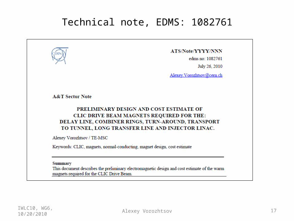
EDMS document №1082761

IWLC10, WG6, 10/20/2010


Technical note, EDMS: 1082761

IWLC10, WG6, 10/20/2010


AcknowledgmentI would like to express my gratitude to Davide Tommasini, Michele Modena and Bernard Jeanneret for their help and useful discussion.

References

1. E. Adli. Draft Drive Beam Decelerator Magnet Specification, EDMS no 9927902. B. Jeanneret. List of magnets for the CLIC Drive Beam, Internal note, 2010-04-20.3. D. Schulte. List of Magnet Requirements for CLIC. EDMS no 1000727, 2010-06-074. Ph. Lebrun. Issues, methods and organization for costing the CLIC accelerator

project. Special BDS-MDI meeting, CERN 2010-06-2010

IWLC10, WG6, 10/20/2010

Documents

Powered Magnets, DB Formation and Decelerator