Power spectrum of wind-influenced vegetation backscatter at X-band

R.M. Narayanan D.W. Doerr D.C. Rundquist

Indexing t e r m : Radar, Power spectrum, Vegetation, Clutter

Abstract: The baseband power spectral density characteristics of X-band radar backscatter from wind-influenced vegetation were investigated using a short-range continuous wave radar system. Radar reflectance and concurrent wind- speed data were gathered from various individual trees from a distance of approximately 30 m. The power spectral density was observed to drop off at a rate slower than the widely-used single-peak Gaussian model. An empirical model which char- acterises the power spectrum as a combination of Gaussian functions with different peak locations is proposed. The model postulates that (i) the spec- tral broadening of the central peak is attributable to branch sway, (ii) the location of non-central peaks is attributable to leaf flutter, and (iii) the spectral broadening of the non-central peaks is attributable to a combination of branch sway and leaf flutter. The model shows satisfactory agree- ment with measured data. It is shown that realistic estimates of MTI improvement factors for delay- line cancellers can be obtained by knowledge of the type of vegetative clutter environment.

1 Introduct ion

The scattering properties of vegetated surfaces are of interest in various types of radar and remote sensing system applications. Since vegetated targets can be viewed as a collection of many elementary scatterers, radar signals scattered from such targets fluctuate ran- domly as their orientations change due to wind action, resulting in spectral broadening of the baseband signal. Although the spectrum is related to the velocities of the scatterers within the resolution cell, the spectral widths do not exactly scale with the operating frequency. It has been established that the spectral broadening is in fact attributable to more than one source of fluctuation, and an accurate knowledge of the spectral characteristics can provide improved and possibly near-optimum detection of moving targets in vegetative clutter environments.

0 IEE, 1994 Paper 9893F (E15), first received 20th July 1992 and in revised form 30th April 1993 R.M. Narayanan and D.W. Doerr are with the Department of Electrical EngineringKenter for Electro-optics, University of Nebraska, Lincoln, NE 68588, USA D.C. Rundquist is with the Center for Advanced Land Management Information Technologies, University of Nebraska, Lincoln, NE 68588, USA

I E E Proc-Radar, Sonar Navig., Vol . 141, No. 2, April IYY4

To understand the power spectral density character- istics of vegetated targets under the influence of the wind, various theoretical and experimental studies have been carried out by researchers. The theoretical models con- sidered the general case of vibrating and oscillating ensemble of scatterers to model vegetation under the influence of wind, while empirical models derived from experimental studies had the drawback of not being physically based. Extension of both types of models to individual trees under specific windspeed conditions was not practicable.

Our approach has concentrated on applying a specific theoretical model, suitably modified so as to possess physical relevance, to extensive data gathered from indi- vidual trees using a short-range X-band continuous wave (CW) radar system. The empirical model so derived appears to agree with data gathered from both coniferous and deciduous trees reasonably well over a wide range of windspeeds.

2 Experimental setup

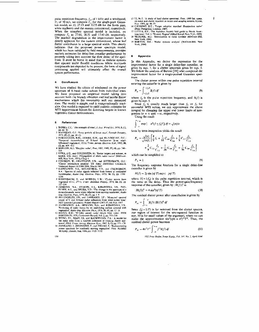
2.1 Radar system overview The block diagram of the radar system used in the study is shown in Fig. 1, while its relevant specifications are summarised in Table 1. The H P 8720A network analyser Table 1 : Speci f icat ions of t h e radar s y s t e m

Tvoe Continuous wave

Frequency 8 GHz Power output 10 mW IF bandwidth 3 kHz Dynamic range 70 dB Antenna beamwidth 3.5 deg. Polarisation Vertical transmit

Positionina Azimuth and elevation Vertical receive

operates between 130 MHz and 20 GHz; for our studies, the operating frequency was set at 8 GHz. The H P 8349B amplifier was used to provide a transmit power of 10 mW. Both transmit and receive antennas had a beam- width of 3.5" at 8 GHz, which resulted in a spot size of

The equipment used in this study was funded by a grant from the National Science Foundation. We appreciate the valuable comments and suggestions made by Dr. David K. Barton, Dr. Maurice W. Long, and Dr. Merrill I. Skolnik which greatly improved the content and readability of this

125

1.8 m on tree crown when viewed from a distance of 30m. The 2D2/1 far field distance of the antennas was computed as 20 m. Isolation between the antennas was

size of 1.8 m, so that the spot was well-contained within the tree crown. We estimate the correlation distance of the wind to be greater than the 30 m separation between

transmit ontenna HP9153C

hard disc HP8720A port 1 HP8349B microwove network port 2

amplifier -+ :- onolyser

Fig. 1 Block diagram of radar system

improved by using a metallic shield between them. The metallic shield was adjusted so that the power leaking into the receiver from the transmitter when the two antennas were pointing up into the sky was of the order of the receiver noise floor. The polarisation combination used was VV, i.e. vertical transmit and vertical receive. Although no measurements were made for HH (horizontal transmit and horizontal receive) polarisation, we expect those results to be similar to the VV case since the branches and leaves assumed inclination angles that ranged from near-vertical to near-horizontal under the influence of the wind. Antennas were mounted on top of a van, viewing the tree targets horizontally, while the electronic equipment and computers were housed within the van. Windspeed was monitored using a Met One 014A anemometer, which was computer-controlled to record data at exactly the same time as the radar meas- urement. The windspeed sensor was mounted on a 5 m high mast attached on the roof of the van, and care was taken to ensure that the air flow to the sensor was not blocked by the antennas. Although the wind direction was not monitored, we conjecture the high windspeeds cause a more uniform motion of the tree constituents that is expected to be fairly independent of the wind direction.

22 Characteristics of trees studied A list of individual, isolated trees that were studied is provided in Table 2. As can be noted, the crown diameter of each tree was much larger than the illuminated spot

receive antenna

the tree and the windspeed sensor, owing to the absence of any protuberances at the test site. The trees chosen for the study showed considerable variability in their response to wind action. Leaf or needle flutter depends largely on the stiffness of leafstalks or needles, and to some extent on branch stiffness [l], while branch vibra- tion depends primarily on branch stiffness [2].

3 Power spectral density characteristics

3.1 Experimental observations The radar backscattered power was recorded from each tree over a 5 s duration. Approximately 1600 power samples were obtained at intervals of 3.125 ms. Since the typical decorrelation time during moderate windspeeds (> 7.5 m/s) when the tree is generally in uniform motion was measured to be approximately 50 ms [3], the obser- vation time was greater than the typical decorrelation time by a factor of over 100. This ensured that accurate spectral information was obtained by allowing the time series to develop fully. From the radar reflectance data, autocovariance plots were generated as a function of time lag, which were then Fourier transformed to yield the power spectrum. As expected, for each tree type, the base- band power spectral density curves broadened as wind- speed increased. Typical spectra for various individual trees under low and moderate windspeed conditions are shown in Figs. 2-5. These Figures have been specifically chosen to illustrate the wind response of typical tree

Table 2: Physical characteristics of trees investigated

Tree Tree name Height, Trunk Crown Branches Leafstalks m diameter, diameter, or twigs or needles

m m

01 02 03 04 05 06 07 08 09 10 11 12 13 15 16

Austrian pine Scots pine Scots pine Eastern cottonwood Scots pine Scots pine Scots pine

Eastern black walnut Siberian elm Siberian elm White mulberry White mulberry Oaks Eastern cottonwood

Apple

6 0.33 8 0.35 8 0.23

16 0.48 10 0.53 8 0.72

19 0.55 5 0.67

12 0.55 16 0.62 13 (av.) 0.29 (av.) 10 0.82 12 (av.) 0.56 (av.) 15 (av.) 0.49 (av.)

9 0.50

6 7 7 9

12 11 11 8

14 12 15 group 16 14 group 18 group 8

stout stout stout stout stout stout stout stout stout slender slender slender slender

stout -

stiff stiff stiff slender stiff stiff stiff stiff stalkless stiff stiff stiff stiff

slender -

126 I E E Proc.-Radar, Sonar Navig., Vol. 141, No. 2, Aprd 1994

structures such as the Scots pine (coniferous tree with stiff needles and stout branches), eastern black walnut (deciduous stalkless tree with stout branches), white mul-

0 -

-10

2 - 2 0 - ; o--30 U)

-40

teristics. Furthermore, higher windspeeds cause wider spectra, and are therefore harsher clutter environments for moving target detection, and consequently we have

-

-

-

Fig. 2 frequency, Hz

Measured power spectral density characteristics of Scots U = 1.9 m/s U = 8.4 mis

pine

-501 I I I I I I I -10 0 20 40 60

frequency, Hz

Fig. 3 black walnut ....... U = 2.5 ~ U = 7.8 m/s

Measured power spectrnl density characteristics of eastern

20 40 6 0 - 5 O L I I I I ' I

-10 0 frequency, Hz

Fig. 4 Measured power spectral density characteristics of white mulberry

U = 1 t m/s ~ U = 7.9 mls

berry (deciduous tree with stiff leafstalks and slender branches) and eastern cottonwood (deciduous tree with slender leafstalks and stout branches). There appeared to be larger variations in the shape and the spectral width for the same tree under low windspeed conditions (i 5 m/s), presumably because the movement of the branches and leaves were not really uniform, and also because the motion of the tree was highly dependent on the wind direction. At moderate windspeeds (> 7.5 m/s), the branches and leaves were generally in uniform motion, resulting in less variability in the spectral charac-

.......

I E E Floc.-Radar, Sonar Nauiy., Vol . 141, No . 2, April 1994

- 3 0 1

20 40 60 -35L ' ' I ' ' '

-10 0 frequency. Hz

Fig. 6 cottonwood ....... U = 3.7 m{s

~ U = 7.5 m/s

modelled and analysed the spectra under moderate wind- speed conditions.

3 2 Survey of earlier investigations Power spectral density studies of vegetation have been the subject of numerous past investigations. The earliest investigations postulated a Gaussian model, centred at zero frequency, which appeared to fit the measured power spectrum of various types of fluctuating targets at L-band [4]. However, the Gaussian model was not suc- cessful in explaining observed anomalous behaviour that showed slower rate of decay at higher frequencies, prob- ably on account of two or more scattering mechanisms [SI. Various types of power law models, with exponents ranging from -3 to - 6 depending upon the terrain and/or windspeed, and decaying at rates slower than the Gaussian model, were found to fit measured data at UHF, L-band and X-band frequencies [6-91. An exponential decay model has also been proposed for the tail region of the power spectrum on the basis of mea- sured clutter data at L and X-bands [lo], while a com- bination of an exponential model for frequencies close to the carrier and a power law with exponent between -2.6 and - 5.8 at frequencies far removed from the carrier was observed for individual tree species [ll]. The power spec- trum of millimetre wave vegetative clutter showed a com- bination of two power law models, each with an exponent of - 2 but with a different half-power frequency c121.

First-principle models that derive the power spectral density function resulting from two independent fluctua- tion mechanisms have also been proposed [13, 141, that yield good agreement with measured data. A detailed comparison between the model developed by Wong, Reed and Kaprielian [13] and various types of power law models with different exponent values showed that the Wong model did indeed closely match the power law models that were derived from measured data [l5]. Wong's model also explained the mechanics of occurrence of the high-frequency components in the spec- trum as windspeed, and hence, scatterer oscillation increased. Our own study also confirmed the applicabil- ity of the Wong model, suitably modified, to measured radar clutter decorrelation phenomena of individual trees

Measured power spectral density characteristics of eastern

c31.

I L l

3.3 Proposed power spectrum model The starting point for our model is the expression for the autocovariance function R(T) of a rotating ensemble of scatterers, derived by Wong et al., for VV backscatter, i.e.

R(r) = exp [~u:~’]

where ud is the Doppler frequency standard deviation, W, is the mean random rotation frequency and U, is the stan- dard deviation of the random rotation frequency. All of the above quantities, viz. udr 0, and nr are expressed in radians per second. When we applied the above model to the measured autocovariance function from individual trees, we assumed that

(i) The Doppler frequency standard deviation was a result of branch vibration and is proportional to the windspeed, U, i.e. ud = C,U

(ii) The mean random rotation frequency was a result of leaf flutter, and is proportional to the windspeed, U, i.e. Ts; = C, U

(iii) The standard deviation of the rotation frequency was zero, i.e. all leaves flutter at the same frequency

Thus

where C, and C, are characteristic constants for each tree, that are obtained from least-squared fit of the model to the measured data. These constants are shown in Table 3 for selected trees that were investigated for their power spectral density characteristics.

The power spectrum S(f) is obtained by taking the Fourier transform of R(T) as

2 (1+f2I2 +-PI- 9 f: }

1 36

+ - 1 exp { - +}] (f + 2f 36 (3)

where f, = C,U/n and fi = C, U/n. The value of S(f) at 1 = 0 is given by

+‘exp{-$}] 18

Although the above model was quite simple and agreed reasonably well with the measured autocovariance data

Tree Tree e,. e,. e,. Table 3: Constants C,, C, and C, for selected trees

code name radlm rad/m rad/m

03 Scatspine 2.5 1.3 2.55 08 Apple 0.7 1.6 1.95 09 Eastern black walnut 1.2 1.7 2.3 10 Siberian elm 2.5 1.1 2.35 13 White mulberry 4.4 1.1 3.3 16 Easterncottonwood 2.1 7.2 8.25

128

131, it did not fit very well the observed power spectrum, especially at frequencies far removed from the carrier. It was observed that the assumed model decayed much faster than the measured data, and this indicated that perhaps the basic assumptions of the model needed to be revised. One such assumption was that all leaves flutter at the same frequency. However, if the standard deviation of the rotation frequency, U,, is assumed not to be zero, but also proportional to the windspeed, U, i.e. U, = C, U, then better agreement was obtained by properly choosing the value of C, .

For nonzero C, , eqn. 1 becomes

R(T) exp [ - C: U2r2]

2 c:,(f -f2I2 + - 9 c,, exp { - T} + - 2 c,, exp { - T} C L ( f + f 2 I 2

+-c,,exp{- 1 c:,u; f l 2f#}

9

36

where Cl2 and C,, are defined as

Cl JCc: + 4 c 3

C - and C,, = - J(C: + 2 ~ : )

S(0) is then simplified as

1 18

Note that in the above equations, the terms C,, and C,, are both less than 1.

Eqn. 5 indicates that the power spectrum of vegetative backscatter consists of Gaussian functions centred at f = 0, f = f2 and f = 2f2 whose spectral widths are some weighted functions off,. Since fi = C,U/rr and f2 = C,U/n, it follows that the spectral widths depend on branch vibration (via C,), while the locations of the peaks depend on leaf flutter (via C,). We also recognise that f, and f2 are in reality twice the branch vibration frequency and leaf flutter frequency in hertz, respectively. Further- more, the ‘tail’ of the power spectrum at frequencies far removed from the carrier is primarily due to the large spectral width of the last four terms, each of which is larger than the spectral width of the first central peak. Observe that the spectral width (defined as the frequency deviation around the centre frequency where the ampli- tude of the Gaussian function attains a value of l/e) is f,,

six terms within the square brackets in eqn. 5, respect- ively, and that the last five spectral widths are greater

fllC14, f l lC12, fi/Ci2, fl/C14 and fllC14 for each of the

I E E Proc.-Radar, Sonar Nouig., Vol. 141, No. 2, April I994

than the first value, viz. f,, since C,, and C,, are both less than 1.

Two questions arise: (i) ‘What is the value of C, (assumed to be zero in our prior analysis)? and (ii) ‘How does a nonzero value of C, affect our prior results?

To answer the first question, we recognise that C3 is related to the standard deviation of the leaf flutter fre- quency. A careful examination of the motion of vegeta- tive constituents under wind action indicates that the above standard deviation is related to both the mean leaf flutter frequency ( f2/2 = C, U/24 and the branch vibra- tion frequency (fJ2 = ClU/2x). Even if the leaf does not flutter by itself, there is some momentum transferred to it by the vibrating branch to which it is connected. We note that the ratio of the frequency of leaf flutter to that of the branch vibration is given by C,/C, . For the Scots pine tree, this ratio is computed as 0.52. A study carried out to classify vegetation based on adaptive radar illumination indicated that the above ratio was approximately 1.5 for pine, 1.0 for spruce, and 5.0 for birch [16]. Although C , and C, values are not available for the birch tree, it is similar in structure to the white mulberry, in that it has slender branches and stiff leafstalks 1171. Thus, its spec- tral characteristics are expected to be qualitatively similar to the white mulberry. For the white mulberry, the ratio of leaf flutter to branch vibration frequency based on the C,/C, ratio is computed as 0.25. Since corresponding ratios in Reference 16 are much higher (and greater than I), it is clear that C, is nonzero, and can reasonably be approximated by some linear combination of C, and C, . The best fits to the power spectral curves were obtained by assuming

(6) C 2

c, = c, + 2

for both coniferous and deciduous trees. Plots of measured and computed power spectra for

typical trees are shown in Figs. 6a-c. Reasonable agree- ment, especially at the tail of the spectra, is seen between the model and the data. Similar agreement was obtained for the other trees listed in Table 3. We have purposely not quantified the goodness of fit by computing, say, the root-mean-squared error between the model and data. It is to be recognised that although various factors are involved in accurately modeling the power spectrum, our model gives qualitative agreement with trends in the measured data using simple best-fit parameters obtained from physical principles. We note that C, is 2.55 for the

Scots pine, 3.3 for the white mulberry and 8.25 for the cottonwood. The values for C,, Cz and C , are seen to possess some physical significance. At a windspeed of 10 m/s, the branch vibration frequency, the mean leaf/ needle flutter frequency and the flutter frequency stand- ard deviation are computed as 4.0, 2.1 and 4.1 Hz, respectively, for the Scots pine, 7.0, 1.8 and 5.3 Hz, respectively, for the white mulberry, and 3.3, 11.4 and 13.1 Hz, respectively, for the eastern cottonwood. These values appear quite reasonable, and provide the justifica- tion for the above choice of C,, C, and C, values. Table 3 also shows C, values for the trees investigated, as obtained from eqn. 6.

As mentioned earlier, we need to reconcile the nonzero value of C, with our earlier results, From the eqns. 2 and 4, it is noted that the major contributor to the decay of the autocovariance function at large time lags is the multiplicative exponential term, viz. exp { - C ~ U ~ Z ~ } . Thus, to a large extent, C, determines the shape of R(z), which is not very sensitive to the choice of C, . Thus, our earlier results are not violated as far as the general auto- covariance function is concerned. Assuming C, = 0 does not largely alter the shape of the autocovariance curve. This is also seen from the fact that a value of C, = 0 does indeed fit the spectra close to the carrier, but a nonzero value of C , is, however, necessary to obtain agreement between model and data at frequencies far removed.

3.4 Application to MTI system performance We extend our above result to obtain some realistic estimates for the MTI improvement factor for the single delay-line canceller. For a single-peak Gaussian clutter spectrum centred at zero frequency with spectral width fl, the improvement factor, I,, has been computed as C181

where f, is the pulse repetition frequency. The above expression was derived by assuming that the clutter spec- tral width is much smaller than the pulse repetition fre- quency. For the case when the power spectrum is of the form given by eqn. 5rwe can show that the improvement factor, I’l, can be expressed as (see Appendix)

(7) 1 4 cz

I; = f +f :[; (1 + + &) + j <] For C, = 0, and C, = 0, i.e. for the single-peak Gaussian model, we verify that 1; does indeed reduce to I,. For a

oc -L

5 % -30 U -20

6 - 4 0

a -50 V

frequency, Hz frequency, Hz frequency, Hz a b C

Fig. 6 a Scots pine: windspced 8 4 m/s b White mulberry: windspeed 7.9 mJs c Eastern cottonwood: windspeed 7.5 mJs The computed curve uses eqns. 5 and 6

measured PSD ~ wmputedPSD

Measured and computed power spectral density characteristics

. . . . . . .

I E E Proc.-Radar, Sonar Nnvig., Vol. 141, No. 2, April 1994 129

pulse repetition frequency, f,, of 1 kHz and a windspeed, U, of 10 m/s, we compute I,, for the single-peak Gauss- ian model, as 32, 27.13 and 33.55 dB for the Scots pine, white mulberry and the eastern cottonwood, respectively. When the complete spectral model is included, we compute 1; as 27.61, 26.31 and 17.83 dB, respectively. The marked degradation in the improvement factor is clearly apparent for the eastern cottonwood, whose leaf flutter contributes to a large spectral width. This clearly indicates that the proposed power spectrum model, which has been validated by field measurements, provides realistic estimates for delay-line canceller performance by properly taking into account the slow decay of the spec- trum. It must be borne in mind that in realistic systems that operate under floodlit conditions where multipath components are expected to be present, the form of signal processing applied will ultimately affect the overall system performance.

4 Conclusions

We have studied the effects of windspeed on the power spectrum of X-band radar echoes from individual trees. We have proposed an empirical model taking into account both the branch vibration and leafineedle flutter mechanisms which fits reasonably well our measured data. The model is simple, and is computationally tract- able. Our model is expected to yield realistic estimates for MTI improvement factors for detecting targets in known vegetative clutter environments.

5 References

1 BANKS, C.C.: ‘The strength of trees’, J. Inst. Wood Sci., 1970, 5, (l),

2 MAYHEAD. G.J.: ‘Swav oeriods of forest trees’. Scottish Forestrv. pp. 4-50

- . 1973,27, (2), pp. 19-23

‘Temnoral decorrelation of X-band hackscatter from wind- 3 NARAYANAN, R.M., DOERR, D.W., and RUNDQUIST, D.C.:

hflu&ced vegetation’. IEEE Trans. Aeroso. Electron. Svst., 1992728. (2), pp. 404-41 2

4 BARLOW, E.J.: ‘Doppler radar‘, Proc, IRE, 1949, 37, (4), pp. 340- 355

5 KERR, D.E., and GOLDSTEIN, H.: ‘Radar targets and echoes’, in KERR, D.E. (Ed.): ‘Propagation of short radio waves’ (McGraw- Hill, New York, 1951), Chap. 6

6 FISHBEIN, W., GRAVELINE, S.W., and RITTENBACK, O.E.: ‘Clutter attenuation analysis’. US Army Electronics Command, Technical Report ECOM-2808, March 1967

7 KAPITANOV, V.A., MELNICHUK, Y.V., and CHERKINOV, A.A.: ‘Spectra of radar signals reflected from forests at centimeter wavelengths’, Radio Eng. Electron. Phys., 1973, 18, (9), pp. 1330- 1338

8 ROSENBAUM, S. , and BOWLES, L.W.: ‘Clutter return from vegetated areas’, IEEE Trans. Antennas Propag., 1974, 22, (2), pp. 227-236

9 ARMAND, N.A., DYAKIN, V.A., KIBARDINA, I.N., PAV- ELYEV, A.G., and SHUBA, V.D.: ‘The change in the spectrum of a monochromatic wave when reflected from moving scatterers’, Radio Eng. Electron. Phys., 1975,20, (7), pp. 1-9

10 BILLINGSLEY, J.B., and LARRABEE, J.F.: ‘Measured spectral extent of L and X-band radar reflections from wind-blown trees’. MIT Lincoln Laboratory Project Report CMT-57,6th Feb. 1987

I 1 ANDRIANOV, A.A., ARMAND, N.A., and KIBARDINA, I.N.: ‘Scattering of radio waves by an underlying surface covered with vegetation’, Radio Eng. Electron. Phys., 1976, 21, (9), pp. 12-16

12 HAYES, R.D.: ‘95GHz pulsed radar return from trees’. IEEE EASCON-79, 1979, Conference Record, Vol. 2, pp. 353-356

13 WONG, J.L., REED, I.S., and KAPRIELIAN, Z.A.: ‘A model for the radar echo from a random collection of rotating dipole scat- terers’, IEEE Trans. Aerosp. Electron. Syst., 1967, 3, (2), pp. 171-178

14 JIANKANG, J., ZHONGZHI, Z., and ZHONG, S.: ‘Backscattering power spectrum for randomly moving vegetation’. Proc. ICARSS ’86 Symp.. Zurich, Aug. 1986, pp. 1129-1132

130

15 LI, N.-J.: ‘A study of land clutter spectrum’. Proc. 1989 Int. symp. i on noise and clutter rejection in radars and imaging sensors, Kyoto, Nov. 1989, pp. 48-53

16 GJESSING, D.T.: ‘Target adaptive matched illumination radar’ (Peter Peregrinus, London, 1987)

17 LITTLE, E.F.: ‘The Auduhnn Society field guide to North Amer- ican trees’. Vol. 2: ‘Western Rcgion’(A1fred Knopf, New York, 1980)

I8 SKOLNIK, M.I.: ‘Introduction to radar systems’ (McGraw-Hill, New York, 1980)

19 BARTON, D.K.: ’Radar systems analysis’ (McGraw-Hill, New York, 1964)

6 Appendix

In this Appendix, we derive the expression for the improvement factor for a single delay-line canceller, as given by eqn. 7, for a clutter spectrum given by eqn. 5. We follow the analysis of Barton [19] who computed the improvement factor for a single-peaked Gaussian spec- trum.

The clutter power within one pulse repetition interval entering the canceller is given by

pi, = S + y 2 S i f 1 df (8) f 2

where f, is the pulse repetition frequency, and S(f) is given by eqn. 5.

Since f, is usually much larger than f, or f2 for successful MTI action, we can approximate the above integral by changing the upper and lower limits of inte- gration to + a0 and - CL), respectively.

Using the result

s_:” exp [ - .z(f J~YI df = JW/. term by term integration yields the result

which can be simplified to

Pi, = 1 (9) The frequency response function for a single delay-line canceller is given by

H( f ) = 2j sin (nf T) exp ( -jnf T)

where T(= lN,) is the pulse repetition interval, which is the same as the delay. Thus the power-gain/frequency response of the canceller, given by I H( f ) 1’ is

(10) I H(f)I2 = 4 sin2(nf T) The residual clutter power after cancellation is gven by

Po, = J-+)(fW(f)I2 df

Po, = 4n2T2 j-y f ’S(f) df

Since f&= 1/T) is far removed from the clutter spectra, our region of interest for the sine-squared function in eqn. 10 is for small values of the argument, where we can make the approximation sin2(nr) U n2f ’T2. Thus, the residual clutter power becomes

(11)

IEE Proc.-Radar, Sonar Nauig., Vol. 141, No. 2, April I994

To compute the integral in eqn. 11, we use the result

from which we can derive

recognising that

J-m We now integrate eqn. 11 term by term to obtain

+ 2 --c,,-+9c,,f:-] fl {; ; :3:’ ClZ

which simplifies to

The average gain, G, of the single delay-line canceller is 2, and so the improvement factor I’, given by

p G 5 p ,

is derived as

which is eqn. 7 in Section 3.4.

l E E Proc.-Radar, Sonar Navig., Vol. 141, No. 2, April I994 131