Embed Size (px)
Citation preview

POWER EFFICIENT SCHEDULING FOR
A CLOUD SYSTEM
Joachim Sjöblom
Master of Science ThesisSupervisor: Prof. Johan Lilius
Advisor: Dr. Sébastien LafondEmbedded Systems Laboratory
Department of Information TechnologiesÅbo Akademi University
September 2011

ABSTRACT
The aim of this thesis is to investigate the Linux Kernel and evaluate theavailable power-saving functionality. We propose changes to the currentscheduler to improve said power-saving and explaining the role said improvedscheduler would have in a Cloud System managed by a PID controller. Wesimulate scheduling for a number of different topologies and workloadsusing LinSched. This thesis presents results gathered for both the proposedscheduler and the current Linux scheduler and doing a comparison. Theresults indicate that the proposed scheduler has potential, but needs furtherwork.
Keywords: Cloud Computing, Completely Fair Scheduler, Linux, Power
i
ABBREVIATIONS
ALB Active Load Balance
API Application Programmming Interface.
CFS Completely Fair Scheduler.
CPU Central processing unit.
FIFO First In, First Out.
HOS Host Operating System.
ILB Idle Load Balance/Balancer
LB Load Balancing or Load Balancer.
OGS Overlord Guided Scheduler.
PID Proportional-Integral-Derivative.
PM Power Manager
RBT Red-Black Tree.
RQ Runqueue.
RR Round Robin.
RT Real-Time.
RTS Real-Time Scheduling.
SD Scheduling Domain.
SG Scheduling Group.
ii

SMP Symmetric Multiprocessing.
vruntime Virtual Runtime.
iii

GLOSSARY
ALB A more aggressive type of LB. Requires at least one task per physicalCPU and will push running tasks off the busiest RQ to accomplish this.
Busy Time Period of time during which the CPU is executing.
Cloud Platform for computational and data access services where details ofphysical location of the hardware is not necessarily of concern for theend user
CPU Will herein be used colloquially for both logical and physical CPUs, aswell as cores. If a distinction is to be made then the whole term of theresource in question will be used.
Data center Facility that houses computer systems.
DVFS Dynamic Voltage and Frequency Scaling is used to adjust the inputvoltage and clock frequency according to the momentary need in orderto avoid unnecessary energy consumption
Granularity Granularity describes the extent a system is broken down intosmaller parts.
HZ Constant defining the timer interrupt frequency in the Linux Kernel.
ILB Used in tickless scheduling. Idle CPUs have their ticks turned off and willthus, if they are needed, have to be reactivated by the non-idle CPU thathas been designated as the ILB.
Idle Time Period of time during which the CPU is completely idle.
Jiffies Variable which stores the amount of passed time quantum - normallyone quantum is 10ms - since system bootup.
iv

Scheduling Domain A scheduling domain is a set of CPUs which shareproperties and scheduling policies. Scheduling domains are hierarchical;a multi-level system will have multiple levels of domains.
Scheduling Group Each domain is split into scheduling groups. E.g. in auniprocessor or SMP system, each physical CPU is a group
Server farm A server farm is a collection of servers. They are used when asingle server is not capable of providing the required service
SMP In symmetric multiprocessing two or more processors are connected tothe same main memory.
Tickless Scheduling Only use periodic ticks when a CPU is not idle.
vruntime The variable storing the amount of time a CFS task has spent on aCPU
v

LIST OF FIGURES
2.1 Example of a red-black tree [14] . . . . . . . . . . . . . . . . . . . 6
2.2 Structure hierarchy for tasks and the red-black tree [14] . . . . . 7
2.3 Illustrating the CFS RQ selection process. . . . . . . . . . . . . . 8
2.4 SCHED_MC not in use [13] . . . . . . . . . . . . . . . . . . . . . 13
2.5 SCHED_MC in use [13] . . . . . . . . . . . . . . . . . . . . . . . . 13
2.6 SCHED_SMT not in use [13] . . . . . . . . . . . . . . . . . . . . . 14
2.7 SCHED_SMT in use [13] . . . . . . . . . . . . . . . . . . . . . . . 15
2.8 Example of the Load Averages over a 24 hour period. [9] . . . . 19
3.1 A very simple example of a PID controller. . . . . . . . . . . . . 21
4.1 Illustration of how the weighted CPU load is assumed to affectperceived business . . . . . . . . . . . . . . . . . . . . . . . . . . 34
5.1 LinSched Scheduler Simulator Architecture [15] . . . . . . . . . 45
6.1 Execution and delay times for a Dual Socket Quad CPU . . . . . 51
6.2 CFS and OGS Execution times ratioed for a Dual Socket QuadCPU . . . . . . . . . . . . . . . . . . . . . . . . . . . . . . . . . . . 52
vi

6.3 Order of CPU allocation for a Dual Socket Quad CPU . . . . . . 52
6.4 Tasks per CPU for a Dual Socket Quad CPU . . . . . . . . . . . . 53
6.5 Execution and Delay Times per task for a Multi-core Quad CPU 54
6.6 Execution Times ratioed per task for a Multi-core Quad CPU . . 55
6.7 Order of CPU Allocation for a Multi-core Quad CPU . . . . . . 55
6.8 Tasks per CPU for a Multi-core Quad CPU . . . . . . . . . . . . 56
6.9 Execution and Delay Times per task for a Hex CPU with SMT . 57
6.10 Execution Time Ratios per task for a Hex CPU with SMT . . . . 58
6.11 Order of Allocation for a Hex CPU with SMT . . . . . . . . . . . 59
6.12 CPU Usage for a Hex CPU with SMT . . . . . . . . . . . . . . . . 59
6.13 Order of Allocation for a Quad Socket Quad CPU . . . . . . . . 60
6.14 Execution Time Ratios for a Quad Socket Quad CPU . . . . . . . 61
6.15 CPU Usage for a Quad Socket Quad CPU . . . . . . . . . . . . . 62
vii

CONTENTS
Abstract i
Abbreviations ii
Glossary iv
List of Figures vi
Contents viii
1 Introduction 1
1.1 Cloud Software project . . . . . . . . . . . . . . . . . . . . . . . . 2
1.2 Purpose of this thesis . . . . . . . . . . . . . . . . . . . . . . . . . 2
1.3 Thesis Structure . . . . . . . . . . . . . . . . . . . . . . . . . . . . 3
2 Scheduling and Power Management in the current Linux Kernel 4
2.1 The Completely Fair Scheduler . . . . . . . . . . . . . . . . . . . 4
2.1.1 CFS Runqueue . . . . . . . . . . . . . . . . . . . . . . . . 5
2.1.2 Runqueue Selection . . . . . . . . . . . . . . . . . . . . . 6
2.1.3 Load Balancing . . . . . . . . . . . . . . . . . . . . . . . . 8
2.2 Governors . . . . . . . . . . . . . . . . . . . . . . . . . . . . . . . 16
viii

2.3 CPU Load Average . . . . . . . . . . . . . . . . . . . . . . . . . . 17
3 Controlled Power Management 20
3.1 Basic PID Control Theory . . . . . . . . . . . . . . . . . . . . . . 20
3.2 Controlling a Web Cluster using a PID . . . . . . . . . . . . . . . 22
4 Proposed Scheduler Changes 24
4.1 Runqueue Selection . . . . . . . . . . . . . . . . . . . . . . . . . . 25
4.1.1 find_idlest_group() vs find_busy_group() . . . . . . . . . 25
4.1.2 find_idlest_cpu() vs find_busy_sched_cpu() . . . . . . . 29
4.1.3 what_is_idle_time() . . . . . . . . . . . . . . . . . . . . . 31
4.2 Load Balancing . . . . . . . . . . . . . . . . . . . . . . . . . . . . 34
4.2.1 find_busiest_group() . . . . . . . . . . . . . . . . . . . . . 35
4.2.2 find_busiest_queue() . . . . . . . . . . . . . . . . . . . . . 37
4.2.3 calculate_imbalance() . . . . . . . . . . . . . . . . . . . . 40
4.2.4 move_tasks() . . . . . . . . . . . . . . . . . . . . . . . . . 42
5 Tools, Experimentation and Testing 44
5.1 Linsched . . . . . . . . . . . . . . . . . . . . . . . . . . . . . . . . 44
5.1.1 LinSched Tasks . . . . . . . . . . . . . . . . . . . . . . . . 45
5.1.2 Simulator Limitations . . . . . . . . . . . . . . . . . . . . 46
5.1.3 Workarounds . . . . . . . . . . . . . . . . . . . . . . . . . 46
5.2 Simulated Workloads . . . . . . . . . . . . . . . . . . . . . . . . . 47
5.3 Power Consumption . . . . . . . . . . . . . . . . . . . . . . . . . 49
6 Results 50
7 Further Work 63
8 Conclusion 65
ix

Bibliography 67
Swedish Summary 69
A Linux Kernel Change Log 76
B LinSched Change Log 86
x

CHAPTER
ONE
INTRODUCTION
A rapidly growing population, both online and offline, is creating an everincreasing demand for electricity. At the same time, an increasing climateawareness has caused a demand for higher and higher power efficiency in,among other things, computers. A lower power consumption is also moreeconomical.
With the Internet and networking slowly becoming ubiquitous server clustersreceive more and more requests, which means they have to be expanded inorder to handle the increase. The expansion again will lead to more powerbeing consumed, both due to there being more electronics to be powered andbecause said electronics require cooling and ventilation. Solving this problemsimply by increasing the amount of servers in the farms is not sustainable inthe long run, as said farms dissipate a sizeable amount of power even when notunder heavy loads [1] [10]. Currently these server centres, generally speaking,consume more power than they have to. This is partly because the powerconsumption scaling is not proportional to the current load over all the boardsand processors in the system [17]. That is to say, they have no way of turningparts of the system off if the part in question, based on the systemwide load, isnot currently needed. This is where this thesis comes in.
Another student at Åbo Akademi University recently proposed a systemwhere a Proportional-Integral-Derivative (PID) Controller would be used tocalculate and control the number of processors (CPU) needed to meet thecurrent demand on the system [11]. While this thesis does not actuallyconcern itself with control theory, there is however a relationship between the
1

aforementioned controller and the performed work. This relationship as wellas some basic controller theory will be explained in more detail in Chapter 3.
At the time of writing it is quite common to use components engineeredspecifically for server systems. These components are thus built to be able toprocess a sizeable number of tasks which, since CPU power is proportional tothe amount of energy dissipated, means they require quite a lot of energy evenwhen not fully loaded. The proposed solution would utilise CPUs from theARM family instead of the conventional server-grade CPUs. The ARM CPUshave been engineered with smartphones and embedded systems, which areboth environments with inherently scarce resources, in mind. Subsequentlytheir performance is not as good as that of a server-grade CPU, but on the otherhand they require a lot less in terms of power. Thus using a large amount ofARM CPUs would give us a better granularity in terms of energy dissipatedversus demand for CPU power [21]. If the system’s energy dissipation matchesthe demand for CPU power then we have a very energy efficient system [19].
1.1 Cloud Software project
The Cloud Software Program (2010-2013) is a SHOK-program financedthrough TEKES and coordinated by Tivit Oy. Its aim is to improve thecompetitive position of the Finnish software intensive industry in the globalmarket. The content of this thesis is part of the project.
The research focus for the project in the Embedded Systems Laboratory atThe Department of Information Technologies at Åbo Akademi is to evaluatethe potential gain for energy efficiency by using low power nodes to provideservices. In addition to energy efficiency the total cost of ownership for thecloud server infrastructure is in a central role.
1.2 Purpose of this thesis
This thesis will investigate the Linux kernel’s functionality in terms ofscheduling and power-saving. The available functionality’s suitability for usein a Cloud Service with Controlled Power Management will be evaluated andsome potential changes will be proposed.
The evaluation will herein be based on simulation results provided byLinsched which are visualised and analysed in Excel, as well as availablekernel documentation.
2

1.3 Thesis Structure
Chapter 2 will cover the scheduling and power-saving functionality currentlyavailable in the Linux kernel starting with the Completely Fair Scheduler(CFS) and its design. This is then followed by a quick look at Real-TimeScheduling (RTS) and Load Balancing (LB). Lastly this chapter will cover theGovernors, their purpose and how they accomplish it. Chapter 3 explainshow the aforementioned Controlled Power Management is designed and willalso clarify where this thesis fits in. Chapter 4 will explain how the kernelcould be changed to improve the results achieved with the Power Management(PM), starting with Runqueue (RQ) selection. The LB is not quite ideal eitherand related change proposals will be mentioned next. As the PM will use afeedback loop, we will need the kernel to report a metric to the Controller anda few ways of accomplishing this will be explained next. The PM will also letthe system know how many CPUs are needed to meet the current demand andthus the last part of this chapter will be a look at how this could be done. Inchapter 5 we will look at the tools that were used for evaluating performance,as well as how the tests were constructed. Chapter 6 will cover the results andconclusion, while chapter 7 will list potential further work.
3

CHAPTER
TWO
SCHEDULING AND POWER MANAGEMENTIN THE CURRENT LINUX KERNEL
One obvious place to start, when investigating the kernel’s scheduling andpower-saving functionality, is the available schedulers. We are not currentlyinterested in older versions of the kernel, so the old O(1) scheduler will notbe taken into consideration, hence the focus on the Completely Fair Scheduler(CFS).
2.1 The Completely Fair Scheduler
While the O(1) scheduler solved many of the problems plaguing the pre-2.6kernels - it eliminated the need to iterate through the entire task list to identifythe next task to schedule, which vastly improved scalability and efficiency -it did require a large mass of code to calculate heuristics and was difficultto manage. These issues and other external pressures led to Ingo Molnardeveloping the CFS, which he based around some previous work by ConKolivas [14]. CFS has also done away with the time slices which were usedby previous Linux schedulers [16].
4

2.1.1 CFS Runqueue
Like its name implies, the main purpose of the CFS is to give all tasks a fairand balanced amount of CPU time. To determine the amount of time eachtask should be allocated, the CFS keeps track of the amount of time each taskhas already spent on a CPU in a per-task variable called virtual runtime. Thusthe smaller the virtual runtime, the less time a task has spent on a CPU and,subsequently, the higher its need for CPU time. CFS is also capable of ensuringthat tasks that are not currently runnable, e.g. tasks waiting for user input, willreceive a comparable share of CPU time when they actually need it [14].
CFS does not use the same type of queue structure the previous Linuxschedulers have though, but rather maintains a time-ordered red-black tree(RBT). RBTs are self-balancing, which means that there is never a path in thetree that is more than twice as long as any other, and operations on the treeoccur inO(log(n)) time, where n is the number of nodes in the tree. This meansthat tasks can be inserted or deleted quickly and efficiently. Figure 2.1 below isan example of an RBT as it may look when used in CFS. The further to the leftin the tree a task is stored, the greater its need for CPU time. Conversely, thefurther to the right, the lesser the need. To maintain the aforementioned CPUtime balance CFS chooses the leftmost task as the next task to be scheduled.When the task is done, it adds the time it spent on the CPU to the virtualruntime and, if still runnable, is then inserted back into the tree. The self-ordering attribute combined with the scheduler always updating the virtualruntime according to the amount of time spent on a CPU and always choosingthe leftmost task in the tree will ensure we have a balanced CPU time acrossthe whole set of runnable tasks [14].
All tasks in Linux are represented by a task structure called task_struct,wherein the tasks’ current state, its stack, process flags, static and dynamicpriorities are stored. This structure does not include anything CFS-relatedhowever, so with the introduction of CFS a new structure for tracking schedul-ing information called sched_entity was also introduced. Hierarchicallyspeaking, as can be seen in Figure 2.2, the task_struct sits on top and fullydescribes the task. It includes the sched_entity structure. The sched_entitythen, as mentioned, stores CFS-related scheduling information and what isprobably the most important element; the vruntime. It serves to keep track ofthe time a task has spent on a CPU and also, by extension, as the RBT index.On the next level down, we then find the cfs_rq struct of which there is oneper RQ and holds information about its associated RBT [14] [16].
5

Figure 2.1: Example of a red-black tree [14]
2.1.2 Runqueue Selection
When a new task is created, the scheduler has to select a RQ onto which toschedule it. This is done by calling the select_task_rq function in sched.c.The function call is actually scheduling class-specific and the algorithm that isactually used to select the RQ will depend on the task’s type. Tasks classifiedas RT tasks will thus use a different algorithm from the ones that are not. Weare currently not interested in RT tasks however, and will focus on the taskclassification handled by the CFS task selection algorithm [5].
The select_task_rq call in sched.c will call a function with the same namelocated in the file sched_fair.c, where the concrete RQ selection decisions aremade. We begin by iterating through the scheduling domains looking for asuitable target domain. The chosen target domain will be the lowest domainfulfilling all the selection criteria - i.e. the last domain in the for-loop to fulfillsaid criteria. The aforementioned criteria are dependent on the flags set forthe current scheduling domain and will thus change slightly depending on SDconditions outside this function’s control [6].
As is illustrated in Figure 2.3, once a target SD has been found, we entera while-loop and start out by double-checking the suitability flags. If thechecks fail we move to a lower domain and try again. When the checks
6

Figure 2.2: Structure hierarchy for tasks and the red-black tree [14]
have been cleared we look for the idlest group in the domain by callingfind_idlest_group(). This function is quite simple and essentially just talliesthe load for each scheduling group (SG) in the current domain, selects theidlest group and returns it. If NULL is returned, i.e. if no suitable SG wasfound, we move on to a lower SD and try again. When a SG is returned wethen want to find the idlest CPU, which is done by calling find_idlest_cpu().This function is also quite simple, as it just iterates through the CPUs in the SGand selects the one with the lowest weighted_cpuload, which it then returns.Again, if no suitable candidate is returned, we move on to a lower SD and tryagain from the top of the while-loop. Then, before returning the CPU ontowhich the new task is to be scheduled, we do one last thing, namely make surethere is no lower level on the CPU which would be a more suitable candidate.If we do find one, then we iterate through the while-loop again. If we don’t;the while-loop breaks, the chosen CPU is returned and we are done. This beingthe core of CFS’ RQ selection thus means that all CPUs will utilised equally,which, when considering how we would like to save power, is not ideal. The
7

functionality is actually the exact opposite of our intentions [6].
Figure 2.3: Illustrating the CFS RQ selection process.
2.1.3 Load Balancing
Since the set of runnable tasks is not constant while the system is running, theconditions for an ideal task distribution are bound to change. When it doeswe will need some way of redefining the task distribution, which is where theload balancer (LB) comes in. Naturally the use of a load balancer is redundantfor systems with only one CPU.
The Linux scheduler is built to tick periodically, with the length of thetick period being dependent on the HZ value used. The HZ defines howfrequently we get a timer interrupt. Traditionally, up until kernel version 2.4,theHZ value has been 100, which equals one interrupt every 10ms. Nowadays
8

the default value is on the order of 1000, which equates to an interrupt intervalof 1ms [8]. On every interrupt the timer code calls scheduler_tick() in sched.c,at which point we perform some scheduling-related maintenance. We willfocus on the parts related to LB, since the other parts are not relevant forwhat we want to accomplish. As mentioned before, LB is not necessary if weare not using an SMP system. In the CFS case the LB process begins withtrigger_load_balance() in sched_fair.c being called from scheduler_tick() insched.c.
Tickless Scheduling
Linux has since at least Kernel version 2.6.21 been able to do ticklessscheduling. Using tickless will currently mean the disabling of periodic ticksfor idle CPUs [18].
Normally, the CPU will receive a periodic interrupt, which the schedulercan use as a wake-up call and move from having been idle if need be.Consequently all CPUs in the system will be woken up or interruptedperiodically, even if they are idle. This is not ideal, as idle CPUs should beallowed to stay idle for as long as they are not needed, hence the concept oftickless scheduling. With the interrupts, which are essentially the same as ticksin this context, turned off a CPU will be able to stay idle for a lot longer. Thisscheme does mean the idle CPUs have no way of waking up on their own,which is a problem. The solution, since it is relatively closely related to LB,will be explained to some extent in the following section [18].
The Load Balancing Procedure
1. scheduler_tick() in sched.c is called periodically by the timer code asmentioned above.
2. trigger_load_balance() in sched_fair.c is called from #1. The functionalityherein depends on whether or not we are using tickless scheduling.Having to concern ourselves with whether or not we use ticklessscheduling when the function call which brought us into this functiondepends on ticks may sound counter-intuitive. This is simply due totickless’ having turned off interrupts for idle CPUs, and their need forbeing looked after. If we are indeed using tickless scheduling, thenidle CPUs rely on a specific and herein defined CPU, called "idle loadbalancer" (ILB), for their LB. At the top of this function we do a check tosee if the ILB CPU should change. We also make sure the CPU is not idle,
9

as we may not need it and thus return if we do find it to be idle. If wepass all these checks, or if we simply are not using tickless scheduling,we check to see if it is time to perform LB for this RQ and CPU. If it is,then a soft IRQ is raised after which the next function in the process iscalled.
3. run_rebalance_domains() in sched_fair.c is called from #2. This func-tion’s functionality is also, to a degree, dependent on whether or notwe use tickless scheduling. First off we will do LB for the current CPU.However, this function does not really do anything in that regard. Wewill simply find out the CPU ID and get the RQ and idle type of the CPUin question, after which rebalance_domains() is called. When we returnfrom that function - this is either when the LB is finished, or if we fail oneof the checks on the way - we then move on to do ILB for the idle CPUsif this CPU is responsible for it.
4. rebalance_domains() in sched_fair.c is called from #3. This function willcheck each SD to see if it is due to be balanced and will initiate balancingprocedure. Thus most of what this function does is to calculate how longit’s been since the last LB and check if we have exceeded the thresholdvalue. It will also verify the need for serialisation, or lack thereof. Wethen call load_balance() for the CPUs and SD for which it is required.
5. load_balance() in sched_fair.c is called from #4. Here is where weactually start looking at how balanced the CPU is within its domain.Quite a bit of the functionality here is related to an obscure branchof the scheduling statistics which do not seem to have any impact onthe actual LB. The parts we are interested in are find_busiest_group(),find_busiest_queue() and move_tasks(), which are called in that order.
6. find_busiest_group() is called from #5. The result is returned to #5. Itdoes pretty much what the name implies. It finds the busiest group inthe SD. To start with we need to make sure we have up to date statisticsto work with. These are not the same statistics as in #5, but rather aset that lets us know which SG is busiest, which SG is idlest as wellas overall SD load and power. Next we perform a number of checks,which, if true, tell us there is no imbalance from the point of view of thecurrent CPU and we jump to out_balanced. These cases are quite logicaland intuitive. We will explain these in further detail in Chapter 4.2.If none of the cases apply we move on to calculate_imbalance(), whichdoes what the name implies. Based on the average load per task in theSG, it calculates the amount of weighted load we have to move in orderto equalise the perceived imbalance and stores the value. This value is
10

stored in imbalance before returning to find_busiest_group, which thenreturns the busiest SG to #5.
7. find_busiest_queue() is called from #5 using the result from #6. The resultis returned to #5. Before this function is called, we will make sure that thevalue returned from #6 actually points to a SG. Provided it does, we thenproceed to look for the busiest RQ in the SG. This is quite simply doneby iterating through all the RQs in the SG and returning the one with thehighest weighted load. The RQ is then returned to #5.
8. move_tasks() is called from #5 using the information given by #6 and#7. If the busiest RQ has only one task running, then attempting tomove it is pointless and this step is skipped. Otherwise both the targetand the busiest RQs will be locked and we attempt to equalise theimbalance by pulling tasks to the target RQ. The actual pulling is donethrough another sequence of calls starting from this function by callingload_balance_fair(), but they only make sure we move tasks that areactually moveable and thus do not affect the choice of RQ and SG. Dueto this they are not of any immediate interest here. We then iterate thedo-while loop in move_tasks(), with each iteration reporting the amountof weighted load that was moved, until we have moved the amountspecified in imbalance by #6.
When #8 is finished it returns to #5, where the previously locked RQs arenow unlocked and we then proceed to check whether or not the move wassuccessful. If it was not then we check whether or not it was because all taskswere pinned - pinned tasks are flagged during task pulling - or if it is becauseactive load balancing (ALB) is required. ALB is the more aggressive and lessoften used alternative to LB. It requires at least one task to be running on eachphysical CPU where possible and will pull running tasks off the busiest CPUin order to accomplish this. Other than being more aggressive, only movingone task to an idle CPU and looking at different flags, it does not really differfrom normal LB [7].
If we did not need to perform ALB and simply failed to move tasks, then anegative value is returned to #4. The only thing the return value affects atthis point is whether or not the CPU’s idle type is changed. If we successfullymoved one or more tasks, then the target CPU is obviously no longer idle andshould be flagged as such. If we were unsuccessful, then we leave the targetCPU flagged as being in the state it was at the beginning of the LB procedure.We then proceed to update the time when the next LB is due for the currentSD. With this the LB procedure is finished.
11

The end result of the CFS’ default LB procedure, detailed above, is normally aneven task distribution over the CPUs available in the system. Therefore usingthe default CFS will not save us any power and as such it is unsuitable for ourpurposes.
The CONFIG_SCHED_MC Setting
As was mentioned previously; when used in its default mode, the CFS willattempt to essentially optimise performance by distributing tasks equally overall available CPUs. While this, combined with the next task being chosen basedon its need for CPU time, does help overall performance, it does nothing toimprove power-saving. Attempting to use all resources equally is essentiallythe opposite of what we are trying to achieve. This, however, does not meanthat CFS is completely incapable of saving power, just that it by default doesnot.
When building a kernel we are given a large number of options so as to let ustailor the build to our needs. One of these options is called SCHED_MC andappears in the Processor Type and Features section of the Kconfig file. Thismeans that the option has to be chosen at build-time in order for the settingto be included and useable. To paraphrase the help print in the Kconfig fileit is used for: Multi-core scheduler support improving the CPU scheduler’sdecision making when dealing with multi-core CPU chips at a cost of slightlyincreased overhead in some places [2]. What SCHED_MC then does is toattempt to consolidate our running tasks to as few cores as possible in order tosave power [13].
Figure ?? shows the utilisation rate of a system with 8 CPUs with SCHED_MCturned off. We can see that the CPUs are on average utilised to 10%. All theCPUs are used to some extent here even though it is clear we could make dowith only a subset of them. Figure ?? is an example of the same system andthe same conditions, but this time with SCHED_MC turned on. Now wecan see that we only use half of the available CPUs in the system and havelet the other half go idle. Although based on the Kernel code, and Figures ??and ??, the SCHED_MC setting only seems to work for relatively low loadsand only in a few cases. By selecting the appropriate option during build-time, we activate the functionality of a number of scheduling-related functions.Apart from adding elements necessary to keep track of the busiest SGs, we alsoactivate the functionality in check_power_save_busiest_group(), which is calledfrom find_busiest_group() - i.e. #6 in the LB procedure covered above - in fourof the five cases when no imbalance exists from the point of view of the current
12

Figure 2.4: SCHED_MC not in use [13]
Figure 2.5: SCHED_MC in use [13]
CPU. It is not called if the current CPU is not the appropriate CPU to performLB at this level. The call to check_power_save_busiest_group() then results inthe idlest SG being returned as the busiest, which, as it will then be used in thenormal LB procedure as the busiest group, will result in our ending up pullingtasks from a RQ with a low load. In short then; by using the idlest SG’s busiestRQ and pull tasks from there to the target RQ, we will in the long run siphonoff all tasks from barely loaded CPUs and can then let them go idle as was
13

seen in Figure ?? [13]. It is however unclear as to how well this works, anddue to the non-existent load weight documentation it is also, due to the tighttime constraints of this thesis, difficult to design any improvements. We willattempt to measure SCHED_MC’s performance using LinSched. The resultswill be covered in Chapter 6.
The CONFIG_SCHED_SMT Setting
The CONFIG_SCHED_SMT setting is quite similar to the SCHED_MC,but where SCHED_MC concerns itself with tasks, the SCHED_SMT willattempt to consolidate hyperthreads onto as few CPUs as possible. The sameconditions apply to its usage as for SCHED_MC. Namely that it has to beselected when the Kernel is built in order for it to be included. It appearsjust before SCHED_MC in the same section of the Kconfig file. To quotethe help print from Kconfig: SMT scheduler support improves the CPUscheduler’s decision making when dealing with Intel Pentium 4 chips withHyperThreading at a cost of slightly increased overhead in some places [2][13].
Figure 2.6: SCHED_SMT not in use [13]
14

Figure 2.7: SCHED_SMT in use [13]
Figure ?? illustrates how a system with 16 CPUs might be utilised with theSCHED_SMT option turned off. Again we have an average utilisation of 10%at this stage. Then in figure ?? we have turned on the SCHED_SMT optionand can now see - or should have been able to see, had the figure’s colours notbeen so poorly chosen - that almost all of the threads have been successfullyconsolidated to four of the CPUs. The other 12 are barely utilised. UsingSCHED_SMT does not seem to have much of an impact on the schedulingcode.Unlike SCHED_MC, and based on what we have been able to find inthe Kernel code, it has the biggest impact on which SD flags are set and alsoplays a small role when choosing an ILB.
It is also in this case unclear how well the functionality performs and how topotentially improve on it due to lacking documentation. Both of these settingsalso seem to be exclusive for the X86 architectures, and since we intend touse ARM CPUs we will not be able to use either the SCHED_MC option orthe SCHED_SMT option. They can, however be used to measure power-saving performance against, as they seem to be the only energy efficiency-related scheduling functionality of currently available.
15

2.2 Governors
Another thing available in the current Kernels is the so called CPUfreqsubsystem. Since its introduction in the 2.6.0 Kernel it has made it possible todynamically scale CPU frequencies. By making use ofGovernors to detect howmuch power a CPU actually needs and adjusting the frequencies to match, thesubsystem can allow for increased power- saving with a negligible sacrifice inperformance [12].
Like the SCHED_MC and SCHED_SMT settings, we have to include thesubsystem at build-time to be able to use it. The choice will appear in the CPUFrequency scaling section of the Kconfig. If we choose to include the CPUfreqsubsystem, we should also specify which of the five available Governors wewish to include. It is possible to include all five and switch between themdepending on your need after the Kernel has been built. These five governorsare [12]:
• The Performance Governor, which is statically set to the highest availablefrequency. The only available tunable here is what the Governorperceives as the maximum.
• The Powersave Governor, which is statically set to the lowest availablefrequency. It is essentially the inverse of the Performance Governor.Using it is normally not a good idea, as it can actually lead to anincreased power consumption. All tasks take longer to complete atlower frequencies, so while keeping the frequency at a minimum willseemingly save us power, it will actually just make the CPU work slower,and may in the long run dissipate more power than it saves.
• The Userspace Governor, which lets us manually select and set frequen-cies. It is a slightly trickier Governor to use, as it bases all its decisionson what we as users have told it to do. Hence the name. It does have anumber of daemons - essentially pre-made sets of rules - to make usingit easier however.Although looking at this from another angle, we cansee that this is the most flexible and customisable governor available.Where the other governors only react to and work with the current load,the Userspace Governor can be programmed to react to environmentalchanges. If you pull your laptop’s wall plug, the Userspace Governorcan detect this and switch to a more aggressive power-saving policy forinstance. This type of functionality is more complex than we need [12].
• The Ondemand Governor, which looks at the CPU utilisation andchanges the frequency accordingly. If the utilisation is found to be less
16

than a threshold value, the governor steps down the frequency untilthe frequency which corresponds best to the current utilisation is found.When the utilisation exceeds the threshold value, the governor sets thehighest available frequency. Using this governor lets us define the rangeof available frequencies, the governor’s sampling rate, as well as theutilisation threshold. This governor would be a good choice for power-saving. It is both autonomous, as opposed to the Userspace Governor,and the fastest to react to changes. However, jumping straight to thehighest frequency when the threshold value is exceeded could lead tounnecessary spikes in power dissipation [12].
• The Conservative Governor is quite similar to the Ondemand Governor.The main difference between the two is that the Conservative Governordoes not jump straight to the highest frequency when its thresholdvalue is exceeded, but rather steps the frequency up gradually. Thisgives us both a finer granularity and fewer power dissipation spikes,although it does have a slight adverse effect on performance in somecases. If we quickly go from being barely utilised to fully loaded, thenthe Conservative Governor will iterate through all frequency steps beforeit gets to the highest frequency, for instance. Whereas the OndemandGovenror will reach the highest frequency in one leap and thus haveless of an impact on performance. This governor would be another finechoice for our power-saving needs [12].
Based on attributes and descriptions, it would seem that our choice standsbetween the Ondemand and the Conservative Governor. It is impossible tosay which one of the two strikes a better balance between power-saving andperformance simply based on their descriptions however, so it would be mostprudent to run extensive tests before making the ultimate decision. A governorwould be recommended in either case, as it is a completely autonomousfunction, does not affect scheduling and gives us more a graunlar control overdelivered and demanded frequency. Either way we look at it; using a governorwill help us save power.
2.3 CPU Load Average
The CPU Load Average is a decaying moving average calculated in theKernel to give us an idea of the average CPU Load over different intervals.From the shortest to the longest, we have a 1-minute, a 5-minute and a 15-minute average. They measure the trend in CPU utilisation, instead of takingsnapshots like the CPU percentage, and include all demand for the CPU, not
17

only how much the CPU was active at the time of measurement. Their valuesshould be taken in context of the number of CPUs in the system; meaning thata CPU Load Average of 1 is an ideal load for one CPU, where a Load Averageof 2.7 is more than two, but less than three CPUs can handle.
The averages then illustrate how loaded the CPU has been over their respectiveintervals. Obviously the 1-minute average will be the most responsive andlook quite spiky compared to the slower ones. Looking at this average, weshould be able to pick out bursts in the CPU Load, although the spikes won’t beas pronounced as in a snapshot. The 5-minute average’s curve is already a lotsmoother and a lot less sensitive to bursty loads. Where it may not be prudentto panic when the 1-minute average is showing an upward trend, an upwardtrend in the 5-minute average should be taken more seriously. As it worksover a longer time, only an actual overall load increase will cause the 5-minuteaverage to move upward. Similarly the 15-minute average’s pointing up iscause for concern. At least when we start approaching the upper limit of oursystem. The CPU Load has to increase quite steadily for the 15-minute averageto react. As can be seen in Figure 2.8, the 15-minute average is quite steadyover the whole measurement period, but the 1-minute average demonstratesquite dramatic fluctuations. The 5-minute average, albeit somewhat difficultto see in the figure, follows the 15-minute average more closely than its 1-minute counterpart. This can be interpreted as the system being quite capableof handling the loads it was subjected to over the measurement period. Hadthe 15-minute and 5-minute averages looked more like the 1-minute average,or if the longer averages had displayed plateaus at an arbitrary point greaterthan 1 over the measurement period, we could have concluded the averageload was larger than one CPU in hte monitored system could handle.
In short then; the Linux scheduler does not schedule tasks in a way thatsaves power. Turning the power-saving functionality, SCHED_MC andSCHED_SMT , on will help the situation somewhat, but it is unclear to whatdegree it helps, it will affect the LB rather than RQ selection for new tasks, andthe documentation is lacking. We will thus have to measure the performanceempirically. Also, the CPU Load Average will not inherently help us save anypower, but it could assist the Controlled PM by acting as a feedback value. Wewill cover how in more detail in Chapter 3.
18

Figure 2.8: Example of the Load Averages over a 24 hour period. [9]
19
CHAPTER
THREE
CONTROLLED POWER MANAGEMENT
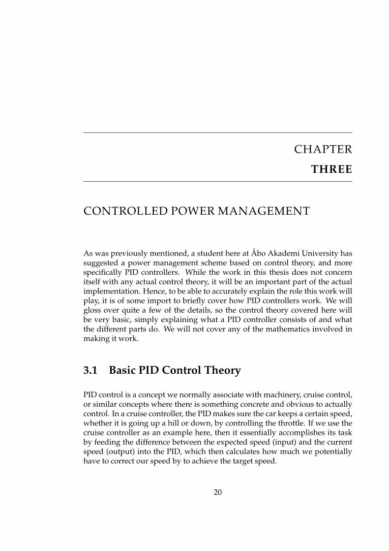
As was previously mentioned, a student here at Åbo Akademi University hassuggested a power management scheme based on control theory, and morespecifically PID controllers. While the work in this thesis does not concernitself with any actual control theory, it will be an important part of the actualimplementation. Hence, to be able to accurately explain the role this work willplay, it is of some import to briefly cover how PID controllers work. We willgloss over quite a few of the details, so the control theory covered here willbe very basic, simply explaining what a PID controller consists of and whatthe different parts do. We will not cover any of the mathematics involved inmaking it work.
3.1 Basic PID Control Theory
PID control is a concept we normally associate with machinery, cruise control,or similar concepts where there is something concrete and obvious to actuallycontrol. In a cruise controller, the PID makes sure the car keeps a certain speed,whether it is going up a hill or down, by controlling the throttle. If we use thecruise controller as an example here, then it essentially accomplishes its taskby feeding the difference between the expected speed (input) and the currentspeed (output) into the PID, which then calculates how much we potentiallyhave to correct our speed by to achieve the target speed.
20

Figure 3.1: A very simple example of a PID controller.
Figure 3.1 shows us a simplified block diagram of the aforementioned PIDcontroller setup. The input block is assumed to contain all sensors andhardware necessary to produce an input value, i.e. the target speed, fromwhich we then subtract the fed back value, i.e. the current speed, to get theerror value. The error value is then sent to the PID. The resulting equationmight look something like:
e = r − y (3.1)
where e (error) is the PID input value, r is the target value, and y is theoutput and feedback value. From the PID block we then get the sum of threecalculations.
• Proportional calculationKpe(t) (3.2)
where Kp is the proportional gain, and e(t) is the error at time t.Increasing the Kp value will result in a larger error value and thereforea more drastic correction. Conversely, if Kp is small, we will see a lessdrastic correction to an error.
• Integral calculation
Ki
∫ t
0
e(τ)dτ (3.3)
where Ki is the integral gain, and e(τ) the error integrated from time 0to now. The integral will contain the sum of all previous instantaneouserrors and will therefore help us reach the target value quicker, providedwe have chosen a proper Ki value. If the value is too large, we willoscillate around the target value, and if it is too small, we will approachthe target value very slowly.
• Derivative calculationKd
d
dte(t) (3.4)
where Kd is the derivative gain, and e(t) will be differentiated withrespect to time. This calculation will help us slow the output’s rate of
21

change. A large Kd means a slower change, where a smaller value meansa quicker change. As opposed to the proportional calculation, which letsthe controller react quicker or slower, the derivative calculation dampensovershoot and oscillation around the target value.
The sum of these three calculations is then fed into the device we wish tocontrol. Using the same example as earlier, this would be a cruise controller.The cruise controller then uses the newly acquired value to adjust the throttleand therefore the current speed, and the resulting speed is again fed back andlets us calculate a new error to use as an input.
3.2 Controlling a Web Cluster using a PID
To paraphrase [19]: a system level controller can make a cluster of low-powerservers power proportional. The controller will use sleep states to switchCPUs on or off in order to continuously match the current workload withthe system’s capacity. It uses methods from control theory to drive the CPUsfrom and into sleep states. Results from system simulation show that thisapproach can achieve a up to 80% reduction in energy consumption comparedto a cluster using only DVFS.
In the previous section we used a cruise controller as an example to explaina PID controller. While applying the same concept to a web cluster’s powermanager may seem different at first, it is actually fairly similar. We use thesame formula - eq. 3.1 - to calculate our input, output and error values, theyjust refer to different things. Here we will use the system’s work load - in termsof number of requests per second - as our target value. System capacity ismeasured in maximum number of requests per second the system can handle,which, when we know the number of CPUs in the system, translates into thenumber of CPUs we need to meet the demand, or target value if you will. Thisis also our feedback value. The difference between the work load and numberof active CPUs is then used to calculate the error value [19].
This scheme will not work if no one takes responsibility for turning CPUs onand off, which is why one core will be kept statically active. The static core willalso be used to handle the low number of requests trickling in when the systemis otherwise almost idle between peak hours. Currently, as the system in ourreference was built around ARM Cortex-A8 CPUs, once a CPU is activated bythe power manager (PM), it will run at the highest possible frequency. Thisis not, from a power consumption point of view, ideal, even though the ARMCPUs are designed to consume very little power [19][20].
22

Also, because the only scheduler currently available is the CFS, which bydesign uses all resources equally, we run into trouble whenever the workloaddrops. While the workload increases the PID will keep turning on CPUs tomeet the demand, so they will all be fully loaded per definition. When thedemand starts dropping off, however, CFS will start spreading tasks out overall the available CPUs. This in turn will mean the PID will be unable to switchthe CPUs off. Therefore, as the PID is unable to influence scheduling, wewill need a scheduler capable of reliably consolidating tasks on as few CPUsas possible, ideally with a negligible impact on performance. It is currentlyunclear as to whether or not CFS, even with _MC or _SMT , is capable of this.We will thus change the behaviour of the CFS to fill CPUs sequentially and itsLB to always keep as many CPUs as possible fully loaded. These changes willthen be compared against the original CFS both with and without its power-saving options turned on. This is how the work in this thesis relates to the PIDControlled Power Manager. We have been looking at ways to schedule tasksin a way that is beneficial both for the energy efficiency and performance.
23

CHAPTER
FOUR
PROPOSED SCHEDULER CHANGES
In Chapter 3 we concluded an ideal scheduler for the PID PM would fill CPUswith tasks sequentially and its LB would ensure that we use as few CPUs aspossible. When we herein say "sequentially" we mean; scheduling tasks ontoone CPU until it has reached its maximum capacity. CFS does not currently dothis - see Chapter 2. Even with its supposed power-saving options turned on,it will first schedule tasks onto all available CPUs and then during LB attemptto consolidate tasks. This is based on an impression gotten from reading theKernel code however, so it will be tested in LinSched. LinSched as a tool iscovered in Chapter 5.1.
In this chapter we will explain the changes made to the CFS’ code as an attemptto improve its power-saving capabilities. The scheduler we get from usingthese changes will henceforth be referred to as the Overlord Guided Scheduler(OGS). The name is a play at the fact that the PID, our Overlord, might decideto turn almost everything off at any time. Since we will only change theselection algorithms we will not have to concern ourselves with any lockingmechanisms, which is quite fortunate since LinSched does not help verifylocking. Still, to be on the safe side we will verify that changing the selectionof RQs does not somehow circumvent the current locking mechanisms will.There was, however, no time to do this during this thesis project and it willthus be recommended as Further Work.
The changes suggested below, disregarding the proposed LB changes, havebeen spliced into the original CFS code at the appropriate places. The OGScode has been put behind #ifdef declarations, and will thus only be included
24

and used when expressly chosen at the Kernel build stage. If we do not selectOGS, then the CFS scheduler is used in its original state. Building a Kernelwith the tweaked code and using only the default build options will resultin the Kernel using CFS. We have attempted to splice the proposed schedulerchanges into the existing scheduler instead of writing it from scratch becauseof the time constraints imposed on this thesis project. Had we decided towrite one from scratch, we would, for instance, have had to understand andimplement locking, which in itself would have easily used more than theamount of time we had available.
4.1 Runqueue Selection
Every new task has to be scheduled on a RQ on some CPU. For CFS this isalways the idlest RQ, as was explained in Chapter 2.1.2. To make good use ofthe PID PM we want to always schedule tasks on the busiest non-overloadedRQ.
Using LinSched and a number of well placed text prints, as well as bylooking at the Kernel code we identified select_task_rq() as the functionmaking all the important decisions regarding RQ selection. This function thenmakes a task class-specific call to another function which makes the ultimateselection and returns it. We have not bothered with RT tasks due to the timeconstraints of this project, and thus the selection function we are interested inis select_task_rq_fair(). This function is called whenever a RQ is to be selectedfor a task falling under the influence of the CFS and we then proceed to makea RQ selection as was specified in Chapter 2.1.2. Looking at this function wecan come to the conclusion that in order to change the RQ returned by thisfunction, we need to change what find_idlest_group() and find_idlest_cpu()decide to return.
4.1.1 find_idlest_group() vs find_busy_group()
The current implementation of this function will, as the name implies, returnthe idlest SG from a given SD based on SGs’ average weighted load. The codebelow is copied from find_idlest_group() in the 2.6.35 version of the LinuxKernel. It is the part of that function upon which all decisions are based. Thelines have been numbered after copying to make referencing it easier.
1 /* Tally up the load of all CPUs in the group */2 avg_load = 0;
25

34 for_each_cpu(i, sched_group_cpus(group)) {5 /* Bias balancing toward cpus of our domain */6 if (local_group)7 load = source_load(i, load_idx);8 else9 load = target_load(i, load_idx);1011 avg_load += load;12 }1314 /* Adjust by relative CPU power of the group */15 avg_load = (avg_load * SCHED_LOAD_SCALE) / group->cpu_power;1617 if (local_group) {18 this_load = avg_load;19 this = group;20 } else if (avg_load < min_load) {21 min_load = avg_load;22 idlest = group;23 }
It is easy to see that the for-loop starting on Line4 iterates through all membersof the SG and tallies the total load. What is unclear is how the perceived loadchanges depending on whether the group is local or not - Lines6− 9. Based onthe code comments we do know it is supposed to bias the selection towardsa local group. Looking at the definitions of source_load() and target_load() insched.c we can see that the bias lies in the size of the weighted_cpuload() thatis added to avg_load on Line11. This again takes us back to the problem ofload weights and their lacking documentation. Sorting out the exact way theload weights work and are assigned was, as we mentioned earlier, deemedto exceed the scope of this project. Although the general impression is thatassigning weights to tasks may not result in a, for our purposes, ideal taskdistribution. This will affect our ability to detect the current load as well, whatwith the current upper limit also being based on load weights. The PID willneed a feedback value telling us whether or not we are likely to need to turnon more CPUs, therefore we have another problem.
One solution to these problems would be to make these decisions based onhow idle a CPU has been since we last scheduled a task on it. This isessentially already done by the Governors - covered in Chapter 2.2 - as theylook at how idle a CPU is and adjusts the CPU’s frequency accordingly. Asall the functionality is already in place, it would then be a short step to use
26

the same information when making decisions regarding RQ selection. Forthe Governors to work, there needs to be a structure storing all the differentcontributions to the CPUs utilisation. This structure is already defined ininclude_linux_kernel_stat.h, so there is no need to define another. The updatefunctions for the CPUs’ busy times are also already in place. Using theinformation gathered on behalf of the Governors to make our RQ selectionsis then a trivial matter.
25 static struct sched_group *26 find_busy_group(struct sched_domain *sd, struct
task_struct *p, int this_cpu,cputime64_t time_now)
27 {28 struct sched_group *busy_group = NULL,
*group = sd->groups;29 // To keep track of the most loaded group30 cputime64_t min_idle = time_now;31 cputime64_t idle_time; // Time spent idle32 cputime64_t SAFETY_MARGIN = 100000; //Arbitrary number3334 do {35 int i;3637 /* Skip groups with no CPUs allowed */38 if (!cpumask_intersects(sched_group_cpus(group),
&p->cpus_allowed))39 continue;4041 /* Reset idle_time and safety for each group */42 idle_time = 0;43 safety = 0;4445 for_each_cpu(i, sched_group_cpus(group))46 {47 idle_time = cputime64_add(idle_time,
what_is_idle_time(i, time_now));48 safety += SAFETY_MARGIN;49 }5051 if( (idle_time < min_idle) && (idle_time > safety) )52 {53 min_idle = idle_time;54 busy_group = group;
27
55 }5657 }while(group = group->next, group != sd->groups);5859 if(!busy_group)60 {61 return NULL;62 }6364 return busy_group;65 }
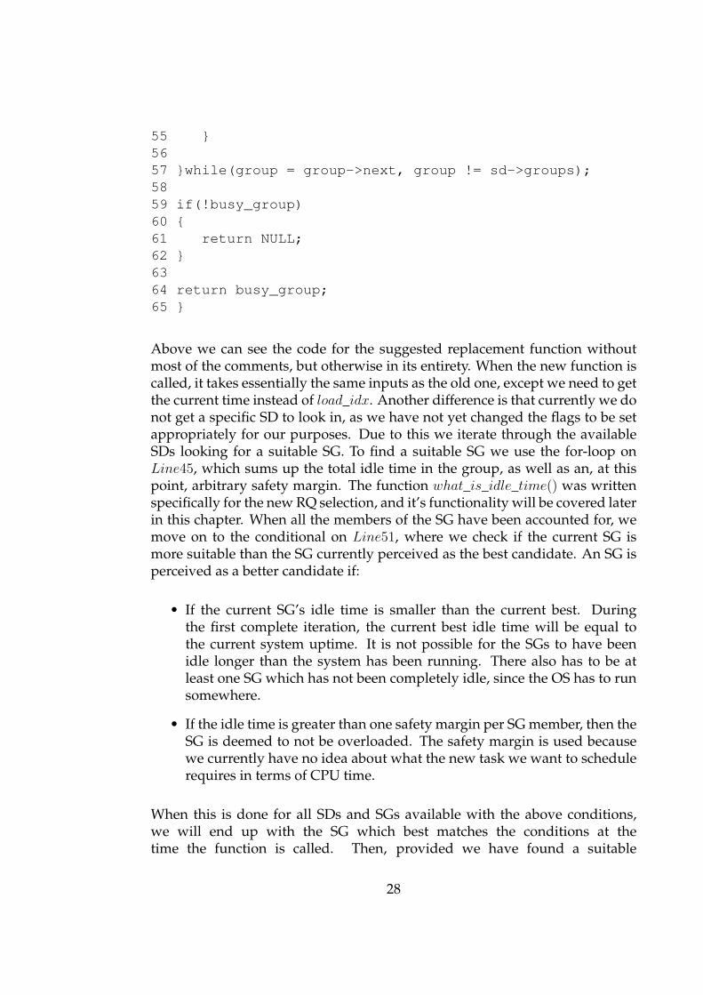
Above we can see the code for the suggested replacement function withoutmost of the comments, but otherwise in its entirety. When the new function iscalled, it takes essentially the same inputs as the old one, except we need to getthe current time instead of load_idx. Another difference is that currently we donot get a specific SD to look in, as we have not yet changed the flags to be setappropriately for our purposes. Due to this we iterate through the availableSDs looking for a suitable SG. To find a suitable SG we use the for-loop onLine45, which sums up the total idle time in the group, as well as an, at thispoint, arbitrary safety margin. The function what_is_idle_time() was writtenspecifically for the new RQ selection, and it’s functionality will be covered laterin this chapter. When all the members of the SG have been accounted for, wemove on to the conditional on Line51, where we check if the current SG ismore suitable than the SG currently perceived as the best candidate. An SG isperceived as a better candidate if:
• If the current SG’s idle time is smaller than the current best. Duringthe first complete iteration, the current best idle time will be equal tothe current system uptime. It is not possible for the SGs to have beenidle longer than the system has been running. There also has to be atleast one SG which has not been completely idle, since the OS has to runsomewhere.
• If the idle time is greater than one safety margin per SG member, then theSG is deemed to not be overloaded. The safety margin is used becausewe currently have no idea about what the new task we want to schedulerequires in terms of CPU time.
When this is done for all SDs and SGs available with the above conditions,we will end up with the SG which best matches the conditions at thetime the function is called. Then, provided we have found a suitable
28

candidate SG, we return it to select_task_rq_fair() and used as an input infind_busy_sched_cpu().
4.1.2 find_idlest_cpu() vs find_busy_sched_cpu()
The current implementation of this function suffers from the same prob-lems as find_idlest_group(). As can be seen on Line72 below, it isbased around weighted_cpuload(). Using the SG reported as the idlestby find_idlest_group(), we iterate through the group members looking forthe CPU with the smallest load. The found CPU is then returned toselect_task_rq_fair() and will be selected as the target RQ for the new task.This, again, is not in line with our aims. We would like to select the RQ withthe highest load available, while not overloading its CPU.
70 /* Traverse only the allowed CPUs */71 for_each_cpu_and(i, sched_group_cpus(group),&p->cpus_allowed) {72 load = weighted_cpuload(i);7374 if (load < min_load || (load == min_load && i == this_cpu)) {75 min_load = load;76 idlest = i;77 }78 }79 return idlest;
Below we have the suggested replacement function, which would worktogether with find_busy_group() in finding a suitable RQ to schedule on, inits entirety. Again without most of the comments.
The replacement function here is quite similar to the original in that it does thesame kind of iteration - starting on Line94 - through all the CPUs in the group.The main difference here is that, again, we look at how idle the CPU has been,instead of its weighted_cpuload(). Then, on Line99 we get the RQ struct for thecurrent CPU, which contains information about the number of tasks runningon this CPU. We do this because we will, on Line104, calculate how muchexecution time the currently running tasks require on average. This averagewill then be used as an estimate of how much execution time the new task islikely to require. Estimating task requirements using an average is not an idealsolution, as it is quite likely to over- or underestimate the amount of time thenew task will require. Although, since we currently have no way of knowing
29

anything about new tasks, this solution will at least give us an estimate of howmuch busier another task might make the CPU.
85 static int86 find_busy_sched_cpu(struct sched_group *group,
struct task_struct *p, int this_cpu,cputime64_t time_now)
87 {88 int busy_sched = -1;89 int i;90 cputime64_t idle_time = 0;91 cputime64_t avg_busy_time_per_task;92 cputime64_t min_idle = time_now;9394 for_each_cpu(i, sched_group_cpus(group))95 {96 /* Get the time cpu(i) has spent idle */97 idle_time = what_is_idle_time(i, time_now);9899 struct rq *arr_qu = cpu_rq(i);100101 if (arr_qu->nr_running < 1)102 avg_busy_time_per_task = 0;103 else104 avg_busy_time_per_task = cputime64_sub(time_now,
idle_time)/(arr_qu->nr_running);
105106 if ( (idle_time < min_idle) && (idle_time >
(SAFETY_MARGIN+avg_busy_time_per_task)) )107 {108 min_idle = idle_time; //refresh the reference value109 busy_sched = i; //record which cpu this is110 }111 }112113 return busy_sched;114 }
Before calculating said average - on Line102 - we make sure we have at leastone task running before calculating the average. If no tasks are running onthe CPU, then the average busy time per task is set to naught. Otherwise we
30

calculate the average normally. This is to avoid a potential division by zero.Once we have an average, we compare the idle time against the current best.We conclude we have found a new target CPU if:
• The current idle time is lower than the current best. The initial best valueis, again, the current system uptime.
• The current idle time is higher than the sum of the safety margin and theaverage busy time per task. This is again a safety mechanism, which isused due to the uncertainty around the new task’s requirements.
Once we have found a suitable target CPU, we return it to select_task_rq_fair()and schedule the new task on it. If this function returns a null value, thenwe obviously need an alternative target CPU. This goes for the default CFSas well. Fortunately select_task_rq() - i.e. the function calling the task-specificRQ selection function from sched.c - already has a function taking care of this inselect_fallback_rq(). This function has currently been left as is. Suffice to sayit makes sure we find somewhere to schedule our task, even if our selectionmethod found all CPUs to be unsuitable. At a later stage this function shouldalso be looked at in order to find out whether or not it has to be changed.
The accuracy of our selection procedure will have to be evaluated, as it isquite heavily dependent on the average busy time calculation. If a CPU hasa few tasks taking up a large portion of the available execution time, thenthe consequently high average may cause us to choose another CPU, even ifthe aforementioned CPU would be capable of handling a few low load taskswithout being overloaded. It is possible that this problem is best solved duringLB, and a possible, although not yet investigated solution will be mentionedin Section 4.2.
4.1.3 what_is_idle_time()
This function was put in sched_fair.c for the express purpose of getting andreporting a CPU’s idle time to OGS’ RQ selection functions. It is essentiallyidentical to the equivalent function - get_cpu_idle_time_jiffy() - used by, e.g.,the Ondemand Governor. The only differences being that the current systemuptime here, time_now, is not a pointer and that we, on Line132, make sure wehave no negative idle time values. It should not be possible to have a busy timethat is longer than the system uptime, but due to some of the workaroundsused in LinSched, detailed in Section 5.1.3, it did happen occasionally. Thecondition has been left in as a safety mechanism.
31

What this function then needs to work properly is a CPU, and the currentsystem uptime. Which CPU we’ll be looking at is normally given by anunsigned int, which is basically the CPU’s ID number as far as the Kernel isconcerned. The current system uptime is here stored in the variable time_now.Its value is gotten from a check in select_task_rq_fair() and given as an inputto the find_busy_∗ functions, which pass it on to this function. We are currentlydoing it this way as it keeps both the number of time checks down, andtime_now constant for the duration of the RQ selection process. There is asmall chance that changing time_now mid-selection will warp the result, henceits being constant while we are looking for a RQ.
Lines127 − 130 are the ones where we actually add the busy times. Judgingfrom the structure in kernel_stat.h, the Kernel distinguishes between fivedifferent types of business, and these types are stored as elements in saidstructure. The total business is then the sum of the five business types, withthe idle time - idling - being the difference between this sum - i.e. busy_time -and time_now. The difference is then returned to the calling function.
120 static inline cputime64_twhat_is_idle_time(unsigned int cpu,
cputime64_t time_now) {121122 /* Variables for tallying idle time */123 cputime64_t busy_time; // Time spent busy124 cputime64_t idling; // Temp variable125126 /* Tallying the idle time */127 busy_time = cputime64_add(kstat_cpu(cpu).cpustat.user,
kstat_cpu(cpu).cpustat.system);128 busy_time = cputime64_add(busy_time,
kstat_cpu(cpu).cpustat.softirq);129 busy_time = cputime64_add(busy_time,
kstat_cpu(cpu).cpustat.steal);130 busy_time = cputime64_add(busy_time,
kstat_cpu(cpu).cpustat.nice);131132 if (unlikely(busy_time > time_now))133 idling = 0;134 else135 idling = cputime64_sub(time_now, busy_time);136137138 return jiffies_to_usecs(idling);
32

139 }
It is possible we will not even need this function in a full Kernel adaptation,however the experimentation herein was done using LinSched, which onlyuses the parts necessary to emulate the normal scheduling subsystem, and nofunctionality from the CPUfreq subsystem was therefore available.
To reiterate then; the changes mentioned above, called OGS, will move usaway from selecting the idlest RQ and to selecting the busiest RQ with someremaining capacity. The capacity is determined by summing up the differenttypes of business stored in the cpu_usage_stat struct in kernel_stat.h. Wecurrently go through all the SDs to find the SG with the most suitable idletime, and then move on to find the CPU with the most suitable idle time in thepreviously detected SG. It is our feeling that making RQ selection decisionsbased on how idle a CPU has been may lead to a load distribution that iscloser to the, for our purposes, ideal distribution compared to CFS’ schemewith weighted tasks. Said ideal distribution would have the tasks scheduledon as few CPUs as possible. It is also a lot easier to detect when a CPU isabout to become fully loaded when using OGS, which is extremely importantin order for the PID controller to be able to work properly, as we can simplylook at how close to naught the idle time is. Neither do we need to store anyinformation relating specifically to the capacity of the available CPUs, since,again, the information is already available in the idle time and its approachingnaught. We therefore only need the current system uptime, the number oftasks belonging to the RQ, and how busy the CPU has been in order to makeour RQ selection. All of these are already available in the kernel. The systemuptime is stored in a variable called jiffies, the number of tasks in a RQ isan externally visible scheduling statistic, while the Governors keep track of aCPU’s busy time.
Figure 4.1 above illustrates how CFS and the weighted CPU load is assumed toaffect the perceived business of a CPU compared to OGS and idle time. EachL-shaped block represents one task and its execution time requirements, whilethe space it takes up in the figure is equivalent to how the scheduler perceivesit. Both schedulers have one CPU at their disposal in this illustration. Ourassumption then is that the load weights may cause the CFS RQ selection toperceive each task as requiring an execution time equivalent to a 2-by-3 blockinstead of its actual requirement. Due to this, it might see a CPU as being fullyloaded after 16 tasks have been scheduled on the CPU in question. The OGSon the other hand, is capable of detecting how much time the scheduled taskshave actually been using and is therefore able to schedule tasks in such a waythat we use our CPUs more efficiently in terms of execution time. Again; this is
33

Figure 4.1: Illustration of how the weighted CPU load is assumed to affectperceived business
an assumption about the CFS and our aim for the OGS, and we will thereforeattempt to validate said assumption and aim empirically.
The changes detailed in this section (4.1) only affect the RQ selection process.The function charged with finding a RQ for new tasks is the only one we havechanged. Therefore, as CFS should work quite well for our purposes whenusing the OGS RQ selection, we use the original CFS code for, e.g., locking,and actually giving tasks CPU time.
4.2 Load Balancing
As was explained in Section 2.1.3, the CFS LB will by default attempt to achievean even task distribution. This means the LB will always pull tasks from thebusiest to this RQ. While CFS does have the SCHED_MC and SCHED_SMToptions for pulling tasks from almost idle RQs, they only seem to work incases where we have a as-good-as idle RQ, and pulling tasks from it would notupset the otherwise even task distribution, whereas we would like to minimisethe number of CPUs in use by keeping the load as high as possible withoutoverloading. We will attempt to show this in Chapter 6. Although we do havea relatively clear idea of what we would like to implement, we currently onlyhave a superficial plan for affecting this change. The herein proposed changeshave therefore not been tested.
34

The CFS LB works according to our needs as far as Step 5, by the reckoningused in Chapter 2.1.3. When we get as far as Step 5, we start looking forsource and target RQs. We will refer to the RQ from which we pull a taskas the source RQ, and to the RQ performing the pull as the target RQ here. Atthis stage CFS finds the busiest queue - find_busiest_queue() - in the busiestgroup - find_busiest_group(). When finding the group, CFS uses a struct calledsd_lb_stats. This struct is updated every time the group-finding function iscalled, and contains information relevant to LB at this level. The elements areused at various points by different functions to achieve a balanced load.
4.2.1 find_busiest_group()
The elements used by find_busiest_group() to decide if we are imbalanced are:
• sds.this_load (struct sd_lb_stats sds) - Contains the perceived load of thewe are a member of.
• sds.busiest - The currently busiest group
• sds.busiest_nr_running - The number of tasks running in the busiestgroup
• sds.max_load - The highest group load in this SD
• sds.avg_load - The average load in this SD
• balance - An integer value, used as a boolean, which indicates whetherthis is the appropriate CPU to perform LB at this SD level or not.
We previously - in Chapter 2.1.3 - mentioned that we check a number of caseswhich tell us if there is no imbalance from this CPU’s point of view if. Thesecases are:
• #1 This CPU is not the appropriate CPU to perform LB at this level. Wecheck the value in balance and if it is 0 this CPU is not appropriate andwe jump to ret, otherwise we move on.
• #2 There is no busy sibling group to pull from. Here we look at the busiestand busiest_nr_running elements in sds. If we either have no busiestgroup, or if there are no tasks running, i.e. busiest_nr_running == 0, wejump to out_balanced. In all other cases we move on.
35

• #3 This group is the busiest group. See if sds.this_load >= sds.max_load,which if true means that this group is the busiest group. We want to pullfrom the busiest group, so we jump to out_balanced.
• #4 This group is more busy than the average business in this SD. Tobe able to do this check then, we have to actually calculate an averageload. This is done just before the actual if statement. If sds.this_load >=sds.avg_load, then we do not want to pull tasks to this group, as it wouldnot help us equalise the load.
• #5 The imbalance is within the specified limit. The check we do hereis 100 ∗ sds.max_load <= sd− > imbalance_pct ∗ sds.this_load. Thevalue of imbalance_pct will depend on what SD we are currently lookingat, but the idea is that its value will tell us how much larger max_loadcan be before we see it as being imbalanced. If the imbalance turnsout to be withing the specified limits, we jump to out_balanced. Asan arbitrary example, let’s say max_load = 75, this_load = 55, andimbalance_pct = 125. Using the formula above we would then get7500 <= 6875, which tells us the imbalance is unacceptable. Although,were this_load to increase by 5 units, we would, using the same formula,get 7500 <= 7500, which is within the limits and prompts a jump.
• ret - A point in this function we jump to from #1 when the CPU turns outto be inappropriate. Jumping here will return us to load_balance() with anull group, and with imbalance = 0 - the value of imbalance will later letus know how much load to move in order to equalise the distribution.
• out_balanced - A point in the function we jump to if one of the checks #2-5tells us there was no obvious imbalance. check_power_save_busiest() iscalled from here to see if we have opted for power-saving and whetheror not it is possible to perform such a balancing. Whatever valuecheck_power_save_busiest() returns is then returned to load_balance().
If we clear all these checks, then we will calculate how imbalanced we areusing calculate_imbalance(). The value returned from this function is theamount of weighted load we have to move to equalise the distribution fromthe point of view of this_cpu. We will cover this function, as well as how wewould like to change it, in Subsection 4.2.3 later in this chapter.
As was the case with RQ selection, CFS works counter to our purposes. Now,again, we did not manage to implement LB for OGS within the timeframe ofthis thesis, so the LB changes proposed herein have not been tested and areonly a draft design. We have yet to identify all scenarios where an imbalancedoes not exist from the point of view of this_cpu. One scenario we will most
36

certainly need to check is if this_cpu is the idlest one. If it turns out to bethe idlest, then we want to pull tasks from it and not the other way around.Another scenario would be that this_cpu has no idle time to spare, or itsexcess idle time is smaller than the average busy time per task of idlest. Otherscenarios are are quite likely to exist, but have yet to be identified.
It is our feeling at this point that an equivalent of the check_power_save_busiest()is not needed, since we are attempting to save power by default when usingOGS. A possible substitute for this function could then be a check to see ifone of the busier RQs are overloaded, and whether or not this_cpu couldalleviate the problem. However, this is currently not possible, as we havenot implemented a way of detecting overloads. We can easily detect whenthe idle time is approaching naught, but if the busy time were to exceed theavailable exceution time - exceeding the execution time should here be seenas a problem akin to RTS, where all tasks do not fit in a certain period, andthus we start missing deadlines - as the idle time can never be negative. Thiscould potentially be solved by borrowing from RTS theory. Each task wouldupon creation be given a soft deadline, or an acceptable waiting time if youwill. Once tasks start to occasionally miss these deadlines we can assumethat the RQ is on the verge of becoming overloaded. Once they reliably misstheir deadlines, the RQ is definitely overloaded. This solution is, again, only ahypothesis and has neither been implemented nor tested.
4.2.2 find_busiest_queue()
When looking for the busiest queue we do not need to use an SG structin the same way find_busiest_group() used an SD struct. The searchhas now been refined sufficiently for it to be a lot more efficient to lookdirectly at the RQs of all the CPUs in the chosen group. Using the loopfor(i, sched_group_cpus(group)), Line 1 below, we make sure that we iterateover all the SG members. The unsigned long power will contain what issupposed to be a measurement of the capacity of the current CPU, and theunsigned long capacity is then the measured capacity scaled by a constant;SCHED_LOAD_SCALE. The unsigned long wl will contain the detectedworkload for the CPU we are currently looking at, which we get using a callto weighted_cpuload(). We also get the RQ struct for the current CPU. The RQthat is returned after the last iteration will be the one with the highest wl value- wl is scaled by CPU power, on Line 12, before being compared against theother loads. The if statement on Line 13 then compares the current CPU’s loadagainst the currently highest load, and stores the new values if they turn outto be higher.
37

1 for_each_cpu(i, sched_group_cpus(group)) {2 unsigned long power = power_of(i);3 unsigned long capacity = DIV_ROUND_CLOSEST(power,
SCHED_LOAD_SCALE);4 unsigned long wl;56 if (!cpumask_test_cpu(i, cpus))7 continue;
8 rq = cpu_rq(i);9 wl = weighted_cpuload(i);
/** When comparing with imbalance, use weighted_cpuload()
* which is not scaled with the cpu power.
*/10 if (capacity && rq->nr_running == 1 && wl > imbalance)11 continue;
/** For the load comparisons with the other cpu’s, consider
* the weighted_cpuload() scaled with the cpu power, so that
* the load can be moved away from the cpu that is potentially
* running at a lower capacity.
*/12 wl = (wl * SCHED_LOAD_SCALE) / power;
13 if (wl > max_load) {14 max_load = wl;15 busiest = rq;
}}
In order for the OGS LB to work as planned, we would like to find the idlestqueue with at least one task running. One possible solution would be along thelines of the code below. Here we would iterate through the SG members usingthe same for-loop as with CFS. Now though we will start out by declaring anunsigned long it, short for idle time, which we will use to find the largest idletime of any CPU and RQ with at least one task running. The if statementon Line 26 will force us to move on to the next iteration if the current RQhas no tasks running, as per the idlest queue with at least one task runningrequirement, and the if statement on Line 28 will store the RQ with the largestidle time. The RQ will still be stored in busiest, which may sound like a curious
38

choice for a variable’s name, but since OGS has essentially been spliced into theoriginal CFS code, we have tried to change as little as possible to ensure bothschedulers can be compiled interchangeably from the same code.
20 for_each_cpu(i, sched_group_cpus(group)) {21 unsigned long it;
22 if (!cpumask_test_cpu(i, cpus))23 continue;
24 rq = cpu_rq(i);25 it = what_is_idle_time(i, time_now);
/* *** If rq is empty, then skip it.
* There should never be a case where ALL rqs are empty,
* since LB is invoked AFTER we’ve got a few tasks running
** nr_running < 1, since we don’t want to pull from an empty RQ
*/26 if (rq->nr_running < 1 )27 continue;
/** For the load comparisons with the other cpu’s,
*/28 if (it > max_idle) {29 max_load = it;30 busiest = rq;}}
Again; these changes have not been tested yet, but, provided the group-findingfunction works as intended, they should work more or less as-is. The testingof these functions subsequently has to fall under Future Work.
Another couple of things that will have to be worked on in the future arethe functions update_sd_lb_stats() and update_sg_lb_stats(). These functionsupdate their respective LB stats structures, and currently only do it for thebenefit of CFS. If the OGS LB is to work properly, we need to either tweakthese functions or write new ones which will update an SD- and an SG-relatedstruct with data relevant for OGS LB.
39

4.2.3 calculate_imbalance()
To paraphrase the comments in the code: calculate_imbalance calculates theamount of imbalance within the groups of a given SD during LB. As inputsit uses sds, which was earlier defined as SD statistics relevant to LB, this_cpu,which is the CPU for which LB is being performed - and in the case of CFSLB, the CPU to which tasks will be pulled - and then output the results tothe variable imbalance. All of the code excerpts here are from the functioncalculate_imbalance() in sched_fair.c.
sds->busiest_load_per_task /= sds->busiest_nr_running;if (sds->group_imb) {sds->busiest_load_per_task =min(sds->busiest_load_per_task, sds->avg_load);}
Before CFS calculates the actual imbalance we check if an SG has re-ported an internal imbalance. An SG considers itself imbalanced if thedifference between its max_load and min_load is more than twice theavg_load_per_task in the group. This is checked and potentially updatedevery time update_sg_lb_stats() is called, which happens as an extensionof the initialisation calls at the start of find_busiest_group(). If an SGhas reported being internally imbalanced, CFS will use the smaller valueof busiest_load_per_task and avg_load as its recorded busiest_load_per_taskvalue, as can be seen from the code excerpt above.
According to the comments in the Kernel code, there are some cases whenusing SMP Nice balancing where max_load is smaller than avg_load. Judgingfrom the comment, SMP Nice will skip groups at or below its capacitywhile calculating max_load [3]. Whenever this happens, calculate_imbalancewill return an imbalance of naught and call fix_small_imbalance() beforereturning to find_busiest_group().
Then, if we did not find one group to be internally imbalanced, CFS willtake a look at the busiest SG to see how much more than its capacityit is currently executing. This check is performed by the code excerptbelow, where load_above_capacity will be scaled according to the constantSCHED_LOAD_SCALE and the SG’s scaled capacity. The resulting valueshould be something along the lines of a weighted percentage above capacity.
if (!sds->group_imb) {/*
40

* Don’t want to pull so many tasks that a group would go idle.
*/load_above_capacity = (sds->busiest_nr_running -sds->busiest_group_capacity);
load_above_capacity *= (SCHED_LOAD_SCALE * SCHED_LOAD_SCALE);
load_above_capacity /= sds->busiest->cpu_power;}
Next, CFS will look for the minimum possible imbalance to correct. Judgingfrom the comment left at this stage of the code, the reasoning behind this isthat if all SGs take on a small amount of the load perceived as imbalance, thenthe distribution will eventually be equalised. By this reckoning then, CFS willreport the smallest detected imbalance, as per Line 1 in the excerpt below. OnLine 2 CFS then checks how much of the imbalanced load this_cpu could pull.If the scaled difference between the average load and this_load is greater thanthe amount of detected imbalance, then the function will report that all of itcan be pulled.
/** We’re trying to get all the cpus to the average_load,
* so we don’t want to push ourselves above the average load,
* nor do we wish to reduce the max loaded cpu below the
* average load. At the same time, * we also don’t want to
* reduce the group load below the group capacity (so that we
* can implement power-savings policies etc). Thus we look
* for the minimum possible imbalance.
* Be careful of negative numbers as they’ll appear as very
* large values with unsigned longs.
*/1 max_pull = min(sds->max_load - sds->avg_load,load_above_capacity);
/* How much load to actually move to equalise the imbalance */2 *imbalance = min(max_pull * sds->busiest->cpu_power,(sds->avg_load - sds->this_load) *sds->this->cpu_power)/ SCHED_LOAD_SCALE;
On the off chance the detected imbalance is negligible, there is no guaranteeanything will be moved so before returning, CFS will do one last check to seewhether or not imbalance is larger than the average load per task on busiest
41
- i.e. busiest_load_per_task - which is the future pull target. If this turnsout to be the case, then CFS will call fix_small_imbalance() to ensure the LBtakes a closer look at load distribution, even though the detected imbalanceis negligible. Although, there is no guarantee fix_small_imbalance() willactually move anything.
In our case, i.e. the OGS imbalance calculation, we would like to know howmuch below capacity the CPUs in the busiest groups are. As we have saidbefore, the purpose of OGS is to use as few CPUs as possible by filling them tocapacity. An imbalance in our case then would be when this_cpu has an idletime larger than the average busy time per task and is not ranked as idlest.The planned LB procedure would then look at the average load per task inthe idlest RQ, with at least one task running, compare this value against theaverage load per task in this_cpu, and pull as many tasks as this comparisonsays is possible. The OGS imbalance calculation would then be somethingalong the lines of:
imbalance =this_cpu.idle_time
idlest.avg_busy_time_per_task(4.1)
where imbalance - this value will have to be rounded down and comparedagainst the number of tasks running on idlest ensure we do not attemptto pull more tasks than are available - is the number of tasks we wantto pull, this_cpu.idle_time is the current excess capacity on this_cpu, andidlest.avg_busy_time_per_task is the average contribution per task to thebusiness of idlest. Calculating the imbalance in this fashion should take careof safeguarding against pulling too many tasks to this_cpu while still pullingas many tasks as possible from idlest. Of course, this is still only, as has beenmentioned several times with regards to OGS LB, a hypothesis. A heads upof how we would like to change it if you will, so actually implementing andtesting this will fall under future work
4.2.4 move_tasks()
After we have found both a group and a RQ it is time to move tasks andattempt to equalise the distribution. As its name implies, this is done using thefunction move_tasks(). The call returns the amount of load that was actuallymoved, which if greater than naught indicates the LB was successful.
The moving procedure consists of calling load_balance_fair() repeatedly whilethe moved load is smaller than the reported imbalance. This function does notseem to need any changes. If we have managed to change the LB procedure
42

successfully, then all the variables necessary to move tasks according to ourwishes should have been included in the function call. Then, from this functionon it seems we need not change anything.
43
CHAPTER
FIVE
TOOLS, EXPERIMENTATION AND TESTING
5.1 Linsched
Scheduling is one of the most complex aspects of the Linux kernel. Developingschedulers or changing policies and thereafter verifying their behaviour canbe very challenging without the necessary experience. Fortunately there havebeen some recent advances in this area with the development of LinSched.LinSched is a user-space Linux scheduler simulator which hosts the prototypescheduler in user-space and models it against arbitrary hardware targets inorder to validate said prototype across a wide spectrum of topologies [15].
Traditionally new schedulers and policies would have had to be implementeddirectly in the kernel, which, due to the depth at which the scheduler resides,made measuring performance and debugging difficult. Adding traces couldpotentially change the scheduler’s behaviour and possibly even hide defectsand inefficiencies. Not to mention that repeating the procedure for everytopology one wishes to use is too time-consuming to be practical. LinSchedcircumvents these difficulties by migrating the scheduler sub-system into user-space and adds a thin emulation of the components necessary for the schedulerto be able to execute outside of the kernel. In order to be able to provide thestimuli necessary for workload validation it also builds a set of applicationprogramming interfaces (APIs) around it. This also allows us to gather enoughrelevant data to understand and measure the scheduler’s behaviour. Anotherupside to this approach is that a misbehaving scheduler potentially causing a
44

Figure 5.1: LinSched Scheduler Simulator Architecture [15]
crash will not bring down the entire machine [15].
The above figure is an illustration of LinSched’s architecture. Starting fromthe bottom we have the host operating system (HOS), which in our case is theLinux kernel. On top of the HOS and on the lowest level in user-space, we havethe Environment Module which provides the abstraction of the kernel. Nextin an upward order we have the simulation engine, which extends an APIfor use in configuring the environment and performing the simulation. ThisAPI provides an initialisation function that also defines the processor topologyand functions for creating tasks, callbacks and a run function to perform thesimulation for a certain number of ticks. Above the simulation engine we findthe script environment wherein the actual simulation code resides. [15]
5.1.1 LinSched Tasks
A task in LinSched can be one of four types; normal, batch, first in-first out(FIFO) or round robin (RR). Their sleep and run times can also be specified, butwill be static, insofar the scheduler actually serves them, once the simulation isrunning. They are also currently persistent in the sense that they will want torun periodically for the duration of the simulation. It is also possible to definea subset of CPUs on which a task is allowed to run. When using CFS this doesnot affect the RQ selection in any way other than forcing the tasks to run on the
45

CPU, or CPUs, to which they are bound. When using OGS on the other hand,we should see the CPU, or CPUs, to which tasks have been bound being filledup first. CPU binding will thus be used to ensure that OGS selects the correctRQ to fill up first [15].
5.1.2 Simulator Limitations
The task persistence is, for our purposes, a quite severe limitation as it willaffect the LB and making it essentially impossible to tell if the LB worksas intended. It is possible to ensure we get, for the scheduling policy andtopology in use, an ideal task distribution, but since there is no way ofremoving tasks from the simulation once they have been created, we have noway of knowing how the LB will behave when the scheduling circumstanceschange. This has to be taken into consideration when interpreting the resultsgathered from LinSched.
Another limitation in LinSched is caused by the emulated kernel not being afull version. Due to this we are missing some functionality needed for OGS towork properly. Since OGS bases its scheduling decisions on the busy and idletime of individual CPUs, there is a need for timing updates in order to keeptrack of the amount of time each of the CPUs have been busy. These timingsneed to be stored in a CPU-specific structure as well. There is also a need for avariable keeping track of the amount of time the simulation has been runningin order to be able to calculate for how long a CPU has been busy. None ofthese features are included in LinSched, which necessitates a workaround.
5.1.3 Workarounds
The time-keeping issue was solved by using the jiffies value from the HOSand adjusting that using a modulo operation where the divisor equals thesimulation time in milliseconds. This is not a perfect solution, as there is noguarantee the time will start from naught nor that it will not overflow mid-simulation. It is however a solution that is good enough to make sure OGSworks as intended.
To save the CPU’s busy times the kernel normally uses a structure defined in aheader file kernel_stat.h. Normally there would be one structure defined perCPU, but this is not the case in LinSched. Most likely because the schedulercode is only compiled once and then just in a generic sense and not based onthe topologies we intend to simulate. To get around this we have opted touse an identical structure in a separate file called faked_kstat.h and define an
46
array of 100 samples of the structure therein. As the largest number of CPUscurrently simulated is 24 we thus have more than enough for our purposes. Itwas decided that 100 structures was a suitable number in case there was evera need to simulate a larger system and if need be this number can be changedto whatever size we wish simply by changing the value of a constant definedat the top of the file containing the relevant code; sched_fair.c.
Linux’s default timing update functions are not included either, essentiallymeaning that there is no busy time accounting in LinSched. This is crucialfor OGS and the scheduling decisions it makes. To solve this we have addedfunctions which fake the aforementioned busy time accounting. They are quitesimple and just add an arbitrary time to each of the elements in the time-keeping structure. As we want the updates to resemble an actual systemthe update function calls have been added to the functions in sched.c whichare called when a task is created - wake_up_new_task - and when a task iswoken up to be put on a CPU - try_to_wake_up. While this solution means therecorded runtime does not necessarily correspond to the actual one defined inthe LinSched simulation script, it does mean that we can adjust the amountof busy time a task contributes and since OGS bases its decisions on thesefigures it will still let us verify and validate the behaviour of the RQ selectionalgorithm.
5.2 Simulated Workloads
As the purpose of OGS is to ensure a CPU’s time is used as efficiently aspossible, we want to test various different loads where the CFS displays aless than ideal time usage. In order to get a more complete picture of howthe two schedulers compare, we will also run tests with workloads where theCFS performs well by definition.The different cases will be outlined here andthe specific parameters used will be covered in Chapter 6 where the acquiredresults are analysed.
One case for which the CFS’ performance, for our purposes, is less than ideal iswhen there are a large number of tasks that require a low amount of run time.Using the default settings for CFS these tasks will be spread out evenly overall available CPU RQs regardless of how much processor time they actuallyneed. Using all CPU’s in a case when all tasks could be run without, orwith a negligible, overhead will dissipate more energy than is necessary. TheCONFIG_SCHED_MC option is supposed to accomplish something similarto OGS, but since it is only an alternative LB algorithm there is no guarantee itwill not start by using more CPU’s than is necessary. Neither is there - short of
47

dissecting the inner workings of the task weight calculations, which could notbe done due to the time constraints - any way of defining an accurate upperlimit to the number of tasks that can be scheduled on a CPU before it shouldbe considered fully loaded.
The OGS on the other hand bases its decisions on the amount of time a CPU hasbeen idle since we last scheduled something on it. If the idle time is deemedlarge enough we schedule another task on that CPU’s RQ. When the tasksrequire very little time on a CPU most of them should fit onto a just a few RQs,meaning that if the load stays more or less constant the CPUs that are not in usecan be turned off. However a risk with using OGS is that a CPU may becomeoverloaded. It may be due to a large number of new tasks arriving at the sametime, in which case the tasks may not have time to leave an accurate footprinton the busy time. Another potential risk is the LB. If it does not behave asintended it could pull tasks onto the wrong - the wrong RQ here being eitheran overloaded or a barely loaded RQ - CPU RQ which would lead to a sub-optimal task distribution. Neither is there currently an OGS specific fallbackalgorithm for cases when no suitable CPU is found for new tasks, meaning weutilise the same one as for CFS.
Our simulated workloads should thus attempt to highlight the schedulers’behaviour under different circumstances. We would like to know what kind ofthreshold CFS, with the CONFIG_SCHED_MC option turned on, has whendeciding whether or not to use a new CPU and RQ, and if its performancesuffers in any way compared to the default CFS. We would also like to findout if OGS behaves as intended and whether or not it could potentially saveus power without an unbearable decrease in performance.
LinSched writes the results from these simulations straight to the screen, whichmakes reading the results from simulations with a large number of tasks quitetricky. We therefore piped the output to a text-file, and then copied the partsof the output we needed to a Spreadsheet. The figures in Chapter 6 were thendrawn therein. The result comparisons we are interested in at this point are:
• Execution, and Run Delay times per task. To tell whether or not theschedulers’ performances are comparable
• Which CPU a task is allocated to, and in which order.
• The number of tasks on each CPU at the end of the simulation. Toestimate power consumption per scheduler
• Ratioed Execution times. To tell how large the difference betweenexecution times are in relative terms. An execution time difference of1000 ms, while still significant, is a lot less dramatic if the tasks ran for a
48

total of, say, 1 000 000 ms, than had they run for 10 000 ms. To do this wewill divide the CFS Execution times by their OGS counterparts, as per:
Ratio =CFS(taski(exec_time))OGS(taski(exec_time))
(5.1)
where taski(exec_time) is the Execution time of the task with ID i. Thiswill then mean that a Ratio < 1 points to OGS performing better by afactor of 1
Ratio, while a Ratio > 1 indicates CFS performed better by a
factor of Ratio
5.3 Power Consumption
While we have not yet been able to measure power consumption in an actualimplementation of OGS, we can still get a rough idea of its performance byusing a constant per-CPU power consumption value. This value will be chosenalmost arbitrarily, and lean towards a value that makes calculation easy. Wewill assume we are not using Governors, and that the power consumption ofeach unused CPU is instantly naught. Essentially we will assume the "horse"is a "sphere" to make the math easier [4].
We will assume each used CPU results in a 10W power consumption.
49

CHAPTER
SIX
RESULTS
Here we will cover the results gathered using the methodology explained inChapter 5. The amount of results produced is too big to cover all of them in thisthesis, so we will only cover a subset. This subset will be chosen in a mannerwhich is meant to illustrate both cases where the OGS performed well, as wellas cases where it performed poorly.
The following figures - Figures 6.1, 6.2, 6.3, and 6.4 - compare a LinSched runfor CFS and OGS with the following parameters:
• Topology: Dual-Socket Quad CPU
• Simulation time: 120 000 ms (ticks) = 2 minutes
• CPU-bound tasks: 2, bound to CPU 1
– Sleep Time: 50 ticks
– Run Time: 300 ticks
• Other tasks: 10, runnable on ALL
– Sleep Time: 2000 ticks
– Run Time: 10 ticks
• LinSched jiffies = jiffies%200000
• Safety Margin = 1000
50

• Faked busy time per task = 4 ∗ 250
The simulation is run for 1000 ticks when a CPU-bound task is created, as thesehad a longer Run Time, and for 50 ticks when other tasks are created. The fakedbusy time is added to the struct in fake_kstat.h whenever wake_up_new_task()or try_to_wake_up() are called.
Figure 6.1: Execution and delay times for a Dual Socket Quad CPU
Figure 6.1 above shows us the execution and delay times for all tasks andboth schedulers. As we could have guessed from the parameter set, the CPU-bound tasks, i.e. the first two tasks in the figure, have much longer Run andDelay times than the other tasks. We can also see that CFS lets these twotasks run for longer than OGS. Otherwise both schedulers give all our tasksa similar amount of execution time. The bumps in the graph from Tasks 8to 10 are LinSched bugs of some sort, as these tasks ran for longer than they,according to the parameter set, should be able to. There were a number ofsimilar occurrences in a few other simulations as well, and the spikes theycause should always be disregarded unless we have stated otherwise.
51

Figure 6.2: CFS and OGS Execution times ratioed for a Dual Socket Quad CPU
Here, in Figure 6.2, we can see the relative difference in execution times.Each CFS task has been divided by its OGS counterpart, i.e. the OGS taskwith the same task ID, to make it easier to tell how large the difference is inrelative terms. We can then see, in Figure 6.2, that the performances of the twoschedulers were, apart from the aforementioned bugged values for tasks 8, 9,and 10, more or less identical. The two CPU-bound tasks, 1 and 2, do showthat CFS performed better, but this performance is only better by a factor lessthan 1.05. This is in our opinion negligible, especially when we look at howthe tasks were distributed.
Figure 6.3: Order of CPU allocation for a Dual Socket Quad CPU
52

Figure 6.3 then shows which tasks were sent to which CPU and in which order.We can - at least for OGS which currently has no LB and thus has no way ofrearranging the task distribution during a simulation run - therefore tell inwhich order the schedulers fill the available CPUs. Here we can see that OGSonly uses a single CPU for all the tasks, while CFS uses two and in separatesockets to boot. The CPU IDs in all Allocation Figures should be adjusted by−1. This is because Excel was obstinate and would not let us start with ID0. Considering results seen in the two previous two Figures, i.e. 6.1 and 6.2,using more than one CPU is not necessary. This indicates that OGS can indeedimprove performance from a power efficiency point of view.
Figure 6.4: Tasks per CPU for a Dual Socket Quad CPU
Figure 6.4 shows the number of tasks per available CPU. This is essentiallya snapshot of the distribution at the end of the simulation. Here we aretherefore not concerned with the temporal aspect present in Figure 6.3, whichis temporal in the sense that tasks are created sequentially and in-order andthe simulation is then run for a pre-defined number of ticks before creating thenext task, or, depending on the simulation setup, batch of tasks. In any case,Figure 6.4 confirms that OGS only uses one CPU compared to CFS’ two CPUs.This would, based on the Power Consumption estimation explained in Section5.3, equate to OGS using half as much power as CFS.
The next set of Figures - 6.5, 6.6, 6.7, 6.8 - were produce using almost the
53

same set of parameters as the previous set. The only difference being the totalnumber of tasks and the CPU topology. Here we have only 8 tasks, of which2 are bound to CPU 1 with a higher CPU usage requirement, and are using aMulti-core Quad CPU topology.
In Figure 6.5 we can again see that the execution times of both schedulers areroughly the same. OGS does give the two CPU-bound tasks less executiontime, but the difference is quite small. The other tasks get essentially the sameexecution times regardless of the scheduler.
Figure 6.5: Execution and Delay Times per task for a Multi-core Quad CPU
Figure 6.6 shows what we implied in the previous paragraph: the relativedifferences in execution time are small enough to be negligible. Most of thetasks favour CFS by a factor less than 1.005 and even the largest difference,namely tasks 1 and 2, favour CFS by a factor of roughly 1.023. Then when welook at Figure 6.7 we can again see that OGS has favoured using only one CPU,where CFS uses two.
54

Figure 6.6: Execution Times ratioed per task for a Multi-core Quad CPU
Figure 6.7: Order of CPU Allocation for a Multi-core Quad CPU
Figure 6.8 again confirms the number of CPUs used by each scheduler, and,again, OGS uses half the power CFS does.
However, these results are not conclusive. First off they only represent a subsetof the simulated topologies. Secondly, these results also represent cases whereOGS worked as intended. As we will now demonstrate, this was not alwaysthe case.
The next set of results were produced using the following parameters:
55

Figure 6.8: Tasks per CPU for a Multi-core Quad CPU
• Topology: Dual-Socket Hex CPU with SMT
• Simulation time: 120 000 ms (ticks) = 2 minutes
• CPU-bound tasks: 2, bound to CPU 1
– Sleep Time: 50
– Run Time: 300
• Other tasks: 260
– Sleep Time: 2000
– Run Time: 10
• LinSched jiffies = jiffies%120000
• Safety Margin = 100 000 000
• Faked busy time per task = 125
While the topology here implies the use of SMT , it will only, as far as LinSchedand the simulation is concerned, result in the double of the amount of availableCPUs and not in any actual use SMT . At least not as far as we have been ableto tell. The total number of CPUs here is then: 2 ∗ 6 ∗ 2 = 24.
56

We will again start by looking at the execution and delay times, i.e. Figure 6.9.The first thing we notice here is that the delay times for OGS are on averagea lot higher than for CFS, though the execution times seem to be unaffected.This can most likely be chalked down to the very low run time required forthe unbound tasks. They may have to wait a long time for their portion of theexecution time, but once they do get it they finish quite quickly and the effectof a delay is relatively small.
Figure 6.9: Execution and Delay Times per task for a Hex CPU with SMT
Figure 6.10 shows that the exeuction times were not completely unaffected bythe delays. CFS manages to run the unbound tasks for roughly half again aslong as OGS. The spikes in the figure are, again, some form of bug where thetasks have exceeded their total possible execution time.
Figure 6.11 is a prime example of what we are trying to avoid using OGS.Here we can clearly see how CFS spreads its tasks out over all the availableresources, which results in a sawthoothed waveform. On the other hand thisfigure is also a good example of what we get when an OGS simulation fails.The two CPU-bound tasks are correctly scheduled on CPU 1, but all the othertasks are scheduled on CPU 0. We have come to the conclusion that thisoccurrence is related to the conditions surrounding the choice of CPU, andthe potential subsequent choice of a fallback. Whenever OGS fails to finda suitable CPU onto which to schedule new tasks, CPU 0 will be chosen asa fallback. In this particular simulation it happens quite often, as the largesize of the safety margin combined with the jiffies value used by LinSched tomake scheduling decisions being prone to overflow raises the probability bya considerable factor. Using the current testing method there is no way to
57

Figure 6.10: Execution Time Ratios per task for a Hex CPU with SMT
ensure against an erroneous LinSched jiffies, because the simulator itself doesnot keep count and runs according to its own time, which is quite a lot fasterthan the simulated two minutes, to boot. An overflow of the LinSched jiffieswill then result in the perceived idle time likely being naught for the rest ofthe simulation, especially when combined with a large safety margin like theone used here. A better solution could have been used, but we thought itquite fitting to compare CFS against a scheduler prone to problems like theaforementioned. This, however, only makes sense from a test perspective,where one wishes to find out what the worst-case scenario for the proposedscheduler looks like compared to an average run for the de facto standardscheduler.
In our opinion, the apparent failure of OGS only serves to increase impressiv-ness of the numbers in Figure 6.10. That CFS only manages to serve the tasksfor half again as long, even though OGS, as can be seen in Figure 6.12, usedonly two CPUs - one for the CPU-bound tasks, and one for the remaining 260- makes for a compelling argument for the possibility of improving on CFS’energy efficiency. However it should be kept in mind that the tasks used forthese results required very little CPU time each. Failing to schedule tasks ontoa CPU other than CPU 0 when said tasks require more time to execute wouldnot have yielded similar results. This problem has to be solved before OGS canbe safely used, and will thus be listed under Further Work.
58

Figure 6.11: Order of Allocation for a Hex CPU with SMT
Figure 6.12: CPU Usage for a Hex CPU with SMT
If we again base our power consumption estimate on the conditions specifiedin 5.3, and use the task distribution and CPU usage seen in Figure 6.12; wecan see that CFS uses a whopping 240 W, while OGS only uses 20 W. This is
59

quite a significant difference, especially considering the comparatively smalldifference in execution times - as seen in Figures 6.9 and 6.10. It also introduceswhat is likely to become the crux in the choice of schedulers. Either weprioritise performance (CFS) or we prioritise energy efficiency (OGS).
The following results can not really be used in a comparison of the twoschedulers, as we, for some reason, seem to have neglected to save theparameter set for this particular simulation. They are only included becausethey, to a degree, illustrate the behaviour we wish to see in a scheduler thatcould be used in conjunction with the PID PM. However, we will still take aquick look at the CPU allocation and use, as well as the execution time ratiosto show an indication of how the aforementioned ideal attributes would affecta system.
Figure 6.13: Order of Allocation for a Quad Socket Quad CPU
.
Figure 6.13 show the order of allocation for a Quad Socket Quad CPU systemunder the circumstances mentioned in the previous paragraph. During theallocation of the first 256 OGS tasks here, we can see a tendency towards thesquare wave-like pattern we wish to accomplish. This pattern should, as tasksare created with sequential IDs and OGS currently uses no LB, indicate thatCPUs are filled to the brim before tasks are allocated to an empty RQ. Althoughafter the first 256 tasks there is some kind of breakdown in the algorithms.From this point onward OGS only allocates tasks to CPU 0. Attributing this tosomething specific is difficult without the simulation parameters, but as CPU 0
60

seemed to be the fallback CPU of choice in our LinSched simulations it is likelydue to a jiffies overflow, a fault in the faked busy time update, or a similar issuewhich would lead to OGS not being able find a suitable target RQ. CFS on theother hand clearly displays a behaviour we would, ideally, like to avoid in thatit essentially allocates tasks to the CPUs one by one. This is especially evidentin the mid-part of Figure 6.13.
Figure 6.14: Execution Time Ratios for a Quad Socket Quad CPU
As could be expected, and is confirmed in Figure 6.14, OGS tasks allocatedto CPU 0 were given atrociously low execution times compared to their CFScounterparts. The spike in the shape of a cathedral in the first fifth of the figureis also caused by tasks allocated to CPU 0. All other OGS tasks got as long, orlonger execution times than their OGS counterparts.
Figure 6.15 again illustrates the number of CPUs used by either scheduler.Were not OGS’ usage of CPU 1 - i.e. what due to an annoyance in Excel readsas CPU 2 in the figure - disappearingly small in this context, we would see thatOGS uses only four CPUs, while CFS uses all 16 CPUs. This would likely nothave been the case had OGS yielded results as intended and the 1600 tasks onCPU 0 had been spread out more evenly. However, this would, in a kind ofworst case scenario, only equate to OGS yielding a task distribution similar toCFS’, but with a different order of allocation.
The conclusion one can draw from the results presented in this chapter is
61
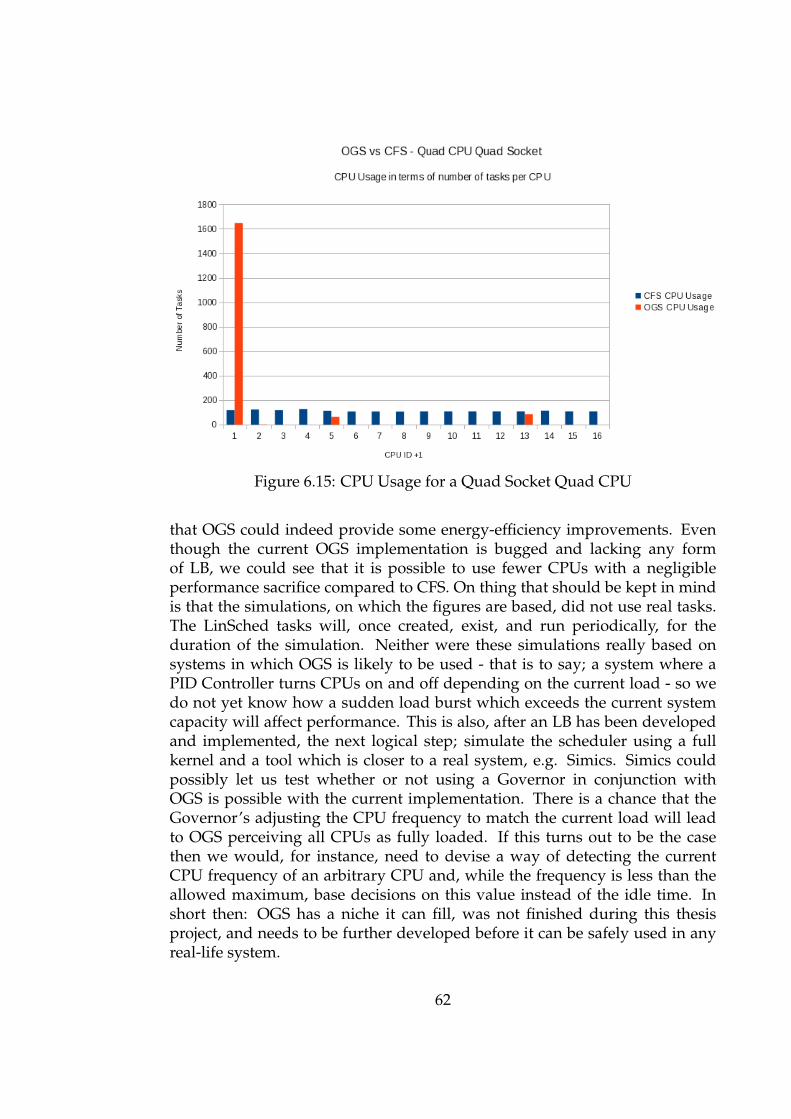
Figure 6.15: CPU Usage for a Quad Socket Quad CPU
that OGS could indeed provide some energy-efficiency improvements. Eventhough the current OGS implementation is bugged and lacking any formof LB, we could see that it is possible to use fewer CPUs with a negligibleperformance sacrifice compared to CFS. On thing that should be kept in mindis that the simulations, on which the figures are based, did not use real tasks.The LinSched tasks will, once created, exist, and run periodically, for theduration of the simulation. Neither were these simulations really based onsystems in which OGS is likely to be used - that is to say; a system where aPID Controller turns CPUs on and off depending on the current load - so wedo not yet know how a sudden load burst which exceeds the current systemcapacity will affect performance. This is also, after an LB has been developedand implemented, the next logical step; simulate the scheduler using a fullkernel and a tool which is closer to a real system, e.g. Simics. Simics couldpossibly let us test whether or not using a Governor in conjunction withOGS is possible with the current implementation. There is a chance that theGovernor’s adjusting the CPU frequency to match the current load will leadto OGS perceiving all CPUs as fully loaded. If this turns out to be the casethen we would, for instance, need to devise a way of detecting the currentCPU frequency of an arbitrary CPU and, while the frequency is less than theallowed maximum, base decisions on this value instead of the idle time. Inshort then: OGS has a niche it can fill, was not finished during this thesisproject, and needs to be further developed before it can be safely used in anyreal-life system.
62
CHAPTER
SEVEN
FURTHER WORK
This chapter will list OGS issues and problems that have been identified, buthave yet to be solved. It will also list what is not so much issues with thescheduler, but rather functionality that has yet to be implemented.
• Test in a full-kernel simulator. E.g. Simics.
• Get a concrete measurement of power consumption when using OGS,and OGS in its intended role as a part of the PID PM.
• Implement and test OGS LB as proposed
– Add struct elements relevant to OGS LB to struct sd_lb_stats. Putthem behind #ifdefs with conditions ensuring they are only built inand used when OGS is the scheduler of choice.
– Add struct elements relevant to OGS LB to struct sg_lb_stats. Putthese elements behind #ifdefs as well.
– Change update_sd_lb_stats() in order to update the struct elementsrelevant to OGS LB.
– Change update_sg_lb_stats() in order to update the struct elementsrelevant to OGS LB.
– Develop alternative to find_busiest_group(). Call it find_idlest_group()or similar.
– Identify scenarios for OGS where an imbalance does not exist fromthe point of view of this_cpu.
63

– Change find_busiest_queue() to find_idlest_non_idle() or similar.
– Change the calculations in calculate_imbalance() to the ones sugges-ted in Subsection 4.2.3.
– Verify that everything works as intended, without changes, frommove_tasks() all the way to the end of the LB procedure chain.
– Solve the fallback problem. Potentially solveable by letting CFSchoose a RQ among the ones that are not in a Sleep State.
• Develop, implement, and test a scheme which detects potential over-loads. We can currently only detect if a CPU has an idle time of naught,but are unable to detect if the load actually exceeds the capacity. Onepotential solution would be to add a metric akin to a soft deadline toevery task, which would detect how long a task has to wait for CPUtime. If the average detected waiting time for the whole RQ on exceeds acertain threshold, then the RQ would be flagged as overloaded.
• Confirm whether or not using a Governor in conjunction with OGS willmuddle the idle_time readings. If this turns out to be the case, then figureout if polling the current CPU frequency is a solution.
64

CHAPTER
EIGHT
CONCLUSION
The premise for this thesis was the use of a PID controlled power managerto improve the energy efficiency of a Linux-driven cloud system. We coveredsome basic Control Theory relating to PID controllers and explained how itrelates to the proposed PID power manager. We also quickly covered how thepower manager is meant to work in terms of how it will influence the system toachieve the control objectives. This is necessary as the work performed hereinwill be an autonomous extension of the aforementioned power manager in acloud system.
We investigated the Linux kernel with the intention to identify any potentiallypre-existing and implemented functionality related to energy efficiency. Somefunctionality was found to already be in place and its suitability for ourplanned implementation was evaluated. We found it to be insufficient for ourpurposes and hence a number of changes were proposed. The changes requirethe kernel code to be tweaked, therefore we isolated the code related to thechanges we have proposed, and explained in detail how it works in the currentkernel. Then we went on to explain how we want to implement our proposedchanges as well as giving a detailed explanation of the changes already putin place both in terms of code and in terms of intended functionality. Not allof the proposed changes were implemented during this thesis project, and wehave pointed out which ones are still missing. The proposed changes amountto a new scheduler we have decided to call the Overlord Guided Scheduler.
While the implementation is currently incomplete, it is possible to runsimulations using what is already in place and compare the results against an
65
existing scheduler. All results were gathered from simulations using simulatedsystems. None of the resuts are from real-life cases, as the proposed schedulerwould have to be complete before it can be safely used in such cases. Theresults were produced for a number for different architectures and parameters,and analysed in Excel on a per-architecture and parameter set basis. Weshowed that OGS can provide improvements to energy efficiency comparedto CFS. OGS used fewer CPUs in all cases, and often with a negligible dropin performance. The simulations also showed that OGS is not quite complete,and illustrated a few issues that had not been considered, but are now listedunder Further Work. The conclusions drawn from these results indicate thatthe proposed scheduler requires more work, but are otherwise promisingwith regards to energy efficiency. At the time of writing we are unable toproduce concrete results regarding the actual energy efficiency of a cloudsystem employing a PID controlled power manager assisted by the proposedscheduler.
66

BIBLIOGRAPHY
[1] Efficient servers, a project conducted within the eu-programme intelligentenergy europe. Online.
[2] Free electrons linux cross reference - arch/x86/kconfig. Accessed:September 14 2011.
[3] Free electrons linux cross reference - kernel/sched_fair.c. Accessed:October 25 2011.
[4] Materials modification inc. Accessed: September 26 2011.
[5] Tomoyo linux cross reference - sched.c. Accessed: September 7 2011.
[6] Tomoyo linux cross reference - sched_fair.c. Accessed: September 7 2011.
[7] Tomoyo linux cross reference - sched_fair.c, alb. Accessed: September 142011.
[8] Linux kernel newbies, April 2007. Accessed: September 9 2011.
[9] Cacti documentation and howtos, May 2010. Accessed: September 192011.
[10] B. Przywara T. Bogner S. Weeren B. Schäppi, F. Bellosa and A. Anglade.Energy efficient servers in europe, energy consumption, saving potentials,market barriers and measures. Part 1: Energy consumption and savingpotentials. The Efficient Servers Consortium, Tech. Rep., November 2007.
[11] Simon Holmbacka. Task migration in virtualized multi-core real-timesystems. Master’s thesis, Abo Akademi University, 2010.
[12] Jenifer Hopper. Reduce linux power consumption, part 1: The cpufreqsubsystem. September 2009.
67

[13] Jenifer Hopper. Reduce linux power consumption, part 3: Tuning results.October 2009.
[14] M. Tim Jones. Inside the linux 2.6 completely fair scheduler. December2009.
[15] M. Tim Jones. Linux scheduler simulation. Febuary 2011.
[16] Avinesh Kumar. Multiprocessing with the completely fair scheduler.January 2008.
[17] U. Holze L. Barroso. The case for energy-proportional computing.Computer, 40(12):33–37, December 2007.
[18] Suresh Siddha, Venkatesh Pallipadi, and Arjan Van De Ven. Gettingmaximum mileage out of tickless. Proceedings of the Linux Symposium,2:201–207, 2007.
[19] Johan Lilius Simon Holmbacka, Sebastien Lafond. Power proportionalcharacteristics of an energy manager for web clusters.
[20] Johan Lilius Simon Holmbacka, Sebastien Lafond. A pid-controlledpower manager for energy efficient web clusters. In Proceedings of theInternational Conference on Cloud and Green Computing (CGC2011), 2011.
[21] Olle Svanfeldt-Winter. Energy efficiency of arm architectures for cloudcomputing applications. Master’s thesis, Abo Akademi University, 2011.
68

SWEDISH SUMMARY
ENERGIEFFEKTIV SCHEMALÄGGNING FÖR MOLNSY-STEM
Introduktion
En snabbt växande befolkning har lett till ett allt större behov av elektricitet,medan en ökande miljömedvetenhet sätter allt högre krav på energieffektiviteti exempelvis datorsystem. För att inte tala om att en lägre strömförbrukning ärmer ekonomisk.
Eftersom internet och dess användning sakta går mot att bli allestädes närva-rande ökar även kraven på de bakomliggande serversystemen. Ju mer kravenökar, desto mer måste systemen utökas för att kunna möta kraven. Härav följeratt ju större serversystemen blir, desto större blir deras strömförbrukning.Eftersom dessa system förbrukar en ansenlig mängd elektricitet även då deinte är fullt belastade, så är det inte hållbart i det långa loppet att enbart utökaderas kapacitet. Detta beror delvis på att serversystemens strömförbrukninginte är proportionell mot den momentana belastningen och det är dettaproblem det här arbetet kommer att undersöka.
Detta arbete kommer till en viss mån att bygga på och vidareutveckla ett arbeteutfört av en annan studerande här vid Åbo Akademi [11]. Detta arbete äräven utfört som en del av ett forskningsprojekt, vars målsättning är att utredamöjligheterna att bygga energieffektiva processorkluster av strömsnåla mo-bilprocessorer. Syftet med detta arbete är att utreda linuxkärnans lämplighetför en tillämpning inom ett system som använder sig av en PID-regulator föratt kontrollera strömförbrukningen. Förändringsförslag ges i det fall kärnansnuvarande funktionalitet uppfattas som otillräcklig eller olämplig.
69

Schemaläggning och strömförbrukningshantering iden nuvarande Linuxkärnan
Utvärderingen av Linuxkärnan påbörjas med en undersökning av de tillgäng-liga schemaläggarna och deras funktionalitet. I princip finns det i dagslägetbara två schemaläggare i kärnan, eftersom den gamla O(1)-schemaläggarenhelt ersatts med Completely Fair Scheduler (CFS). Den andra schemaläggareni kärnan är realtidsschemaläggaren, som, vilket namnet antyder, sköterschemaläggning i realtid. Eftersom realtidsschemaläggning inte är av intressei det här skedet kommer fokus att ligga på CFS.
CFS kan konstateras besitta en mängd önskvärda egenskaper. Den har tillexempel gjort sig av med den diskreta körtidsindelningen som de tidigareschemaläggarna använt sig av, vilket förminskar tiden en processor (CPU)vilar i onödan för att en exekvering inte fyller hela körtidsindelningen. CFShar också gjort sig av med körköer och använder sig istället av ett röd-svartträd"(RBT). Trädet är sorterat enligt i hur stort behov en process är av att fåtillgång till processorn. Då ett program fått köra uppdaterar det sin körtid ienlighet med hur lång denna tid var och, i det fall det fortfarande är i behovav körtid, läggs sedan tillbaka i trädet. Eftersom trädet är självsorterandekommer den nyligen exekverade processen att flyttas till det ställe i trädet sommotsvarar dess nya körtidsbehov. På detta sätt håller schemaläggaren enkeltkoll på vilken process som bör köras till näst.
Då en ny process har skapats måste schemaläggaren bestämma i vilken körkö(RQ) - egentligen RBT, men de kommer för enkelhetens skulle att kallas förkörköer här - och i förlängningen vilken CPU processen ska köras på. I CFSsköts detta av några funktioner vars uppgift är att hitta den minst belastadeRQ:n i den minst belastade schemaläggningsgruppen (SG). Den planeradelösningen kräver en schemaläggare som kan fylla RQ:na sekventiellt. Detvill säga en schemaläggare som lägger nya uppgifter till samma RQ tillsdenna har nått sin kapacitet. För att detta ska vara möjligt måste en övrebelastningsgräns definieras för varje körkö. CFS mäter belastningen i "viktadarbetsbörda", vars exakta funktionalitet ligger gömd bakom ett flertal lagerkärnkod. Den använder sig inte heller av en belastningsbegränsning påett för den tilltänkta lösningen lämpligt sätt. Att förändra CFS beteendeså det matchar kraven skulle kräva en grundlig utredning av den viktadearbetsbördans funktionalitet. Då en utredning av denna funktionalitet skulleha tagit längre än tiden tilldelad detta projekt, gjordes ett beslut att undersökamöjligheterna hur ett alternativt sätt att välja SG och RQ kunde tillämpas.
Eftersom så gott som alla processer är ändliga kommer både antalet och för-delningen av dem att förändras medan ett system körs. I de fall ett system har
70

flera CPU:n blir det således önskvärt att efter en viss tid balansera belastningen(LB) för att undvika att en enskild CPU hanterar hela belastningen. I CFS görsdetta genom att man periodiskt söker efter den mest belastade RQ:n i denmest belastade SG:n, varifrån processer sedan flyttas till den RQ vars CPUgör LB just nu. Målsättningen är alltså att alla RQ:n ska ha ungefär sammabelastning, så i det fall det visar sig att CPU:n som gör LB just nu är merbelastad än medelbelastningen kommer processflytten att skippas. Att fördelabelastningen jämnt över alla RQ:n passar inte den tilltänkta tillämpningen. Enidealisk LB skulle här se till att möjligast få CPU:n är i användning utan attvara överbelastade, så vissa förändringar krävs även här.
Linux är dock inte helt oanvändbart i sin nuvarande tappning. En användbarfunktionalitet som redan finns är de så kallade Guvernörerna (Governors).Då de är i användning ser de till att CPU-frekvensen är proportionell motden momentana arbetsbördan. Även om pluralformen för guvernör användshär bör det antas att det är en samlingsterm, då endast en guvernör kananvändas åt gången, men fungerar i mångt och mycket på samma vis somde andra guvernörerna. Att justera frekvensen i förhållande till arbetsbördanleder vanligtvis till att en CPU förbrukar en mindre mängd ström medanden fortfarande till synes sköter sina uppgifter lika fort och smidigt. För attåstadkomma detta håller guvernörerna koll på hur länge en CPU exekverarnågot och hur länge den vilar och sparar dessa värden i en struktur.Dessa värden kontrolleras med ett godtyckligt samplingsintervall och omvilotiden är längre än ett godtyckligt tröskelvärde konstaterar guvernörenatt frekvensen kan sänkas. Höjningen av frekvensen sköts i omvänd ordning[14][16][5][6][8][18][7][2][13][12][9].
Kontrollerad strömförbrukningshantering
PID-regulatorer förknippas vanligen med ett maskineri eller dylika konceptdär det finns något konkret och uppenbart att kontrollera. Farthållaren ien bil t.ex. använder sig av en regulator, vars uppgift det är att ta denönskade hastigheten som referensvärde och använda detta i samband med dennuvarande hastigheten för att beräkna hur mycket gasreglaget bör justeras föratt uppnå målsättningen.
Om man förenklar något kan man säga att en PID-regulator löser en andragradens differentialekvation med avseende på ett felvärde. Felvärdet ärdifferensen mellan referensvärdet och det nuvarande uppmätta värdet. I fart-hållarexemplet är referensvärdet den önskade hastigheten och det uppmättavärdet är den resulterande hastigheten. Utgående från detta fås:
71

y = Ki
∫ t
0
e(τ)dτ +Kpe(t) +Kdd
dte(t) (8.1)
där y är utvärdet till farthållaren, e() är felvärdet - e = r − y där r ärreferensvärdet - och K är förstärkningskonstanter specifika för de enskildaoperationerna i ekvation 8.1.
Det planerade serversystemet med en PID-regulator som ansvarar för ener-gieffektiviteten kommer, om allt visar sig fungera planenligt, att kontrollerahur många CPU:n som är påslagna. Regulatorn tar antal förfrågningar somreferensvärde och använder detta för att beräkna hur många CPU:n sombehövs för att möta den resulterande belastningen. Om det visar sig behövasfärre CPU:n stänger regulatorn av så många vilande CPU:n som beräkning-arna säger är överopps. Om det visar sig behövas fler CPU:n kommer ettmotsvarande antal CPU:n att startas upp. Denna procedur har redan visatsvara 30 till 80 % mer energieffektiv än de existerande procedurerna [19].
Schemaläggningsrelaterade förändringsförslag
Den existerande schemaläggaren, CFS, är alltså inte lämplig för den planeradetillämpningen tillsammans med en PID-regulator. Dess algoritm för RQ-valoch dess LB-procedur måste ändras. Inom loppet av detta arbete fanns baratid för att implementera en ny algortim för RQ-val. Denna förändring harympats in i kärnkoden på de för syftet relevanta ställena. På så vis har konceptsom låsning inte behövts tas i beaktande, då de redan är fungerande och finnspå plats. Förändringarna påverkar således enbart vilket CPU ID-nummer somreturneras från RQ-valsalgoritmen. Dessa förändringar kommer hädanefter attkallas Overlord Guided Scheduler (OGS).
För att välja RQ i enlighet med kraven bör OGS ha koll på belastningen i varjeenskild CPU. Lyckligtvis behöver detta inte skapas skilt, utan det är möjligtatt använda sig av samma information som guvernörerna samlar in. Dennainformation inkluderar alla bidrag till exekveringstid på en CPU, vilket gördet möjligt att utgående från detta fatta ett beslut om huruvida en CPU är fulltbelastad eller inte. En fullt belastad CPU kommer inte att ha någon vilotid,medan en CPU med tillräckligt stor vilotid kan hantera fler processer. OGSkommer alltså att schemalägga nya processer på samma CPU tills dess vilotidär så gott som noll.
Belastningsbalanseringen är i skrivande stund inte klar och implementeradännu, men det finns dock en idé om hur detta kunde lösas. LB-procedurens
72

beslut kommer att basera sig på samma information som RQ-valen. Proce-duren håller koll på vilken RQ som är mest belastad, men med kvarvarandekapacitet, samt vilken RQ som är minst belastad. I mån av möjlighet flyttas såmånga processer som den mest belastade RQ:n kan hantera från den minstbelastade. Då denna procedur utförs periodiskt kommer antalet belastadeCPU:n att hållas möjligast litet.
Sätten som RQ-valsalgoritmen och LB-proceduren fungerar på är relativtviktiga för att PID-regulatorn ska kunna utföra sitt jobb obehindrat. Då dessprimära uppgift delvis består av att stänga av vilande CPU:n är det viktigtatt enstaka processer inte exekveras på en CPU här och en CPU där. OGS hardärför som uppgift att assistera regulatorn genom att samla alla processer isystemet på möjligast få CPU:n utan att offra alltför mycket i form av uppfattadprestanda.
Verktyg, experimentation och testning
Eftersom schemaläggning är ett av de mest komplexa koncepten i linuxkärnanoch ett av de mer kritiska ur en prestandasynvinkel, är det otroligt utmanandeatt skriva en felfri schemaläggare. Tar man ännu installerings- och byggtidenför en ny kärna i beaktande kommer man ganska fort fram till att detta inte ärnågot man gärna gör direkt i systemet man för tillfället använder. Till all lyckafinns det nuförtiden verktyg som LinSched.
LinSched tar sig runt de ovan nämnda problemen genom att migrera sche-maläggningssubsystemet till "user space". På så sätt är det i princip möjligt attköra tester på den planerade schemaläggaren i något av en nerbantad virtuellkärna. LinScheds version av kärnan saknar dock en hel del funktionalitet ochverifierar t.ex. inte låsning, så schemaläggaren måste ändå i något skede testasi en full kärna, men på det här sättet kraschar man inte hela maskinen om mangjort ett fel.
En för OGS viktig funktionalitet visade sig saknas i LinSched-kärnan, nämli-gen informationen som guvernörerna bidrar med. För att komma runt dennabegränsning lades falska uppdateringar, som bidrog med exekveringstiderför processorerna, till i LinScheds källkod. Detta innebar att informationenpå vilken OGS baserade sina RQ-val inte var helt korrekt, men det varåtminstone möjligt att verifiera dess beteende och efter lite finjusteringar ävenatt jämföra dess prestanda med CFS. En annan funktionalitet som saknadesvar systemtiden. Både OGS och guvernörerna använder sig av denna för atthålla koll på hur lång tid som förflutit sedan det senaste beslutet gjordes. Dettalöstes genom att plocka in systemtiden från den egentliga kärnan.
73

Simuleringarna kördes sedan för fem olika topologier med ett stort antal olikasimuleringsparametrar för både CFS och OGS. Resultaten jämfördes sedan iExcel för de olika topologierna och parametrarna. Utgående från dessa gjordessedan ett antal beräkningar, vilkas resultat ritades som grafer för att enklarevisualisera dem. I dessa grafer jämfördes exekverings- och fördröjningstider,processorernas allokeringsordning, antal processer per CPU, skillnaden iexekveringstid per process samt exekveringstidskvoterna per process.
Då simuleringarna inte skedde i verkliga system kunde strömförbrukningeninte mätas och jämföras för schemaläggarna. För att kunna göra en approxi-merad jämförelse av de två gjordes antagandet att varje belastad CPU innebären konstant förbrukning på 10 W.
Resultat
I resultaten kunde påvisas att OGS i alla fall använder färre CPU:n än CFS.OGS påvisar dock även ett antal buggar samt att LB fortfarande saknas. Dådetta tas i beaktande kan man konstatera att om dessa resultat gäller även i enfull implementation i en komplett kärna, så är OGS mer energieffektiv än CFSmed en mycket liten negativ inverkan på prestanda.
Vidare arbete
Som det har nämnts ett antal gånger är OGS inte klar än. En del funktionalitetsaknas och en del borde ännu kontrolleras efter buggar och alltihop bordetestas i en simulator som t.ex. Simics som kan utnyttja en full kärna. Det hittillsidentifierade behovet av vidare arbete är:
• Testa schemaläggaren i en full kärna.
• Lägg upp ett test där den faktiska strömförbrukningen kan mätas.
• Implementera resten av OGS och testa detta.
• Utveckla, implementera och testa ett sätt att upptäcka möjliga över-belastningar. Dessa kan ske om en process visar sig kräva en längreexekveringstid än uppskattat.
• Utred och testa huruvida användningen av en guvernör i samband medOGS fungerar med de nuvarande algoritmerna. Det finns en möjlighet
74

att guvernörens justeringar av CPU-frekvensen leder till att OGS fårfelaktiga värden.
Slutsats
Detta arbete har baserats på idén att en PID-reglerad strömförbruknings-hantering kan användas för att förbättra energieffektiviteten i ett linuxdrivetmolnsystem. Grundläggande reglertekniksteori relaterad till PID-regulatorerförklarades samt sambandet mellan denna teori och den planerade ström-förbrukningshanteringsregulatorn. Hur regulatorn ska nå sin målsättning haräven förklarats, vilket är nödvändigt eftersom OGS kommer att fungerasom en autonom förlängning av strömförbrukningshanteringsregulatorn i ettmolnsystem.
Linuxkärnan har undersökts med målsättningen att identifiera existerandeströmsnålhetsfunktionalitet. En del funktionalitet kunde identifieras ochdess lämplighet för den planerade implementationen evaluerades. Funk-tionaliteten konstaterades vara otillräcklig och olämplig för den planeradeimplementationen och därför krävdes och föreslogs ett antal förändringar.Dessa förändringar kräver justeringar av vissa algoritmer, så den relateradekärnkoden isolerades och dess funktion förklarades. Därefter förklarades hurde föreslagna förändringarna planerats fungera och hur de är implementeradejust nu. Alla förändringar har inte implementerats i skrivande stund, men ävende utelämnade förändringarna nämdes. Förändringarna kommer att resulterai en ny schemaläggare som kommer att kallas Overlord Guided Scheduler.
Även om implementationen för tillfället inte är fullbordad var det möjligt attköra simulationer med den funktionalitet som finns på plats och att jämförade producerade resultaten med den existerande schemaläggaren. Inga resultathar i det här skedet producerats med en full kärna på ett verkligt system,då schemaläggaren bör vara fullständig förrän den kan användas i ett dyliktsystem. Slutsatserna dragna från de producerade resultaten är att OGS verkarkunna förbättra energieffektiviteten i Linux, men att en mängd arbete kvarstårförrän schemaläggaren kan påstås vara fullständig och klar för en verkligtillämpning. Problem och fortsatt arbete har listats i kapitlet om framtidaarbete.
75

APPENDIX
A
LINUX KERNEL CHANGE LOG
In file:kernel_source_code/arch/x86/Kconfig
- Added config option and other relevant bits for Overlord.- Option is dependent on SMP, as it is pointless in systems
with only one cpu- Default choice is N- Also added a quick help desciption
- The same thing should be added in all arch-related Kconfigs
In file:sched.c
- Put other OGS-related definitions, i.e. those not of the formabove, behind an #ifdef for the same reasons
- Added files to the include list- stdio.h for print functions- linux/fake_kstat.h in case we need the fake time
accounting here (behind #ifdef)
- Option to print location from various functions in order tokeep track of where we are.- #ifdef PRINT_LOCATION in:
76

- schedule()- scheduler_tick()- resched_task()- set_task_rq()- __set_task_cpu()
- Option to print capacity- #ifdef PRINT_CAPACITY in:
- schedule()- Prints the returned CPU’s ID and its idle time
- Option to turn off load balancing- #ifndef NO_LOAD_BALANCE- Removes trigger_load_balance(), i.e. the first function
in the LB chain, at compilation time
- Added functions: update_fake_*_time()- Updates the faked busy time accounting- Updates parts of the struct in fake_kstat.h depending on
which of the functions we’re calling- Most of the updates use a static and arbitrary number- update_fake_busy_time uses the sum_exec_runtime value
to give us something that varies- ((struct task_struct*)current)->se.sum_exec_runtime- This is the same runtime value linsched uses in its reportingfunction- Called from:
- wake_up_new_task()- try_to_wake_up()
In file:sched_fair.c
- Added #ifdefs to various places to make swapping between CFSand OGS easier- CONFIG_SCHED_OLORD- CONFIG_OLORD_GROUP_SCHED- In most cases we use the CFS code in this file
- Added #ifdefs for when linsched is no longer used
- Added files to the include list
77

- stdio.h for print functions- linux/fake_kstat.h in case we need the fake time
accounting here (behind #ifdef)
- Added definition of a struct array- struct colonel_stat cstat[LOTS]- Used for busy time accounting
- LOTS = 100, defined in fake_kstat.h
- Added functions: update_fake_*_time()- Updates the faked busy time accounting- Updates parts of the struct in fake_kstat.h depending on
which of the functions we’re calling- Most of the updates use a static and arbitrary number- update_fake_busy_time uses the sum_exec_runtime value
to give us something that varies- ((struct task_struct*)current)->se.sum_exec_runtime- This is the same runtime value linsched uses in itsreporting function- THESE FUNCTIONS WERE MOVED TO SCHED.C
- Now in:- wake_up_new_task()- try_to_wake_up()
- Added function: what_is_idle_time()- Calculates the amount of idle time on a CPU.- Uses the struct available in include/linux/kernel_stat.h
- This struct is also used by the governors- All update functions for this struct should be included in theoriginal kernel code- If we’re using linsched then the struct is "faked" as the
update functions do not works- Use the update_fake functions mentioned above to keep track ofthe idle time
- Does not correspond entirely to reality- Changed the CPU ID check
- We need one as the cpu value is an unsigned int in some places- If the ID is out of range, return idle time = 0 which willexclude the CPU from the search- This is a temporary solution
- Added function: find_busy_group()- Finds the busiest scheduling group with enough idle time
78
to be able to accommodate new tasks- For more details see the function- Changed how the SAFETY_MARGIN is noted
- We now have a separate variable here, which is incrementedby one SAFETY_MARGIN per group member
- Added function: find_busy_sched_cpu()- Finds the busiest cpu with enough idle time to be able to
accomodate new tasks- Calculates the average busy time contribution per task on
the runqueue to figure out if adding another task is likelyto cause an overload
- For more details see the function
- Option to print location from various functions in order tokeep track of where we are- #ifdef PRINT_LOCATION_FAIR in:
- select_task_rq_fair()- find_busy_sched_cpu()- run_rebalance_domains()- rebalance_domains()- move_tasks()- balance_tasks()
- Option to print capacity- #ifdef PRINT_CAPACITY
- Option to print cpu choice- #ifdef PRINT_CHOICE
- Added fake time accounting to select_task_rq_fair- This is to make sure we actually update the kernel stats
when a test is run- It may turn out we account for the time twice when running
a simulation, although this is not really a problem sinceit should mean we need to use another cpu quicker which inturn makes it easier to see if everything works as intended
- Edited structure sd_lb_stats- Uses original structure when Overlord is not used- Uses elements with the same name for Overlord, but they
are now of type cputime64_t- If we’re using Linsched, they’re still unsigned longs, but put
79

inside their own #ifdefs in case we have to change something- Added elements when using Overlord
- total_idle, for tallying the total idle time for all groupsin the SD
- this_idle, for tallying the idle time for this group- unsigned longs when using Linsched, cputime64_t else
- Edited structure sg_lb_stats- Uses original structure when Overlord is not used- Uses elements with the same name for Overlord, but they
are now of type cputime64_t- If we’re using Linsched, they’re still unsigned longs, but putinside their own #ifdefs in case we have to change something
- Added CONFIG_SCHED_OLORD as an alternative condition beforeinit_sd_power_savings_stats- We always want to use this with Overlord
- Changed conditional in: update_sd_power_savings_stats- If the local group is idle or completely loaded, then
there is no need to do power savings balance at thisdomain.
- For Overlord, the capacity is measured in idle time and NOThow many tasks we’ve running. Thus the comparison is nowperformed against this_load instead of this_nr_running
- Edited function in: update_sd_power_savings_stats()- #ifdef conditional for Overlord- Inside #ifdef:
- Changed conditionals so they now look at and updateaccording to idle time. Was based on nr_runningpreviously.
- The function contains what is essentially two sets ofsimilar conditions and value edits.This is because it makes the code easier to read and the#ifdef gets rid of the part we’re not using duringcompilation.
- Edited function in: update_sg_lb_stats()- Again, added a copy of this function’s internals for
Overlord, which was subsequently edited- Usage governed by #ifdefs- Removed the local group bias
80

- Changed the load calculation to what_is_idle_time() fromtarget_load()
- Removed the update related to weighted_cpuload(). We don’tuse it anyway
- sgs->group_capacity is now calculated in the for-loop- Removed a calculation adjusting the load by the relative
CPU power of the group.- Removed a call to update_group_power(). Does nothing
relevant at this point.- Group imbalance is flagged if:
- min_cpu_load can fit in max_cpu_capacity- max_cpu_capacity is larger than avg_load_per_task- Add more cases?
- Added printf() after the for-loop to check if we can use"i" from the loop-variables
- If a usable value for NR_CPUS exists, then "i" could beset = NR_CPUS+1
- Edited function in: update_sd_lb_stats()- Again, added a copy of this function’s internals for
Overlord, which was subsequently edited- Usage governed by #ifdefs- Removed : sds->total_pwr+= group->cpu_power
we’re not likely to use it- Changed some values *this will get
- sds->this_load = sgs.avg_idlefrom: sds->this_load = sgs.avg_load
- sds->this_load_per_task = sgs.avg_load_per_taskfrom: sds->this_load_per_task = sgs.sum_weighted_load
- Smaller this_load values now mean a higher load. May yet changethe name of the struct element to this_idle- Changed some values *busiest will get
- sds->max_load = sgs.avg_idlefrom: sds->max_load = sgs.avg_load
- sds->busiest_load_per_task = sgs.avg_load_per_taskfrom: sds->busiest_load_per_task = sgs.sum_weighted_load
- Smaller max_load values now mean a higher load. May yet changethe name of the struct element- Changed conditions for setting the *busiest values
- Now: sgs.avg_idle < sds->max_load &&(sgs.group_capacity < SAFETY_MARGIN || sgs.group_imb))
- Before: sgs.avg_load > sds->max_load &&(sgs.sum_nr_running > sgs.group_capacity || sgs.group_imb))
81

- Purpose: Have the busiest group be one that is overloaded,where *group_leader is a busy NON-OVERLOADED group.
This should mean we can up performance a bit, while stillmaintaining power efficiency
- Edited function in: fix_small_imbalance()- Again, added a copy of this function’s internals for
Overlord, which was subsequently edited- Usage governed by #ifdefs- Removed variable inits from the original function. Turned
out they weren’t needed- Removed the init calculations from the original function.
Turned out they weren’t needed- *imbalance is now set if:
- max_load is less than SAFETY_MARGIN and this_load is largeenough to fit at least one task from busiest- max_load and this_load are reported in terms of idle time
- this_load could fit at least one task from min_load- By leeching tasks off the least loaded every chance we get
should lead to our being able to put more cpus to sleep
- Edited function in calculate_imbalance()- Again, added a copy of this function’s internals for Overlord, which was subsequently edited- Usage governed by #ifdefs- Removed averaging of busiest_load_per_task. It already IS
an average.- if (sds->group_imb) does nothing at the moment- if (!sds->group_imb) changed:
- Sees if busiest is overloaded and if so; calculates the amount- Sets load_above_capacity = 0 if busiest is not overloaded
- Changed the way *imbalance is determinedwe should pull from the target.
- We see if busiest is not overloaded and calculate the number oftasks we could pull to it
- We calculate the number of tasks we could pull to leader- If we can pull 1 or more tasks to busiest, do it- If we cannot pull to busiest, but can pull 1 or more tasks to
leader, do it- Otherwise, pull to this- If busiest turned out to be overloaded, just check leader and
this to see how much to pull- Make sure imbalance is at least 1
82

- If not, then try fix_small_imbalance()- On returning from this function,
*imbalance = NUMBER OF TASKS TO PULL- Commented scenario that seemed to be specific for CFS
- if (sds->max_load < sds->avg_load)
- Edited function in find_busiest_group()- Removed conditions for when imbalance does not exist from
the POV of this_cpu- Imbalance is within the specified limit- There is no busy sibling to pull from- This group is more busy than the average business at thissched_domain- New (and re-used) conditions for when imbalance does not
exist from the POV of this_cpu- this_cpu is not the appropriate cpu to perform load balancingat this level
- This group is the idlest group- This group is hte busiest group and can’t take on any new tasks- Busiest is not Overloaded
- Edited function in check_power_save_busiest_group()- Again, added a copy of this function’s internals forOverlord, which was subsequently edited
- Usage governed by #ifdefs- Introduced variable int power_save_pull
- The number of tasks we can pull from busiest or idlest- Integer so we don’t have to worry about rounding- Never greater than the number of tasks running on the
target queue
- Changed conditions for returning 0. We return 0 if:- If this != group_leader- If group_leader = group_min- If leader can’t take on any more tasks
- Changed what is due to happen if we return 1.- If busiest_group_capacity > SAFETY_MARGIN (i.e. is not
overloaded)- Calculate how many tasks we can pull from group_min to leader- Make sure we don’t try to pull more than min_nr_running- Set sds->busiest = sds->group_min (because the balancinglogic always pulls from busiest)
- If busiest_group_capacity < SAFETY_MARGIN (i.e. IS
83

overloaded)- Calculate how many tasks we can pull from busiest to leader- Make sure we don’t try to pull more than busiest_nr_running(this shouldn’t be possible)
- Just return 1, since sds-> busiest already points at thequeue we want to pull from
- Edited function in find_busiest_queue- Again, added a copy of this function’s internals forOverlord, which was subsequently edited
- Usage governed by #ifdefs- Added variable time_now
- For Linsched type = unsigned long- Else type = cputime64_t
- Removed variable power- Changed values for:
- Capacity now it is = what_is_idle_time(cpu, time_now)- Workload (wl) now it is = time_now - capacity
- Changed conditions for skipping to the next increment- If nr_running < 2 :: continue
- This is because an RT-task might use loads of CPU time, butmoving it somewhere else, would not improve on anythingNot to mention that its extremely high avg_load_per_taskvalue would most likely mean no RQ can take it
- Edited function in load_balance()- Added printf to see when we end up in this function
- Usage governed by #ifdef
- Edited function in load_balance_fair()- Again, added a copy of this function’s internals forOverlord, which was subsequently edited
- Usage governed by #ifdefs- Added printf to see when we end up in this function
- Usage governed by #ifdef- Removed calculation update_h_load(busiest_cpu)
- Do not need/use it- Removed calculation rem_load * busiest_weight &
div_u64(rem_load, busiest_h_load + 1)- Do not need/use it
- Removed calculation moved_load * busiest_weight &div_u64(moved_load, busiest_h_load + 1)- Do not need/use it
84

- Changed variable type- u64 to unsigned long for rem_load- u64 to unsigned long for moved_load
- Edited function in balance_tasks()- Added a copy of most of the function’s parts.
- Only had to change the bits relating to the moved loadat the start of the loop
- Usage governed by #ifdef- Change conditions for invoking continue
- Not using load weights, so no point in having(p->se.load_weight >> 1) > rem_load_move
- Now only invoked if !can_migrate_task()- Change decrement of rem_load_move
- Now decremented by 1, since *imbalance is in number oftasks to move
In file:fake_kstat.h
- New file- Placed in /include/linux
- Emulates the necessary parts of kernel_stat.h- Contains the busy time accounting function prototypes
In file:sched.h
- Added #ifdefs to make swapping between CFS and OGS easier- CONFIG_SCHED_OLORD- CONFIG_OLORD_GROUP_SCHED
- No big changes here. We use CFS-code in all cases
85

APPENDIX
B
LINSCHED CHANGE LOG
In file:Makefile
- Added definition flags for OGS- -D CONFIG_SCHED_OLORD- -D CONFIG_OLORD_GROUP_SCHED
In file:basic_tests.c
- Added #ifdefs to various places to make swapping between CFSand OGS easier
- Added ridiculously lax result validation requirements to alltests
- Added the result printing function to all tests. They are nowprinted regardless of the outcome- linsched_print_task_stats()
- In test_trivial_bal()- Task creation is now in a for-loop- We create one task at a time and run it for 5ms- We create one task per cpu- The test is then run for an additional
(TEST_TICKS-(count*5))ms- Creating tasks like this will give the kernel stats a
chance to update before the next task is created- In test_basic_bal1()
- A similar change to task creation
86

- Create 5 sleep/run tasks and run sim for 500ms- Do this for each CPU- Run the test to its conclusion, i.e.
(TEST_TICKS-(count*500))ms- This gives us quite a few tasks to schedule, but fewer
than we’d need to fill up all cpus (I think), whichshould help in identifying potential problems
- In test_basic_bal2()- A similar change to task creation- Create 5 sleep/run tasks and run sim for 500ms- Do this for each CPU- Run the test to its conclusion, i.e.
(TEST_TICKS-(count*500))ms- This gives us quite a few tasks to schedule, but fewer
than we’d need to fill up all cpus (I think), whichshould help in identifying potential problems
- In test_bal1()- A similar change to task creation- Test includes cpu-bound tasks, so create these first and
run for 100ms- Overlord does not take cpu affinity into consideration at thispoint- Create 5 sleep/run tasks and run sim for 500ms- Do this for each CPU- Run the test to its conclusion, i.e.
(TEST_TICKS-(count*500)-100)ms- This gives us quite a few tasks to schedule, but fewer
than we’d need to fill up all cpus (I think), whichshould help in identifying potential problems
In file:linux_linsched.c
- Added fake_kstat.h to the includes- Include is dependent on the definition of
CONFIG_SCHED_OLORD- Added fake busy time accounting function calls tolinsched_announce_callback()- Usage dependent on the definition of CONFIG_SCHED_OLORD
- Added a printf to linsched_print_task_stats()- Now prints an empty line before the full stats print.
Makes reading the results easier
87