NBER WORKING PAPER SERIES

THE EFFECT OF SCHOOL FINANCE REFORMS ON THE DISTRIBUTION OFSPENDING, ACADEMIC ACHIEVEMENT, AND ADULT OUTCOMES

C. Kirabo JacksonRucker JohnsonClaudia Persico

Working Paper 20118http://www.nber.org/papers/w20118

NATIONAL BUREAU OF ECONOMIC RESEARCH1050 Massachusetts Avenue

Cambridge, MA 02138May 2014

We wish to thank the PSID staff for access to the confidential restricted-use PSID geocode data. Weare grateful for helpful comments received from seminar participants at UC-Berkeley and HarvardUniversity. This project was supported by research grants received from the National Science Foundationunder Award Number 1324778 (Jackson), and from the Russell Sage Foundation (Johnson). The viewsexpressed herein are those of the authors and do not necessarily reflect the views of the National Bureauof Economic Research.

NBER working papers are circulated for discussion and comment purposes. They have not been peer-reviewed or been subject to the review by the NBER Board of Directors that accompanies officialNBER publications.

© 2014 by C. Kirabo Jackson, Rucker Johnson, and Claudia Persico. All rights reserved. Short sectionsof text, not to exceed two paragraphs, may be quoted without explicit permission provided that fullcredit, including © notice, is given to the source.

The Effect of School Finance Reforms on the Distribution of Spending, Academic Achievement,and Adult OutcomesC. Kirabo Jackson, Rucker Johnson, Claudia PersicoNBER Working Paper No. 20118May 2014, Revised August 2014JEL No. H0,H52,H71,H72,I0,I24,I3,J0

ABSTRACT

The school finance reforms (SFRs) that began in the early 1970s and accelerated in the 1980s causedsome of the most dramatic changes in the structure of K–12 education spending in U.S. history. Weanalyze the effects of these reforms on the level and distribution of school district spending, as wellas their effects on subsequent educational and economic outcomes.

In Part One, using a newly compiled database of school finance reforms and a recently availablelong panel of annual school district data on per-pupil spending that spans 1967–2010, we presentan event-study analysis of the effects of different types of school finance reforms on per-pupilspending in low- and high-income school districts. We find that SFRs have been instrumental inequalizing school spending between low- and high-income districts and many reforms do so byincreasing spending for poor districts. While all reforms reduce spending inequality, there areimportant differences by reform type: adequacy-based court-ordered reforms increase overall schoolspending, while equity-based court-ordered reforms reduce the variance of spending with little effecton overall levels; reforms that entail high tax prices (the amount of taxes a district must raise toincrease spending by one dollar) reduce long-run spending for all districts, and those that entail lowtax prices lead to increased spending growth, particularly for low-income districts.

In Part Two, we link the spending and reform data to detailed, nationally-representative data onchildren born between 1955 and 1985 and followed through 2011 (the Panel Study of IncomeDynamics) to study the effect of the reform-induced changes in school spending on long-run adultoutcomes. These birth cohorts straddle the period in which most of the major school finance reformlitigation accelerated, and thus the cohorts were differentially exposed, depending on place and yearof birth. We use the timing of the passage of court-mandated reforms as an exogenous shifter ofschool spending across cohorts within the same district. Event-study and instrumental variablemodels reveal that a 20 percent increase in per-pupil spending each year for all 12 years of publicschool for children from poor families leads to about 0.9 more completed years of education, 25percent higher earnings, and a 20 percentage-point reduction in the annual incidence of adultpoverty; we find no effects for children from non-poor families. The magnitudes of these effects aresufficiently large to eliminate between two-thirds and all of the gaps in these adult outcomesbetween those raised in poor families and those raised in non-poor families. We present severalpieces of evidence to support a causal interpretation of the estimates.

C. Kirabo JacksonNorthwestern UniversitySchool of Education and Social Policy2040 Sheridan RoadEvanston, IL 60208and NBERkirabo-jackson@northwestern.edu

Rucker JohnsonGoldman School of Public PolicyUniversity of California, Berkeley2607 Hearst AvenueBerkeley, CA 94720-7320and NBERruckerj@berkeley.edu

Claudia PersicoNorthwestern UniversityInstitute for Policy Research2040 Sheridan RoadEvanston, IL 60208claudiapersico2016@u.northwestern.edu

 

1  

I. INTRODUCTION 

Ensuring equal educational opportunities for all children has long been an American ideal

(Strickland, 1991; Browning and Long, 1974). However, the rules that determine school funding

have not necessarily lived up to this ideal. In most states, prior to the 1970s, the vast majority of

resources spent on K–12 schooling was raised at the local level, primarily through local property

taxes (Howell and Miller, 1997; Hoxby, 1996). Because the local property tax base is generally

higher in areas with higher home values, and there were persistently high levels of residential

segregation by socioeconomic status, heavy reliance on local financing contributed to wealthier

districts’ ability to spend more per student.1 In response to large within-state differences in per-

pupil spending across wealthy and poor districts, state supreme courts overturned school finance

systems in 28 states between 1971 and 2010, and many states have implemented legislative

reforms that led to important changes in public education funding.2 These school finance reforms

(SFRs) caused some of the largest changes in the structure of K–12 education spending in United

States history.3

Existing research indicates that SFRs have led to greater equalization of school spending

within states in the short run (Card and Payne, 2002; Murray, Evans, and Schwab, 1998).

However, there are four important unresolved questions that remain:

(1) Do existing studies suffer from biases associated with low-quality data? Previous national

studies rely on data that were only available every five years starting in 1972.4 The low

frequency of the data both precluded detailed analyses of outcomes surrounding the timing of

reforms and rendered authors unable to rule out the possibility that the effects were driven by

                                                            1 Note that many low-income urban districts raise local funding from commercial property, so although low-income students typically receive lower levels of funding on average, this is not always the case (Hoxby, 1996). 2 The first of these cases was the well-known California case, Serrano v. Priest, decided in 1971. 3 Furthermore, nine states are currently reforming their school finance rules, and ten states are in legal battles regarding school financing. States that are reforming their school finance rules: Alaska (Moore v. State of Alaska), Indiana (Hamilton Southeastern Schools v. Daniels), Maine, Michigan (Gov. Rick Snyder’s proposal), Minnesota (statewide task force), New Jersey (Abbott v. Burke), Ohio, Rhode Island (Woonsocket School Committee v. Carcieri), and Washington (McCleary v. State of Washington). States that are currently in legal battles: Alabama (Lynch v. State of Alabama), California (Robles-Wong v. State of California), Colorado (Lobato v. State of Colorado), Connecticut (Connecticut Coalition for Justice in Education Funding v. Rell), Florida (Citizens for Strong Schools v. Haridopolos), Kansas (Shawnee Mission School District v. State of Kansas; Ganon v. State of Kansas), New Hampshire, New York (Hussein v. State of New York), South Carolina (Abbeville Co. Sch. Dist. v. State of South Carolina), and Texas (Texas Taxpayer & Student Fairness Coalition v. Scott). 4 Arizona, California,* Idaho, Kansas,* New York, New Jersey,* Washington, and Wisconsin* all had important court decisions that either overturned or upheld the state school finance system before the second possible data point in 1977. States with an asterisk (*) are states in which the status quo was deemed unconstitutional.

 

2  

pre-existing trend differences between reform and non-reform states.

(2) Do SFRs lead to enduring spending changes? Researchers have found that SFRs may

affect marginal income tax rates (McGuire and Anderson, 2011), residential sorting (Tiebout,

1956), and shifting of income sources for school spending (Brunner and Sonstelie, 2003); be

capitalized into housing prices (Epple and Ferreyra, 2008); and lead to loopholes or subsequent

reforms to undo the effects of SFRs (Imazeki and Reschovsky, 2004). Accordingly, the effects of

SFRs on school spending in the short run might be quite different from those in the long run.

(3) How do different kinds of reforms affect the distribution of school spending in the short

and long run? There is substantial variation in how different states implement SFRs (Hoxby,

2001). Because policy-makers must choose not only whether to implement reforms but also what

kinds of reforms to implement, it is important to know how different kinds of reforms affect the

distribution of school spending in both the short and long run.

(4) How do changes in school spending caused by SFRs affect the long-run outcomes of

affected children? The motivation behind SFRs was to reduce gaps in educational opportunity

and subsequent socioeconomic well-being between children from poor and affluent families.

However, the extent to which improvements in outcomes for low-income children was achieved

is unclear. Hoxby (2001) finds mixed evidence on the effect of increased per-pupil spending

associated with SFRs on high-school dropout rates. Card and Payne (2002) find that court-

mandated SFRs that reduce inequality in spending are associated with reduced gaps in SAT

scores between students from low- and high-income families.5 In contrast, Downes and Figlio

(1998) find that reforms in response to court mandates do not result in significant changes in the

distribution of test scores.6 In addition to the fact that the evidence on student achievement is

mixed, there is mounting evidence that focusing on effects on test scores may miss important

effects on longer-run outcomes (Heckman, Pinto, & Savelyev, forthcoming; Jackson, 2012).

Accordingly, the effect that SFRs may have on long-run outcomes remains unknown.

This paper tackles these four questions through an analysis of the effects of SFRs on the

level and distribution of school spending, as well as on subsequent educational and economic

attainment outcomes in adulthood. The analysis proceeds in two parts.

In Part One, covered in Sections II and III, we tackle the first three questions and                                                             5 As acknowledged by the authors, the data used in this study may suffer from selection to SAT taking. 6 However, Downes and Figlio (1998) find that plans that impose tax or expenditure limits on local governments reduce overall student performance on standardized tests. 

 

3  

investigate the effects of SFRs on district spending, both in terms of absolute levels and in

equalizing spending between districts in a state. We address these questions using newly released

panel data on per-pupil spending at the school district level going back to 1967, five years before

the first reforms, and available annually from 1970 through 2010. We compile a comprehensive

inventory of the timing of school finance litigation and legislative changes in state aid formulas

that occurred between 1970 and 2010. We also codify reforms into several types, based on the

ways the reform influenced the school funding formulas. With the higher-frequency, district-

level data (previous studies used data points five or ten years apart), we conduct a detailed

analysis of the timing of changes in outcomes in relation to the timing of reforms and assess the

degree of pre-existing trends in spending leading up to the enactment of reforms.

Using the longest district-level panel on school spending that has ever been used to

analyze these issues, we document the effects of SFRs on spending up to 20 years after reforms.

Because many states implemented different aspects of reforms at different times, the high-

frequency annual data allow us to distinguish the effects of different types of reforms on school

spending. We analyze the effects of different kinds of court-mandated and legislative reforms on

school-spending disparities between rich and poor districts and on the overall level of per-pupil

spending. To document the evolution of school spending before and after reforms, we present a

flexible semi-parametric Difference-in-Difference (DiD) event-study analysis. That is, we show

how the year-to-year change in outcomes for districts in reform states differed from those for

districts in other states over the same time period. We present estimates both for several years

before and several years after reforms, and we document the effect of reforms on districts by

their percentile of the state income distribution prior to the reforms.

Both graphical and statistical analyses confirm a structural break around the timing of

either legislative or court-mandated reforms that is indicative of a causal effect of SFRs on per-

pupil spending. Consistent with previous findings, SFRs tend to reduce inequality in spending

between low- and high-income districts. However, different types of reforms have different

effects: court-mandated reforms tend to produce greater reductions in spending inequality than

legislative reforms. Court-mandated reforms increase spending for low-income districts while

legislative reforms tend to decrease spending for all districts. Adequacy-based court-mandated

reforms lead to increases in per-pupil spending overall while equity-based court-mandated

reforms reduce inequality with little effect on overall spending levels. Consistent with Hoxby

(2001), the effect of reforms on tax prices is important: formulas that impose spending limits and

 

4  

high tax prices on districts reduce spending, particularly for higher-income districts; formulas

that match district efforts to raise local funds and impose low tax prices increase spending,

particularly for lower-income districts.

In Part Two, which includes Sections IV through VII, we address the fourth question by

investigating the effects of reform-induced changes in per-pupil spending on long-run

educational and economic attainment outcomes. We link our school spending and reform data to

detailed longitudinal data on a nationally-representative sample of over 15,000 children born

between 1955 and 1985 and followed into adulthood through 2011 in the Panel Study of Income

Dynamics (PSID). The PSID geocode data are linked with multiple data sources that describe

school funding levels, neighborhood attributes, and coincident policies in order to study the

effect of the reform-induced changes in school spending on long-run adult outcomes. These birth

cohorts straddle the period in which most of the major school finance reform litigation

accelerated, and thus were differentially exposed depending on place and year of birth.

We use the timing of passage of court-mandated reforms as an exogenous shifter of

school spending. To accomplish this, we identify only those changes in school spending at the

district level that resulted from court-mandated reform. For each district, we estimate the change

in per-pupil spending that occurs after the passage of a court-mandated SFR, net of any

underlying state-specific time effects and district trends. This, in essence, identifies those

districts that experienced an increase or decrease in per-pupil spending in the years immediately

following court-mandated SFR. We then link these district-specific policy-induced spending

changes to longitudinal data of individuals born between 1955 and 1985 and followed through

2011 in the PSID. Because our sample includes sets of children from the same districts who were

born in different years, some of these children were too old to be affected by reforms at the time

of passage (not treated), some were old enough to be treated for some fraction of their school-age

years (partially treated), and some were young enough to have entered school after the reforms

were passed (fully treated). We combine the variation in exposure across cohorts within districts

with the variation across districts in spending increases to implement a triple-difference strategy.

The strategy compares the difference in outcomes between treated and untreated cohorts within

districts (variation in exposure) and across districts with larger or smaller changes in spending

due to reforms (variation in intensity).

Results from our event-study and instrumental variable models reveal that increases in

per-pupil spending, induced by court-mandated school finance reforms, led to significant

 

5  

increases in the likelihood of graduating from high school and educational attainment for poor

children, and thereby narrowed adult socioeconomic attainment differences between those raised

in poor and affluent families. While we find no effect for children from non-poor families, for

poor children, a twenty percent increase in per-pupil spending each year for all 12 years of public

school is associated with nearly a full additional year of completed education, 25 percent higher

earnings, and a 20 percentage-point reduction in the annual incidence of poverty in adulthood.

We present several key patterns that indicate that these improvements reflect the causal effect of

school spending and show that these results persist with controls for other coincident policies

(e.g., desegregation and "War on Poverty" initiatives and related safety-net programs).

These results provide compelling evidence that the SFRs of the 1970s through 2000s had

important effects on the distribution of school spending and the subsequent socioeconomic well-

being of affected students. Importantly, the results also speak to the broader question of whether

money matters. After Coleman (1966), many have questioned whether increased school spending

can really help improve the educational and lifetime outcomes of children from disadvantaged

backgrounds. The results in this paper demonstrate that it can.

The remainder of the paper is organized into Part One (containing Sections II and III) and

Part Two (containing Sections IV through VII). Section II describes the policy landscape and the

data used for the first part of the paper. Section III outlines our main empirical strategy and

presents an event-study analysis of the effect of reforms on school spending; it presents

regression results to quantify the magnitudes and significance of the estimated effects on school

spending and concludes the first part of the analysis. Section IV presents the data used for the

second part of the analysis. Section V outlines the triple-difference empirical strategy for

identifying the effects of SFRs on long-run outcomes. Section VI presents both event-study and

instrumental variables regression results for the effect of school spending on longer-run

outcomes, and Section VII presents our conclusions.

 

6  

PART ONE: EFFECTS OF SFRS ON EDUCATION SPENDING

II. A Discussion of School Reforms and School Finance Data

The centerpiece of equity for children is having the same educational opportunity

irrespective of place of residence, race/ethnicity, gender, etc. Toward this aim, starting in the

early 1970s there were many court-ordered school finance reforms, legislative actions, and

changes to how public schools were financed. The movement toward school finance reform

litigation and the ensuing debates about the constitutionality of local finance systems were based

on the legal arguments presented in the successful school desegregation cases (Johnson, 2013).

Early school finance cases were founded on the basis that existing local systems of school

finance violated the Equal Protection Clause of the Fourteenth Amendment of the U.S.

Constitution, as school resources would then be a function of a local communities’ wealth. These

early challenges to existing local systems of school finance based on Federal Constitutional law

were unsuccessful. However, this led to two subsequent waves of successful challenges based on

state constitutional law.

These two waves of court-mandated reforms were distinct not only in time but also in

motivation (Briffault, 2005). In the first wave, known as “equity cases,” proponents of state

funding argued that local financing violated the responsibility of the state to provide a quality

education to all children. They asserted that public education was a “fundamental interest” for

equal protection purposes and thus could not be distributed unequally within a state based on

geography absent any “compelling state interest.” The motivation was that “poor” school

districts had little property wealth to tax in order to support their local schools, while “rich”

school districts had much more at their disposal. As such, despite the greater tax effort by

residents in these poor school districts, they would end up with less money per pupil because of

the difference in assessed wealth. Cases during the second wave of successful challenges were

argued on adequacy grounds. “Adequacy cases” rely on the fact that virtually all states have a

constitutional provision requiring the state to provide some level of free education for children

(Lindseth, 2004). These cases were argued on the ground that prevailing low levels of

educational resources in certain districts (typically low-income areas) violated the state’s duty to

provide the necessary educational opportunities guaranteed by the state constitution.

The mechanism through which the goal of fiscal (wealth) neutrality was achieved was by

changing state aid distribution formulas. SFRs changed the parameters of spending formulas to

 

7  

reduce the strength of the relationship between the level of educational spending and the wealth

of the district. Most changes in school finance formulas due to reforms aim to (a) account for

differences in the costs of achieving equal educational opportunity across schools and districts,

and (b) account for differences in the ability of local public school districts to cover those costs.

The design of state aid formulas to meet these goals, however, is far from uniform. Legal

scholars often rely on the language used in the case or legislation to classify types of reforms. In

contrast, economists have emphasized how reforms affect the income and price incentives

embedded in the state’s school financing formula (e.g., Hoxby, 2001). We also take this latter

approach.

To assemble a comprehensive list of reforms, we extract details on the exact timing and

type of court-ordered and legislative SFRs from Public School Finance Programs of the United

States and Canada7 (PSFP) and the National Access Network’s state-by-state school finance

litigation map (2011).8 We supplement these data with reform descriptions and school funding

classifications from Murray, Evans, and Schwab (1998), Hoxby (2001), Card and Payne (2002),

Hightower, Mitani, and Swanson (2010), and Baicker and Gordon (2006). In most cases, data

from these sources are consistent with each other. Where there are discrepancies, we defer to

PSFP and consult state court and legislative records for validation.9 From these various sources,

we compile a comprehensive dataset of each school finance reform between 1970 and 2010.

Figure 1 presents the total number of states that ever had a legislative SFR, a court-

mandated SFR, or a substantive change in the school funding formula for each year between

1967 and 2005. A few patterns are apparent. First, even though most studies focus on court-

mandated reforms, many states had legislative SFRs or substantive changes in how schools were

funded that were not court-mandated. Indeed, in 1996, while only 19 states had a court-mandated

reform, 31 states had some kind of legislative SFR, and 45 states had experienced some kind of

change to school funding formulas. Second, by 2005, most states had some form of SFR: 23

                                                            7 United States Office of Education [1969, 1972, 1974, 1979] and American Education Finance Association [1988, 1992, 1995]. 8 http://www.schoolfunding.info/states/state_by_state.php3 9 There were discrepancies in reported timing of overturned court cases in several states: Connecticut (Hoxby states the decision was made in 1978, but Card and Payne report it was made in 1977), Kansas (Hoxby states 1976, but PSFP and ACCESS report 1972), New Jersey (Card and Payne state 1989, but PSFP says 1990), Washington (Murray, Evans, and Schwab, Hoxby, and Card and Payne report 1978, but PSFP reports 1977), Wyoming (Hoxby says 1983, but Card and Payne and Murray, Evans, and Schwab report 1980). We researched each case by name to discover the true date of the decision. 

 

8  

states had at least one court-mandated reform, 32 states had at least one legislative reform, and

45 had some change in funding formula. Third, there were two distinct waves of court-ordered

SFRs, the first starting in 1971 and going through 1980 and the second between 1989 and 1997.

Figure 2 presents the number of states that had a court-mandated SFR on equity and/or

adequacy grounds for each year between 1967 and 2010. As discussed above, most early court-

mandated reforms (1970–1988) were litigated on equity grounds, and most of the later cases

(1990–2010) were fought on adequacy grounds. Whether these different kinds of cases have

different effects on spending is an empirical question that we address in Section III.

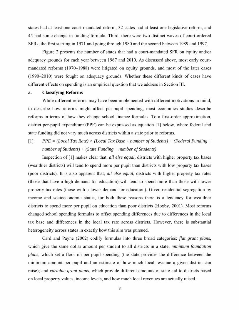
a. Classifying Reforms

While different reforms may have been implemented with different motivations in mind,

to describe how reforms might affect per-pupil spending, most economics studies describe

reforms in terms of how they change school finance formulas. To a first-order approximation,

district per-pupil expenditure (PPE) can be expressed as equation [1] below, where federal and

state funding did not vary much across districts within a state prior to reforms.

[1] PPE = (Local Tax Rate) × (Local Tax Base ÷ number of Students) + (Federal Funding ÷

number of Students) + (State Funding ÷ number of Students)

Inspection of [1] makes clear that, all else equal, districts with higher property tax bases

(wealthier districts) will tend to spend more per pupil than districts with low property tax bases

(poor districts). It is also apparent that, all else equal, districts with higher property tax rates

(those that have a high demand for education) will tend to spend more than those with lower

property tax rates (those with a lower demand for education). Given residential segregation by

income and socioeconomic status, for both these reasons there is a tendency for wealthier

districts to spend more per pupil on education than poor districts (Hoxby, 2001). Most reforms

changed school spending formulas to offset spending differences due to differences in the local

tax base and differences in the local tax rate across districts. However, there is substantial

heterogeneity across states in exactly how this aim was pursued.

Card and Payne (2002) codify formulas into three broad categories: flat grant plans,

which give the same dollar amount per student to all districts in a state; minimum foundation

plans, which set a floor on per-pupil spending (the state provides the difference between the

minimum amount per pupil and an estimate of how much local revenue a given district can

raise); and variable grant plans, which provide different amounts of state aid to districts based

on local property values, income levels, and how much local revenues are actually raised.

 

9  

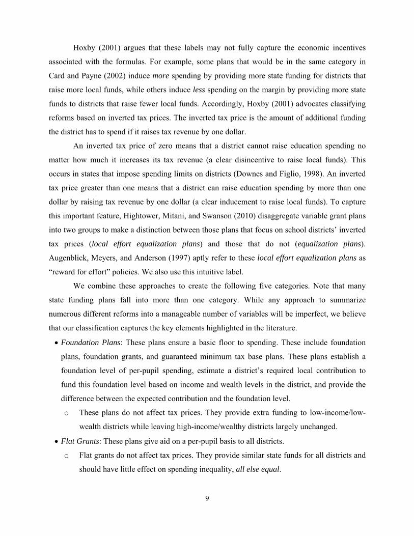
Hoxby (2001) argues that these labels may not fully capture the economic incentives

associated with the formulas. For example, some plans that would be in the same category in

Card and Payne (2002) induce more spending by providing more state funding for districts that

raise more local funds, while others induce less spending on the margin by providing more state

funds to districts that raise fewer local funds. Accordingly, Hoxby (2001) advocates classifying

reforms based on inverted tax prices. The inverted tax price is the amount of additional funding

the district has to spend if it raises tax revenue by one dollar.

An inverted tax price of zero means that a district cannot raise education spending no

matter how much it increases its tax revenue (a clear disincentive to raise local funds). This

occurs in states that impose spending limits on districts (Downes and Figlio, 1998). An inverted

tax price greater than one means that a district can raise education spending by more than one

dollar by raising tax revenue by one dollar (a clear inducement to raise local funds). To capture

this important feature, Hightower, Mitani, and Swanson (2010) disaggregate variable grant plans

into two groups to make a distinction between those plans that focus on school districts’ inverted

tax prices (local effort equalization plans) and those that do not (equalization plans).

Augenblick, Meyers, and Anderson (1997) aptly refer to these local effort equalization plans as

“reward for effort” policies. We also use this intuitive label.

We combine these approaches to create the following five categories. Note that many

state funding plans fall into more than one category. While any approach to summarize

numerous different reforms into a manageable number of variables will be imperfect, we believe

that our classification captures the key elements highlighted in the literature.

Foundation Plans: These plans ensure a basic floor to spending. These include foundation

plans, foundation grants, and guaranteed minimum tax base plans. These plans establish a

foundation level of per-pupil spending, estimate a district’s required local contribution to

fund this foundation level based on income and wealth levels in the district, and provide the

difference between the expected contribution and the foundation level.

o These plans do not affect tax prices. They provide extra funding to low-income/low-

wealth districts while leaving high-income/wealthy districts largely unchanged.

Flat Grants: These plans give aid on a per-pupil basis to all districts.

o Flat grants do not affect tax prices. They provide similar state funds for all districts and

should have little effect on spending inequality, all else equal.

 

10  

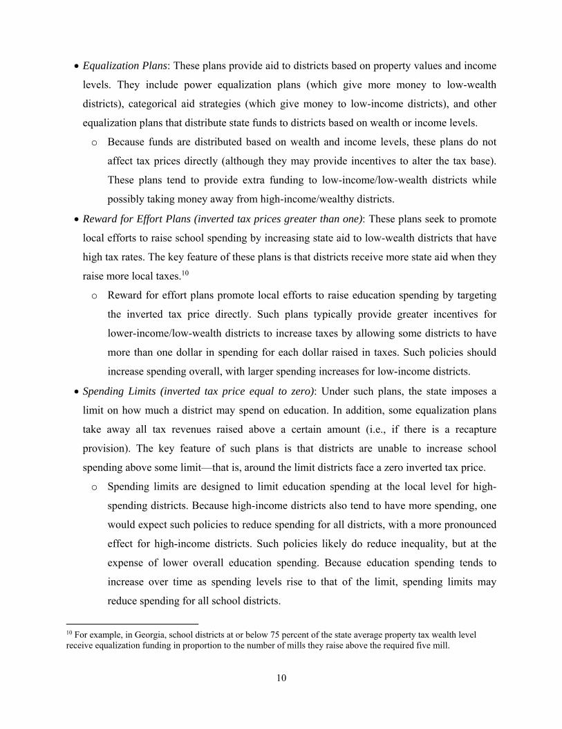
Equalization Plans: These plans provide aid to districts based on property values and income

levels. They include power equalization plans (which give more money to low-wealth

districts), categorical aid strategies (which give money to low-income districts), and other

equalization plans that distribute state funds to districts based on wealth or income levels.

o Because funds are distributed based on wealth and income levels, these plans do not

affect tax prices directly (although they may provide incentives to alter the tax base).

These plans tend to provide extra funding to low-income/low-wealth districts while

possibly taking money away from high-income/wealthy districts.

Reward for Effort Plans (inverted tax prices greater than one): These plans seek to promote

local efforts to raise school spending by increasing state aid to low-wealth districts that have

high tax rates. The key feature of these plans is that districts receive more state aid when they

raise more local taxes.10

o Reward for effort plans promote local efforts to raise education spending by targeting

the inverted tax price directly. Such plans typically provide greater incentives for

lower-income/low-wealth districts to increase taxes by allowing some districts to have

more than one dollar in spending for each dollar raised in taxes. Such policies should

increase spending overall, with larger spending increases for low-income districts.

Spending Limits (inverted tax price equal to zero): Under such plans, the state imposes a

limit on how much a district may spend on education. In addition, some equalization plans

take away all tax revenues raised above a certain amount (i.e., if there is a recapture

provision). The key feature of such plans is that districts are unable to increase school

spending above some limit—that is, around the limit districts face a zero inverted tax price.

o Spending limits are designed to limit education spending at the local level for high-

spending districts. Because high-income districts also tend to have more spending, one

would expect such policies to reduce spending for all districts, with a more pronounced

effect for high-income districts. Such policies likely do reduce inequality, but at the

expense of lower overall education spending. Because education spending tends to

increase over time as spending levels rise to that of the limit, spending limits may

reduce spending for all school districts.

                                                            10 For example, in Georgia, school districts at or below 75 percent of the state average property tax wealth level receive equalization funding in proportion to the number of mills they raise above the required five mill.

 

11  

b. Changes in School Finance Formulae Over Time

Since 1970, virtually every state has enacted at least one aid formula from among the

categories listed above. To provide an overview of the evolution of school finance formulas,

Figure 3 plots the number of states that have employed each kind of funding formula in each

year. The first notable pattern is that the use of foundation plans was quite high in 1970 and

increased slightly during the entire period (from 27 states in 1970 to 36 states in 2010). As more

states implemented SFRs, the use of flat grants declined (from 26 states in 1970 to 5 states in

2020), while the use of equalizing plans increased (from 9 states in 1970 to 30 states in 2010).

The reward for effort approach was unpopular in 1970, but the number of states employing

reward for effort has increased over time (from 0 states in 1970 to 21 states in 2010), as has the

number of states imposing spending limits (from 0 states in 1970 to 12 states in 2010). In Section

III we investigate the effects of these different kinds of reforms on the level and distribution of

school spending.

c. Changes in School Spending Over Time

Data on district and state funding come from the Census of Governments, the Historical

Database on Individual Government Finances (INDFIN),11 and the Common Core of Data

(CCD) School District Finance Survey (F-33). The Census of Governments has been conducted

every five years since 1967 and records administrative data on school spending for every school

district in the United States. This is the data source used in most existing national studies of

school finance reforms. We augment this data with annual data from other sources. The INDFIN

contains school district finance data annually for a sub-sample of large school districts from 1967

through 1991.12 After 1992, the CCD School District Finance Survey (F-33) consists of data

submitted annually to the National Center for Education Statistics (NCES) and includes data on

school spending for every school district in the United States.13 We combine these data sources

                                                            11 The Historical Database on Individual Government Finances (INDFIN) represents the Census Bureau’s first effort to provide a time series of historically consistent data on the finances of individual governments. This database combines data from the Census of Governments Survey of Government Finances (F-33), the National Archives, and the Individual Government Finances Survey. 12 Per-pupil spending data from before 1992 is missing for Alaska, Hawaii, Maryland, North Carolina, Virginia, and Washington, D.C. Per-pupil spending data from 1968 and 1969 is missing for all states. Spending data for certain years is also missing for the following states: Florida (1975, 1983, 1985–1987, and 1991); Kansas (1977 and 1986); Mississippi (1985 and 1988); Montana (1976); Nebraska (1977); Texas (1991); and Wyoming (1979 and 1984). Where data for only a year or two was missing, it was filled in using linear interpolation. 13 Both NCES and the Governments Division of the U.S. Census Bureau collect public school system finance data, and they collaborate in their efforts to gather these data. 

 

12  

to construct a long panel of annual per-pupil spending for school districts in the United States

between 1967 and 2010.

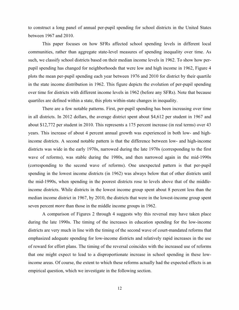
This paper focuses on how SFRs affected school spending levels in different local

communities, rather than aggregate state-level measures of spending inequality over time. As

such, we classify school districts based on their median income levels in 1962. To show how per-

pupil spending has changed for neighborhoods that were low and high income in 1962, Figure 4

plots the mean per-pupil spending each year between 1976 and 2010 for district by their quartile

in the state income distribution in 1962. This figure depicts the evolution of per-pupil spending

over time for districts with different income levels in 1962 (before any SFRs). Note that because

quartiles are defined within a state, this plots within-state changes in inequality.

There are a few notable patterns. First, per-pupil spending has been increasing over time

in all districts. In 2012 dollars, the average district spent about $4,612 per student in 1967 and

about $12,772 per student in 2010. This represents a 175 percent increase (in real terms) over 43

years. This increase of about 4 percent annual growth was experienced in both low- and high-

income districts. A second notable pattern is that the difference between low- and high-income

districts was wide in the early 1970s, narrowed during the late 1970s (corresponding to the first

wave of reforms), was stable during the 1980s, and then narrowed again in the mid-1990s

(corresponding to the second wave of reforms). One unexpected pattern is that per-pupil

spending in the lowest income districts (in 1962) was always below that of other districts until

the mid-1990s, when spending in the poorest districts rose to levels above that of the middle-

income districts. While districts in the lowest income group spent about 8 percent less than the

median income district in 1967, by 2010, the districts that were in the lowest-income group spent

seven percent more than those in the middle income groups in 1962.

A comparison of Figures 2 through 4 suggests why this reversal may have taken place

during the late 1990s. The timing of the increases in education spending for the low-income

districts are very much in line with the timing of the second wave of court-mandated reforms that

emphasized adequate spending for low-income districts and relatively rapid increases in the use

of reward for effort plans. The timing of the reversal coincides with the increased use of reforms

that one might expect to lead to a disproportionate increase in school spending in these low-

income areas. Of course, the extent to which these reforms actually had the expected effects is an

empirical question, which we investigate in the following section.

 

13  

III. Event-Study Analysis of Effects on School Spending

Our empirical approach to estimating the effect of SFR on the distribution of per-pupil

spending across district income levels is to analyze data using a Difference-in-Differences (DiD)

methodology. Using the district-by-year data as described in Section II, we can compare the

spending in low- or high-income districts (districts with low or high median incomes in 1962)

before implementation of a SFR to the spending in the same district after implementation.

Because there may be a tendency for spending to increase over time, we use the difference in

spending for low- or high-income districts across the same years in states that did not implement

any reforms over that time period as a basis for comparison.

To give an example, Illinois implemented its first SFR in 1973, while Missouri

implemented its first SFR in 1977. One can compare spending for low-income districts in Illinois

in 1972 (the year before the reform) to that in 1976 (four years post-reform). Because there may

have been some national and region-specific changes that affected spending in all districts

between 1972 and 1976, one can use the difference in spending for low-income districts between

1972 and 1976 in Missouri (both pre-reform years in MO) as an estimate of what the change in

spending would have been for low-income districts in Illinois absent reforms. If reforms increase

spending for low-income districts, we should see that the difference in spending for low-income

districts between 1972 and 1976 in Illinois is greater than the difference in spending for low-

income districts between 1972 and 1976 in Missouri. The same logic can be applied to spending

in medium- and high-income districts. This is the logic of the DiD estimator. One can implement

this DiD strategy within a regression framework by estimating equation [2], below.

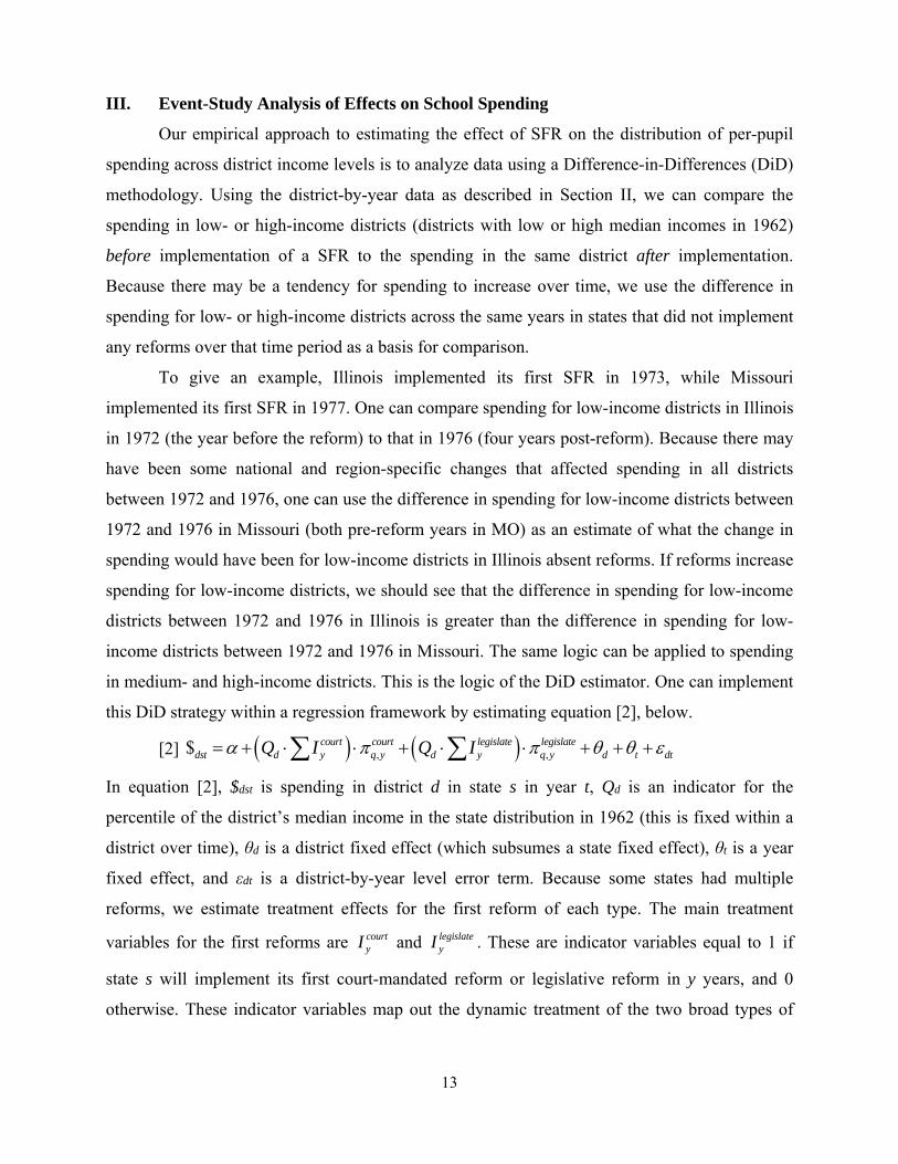
[2] , ,$ court court legislate legislatedst d y q y d y q y d t dtQ I Q I

In equation [2], $dst is spending in district d in state s in year t, Qd is an indicator for the

percentile of the district’s median income in the state distribution in 1962 (this is fixed within a

district over time), θd is a district fixed effect (which subsumes a state fixed effect), θt is a year

fixed effect, and εdt is a district-by-year level error term. Because some states had multiple

reforms, we estimate treatment effects for the first reform of each type. The main treatment

variables for the first reforms are courtyI  and  legislate

yI . These are indicator variables equal to 1 if

state s will implement its first court-mandated reform or legislative reform in y years, and 0

otherwise. These indicator variables map out the dynamic treatment of the two broad types of

 

14  

reforms and are interacted with Qd. The coefficients ,courtq y  map out the dynamic treatment effect

of the first court-mandated reform on per-pupil spending for districts in quartile q. Similarly, the

coefficients ,legislateq y  map out the dynamic treatment effect of the first legislative reform on per-

pupil spending for districts in quartile q. For example, 1, 10legislate is the effect today in a bottom

income quartile district of implementing the first legislative reform 10 years in the future, and

1,5legislate is the effect today in a bottom quartile district of having implemented the first legislative

reform in the bottom quartile five years ago. We plot the estimated treatment effects to illustrate

how per-pupil spending evolves in the years before, during, and after the first legislative and

court-mandated reforms. A visual inspection of this event-study plot should reveal any pre-

reform trends in spending and any structural break in outcomes.

Because different kinds of reforms may have different effects, we also estimate dynamic

treatment effects for different aspects of each reform by coding the first year that a district uses a

formula with a (a) spending limit, (b) local equalization, (c) foundation plan, or (d) equalization

plan. To estimate the dynamic treatment effect for particular types of funding formulae, we can

use equation [2] while replacing the reform-type indicators with limityI , localeq

yI , foundationyI , and

equalizationyI . These are indicator variables equal to 1 if state s will implement its first spending

limit, local equalization, foundation plan, or equalization plan in y years, and 0 otherwise. One

can then plot the coefficients on these indicators interacted with the district quartile to observe

how district per-pupil spending evolved before, during, and after the changing of the school

finance formulas in these specific ways.

To quantify the effect of these reforms on per-pupil spending, we form linear

combinations of the estimated treatment effects for different years. For example, the effect of

court-ordered reforms on the spending for the bottom 10 percent of income districts can be

estimated by the average of the 5 years after reforms minus the average of the 5 years prior to

reforms. This estimate is obtained by computing the following linear combination of coefficient

estimates: , 5 , 4 , 3 , 2 , 1 ,5 ,4 ,3 ,2 ,1( ) / 5 ( ) / 5court court court court court court court court court courtq q q q q q q q q q .

Whether this computed difference is statistically significant is determined by testing the

statistical significance of the linear combination of the estimated coefficients. We present the

results of such tests to accompany the event-study graphs. Note that the standard errors for all the

 

15  

estimates are clustered at the state level.

a. Event-Study Analysis for Court-Mandated Reforms

Much of the empirical literature of SFR has focused on court-mandated reforms. Figure 5

presents the event-study graph for court-mandated reforms for school districts in different

percentiles of the income distribution in 1962 (a year before any reforms were implemented).

The figure depicts how district-level per-pupil spending evolved annually from nine years prior

to the first court-mandated reforms through 20 years after the reforms. The evolution of spending

is presented separately for districts in the bottom 10 percent of median incomes, those in the 11th

to 25th percentile, those in the 26th to 50th percentile, those in the 51th to 75th percentile, those in

the 76th to 90th percentile, and those in the top 10 percent. The series for the bottom 10 percent

depicts how per-pupil spending evolved for districts in the bottom 10 percent of the state income

distribution over time in states with a court-mandated reform, relative to such districts in states

without a court-mandated reform over the same time period. To show how per-pupil spending

was affected for all districts on the same scale, each series is re-centered around the average for

the 10 years prior to reforms. This means that a value of 0 in a given year would indicate that

spending in that year was the same as the 10-year average prior to reforms. Also, note that year 0

is the year of the reform. As such, if reforms increase spending relative to pre-reform years, we

should see positive values for years 1 through 20, and if reforms decrease spending, we should

see negative values for these years.

In Figure 5, all the series are centered on 0 during the pre-reform years. During the 10

years prior to reforms (years -10 through -1), districts in reform states saw similar changes in

per-pupil spending as districts in non-reform states of the same income level. Within the first five

post-reform years however, districts in the bottom quartile (solid black lines) saw increases in

per-pupil spending above and beyond comparison districts in non-reform states. Districts

between the 25th and 75th percentiles experienced modest increases after reforms (as evidenced

by most post-reform data points for these districts being above the pre-reform mean). In contrast,

districts in the top 25 percent of incomes in 1962 saw little change in spending within the first 14

years after reforms, and there is evidence of a slight decrease 15 years after reforms for the very

highest income districts. Note that the sharp decline in spending at year 8 is due to a

compositional change. The lower panel of Figure 5 plots the same dynamic treatment effects, but

only using districts that were observed for more than 10 post-reform years. Using this more

balanced panel, there is no sudden drop in year 9, but the basic patterns are similar (increased

 

16  

school spending for the lowest-income districts and decreases for the highest-spending districts).

Because the more balanced panel includes only older cases, it includes relatively few adequacy

cases. We will show that the difference between the top and bottom panels of Figure 5 is due to

the fact that the first seven years presented in the top panel include many recent adequacy cases,

and these generate somewhat different patterns from the older equity cases.

To better quantify the patterns in Figure 5, we estimate the effect of court-mandated

reform as the difference between the average effect in the 10 years prior to reforms and the 10

years after reforms. Based on the linear combination of coefficient estimates, these reforms

increased per-pupil spending for the bottom 10 percent income districts over the first 10 years by

$582.81 in 2010 dollars (p-value=0.07). Between 1980 and 1990, the average per-pupil spending

for these low-income districts was $6,590.66, representing a relative spending increase of about

nine percent. To get a better sense of the longer run effects of spending for these districts, we

compute the average effect for years 5 through 10 relative to the 10 years prior to reforms. This

calculation indicates that after five years these reforms increased per-pupil spending for the

bottom 10 percent income districts by $651.12 (p-value=0.02), an increase in spending for low-

income districts of about 11 percent. Similar calculations for the top 10 percent income districts

show little effect. The estimated effects suggest that these reforms reduced spending during the

first 10 years by $110.41 (p-value=0.27) and in years 5 through 10 by $191.12 (p-value=0.56).

In sum, court-mandated reforms increased spending in the lowest-income districts by

about 10 percent and had little effect for the highest-income districts. Using the estimates, after

10 years court-mandated reforms reduced the spending gap between the top-income districts and

the bottom-income districts by $842.01 (p-value<0.01). The spending gap between these two

groups of districts between 1980 and 1990 was $1,197.33, so that court-mandated reforms

reduced this spending gap by about 70 percent on average. The magnitude of these effects,

coupled with the rapid increase in the number of court-mandated reforms during the early 1990s,

can account for a sizable portion of the spending “catch-up” documented in Figure 4 between the

lowest- and highest-income districts.

There are two types of court-mandated reforms: those argued on equity grounds and

those argued on adequacy grounds. One might wonder if these different kinds of cases lead to

different kinds of reforms that have different effects. This question was investigated empirically

by Springer, Liu, and Guthrie (2009) and Berry (2007), who found no difference between these

two kinds of cases in simple regression settings. We investigate this question using the more

 

17  

flexible event-study approach.

The top panel of Figure 6 presents the dynamic effects of equity-based court-mandated

reforms on the level of per-pupil spending. The effects are relative to non-reform states. There is

a dip in spending (of about $500) in all districts two years prior to reforms for those states that

had their first court-mandated case based on equity grounds relative to similarly affluent districts

in non-reform states. While this pre-reform dip makes the effect of such cases on the overall

level of spending unclear (because it is unclear what the trajectory of school spending would

have looked like absent reforms), it is apparent that equity cases do lead to greater equity in

spending: while the top-income and bottom-income districts are on very similar trajectories prior

to reforms, such that the spending gap was stable in the pre-treatment years, the spending gap

narrowed by $807.54 (p-value=0.01) after five years post-reform. The aim of these cases was to

increase spending equity. Reforms induced by these equity based cases achieved this objective.

The bottom panel of Figure 6 presents the event-study graph for adequacy cases

(primarily the second wave of cases). The objective of these cases was not to explicitly reduce

inequality in education spending, but rather to ensure that spending permitted all children

(especially those in low-income districts) to receive adequate resources for a quality education.

Because these cases are more recent, we present the dynamic treatment for the first seven years

of the reform. As one can see, spending in all districts in states with adequacy cases was fairly

stable (relative to non-reform districts) prior to reforms. The trajectory of spending was quite flat

four years prior to reforms. After reforms, there is evidence of an increase in school spending

that is most pronounced for the poorest 10 percent of districts. While all districts experience an

increase in spending of about $430 within the first five years of reforms, the poorest 10 percent

of districts break from the other districts with an increase in spending of over $1,000 within the

first five years. Because all districts experienced spending increases, adequacy cases are

associated with a smaller reduction in spending gaps than equity cases. Five years after an

adequacy case, the gap in spending between the highest- and lowest-income districts is narrowed

by $377.25 (p-value=0.02). In sum, consistent with the aims articulated by the courts, equity

cases led to greater equity in school spending, while adequacy cases led to increased school

spending overall, with particularly large increases for low-income districts.

b. Event-Study Analysis for Legislative Reforms

Legislative reforms have received much less attention in the literature than court-

mandated reforms, and the consensus seems to be that legislative reforms were largely

 

18  

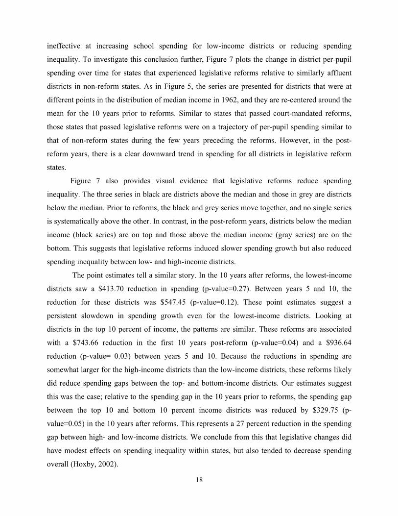
ineffective at increasing school spending for low-income districts or reducing spending

inequality. To investigate this conclusion further, Figure 7 plots the change in district per-pupil

spending over time for states that experienced legislative reforms relative to similarly affluent

districts in non-reform states. As in Figure 5, the series are presented for districts that were at

different points in the distribution of median income in 1962, and they are re-centered around the

mean for the 10 years prior to reforms. Similar to states that passed court-mandated reforms,

those states that passed legislative reforms were on a trajectory of per-pupil spending similar to

that of non-reform states during the few years preceding the reforms. However, in the post-

reform years, there is a clear downward trend in spending for all districts in legislative reform

states.

Figure 7 also provides visual evidence that legislative reforms reduce spending

inequality. The three series in black are districts above the median and those in grey are districts

below the median. Prior to reforms, the black and grey series move together, and no single series

is systematically above the other. In contrast, in the post-reform years, districts below the median

income (black series) are on top and those above the median income (gray series) are on the

bottom. This suggests that legislative reforms induced slower spending growth but also reduced

spending inequality between low- and high-income districts.

The point estimates tell a similar story. In the 10 years after reforms, the lowest-income

districts saw a $413.70 reduction in spending (p-value=0.27). Between years 5 and 10, the

reduction for these districts was $547.45 (p-value=0.12). These point estimates suggest a

persistent slowdown in spending growth even for the lowest-income districts. Looking at

districts in the top 10 percent of income, the patterns are similar. These reforms are associated

with a $743.66 reduction in the first 10 years post-reform (p-value=0.04) and a $936.64

reduction (p-value= 0.03) between years 5 and 10. Because the reductions in spending are

somewhat larger for the high-income districts than the low-income districts, these reforms likely

did reduce spending gaps between the top- and bottom-income districts. Our estimates suggest

this was the case; relative to the spending gap in the 10 years prior to reforms, the spending gap

between the top 10 and bottom 10 percent income districts was reduced by $329.75 (p-

value=0.05) in the 10 years after reforms. This represents a 27 percent reduction in the spending

gap between high- and low-income districts. We conclude from this that legislative changes did

have modest effects on spending inequality within states, but also tended to decrease spending

overall (Hoxby, 2002).

 

19  

c. Effects by Type of Reform Used

While documenting the effects of past court ordered and legislative reforms is important

from an historical point of view, it does not address the policy-relevant question of why different

kinds of reforms have different effects or what kinds of reforms policy-makers should try to

implement in the future. There are numerous ways that reforms can be constructed, and it can be

argued that what really matters is the kind of funding formula used in a reform, rather than why

or how the reform was implemented. Furthermore, as illustrated in Figure 1, there are many more

funding changes that may affect the distribution of school spending that are not tied to specific

legislative or court-mandated reforms. This motivates an event-study analysis of the four most

commonly introduced types of reforms. Because flat grants were not introduced over time, but

rather replaced with new reforms, we do not estimate the effects of introducing flat grants.

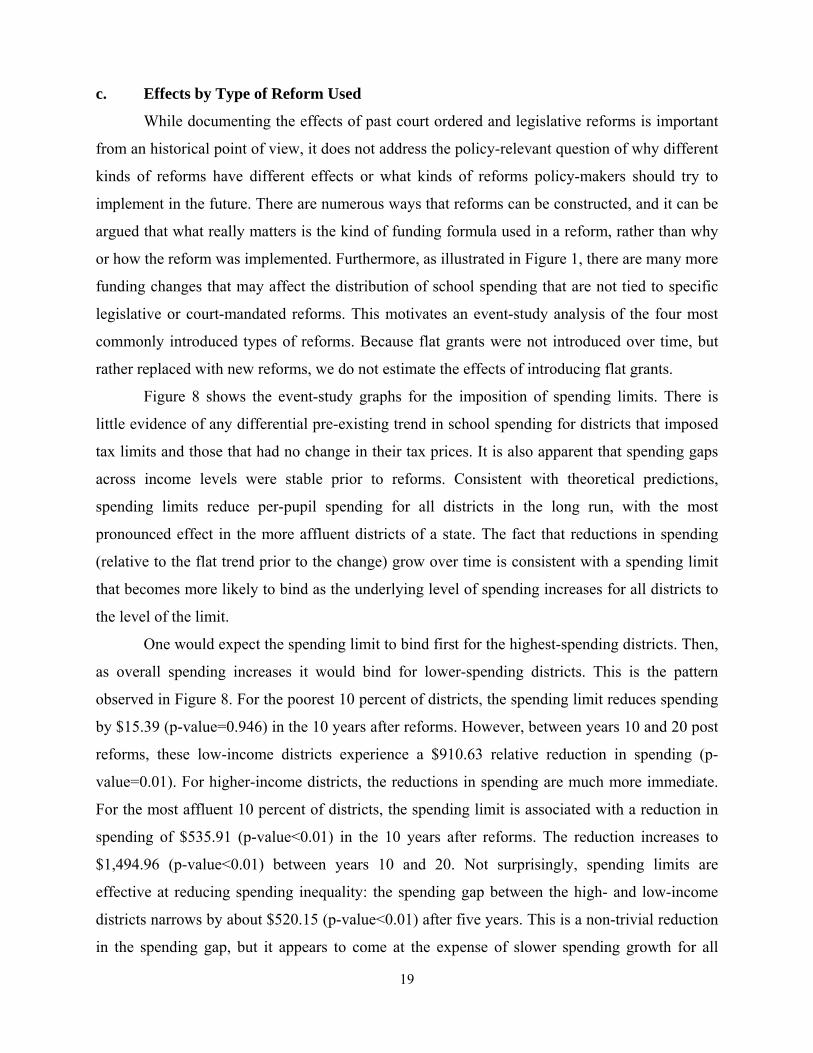
Figure 8 shows the event-study graphs for the imposition of spending limits. There is

little evidence of any differential pre-existing trend in school spending for districts that imposed

tax limits and those that had no change in their tax prices. It is also apparent that spending gaps

across income levels were stable prior to reforms. Consistent with theoretical predictions,

spending limits reduce per-pupil spending for all districts in the long run, with the most

pronounced effect in the more affluent districts of a state. The fact that reductions in spending

(relative to the flat trend prior to the change) grow over time is consistent with a spending limit

that becomes more likely to bind as the underlying level of spending increases for all districts to

the level of the limit.

One would expect the spending limit to bind first for the highest-spending districts. Then,

as overall spending increases it would bind for lower-spending districts. This is the pattern

observed in Figure 8. For the poorest 10 percent of districts, the spending limit reduces spending

by $15.39 (p-value=0.946) in the 10 years after reforms. However, between years 10 and 20 post

reforms, these low-income districts experience a $910.63 relative reduction in spending (p-

value=0.01). For higher-income districts, the reductions in spending are much more immediate.

For the most affluent 10 percent of districts, the spending limit is associated with a reduction in

spending of $535.91 (p-value<0.01) in the 10 years after reforms. The reduction increases to

$1,494.96 (p-value<0.01) between years 10 and 20. Not surprisingly, spending limits are

effective at reducing spending inequality: the spending gap between the high- and low-income

districts narrows by about $520.15 (p-value<0.01) after five years. This is a non-trivial reduction

in the spending gap, but it appears to come at the expense of slower spending growth for all

 

20  

districts. The decreases in spending are consistent with the theoretical prediction that decreases

in inverted tax prices will tend to decrease the overall level of school spending.

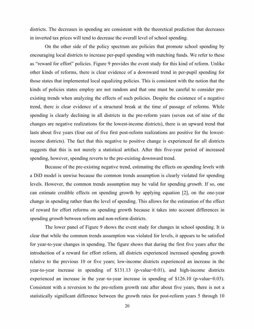
On the other side of the policy spectrum are policies that promote school spending by

encouraging local districts to increase per-pupil spending with matching funds. We refer to these

as “reward for effort” policies. Figure 9 provides the event study for this kind of reform. Unlike

other kinds of reforms, there is clear evidence of a downward trend in per-pupil spending for

those states that implemented local equalizing policies. This is consistent with the notion that the

kinds of policies states employ are not random and that one must be careful to consider pre-

existing trends when analyzing the effects of such policies. Despite the existence of a negative

trend, there is clear evidence of a structural break at the time of passage of reforms. While

spending is clearly declining in all districts in the pre-reform years (seven out of nine of the

changes are negative realizations for the lowest-income districts), there is an upward trend that

lasts about five years (four out of five first post-reform realizations are positive for the lowest-

income districts). The fact that this negative to positive change is experienced for all districts

suggests that this is not merely a statistical artifact. After this five-year period of increased

spending, however, spending reverts to the pre-existing downward trend.

Because of the pre-existing negative trend, estimating the effects on spending levels with

a DiD model is unwise because the common trends assumption is clearly violated for spending

levels. However, the common trends assumption may be valid for spending growth. If so, one

can estimate credible effects on spending growth by applying equation [2], on the one-year

change in spending rather than the level of spending. This allows for the estimation of the effect

of reward for effort reforms on spending growth because it takes into account differences in

spending growth between reform and non-reform districts.

The lower panel of Figure 9 shows the event study for changes in school spending. It is

clear that while the common trends assumption was violated for levels, it appears to be satisfied

for year-to-year changes in spending. The figure shows that during the first five years after the

introduction of a reward for effort reform, all districts experienced increased spending growth

relative to the previous 10 or five years; low-income districts experienced an increase in the

year-to-year increase in spending of $131.13 (p-value=0.01), and high-income districts

experienced an increase in the year–to-year increase in spending of $126.10 (p-value=0.03).

Consistent with a reversion to the pre-reform growth rate after about five years, there is not a

statistically significant difference between the growth rates for post-reform years 5 through 10

 

21  

and the pre-reform years (i.e., both yield p-values above 0.1). However, there is evidence

suggestive of increased spending growth for the lowest-income districts in the long run such that

during post-reform years 10 through 20, average annual spending changes were $175.88 more

(p-value=0.08) than during the pre-reform years. This is consistent with the analysis in levels that

reveals that reward-for-effort plans reduce the spending gap between low- and high-income

districts in the long run by $295.83 (p-value=0.11). Overall, the patterns show an increase in

spending and spending growth in the short run (lasting about five years after reforms) for all

districts, with a possible permanent increase in spending growth for the poorest districts. Results

suggest that these policies increase the growth of spending (particularly for low-income districts)

and reduce spending gaps between high- and low-income districts by about 12 percent.

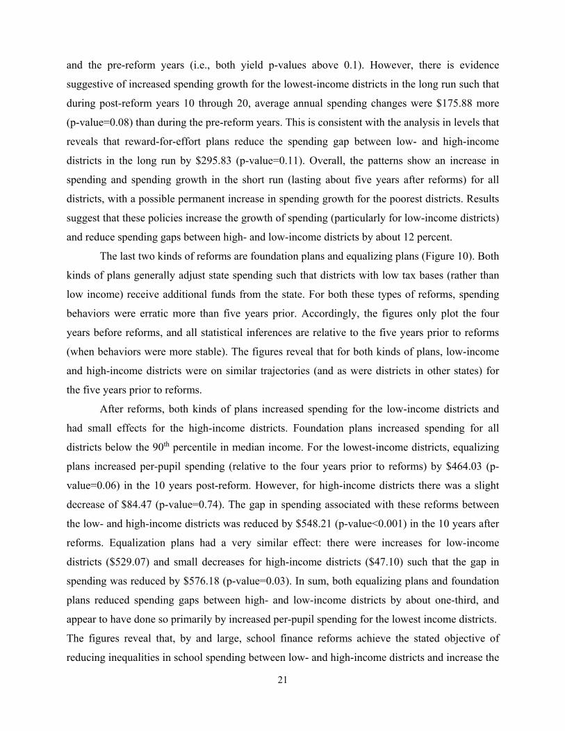
The last two kinds of reforms are foundation plans and equalizing plans (Figure 10). Both

kinds of plans generally adjust state spending such that districts with low tax bases (rather than

low income) receive additional funds from the state. For both these types of reforms, spending

behaviors were erratic more than five years prior. Accordingly, the figures only plot the four

years before reforms, and all statistical inferences are relative to the five years prior to reforms

(when behaviors were more stable). The figures reveal that for both kinds of plans, low-income

and high-income districts were on similar trajectories (and as were districts in other states) for

the five years prior to reforms.

After reforms, both kinds of plans increased spending for the low-income districts and

had small effects for the high-income districts. Foundation plans increased spending for all

districts below the 90th percentile in median income. For the lowest-income districts, equalizing

plans increased per-pupil spending (relative to the four years prior to reforms) by $464.03 (p-

value=0.06) in the 10 years post-reform. However, for high-income districts there was a slight

decrease of $84.47 (p-value=0.74). The gap in spending associated with these reforms between

the low- and high-income districts was reduced by $548.21 (p-value<0.001) in the 10 years after

reforms. Equalization plans had a very similar effect: there were increases for low-income

districts ($529.07) and small decreases for high-income districts ($47.10) such that the gap in

spending was reduced by $576.18 (p-value=0.03). In sum, both equalizing plans and foundation

plans reduced spending gaps between high- and low-income districts by about one-third, and

appear to have done so primarily by increased per-pupil spending for the lowest income districts.

The figures reveal that, by and large, school finance reforms achieve the stated objective of

reducing inequalities in school spending between low- and high-income districts and increase the

 

22  

level of per-pupil spending in poor communities. Both equalization plans and foundation plans

are effective at reducing spending gaps between low- and high-income areas. The results also

indicate that plans that aim to increase equality by reducing spending for the highest-income

districts achieve this objective, but with the unintended impact of also reducing spending in low-

income districts in the long run. In contrast, plans that promote greater education spending

through matching tend to have a positive effect on the growth of school spending for all districts,

with particularly large effects for low-income districts. Having established to what extent and

how SFRs change the distribution of school spending, the remaining question is how changes in

school spending caused by these reforms affect the educational and adult economic outcomes of

children. This is the topic of Part Two.

PART TWO: EFFECTS OF SCHOOL SPENDING ON LONG-RUN OUTCOMES

IV. Description of the Longer-Run Outcome Data

The primary micro dataset utilized to analyze the effects of reform-induced changes in

school spending on long-run outcomes is the restricted, confidential geocoded version of the

PSID (1968–2011) with identifiers at the level of the neighborhood blocks in which children

grew up.14 We link our district-level data on school spending and the timing of reforms to the

nationally-representative sample of children born between 1955 and 1985 from the PSID.

Following Johnson (2012), we then merge neighborhood and school characteristics, as well as

information on other key policy changes (e.g., the timing of school desegregation, hospital

desegregation, rollout of “War on Poverty” initiatives, and expansion of safety net programs)

from multiple data sources on the conditions that prevailed when these children were growing

up, allowing for a rich set of control variables.15

                                                            14 The PSID began interviewing a national probability sample of families in 1968. These families were re-interviewed each year through 1997, when interviewing became biennial. All persons in PSID families in 1968 have the PSID “gene,” which means that they are followed in subsequent waves. When children with the “gene” become adults and leave their parents’ homes, they become their own PSID “family unit” and are interviewed in each wave. The original geographic cluster design of the PSID enables comparisons in adulthood of childhood neighbors who have been followed over the life course. 15 The data we use include measures from 1968–1988 Office of Civil Rights (OCR) data; 1960, 1970, 1980, and 1990 Census data; 1962–1999 Census of Governments (COG) data; Common Core Data (CCD) compiled by the National Center for Education Statistics; Regional Economic Information System (REIS) data; a comprehensive case inventory of court litigation regarding school desegregation over the 1955–1990 period (American Communities Project); and the American Hospital Association’s Annual Survey of Hospitals (1946–1990) and the  

 

23  

The sample consists of PSID sample members born between 1955 and 1985 who have

been followed into adulthood; these individuals were between the ages of 26 and 56 in 2011. We

include all information on them for each wave, 1968 to 2011.16 We include both the Survey

Research Center (SRC) component and the Survey of Economic Opportunity (SEO) component,

commonly known as the “poverty sample,” of the PSID sample. Due to the oversampling of

African-American and low-income families, 59 percent of the sample members were poor as

children (N=15,353 individuals; 9,035 poor children; 6,318 non-poor children). Sixty-six percent

of the PSID individuals born between 1955 and 1985 and followed into adulthood grew up in a

school district that was subject to a court-mandated school finance reform sometime between

1972 and 2000, with the timing of the court order not necessarily occurring during their school-

age years. Eighty-eight percent of the PSID individuals born between 1955 and 1985 who were

poor as children and followed into adulthood grew up in a school district that was subject to a

court-mandated school finance reform sometime between 1972 and 2000. Given the patterns in

Figure 1, the share of individuals exposed to school finance reforms during childhood increases

significantly with birth year over the 1955–1985 birth cohorts analyzed in the PSID sample.

We use the census block as the definition of neighborhood, which comprises a smaller

geographic area than most previous studies utilize, and we match childhood residential location

address histories to blocks and school district boundaries that prevailed in 1969 (the algorithm is

outlined in Appendix A).17 Each record is merged with data on school spending for 1960–2000

and the aforementioned school finance variables at the school district level that correspond with

the prevailing levels during their school-age years. We also merge information on student-

teacher ratios and school segregation indices to the PSID data using the census block/tract

contained in the geocode file based on the earliest available address in childhood (or county of

birth when census block information is unavailable).

After combining information from these data sources, the main sample used to analyze

adult attainment outcomes consists of PSID individuals born between 1955 and 1985. It includes

                                                                                                                                                                                                Centers for Medicare and Medicaid Services data files (dating back to the 1960s) to identify the precise date in which a Medicare-certified hospital was established in each county of the U.S. (an accurate marker for hospital desegregation compliance). 16 The PSID maintains high wave-to-wave response rates of 95–98 percent. Studies have concluded that the PSID sample of heads of households and spouses remains representative of the national sample of adults (Gottschalk et al., 1999; Becketti et al., 1997). 17 Many school districts were counties during this period, including more than one-half of Southern school districts.

 

24  

93,022 adult person-year observations of 15,353 individuals (9,035 poor children; 6,318 non-

poor children) from 1,409 school districts, 1,031 counties, and all 50 states and the District of

Columbia. Given the data structure, the oldest cohort is observed at age 56, while many cohorts

are observed at age 30. To compare individuals from different cohorts at around the same age,

we focus on those adult observations between the ages of 25 and 45. The mean age is 32.9 years

for the economic outcome measures considered. The set of adult outcomes examined

chronologically over the life cycle include (a) educational outcomes—whether graduated from

high school, years of completed education – and (b) labor market and economic status outcomes

(all expressed in 2000 dollars)—wages, family income, and annual incidence of poverty in

adulthood (ages 25–45). All analyses include men and women with controls for gender.

Summary statistics are presented in Table 1.

V. Empirical Strategy for Estimating Effects on Adult Outcomes

In this section, we investigate whether changes in school spending induced by SFRs have

long-run impacts on adult outcomes. Particular attention is given to determine whether the

increased school spending experienced by children in lower-income communities due to SFRs

had any lasting effects on their adult socioeconomic well-being. Our empirical approach uses

two distinct sources of variation in per-pupil spending experienced during one’s school-age

years: first we exploit the staggered timing of court-mandated school finance reforms across

districts to implement a cohort level “event-study” analysis (variation in the timing of reforms

across cohorts); second, we exploit the fact that the same reform led to different changes in

spending across districts (variation in treatment intensity for exposed cohorts). We detail how all

this variation is used within a single framework in Section V.b.

While Part I shows that many reforms change the distribution of school spending, we

focus the analysis in Part II on school spending changes associated with the passage of court-

ordered reforms. This choice was driven by the fact that court-mandated reforms exhibited

minimal trending in spending prior to those reforms (suggesting that there might be minimal pre-

reform trending in adult outcomes across cohorts), and court-mandated reforms generated large,

robust, and statistically significant increases in per-pupil spending for low-income

neighborhoods (within which many of the PSID respondents resided).

While understanding the effect of school finance reforms on adult outcomes is important,

exploiting exogenous variation in per-pupil spending due to reforms allows for an investigation

 

25  

into the broader question of whether increasing school spending can improve the longer run

outcomes of affected students. Simply comparing outcomes of students exposed to more or less

school spending, even within the same district, could lead to biased estimates of the effect of

school spending on student outcomes, if there were other factors that affect both student

outcomes and school spending simultaneously. For example, a decline in the local economy

could depress per-pupil spending (through home prices or tax rates) and also have deleterious

effects on student outcomes through mechanisms unrelated to school spending such as parental

income. This would result in a spurious positive correlation between per-pupil spending and

child outcomes. Conversely, an inflow of low-income students might lead to an inflow of

compensatory federal funding while simultaneously generating reduced student outcomes. This

would lead to a spurious negative relationship between spending and student outcomes.

By focusing only on exogenous changes in school spending within districts associated

with reforms, our approach removes potential biases that might exist when simply comparing

students who have been exposed to different levels of school spending for reasons unknown to

the researcher. As in the analysis of school spending, we employ a flexible event-study design to

map how adult outcomes evolve over time (i.e. across cohorts) before and after reform-induced

changes in school spending. The event-study models allow us to examine how subsequent adult

outcomes are impacted by both the amount of (reform-induced) changes in school spending as

well as the duration of exposure to these spending changes during one’s school-age years. The

design also allows us to examine pre-reform trends in outcomes to test for potential endogeneity

of the timing of reforms. In Section VI, we show that isolating exogenous variation in school

spending leads one to very different conclusions about the productivity of education spending

than simple comparisons that do not account for the possibility that changes in school spending

might be endogenous to student outcomes.

a. Hypothesized Effects Across Cohorts

There are two natural tests of whether spending changes associated with school finance

reforms have a causal effect on adult outcomes. The first test is whether exposed cohorts from

those districts that experienced increases in per-pupil school spending also had improved

outcomes relative to unexposed cohorts from the same district. The second test is whether the

improvements observed for exposed cohorts (relative to unexposed cohorts) are larger for those

from districts that experienced larger increases in per-pupil school spending. Because not all

cohorts within a district are equally treated (some are exposed to spending increases for more of

 

26  

their school years than others), and not all districts experience the same changes in spending after

reforms (some districts experience larger spending increases than others), both of these tests can

be implemented within a single event-study framework. We lay out the cross-cohort and cross-

district patterns in outcomes one should observe in an event-study analysis if there is a causal

effect of increased spending due to reforms on adult outcomes.

If there is a causal effect of increased school spending on adult outcomes, and there are

no pre-existing cohort trend differences across districts that experience increases in spending,

then an event-time figure across cohorts for a given increase in school spending should follow

patterns similar to the stylized patterns presented in Figure 11. On the x-axis is the years of

exposure to the reform for a given cohort, and on the y-axis is the cohort-level mean of some

outcome for which higher values are better.

For those cohorts who were too old to be exposed to any reform-induced spending

increases (to the left of 0 such that they were 18 or older at the time of the passage of reforms),

there should be no systematic increase or decrease in the outcome across cohorts because none of

these cohorts was exposed. As such, an event-study graph of outcomes by cohort should be

relatively flat across cohorts that were too old to be affected by the reforms. Also, because pre-

reform cohorts are not exposed to any spending changes, outcomes should be similar across the

pre-reform cohorts both in districts that experienced large increases in school spending due to

reforms and those that experienced small increases in school spending due to reforms.

For those cohorts who were of school-going age when reforms were implemented (i.e.

those who were between the ages of 5 and 17, indicated by relative years 0 to 12 on the x-axis),

outcomes should both be better than those for the unexposed cohorts and increasing in the

number of years of exposure. That is, cohorts that are exposed to increased spending for a longer

period of time should have better outcomes than cohorts exposed to the same spending increase

but for a shorter period of time (variation in timing). Additionally, for a given duration of

exposure, individuals from districts that experienced larger increases in spending should have

larger improvements in outcomes than those from districts with smaller increases in spending

(variation in intensity). As such, the relationship between years of exposure and good outcomes

should be positive and it should be more positive for districts that experience larger increases in

spending. This is depicted in the two upward sloping segments for the partially exposed cohorts,

where the dashed line is steeper for larger increases in spending.

Finally, among more recent cohorts (i.e., those who were younger than 5 or unborn at the

 

27  

passage of reforms) all 12 of their school-age years were post-reform, and as a result, we

hypothesize these cohorts should have better outcomes than the partially exposed cohorts, and

there should be no systematic increase or decrease in the outcome among these fully treated

cohorts. As with the partially exposed cohorts, for a given duration of exposure individuals in

districts with larger increases in spending should have larger improvements in outcomes than

those in districts that experienced smaller increases in spending. This leads to better outcomes

(relative to untreated cohorts) for the fully treated cohorts from high-increase spending districts

than low-increase spending districts.

In sum, if (a) there is a causal effect of spending on outcomes and (b) the district-level

spending increases due to reforms are exogenous to changes in the outcomes, then the plot of the

event-time indicator variables for districts that experience small and large spending increases due

to reforms should follow the stylized patterns in Figure 11. That is, outcomes should be

improving in years of exposure to reforms (variation in time) and the relative improvements

should be larger in districts that experienced larger increases in school spending (variation in

intensity).

b. Analyzing the Effect of School Spending on Adult Outcomes

To show evidence of causal relationships, we test for the specific patterns hypothesized in

Figure 11 semi-parametrically across a variety of adult outcomes. While looking for differences

across cohorts can be achieved with a flexible event-study analysis, testing for differences across

districts that experienced larger or smaller increases in spending requires a good measure of the

court-mandated reform-induced increase in school spending. The event-study analysis

documented that districts in the bottom quartile of the state’s income distribution in 1962

experienced larger increases in school spending than those in high-income quartiles. As such, the

district’s quartile in the income distribution pre-reform could serve as a proxy for the extent to

which reforms increased funding in the district. However, this is a relatively weak proxy for

increases in spending at the individual district level because (a) not all court-mandated reforms

had the same effect on all districts, and (b) not all reforms had the same distributional effects on

districts within a state. As such, to test for whether those districts that experienced larger

increases in school spending were those that experienced larger improvements in adult outcomes

requires having a good measure of the increases in school spending resultant from the

implementation of a court-mandated reform at the individual district level.

To obtain a measure of district-specific changes in spending caused by court-mandated

 

28  

reforms, we regress the natural log of district per-pupil spending on district fixed effects, year

fixed effects, and an indicator variable denoting a post-reform year interacted with each school

district. To isolate spending changes associated with the court-ordered reforms, we also include

controls for a variety of potentially confounding policies. The period under study overlaps other

important policy changes (Johnson, 2013; Chay, Guryan, & Mazumder, 2009; Hoynes,

Schanzenbach, & Almond, 2012). To account for the effect of these policy changes, we include

county by year measures of school desegregation, hospital desegregation, community health

centers, and state funding for kindergarten, in addition to per capita expenditures on Head Start,

Title I school funding, and average childhood spending on food stamps, Aid to Families with

Dependent Children (AFDC), Medicaid, and unemployment insurance. 18 The coefficients on the

district indicators interacted with the post-reform indicator provide the regression estimate of the

change in per-pupil spending associated with the passage of a court-mandated reform for each

district (net of the effect of a myriad of other policies). For each district, we take the interaction

of the post-reform indicator with that district as our time-invariant, district-specific, court-

mandated reform effect on spending (“ cSPEND ”). Using this measure of treatment intensity (the

increase in per-pupil spending that the district will experience after the passage of reforms)

allows for a direct test of our key hypothesis—that exposed cohorts in those districts that

experienced larger increases in school spending also experienced greater improvements in

outcomes relative to unexposed cohorts in the same district.19

While we impose a monotonic relationship between increases in spending and the adult

outcomes with our parameterization of the treatment intensity variable, we remain flexible in our

estimation of the timing of effects across cohorts using an event-study design. The main event-

study models used to analyze the impacts of reform-induced changes in school spending on the

difference in adult attainment between treated and untreated cohorts involve estimating equations

of the form [3]:20

                                                            18 The data sources used to compile these measures are detailed in Johnson (2013). 19 Consistent with the flexible district-specific effects picking up much of the variability associated with the district income quartiles, it is much more positive for lower-income districts. However, one can only explain four percent of the variability across districts in

cSPEND with the district income quartile category variables. Using all the observable variables to describe reforms from Part One interacted with the quartile of income can predictably explain about one-third of the variability in

cSPEND . 20 This part of the research design is similar in setup to a recent study by Johnson (2011) on the long-run impacts of court-ordered school desegregation.

 

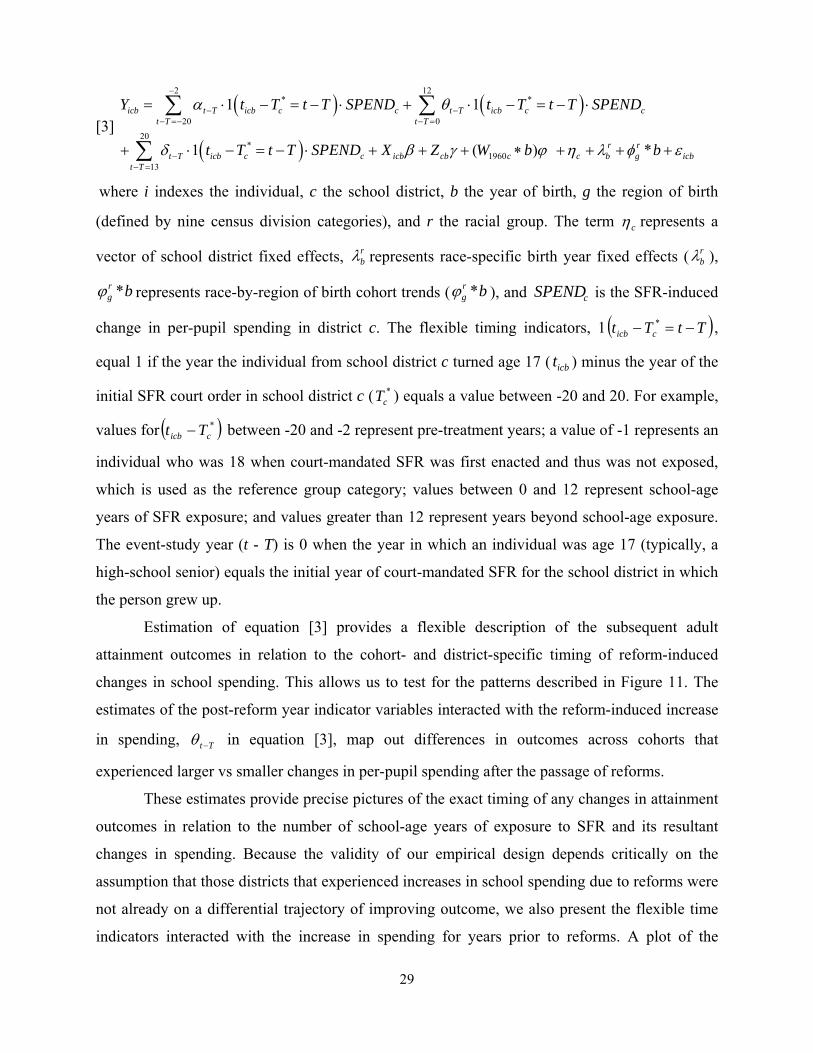
29  

[3]

2 12* *

20 020

*1960

13

1 1

1 ( ) *

icb t T icb c c t T icb c ct T t T

r rt T icb c c icb cb c c b g icb

t T

Y t T t T SPEND t T t T SPEND

t T t T SPEND X Z W b b

 where i indexes the individual, c the school district, b the year of birth, g the region of birth

(defined by nine census division categories), and r the racial group. The term c represents a

vector of school district fixed effects, represents race-specific birth year fixed effects ( ),

represents race-by-region of birth cohort trends ( ), and cSPEND is the SFR-induced

change in per-pupil spending in district c. The flexible timing indicators, 1 TtTt cicb * ,

equal 1 if the year the individual from school district c turned age 17 ( icbt ) minus the year of the

initial SFR court order in school district c ( *cT ) equals a value between -20 and 20. For example,

values for *cicb Tt between -20 and -2 represent pre-treatment years; a value of -1 represents an

individual who was 18 when court-mandated SFR was first enacted and thus was not exposed,

which is used as the reference group category; values between 0 and 12 represent school-age

years of SFR exposure; and values greater than 12 represent years beyond school-age exposure.

The event-study year (t - T) is 0 when the year in which an individual was age 17 (typically, a

high-school senior) equals the initial year of court-mandated SFR for the school district in which

the person grew up.

Estimation of equation [3] provides a flexible description of the subsequent adult

attainment outcomes in relation to the cohort- and district-specific timing of reform-induced

changes in school spending. This allows us to test for the patterns described in Figure 11. The

estimates of the post-reform year indicator variables interacted with the reform-induced increase

in spending, Tt in equation [3], map out differences in outcomes across cohorts that

experienced larger vs smaller changes in per-pupil spending after the passage of reforms.

These estimates provide precise pictures of the exact timing of any changes in attainment

outcomes in relation to the number of school-age years of exposure to SFR and its resultant

changes in spending. Because the validity of our empirical design depends critically on the

assumption that those districts that experienced increases in school spending due to reforms were

not already on a differential trajectory of improving outcome, we also present the flexible time

indicators interacted with the increase in spending for years prior to reforms. A plot of the

rb

rb

brg * br

g *

 

30  

estimates of the pre-reform indicator time dummies interacted with the reform-induced increase

in spending, Tt , provides a visual portrait of whether there were systematic time trends in

outcomes preceding enactment of court-ordered SFR in districts that would have experienced

increases or decreases in school spending after reforms. The former uses the specific timing and

intensity of changes to test for causal effects of school spending; the latter provides a test of

endogeneity in the timing and scope of the initial court orders. Note that in addition to testing for

trending in the pre-reform cohorts, estimated effects beyond the maximum 12 school-age years

of exposure ( Tt , for event-study years (t-T)>12) provide an additional specification test, as

these should not exhibit significant trends in outcomes because these additional years do not

represent any change in school-age exposure.21

This model can be viewed as a triple-difference strategy that compares the difference in

outcomes between cohorts within the same district exposed to reforms for different amounts of

time (variation in exposure) across districts with larger or smaller changes in school spending

due to reforms (variation in intensity). Because the intensity variable cSPEND is invariant within

a district and all models include district fixed effects, the validity of the research design relies

upon the exogeneity of the timing of passage of court-mandated SFRs, which is addressed and

supported by the model specification in several ways. First, the model includes school district

fixed effects ( c ), race-specific birth year fixed effects ( rb ), and race-by-region of birth cohort

trends ( brg * ), and it controls for an extensive set of child and childhood family characteristics (

icbX : parental education and occupational status, parental income, mother’s marital status at

birth, birth weight, child health insurance coverage, and gender). To account for effect of the

other policies discussed above when predicting effects on outcomes, we include county-by-birth

year level measures of school desegregation, hospital desegregation, community health centers,

and state funding for kindergarten, in addition to per capita expenditures on Head Start(at age

four), Title I school funding (average during ages 5-17), and average childhood spending on food

stamps, Aid to Families with Dependent Children (AFDC), Medicaid, and unemployment

insurance, ( cbZ ).22 Few studies simultaneously account for so comprehensive a set of policies.

                                                            21 Only in the case in which SFR plans became more effective with time would we expect a significant relationship between outcomes and event-study years beyond 12, which we explore. 22 The data sources used to compile these measures are detailed in Johnson (2013).

 

31  

Models that analyze the economic outcomes use all available person-year observations for ages

25-45 and control for a cubic in age to avoid confounding life cycle and birth cohort effects. To

control for trends in factors hypothesized to influence the timing of SFR, equation [3] also

includes interactions between 1960 characteristics of the county of birth and linear trends in the

year of birth ( bW c 1960 : 1960 county poverty rate, percent black, average education level,

percent urban, and population size). Standard errors are all clustered at the school district level.

One potential parental response to the presence of school quality differences across

public schools is to move to a different city or enroll children in a private school.23 Because we

did not want to include endogenous residential moves, we identified the neighborhood and

school of upbringing based only on the earliest childhood address (in most cases, 1968).24 As

such, one can interpret our results as providing “intent to treat” estimates of the impacts of

school spending. Because residential mobility across counties and private school attendance are

more common among children from affluent families than those from low-income ones, one

might expect larger effects among children from low-income families.25 Furthermore, prior

research has shown that children from low-income families may be more sensitive to changes in

school quality and school-related interventions (e.g., the Tennessee Star class size experiment)

than children from more advantaged family backgrounds. For these reasons, we conduct all

analyses separately by childhood poverty status. A child is defined as poor if parental family

income falls below two times the poverty line for any year during childhood. This measure thus

captures both the near poor and the persistently poor during childhood. Results are similar when

the sample is restricted to individuals who lived in their childhood residence prior to the initial

court orders. The latter part of Section VI provides more discussion of falsification and

specification tests performed.

We present graphical plots, based on equation [3], that show the response of outcomes to

                                                            23 After SFRs in California, the share of students attending private schools rose about 50 percent (Downes & Schoeman, 1998), and educational foundations grew tremendously (Brunner & Sonstelie, 2003). Privatization grew disproportionately in districts constrained by the SFR formula to spend less than they traditionally had. 24 Among original sample children in the PSID, the average proportion of childhood spent growing up in the 1968 neighborhood was roughly two-thirds. 25 Prior research has demonstrated that while residential instability is significantly greater for poor families, and they experience intra-county moves more frequently, they most often move to neighborhoods of similar observable quality (Johnson, 2009; Kunz, Solon et al., 2008; Mare et al., 2008). Poor families are far less mobile, as measured by upward residential mobility patterns, and are less responsive to policy changes due to the greater residential location constraints they face.  

 

32  

reform-induced changes in per-pupil spending. This allows us to test for any increase with years

of exposure and the resultant amount of spending change. To present both the time variation and

the intensity variation on the same graph, we present the estimated event-study effects for a 10

percent school spending increase, a 20 percent increase and a 25 percent increase. If there truly is

a causal effect of increased spending on adult outcomes, the event study plot should follow the

patterns in Figure 11. The aim of the event-study analysis is to clearly illustrate the patterns in

the data. To provide point estimates and statistical inference tests, we complement this evidence

with a 2SLS/IV regression analysis.

c. 2SLS/IV Estimates of the Effect of School Spending on Adult Outcomes

In addition to presenting the visual evidence on the causal effects of increased school

spending on outcomes using the event-study analysis, we present 2SLS/IV regression estimates

based on the same sources of exogenous variation that are used to quantify these relationships,

for all children and separately by childhood poverty status. The basic empirical approach to

identifying the effect of school spending on longer-run outcomes is to compare outcomes of

individuals who were exposed to different levels of school spending during childhood. Our

measure of exposure to school spending is PPE5-17, the average per-pupil spending in an

individual’s birth district during the years when that individual was ages 5 through 17 (school

age years). A doubling of this average can be interpreted as a doubling of per-pupil spending for

all 12 years of an individual’s school career. Because such large increases are very rare, to allow

for a marginal increase in this variable to have a more realistic interpretation, we take the natural

log of this average and divide it by 0.2 (i.e., we use ln(PPE5-17)/0.2, where a one-unit change

represents a 20 percent change), so that the coefficient on [ln(PPE5-17)/0.2] in a regression can be

interpreted as the effect of a 20 percent increase in per-pupil spending for all 12 of one’s school

age years. The standard deviation of the district-specific spending change is 0.15, so that a 20

percent increase is somewhat larger than the typical increase. However, this change is well

within the range of the data such that one-quarter of districts in reform states experience reform-

induced spending increases of at least this amount.

As discussed previously, using all sources of differences in school spending to identify

effects might introduce endogeneity bias, so we isolate exogenous variation in school spending

due to reforms. Changes in this measure across cohorts from the same district are sensitive to

both the years of exposure to reforms and the amount of the district’s change in spending due to

reforms. Accordingly, in order to identify impacts solely from the variation in school spending

 

33  

caused by reforms, we use the number of school-age years of exposure interacted with the

district-specific change in spending as our instrument for school spending. Specifically, we

estimate the following system of equations by two-stage least squares (2SLS).

[4]

*5 17 1 2 3 1960 4 1 1 1

5 17 1960

( ) ( ) *

( ) *

r ricb c c icb cb c c b g

r ricb icb cb c c b g icb

PPE t T SPEND X Z W b b

Y PPE X Z W b b

All variables are defined as in [3], and include the same full set of controls. The difference

between [3] and [4] is that we replace the event time indicator variables interacted with the

district-specific spending change with a single measure of per-pupil spending, PPE5-17, in the

second stage regression. In the first stage regression, we instrument for PPE5-17, with a

parameterized version of the event time indicators (i.e., linear in years of exposure) interacted

with the district-specific reform-induced spending change, *( )icb c ct T SPEND . Standard errors

are clustered at the school district level.

The instrumental variables models exploit both the variation in timing and intensity of

school spending changes due to court-mandated reforms to obtain clean causal estimates of the

effects of school spending on adult outcomes. The coefficient δ from the instrumental variables

regressions should uncover the causal effect of school spending on adult outcomes so long as the

timing of court mandated SFRs is exogenous to changes in outcomes across birth cohorts within

districts that saw larger versus smaller increases in school spending due to the reforms. Both the

event study analysis and additional placebo tests provide strong supportive evidence that this is

the case. For comparison purposes, we also present results from a naïve ordinary least squares

specification that does not instrument for per-pupil spending.

VI. Estimated Effects on Longer-Run Outcomes

Educational Attainment. Figure 12 presents the semi-parametric event-study model

results of the effects of reform-induced changes in per-pupil spending on the probability of

graduating from high school. These are shown separately for poor (left) and non-poor (right)

children. We obtained the coefficients on the individual event time indicator variables interacted

with the district-specific change in spending and plot the estimated event time graph for a 10

percent, 20 percent, and 25 percent spending increase (these roughly correspond to $500, $1,000,

and $1,250 increases in per-pupil spending). All estimates use as the reference comparison the

outcome for an individual who was 17 years old when the court order was first enacted.

 

34  

Additionally, to conserve space, event study figures with confidence intervals for impacts of 20

percent increases in school spending across the various outcomes are shown in the Appendix. As

detailed in Section V, all models include school district fixed effects, race-specific region and

year of birth effects; controls for linear cohort trends in 1960 county characteristics; controls at

the county level for the timing of school desegregation and hospital desegregation, roll-out of the

"War on Poverty," and related safety-net programs; and childhood family characteristics.

Looking first at children from poor families, the event-study plots for the effects of a 10,

20, and 25 percent school spending increase all follow a similar broad pattern. Districts that saw

increases in school spending exhibit no discernible trending in high school graduation rates for

the pre-treatment cohorts (those that were 18 or older at the time of the reforms). Importantly, the

pre-reform year effects are very similar for districts that experienced a 10, 20, and 25 percent

spending increase. That is, districts that had large spending increases after reforms were on the

same trajectory as districts that saw small increases or reductions in school spending after

reforms. This indicates that the timing of the reforms was exogenous to changes in high school

graduation rates in a given district and that the size of the eventual spending increase was

unrelated to the pre-reform trends in outcomes. This lends credibility to our empirical design and

the resulting instrumental variables estimates.

Looking at partially exposed cohorts, the results are consistent with significant causal

effects on exposed cohorts from poor families. That is, cohorts with more years of exposure to

spending increases have higher high school graduation rates than unexposed cohorts and cohorts

with fewer years of exposure. Also, the increases associated with exposure are larger in districts

that experienced the largest increases in spending. Both the patterns in timing and intensity

support the hypothesis that policy-induced increases in school spending led to significant

increases in the likelihood of high school graduation. Looking to the fully treated cohorts, the

results are somewhat noisier, but there is a clear pattern of better outcomes for those fully treated

cohorts (than untreated cohorts) in districts that saw larger increases in school spending.

The estimates for non-poor children reveal a very different pattern from those of poor

children. To allow for an easy direct comparison, the event study plots for poor and non-poor

children are presented on the same scale. For non-poor children, there is suggestive evidence of a

rather slight increase in high school graduation after the passage of reforms. Exposed cohorts do

appear to have slightly higher high school graduation rates than the pre-reform cohorts, and

districts that experienced larger spending increases do seem to have somewhat better high school

 

35  

graduation rates than those with smaller spending increases for the exposed cohorts. While the

pattern of results might indicate small effects for children from non-poor families, the

magnitudes of these effects are much smaller than those for children from poor families.

Looking beyond high school graduation to overall years of education reveals very similar

patterns to those for high school completion. Figure 13 presents the event study plots for a 10,

20, and 25 percent spending increase on years of educational attainment. As with high school

graduation, there is no trending in outcomes for the pre-reform cohorts. For children from poor

families (left), years of education is increasing in years of exposure and the increases are larger

for those districts that experienced the largest spending increases. As with high school

graduation, for non-poor families there is very weak evidence of somewhat positive effects.

We conclude based on the consistent pattern of these results that these impacts indeed

reflect the causal effect of school spending in that spending increases only improve educational

outcomes for those who are exposed during their school-age years, and that the benefits

associated with improved spending are concentrated among children from poor families. That is,

while outcomes are largely similar across exposed and unexposed cohorts for children from non-

poor families, for children from poor families we see that (a) increases in educational outcomes

occur only for exposed children during school-age years, (b) improvements are monotonically

increasing in years of exposure, (c) improvements are larger with larger spending increases, (d)

the timing of improvements in outcomes track the timing of the increases in spending, and (e)

there are no differential pre-reform trends in outcomes for districts that experience increases or

decreases in spending.

Having established that there are significant policy-induced improvements in long-run

educational attainment associated with larger school spending increases for exposed cohorts, we

now quantify the relationship between school spending and longer-run educational attainment.

For this we turn to the instrumental variable regression results that use the event study patterns to

predict changes in childhood exposure to per-pupil spending. Putting all the variation together,

the 2SLS/IV models provide a direct estimate of the effect of school spending on adult outcomes

and allow for tests of statistical significance.

The regression estimates are presented in Table 2. The main outcomes are the educational

attainment measures and the variable of interest is the natural log of average per-pupil spending

during an individual’s school-age years divided by 0.2. The interpretation of a unit change in this

variable is the effect of increasing school spending by 20 percent throughout all 12 of an

 

36  

individual’s school age years. The excluded instrument for this spending variable is the number

of school-age-years of exposure to reforms interacted with the respective school district’s

reform-induced change in school spending. The first stage F-statistic is greater than 50 in all

models. For comparison purposes, we also show estimates from ordinary least squares (OLS)

regression models that do not account for the possible endogeneity of school spending.

Column 4 in the top panel of Table 2 presents the 2SLS/IV regression results based on

variation presented in Figures 12 for children from poor families. The 2SLS estimates indicate

that for children from poor families, increasing per-pupil spending by 20 percent in all 12 school-

age years increases the likelihood of graduating high school by 23 percentage points. This

estimate is statistically significant at the one percent level and the 95 percent confidence interval

is between 8.7 and 37 percentage points. To put these high school graduation estimates in

perspective, the high school graduation rates for non-poor and poor children were 79 and 92

percent, respectively. Increasing per-pupil school spending by 20 percent over the entire

schooling career of a cohort of low-income children will increase the high school graduation rate

for those children by between 11 and 46 percent. In fact, the effects are large enough to

completely eliminate the high school graduation gap between children from poor and non-poor

families. Consistent with Figure 12, there is a small statistically insignificant effect for children

from non-poor families (top panel column 6, 2SLS estimate: 0.0647 (se=0.0526)).

The lower panel presents the regression estimates for completed years of education. For

children from poor families (lower panel column 4), the 2SLS estimate indicates that increasing

per-pupil spending by 20 percent in all 12 school-age years increases educational attainment by

0.93 years. This estimate is statistically significantly at the one percent level and the 95 percent

confidence interval is between 0.36 and 1.49 years. The education gap between children from

poor and non-poor families is one full year. Thus, the estimated effect for poor children is large

enough to almost completely eliminate the education gap between children from poor and non-

poor families. Looking to children from non-poor families, there is a small statistically

insignificant effect for children from non-poor families (top panel column 6, 2SLS estimate:

0.2959 (se=0.3259)).

In sum, both the event study and 2SLS/IV models reveal that increases in school

spending (caused by school finance reforms) led to substantial improvements in educational

outcomes of affected children from poor families. Both analyses suggest that there is little to no

effect for children from non-poor families. The magnitude of these effects for children from poor

 

37  

families are large enough to eliminate the high-school completion gap and years of educational

attainment gap between children from poor and non-poor families. We present tests for

robustness in section VI.2.

Labor Market Outcomes, Adult Family Income, and Poverty Status. The next series of

results reveals large, significant effects of school spending on poor children’s subsequent adult

economic status and labor market outcomes, using the same model specifications. Figures 14, 15,

and 16 present school spending effects by childhood poverty status on adult economic outcomes

(ages 25–45), including wages (Figure 14), annual family income (Figure 15), and the annual

incidence of poverty (Figure 16). In light of the parallel set of findings across all of these long-

run economic outcomes, the results are discussed in succession below.

As with the educational outcomes, the economic outcome patterns are similar to those

hypothesized in Figure 11 for poor children and are indicative of the causal effects of increases

in school spending induced by court-mandated reforms. We first discuss the earnings outcomes.

For both the log of earnings and family income (Figures 14 and 15), there is no evidence of trend

differences prior to reforms between districts that saw larger or smaller increases in school

spending after reforms. In contrast, for children from poor families, both earnings outcomes

exhibit substantial improvements across cohorts associated with more years of exposure to a

spending increase. For children from poor families the increases are only associated with the

school-age years, and there is no systematic difference in outcomes across cohorts born at

different times but with the same number of years of exposure – consistent with a causal effect of

spending increases. The results by treatment intensity strongly reinforce the evidence of long-run

causal effects of spending. For both adult earnings and family income, the increases for exposed

cohorts are larger for those in districts that experience larger increases in spending. The

differences by spending increase are more pronounced for family income (Figure 15) than for

earnings (Figure 14), but for both outcomes, the event study for a 10 percent increase (dashed

line) lies below that of a 25 percent increase (sold grey line) for the exposed cohorts.

The figures for children from non-poor families tell a different story than that for children

from poor families. For children from non-poor families, we find small, statistically insignificant

effects of school spending on adult earnings and family income, and the point estimates are not

even consistently positive.

The 2SLS/IV estimates for adult economic outcomes are presented in Table 3. As shown

 

38  

in the top panel of Column 4, the 2SLS/IV estimates reveal that, for children from poor families,

increasing per-pupil spending by 20 percent in all 12 school-age years increases adult wages by

24.6 percent. The 95 percent confidence interval is between 3.4 and 45 percent. The point

estimate of 0.246 implies an elasticity of wages with respect to per-pupil spending of close to

one. However, standard errors support a range of elasticities between 0.17 and 2.28. The results

suggest that the effect of increasing school spending by 20 percent in all school age years is large

enough to eliminate the wage gap between children from low- and high-income families. In

contrast, the 2SLS estimate for children from non-poor families is statistically insignificant and

of the opposite sign (top panel of column 6).

The 2SLS/IV estimates for the adult family income are similar to those of other outcomes. As

shown in the middle panel of Column 4, the results indicate that for children from poor families,

increasing per-pupil spending by 20 percent in all 12 school-age years increases family income

by 52.2 percent. The 95 percent confidence interval is between 17.4 and 86 percent. As with

wages, the results suggest that the effect of increasing school spending by 20 percent in all

school age years is large enough to completely eliminate the family income gap between children

from low-income families and those from non-poor families. We do not find any statistically

significant effects of per-pupil spending on adult family income for children from non-poor

families (middle panel of column 6).

The final outcome we present evidence on is the annual incidence of adult poverty.

Because this is an undesirable outcome, estimates should be interpreted such that lower numbers

are better. The event study is presented in Figure 16. As with the other outcomes, there is strong

evidence of a causal effect of school spending on outcomes for children from poor families and

no effect for children from non-poor families. The left panel of Figure 16 shows that there is no

pre-reform trending in outcomes across unexposed cohorts for individuals from poor families.

However, the exposed cohorts have steady declines in the annual incidence of adult poverty that

become more pronounced in both years of exposure and the size of the districts’ increase in

spending. In stark contrast to that for poor children, the event study for children from non-poor

families (right) shows no systematic change in outcomes across cohorts/timing or treatment

intensity. The 2SLS/IV results (lower panel of Table 3) mirror the findings from the event study

models. The 2SLS/IV estimate for children from poor families indicates that increasing per-

pupil spending by 20 percent in all 12 school-age years reduces the annual incidence of poverty

in adulthood by 19.7 percentage points. This estimated effect is statistically significantly at the

 

39  

one percent level and the 95 percent confidence interval is between 8.23 and 31 percentage

points.

To sum up, we find that for individuals from poor families, increases in school spending

led to increases in adult economic attainment that rose in line with their educational

improvements (likely reflecting a combination of improvements in both the quantity and quality

of education received).26 Taken together, the event study graphs and the instrumental variables

regression estimates based on exogenous changes in school spending present a compelling case

that increased school spending caused by school finance reforms has meaningful causal effects

on adult earnings, family income, and poverty status. We now present a few more robustness

tests and discuss the findings in the context of prior studies in the literature.

a. Robustness Checks

Falsification Tests: We probed the robustness of these 2SLS estimates further in several ways.

First, as a placebo falsification test using the 2SLS models, we estimate the marginal effect of

school spending during non-school-age years. That is, we estimate 2SLS models similar to

equation [4] where in addition to including school spending between the ages 5 and 17, we also

include school spending between the ages 0 and 4 (when there should be no effect) and school

spending between the ages of 20 and 24 (when there should also be no effect). Note that because

some students do remain in school through age 19, we did not include school spending during

ages 18 and 19 in the falsification test. To isolate exogenous changes in school spending for the

different age ranges we use an instrument for exposure during the respective age ranges. As

before, we instrument for school spending between ages 5 and 17 (school-age years) with the

number of years of exposure between ages 5 and 17 interacted with the district-specific increase

in spending. We instrument for school spending between ages 0 and 4 (pre-school-age years)

with the number of years of exposure between ages 0 and 4 interacted with the district-specific

increase in spending, and we instrument for school spending between ages 20 and 24 (post-

school-age years) with the number of years of exposure between ages 20 and 24 interacted with

the district-specific increase in spending. There is a strong first-stage relationship for each of the

three endogenous regressors. If the effects documented for poor children are truly reflective of

                                                            26 In considering the implied Wald estimates of the returns to education, it is important to bear in mind that equally important impacts of school spending may extend beyond improvements in the quantity of years of completed education to the quality of education received (in both absolute and relative terms), which subsequently influence adult economic outcomes. 

 

40  

the causal impacts of school spending, these effects should be present during school-age years

with no corresponding effects for non-school-age years. The results of the placebo tests reveal

this is indeed the case, as presented in Table 4 across the various long-run outcomes for children

from poor families. For all outcomes, there are statistically significant effects of school spending

during school-age years and no statistically significant effect of school spending for non-school-

age years. As further evidence of no effect for the non-school-age years, the placebo estimates

are in different directions for the various outcomes showing that there was no tendency toward

improving or deteriorating outcomes among unexposed cohorts in districts that saw larger or

smaller increases in school spending. These falsification tests strongly support a causal

interpretation of our main school spending estimates.

Validating Using Other Data: While the tests thus far show that our estimates are

internally valid, readers might wonder how these patterns might generalize to districts that are

not included in the PSID. To speak to this issue, we replicated the analyses for high school

graduation using the Common Core Data (CCD)—Local Education Agency Universe Survey

and Non-Fiscal Survey Database—for all school districts in the US for available years 1987-

2010 with the preferred research design, as reported in Appendix B. We find a similar pattern of

results for the effects of reform-induced school spending changes on district-level graduation and

high school dropout rates (these effects are not broken up by poverty level). Using a variant of

the models (based only on state-level variation), we are also able to replicate the patterns of our

main findings using the Intergrated Public Use Microdata Series from the Census for educational

attainment and adult earnings (Appendix C). The similar pattern of the PSID, CCD, and Census

results demonstrate that the findings are generalizable and representative for these birth cohorts,

and assuage concerns that the results are specific to the PSID.

The results support a causal interpretation of the effects of per-pupil spending by

uncovering sharp differences in the estimated long-run effects on cohorts born within a fairly

narrow window of each other based on whether, how long, and how much SFR influenced per-

pupil spending during their K–12 school years. The evidence is not consistent with alternative

counter-explanations or causes. Based on the robustness of the results, such an alternative cause

would have to meet the following strict criteria: (a) it closely follows the timing of passage of

court-mandated SFRs (given the evidence showing no pre-existing time trends); (b) its effects

are constrained only to school-age years of exposure (given the evidence showing no effects for

 

41  

non-school-age years for both pre-school ages and beyond age 17); (c) it had the largest effects

on poor children in communities where SFR resulted in the largest changes in school spending;

and (d) it had no effects on individuals from non-poor-childhood families. Because we can think

of no such counter-example, and because we are careful to control for a variety of potentially

confounding policies and effects, we are confident that these effects can be taken as causal.

b. The Importance of Using Exogenous Variation

As mentioned previously, comparing outcomes of individuals exposed to different levels

of school spending without accounting for changes in school spending that may be the result of

other factors that also directly affect the outcomes of interest, could lead to bias. One of the

benefits of our framework is that we only exploit plausibly exogenous variation in school

spending that is driven by the reforms. To gauge the extent to which this matters, we also

estimated naïve OLS regression for all our models.

For all outcomes and subsamples, the OLS estimates are orders of magnitudes smaller

than the 2SLS/IV estimates and only one of the 15 OLS estimates is statistically significantly

different from zero. Looking to poor children, where we find sizable effects in 2SLS models, the

OLS estimates are all economically insignificant and not statistically significant from zero at the

10 percent level. The stark contrast between the OLS and the 2SLS estimates underscores the

importance of relying on exogenous variation in school spending. Importantly, the contrast

between the OLS and the 2SLS estimates in our data provides an explanation for why these

estimates might differ from other influential studies in the literature (e.g., Coleman et al., 1966,

Betts, 1995, Hanushek, 1996, and Grogger, 1996). We suspect some prior studies that lacked a

compelling research design to isolate causal effects of spending may have produced modest

estimated effects of school spending due to unresolved endogeneity biases.

c. Exploring the Mechanisms.

A limitation of the results on the long-term impacts of school spending is their reduced-

form nature. We cannot separately identify the pathways through which various types of K-12

education spending, and the composition of school expenditures, impacts subsequent adult

attainments. We did, however, explore these issues using extensions of our main model

specifications to examine the impacts of SFRs on instructional spending, school support services,

physical capital and school building expenditures. To speak to these issues, we employ data from

the CCD on the types of school spending (available for years 1992 through 2010) and student

staff ratios (available for years 1986 through 2010). The earliest CCD data start in 1986 so that

 

42  

we do not have detailed data for the same cohorts that are exposed to the early reforms in the

PSID. However, an analysis of mechanisms for the more recent cohorts is instructive. To

determine how each additional dollar associated with reforms was spent, we employ instrumental

variables models similar to equation [4] where the main outcomes are capital expenditure,

expenditure on instruction, and instruction on services. To gain an understanding of how these

reforms affected student-staff ratios we employ the same instrumental variables models similar

to equation [4], where the main outcomes are the student-to-teacher ratio, students per school,,

students per counselor, and students per administrator. The endogenous regressor is the level of

per-pupil spending and the excluded instrument is the number of years of exposure to reforms

interacted with the district specific spending increase. Results are presented in Table 5.

SFRs led to increases in all categories of spending. When a district sees an increase in

school spending of $1,000 due to reforms, spending on capital increases by $86, spending on

instruction increases by $559, and spending on support services increases by $405 on average.

Relative to mean levels, these increases are roughly proportional to the allocation of funds on

average – suggesting that schools simply increased spending in all categories with little effect on

the allocation of funds across categories. The increases for instruction and support services

(which includes expenditures to hire more teachers and/or increase teacher salary and also funds

to hire more guidance counselors and social workers) are consistent with the large, positive

effects for those from low-income families.

We also estimate effects on student-staff ratios. For these models the endogenous

regressor is the natural log of school spending. Districts that experience a 20 percent increase in

spending due to reforms see reductions in student-to-teacher ratios and school size. Both of these

have been found to benefit students in general, with larger effects for children from

disadvantaged backgrounds (e.g., Krueger and Whitmore 2001, Bloom and Unterman 2013). We

also find that schools in these districts have fewer students per counselor and fewer students per

administrator. These have also been found to improve student outcomes (e.g., Reback 2010,

Carell and Carell 2006). While there may be other mechanisms through which increased school

spending may improve student outcomes, results suggest that the positive effects may be driven,

at least in part, by reductions in class size and having more adults per student in schools. Other

 

43  

possible mechanisms include changes in peer composition and changes in teacher quality.27

Separately identifying and disentangling the mechanisms underlying the overall causal impact of

spending is very difficult with available data and is left for future work.

VII. SUMMARY DISCUSSION AND CONCLUSION

One of the distinguishing features of the U.S. public education system is its heavy

reliance on the local property tax base for school district funding. This paper highlights the

important role played by the courts and legislators in school finance reform during the past four

decades, and documents their long-term effects. We first investigated the effects of school

finance reforms on district spending, both in terms of absolute levels in poor districts and in

narrowing the spending gaps between the poor and affluent districts in a state. Consistent with

prior research, we find that court-mandated reforms were effective at reducing spending

inequality between high- and low-income districts within a state and that this was achieved by

increasing spending for the lowest-income districts. However, we document new and important

differences between various kinds of court-mandated reforms. Equity-based court-mandated

reforms are effective at reducing spending differences between high- and low-income areas, but

they appear to do so primarily through redistributing school spending. Adequacy-based school

finance reforms are also effective at reducing spending gaps, but they do so by increasing school

spending in all districts, with larger increases for low-income districts. Looking to legislative

reforms, our findings differ from many others in that we find that legislative reforms were

somewhat effective at reducing spending gaps. We document important differences in the effect

of reforms based on how they affect funding formulas. Both foundation plans and equalization

plans reduce spending inequality with respect to income, with ambiguous effects on the overall

level of spending. Reward for effort plans (that lead to low tax prices in order to promote school

spending) lead to increased spending growth for about five years after reforms and reduce

spending gaps in the long run. Plans that impose spending limits reduce spending for all districts

and lead to particularly large reductions in relative spending for high-income districts. Thus, the

                                                            27  For example, if high-income parents were less likely to send their children to private school in districts that experienced increases in school spending (Downes & Schoeman, 1998), children in the public school system may have also experienced changes in peer quality. Districts that saw spending increases may have been able to attract better teachers through increases in salaries, improvements in non-pecuniary characteristics, or changes in the composition of students (Jackson, 2009; Jackson, forthcoming).

 

44  

first part of our paper makes important contributions to the public finance literature on the most

effective designs of K-12 school funding formulas to narrow spending gaps between rich and

poor districts while increasing overall average spending levels.28

The second part of our paper presents new evidence on the long-term productivity of

education spending. The results make important contributions to the human capital literature and

highlight how improved access to school resources can profoundly shape the life outcomes of

economically disadvantaged children, and thereby significantly reduce the intergenerational

transmission of poverty. We investigated the reform-induced effects of school spending increases

on adult educational attainment, earnings, family income, and poverty status. We find that there

are no discernable effects of increased school spending on children from non-poor families.

However, our results indicate that for children from poor families, increasing per-pupil spending

by 20 percent for a child’s entire K-12 schooling career increases high school completion by 22.9

percentage points, increases the overall number of years of education by 0.928, increases adult

earnings by about 24.6 percent, increases annual family income by 52.2 percent, and reduces the

incidence of adult poverty by 19.7 percentage points. All of these effects are statistically

significant and are robust to a rich set of controls for confounding policies and trends. The

magnitudes of these effects are sufficiently large to eliminate between two-thirds and all of the

gaps in these adult outcomes between those raised in poor families and those raised in non-poor

families.

Our results indicate a causal relationship between per-pupil spending and student

outcomes. However, the reform-induced spending changes we examine occurred at a time when

average school spending levels were much lower (roughly $4,500) as compared with average

per-pupil school spending in 2013 in excess of $10,000. Because education spending likely

exhibits diminishing marginal productivity, at prevailing levels of school spending one might

require much larger increases in spending to achieve the same effects as those found in this

paper. That being said, after Coleman (1966), many have questioned whether increased school

spending can really help improve the educational and lifetime outcomes of children from

disadvantaged backgrounds. Our findings show that it can.

                                                            28 Today, most of the variation in per-pupil spending is across states, rather than within state. Thus, the effect of school finance reforms can be limited, as far as equalization of spending across the U.S. is concerned.

 

45  

References

Andrews, R. J., J. Li, nd M.F. Lovenheim. "Quantile Treatment Effects of College Quality on Earnings: Evidence from Administrative Data in Texas." NBER Working Paper 18068 (2012).

Augenblick, J. G., Meyers, J. L., and Anderson, A. B. "Equity and Adequacy in School Funding." Future of Children (1997): 63–78.

Baicker, K., and N. Gordon. "The Effect of State Education Finance Reform on Total Local Resources." Journal of Public Economics (2006): 1519–35.

Berry, C. "The Impact of School Finance Judgments on State Fiscal Policy." In In School Money Trials: The Legal Pursuit of Educational Adequacy, edited by Martin West and Paul Peterson. Washington DC: Brookings Institution Press, 2007.

Betts, Julian R., "Does School Quality Matter? Evidence from the National Longitudinal Survey of Youth," Review of Economics and Statistics Vol. 77, 1995, pp. 231-50

Berry, C., and C. Wysong. "School-Finance Reform in Red and Blue." Education Next, 10(3) (2010). Bloom S Howard., Unterman, Rebecca., (2013) Sustained Progress: New Findings About the

Effectiveness and Operation of Small Public High Schools of Choice in New York City, by Howard S. Bloom and Rebecca Unterman, MDRC Report August

Briffault, R.. "The Relationship between Adequacy and Equity." Conference proceeding (2005). Browning and Long. "School Finance Reform and the Courts after Rodriguez." In School Finance in

Transition, The Courts and Educational Reform, 1974. Brunner, E., and J. Sonstelie. "School Finance Reform and Voluntary Fiscal Federalism." Journal of

Public Economics, 87 (9-10) (2003): 2157–85. Card, D., and A. A. Payne. "School Finance Reform, the Distribution of School Spending, and the

Distribution of Student Test Scores." Journal of Public Economics, 83(1) (2002): 49–82. Carrell, Scott, and Susan Carrell. 2006. Do lower student to counselor ratios reduce school disciplinary

problems?Contributions to Economic Analysis and Policy 5 (1): 1463. Chay, K. Y., J. Guryan, and B. Mazumder. "Birth Cohort and the Black-White Achievement Gap: The

Roles of Access and Health Soon After Birth." NBER Working Paper No. 15078 (2009). Coleman, J. S. Equality of Educational Opportunity. Ann Arbor, MI: Inter-university Consortium for

Political and Social Research, 1966. Downes, T. A., and D. Figlio. "School Finance Reforms, Tax Limits, and Student Performance: Do

Reforms Level Up or Dumb Down?" Mimeo. University of Wisconsin. (1998). Downes, T. A., and D. Schoeman. "School Finance Reform and Private School Enrollment: Evidence

from California." Journal of Urban Economics, 43(3) (1998): 418–43. Epple, D., and M. M. Ferreyra. "School Finance Reform: Assessing General Equilibrium Effects."

Journal of Public Economics, 92 (2008): 1326–51. Grogger, Jeff, "Does School Quality Explain the Recent Black/White Wage Trend?" Journal of Labor

Economics Vol. 14, 1996, pp. 231-53. Hanushek, Eric A., "School Resources and Student Performance," in Gary Burtless, ed., Does Money

Matter? The Effect of School Resources on Student Achievement and Adult Success, Brookings Institution, Washington, D.C., 1996, pp. 43-73

Heckman, J. "Policies to Foster Human Capital." NBER Working Paper 7288 (1999). Heckman, J., R. Pinto, and P. Savelyev. "Understanding the Mechanisms Through Which an Influential

Early Childhood Program Boosted Adult Outcomes." American Economic Review (forthcoming). Hightower, A. M., H. Mitani, and C. B. Swanson. State Policies That Pay: A Survey of School Finance

Policies. Bethesda, MD: Editorial Projects in Education, Inc., 2010. Hoekstra, M. "The Effect of Attending the Flagship State University on Earnings: A Discontinuity-Based

Approach." Review of Economics and Statistics (2009): 717–24. Howell, P. L., and B. B. Miller. "Sources of Funding for Schools." In Future of Children, 7(3), 1997. Hoxby, C. M. "Are Efficiency and Equity in School Finance Substitutes or Complements?" Journal of

Economis Perspectives, 10(4) (1996): 51–72.

 

46  

Hoxby, C. M. "All School Finance Equalizations Are Not Created Equal." The Quarterly Journal of Economics (2001): 1189–1231.

Hoynes, H. W., D. W. Schanzenbach, and D. Almond. "Long Run Impacts of Childhood Access to the Safety Net." NBER Working Paper No. 18535 (2012).

Imazeki, J., and A. Reschovsky. "School Finance Reform in Texas: A Never Ending Story." In Helping Children Left Behind: State Aid and the Pursuit of Educational Equity, 251–81, 2004.

Jackson, C. K. "Student Demographics, Teacher Sorting, and Teacher Quality: Evidence From the End of School Desegregation." Journal of Labor Economics, 27(2) (2009): 213–56.

Jackson, C. K. "Non-Cognitive Ability, Test Scores, and Teacher Quality: Evidence from 9th Grade Teachers in North Carolina." NBER Working Paper No. 18624 (2012).

Jackson, C. K. "Match Quality, Worker Productivity, and Worker Mobility: Direct Evidence from Teachers." Review of Economics and Statistics (forthcoming).

Jackson, M. I., and R. D. Mare. 2007. "Cross-Sectional and Longitudinal Measurements of Neighborhood Experience and Their Effects on Children." Social Science Research 36: 590-610. 

Jacobson, L. S., R.J. LaLonde, and D. G. Sullivan. "Earnings Losses of Displaced Workers." American Economic Review, 83(4) (1993): 685–709.

Johnson, R. C. "Long-run Impacts of School Desegregation & School Quality on Adult Attainments." NBER Working Paper No. 16664 (2011) , updated December 2013. http://socrates.berkeley.edu/~ruckerj/johnson_schooldesegregation_NBERw16664.pdf

Johnson, R. C. 2008. “Race Differences in the Incidence and Duration of Exposure to Concentrated Poverty over the Life Course: Upward Mobility or Trapped in the Hood?” Unpublished manuscript, UC-Berkeley.

Krueger, A. B. and Whitmore, D. M. (2001), The Effect of Attending a Small Class in the Early Grades on College-test Taking and Middle School Test Results: Evidence from Project Star. The Economic Journal, 111: 1–28.

Kunz, Jim, Marianne E. Page and Gary Solon. 2003. “Are Single-Year Measures of Neighborhood Characteristics Useful Proxies for Children’s Long-Run Neighborhood Environment?”Economics Letters, 79(2): 231-37.

Lindseth, A. "Educational Adequacy Lawsuits: The Rest of the Story." In 50 Years after Brown: What Has Been Accomplished and What Remains to Be Done? Cambridge, MA, 2004.

McGuire, T., and N. Anderson. "School Finance Reform and the Progressivity of State Taxes." Northwestern University Mimeo (2011).

Murray, S. E., W. N. Evans, and R. M. Schwab. "Education-Finance Reform and the Distribution of Education Resources." American Economic Review, 88(4) (1998): 798–812.

Randy Reback, 2010. "Non-Instructional Spending Improves Non-Cognitive Outcomes: Discontinuity Evidence from a Unique School Counselor Financing System," Education Finance & Policy,

Springer, M., K. Liu, and J. Guthrie. "The Impact of Education Finance Litigation Reform on Resource Distribution: Is There Anything Special About Adequacy?" Education Economics, 17(4) (2009).

Strickland, K. "The School Finance Reform Movement, A History and Prognosis: Will Massachusetts Join the Third Wave of Reform?" Boston College Law Review, 32(5) (1991).

Tiebout, C. "A Pure Theory of Local Expenditures." Journal of Political Economy, 64(5) (1956): 416–24.

 

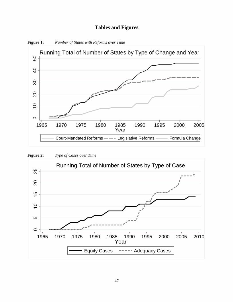
47  

Tables and Figures

Figure 1: Number of States with Reforms over Time

 Figure 2: Type of Cases over Time

 

01

02

03

04

05

0

1965 1970 1975 1980 1985 1990 1995 2000 2005Year

Court-Mandated Reforms Legislative Reforms Formula Change

Running Total of Number of States by Type of Change and Year

05

10

15

20

25

1965 1970 1975 1980 1985 1990 1995 2000 2005 2010Year

Equity Cases Adequacy Cases

Running Total of Number of States by Type of Case

 

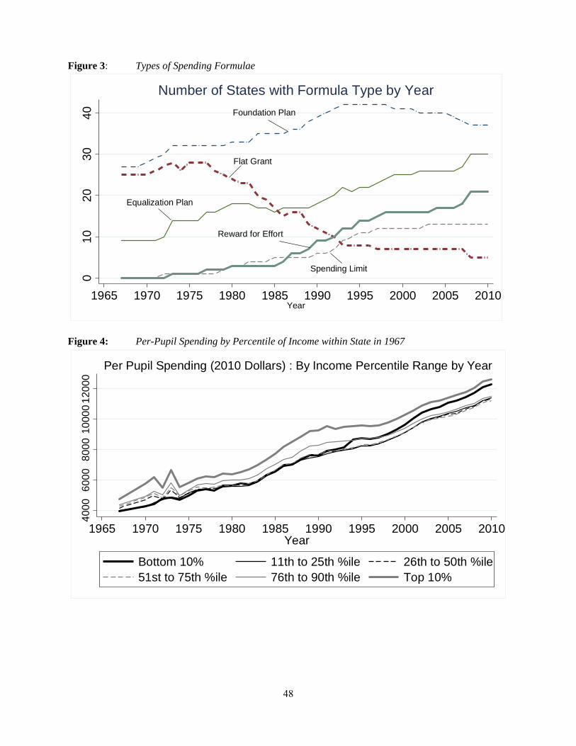
48  

Figure 3: Types of Spending Formulae

Figure 4: Per-Pupil Spending by Percentile of Income within State in 1967

Foundation Plan

Flat Grant

Equalization Plan

Spending Limit

Reward for Effort

010

2030

40

1965 1970 1975 1980 1985 1990 1995 2000 2005 2010Year

Number of States with Formula Type by Year4

000

600

08

000

1000

01

2000

1965 1970 1975 1980 1985 1990 1995 2000 2005 2010Year

Bottom 10% 11th to 25th %ile 26th to 50th %ile51st to 75th %ile 76th to 90th %ile Top 10%

Per Pupil Spending (2010 Dollars) : By Income Percentile Range by Year

 

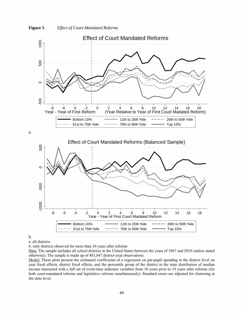
49  

Figure 5 Effect of Court-Mandated Reforms

a.

b. a: all districts b: only districts observed for more than 10 years after reforms Data: The sample includes all school districts in the United States between the years of 1967 and 2010 (unless stated otherwise). The sample is made up of 483,047 district-year observations. Model: These plots present the estimated coefficients of a regression on per-pupil spending at the district level on year fixed effects, district fixed effects, and the percentile group of the district in the state distribution of median income interacted with a full set of event-time indicator variables from 10 years prior to 19 years after reforms (for both court-mandated reforms and legislative reforms simultaneously). Standard errors are adjusted for clustering at the state level.   

-500

05

001

000

-8 -6 -4 -2 0 2 4 6 8 10 12 14 16 18Year - Year of First Reform (Year Relative to Year of First Court Madated Reform)

Bottom 10% 11th to 25th %ile 26th to 50th %ile51st to 75th %ile 76th to 90th %ile Top 10%

Effect of Court Mandated Reforms-1

000

-50

00

500

-8 -6 -4 -2 0 2 4 6 8 10 12 14 16 18Year - Year of First Court Madated Reform

Bottom 10% 11th to 25th %ile 26th to 50th %ile51st to 75th %ile 76th to 90th %ile Top 10%

Effect of Court Mandated Reforms (Balanced Sample)

 

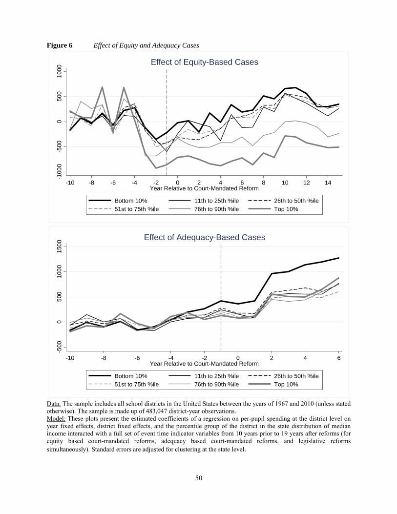
50  

Figure 6 Effect of Equity and Adequacy Cases

Data: The sample includes all school districts in the United States between the years of 1967 and 2010 (unless stated otherwise). The sample is made up of 483,047 district-year observations. Model: These plots present the estimated coefficients of a regression on per-pupil spending at the district level on year fixed effects, district fixed effects, and the percentile group of the district in the state distribution of median income interacted with a full set of event time indicator variables from 10 years prior to 19 years after reforms (for equity based court-mandated reforms, adequacy based court-mandated reforms, and legislative reforms simultaneously). Standard errors are adjusted for clustering at the state level.  

-100

0-5

000

500

100

0

-10 -8 -6 -4 -2 0 2 4 6 8 10 12 14Year Relative to Court-Mandated Reform

Bottom 10% 11th to 25th %ile 26th to 50th %ile51st to 75th %ile 76th to 90th %ile Top 10%

Effect of Equity-Based Cases-5

000

500

100

01

500

-10 -8 -6 -4 -2 0 2 4 6Year Relative to Court-Mandated Reform

Bottom 10% 11th to 25th %ile 26th to 50th %ile51st to 75th %ile 76th to 90th %ile Top 10%

Effect of Adequacy-Based Cases

 

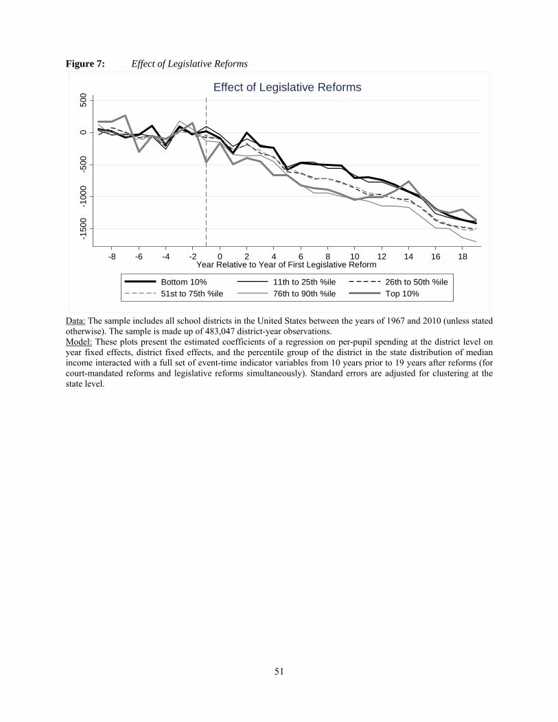
51  

Figure 7: Effect of Legislative Reforms

 Data: The sample includes all school districts in the United States between the years of 1967 and 2010 (unless stated otherwise). The sample is made up of 483,047 district-year observations. Model: These plots present the estimated coefficients of a regression on per-pupil spending at the district level on year fixed effects, district fixed effects, and the percentile group of the district in the state distribution of median income interacted with a full set of event-time indicator variables from 10 years prior to 19 years after reforms (for court-mandated reforms and legislative reforms simultaneously). Standard errors are adjusted for clustering at the state level.      

-150

0-1

000

-500

05

00

-8 -6 -4 -2 0 2 4 6 8 10 12 14 16 18Year Relative to Year of First Legislative Reform

Bottom 10% 11th to 25th %ile 26th to 50th %ile51st to 75th %ile 76th to 90th %ile Top 10%

Effect of Legislative Reforms

 

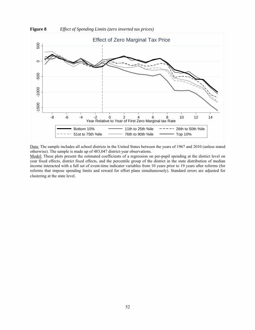
52  

Figure 8 Effect of Spending Limits (zero inverted tax prices)

 Data: The sample includes all school districts in the United States between the years of 1967 and 2010 (unless stated otherwise). The sample is made up of 483,047 district-year observations. Model: These plots present the estimated coefficients of a regression on per-pupil spending at the district level on year fixed effects, district fixed effects, and the percentile group of the district in the state distribution of median income interacted with a full set of event-time indicator variables from 10 years prior to 19 years after reforms (for reforms that impose spending limits and reward for effort plans simultaneously). Standard errors are adjusted for clustering at the state level.   

-150

0-1

000

-500

05

00

-8 -6 -4 -2 0 2 4 6 8 10 12 14Year Relative to Year of First Zero Marginal tax Rate

Bottom 10% 11th to 25th %ile 26th to 50th %ile51st to 75th %ile 76th to 90th %ile Top 10%

Effect of Zero Marginal Tax Price

 

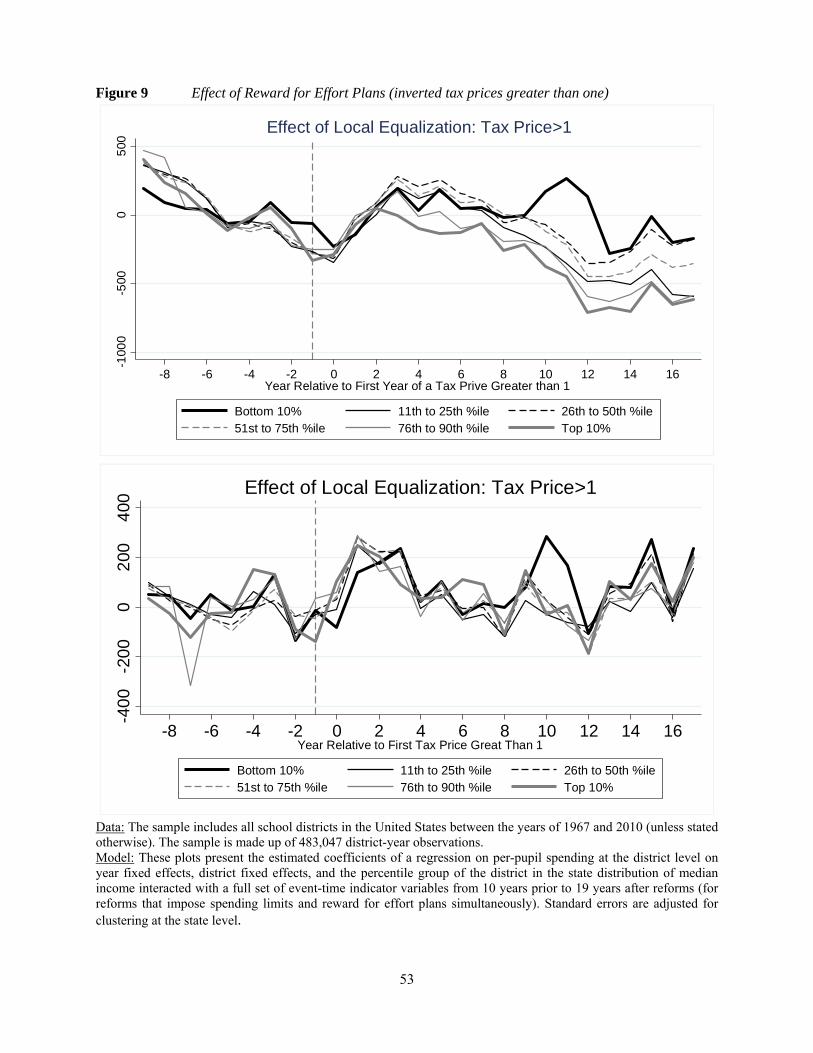
53  

Figure 9 Effect of Reward for Effort Plans (inverted tax prices greater than one)

 

Data: The sample includes all school districts in the United States between the years of 1967 and 2010 (unless stated otherwise). The sample is made up of 483,047 district-year observations. Model: These plots present the estimated coefficients of a regression on per-pupil spending at the district level on year fixed effects, district fixed effects, and the percentile group of the district in the state distribution of median income interacted with a full set of event-time indicator variables from 10 years prior to 19 years after reforms (for reforms that impose spending limits and reward for effort plans simultaneously). Standard errors are adjusted for clustering at the state level.   

-100

0-5

000

500

-8 -6 -4 -2 0 2 4 6 8 10 12 14 16Year Relative to First Year of a Tax Prive Greater than 1

Bottom 10% 11th to 25th %ile 26th to 50th %ile51st to 75th %ile 76th to 90th %ile Top 10%

Effect of Local Equalization: Tax Price>1-4

00

-20

00

200

400

-8 -6 -4 -2 0 2 4 6 8 10 12 14 16Year Relative to First Tax Price Great Than 1

Bottom 10% 11th to 25th %ile 26th to 50th %ile51st to 75th %ile 76th to 90th %ile Top 10%

Effect of Local Equalization: Tax Price>1

 

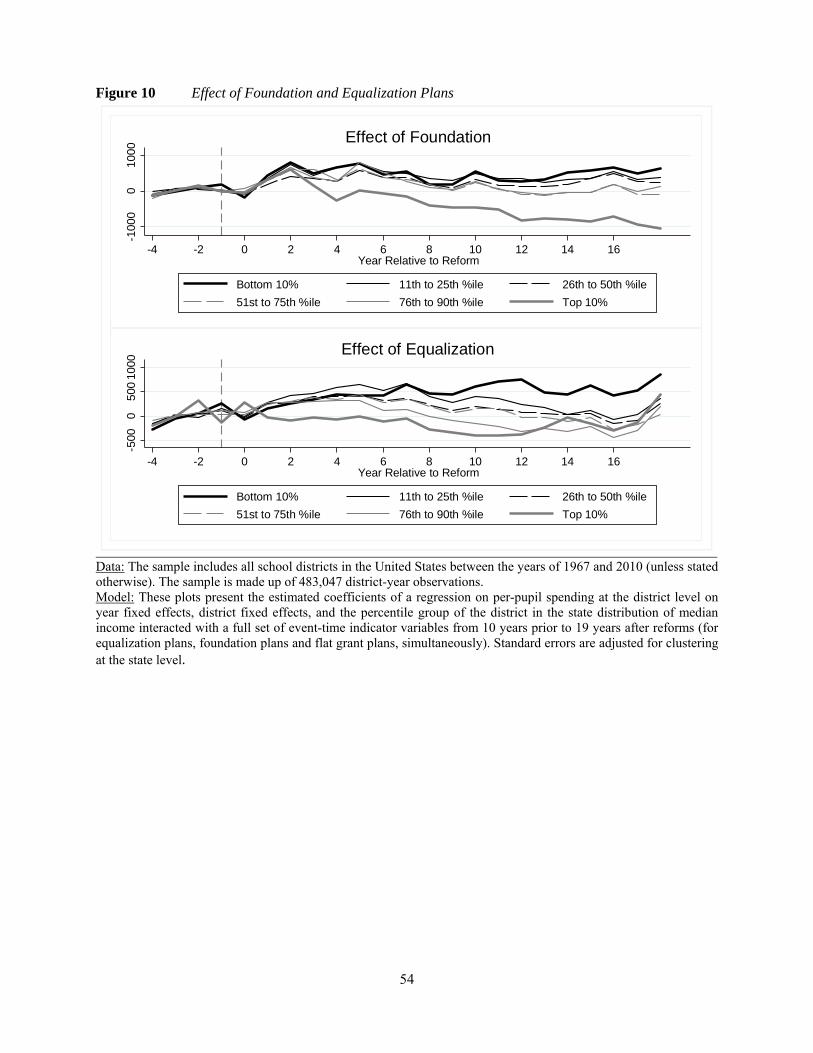
54  

Figure 10 Effect of Foundation and Equalization Plans 

Data: The sample includes all school districts in the United States between the years of 1967 and 2010 (unless stated otherwise). The sample is made up of 483,047 district-year observations. Model: These plots present the estimated coefficients of a regression on per-pupil spending at the district level on year fixed effects, district fixed effects, and the percentile group of the district in the state distribution of median income interacted with a full set of event-time indicator variables from 10 years prior to 19 years after reforms (for equalization plans, foundation plans and flat grant plans, simultaneously). Standard errors are adjusted for clustering at the state level.        

-100

00

1000

-4 -2 0 2 4 6 8 10 12 14 16Year Relative to Reform

Bottom 10% 11th to 25th %ile 26th to 50th %ile

51st to 75th %ile 76th to 90th %ile Top 10%

Effect of Foundation-5

000

500

1000

-4 -2 0 2 4 6 8 10 12 14 16Year Relative to Reform

Bottom 10% 11th to 25th %ile 26th to 50th %ile

51st to 75th %ile 76th to 90th %ile Top 10%

Effect of Equalization

 

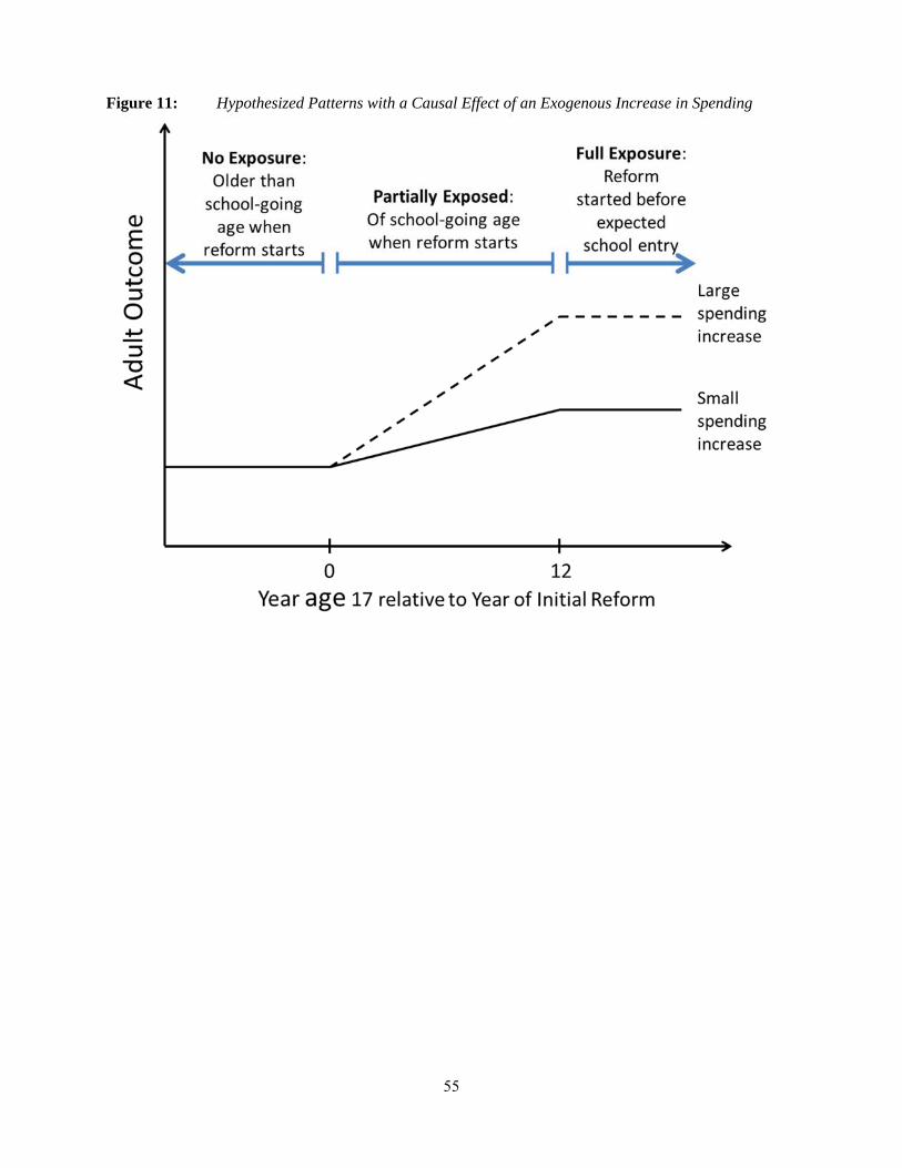
55  

Figure 11: Hypothesized Patterns with a Causal Effect of an Exogenous Increase in Spending

 

 

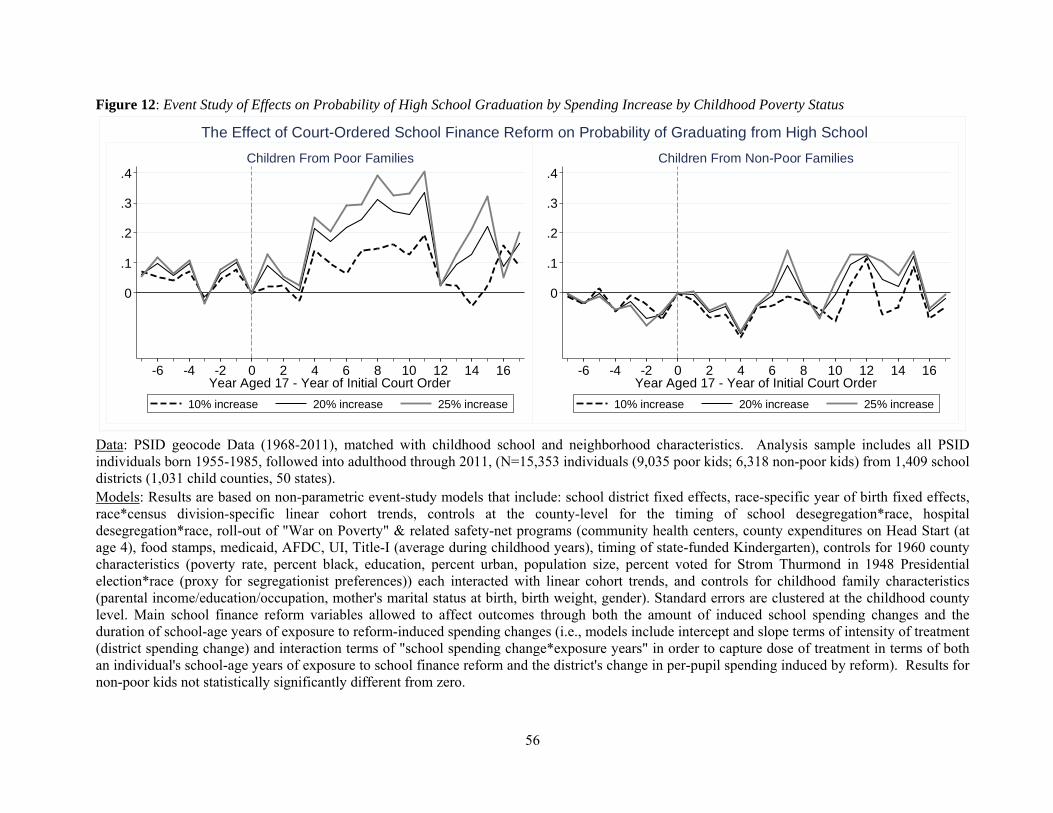
56  

Figure 12: Event Study of Effects on Probability of High School Graduation by Spending Increase by Childhood Poverty Status

Data: PSID geocode Data (1968-2011), matched with childhood school and neighborhood characteristics. Analysis sample includes all PSID individuals born 1955-1985, followed into adulthood through 2011, (N=15,353 individuals (9,035 poor kids; 6,318 non-poor kids) from 1,409 school districts (1,031 child counties, 50 states). Models: Results are based on non-parametric event-study models that include: school district fixed effects, race-specific year of birth fixed effects, race*census division-specific linear cohort trends, controls at the county-level for the timing of school desegregation*race, hospital desegregation*race, roll-out of "War on Poverty" & related safety-net programs (community health centers, county expenditures on Head Start (at age 4), food stamps, medicaid, AFDC, UI, Title-I (average during childhood years), timing of state-funded Kindergarten), controls for 1960 county characteristics (poverty rate, percent black, education, percent urban, population size, percent voted for Strom Thurmond in 1948 Presidential election*race (proxy for segregationist preferences)) each interacted with linear cohort trends, and controls for childhood family characteristics (parental income/education/occupation, mother's marital status at birth, birth weight, gender). Standard errors are clustered at the childhood county level. Main school finance reform variables allowed to affect outcomes through both the amount of induced school spending changes and the duration of school-age years of exposure to reform-induced spending changes (i.e., models include intercept and slope terms of intensity of treatment (district spending change) and interaction terms of "school spending change*exposure years" in order to capture dose of treatment in terms of both an individual's school-age years of exposure to school finance reform and the district's change in per-pupil spending induced by reform). Results for non-poor kids not statistically significantly different from zero.  

0

.1

.2

.3

.4

-6 -4 -2 0 2 4 6 8 10 12 14 16Year Aged 17 - Year of Initial Court Order

10% increase 20% increase 25% increase

Children From Non-Poor Families

0

.1

.2

.3

.4

-6 -4 -2 0 2 4 6 8 10 12 14 16Year Aged 17 - Year of Initial Court Order

10% increase 20% increase 25% increase

Children From Poor Families

The Effect of Court-Ordered School Finance Reform on Probability of Graduating from High School

 

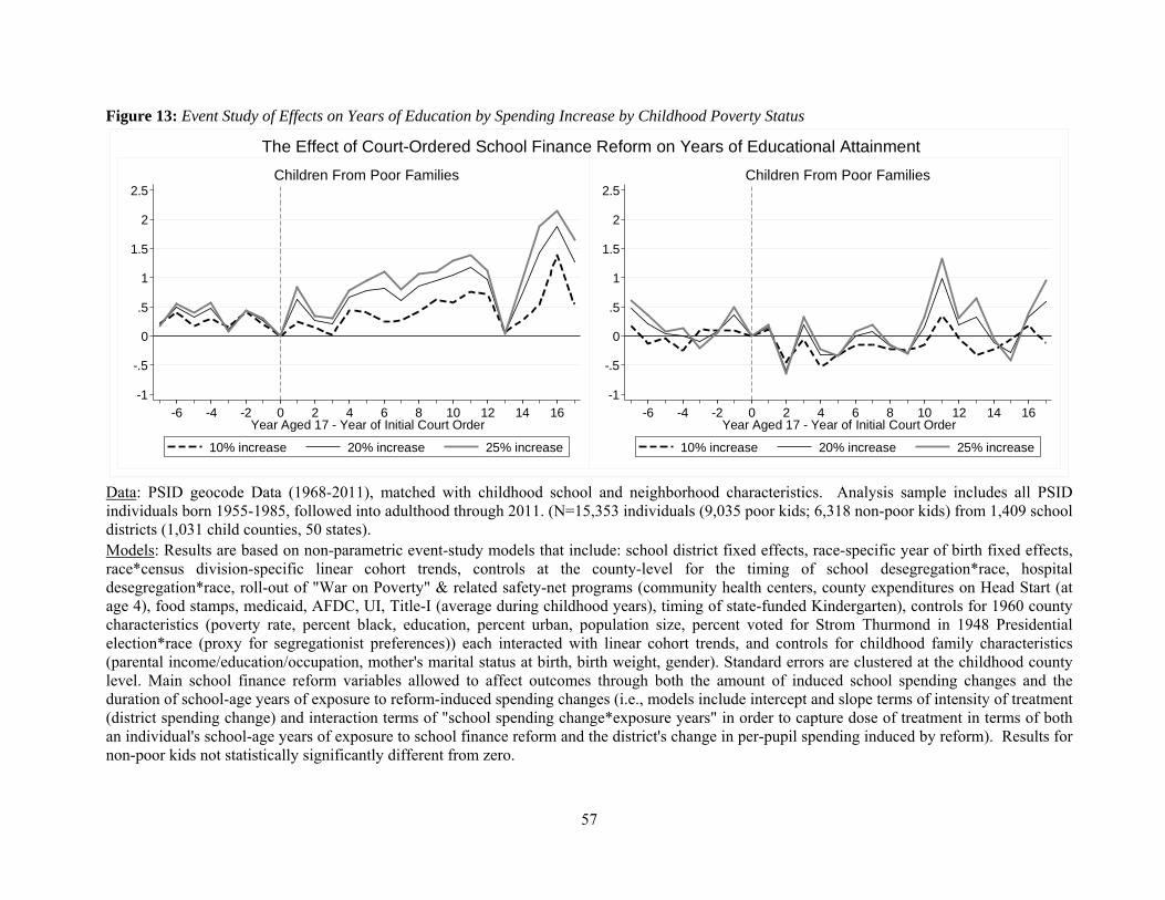
57  

Figure 13: Event Study of Effects on Years of Education by Spending Increase by Childhood Poverty Status

 Data: PSID geocode Data (1968-2011), matched with childhood school and neighborhood characteristics. Analysis sample includes all PSID individuals born 1955-1985, followed into adulthood through 2011. (N=15,353 individuals (9,035 poor kids; 6,318 non-poor kids) from 1,409 school districts (1,031 child counties, 50 states). Models: Results are based on non-parametric event-study models that include: school district fixed effects, race-specific year of birth fixed effects, race*census division-specific linear cohort trends, controls at the county-level for the timing of school desegregation*race, hospital desegregation*race, roll-out of "War on Poverty" & related safety-net programs (community health centers, county expenditures on Head Start (at age 4), food stamps, medicaid, AFDC, UI, Title-I (average during childhood years), timing of state-funded Kindergarten), controls for 1960 county characteristics (poverty rate, percent black, education, percent urban, population size, percent voted for Strom Thurmond in 1948 Presidential election*race (proxy for segregationist preferences)) each interacted with linear cohort trends, and controls for childhood family characteristics (parental income/education/occupation, mother's marital status at birth, birth weight, gender). Standard errors are clustered at the childhood county level. Main school finance reform variables allowed to affect outcomes through both the amount of induced school spending changes and the duration of school-age years of exposure to reform-induced spending changes (i.e., models include intercept and slope terms of intensity of treatment (district spending change) and interaction terms of "school spending change*exposure years" in order to capture dose of treatment in terms of both an individual's school-age years of exposure to school finance reform and the district's change in per-pupil spending induced by reform). Results for non-poor kids not statistically significantly different from zero.

-1

-.5

0

.5

1

1.5

2

2.5

-6 -4 -2 0 2 4 6 8 10 12 14 16Year Aged 17 - Year of Initial Court Order

10% increase 20% increase 25% increase

Children From Poor Families

-1

-.5

0

.5

1

1.5

2

2.5

-6 -4 -2 0 2 4 6 8 10 12 14 16Year Aged 17 - Year of Initial Court Order

10% increase 20% increase 25% increase

Children From Poor Families

The Effect of Court-Ordered School Finance Reform on Years of Educational Attainment

 

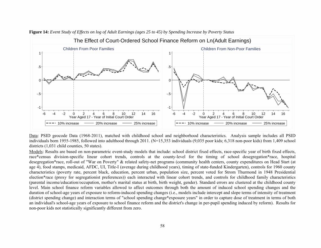
58  

Figure 14: Event Study of Effects on log of Adult Earnings (ages 25 to 45) by Spending Increase by Poverty Status 

 Data: PSID geocode Data (1968-2011), matched with childhood school and neighborhood characteristics. Analysis sample includes all PSID individuals born 1955-1985, followed into adulthood through 2011. (N=15,353 individuals (9,035 poor kids; 6,318 non-poor kids) from 1,409 school districts (1,031 child counties, 50 states). Models: Results are based on non-parametric event-study models that include: school district fixed effects, race-specific year of birth fixed effects, race*census division-specific linear cohort trends, controls at the county-level for the timing of school desegregation*race, hospital desegregation*race, roll-out of "War on Poverty" & related safety-net programs (community health centers, county expenditures on Head Start (at age 4), food stamps, medicaid, AFDC, UI, Title-I (average during childhood years), timing of state-funded Kindergarten), controls for 1960 county characteristics (poverty rate, percent black, education, percent urban, population size, percent voted for Strom Thurmond in 1948 Presidential election*race (proxy for segregationist preferences)) each interacted with linear cohort trends, and controls for childhood family characteristics (parental income/education/occupation, mother's marital status at birth, birth weight, gender). Standard errors are clustered at the childhood county level. Main school finance reform variables allowed to affect outcomes through both the amount of induced school spending changes and the duration of school-age years of exposure to reform-induced spending changes (i.e., models include intercept and slope terms of intensity of treatment (district spending change) and interaction terms of "school spending change*exposure years" in order to capture dose of treatment in terms of both an individual's school-age years of exposure to school finance reform and the district's change in per-pupil spending induced by reform). Results for non-poor kids not statistically significantly different from zero.

-1

-.5

0

.5

1

-6 -4 -2 0 2 4 6 8 10 12 14 16Year Aged 17 - Year of Initial Court Order

10% increase 20% increase 25% increase

Children From Non-Poor Families

-1

-.5

0

.5

1

-6 -4 -2 0 2 4 6 8 10 12 14 16Year Aged 17 - Year of Initial Court Order

10% increase 20% increase 25% increase

Children From Poor Families

The Effect of Court-Ordered School Finance Reform on Ln(Adult Earnings)

 

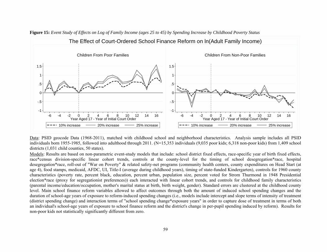
59  

Figure 15: Event Study of Effects on Log of Family Income (ages 25 to 45) by Spending Increase by Childhood Poverty Status

   Data: PSID geocode Data (1968-2011), matched with childhood school and neighborhood characteristics. Analysis sample includes all PSID individuals born 1955-1985, followed into adulthood through 2011. (N=15,353 individuals (9,035 poor kids; 6,318 non-poor kids) from 1,409 school districts (1,031 child counties, 50 states). Models: Results are based on non-parametric event-study models that include: school district fixed effects, race-specific year of birth fixed effects, race*census division-specific linear cohort trends, controls at the county-level for the timing of school desegregation*race, hospital desegregation*race, roll-out of "War on Poverty" & related safety-net programs (community health centers, county expenditures on Head Start (at age 4), food stamps, medicaid, AFDC, UI, Title-I (average during childhood years), timing of state-funded Kindergarten), controls for 1960 county characteristics (poverty rate, percent black, education, percent urban, population size, percent voted for Strom Thurmond in 1948 Presidential election*race (proxy for segregationist preferences)) each interacted with linear cohort trends, and controls for childhood family characteristics (parental income/education/occupation, mother's marital status at birth, birth weight, gender). Standard errors are clustered at the childhood county level. Main school finance reform variables allowed to affect outcomes through both the amount of induced school spending changes and the duration of school-age years of exposure to reform-induced spending changes (i.e., models include intercept and slope terms of intensity of treatment (district spending change) and interaction terms of "school spending change*exposure years" in order to capture dose of treatment in terms of both an individual's school-age years of exposure to school finance reform and the district's change in per-pupil spending induced by reform). Results for non-poor kids not statistically significantly different from zero.  

-1

-.5

0

.5

1

1.5

-6 -4 -2 0 2 4 6 8 10 12 14 16Year Aged 17 - Year of Initial Court Order

10% increase 20% increase 25% increase

Children From Non-Poor Families

-1

-.5

0

.5

1

1.5

-6 -4 -2 0 2 4 6 8 10 12 14 16Year Aged 17 - Year of Initial Court Order

10% increase 20% increase 25% increase

Children From Poor Families

The Effect of Court-Ordered School Finance Reform on ln(Adult Family Income)

 

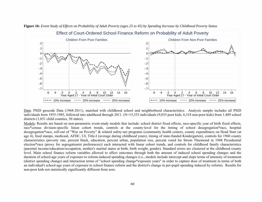
60  

Figure 16: Event Study of Effects on Probability of Adult Poverty (ages 25 to 45) by Spending Increase by Childhood Poverty Status

  Data: PSID geocode Data (1968-2011), matched with childhood school and neighborhood characteristics. Analysis sample includes all PSID individuals born 1955-1985, followed into adulthood through 2011. (N=15,353 individuals (9,035 poor kids; 6,318 non-poor kids) from 1,409 school districts (1,031 child counties, 50 states). Models: Results are based on non-parametric event-study models that include: school district fixed effects, race-specific year of birth fixed effects, race*census division-specific linear cohort trends, controls at the county-level for the timing of school desegregation*race, hospital desegregation*race, roll-out of "War on Poverty" & related safety-net programs (community health centers, county expenditures on Head Start (at age 4), food stamps, medicaid, AFDC, UI, Title-I (average during childhood years), timing of state-funded Kindergarten), controls for 1960 county characteristics (poverty rate, percent black, education, percent urban, population size, percent voted for Strom Thurmond in 1948 Presidential election*race (proxy for segregationist preferences)) each interacted with linear cohort trends, and controls for childhood family characteristics (parental income/education/occupation, mother's marital status at birth, birth weight, gender). Standard errors are clustered at the childhood county level. Main school finance reform variables allowed to affect outcomes through both the amount of induced school spending changes and the duration of school-age years of exposure to reform-induced spending changes (i.e., models include intercept and slope terms of intensity of treatment (district spending change) and interaction terms of "school spending change*exposure years" in order to capture dose of treatment in terms of both an individual's school-age years of exposure to school finance reform and the district's change in per-pupil spending induced by reform). Results for non-poor kids not statistically significantly different from zero.

-.7

-.6

-.5

-.4

-.3

-.2

-.1

0

.1

.2

-6 -4 -2 0 2 4 6 8 10 12 14 16Year Aged 17 - Year of Initial Court Order

10% increase 20% increase 25% increase

Children From Non-Poor Families

-.7

-.6

-.5

-.4

-.3

-.2

-.1

0

.1

.2

-6 -4 -2 0 2 4 6 8 10 12 14 16Year Aged 17 - Year of Initial Court Order

10% increase 20% increase 25% increase

Children From Poor Families

Effect of Court-Ordered School Finance Reform on Probability of Adult Poverty

 

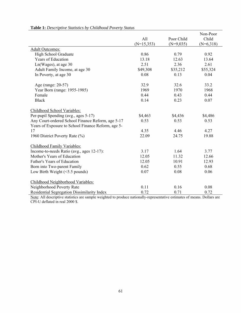
61  

Table 1: Descriptive Statistics by Childhood Poverty Status

All (N=15,353)

Poor Child (N=9,035)

Non-Poor Child

(N=6,318) Adult Outcomes:

High School Graduate 0.86 0.79 0.92 Years of Education 13.18 12.63 13.64 Ln(Wages), at age 30 2.51 2.36 2.61 Adult Family Income, at age 30 $49,308 $35,212 $55,324 In Poverty, at age 30 0.08 0.13 0.04

Age (range: 20-57) 32.9 32.6 33.2 Year Born (range: 1955-1985) 1969 1970 1968 Female 0.44 0.43 0.44 Black 0.14 0.23 0.07

Childhood School Variables: Per-pupil Spending (avg., ages 5-17) $4,463 $4,436 $4,486 Any Court-ordered School Finance Reform, age 5-17 0.53 0.53 0.53 Years of Exposure to School Finance Reform, age 5-17 4.35 4.46 4.27 1960 District Poverty Rate (%) 22.09 24.75 19.88

Childhood Family Variables: Income-to-needs Ratio (avg., ages 12-17): 3.17 1.64 3.77 Mother's Years of Education 12.05 11.32 12.66 Father's Years of Education 12.05 10.91 12.93 Born into Two-parent Family 0.62 0.55 0.68 Low Birth Weight (<5.5 pounds) 0.07 0.08 0.06

Childhood Neighborhood Variables: Neighborhood Poverty Rate 0.11 0.16 0.08 Residential Segregation Dissimilarity Index 0.72 0.71 0.72 Note: All descriptive statistics are sample weighted to produce nationally-representative estimates of means. Dollars are CPI-U deflated in real 2000 $.

62

Table 2: OLS vs 2SLS Estimates of Court-Ordered School Finance Reform Induced Effects of Per-Pupil Spending on Educational Attainment: by Childhood Poverty Status

All Children (Population weighted) Children from Poor Families

Children from Non-Poor Families

OLS 2SLS/IV OLS 2SLS/IV OLS 2SLS/IV(1) (2) (3) (4) (5) (6)

Dependent variable: Prob(HS Grad)

Ln(School District Per-pupil Spending)(age 5-17) 0.0095* 0.1475*** 0.0010 0.2293*** 0.0044 0.0647 (0.0052) (0.0410) (0.0069) (0.0726) (0.0065) (0.0526)

Dependent variable: Years of Education

Ln(School District Per-pupil Spending)(age 5-17) 0.0077 0.7599*** -0.0247 0.9282*** -0.0135 0.2959(0.0325) (0.2483) (0.0314) (0.2872) (0.0373) (0.3284)

Number of Individuals 14,670 14,670 8,639 8,639 6,031 6,031 Number of School Districts 1,288 1,288 918 918 978 978 *** p<0.01, ** p<0.05, * p<0.10 Robust standard errors in parentheses (clustered at school district level) Data: PSID geocode Data (1968-2011), matched with childhood school and neighborhood characteristics. Analysis sample includes all PSID individuals born 1955-1985, followed into adulthood through 2011.Models: Results are based on OLS and 2SLS/IV models that include: school district fixed effects, race-specific year of birth fixed effects, race*census division-specific linear cohort trends; controls at the county-level for the timing of school desegregation*race, hospital desegregation*race, roll-out of "War on Poverty" & related safety-net programs (community health centers, county expenditures on Head Start (at age 4), food stamps, medicaid, AFDC, UI, Title-I (average during childhood years), timing of state-funded Kindergarten intro); controls for 1960 county characteristics (poverty rate, percent black, education, percent urban, population size, percent voted for Strom Thurmond in 1948 Presidential election*race (proxy for segregationist preferences)) each interacted with linear cohort trends; and controls for childhood family characteristics (parental income/education/occupation, mother's marital status at birth, birth weight, gender). PSID sample weights are used to account for oversampling of poor families to produce nationally-representative estimates for models with all kids. The first-stage model includes as predictors the school-age years of exposure to school finance reform interacted with the respective school district's reform-induced change in school spending. There exists a significant first-stage for both poor and non-poor kids.

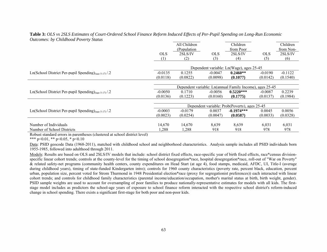
63

Table 3: OLS vs 2SLS Estimates of Court-Ordered School Finance Reform Induced Effects of Per-Pupil Spending on Long-Run Economic Outcomes: by Childhood Poverty Status

All Children (Population

Children from Poor

Children from Non-

OLS 2SLS/IV OLS 2SLS/IV OLS 2SLS/IV(1) (2) (3) (4) (5) (6)

Dependent variable: Ln(Wage), ages 25-45

Ln(School District Per-pupil Spending)(age 5-17) /.2 -0.0135 0.1255 -0.0047 0.2460** -0.0190 -0.1122 (0.0118) (0.0822) (0.0098) (0.1077) (0.0142) (0.1540)

Dependent variable: Ln(annual Family Income), ages 25-45Ln(School District Per-pupil Spending)(age 5-17) /.2 -0.0050 0.1710 -0.0056 0.5220*** -0.0087 0.2239 (0.0136) (0.1223) (0.0160) (0.1775) (0.0137) (0.1984)

Dependent variable: Prob(Poverty), ages 25-45Ln(School District Per-pupil Spending)(age 5-17) /.2 -0.0003 -0.0179 0.0037 -0.1974*** 0.0045 0.0056

(0.0023) (0.0254) (0.0047) (0.0587) (0.0033) (0.0328)

Number of Individuals 14,670 14,670 8,639 8,639 6,031 6,031 Number of School Districts 1,288 1,288 918 918 978 978 Robust standard errors in parentheses (clustered at school district level)*** p<0.01, ** p<0.05, * p<0.10 Data: PSID geocode Data (1968-2011), matched with childhood school and neighborhood characteristics. Analysis sample includes all PSID individuals born 1955-1985, followed into adulthood through 2011. Models: Results are based on OLS and 2SLS/IV models that include: school district fixed effects, race-specific year of birth fixed effects, race*census division-specific linear cohort trends; controls at the county-level for the timing of school desegregation*race, hospital desegregation*race, roll-out of "War on Poverty" & related safety-net programs (community health centers, county expenditures on Head Start (at age 4), food stamps, medicaid, AFDC, UI, Title-I (average during childhood years), timing of state-funded Kindergarten intro); controls for 1960 county characteristics (poverty rate, percent black, education, percent urban, population size, percent voted for Strom Thurmond in 1948 Presidential election*race (proxy for segregationist preferences)) each interacted with linear cohort trends; and controls for childhood family characteristics (parental income/education/occupation, mother's marital status at birth, birth weight, gender). PSID sample weights are used to account for oversampling of poor families to produce nationally-representative estimates for models with all kids. The first-stage model includes as predictors the school-age years of exposure to school finance reform interacted with the respective school district's reform-induced change in school spending. There exists a significant first-stage for both poor and non-poor kids.

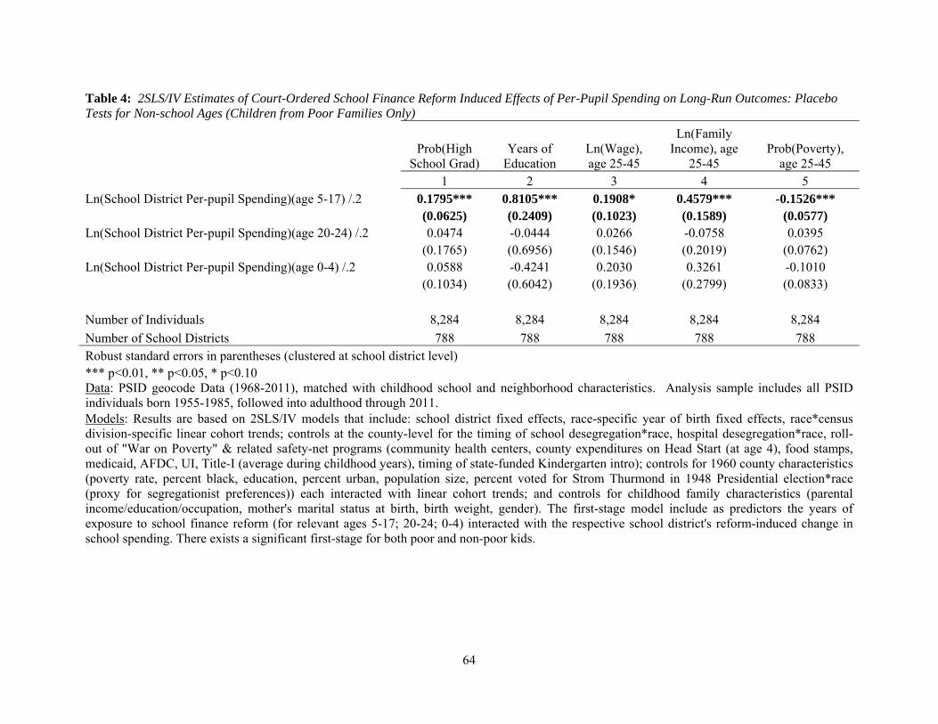
64

Table 4: 2SLS/IV Estimates of Court-Ordered School Finance Reform Induced Effects of Per-Pupil Spending on Long-Run Outcomes: Placebo Tests for Non-school Ages (Children from Poor Families Only)

Prob(High School Grad)

Years of Education

Ln(Wage), age 25-45

Ln(Family Income), age

25-45 Prob(Poverty),

age 25-45 1 2 3 4 5

Ln(School District Per-pupil Spending)(age 5-17) /.2 0.1795*** 0.8105*** 0.1908* 0.4579*** -0.1526*** (0.0625) (0.2409) (0.1023) (0.1589) (0.0577)

Ln(School District Per-pupil Spending)(age 20-24) /.2 0.0474 -0.0444 0.0266 -0.0758 0.0395 (0.1765) (0.6956) (0.1546) (0.2019) (0.0762)

Ln(School District Per-pupil Spending)(age 0-4) /.2 0.0588 -0.4241 0.2030 0.3261 -0.1010 (0.1034) (0.6042) (0.1936) (0.2799) (0.0833)

Number of Individuals 8,284 8,284 8,284 8,284 8,284 Number of School Districts 788 788 788 788 788 Robust standard errors in parentheses (clustered at school district level) *** p<0.01, ** p<0.05, * p<0.10 Data: PSID geocode Data (1968-2011), matched with childhood school and neighborhood characteristics. Analysis sample includes all PSID individuals born 1955-1985, followed into adulthood through 2011. Models: Results are based on 2SLS/IV models that include: school district fixed effects, race-specific year of birth fixed effects, race*census division-specific linear cohort trends; controls at the county-level for the timing of school desegregation*race, hospital desegregation*race, roll-out of "War on Poverty" & related safety-net programs (community health centers, county expenditures on Head Start (at age 4), food stamps, medicaid, AFDC, UI, Title-I (average during childhood years), timing of state-funded Kindergarten intro); controls for 1960 county characteristics (poverty rate, percent black, education, percent urban, population size, percent voted for Strom Thurmond in 1948 Presidential election*race (proxy for segregationist preferences)) each interacted with linear cohort trends; and controls for childhood family characteristics (parental income/education/occupation, mother's marital status at birth, birth weight, gender). The first-stage model include as predictors the years of exposure to school finance reform (for relevant ages 5-17; 20-24; 0-4) interacted with the respective school district's reform-induced change in school spending. There exists a significant first-stage for both poor and non-poor kids.

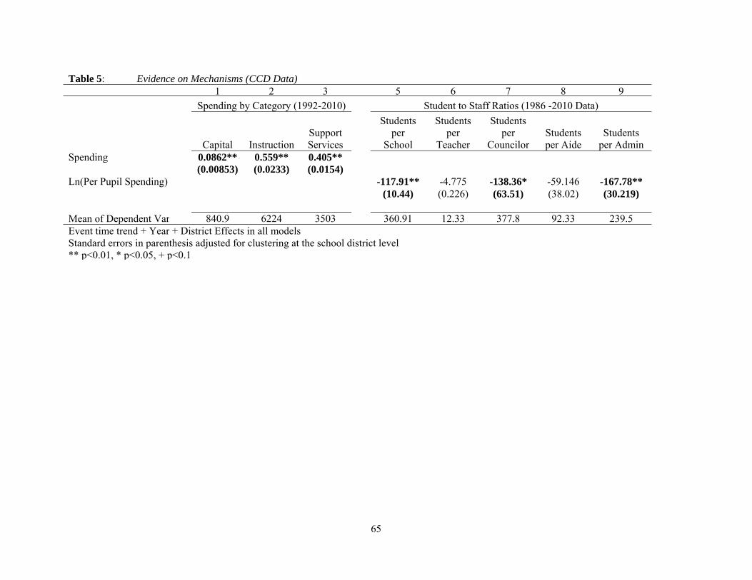
65

Table 5: Evidence on Mechanisms (CCD Data) 1 2 3 5 6 7 8 9

Spending by Category (1992-2010) Student to Staff Ratios (1986 -2010 Data)

Capital InstructionSupport Services

Students per

School

Students per

Teacher

Students per

Councilor Students per Aide

Students per Admin

Spending 0.0862** 0.559** 0.405** (0.00853) (0.0233) (0.0154)

Ln(Per Pupil Spending) -117.91** -4.775 -138.36* -59.146 -167.78** (10.44) (0.226) (63.51) (38.02) (30.219)

Mean of Dependent Var 840.9 6224 3503 360.91 12.33 377.8 92.33 239.5Event time trend + Year + District Effects in all modelsStandard errors in parenthesis adjusted for clustering at the school district level ** p<0.01, * p<0.05, + p<0.1

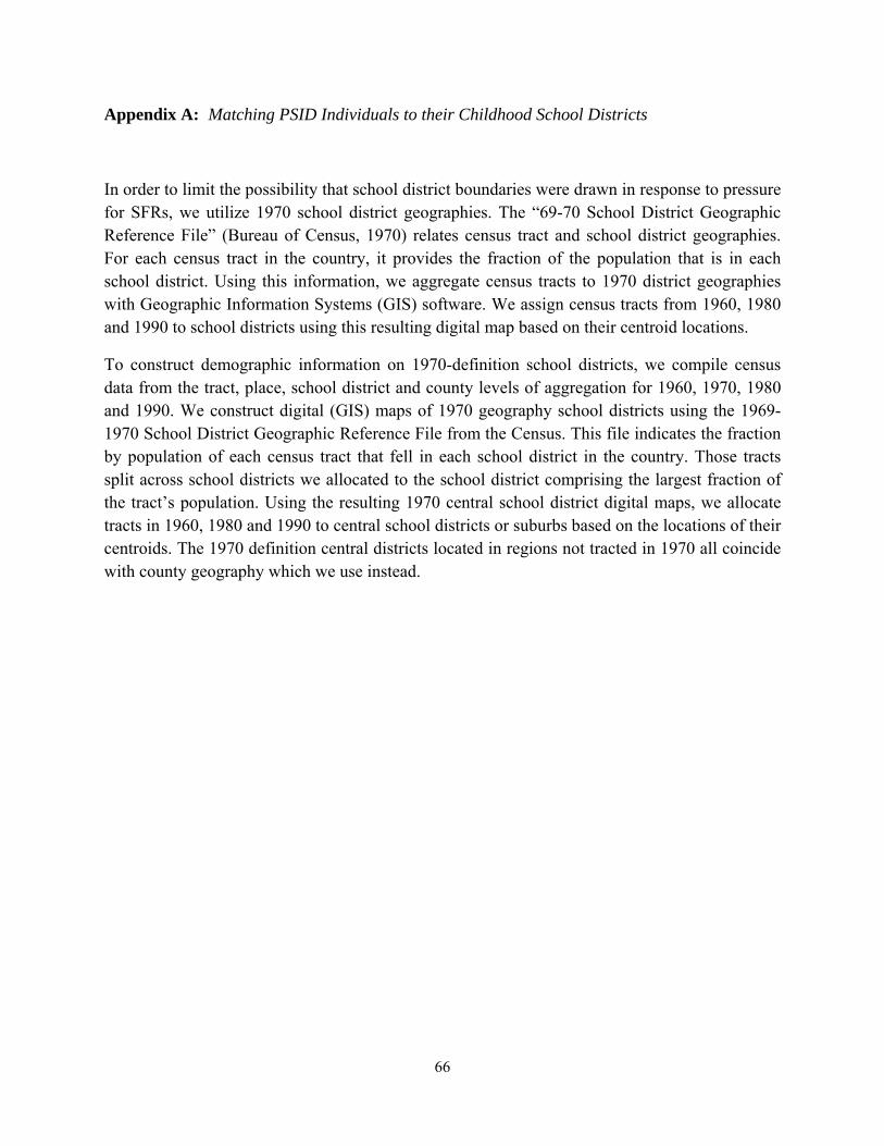
66

Appendix A: Matching PSID Individuals to their Childhood School Districts

In order to limit the possibility that school district boundaries were drawn in response to pressure for SFRs, we utilize 1970 school district geographies. The “69-70 School District Geographic Reference File” (Bureau of Census, 1970) relates census tract and school district geographies. For each census tract in the country, it provides the fraction of the population that is in each school district. Using this information, we aggregate census tracts to 1970 district geographies with Geographic Information Systems (GIS) software. We assign census tracts from 1960, 1980 and 1990 to school districts using this resulting digital map based on their centroid locations.

To construct demographic information on 1970-definition school districts, we compile census data from the tract, place, school district and county levels of aggregation for 1960, 1970, 1980 and 1990. We construct digital (GIS) maps of 1970 geography school districts using the 1969-1970 School District Geographic Reference File from the Census. This file indicates the fraction by population of each census tract that fell in each school district in the country. Those tracts split across school districts we allocated to the school district comprising the largest fraction of the tract’s population. Using the resulting 1970 central school district digital maps, we allocate tracts in 1960, 1980 and 1990 to central school districts or suburbs based on the locations of their centroids. The 1970 definition central districts located in regions not tracted in 1970 all coincide with county geography which we use instead.

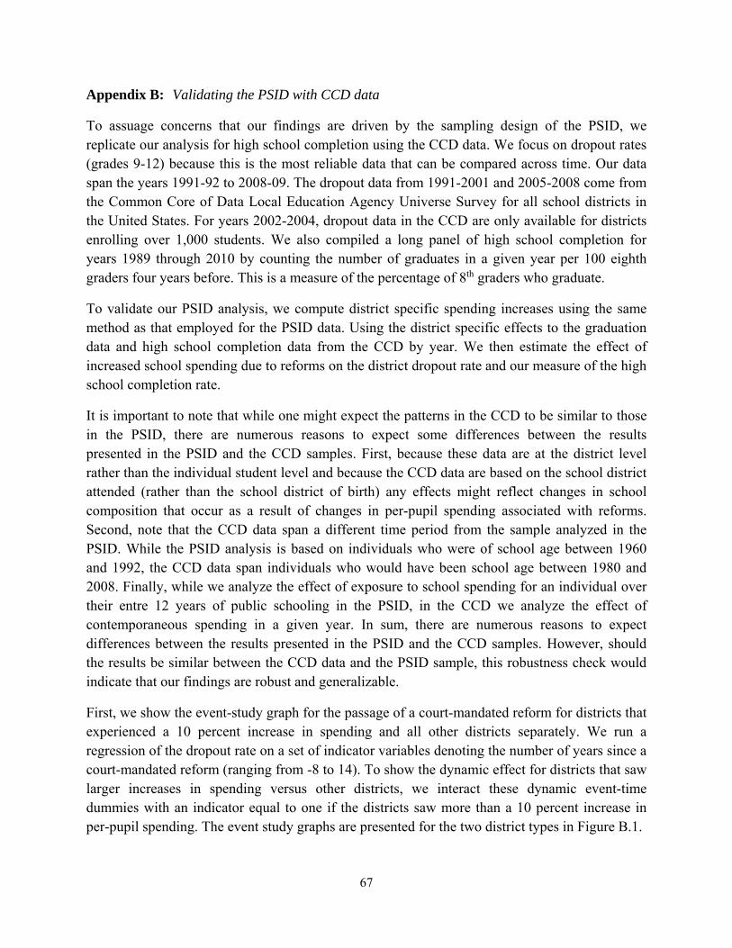
67

Appendix B: Validating the PSID with CCD data

To assuage concerns that our findings are driven by the sampling design of the PSID, we replicate our analysis for high school completion using the CCD data. We focus on dropout rates (grades 9-12) because this is the most reliable data that can be compared across time. Our data span the years 1991-92 to 2008-09. The dropout data from 1991-2001 and 2005-2008 come from the Common Core of Data Local Education Agency Universe Survey for all school districts in the United States. For years 2002-2004, dropout data in the CCD are only available for districts enrolling over 1,000 students. We also compiled a long panel of high school completion for years 1989 through 2010 by counting the number of graduates in a given year per 100 eighth graders four years before. This is a measure of the percentage of 8th graders who graduate.

To validate our PSID analysis, we compute district specific spending increases using the same method as that employed for the PSID data. Using the district specific effects to the graduation data and high school completion data from the CCD by year. We then estimate the effect of increased school spending due to reforms on the district dropout rate and our measure of the high school completion rate.

It is important to note that while one might expect the patterns in the CCD to be similar to those in the PSID, there are numerous reasons to expect some differences between the results presented in the PSID and the CCD samples. First, because these data are at the district level rather than the individual student level and because the CCD data are based on the school district attended (rather than the school district of birth) any effects might reflect changes in school composition that occur as a result of changes in per-pupil spending associated with reforms. Second, note that the CCD data span a different time period from the sample analyzed in the PSID. While the PSID analysis is based on individuals who were of school age between 1960 and 1992, the CCD data span individuals who would have been school age between 1980 and 2008. Finally, while we analyze the effect of exposure to school spending for an individual over their entre 12 years of public schooling in the PSID, in the CCD we analyze the effect of contemporaneous spending in a given year. In sum, there are numerous reasons to expect differences between the results presented in the PSID and the CCD samples. However, should the results be similar between the CCD data and the PSID sample, this robustness check would indicate that our findings are robust and generalizable.

First, we show the event-study graph for the passage of a court-mandated reform for districts that experienced a 10 percent increase in spending and all other districts separately. We run a regression of the dropout rate on a set of indicator variables denoting the number of years since a court-mandated reform (ranging from -8 to 14). To show the dynamic effect for districts that saw larger increases in spending versus other districts, we interact these dynamic event-time dummies with an indicator equal to one if the districts saw more than a 10 percent increase in per-pupil spending. The event study graphs are presented for the two district types in Figure B.1.

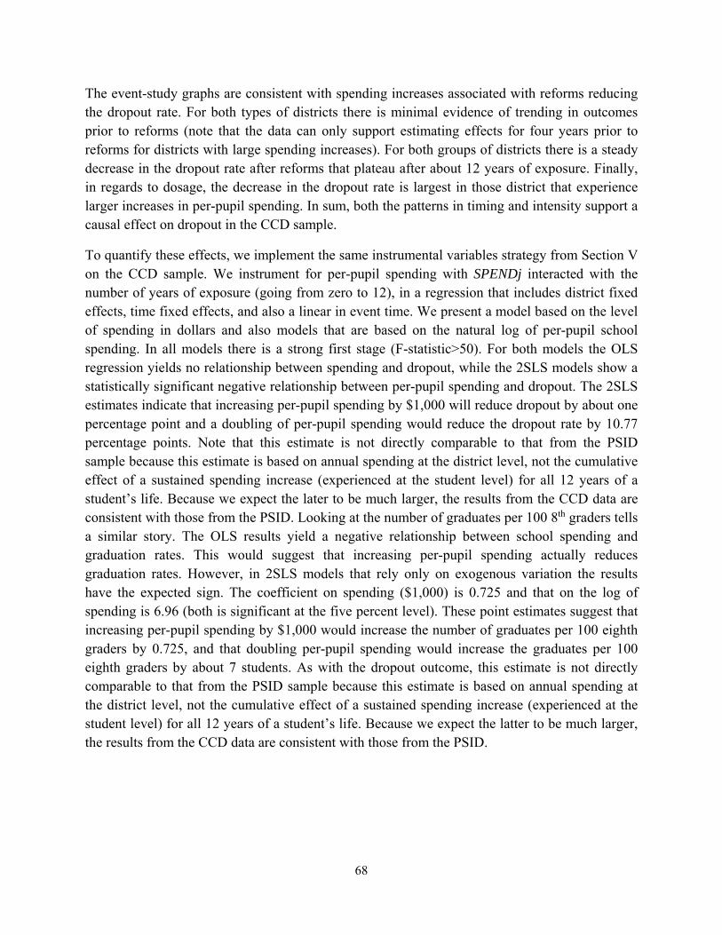
68

The event-study graphs are consistent with spending increases associated with reforms reducing the dropout rate. For both types of districts there is minimal evidence of trending in outcomes prior to reforms (note that the data can only support estimating effects for four years prior to reforms for districts with large spending increases). For both groups of districts there is a steady decrease in the dropout rate after reforms that plateau after about 12 years of exposure. Finally, in regards to dosage, the decrease in the dropout rate is largest in those district that experience larger increases in per-pupil spending. In sum, both the patterns in timing and intensity support a causal effect on dropout in the CCD sample.

To quantify these effects, we implement the same instrumental variables strategy from Section V on the CCD sample. We instrument for per-pupil spending with SPENDj interacted with the number of years of exposure (going from zero to 12), in a regression that includes district fixed effects, time fixed effects, and also a linear in event time. We present a model based on the level of spending in dollars and also models that are based on the natural log of per-pupil school spending. In all models there is a strong first stage (F-statistic>50). For both models the OLS regression yields no relationship between spending and dropout, while the 2SLS models show a statistically significant negative relationship between per-pupil spending and dropout. The 2SLS estimates indicate that increasing per-pupil spending by $1,000 will reduce dropout by about one percentage point and a doubling of per-pupil spending would reduce the dropout rate by 10.77 percentage points. Note that this estimate is not directly comparable to that from the PSID sample because this estimate is based on annual spending at the district level, not the cumulative effect of a sustained spending increase (experienced at the student level) for all 12 years of a student’s life. Because we expect the later to be much larger, the results from the CCD data are consistent with those from the PSID. Looking at the number of graduates per 100 8th graders tells a similar story. The OLS results yield a negative relationship between school spending and graduation rates. This would suggest that increasing per-pupil spending actually reduces graduation rates. However, in 2SLS models that rely only on exogenous variation the results have the expected sign. The coefficient on spending ($1,000) is 0.725 and that on the log of spending is 6.96 (both is significant at the five percent level). These point estimates suggest that increasing per-pupil spending by $1,000 would increase the number of graduates per 100 eighth graders by 0.725, and that doubling per-pupil spending would increase the graduates per 100 eighth graders by about 7 students. As with the dropout outcome, this estimate is not directly comparable to that from the PSID sample because this estimate is based on annual spending at the district level, not the cumulative effect of a sustained spending increase (experienced at the student level) for all 12 years of a student’s life. Because we expect the latter to be much larger, the results from the CCD data are consistent with those from the PSID.

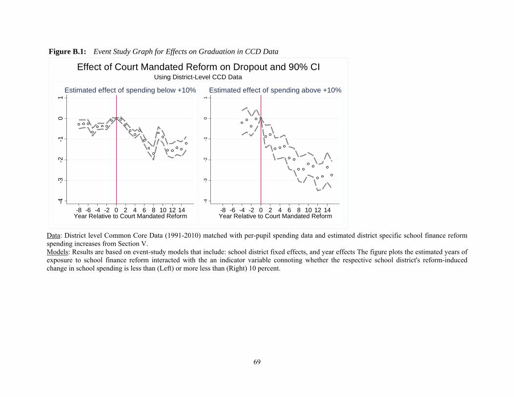
69

Figure B.1: Event Study Graph for Effects on Graduation in CCD Data

 Data: District level Common Core Data (1991-2010) matched with per-pupil spending data and estimated district specific school finance reform spending increases from Section V. Models: Results are based on event-study models that include: school district fixed effects, and year effects The figure plots the estimated years of exposure to school finance reform interacted with the an indicator variable connoting whether the respective school district's reform-induced change in school spending is less than (Left) or more less than (Right) 10 percent.  

-4-3

-2-1

01

-8 -6 -4 -2 0 2 4 6 8 10 12 14Year Relative to Court Mandated Reform

Estimated effect of spending below +10%

-4-3

-2-1

01

-8 -6 -4 -2 0 2 4 6 8 10 12 14Year Relative to Court Mandated Reform

Estimated effect of spending above +10%

Using District-Level CCD Data

Effect of Court Mandated Reform on Dropout and 90% CI

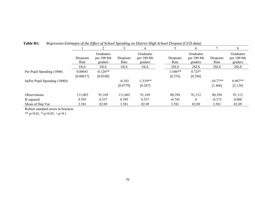
70

Table B1: Regression Estimates of the Effect of School Spending on District High School Dropout (CCD data)

1 2 3 4 5 6 7 8

Dropouts Rate

Graduates per 100 8th

graders Dropouts

Rate

Graduates per 100 8th

graders Dropouts

Rate

Graduates per 100 8th

graders Dropouts

Rate

Graduates per 100 8th

graders OLS OLS OLS OLS 2SLS 2SLS 2SLS 2SLS

Per Pupil Spending (1000) 0.00641 -0.126** -1.046** 0.725* [0.00617] [0.0248] [0.276] [0.296]

ln(Per Pupil Spending (1000)) -0.103 -1.519** -10.77** 6.967** [0.0779] [0.287] [1.466] [2.138]

Observations 111,065 91,169 111,065 91,169 80,394 91,112 80,394 91,112 R-squared 0.595 0.537 0.595 0.537 -0.745 0 -0.373 0.008 Mean of Dep Var 3.581 82.09 3.581 82.09 3.581 82.09 3.581 82.09 Robust standard errors in brackets ** p<0.01, * p<0.05, + p<0.1

 

 

 

71  

Appendix C: Validating the PSID with Census IPUMS Data

To provide further evidence of the generalizability of our results we also explore only the state level variation in per-pupil spending associated with the passage of court-mandated school finance reforms. Because the individual level Census data does not include the precise location of birth but does include the state of birth we can only analyze patterns in the data at the state level. If increases in per-pupil spending improved outcomes, given that court-mandated reforms are associated with increased school spending on average, one might expect that cohorts within states that are of school age after reform years should have better outcomes than individuals from the same state who already completed school at the passage of the reforms.

To interrogate this using the Census data, we look at all individuals born between 1955 and 1985 (the same dates of birth as our PSID sample) and between the ages of 25 and 45 (the same ages as our PSID sample). We then estimate an event-study regression on high school completion and annual personal income. That is, we regress these outcomes on a series of indicator variables denoting the year an individual turned 17 minus the year that a reform was passed in the individuals’ state of birth. As such, individuals who were 17 at the years of reforms are at 0 years of exposure, while those in the negative range were 18 or older at the time the reforms were passed in their state of birth. We present the event time plots in figure A. If there is a causal effect, we should see minimal trending for the cohorts that were too old to be exposed and improving outcomes with increased years of exposure.

Consistent with a causal effect, for both high school graduation and income, outcomes are increasing in years of exposure and there is no pre-existing trend difference for the outcomes. To provide a test of statistical significance, we take the plotted dynamic treatment effect (i.e. the treatment effect for each cohort) and then fit a simple linear model in event time with an intercept at zero (i.e. cohort that was 18 at the time of the reform) and a differential post intervention time trend (a differential trend for cohorts that were 17 or younger at the time of reforms). The F-statistic on the post reform intercept and the post reform linear trend provides a test of whether there is a statistically significant structural break that occurs for the treated cohorts. For both outcomes, the two-sided p-value associated with the F-statistic for the joint significance of the post intercept and the post trend is smaller than 0.05 – indicating that relative to the pre-existing trend in outcomes, the improved high school completion and income observed for the exposed cohorts is larger than would be expected by random change (under the simple linear model).

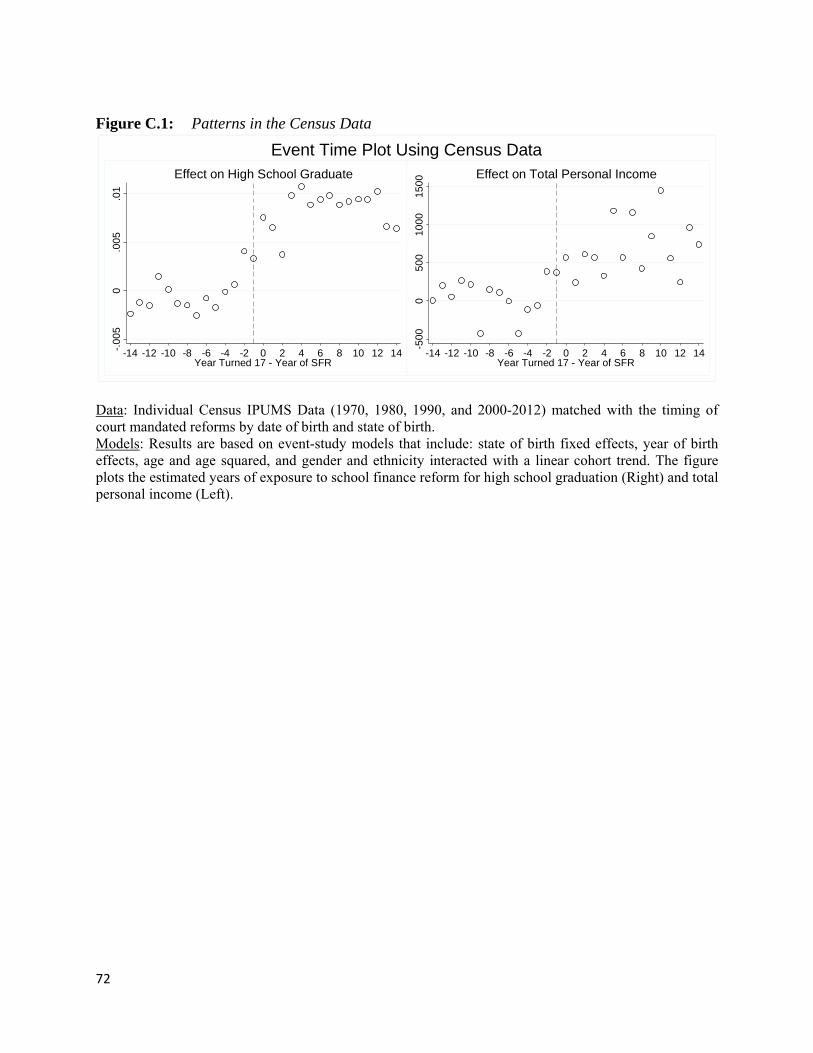
72  

Figure C.1: Patterns in the Census Data

Data: Individual Census IPUMS Data (1970, 1980, 1990, and 2000-2012) matched with the timing of court mandated reforms by date of birth and state of birth. Models: Results are based on event-study models that include: state of birth fixed effects, year of birth effects, age and age squared, and gender and ethnicity interacted with a linear cohort trend. The figure plots the estimated years of exposure to school finance reform for high school graduation (Right) and total personal income (Left).

-50

00

50

01

00

01

50

0

-14 -12 -10 -8 -6 -4 -2 0 2 4 6 8 10 12 14Year Turned 17 - Year of SFR

Effect on Total Personal Income

-.0

05

0.0

05

.01

-14 -12 -10 -8 -6 -4 -2 0 2 4 6 8 10 12 14Year Turned 17 - Year of SFR

Effect on High School Graduate

Event Time Plot Using Census Data

73  

Appendix D: Data Sources for Part 1 Per Pupil Spending Data

Previous historical data on per pupil expenditures was only available in a readily usable format via the Census of Governments: School System Finance (F-33) File (U.S. Bureau of the Census, Department of Commerce). The Census of Governments previously was only conducted in years that end in a two or seven, so at the time when many important papers on SFRs were written, there were many years of missing data. In addition, until recently the earliest available F-33 data was for the year 1972. As a result, it was previously impossible to model per pupil spending and spending inequality annually over time, so many authors (e.g., MES, Card and Payne), operating under the Common Trends Assumption, assumed that trends in per pupil spending were linear. Due to these limitations, previous papers on school finance reforms were also unable to look at how the exact timing of reforms affected per pupil expenditure and spending inequality within a state.

Our data from the Historical Database on Individual Government Finances (INDFIN) represents the Census Bureau’s first effort to provide a time series of historically consistent data on the finances of individual governments. This database combines data from the Census of Governments Survey of Government Finances (F-33), the National Archives, and the Individual Government Finances Survey. The School District Finance Data FY 1967-91 is available annually from 1967 through 1991. It contains over one million individual local government records, including counties, cities, townships, special districts, and independent school districts. The INDFIN database frees the researcher from the arduous task of reconciling the many technical, classification, and other data-related changes that have occurred over the last 30 years. For example, this database includes corrected statistical weights that have been standardized across years, which had not been done previously. Furthermore, although most governments retain the ID number they are assigned originally, there are circumstances that result in a government's ID being changed. Since a major purpose of the INDFIN database is tracking government finances over time, it is critical that a government possess the same ID for all years (unless the ID change had a major structural cause). For example, All Alaska IDs were changed in the 1982 Census of Governments. In addition, new county incorporations, where governments in the new county area are re-assigned an ID based on the new county code (e.g., La Paz County, AZ), cause ID changes. Thus, if a government ID number was changed, the ID used in the database is its current GID number, including those preceding the cause of the change, so that the ID is standardized across years.

In addition to standardizing the data, the Census Bureau has corrected a number of errors in the INDFIN database that were previously in other sources of data. For example, for fiscal years 1974, 1975, 1976 and 1978 the school district enrollment data that had previously been released were useless (either missing or in error for many records). Thus, in August 2000, these missing enrollment data were replaced with those from the employment survey individual unit files. This enables us to more accurately compute per pupil expenditures for those years. In addition, source files before fiscal 1977 were in whole dollars rather than thousands. This set a limit on the largest value any field could hold. If a figure exceeded that amount, then the field contained a special "overflow" flag (999999999). Few governments exceeded the limit (Port Authority of NY and NJ and Los Angeles County, CA are two that did). For the INDFIN database, actual data were substituted for the overflow flag. Finally, in some cases the Census revised the original data in source files for the INDFIN database. In some cases, official

74  

revisions were never applied to the data files. Others resulted from the different environment and operating practices under which source files were created. Finally, some extreme outliers were identified and corrected (e.g., a keying error for a small government that ballooned its data).

The Common Core of Data (CCD) School District Finance Survey (F-33) consists of data submitted annually to the National Center for Education Statistics (NCES) by state education agencies (SEAs) in the 50 states and the District of Columbia. The purpose of the survey is to provide finance data for all local education agencies (LEAs) that provide free public elementary and secondary education in the United States. Both NCES and the Governments Division of the U.S. Census Bureau collect public school system finance data, and they collaborate in their efforts to gather these data. The Census of Governments, which was recorded every five years until 1992, records administrative data on school spending for every district in the United States. After 1992, the Public Elementary-Secondary Education Finances data were recorded annually with data available until 2010. We combine these data sources to construct a long panel of annual per pupil spending for each school district in the United States between 1967 and 2010.

Per-pupil spending data from before 1992 is missing for Alaska, Hawaii, Maryland, North Carolina, Virginia, and Washington, D.C. Per-pupil spending data from 1968 and 1969 is missing for all states. Spending data in Florida was also missing for 1975, 1983, 1985-1987, and 1991. Spending data in Kansas was also missing for 1977 and 1986. Spending data in Mississippi was also missing for 1985 and 1988. Spending data in Wyoming was also missing for 1979 and 1984. Spending data for Montana is missing in 1976, data for Nebraska is missing in 1977, and data for Texas is missing in 1991. Where there was only a year or two of missing per pupil expenditure data, we filled in this data using linear interpolation.

Data on School Finance Reforms

Due to great interest on the topic, the timing of school finance reforms (SFRs) has been collected in various places. Data on the exact timing and type of court ordered and legislative SFRs was obtained from Public School Finance Programs of the Unites States and Canada (PSFP), National Access Network’s state by state school finance litigation map (2011), from Murray, Evans, and Schwab (1998), Hoxby (2001), Card and Payne (2002), Hightower et al (2010), and Baicker and Gordon (2004). The most accurate information on school finance laws can be derived from the PSFP, which provides basic information and references to the legislation and court cases challenging them (Hoxby, 2001). In most cases, data from these sources are consistent with each other. Where there are discrepancies we often defer to PSFP, but also consulted LexisNexis and state court and legislation records.

There were discrepancies in reported timing of overturned court cases in several states: Connecticut (Hoxby states the decision was made in 1978, but Card and Payne report it was made in 1977), Kansas (Hoxby states 1976, but PSFP and ACCESS report 1972), New Jersey (Card and Payne state 1989, but PSFP says 1990), Washington (Murray, Evans, and Schwab, Hoxby, and Card and Payne report 1978, but PSFP reports 1977), Wyoming (Hoxby says 1983, but Card and Payne and Murray, Evans, and Schwab report 1980). We researched each case by name to discover the true date of the decision.

Using a policy survey conducted during the 2008-2009 school year, a recent study by Hightower et al (2010) provides a description of state finance policies and practices. This study was used to verify whether there had been any changes to state funding formulas between 1998 and 2009. We only collected information on the first five court cases per state in which the state

75  

found the school funding system unconstitutional. There were only three states with five or more court cases overruling the funding system (New Hampshire, New Jersey, and Texas). In addition, we only collected information on the first four court cases per state in which states upheld the school funding system. There were only four states with four or more court cases in which the school funding system was upheld (Illinois, New York, Oregon, and Pennsylvania).

Information on whether or not a state funding formula had a MFP, flat grant formula, variable matching grant scheme, recapture provision, spending limit, power equalization scheme, local-effort equalization scheme, or full state funding came from PSFP (1998) and was verified using Card and Payne (2002) and Hightower et al (2010). We defined MFPs, flat grant formulas, and variable matching grant schemes in the same way as Card and Payne did in their 2002 study. We defined power equalization, local-effort equalization, and full state funding in the same way as the EPE study (Hightower, Mitani and Swanson, 2010). Each element of a state funding formula was coded as a dichotomous variable. For example, MFP is a dichotomous variable that is equal to one in the year and all subsequent years in which a state’s finance system had a MFP plan in place. MFP was set equal to zero in all years prior to the state’s funding system having a MFP in place, or if a state never implemented a MFP. Information on adequacy and equity reforms came from Berry (2005) and Springer, Liu and Guthrie (2009)’s Table 1. Following Springer, Lui and Guthrie (2009), we define two dichotomous variables for equity and adequacy reforms. Adequacy is a dichotomous variable set to one in the year, and all subsequent years, in which a state’s finance system was overturned on adequacy grounds. Adequacy is set to zero in all years prior to a school funding mechanism being overturned, or if a state’s finance system was never ruled unconstitutional. Similarly, equity is a dichotomous variable that is set to one in the year, and in all subsequent years, in which a state’s finance system was ruled unconstitutional on equity grounds. Equity was set to zero in all years prior to the state funding mechanism being declared unconstitutional, or if a state’s funding mechanism was never overturned.

Information on the timing of tax limits came from Downes and Figlio (1998). In addition, information on the foundation property tax rate and the maximum/minimum inverted tax price of marginal local spending was obtained from Hoxby (2001) and defined in the same way. Thus, we defined a variable, limit2, which equals one if there is a zero tax price according to Hoxby, a recapture provision, or a spending cap. We defined another variable, g1taxprice, as equal to one if the inverted tax price was greater than one (which should promote spending).

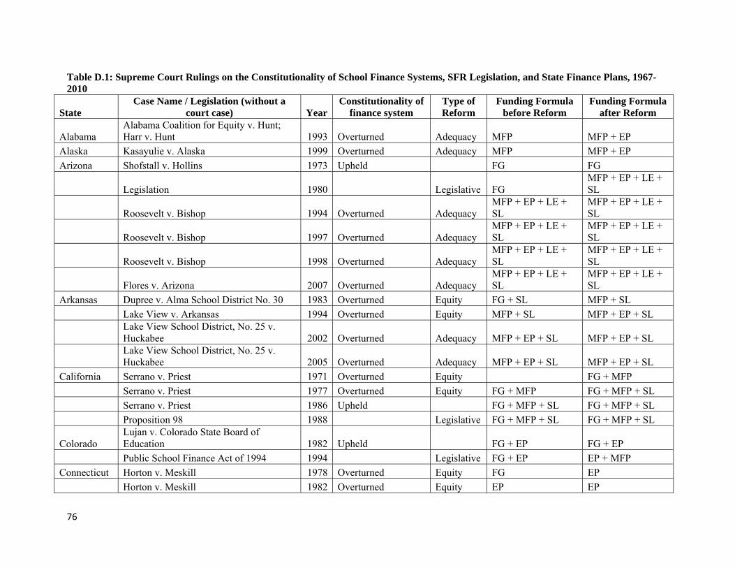
76  

Table D.1: Supreme Court Rulings on the Constitutionality of School Finance Systems, SFR Legislation, and State Finance Plans, 1967-2010

State Case Name / Legislation (without a

court case) YearConstitutionality of

finance system Type of Reform

Funding Formula before Reform

Funding Formula after Reform

Alabama Alabama Coalition for Equity v. Hunt; Harr v. Hunt 1993 Overturned Adequacy MFP MFP + EP

Alaska Kasayulie v. Alaska 1999 Overturned Adequacy MFP MFP + EP Arizona Shofstall v. Hollins 1973 Upheld FG FG

Legislation 1980 Legislative FG MFP + EP + LE + SL

Roosevelt v. Bishop 1994 Overturned Adequacy MFP + EP + LE + SL

MFP + EP + LE + SL

Roosevelt v. Bishop 1997 Overturned Adequacy MFP + EP + LE + SL

MFP + EP + LE + SL

Roosevelt v. Bishop 1998 Overturned Adequacy MFP + EP + LE + SL

MFP + EP + LE + SL

Flores v. Arizona 2007 Overturned Adequacy MFP + EP + LE + SL

MFP + EP + LE + SL

Arkansas Dupree v. Alma School District No. 30 1983 Overturned Equity FG + SL MFP + SL Lake View v. Arkansas 1994 Overturned Equity MFP + SL MFP + EP + SL Lake View School District, No. 25 v. Huckabee 2002 Overturned Adequacy MFP + EP + SL MFP + EP + SL Lake View School District, No. 25 v. Huckabee 2005 Overturned Adequacy MFP + EP + SL MFP + EP + SL

California Serrano v. Priest 1971 Overturned Equity FG + MFP Serrano v. Priest 1977 Overturned Equity FG + MFP FG + MFP + SL Serrano v. Priest 1986 Upheld FG + MFP + SL FG + MFP + SL Proposition 98 1988 Legislative FG + MFP + SL FG + MFP + SL

Colorado Lujan v. Colorado State Board of Education 1982 Upheld FG + EP FG + EP Public School Finance Act of 1994 1994 Legislative FG + EP EP + MFP

Connecticut Horton v. Meskill 1978 Overturned Equity FG EP Horton v. Meskill 1982 Overturned Equity EP EP

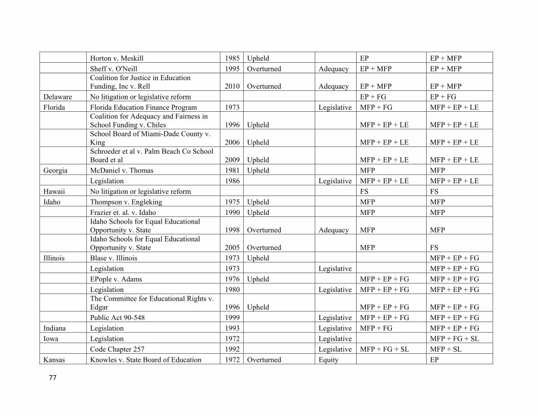
77  

Horton v. Meskill 1985 Upheld EP EP + MFP Sheff v. O'Neill 1995 Overturned Adequacy EP + MFP EP + MFP Coalition for Justice in Education Funding, Inc v. Rell 2010 Overturned Adequacy EP + MFP EP + MFP

Delaware No litigation or legislative reform EP + FG EP + FG Florida Florida Education Finance Program 1973 Legislative MFP + FG MFP + EP + LE

Coalition for Adequacy and Fairness in School Funding v. Chiles 1996 Upheld MFP + EP + LE MFP + EP + LE School Board of Miami-Dade County v. King 2006 Upheld MFP + EP + LE MFP + EP + LE Schroeder et al v. Palm Beach Co School Board et al 2009 Upheld MFP + EP + LE MFP + EP + LE

Georgia McDaniel v. Thomas 1981 Upheld MFP MFP Legislation 1986 Legislative MFP + EP + LE MFP + EP + LE

Hawaii No litigation or legislative reform FS FS Idaho Thompson v. Engleking 1975 Upheld MFP MFP

Frazier et. al. v. Idaho 1990 Upheld MFP MFP Idaho Schools for Equal Educational Opportunity v. State 1998 Overturned Adequacy MFP MFP Idaho Schools for Equal Educational Opportunity v. State 2005 Overturned MFP FS

Illinois Blase v. Illinois 1973 Upheld MFP + EP + FG Legislation 1973 Legislative MFP + EP + FG EPople v. Adams 1976 Upheld MFP + EP + FG MFP + EP + FG Legislation 1980 Legislative MFP + EP + FG MFP + EP + FG The Committee for Educational Rights v. Edgar 1996 Upheld MFP + EP + FG MFP + EP + FG Public Act 90-548 1999 Legislative MFP + EP + FG MFP + EP + FG

Indiana Legislation 1993 Legislative MFP + FG MFP + EP + FG Iowa Legislation 1972 Legislative MFP + FG + SL

Code Chapter 257 1992 Legislative MFP + FG + SL MFP + SL Kansas Knowles v. State Board of Education 1972 Overturned Equity EP

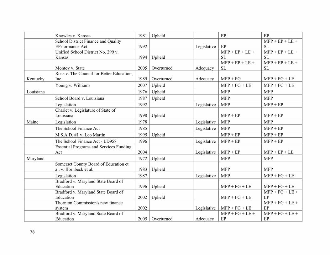
78  

Knowles v. Kansas 1981 Upheld EP EP School District Finance and Quality EPrformance Act 1992 Legislative EP

MFP + EP + LE + SL

Unified School District No. 299 v. Kansas 1994 Upheld

MFP + EP + LE + SL

MFP + EP + LE + SL

Montoy v. State 2005 Overturned Adequacy MFP + EP + LE + SL

MFP + EP + LE + SL

Kentucky Rose v. The Council for Better Education, Inc. 1989 Overturned Adequacy MFP + FG MFP + FG + LE Young v. Williams 2007 Upheld MFP + FG + LE MFP + FG + LE

Louisiana 1976 Upheld MFP MFP School Board v. Louisiana 1987 Upheld MFP MFP Legislation 1992 Legislative MFP MFP + EP Charlet v. Legislature of State of Louisiana 1998 Upheld MFP + EP MFP + EP

Maine Legislation 1978 Legislative MFP MFP The School Finance Act 1985 Legislative MFP MFP + EP M.S.A.D. #1 v. Leo Martin 1995 Upheld MFP + EP MFP + EP The School Finance Act - LD958 1996 Legislative MFP + EP MFP + EP Essential Programs and Services Funding Act 2004 Legislative MFP + EP MFP + EP + LE

Maryland 1972 Upheld MFP MFP Somerset County Board of Education et al. v. fIornbeck et al. 1983 Upheld MFP MFP Legislation 1987 Legislative MFP MFP + FG + LE Bradford v. Maryland State Board of Education 1996 Upheld MFP + FG + LE MFP + FG + LE Bradford v. Maryland State Board of Education 2002 Upheld MFP + FG + LE

MFP + FG + LE + EP

Thornton Commission's new finance system 2002 Legislative MFP + FG + LE

MFP + FG + LE + EP

Bradford v. Maryland State Board of Education 2005 Overturned Adequacy

MFP + FG + LE + EP

MFP + FG + LE + EP

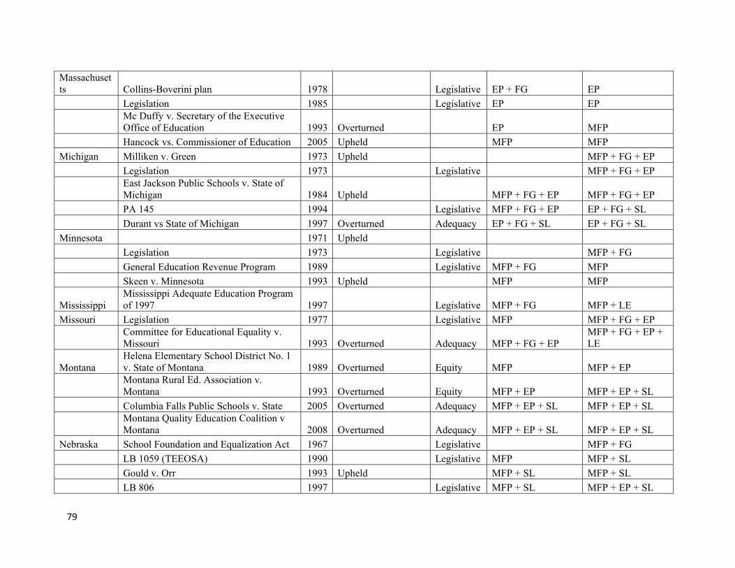
79  

Massachusetts Collins-Boverini plan 1978 Legislative EP + FG EP

Legislation 1985 Legislative EP EP Mc Duffy v. Secretary of the Executive Office of Education 1993 Overturned EP MFP Hancock vs. Commissioner of Education 2005 Upheld MFP MFP

Michigan Milliken v. Green 1973 Upheld MFP + FG + EP Legislation 1973 Legislative MFP + FG + EP East Jackson Public Schools v. State of Michigan 1984 Upheld MFP + FG + EP MFP + FG + EP PA 145 1994 Legislative MFP + FG + EP EP + FG + SL Durant vs State of Michigan 1997 Overturned Adequacy EP + FG + SL EP + FG + SL

Minnesota 1971 Upheld Legislation 1973 Legislative MFP + FG General Education Revenue Program 1989 Legislative MFP + FG MFP Skeen v. Minnesota 1993 Upheld MFP MFP

Mississippi Mississippi Adequate Education Program of 1997 1997 Legislative MFP + FG MFP + LE

Missouri Legislation 1977 Legislative MFP MFP + FG + EP Committee for Educational Equality v. Missouri 1993 Overturned Adequacy MFP + FG + EP

MFP + FG + EP + LE

Montana Helena Elementary School District No. 1 v. State of Montana 1989 Overturned Equity MFP MFP + EP Montana Rural Ed. Association v. Montana 1993 Overturned Equity MFP + EP MFP + EP + SL Columbia Falls Public Schools v. State 2005 Overturned Adequacy MFP + EP + SL MFP + EP + SL Montana Quality Education Coalition v Montana 2008 Overturned Adequacy MFP + EP + SL MFP + EP + SL

Nebraska School Foundation and Equalization Act 1967 Legislative MFP + FG LB 1059 (TEEOSA) 1990 Legislative MFP MFP + SL Gould v. Orr 1993 Upheld MFP + SL MFP + SL LB 806 1997 Legislative MFP + SL MFP + EP + SL

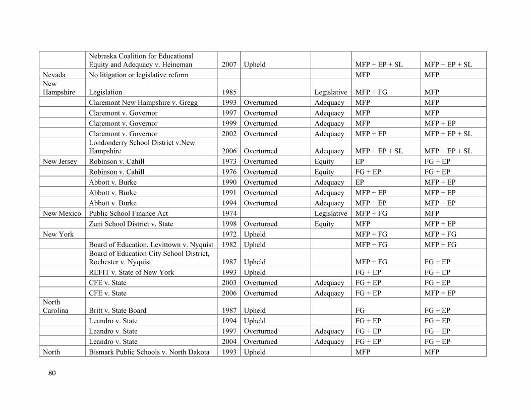
80  

Nebraska Coalition for Educational Equity and Adequacy v. Heineman 2007 Upheld MFP + EP + SL MFP + EP + SL

Nevada No litigation or legislative reform MFP MFP New Hampshire Legislation 1985 Legislative MFP + FG MFP

Claremont New Hampshire v. Gregg 1993 Overturned Adequacy MFP MFP Claremont v. Governor 1997 Overturned Adequacy MFP MFP Claremont v. Governor 1999 Overturned Adequacy MFP MFP + EP Claremont v. Governor 2002 Overturned Adequacy MFP + EP MFP + EP + SL Londonderry School District v.New Hampshire 2006 Overturned Adequacy MFP + EP + SL MFP + EP + SL

New Jersey Robinson v. Cahill 1973 Overturned Equity EP FG + EP Robinson v. Cahill 1976 Overturned Equity FG + EP FG + EP Abbott v. Burke 1990 Overturned Adequacy EP MFP + EP Abbott v. Burke 1991 Overturned Adequacy MFP + EP MFP + EP Abbott v. Burke 1994 Overturned Adequacy MFP + EP MFP + EP

New Mexico Public School Finance Act 1974 Legislative MFP + FG MFP Zuni School District v. State 1998 Overturned Equity MFP MFP + EP

New York 1972 Upheld MFP + FG MFP + FG Board of Education, Levittown v. Nyquist 1982 Upheld MFP + FG MFP + FG Board of Education City School District, Rochester v. Nyquist 1987 Upheld MFP + FG FG + EP REFIT v. State of New York 1993 Upheld FG + EP FG + EP CFE v. State 2003 Overturned Adequacy FG + EP FG + EP CFE v. State 2006 Overturned Adequacy FG + EP MFP + EP

North Carolina Britt v. State Board 1987 Upheld FG FG + EP

Leandro v. State 1994 Upheld FG + EP FG + EP Leandro v. State 1997 Overturned Adequacy FG + EP FG + EP Leandro v. State 2004 Overturned Adequacy FG + EP FG + EP

North Bismark Public Schools v. North Dakota 1993 Upheld MFP MFP

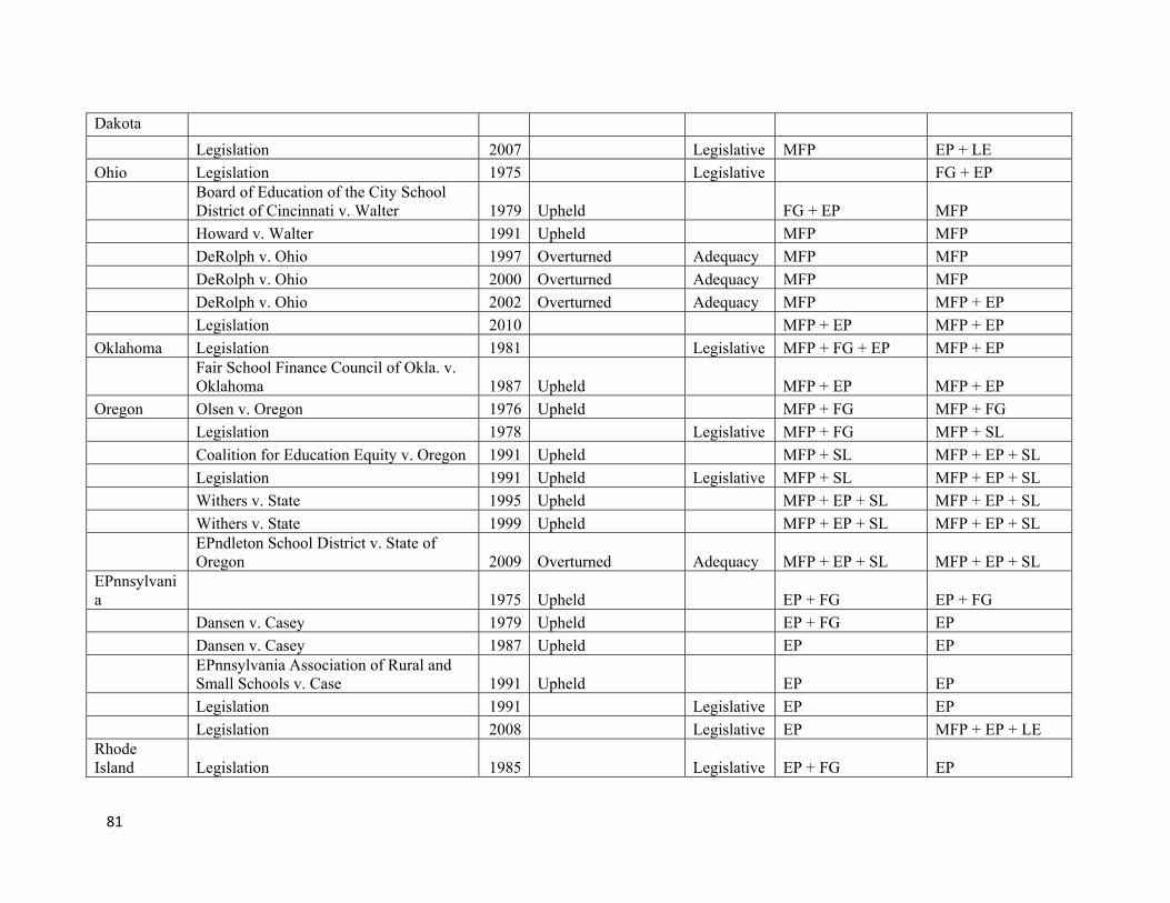
81  

Dakota Legislation 2007 Legislative MFP EP + LE

Ohio Legislation 1975 Legislative FG + EP Board of Education of the City School District of Cincinnati v. Walter 1979 Upheld FG + EP MFP Howard v. Walter 1991 Upheld MFP MFP DeRolph v. Ohio 1997 Overturned Adequacy MFP MFP DeRolph v. Ohio 2000 Overturned Adequacy MFP MFP DeRolph v. Ohio 2002 Overturned Adequacy MFP MFP + EP Legislation 2010 MFP + EP MFP + EP

Oklahoma Legislation 1981 Legislative MFP + FG + EP MFP + EP Fair School Finance Council of Okla. v. Oklahoma 1987 Upheld MFP + EP MFP + EP

Oregon Olsen v. Oregon 1976 Upheld MFP + FG MFP + FG Legislation 1978 Legislative MFP + FG MFP + SL Coalition for Education Equity v. Oregon 1991 Upheld MFP + SL MFP + EP + SL Legislation 1991 Upheld Legislative MFP + SL MFP + EP + SL Withers v. State 1995 Upheld MFP + EP + SL MFP + EP + SL Withers v. State 1999 Upheld MFP + EP + SL MFP + EP + SL EPndleton School District v. State of Oregon 2009 Overturned Adequacy MFP + EP + SL MFP + EP + SL

EPnnsylvania 1975 Upheld EP + FG EP + FG

Dansen v. Casey 1979 Upheld EP + FG EP Dansen v. Casey 1987 Upheld EP EP EPnnsylvania Association of Rural and Small Schools v. Case 1991 Upheld EP EP Legislation 1991 Legislative EP EP Legislation 2008 Legislative EP MFP + EP + LE

Rhode Island Legislation 1985 Legislative EP + FG EP

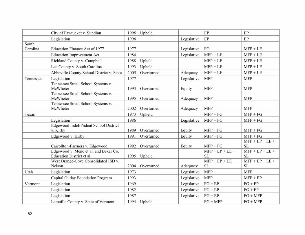
82  

City of Pawtucket v. Sundlun 1995 Upheld EP EP Legislation 1996 Legislative EP EP

South Carolina Education Finance Act of 1977 1977 Legislative FG MFP + LE

Education Improvement Act 1984 Legislative MFP + LE MFP + LE Richland County v. Campbell 1988 Upheld MFP + LE MFP + LE Lee County v. South Carolina 1993 Upheld MFP + LE MFP + LE Abbeville County School District v. State 2005 Overturned Adequacy MFP + LE MFP + LE

Tennessee Legislation 1977 Legislative MFP MFP Tennessee Small School Systems v. McWheter 1993 Overturned Equity MFP MFP Tennessee Small School Systems v. McWheter 1995 Overturned Adequacy MFP MFP Tennessee Small School Systems v. McWheter 2002 Overturned Adequacy MFP MFP

Texas 1973 Upheld MFP + FG MFP + FG Legislation 1986 Legislative MFP + FG MFP + FG Edgewood IndeEPndent School District v. Kirby 1989 Overturned Equity MFP + FG MFP + FG Edgewood v. Kirby 1991 Overturned Equity MFP + FG MFP + FG

Carrollton-Farrners v. Edgewood 1992 Overturned Equity MFP + FG MFP + EP + LE + SL

Edgewood v. Meno et al. and Bexar Co. Education District et al. 1995 Upheld

MFP + EP + LE + SL

MFP + EP + LE + SL

West Orange-Cove Consolidated ISD v. Nelson 2004 Overturned Adequacy

MFP + EP + LE + SL

MFP + EP + LE + SL

Utah Legislation 1973 Legislative MFP MFP Capital Outlay Foundation Program 1993 Legislative MFP MFP + EP

Vermont Legislation 1969 Legislative FG + EP FG + EP Legislation 1982 Legislative FG + EP FG + EP Legislation 1987 Legislative FG + EP FG + MFP Lamoille County v. State of Vermont 1994 Upheld FG + MFP FG + MFP

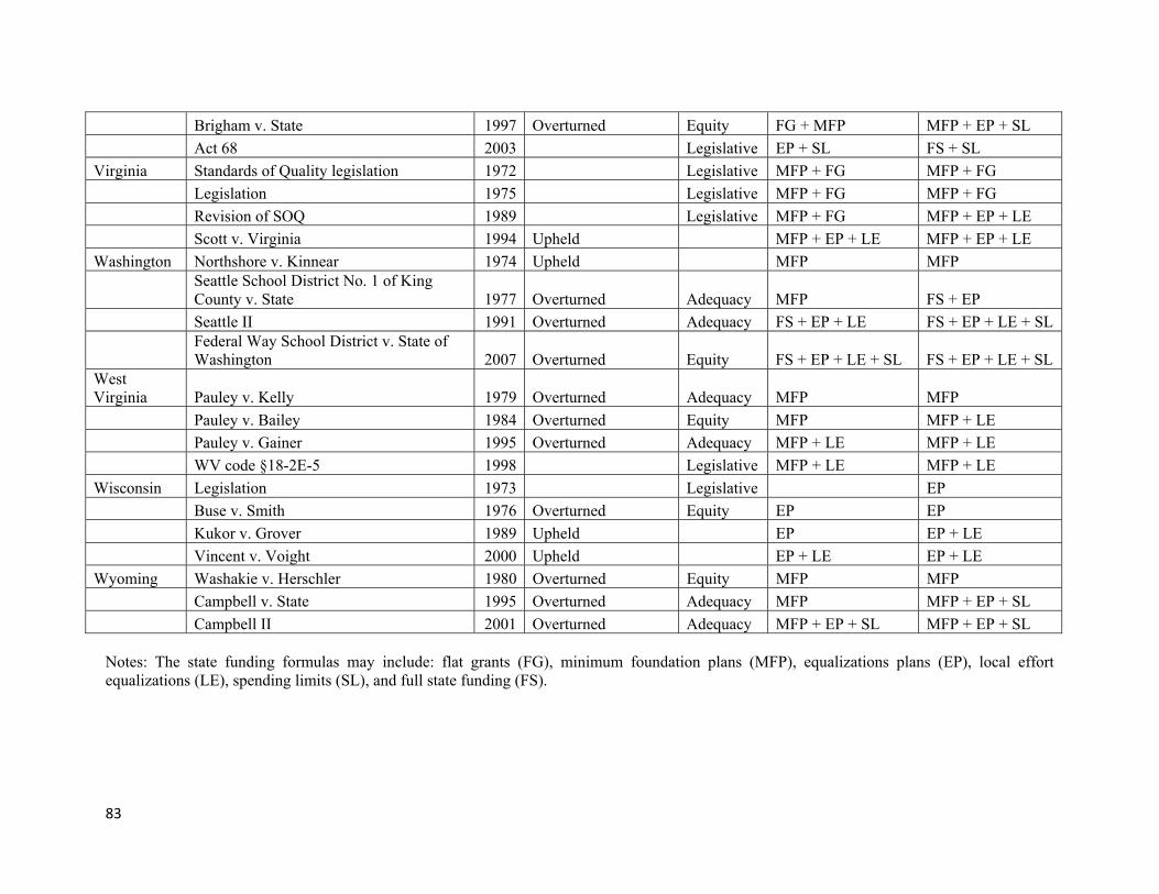
83  

Brigham v. State 1997 Overturned Equity FG + MFP MFP + EP + SL Act 68 2003 Legislative EP + SL FS + SL

Virginia Standards of Quality legislation 1972 Legislative MFP + FG MFP + FG Legislation 1975 Legislative MFP + FG MFP + FG Revision of SOQ 1989 Legislative MFP + FG MFP + EP + LE Scott v. Virginia 1994 Upheld MFP + EP + LE MFP + EP + LE

Washington Northshore v. Kinnear 1974 Upheld MFP MFP Seattle School District No. 1 of King County v. State 1977 Overturned Adequacy MFP FS + EP Seattle II 1991 Overturned Adequacy FS + EP + LE FS + EP + LE + SL Federal Way School District v. State of Washington 2007 Overturned Equity FS + EP + LE + SL FS + EP + LE + SL

West Virginia Pauley v. Kelly 1979 Overturned Adequacy MFP MFP

Pauley v. Bailey 1984 Overturned Equity MFP MFP + LE Pauley v. Gainer 1995 Overturned Adequacy MFP + LE MFP + LE WV code §18-2E-5 1998 Legislative MFP + LE MFP + LE

Wisconsin Legislation 1973 Legislative EP Buse v. Smith 1976 Overturned Equity EP EP Kukor v. Grover 1989 Upheld EP EP + LE Vincent v. Voight 2000 Upheld EP + LE EP + LE

Wyoming Washakie v. Herschler 1980 Overturned Equity MFP MFP Campbell v. State 1995 Overturned Adequacy MFP MFP + EP + SL Campbell II 2001 Overturned Adequacy MFP + EP + SL MFP + EP + SL

Notes: The state funding formulas may include: flat grants (FG), minimum foundation plans (MFP), equalizations plans (EP), local effort equalizations (LE), spending limits (SL), and full state funding (FS).

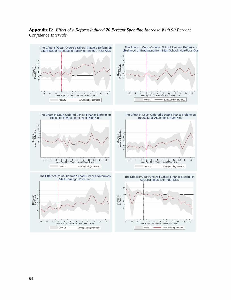
84  

Appendix E: Effect of a Reform Induced 20 Percent Spending Increase With 90 Percent Confidence Intervals

-.1

0

.1

.2

.3

.4

Cha

nge

inP

rob(

HS

Gra

d)

-6 -4 -2 0 2 4 6 8 10 12 14 16Year Aged 17 - Year of Initial Court Order

90% CI 20%spending increase

The Effect of Court-Ordered School Finance Reform onLikelihood of Graduating from High School, Poor Kids

-.1

0

.1

.2

.3

.4

Cha

nge

inP

rob(

HS

Gra

d)

-6 -4 -2 0 2 4 6 8 10 12 14 16Year Aged 17 - Year of Initial Court Order

90% CI 20%spending increase

The Effect of Court-Ordered School Finance Reform onLikelihood of Graduating from High School, Non-Poor Kids

0

.5

1

1.5

2

Cha

nge

inY

ear

s of

Ed

uca

tion

-6 -4 -2 0 2 4 6 8 10 12 14 16Year Aged 17 - Year of Initial Court Order

90% CI 20%spending increase

The Effect of Court-Ordered School Finance Reform onEducational Attainment, Non-Poor Kids

0

.5

1

1.5

2

Cha

nge

inY

ear

s of

Ed

uca

tion

-6 -4 -2 0 2 4 6 8 10 12 14 16Year Aged 17 - Year of Initial Court Order

90% CI 20%spending increase

The Effect of Court-Ordered School Finance Reform onEducational Attainment, Poor Kids

0

.2

.4

.6

.8

1

Cha

nge

inL

n(W

age)

-6 -4 -2 0 2 4 6 8 10 12 14 16Year Aged 17 - Year of Initial Court Order

90% CI 20%spending increase

The Effect of Court-Ordered School Finance Reform onAdult Earnings, Poor Kids

-1

-.5

0

.5

Cha

nge

inL

n(W

age)

-6 -4 -2 0 2 4 6 8 10 12 14 16Year Aged 17 - Year of Initial Court Order

90% CI 20%spending increase

The Effect of Court-Ordered School Finance Reform onAdult Earnings, Non-Poor Kids

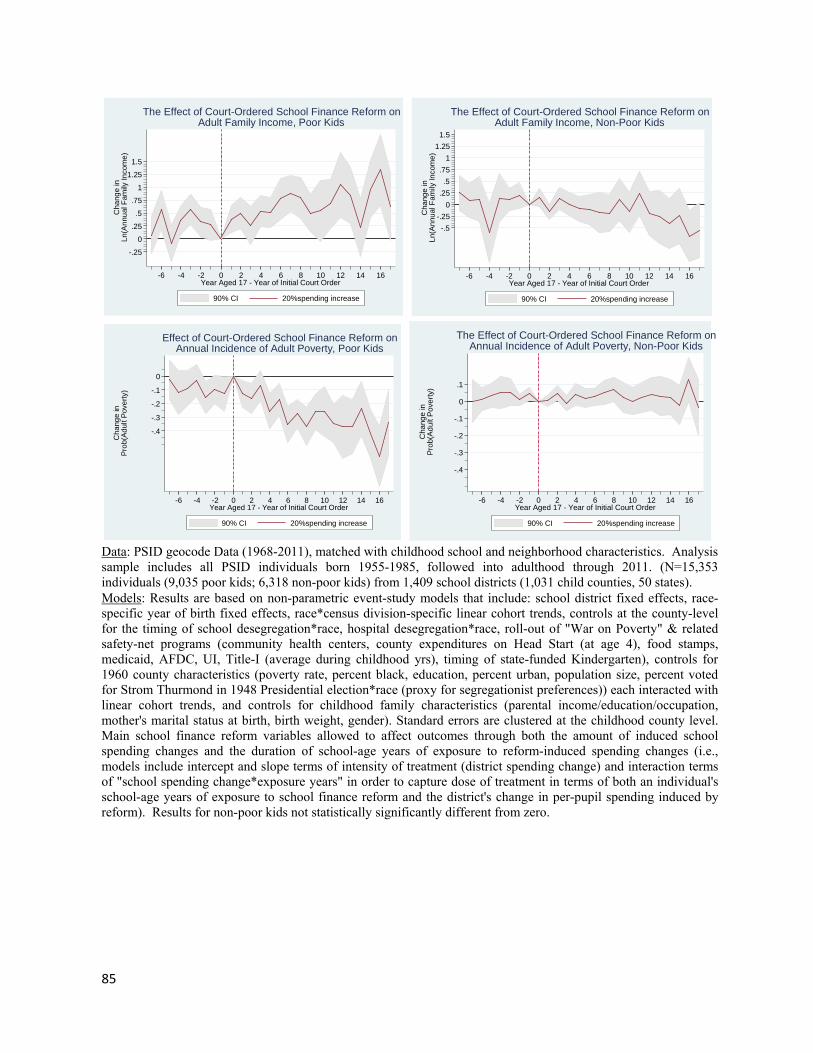
85  

Data: PSID geocode Data (1968-2011), matched with childhood school and neighborhood characteristics. Analysis sample includes all PSID individuals born 1955-1985, followed into adulthood through 2011. (N=15,353 individuals (9,035 poor kids; 6,318 non-poor kids) from 1,409 school districts (1,031 child counties, 50 states). Models: Results are based on non-parametric event-study models that include: school district fixed effects, race-specific year of birth fixed effects, race*census division-specific linear cohort trends, controls at the county-level for the timing of school desegregation*race, hospital desegregation*race, roll-out of "War on Poverty" & related safety-net programs (community health centers, county expenditures on Head Start (at age 4), food stamps, medicaid, AFDC, UI, Title-I (average during childhood yrs), timing of state-funded Kindergarten), controls for 1960 county characteristics (poverty rate, percent black, education, percent urban, population size, percent voted for Strom Thurmond in 1948 Presidential election*race (proxy for segregationist preferences)) each interacted with linear cohort trends, and controls for childhood family characteristics (parental income/education/occupation, mother's marital status at birth, birth weight, gender). Standard errors are clustered at the childhood county level. Main school finance reform variables allowed to affect outcomes through both the amount of induced school spending changes and the duration of school-age years of exposure to reform-induced spending changes (i.e., models include intercept and slope terms of intensity of treatment (district spending change) and interaction terms of "school spending change*exposure years" in order to capture dose of treatment in terms of both an individual's school-age years of exposure to school finance reform and the district's change in per-pupil spending induced by reform). Results for non-poor kids not statistically significantly different from zero.

-.25

0

.25

.5

.75

1

1.25

1.5

Cha

nge

inL

n(A

nnu

al F

amily

Inco

me

)

-6 -4 -2 0 2 4 6 8 10 12 14 16Year Aged 17 - Year of Initial Court Order

90% CI 20%spending increase

The Effect of Court-Ordered School Finance Reform onAdult Family Income, Poor Kids

-.5

-.25

0

.25

.5

.75

1

1.25

1.5

Cha

nge

inL

n(A

nnu

al F

amily

Inco

me

)

-6 -4 -2 0 2 4 6 8 10 12 14 16Year Aged 17 - Year of Initial Court Order

90% CI 20%spending increase

The Effect of Court-Ordered School Finance Reform onAdult Family Income, Non-Poor Kids

-.4

-.3

-.2

-.1

0

Cha

nge

inP

rob(

Ad

ult P

ove

rty)

-6 -4 -2 0 2 4 6 8 10 12 14 16Year Aged 17 - Year of Initial Court Order

90% CI 20%spending increase

Effect of Court-Ordered School Finance Reform onAnnual Incidence of Adult Poverty, Poor Kids

-.4

-.3

-.2

-.1

0

.1

Cha

nge

inP

rob(

Ad

ult P

ove

rty)

-6 -4 -2 0 2 4 6 8 10 12 14 16Year Aged 17 - Year of Initial Court Order

90% CI 20%spending increase

The Effect of Court-Ordered School Finance Reform onAnnual Incidence of Adult Poverty, Non-Poor Kids