Behavioral finance:

The January effect

Bachelor Thesis: Finance Tilburg University 06-07-2012

Tijmen Kampman 659219

Supervisor: P. F. A. Tuijp

2

Abstract

The January effect is a thoroughly and well researched anomaly in the academic financial

world. However, even after all this research a definite explanation for this effect has not been

given yet. The explanation that has gotten the most attention from the most cited papers is the

tax-loss selling effect. This explanation states that investors sell their losing stock at the end

of the year, thus generating a loss so they can reduce the amount of tax they have to pay at the

end of the fiscal year. After the tax-loss selling hypothesis some other possible explanations

for the January effect are discussed together with a review of the Other January effect.

Furthermore, an empirical research is conducted using index data from the Standards and

Poor’s 500 (S&P 500) between 1975 and 2000. This thesis does not find significant evidence

for the existence of the January effect at a 0.05 probability level. There is some indication that

January is a good indicator for the rest of the year in the literate, but the empirical results are

not significant for this to be concluded.

3

Table of Contents

Abstract ............................................................................................................................................... 2

1. Introduction and Problem formulation ........................................................................................ 4

1.1 Introduction ......................................................................................................................... 4

2. Literature Review ........................................................................................................................ 6

2.1 Efficient Market Hypothesis ................................................................................................ 6

2.2 The January effect ............................................................................................................... 7

2.3 The tax-loss selling explanation .......................................................................................... 8

2.4 Others explanations ............................................................................................................. 9

2.5 The Other January effect ................................................................................................... 10

2.6 Data snooping .................................................................................................................... 11

3. Data and methodology ................................................................................................................... 13

4. Empirical Results .......................................................................................................................... 14

4.1 The January effect ................................................................................................................... 14

4.2 The Other January effect ......................................................................................................... 17

5. Conclusion ..................................................................................................................................... 19

5.1 Conclusions & limitations ....................................................................................................... 19

5.2 Recommendations for future research ..................................................................................... 21

References: ........................................................................................................................................ 22

4

1. Introduction and Problem formulation

1.1 Introduction

The topic for this bachelor thesis is the January effect. This effect is an anomaly found in the

month January. Stocks, and especially small stocks, tend to perform very well in January

compared to the other months. Wachtel (1942) is generally seen as the first researcher that

found the January effect. After his discovery, Rozeff and Kinney (1976) were one of the first

that investigated this particular pattern. To be more precise, Rozeff and Kinney (1976) found

seasonal patterns in an equal-weighted index of the New York Stock Exchange prices over the

period 1904-74. In their study they established that the average monthly return in January was

3.5 percent. In other months this was only 0.5 percent. Another important finding was that this

effect was not observed in an index that was only composed of large firms.

After Rozeff and Kinney made this first step in exploring this phenomenon, others quickly

followed in their footsteps. In a study performed by Banz (1981), evidence was found that

small firms earn higher returns than the expected returns. Keim (1983) investigated whether

the excess returns of small firms were temporally concentrated. He found that half of the

returns in January came from the first five trading days. Over the years researchers have come

with up answers to why this January effect occurs. Reinganum (1983) investigated a possible

explanation of the January effect based on tax-loss selling. The idea is that firms will sell their

losing shares at the end of the year, this way trying to realize some capital losses. While the

evidence found by the researchers suggest that taxes have something to do with the January

effect, it cannot be the entire explanation. Kato and Schallheim (1985) also found a January

effect in Japan. Because there are no capital gains/loss tax offsets in Japan, there has to be

another explanation for the higher returns in January. Japan is not the only example where the

tax argument doesn’t hold up. In countries like Canada, Australia and Great Britain

researchers also found a January effect, but their tax years start at respectively 1 April and 1

July. Gultekin and Gultekin (1983) found more international evidence to support the January

effect.

Another interesting idea found by De Bondt and Thaler (1985) is that firms who have been

big winners or losers in the last five years will often have excess returns in the opposite

direction. These excess returns, again, tend to concentrate in January. These findings all

5

contradict the idea of the Efficient Market Hypothesis (EMH). The January effect is still a

well debated topic by researchers who all have different ideas and explanations for the effect.

The goal of this paper is to investigate whether the January effect exists and to what extend it

has influence on the financial markets. First of all I will test whether I can find an effect with

data from the Standard and Poor’s 500 (S&P 500). After that I will investigate whether the

data gives evidence for the idea that January is a good indicator for the rest of the year. At

last I will try to answer the question whether it is possible for an investor to make an easy

profit if he or she knows of the January effect and tries to use it for financial gain.

In other words, I will try to find the answers to the following questions:

“Is there enough evidence for the existence of the January effect?”

“Is there enough evidence for the existence of the Other January effect?”

To answer these questions I will perform both a literature review as well as an empirical

research. For the empirical research I will use data from the S&P 500 from 1975 to 2000.

Chapter 2 gives a review of the related literature. Starting with the Efficient Market

Hypothesis (EMH), which has been the starting point for many financial researches, I will

explain why the January effect in theory cannot exist according to the EMH. I will explain

what the January effect does in the stock market and what are the possible causes and

explanations for this effect. In Chapter 3 I will give an overview of the used data and I will

explain the methods that I have used. In Chapter 4 the results of the empirical research are

given. All of the above will the summarized in Chapter 5 and the research questions will be

answered. Chapter 5 also gives some recommendations for further research.

6

2. Literature Review

This chapter starts with a brief explanation of the Efficient Market Hypothesis. This theory

states that it should not be possible to make a higher return than the market return. This

statement contradicts the finding of the January Effect, where investors could try to make a

profit higher than the market return. After that the most important papers on the findings of

the January effect are discussed. The most discussed and therefore most important explanation

for the January effect is the tax-loss selling explanation. Other possible explanations are also

discussed in the next paragraph. In the last paragraph the effects of data-snooping are

discussed briefly.

2.1 Efficient Market Hypothesis

The Efficient Market Hypothesis (EMH) has been the main starting point for many financial

papers in the last decennia. The hypothesis is a heavily debated topic. Fama (1965) was the

first to define the efficient market, which he described as ‘a large number of rational, profit-

maximizers actively competing, with each trying to predict future market values of individual

securities, and where important current information is almost freely available to all

participants’. After a few years Fama (1970) established his famous Efficient Market

Hypothesis. His hypothesis was built on the idea of Jules Regnault (1863) who had already

modeled the random character of the stock market price. This later became the Random Walk

Theory by Kendall (1953) who observed that ‘stock prices seem to wander randomly over

time’. The main idea of the EMH is that it will be impossible to get a higher return than the

market return. The hypothesis is further based on the idea that all available information is

directly reflected in the stock price, therefore making it impossible to make a profit by having

more information than other traders. Fama came up with three types of efficiency: the strong

form, the semi-strong form and the weak form. In short, the difference between the three

forms is what kind of information is factored in the price of the stock. In the weak form the

only information available are the historical prices. The semi-strong form states that all

publicly known information is reflected in the price. The final strong form states that all

information, including inside or private information, is reflected in the price. The EMH has

been widely accepted as a correct and useful hypothesis.

However, the January effect is one of the anomalies that seem to be inconsistent with the

Efficient Market Hypothesis. If the stock return in January is indeed higher than in the rest of

the year, according to the EMH investors should start buying stock in December and selling it

7

again at the end of January, efficiently negating the January effect to zero. The January effect

is not the only anomaly found in the last decennia. For example Basu (1972) found

convincing evidence on a P/E (price/earnings ratio) study that the EMH does not work

correctly. Ball (1978) also found evidence in his study about post-announcement earnings that

could create excessive returns. Another well known study by Banz (1981) found out that

smaller firms seem to outperform bigger firms in the New York Stock Exchange market for

over forty years. Over the years many more researchers have found enough evidence that the

EMH is not always working as intended. A fine example of real life evidence that people can

actually beat the market is Warren Buffett. With his strategy of buying undervalued stocks he

has made millions over the last years and he has shown the world that it is indeed possible to

beat the stock market. Overall, there is enough evidence that anomalies exist and that things

like the January effect might be a true phenomenon.

2.2 The January effect

The January effect is a so called seasonal effect and throughout the years it has been studied

by many different researchers. The January effect is a phenomenon where the stock return is

higher in January than in the rest of the year. The first to discover the January effect was

Wachtel (1942). In his paper, Watchel makes a reference to earlier performed researches that

had not found a January effect. He was the first to find a significant seasonal effect in the

Dow Jones Industrial Average data from 1927 till 1942. With his paper the search for more

evidence of a January effect had officially started. Many years after Watchel made his

discovery another important paper was published about the January effect. Rozeff and Kinney

(1976) performed a study about the New York stock exchange prices for the period 1904 to

1974. They discovered that the average return in January was 3.5% while the average return

in other months was only 0.5%. After Rozeff and Kinney many more researchers went

looking for the January effect. Reinganum (1983) and Ross (1983) provided more evidence to

support the January effect in the Western world. They confirmed the idea that the January

effect is especially a small cap phenomenon. But it was not only in certain parts of the world

where an effect was discovered. Kato and Schallheim (1985) found a January effect in Japan

and Gultekin and Gultekin (1983) found a January effect in 15 different countries. This

provided the information that the January effect was a global anomaly. Many researchers have

searched for evidence on tax-loss selling as an explanation for the January effect, which will

be discussed in the next paragraph.

8

2.3 The tax-loss selling explanation

While still a bit of a mystery, the January effect explanation that has received the most

attention, and also has the most valid answers, is the tax-loss selling hypothesis. According to

this hypothesis, a rational investor will sell the losing stocks at the end of the fiscal year. By

doing so, the investor will try to reduce the amount of tax he or she has to pay by increasing

capital losses. The consequence of this kind of behavior is that the (already) losing stocks will

suffer a downward pressure from people selling their stocks at the end of the fiscal year. In

the beginning of January the downward pressure will disappear, because investors are not

selling the stock for the tax purpose anymore, and the stock can go back up to its real market

value. In January the investors who have sold their stocks in December can now buy new

stocks with their money gained in December, effectively increasing the stock prices. During

the first research on the January effect by Wachtel (1942) his most plausible explanation was

tax-loss selling. In his paper he writes that the effect is merely a reaction to the (too) low stock

prices in the end of December and in the beginning of January. In a well known article by

Reinganum (1983), his findings that small firms generate higher returns are largely explained

by tax-loss selling. However, he cannot explain all the variation in the return by tax-loss

selling, so there has to be something else that generates this anomaly.

In another important paper, Ritter (1988) finds more evidence for the tax-loss selling

explanation by observing that investors seem to wait with reinvesting their money into small

stocks till January. Ritter also finds that the January effect is explained by portfolio

rebalancing from individual investors, who are mostly driving by taxes at the end of the year.

An interesting supporting paper by Johnston and Cox (1996) find a strong positive

relationship between higher market return in January and the level of individual ownership of

a stock. In a study by Eakins and Sewell (1993) evidence is provided for large firms with

relatively much individual ownership. Here the January effect is also observed. Brailsford and

Easton (1993) conduct a series of tests on larger firms, trying to provide evidence that the

January effect is not only small cap phenomenon, but they cannot get significant answers.

There are also researchers that do not agree with the tax-loss selling explanation and disregard

the idea with multiple reasons. First of all, amongst others, Berges, McConnell and

Schlarbaum (1984) and Jones, Pearce and Wilson (1987) argue and that the phenomenon had

existed prior the introduction of a tax system and thus making it an impossible explanation.

Roll (1983) does not find any evidence to support the tax-loss selling hypothesis. In a study in

9

Canada, where a capital gain tax was implemented only in 1973, by Berges, McConnell and

Schlarbaum (1984) find evidence for a January effect from 1951 to 1980, clearly stating that

the tax-loss selling hypothesis cannot be the reason for the seasonal effect. In a more recent

study on emerging markets by Fountas and Segredakis (2002) no support for the tax-loss

selling explanation is found. They do however find a January effect and thus stating that tax-

loss selling hypothesis cannot be the answer to this phenomenon.

To conclude, there are many papers that have researched the tax-loss selling effect. Many

papers support the hypothesis, but there are also many papers that do not find enough

evidence for such an effect. Overall, there is not enough clear evidence to clearly support the

tax-loss selling explanation. Further research might be needed to reach consensus between the

researchers.

2.4 Others explanations

As we have seen in the last paragraph the tax-loss selling explanation might not provide a

satisfactory answer to the question why the January effect exists. Throughout the years

researchers have come up with other possible answers. An alternative explanation first

proposed by Haugen and Lakonishok (1988) is institutional investor window-dressing.

Window dressing refers to actions by portfolio managers in which they sell losing issues

before the end of the year when they must disclose their portfolio holdings. The selling of

these stocks is usually an attempt to avoid revealing that they have held poorly performing

stock. Among others, Ritter and Chopra (1989) and Musto 1997) find evidence for the

window-dressing hypothesis. Portfolio managers wish to show their bosses that they have

done well at the end of the year and that they have not taken too much risky investments. In

the end of the year these managers sell their small and speculative stock positions and buy

stock from large and secure companies. In January the exact opposite will happen.

Institutional investors sell their stocks in the large companies and they once again invest in the

smaller, riskier, but also probably more profitable companies.

This movement might be (one of) the explanation(s) for the January effect. However, there

are also quite a number of studies that find evidence that do not support this view.

Lakonishok, Shleifer and Vishny (1992) find that window dressing does not have any effect

on the stock prices. They argue that institutional investors follow many different styles of

investment and because of this it acts as a stabilizing mechanism. Eakins and Sewell (1994)

10

also find no evidence of window dressing by institutional portfolio rebalancing. Ligon (1997)

claims that window dressing does not contribute to the January effect, at least not

significantly.

Rozeff and Kinney (1976) suggest that the higher returns in January might be explained by

new information that is generally provided by the firms at the end of the year. Because of this

new information investors will sell and buy their stock according to the news. January is also

the month where the news about the financial earnings is released, providing even more

information for the investors to react upon. These important information factors might be a

powerful influential factor to increase the stock return in January.

Another observed phenomenon by Rogalski and Tinic (1986) is the firm size. In their study

Rogalski and Tinic find out that small firms had a significantly higher amount of risk in the

beginning of the year than in the rest of the year. According to the Capital Asset Pricing

Model the investors should have higher returns, because they should get compensation for the

higher amount of risk they take in the beginning of the year.

Three years later, Keim (1989) expanded on the idea that a structure problem might be the

reason for a January effect. In his paper he found systematic tendencies for closing prices to

be recorded at the bid, in the last trading days in December, and at the ask in early January.

Because of this the return in the early days of January is very high, while the bid-ask spread

did not change. The observed phenomenon was especially noticeable for the small firms.

Keim states that the small firm caused bias might be a main contribution to the January effect.

Following his study, more researchers found that the January effect was mainly caused by

higher returns in the first few days of the month.

2.5 The Other January effect

More recently, Cooper, McConnell and Ovtchinnikov (2006) provided more insight about the

so called ‘Second January effect’ or the ‘Other January effect’. This effect does not focus on

the cause and history of the January effect by looking at the last year, but it states that the

January effect is a good indicator and precursor for the rest of the year. In other words, the

return in January will predict what the return will be over the rest of the year. When the return

in January is positive, the yearly return will probably also be positive and vice versa. One of

the their findings is that, using CRSP value-weighted data from 1940 to 2003, when the

market return in January was positive, the value-weighted market return over the next eleven

11

months was on average 14.8%. When the value-weighted market return in January was

negative, the value-weighted market return over the next 11 months was only 2.92%. A

difference of almost 12%. Measured with equal-weighted market returns, the spread turned

out to be even larger at 18%. Cooper, McConnell and Ovtchinnikov also found that the Other

January effect is not just short-term continuation of the original January effect. When the

return in January is positive, the subsequent returns over the rest of the year are not clustered

in the first months, but they are nicely dispersed throughout the year.

While providing strong evidence for the Second January effect, other studies tend to disagree

with their findings. Amongst others, Bohl and Salm (2007) argue that the Other January effect

is not a real phenomenon, but merely a result of data-snooping. In their research they

investigate the predictive power of January for the rest of the year across 14 countries. In only

three of the 14 countries they are able to find evidence for the Other January effect. To make

matters worse this effect seems to completely disappear after 1980. They are not able to find a

consistent pattern to provide enough evidence that an individual month has any predictive

power. Cooper, McConnell and Ovtchinnikov were not the first to find the Other January

effect. The first discovery of such an effect was done by Hirsch (1972) and he named it the

‘January Barometer’. He used data from the United States and he found a high accuracy ratio

for this effect. After his discovery Fuller (1978) doesn’t find a way to make a more profitable

trading strategy with the January Barometer then with any other commonly used strategy.

Bloch and Pupp (1983) test the Barometer using data from the S&P 500 but they too cannot

find a significant forecasting power. Hensel and Ziemba (1995) do find a profitable trading

strategy suggesting that investors should buy stocks when January shows a positive result. No

advice can be given for a negative stock return in January. Brown and Juo (2006) come up

with a different answer providing evidence that negative stock returns in January are a reliable

predictor for the rest of the year, while the predictive power of positive January returns is

much weaker.

2.6 Data snooping

A problem with researching calendar and seasonal effects like the January effect is data-

snooping. According to Sullivan, Timmermann and White (2001) calendar and seasonal

effects in stock markets that seem to be significant can easily be the result of extensive search

for abnormal patterns in non–experimental and limited datasets. They point out that apparent

deviations from unpredictable stock returns are deemed surprising and hence journals publish

12

disproportionately more papers on the various topics. The problem is that most economic

studies are usually tested on the same data that first of all exposed the anomaly. The danger of

data-snooping, or data-mining, is high, especially with heavily researched topics like the

January effect. Because the stock market is very vulnerable, Sullivan, Timmermann and

White point out that the strength of evidence on calendar and seasonal anomalies like the

January effect is much weaker. Lo and MacKinlay (1990) argue that statistical inference

based on the empirical properties of a particular sample or times series is prone to data

snooping biases. Because of this, the results of this kind of research can be misleading. A

couple of solutions are proposed. Cooper, McConnell and Octchinnikov (2006) want to

perform a randomized-bootstrap procedure. Schwert (2003) suggest using more data from

counties other than the United States, as this might yield more reliable results.

13

3. Data and methodology

Most of the research on the January effect has been done in the Western market, especially on

American stock exchanges. For my research I have also chosen to use data from an American

source; the S&P 500. The S&P 500 is considered as one of the leading and most important

stock indexes of the world. The index has naturally been used by many researchers and I think

that it will be possible to find reliable results using the S&P 500. For my research I needed a

data set that was large enough to provide reliable results. I have also chosen to stop my

research at the year 2000, because I did not want to let my research be corrupted by the

economic crisis from the last decade. Because of these reasons I have performed my empirical

research between 1975 and 2000.

14

4. Empirical Results

This chapter will show the results of the performed empirical research.

4.1 The January effect

As explained in the last chapter I have first of all tested whether a January effect exist. I have

tested the monthly results of the S&P 500 during 1975-2000 with and without the received

dividend. The mean returns of every month without dividend are stated under ‘Average

monthly capital return 1975-2000’, while the mean returns of every month with dividend are

stated under ‘Average monthly total return 1975-2000’. The following table gives an

overview of the results.

Average monthly capital

return 1975-2000 (%)

Average monthly total

return 1975-2000 (%)

January 1,9033 2,6389

February 0,3726 0,9387

March 1,1802 1,5500

April 1,3356 1,7853

May 0,9279 1,4733

June 1,3367 1,8042

July 0,8017 0,7804

August 0,5551 0,8226

September -0,3191 -0,1616

October -0,0498 0,4541

November 1,5597 1,9991

December 1,8324 2,0805

Table 4.1: Average return per month with and without received dividend

15

The results show that the return in September and October (only for the capital return) are

negative. In all the other months the mean return has been positive between 1975 and 2000.

From the figure we can clearly see that January indeed has been the best month in terms of

monthly return with respectively 1.9033% and 2.5389%. Market return does seem higher in

January than in the other eleven months.

The following graphic figures give a better understanding of the results.

-0,50%

0,00%

0,50%

1,00%

1,50%

2,00%

Average monthly capital return 1975-

2000

January

February

March

April

May

June

July

August

September

October

November

December

Figure 1: Empirical results excluding dividend

The next figure gives the results with the received dividend.

-0,50%

0,00%

0,50%

1,00%

1,50%

2,00%

2,50%

3,00%

Average monthly total return 1975-2000

January

February

March

April

May

June

July

August

September

October

November

December

Figure 2: Empirical results including dividend

16

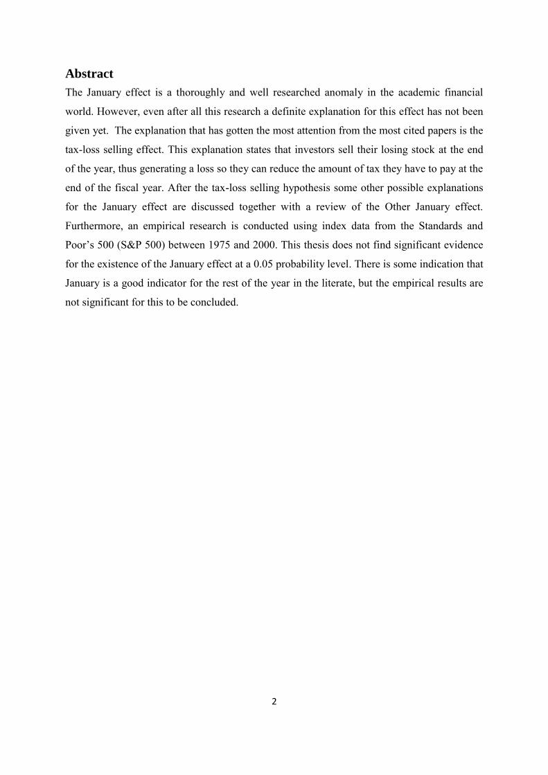
To summarize the results I have created the following table which shows the average capital

and total return of January, the other months (February-December) and all the months

(January-December).

Average monthly capital

return 1975-2000 (%)

Average monthly total

return 1975-2000 (%)

January 1,9033 2,6389

Other months 0,8666 1,2297

All months 0,9530 1,3471

Table 2: Summary of the monthly and capital total return

As the last few tables and charts show the return in January has been significantly higher than

in the others months. January has the highest overall return in both the capital as in the total

return. The mean return in January is more than twice as high as the mean return of all the

other months.

Using these data I can a test whether I can find evidence for the January effect. I need to find

a significant positive difference between the mean return in January and the mean return for

the other months of the year. For this test I have used the following formula:

Rit = Oi + βidit + Eit

Where Rit is the monthly return of the stock market index (i) at time (t), Oi is the average

return of all months other than January, βi will be the difference between the return of January

and the mean of the other months, dit is a dummy variable where i=1 for January and i=0 for

all other months and E is the error term. The sum of the intercept and the slope is equal to the

January mean return.

17

The statistical results are given in the following table using the average monthly capital

returns.

O t-stat β t-stat Jan Mean p-value

S&P 500

1975-2000

0,8666 3,333 1,0367 1,668 1,9033 0.096

Table 3: Test statistics for the January effect

With a p-value of 0.096 we can conclude that the January effect is significant when we use a

0.1 probability level. However, this is one of the lowest confidence levels that are used in

statistics; most researchers test at 0.05 probability level, so I too will also use the 0.05 level

and conclude that I am not able to find evidence for the January effect.

4.2 The Other January effect

After the testing of the January effect, I have also tested the Other January effect. I have tested

whether January is a good indicator for the remainder of the year. In the following table the

results of this research are given. I will be able to provide evidence for this theory if the return

in January will be the same as the return of the entire year, with ‘the same’ being positive in

January and positive over the entire year or negative in January and negative over the entire

year. By using the same S&P 500 data from 1975 to 2000 the following table provides the

distribution of the 26 years in the data.

Yearly return positive Yearly return negative

January return positive 17 1

January return negative 4 4

Table 4: Positive/negative January returns compared to yearly returns

This table shows that in 21 of the 26 years during 1975 and 2000 the return in January gives a

good indication whether the total return of the year is going to be positive or negative. This

equals 80, 77 percent. Before I can conclude whether January is a good indicator I first have

18

to perform a test using a formula that was also used in the papers from Cooper, McConnell

and Ovtchinnikov (2006) and Stivers, Sun and Sun (2009). The formula is as follows:

Rt= a+βjt + et

Where Rt is the 11-month excess return from February to December in year t, βjt is 1 if the

excess return in January is positive, otherwise βjt is 0. βjt should be significantly different than

zero. If β is positive and significant then I have found evidence to support the Other January

effect. An important note is that β can also be interpreted as the spread in returns between

positive and negative January’s. This knowledge is also used in the following table.

The following table gives the results of this test.

Positive Januarys Negative Januarys Spread (%) p-value

Returns

(%)

N Returns

(%)

N

S&P 500

1975-2000

1.07 18 0.24 8 0.83 0.216

Table 5: Test statistics of the Other January effect

With a p-value of 0.216 it cannot be concluded that there is significant relation between

January and the other eleven months. Stivers, Sun and Sun (2009) also used another

regression where the excess January return is used instead of the January dummy as the

explanatory variable. Stivers, Sun and sun conclude that the results are broadly consistent

with the case where the January dummy is used.

19

5. Conclusion

This Chapter will conclude my thesis. After a brief summary of the literature this chapter will

furthermore discuss the findings of the performed empirical research. After that the research

questions stated at the beginning of the thesis will be answered as good as possible. At last

some recommendations for future research will be provided.

5.1 Conclusions & limitations

This thesis started with the Efficient Market Hypothesis from Fama (1970). According to this

theory it should be impossible to beat the market and receive a higher return than the market.

The January effect was one of the anomalies that contradicted the EMH. The existence of the

January effect is well documented. Wachtel (1942) was the first to find significant evidence in

favor of the January effect in the Dow Jones Industrial Index. Rozeff and Kinney (1976)

continued the search for seasonal anomalies in their study on the New York stock exchange.

One of their results was that January had an average return of 3.5% while the other months

only had a mean return of 0.5%. After Rozeff and Kinney more people started to investigate

the January effect, including Reinganum (1983) and Ross (1983) which both found results

that confirmed that there was a January effect.

A fast majority of the research performed states that the tax-loss selling explanation makes the

most economical and financial sense. Among many others, Reinganum (1983) and Ritter

(1988) provide evidence for this hypothesis. However, there are also quite some researchers

that disregard the idea of tax-loss selling being the explanation for the January effect, stating

among other reasons that the effect already existed before capital returns were taxed.

The tax-loss selling hypothesis might be or might not be the best answer to the January effect,

but even now it is still highly debated among the academics. There may also be other reasons

for the January effect. Over the years, there are quite a large amount of other possible

explanations that researchers have addressed as a possible reason for the effect including

window dressing, the release of new information at the end of the (fiscal) year, the firm size

and the possibility of a structure problem. All these other explanations have received enough

attention in the academic world and they just might have something to do with the January

effect. Several reasons how the January effect happens have been discussed in this thesis, but

none can fully explain the phenomenon, even the most popular tax-loss selling hypothesis.

More studies are to be carried out for a better understanding of the January effect.

20

During 1975 and 2000 January was the month with the highest return with and without the

dividend included in the return. While these results may have looked promising, the

performed research on the S&P 500 data does not show significant evidence in favor of the

January effect. In the literature there is quite enough evidence for the existence of the January

effect, but I am not able to significantly prove it in my research with a 0.05 probability level.

This means that the answer to my research question has to be inconclusive.

The Other January effect, which is elaborated in a paper by Cooper, McConnell and

Ovtchinnikov (2006), is a hypothesis that the returns in January are a good indicator for the

stock market return of the rest of the year. There seems to be some evidence in the literature

for this phenomenon, but in my own research I cannot find significant evidence to support this

idea. In 80, 77 percent of the years during 1975-2000 the positive or negative return in

January was the same as in the entire year, which was not enough especially compared to the

other months of the year. A few of the remaining eleven months also performed around this

percentage, which might be one of the reasons why I could not provide enough support for the

Other January effect. My empirical research does not provide significant results to support the

Other January effect. More research has to be performed on this particular phenomenon

before a definite answer can be given.

If the January effect exists it comes to mind that smart investors should be able to take

advantage of this investment opportunity. If you would buy stock at the end of December you

would be able to make a decent profit. If enough investors would use this strategy then the

entire January effect should quickly disappear. There is enough evidence that a January effect

does exist, so there must be a reason why this otherwise profitable strategy does not work.

One of the problems cited by literate is a study by Lakonishok and Smidt (1984) who state

that the opportunity for large profits are hard in a market with small firms, small trading

volumes and large bid-ask spreads. Because of this the ability to generate a large amount of

profit is not as easy as it might sound, especially for individual investors who have to pay

transaction costs. Still, there are some large traders that do not have to face transaction costs.

This is just one of the issues at hand why more research has to be performed on the January

effect.

21

5.2 Recommendations for future research

In this thesis I have mainly focused on the American stock market using data from the S&P

500. Future research can be conducted about other foreign stock indexes like the Chinese or

the Brazilian stock market. It would be interesting to see if seasonal effects like the January

effect are also apparent on other stock market. This would greatly enhance the power of the

conclusions drawn. Another possibility is to expand the data to include the financial crisis. It

would be interesting to see if the January effect also exists in a crisis situation.

Herbst and Slinkman (1984), Huang (1985), Hensel and Ziemba (1995), and Santa-Clara

and Valkanov (2003) report that common stocks earn higher returns when a Democrat is

president than when a Republican is president. With the upcoming presidential elections this

might be an interesting case. It might even be useful in Obama’s campaign. Beside the

presidential anomaly there are many more seasonal phenomenons that are worth looking into.

There is for example the day of the week effect, the turn of the year effect and the holiday

effect.

22

References:

Banz Rolf, The relationships between return and market value of common stocks,

journal of Financial Economics Vol 9,1981, p.3-18.

Basu, S., (1983), “The Relationship between Earnings Yield, Market Value, and

Return for NYSE Common Stocks,” Journal of Financial Economics, 12,

129-156.

De Bondt,W. F. M., and R. Thaler, 1985, Does the stock market overreact?, Journal of

Finance 40, 793-808.

De Bondt, W. F. M., and R. H. Thaler, 1987, Further evidence on investor

overreaction and stock market seasonality, Journal of Finance 42, 557-581.

Fama,Eugene F, Random walks in stock market prices, Financial Analysis

Journal,January-February, 1965, p.75-78.

Fama,Egnene F, Efficient capital markets: A review of Theory and empirical work,

Journal of Finance, May,vol 25 Issue 2, 1970, p.383-417.

Fama,Egene F, Efficient capital markets Ⅱ, Journal of Financ,Vol 46, no. 5, 1991, p.

1575-1617.

Eugene F. Fama and Kenneth R: French, The Cross Section of Expected Stock

Returns, Journal of Finance 47, 1992, p427-65

Gultekin, M. N. And Gultekin, N. B., Stock market seasonality: International

evidence, Journal of Financial Economics, 12, 1983, p.469-81.

Jay R. Ritter, The Buying and Selling Behavior of Individual Investor at the Turn of

the Year, Journal of Finance, 43, July 1988, p.701-17.

23

Keim, D.B., Size-related Anomalies and Stock Return Seasonality: Further Empirical

Evidence,” Journal of Financial Economics, 12 (1983), p.13-32

Kendall, M.,The analysis of economic time series, Journal of the Royal Statistical

Society, Series A,vol.96, 1953, p.11-25.

Lakonishok, J. and Smidt, S., Are seasonal anomalies real? A ninety-year perspective,

Review of Financial Studies, 1, 1988, p403–25

Lakonishok, Josef, Andrei Schleifer, Richard Thaler, and Robert Vishny. 1991.

“Window Dressing by Pension Fund Managers,” American Economic Review, vol. 81,

no. 2 (May 1991): 227-231.

Reinganum, M., The anomalous stock market behavior of small firms in January:

empirical tests for tax-loss selling effects, Journal of Financial Economics, 12, 1983,

p.89-104.

Reinganum, M. R., and A. C., Shapiro., Taxes and stock return seasonality: Evidence

from the London Stock Exchange. Journal of Business, 60, 1987, p.281–95.

Reinganum, Marc R. 1983. “The Anomalous Stock Market Behavior of Small Firms

in January: Empirical Tests for Tax-Loss Selling Effects,” Journal of Financial

Economics, vol. 12, no. 1 (June): 89-104.

Ritter, J. R., 1988, The buying and selling behavior of individual investors at the turn

of the year, Journal of Finance 43, 701-717.

Rogalski, R. J. and Tinic, S., The January size effect: anomaly or risk

mismeasurement? Financial Analyst Journal, 1986, p.63-70.

Roll, R. , The-turn-of-the-year effect and the return premia of small firms, Journal of

Portfolio management, 9, 1983, p.18-28.

24

Rozeff, M. and Kinney, W. , Capital market seasonality: the case of stock returns,

Journal of Financial Economics, 3, 1976, p.379-402.

Sanjoy Basu, The Investment Performance of Common Stocks in Relation to Their

Price-Earnings Ratios: A Test of the Efficient Market Hypothesis, Journal of Finance

32, June 1977, p663-82.

Schwert, G. W., 2003, Anomalies and Market Efficiency, Chapter 15, Handbook of

the Economics of Finance, eds. G. Constantinides, M. Harris, R. Stulz, and North-

Holland, 937-972.

Sullivan, Ryan, Allan Timmerman, and Halbert White. 2001. “Dangers of Data

Mining: The Case of Calendar Effects in Stock Returns,” Journal of Econometrics,

vol. 105, no. 1 (November): 249-286.

Szakmary, Andrew C. and Dean B. Kiefer. 2004. “The Disappearing January/Turn Of

The Year Effect: Evidence From Stock Index Futures And Cash Markets,” Journal of

Futures Markets, vol. 24, no. 8 (August): 755-784.

Thaler, R., De Bondt, W.F.M., (1985) “Does the stock market overreact?” The journal

of Finance (40)3 793-805.

Thaler, Richard H. 1987, “Amomalies: The January Effect, “ The Journal of Economic

perspectives, Vol. 1, No. 1, 197-201.