Embed Size (px)
Citation preview
Portfolio Optimization with R/Rmetrics
Rmetrics Association & Finance Online
Diethelm WürtzYohan ChalabiWilliam ChenAndrew Ellis
�Sam
ple

Sample
Diethelm WürtzYohan ChalabiWilliam ChenAndrew Ellis
Portfolio Optimizationwith R/Rmetrics
May 11, 2009
Rmetrics Association & Finance OnlineZurich
Sample

Sample

Sample
Series Editors:PD Dr. Diethelm WürtzInstitute of Theoretical Physics andCurriculum for Computational ScienceSwiss Federal Institute of TechnologyHönggerberg, HIT K 32.28093 Zurich
Dr. Martin HanfFinance Online GmbHWeinbergstrasse 418006 Zurich
Contact Address:Rmetrics AssociationWeinbergstrasse 418006 [email protected]
Publisher:Finance Online GmbHSwiss Information TechnologiesWeinbergstrasse 418006 Zurich
Authors:Yohan Chalabi, ETH ZurichWilliam Chen, University of AucklandAndrew Ellis, Finance Online GmbH ZurichDiethelm Würtz, ETH Zurich
ISBN:eISBN:DOI:
© 2009, Finance Online GmbH, ZurichAll rights reserved. This work may not be translated or copied in whole or in part withoutthe written permission of the publisher (Finance Online GmbH) except for brief excerptsin connection with reviews or scholarly analysis. Use in connection with any form ofinformation storage and retrieval, electronic adaptation, computer software, or by similaror dissimilar methodology now known or hereafter developed is forbidden.
Limit of Liability/Disclaimer of Warranty: While the publisher and authors have usedtheir best efforts in preparing this book, they make no representations or warrantieswith respect to the accuracy or completeness of the contents of this book and specificallydisclaim any implied warranties of merchantability or fitness for a particular purpose. Nowarranty may be created or extended by sales representatives or written sales materials.The advice and strategies contained herein may not be suitable for your situation. Youshould consult with a professional where appropriate. Neither the publisher nor authorsshall be liable for any loss of profit or any other commercial damages, including but notlimited to special, incidental, consequential, or other damages.
Trademark notice: Product or corporate names may be trademarks or registered trade-marks, and are used only for identification and explanation, without intent to infringe.
Sample

vii
Revision History
May 2009: 1st editionVersion control information : Revision 1087
Sample
Contents
Preface xi
Contents xvii
List of Figures xxv
List of R Code xxix
List of Abbreviations xxxiii
Introduction 1
Part I Managing Data Sets of Assets 3
Introduction 5
1 Generic Functions to Manipulate Assets 7
1.1 timeDate and timeSeries Objects . . . . . . . . . . . . . . . . . . . . 81.2 Loading timeSeries Data Sets . . . . . . . . . . . . . . . . . . . . . . 91.3 Sorting and Reverting Assets . . . . . . . . . . . . . . . . . . . . . . 111.4 Alignment of Assets . . . . . . . . . . . . . . . . . . . . . . . . . . 141.5 Binding and Merging Assets . . . . . . . . . . . . . . . . . . . . . . 151.6 Subsetting Assets . . . . . . . . . . . . . . . . . . . . . . . . . . . . 20
xvii
Sample
xviii Contents
1.7 Aggregating Assets . . . . . . . . . . . . . . . . . . . . . . . . . . . 231.8 Rolling Assets . . . . . . . . . . . . . . . . . . . . . . . . . . . . . 25
2 Financial Functions to Manipulate Assets 31
2.1 Price and Index Series . . . . . . . . . . . . . . . . . . . . . . . . . 312.2 Return and Cumulated Return Series . . . . . . . . . . . . . . . . . 322.3 Drawdowns Series . . . . . . . . . . . . . . . . . . . . . . . . . . . 342.4 Durations Series . . . . . . . . . . . . . . . . . . . . . . . . . . . . 352.5 How to Add Your Own Functions . . . . . . . . . . . . . . . . . . . 36
3 Basic Statistics of Financial Assets 41
3.1 Summary Statistics . . . . . . . . . . . . . . . . . . . . . . . . . . . 413.2 Sample Mean and Covariance Estimates . . . . . . . . . . . . . . . . 443.3 Estimates for Higher Moments . . . . . . . . . . . . . . . . . . . . . 463.4 Quantiles and Related Risk Measures . . . . . . . . . . . . . . . . . 473.5 Computing Column Statistics . . . . . . . . . . . . . . . . . . . . . 493.6 Computing Cumulated Column Statistics . . . . . . . . . . . . . . . 50
4 Robust Mean and Covariance Estimates of Assets 51
4.1 Robust Covariance Estimators . . . . . . . . . . . . . . . . . . . . . 524.2 Comparisons of Robust Covariances . . . . . . . . . . . . . . . . . . 544.3 Minimum Volume Ellipsoid Estimator . . . . . . . . . . . . . . . . . 544.4 Minimum Covariance Determinant Estimator . . . . . . . . . . . . . 554.5 Orthogonalized Gnanadesikan-Kettenring Estimator . . . . . . . . . . 594.6 Nearest-Neighbour Variance Estimator . . . . . . . . . . . . . . . . . 594.7 Shrinkage Estimator . . . . . . . . . . . . . . . . . . . . . . . . . . 614.8 Bagging Estimator . . . . . . . . . . . . . . . . . . . . . . . . . . . 624.9 How to Add a New Estimator to the Suite . . . . . . . . . . . . . . . 634.10 How to Detect Outliers in a Set of Assets . . . . . . . . . . . . . . . 64
Part II Exploratory Data Analysis of Assets 67
Introduction 69
Personal Copy of [email protected] – Please do not distribute
Sample
Contents xix
5 Plotting Financial Time Series And Their Properties 71
5.1 Financial Time Series Plots . . . . . . . . . . . . . . . . . . . . . . . 715.2 Box Plots . . . . . . . . . . . . . . . . . . . . . . . . . . . . . . . . 835.3 Histogram and Density Plots . . . . . . . . . . . . . . . . . . . . . . 875.4 Quantile-Quantile Plots . . . . . . . . . . . . . . . . . . . . . . . . 90
6 Customization of Plots 95
6.1 Plot Labels . . . . . . . . . . . . . . . . . . . . . . . . . . . . . . . 956.2 More About Plot Function Arguments . . . . . . . . . . . . . . . . . 986.3 Selecting Colours . . . . . . . . . . . . . . . . . . . . . . . . . . . . 1026.4 Selecting Character Fonts . . . . . . . . . . . . . . . . . . . . . . . . 1096.5 Selecting Plot Symbols . . . . . . . . . . . . . . . . . . . . . . . . . 112
7 Modelling Assets Returns 117
7.1 Testing Assets Returns for Normality . . . . . . . . . . . . . . . . . . 1177.2 Fitting Assets Returns . . . . . . . . . . . . . . . . . . . . . . . . . 1207.3 Simulating Asset Returns from a given Distribution . . . . . . . . . . 123
8 Selecting Similar or Dissimilar Assets 125
8.1 Functions for Grouping Similar Assets . . . . . . . . . . . . . . . . . 1258.2 Grouping Asset Returns by Hierarchical Clustering . . . . . . . . . . 1268.3 Grouping Asset Returns by k-means Clustering . . . . . . . . . . . . 1318.4 Grouping Asset Returns through Eigenvalue Analysis . . . . . . . . . 1338.5 Grouping Asset Returns by Contributed Cluster Algorithms . . . . . . 1338.6 Ordering Data Sets of Assets . . . . . . . . . . . . . . . . . . . . . . 137
9 Comparing Multivariate Return and Risk Statistics 139
9.1 Stars and Segments Plots . . . . . . . . . . . . . . . . . . . . . . . . 1399.2 Segments Plots of Basic Return Statistics . . . . . . . . . . . . . . . . 1419.3 Segments Plots of Distribution Moments . . . . . . . . . . . . . . . . 1419.4 Segments Plots of Box Plot Statistics . . . . . . . . . . . . . . . . . . 1449.5 How to Position Stars and Segments in Stars Plots . . . . . . . . . . . 144
10 Pairwise Dependencies of Assets 147
10.1 Simple Pairwise Scatter Plots of Assets . . . . . . . . . . . . . . . . . 147
Sample
xx Contents
10.2 Pairwise Correlations Between Assets . . . . . . . . . . . . . . . . . 15210.3 Tests of Pairwise Correlations . . . . . . . . . . . . . . . . . . . . . 15610.4 Image Plot of Correlations . . . . . . . . . . . . . . . . . . . . . . . 15710.5 Bivariate Histogram Plots . . . . . . . . . . . . . . . . . . . . . . . 159
Part III Portfolio Framework 165
Introduction 167
11 S4 Portfolio Specification Class 169
11.1 Class Representation . . . . . . . . . . . . . . . . . . . . . . . . . . 16911.2 The Model Slot . . . . . . . . . . . . . . . . . . . . . . . . . . . . . 17411.3 The Portfolio Slot . . . . . . . . . . . . . . . . . . . . . . . . . . . . 17911.4 The Optim Slot . . . . . . . . . . . . . . . . . . . . . . . . . . . . . 18411.5 The Message Slot . . . . . . . . . . . . . . . . . . . . . . . . . . . . 18711.6 Consistency Checks on Specifications . . . . . . . . . . . . . . . . . 188
12 S4 Portfolio Data Class 189
12.1 Class Representation . . . . . . . . . . . . . . . . . . . . . . . . . . 18912.2 The Data Slot . . . . . . . . . . . . . . . . . . . . . . . . . . . . . . 19312.3 The Statistics Slot . . . . . . . . . . . . . . . . . . . . . . . . . . . . 193
13 S4 Portfolio Constraints Class 197
13.1 Class Representation . . . . . . . . . . . . . . . . . . . . . . . . . . 19713.2 Long-Only Constraints String . . . . . . . . . . . . . . . . . . . . . 20013.3 Unlimited Short Selling Constraints String . . . . . . . . . . . . . . . 20213.4 Box Constraints Strings . . . . . . . . . . . . . . . . . . . . . . . . . 20213.5 Group Constraints Strings . . . . . . . . . . . . . . . . . . . . . . . 20413.6 Covariance Risk Budget Constraints Strings . . . . . . . . . . . . . . 20513.7 Non-Linear Weight Constraints Strings . . . . . . . . . . . . . . . . . 20713.8 Case study: How To Construct Complex Portfolio Constraints . . . . . 208
14 Portfolio Functions 213
14.1 S4 Class Representation . . . . . . . . . . . . . . . . . . . . . . . . 213
Personal Copy of [email protected] – Please do not distribute
Sample
Contents xxi
Part IV Mean-Variance Portfolios 219
Introduction 221
15 Markowitz Portfolio Theory 223
15.1 The Minimum Risk Mean-Variance Portfolio . . . . . . . . . . . . . . 22315.2 The Feasible Set and the Efficient Frontier . . . . . . . . . . . . . . . 22515.3 The Minimum Variance Portfolio . . . . . . . . . . . . . . . . . . . . 22515.4 The Capital Market Line and Tangency Portfolio . . . . . . . . . . . . 22515.5 Box and Group Constrained Mean-Variance Portfolios . . . . . . . . . 22715.6 Maximum Return Mean-Variance Portfolios . . . . . . . . . . . . . . 22815.7 Covariance Risk Budgets Constraints . . . . . . . . . . . . . . . . . . 228
16 Mean-Variance Portfolio Settings 231
16.1 Step 1: Portfolio Data . . . . . . . . . . . . . . . . . . . . . . . . . . 23116.2 Step 2: Portfolio Specification . . . . . . . . . . . . . . . . . . . . . . 23216.3 Step 3: Portfolio Constraints . . . . . . . . . . . . . . . . . . . . . . 233
17 Minimum Risk Mean-Variance Portfolios 235
17.1 How to Compute a Feasible Portfolio . . . . . . . . . . . . . . . . . . 23517.2 How to Compute a Minimum Risk Efficient Portfolio . . . . . . . . . 23817.3 How to Compute the Global Minimum Variance Portfolio . . . . . . . 23917.4 How to Compute the Tangency Portfolio . . . . . . . . . . . . . . . . 24317.5 How to Customize a Pie Plot . . . . . . . . . . . . . . . . . . . . . . 244
18 Mean-Variance Portfolio Frontiers 247
18.1 Frontier Computation and Graphical Displays . . . . . . . . . . . . . 24718.2 The ‘long-only’ Portfolio Frontier . . . . . . . . . . . . . . . . . . . . 25218.3 The Unlimited ‘short’ Portfolio Frontier . . . . . . . . . . . . . . . . 25618.4 The Box-Constrained Portfolio Frontier . . . . . . . . . . . . . . . . . 25718.5 The Group-Constrained Portfolio Frontier . . . . . . . . . . . . . . . 26118.6 The Box/Group-Constrained Portfolio Frontier . . . . . . . . . . . . . 26518.7 Creating Different ‘Reward/Risk Views’ on the Efficient Frontier . . . . 270
19 Case Study: Dow Jones Index 273
Sample
xxii Contents
20 Robust Portfolios and Covariance Estimation 277
20.1 Robust Mean and Covariance Estimators . . . . . . . . . . . . . . . . 27820.2 The MCD Robustified Mean-Variance Portfolio . . . . . . . . . . . . . 27920.3 The MVE Robustified Mean-Variance Portfolio . . . . . . . . . . . . . 28120.4 The OGK Robustified Mean-Variance Portfolio . . . . . . . . . . . . . 28720.5 The Shrinked Mean-Variance Portfolio . . . . . . . . . . . . . . . . . 29220.6 How to Write Your Own Covariance Estimator . . . . . . . . . . . . . 293
Part V Mean-CVaR Portfolios 301
Introduction 301
21 Mean-CVaR Portfolio Theory 303
21.1 Solution of the Mean-CVaR Portfolio . . . . . . . . . . . . . . . . . . 30421.2 Discretization . . . . . . . . . . . . . . . . . . . . . . . . . . . . . 30521.3 Linearization . . . . . . . . . . . . . . . . . . . . . . . . . . . . . . 307
22 Mean-CVaR Portfolio Settings 309
22.1 Step 1: Portfolio Data . . . . . . . . . . . . . . . . . . . . . . . . . . 30922.2 Step 2: Portfolio Specification . . . . . . . . . . . . . . . . . . . . . . 30922.3 Step 3: Portfolio Constraints . . . . . . . . . . . . . . . . . . . . . . 311
23 Mean-CVaR Portfolios 313
23.1 How to Compute a Feasible Mean-CVaR Portfolio . . . . . . . . . . . 31323.2 How to Compute the Mean-CVaR Portfolio with the Lowest Risk for a
Given Return . . . . . . . . . . . . . . . . . . . . . . . . . . . . . . 31623.3 How to Compute the Global Minimum Mean-CVaR Portfolio . . . . . 317
24 Mean-CVaR Portfolio Frontiers 323
24.1 The Long-only Portfolio Frontier . . . . . . . . . . . . . . . . . . . . 32424.2 The Unlimited ‘Short’ Portfolio Frontier . . . . . . . . . . . . . . . . 32624.3 The Box-Constrained Portfolio Frontier . . . . . . . . . . . . . . . . . 33224.4 The Group-Constrained Portfolio Frontier . . . . . . . . . . . . . . . 33324.5 The Box/Group-Constrained Portfolio Frontier . . . . . . . . . . . . . 339
Personal Copy of [email protected] – Please do not distribute
Sample
Contents xxiii
24.6 Other Constraints . . . . . . . . . . . . . . . . . . . . . . . . . . . 34024.7 More About the Frontier Plot Tools . . . . . . . . . . . . . . . . . . 340
Part VI Portfolio Backtesting 347
Introduction 349
25 S4 Portfolio Backtest Class 351
25.1 Class Representation . . . . . . . . . . . . . . . . . . . . . . . . . . 35125.2 The Windows Slot . . . . . . . . . . . . . . . . . . . . . . . . . . . 35325.3 The Strategy Slot . . . . . . . . . . . . . . . . . . . . . . . . . . . . 35825.4 The Smoother Slot . . . . . . . . . . . . . . . . . . . . . . . . . . . 36025.5 Rolling Analysis . . . . . . . . . . . . . . . . . . . . . . . . . . . . 365
26 Case Study: SPI Sector Rotation 375
26.1 SPI Portfolio Backtesting . . . . . . . . . . . . . . . . . . . . . . . . 37526.2 SPI Portfolio Weights Smoothing . . . . . . . . . . . . . . . . . . . . 37726.3 SPI Portfolio Backtest Plots . . . . . . . . . . . . . . . . . . . . . . . 37726.4 SPI Performance Review . . . . . . . . . . . . . . . . . . . . . . . . 378
27 Case Study: GCC Index Rotation 381
27.1 GCC Portfolio Weights Smoothing . . . . . . . . . . . . . . . . . . . 38227.2 GCC Performance Review . . . . . . . . . . . . . . . . . . . . . . . 38427.3 Alternative Strategy . . . . . . . . . . . . . . . . . . . . . . . . . . 384
Part VII Appendix 387
A Packages Required for this ebook 389
B Description of Data Sets 399
B.1 Data Set: SWX . . . . . . . . . . . . . . . . . . . . . . . . . . . . . 399B.2 Data Set: LPP2005 . . . . . . . . . . . . . . . . . . . . . . . . . . . 400B.3 Data Set: SPISECTOR . . . . . . . . . . . . . . . . . . . . . . . . . 400B.4 Data Set: SMALLCAP . . . . . . . . . . . . . . . . . . . . . . . . . 401
Sample

xxiv Contents
B.5 Data Set: GCCINDEX . . . . . . . . . . . . . . . . . . . . . . . . . 402
Bibliography 403
Index 408
About the Authors 411
Personal Copy of [email protected] – Please do not distribute
Sample
Chapter 20
Robust Portfolios and Covariance Estimation
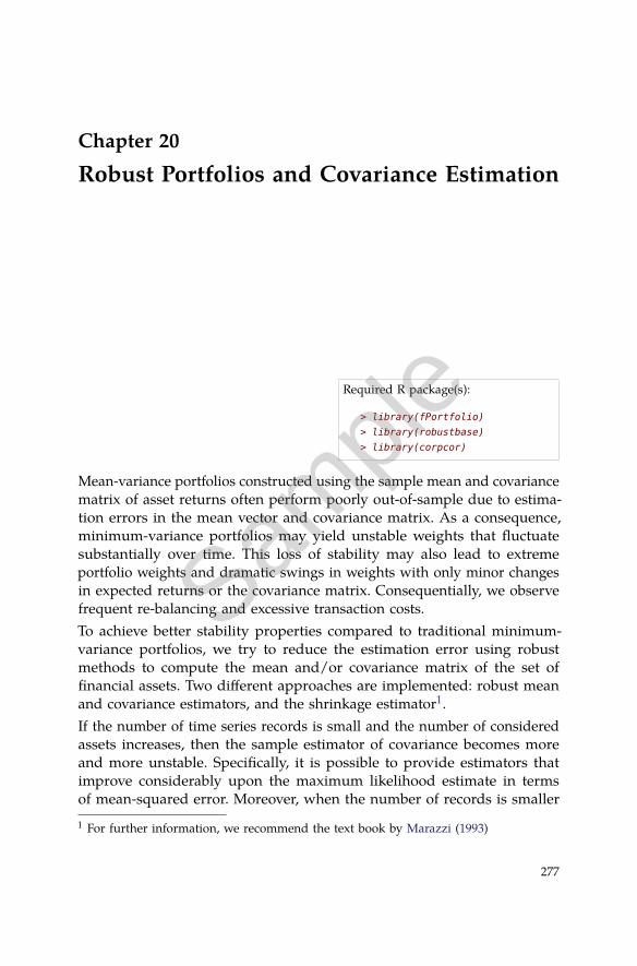
Required R package(s):
> library(fPortfolio)
> library(robustbase)
> library(corpcor)
Mean-variance portfolios constructed using the sample mean and covariancematrix of asset returns often perform poorly out-of-sample due to estima-tion errors in the mean vector and covariance matrix. As a consequence,minimum-variance portfolios may yield unstable weights that fluctuatesubstantially over time. This loss of stability may also lead to extremeportfolio weights and dramatic swings in weights with only minor changesin expected returns or the covariance matrix. Consequentially, we observefrequent re-balancing and excessive transaction costs.To achieve better stability properties compared to traditional minimum-variance portfolios, we try to reduce the estimation error using robustmethods to compute the mean and/or covariance matrix of the set offinancial assets. Two different approaches are implemented: robust meanand covariance estimators, and the shrinkage estimator1.If the number of time series records is small and the number of consideredassets increases, then the sample estimator of covariance becomes moreand more unstable. Specifically, it is possible to provide estimators thatimprove considerably upon the maximum likelihood estimate in termsof mean-squared error. Moreover, when the number of records is smaller1 For further information, we recommend the text book by Marazzi (1993)
277
Sample
278 20 Robust Portfolios and Covariance Estimation
than the number of assets, the empirical estimate of the covariance matrixbecomes singular.
20.1 Robust Mean and Covariance Estimators
In the mean-variance portfolio approach, the sample mean and samplecovariance estimators are used by default to estimate the mean vector andcovariance matrix.This information, i.e. the name of the covariance estimator function, is keptin the specification structure and can be shown by calling the functiongetEstimator(). The default setting is
> getEstimator(portfolioSpec())
[1] "covEstimator"
There are many different implementations of robust and related estimatorsfor the mean and covariance in R’s base packages and in contributedpackages. The estimators listed below can be accessed by the portfoliooptimization program.
Functions:
covEstimator Covariance sample estimator
kendallEstimator Kendall's rank estimator
spearmanEstimator Spearman's rank estimator
mcdEstimator MCD, minimum covariance determinant estimator
mveEstimator MVE, minimum volume ellipsoid estimator
covMcdEstimator Minimum covariance determinant estimator
covOGKEstimator Orthogonalized Gnanadesikan-Kettenring estimator
shrinkEstimator Shrinkage covariance estimator
baggedEstimator Bagged covariance estimator
Listing 20.1 Rmetrics functions to estimate robust covariances for portfolio optimization
Personal Copy of [email protected] – Please do not distribute
Sample
20.2 The MCD Robustified Mean-Variance Portfolio 279
20.2 The MCD Robustified Mean-Variance Portfolio
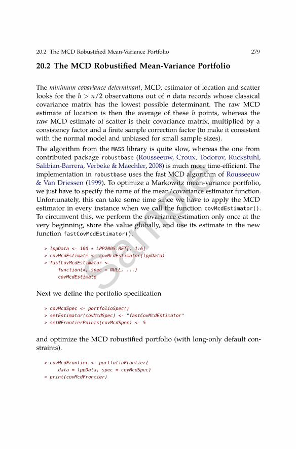
The minimum covariance determinant, MCD, estimator of location and scatterlooks for the h > n/2 observations out of n data records whose classicalcovariance matrix has the lowest possible determinant. The raw MCDestimate of location is then the average of these h points, whereas theraw MCD estimate of scatter is their covariance matrix, multiplied by aconsistency factor and a finite sample correction factor (to make it consistentwith the normal model and unbiased for small sample sizes).The algorithm from the MASS library is quite slow, whereas the one fromcontributed package robustbase (Rousseeuw, Croux, Todorov, Ruckstuhl,Salibian-Barrera, Verbeke & Maechler, 2008) is much more time-efficient. Theimplementation in robustbase uses the fast MCD algorithm of Rousseeuw& Van Driessen (1999). To optimize a Markowitz mean-variance portfolio,we just have to specify the name of the mean/covariance estimator function.Unfortunately, this can take some time since we have to apply the MCDestimator in every instance when we call the function covMcdEstimator().To circumvent this, we perform the covariance estimation only once at thevery beginning, store the value globally, and use its estimate in the newfunction fastCovMcdEstimator().
> lppData <- 100 * LPP2005.RET[, 1:6]
> covMcdEstimate <- covMcdEstimator(lppData)
> fastCovMcdEstimator <-
function(x, spec = NULL, ...)
covMcdEstimate
Next we define the portfolio specification
> covMcdSpec <- portfolioSpec()
> setEstimator(covMcdSpec) <- "fastCovMcdEstimator"
> setNFrontierPoints(covMcdSpec) <- 5
and optimize the MCD robustified portfolio (with long-only default con-straints).
> covMcdFrontier <- portfolioFrontier(
data = lppData, spec = covMcdSpec)
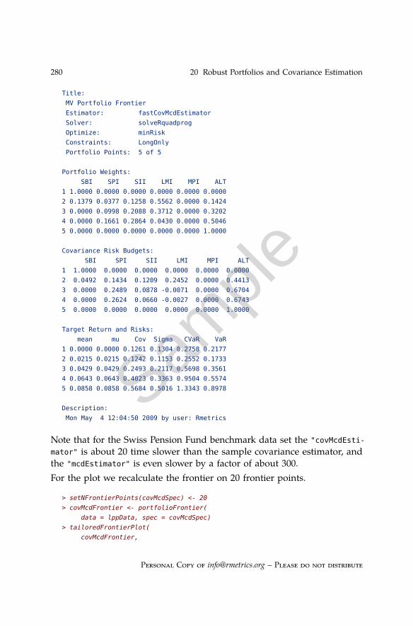
> print(covMcdFrontier)
Sample
280 20 Robust Portfolios and Covariance Estimation
Title:
MV Portfolio Frontier
Estimator: fastCovMcdEstimator
Solver: solveRquadprog
Optimize: minRisk
Constraints: LongOnly
Portfolio Points: 5 of 5
Portfolio Weights:
SBI SPI SII LMI MPI ALT
1 1.0000 0.0000 0.0000 0.0000 0.0000 0.0000
2 0.1379 0.0377 0.1258 0.5562 0.0000 0.1424
3 0.0000 0.0998 0.2088 0.3712 0.0000 0.3202
4 0.0000 0.1661 0.2864 0.0430 0.0000 0.5046
5 0.0000 0.0000 0.0000 0.0000 0.0000 1.0000
Covariance Risk Budgets:
SBI SPI SII LMI MPI ALT
1 1.0000 0.0000 0.0000 0.0000 0.0000 0.0000
2 0.0492 0.1434 0.1209 0.2452 0.0000 0.4413
3 0.0000 0.2489 0.0878 -0.0071 0.0000 0.6704
4 0.0000 0.2624 0.0660 -0.0027 0.0000 0.6743
5 0.0000 0.0000 0.0000 0.0000 0.0000 1.0000
Target Return and Risks:
mean mu Cov Sigma CVaR VaR
1 0.0000 0.0000 0.1261 0.1304 0.2758 0.2177
2 0.0215 0.0215 0.1242 0.1153 0.2552 0.1733
3 0.0429 0.0429 0.2493 0.2117 0.5698 0.3561
4 0.0643 0.0643 0.4023 0.3363 0.9504 0.5574
5 0.0858 0.0858 0.5684 0.5016 1.3343 0.8978
Description:
Mon May 4 12:04:50 2009 by user: Rmetrics
Note that for the Swiss Pension Fund benchmark data set the "covMcdEsti-
mator" is about 20 time slower than the sample covariance estimator, andthe "mcdEstimator" is even slower by a factor of about 300.For the plot we recalculate the frontier on 20 frontier points.
> setNFrontierPoints(covMcdSpec) <- 20
> covMcdFrontier <- portfolioFrontier(
data = lppData, spec = covMcdSpec)
> tailoredFrontierPlot(
covMcdFrontier,
Personal Copy of [email protected] – Please do not distribute
Sample
20.3 The MVE Robustified Mean-Variance Portfolio 281
mText = "MCD Robustified MV Portfolio",
risk = "Sigma")
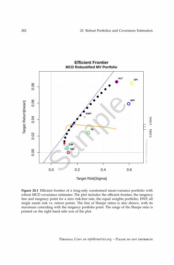
The frontier plot is shown in Figure 20.1.To display the weights, risk attributions and covariance risk budgets for theMCD robustified portfolio in the left-hand column and the same plots forthe sample covariance MV portfolio in the right-hand column of a figure:
> ## MCD robustified portfolio
> par(mfcol = c(3, 2), mar = c(3.5, 4, 4, 3) + 0.1)
> col = qualiPalette(30, "Dark2")
> weightsPlot(covMcdFrontier, mtext = FALSE, col = col)
> text <- "MCD"
> mtext(text, side = 3, line = 3, font = 2, cex = 0.9)
> weightedReturnsPlot(covMcdFrontier, mtext = FALSE, col = col)
> covRiskBudgetsPlot(covMcdFrontier, mtext = FALSE, col = col)
> ## Sample covariance MV portfolio
> longSpec <- portfolioSpec()
> setNFrontierPoints(longSpec) <- 20
> longFrontier <- portfolioFrontier(data = lppData, spec = longSpec)
> col = qualiPalette(30, "Set1")
> weightsPlot(longFrontier, mtext = FALSE, col = col)
> text <- "COV"
> mtext(text, side = 3, line = 3, font = 2, cex = 0.9)
> weightedReturnsPlot(longFrontier, mtext = FALSE, col = col)
> covRiskBudgetsPlot(longFrontier, mtext = FALSE, col = col)
The weights, risk attributions and covariance risk budgets are shown inFigure 20.2.
20.3 The MVE Robustified Mean-Variance Portfolio
Rousseeuw & Leroy (1987) proposed a very robust alternative to clas-sical estimates of mean vectors and covariance matrices, the MinimumVolume Ellipsoid, MVE. Samples from a multivariate normal distributionform ellipsoid-shaped ‘clouds’ of data points. The MVE corresponds tothe smallest point cloud containing at least half of the observations, theuncontaminated portion of the data. These ‘clean’ observations are used forpreliminary estimates of the mean vector and the covariance matrix. Using
Sample
282 20 Robust Portfolios and Covariance Estimation
0.0 0.2 0.4 0.6
0.00
0.02
0.04
0.06
0.08
●
●
●
●
●
●
●
●
●
●
●
●
●
●
●
●
●
●
●
●M
V |
solv
eRqu
adpr
og
Efficient Frontier
Target Risk[Sigma]
Targ
et R
etur
n[m
ean]
MCD Robustified MV Portfolio
●
●
EWP
●
●
●
●
●
●
SBI
SPI
SII
LMI
MPI
ALT
0.02
81
0.0
341
Figure 20.1 Efficient frontier of a long-only constrained mean-variance portfolio withrobust MCD covariance estimates: The plot includes the efficient frontier, the tangencyline and tangency point for a zero risk-free rate, the equal weights portfolio, EWP, allsingle assets risk vs. return points. The line of Sharpe ratios is also shown, with itsmaximum coinciding with the tangency portfolio point. The range of the Sharpe ratio isprinted on the right hand side axis of the plot.
Personal Copy of [email protected] – Please do not distribute
Sample
20.3 The MVE Robustified Mean-Variance Portfolio 2830.
00.
40.
8 SBISPISIILMIMPIALT
0.0
0.4
0.8
0.126 0.15 0.329 0.54
4.07e−05 0.0542 0.0813
Target Risk
Target Return
Wei
ght
Weights MCD
0.00
0.04
0.08 SBI
SPISIILMIMPIALT
0.00
0.04
0.08
0.126 0.15 0.329 0.54
4.07e−05 0.0542 0.0813
Target Risk
Target Return
Wei
ghte
d R
etur
n
Weighted Returns
0.0
0.4
0.8
SBISPISIILMIMPIALT
0.0
0.4
0.8
0.126 0.15 0.329 0.54
4.07e−05 0.0542 0.0813
Target Risk
Target Return
Cov
Ris
k B
udge
ts
Cov Risk Budgets
0.0
0.4
0.8 SBI
SPISIILMIMPIALT
0.0
0.4
0.8
0.126 0.147 0.322 0.529
4.07e−05 0.0542 0.0813
Target Risk
Target ReturnW
eigh
t
Weights COV
0.00
0.04
0.08 SBI
SPISIILMIMPIALT
0.00
0.04
0.08
0.126 0.147 0.322 0.529
4.07e−05 0.0542 0.0813
Target Risk
Target Return
Wei
ghte
d R
etur
n
Weighted Returns
0.0
0.4
0.8
SBISPISIILMIMPIALT
0.0
0.4
0.8
0.126 0.147 0.322 0.529
4.07e−05 0.0542 0.0813
Target Risk
Target Return
Cov
Ris
k B
udge
ts
Cov Risk Budgets
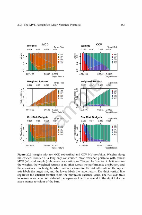
Figure 20.2 Weights plot for MCD robustified and COV MV portfolios. Weights alongthe efficient frontier of a long-only constrained mean-variance portfolio with robustMCD (left) and sample (right) covariance estimates: The graphs from top to bottom showthe weights, the weighted returns or in other words the performance attribution, andthe covariance risk budgets, which are a measure for the risk attribution. The upperaxis labels the target risk, and the lower labels the target return. The thick vertical lineseparates the efficient frontier from the minimum variance locus. The risk axis thusincreases in value to both sides of the separator line. The legend to the right links theassets names to colour of the bars.
Sample
284 20 Robust Portfolios and Covariance Estimation
these estimates, the program computes a robust Mahalanobis distance forevery observation vector in the sample. Observations for which the robustMahalanobis distances exceed the 97.5% significance level for the chi-squaredistribution are flagged as probable outliers.Rmetrics provides a function, mveEstimator(), to compute the MVE estima-tor; it is based on the cov.rob() estimator from the MASS package. We definea function called fastMveEstimator()
> mveEstimate <- mveEstimator(lppData)
> fastMveEstimator <- function(x, spec = NULL, ...) mveEstimate
and set the portfolio specifications
> mveSpec <- portfolioSpec()
> setEstimator(mveSpec) <- "fastMveEstimator"
> setNFrontierPoints(mveSpec) <- 5
Then we compute the MVE robustified efficient frontier
> mveFrontier <- portfolioFrontier(
data = lppData,
spec = mveSpec,
constraints = "LongOnly")
> print(mveFrontier)
Title:
MV Portfolio Frontier
Estimator: fastMveEstimator
Solver: solveRquadprog
Optimize: minRisk
Constraints: LongOnly
Portfolio Points: 5 of 5
Portfolio Weights:
SBI SPI SII LMI MPI ALT
1 1.0000 0.0000 0.0000 0.0000 0.0000 0.0000
2 0.1188 0.0271 0.1520 0.5566 0.0000 0.1455
3 0.0000 0.0709 0.2643 0.3290 0.0000 0.3358
4 0.0000 0.1196 0.3433 0.0000 0.0000 0.5371
5 0.0000 0.0000 0.0000 0.0000 0.0000 1.0000
Covariance Risk Budgets:
SBI SPI SII LMI MPI ALT
1 1.0000 0.0000 0.0000 0.0000 0.0000 0.0000
Personal Copy of [email protected] – Please do not distribute
Sample
20.3 The MVE Robustified Mean-Variance Portfolio 285
2 0.0420 0.0974 0.1682 0.2477 0.0000 0.4447
3 0.0000 0.1693 0.1313 -0.0088 0.0000 0.7082
4 0.0000 0.1819 0.0894 0.0000 0.0000 0.7287
5 0.0000 0.0000 0.0000 0.0000 0.0000 1.0000
Target Return and Risks:
mean mu Cov Sigma CVaR VaR
1 0.0000 0.0000 0.1261 0.1229 0.2758 0.2177
2 0.0215 0.0215 0.1230 0.1094 0.2468 0.1728
3 0.0429 0.0429 0.2465 0.2024 0.5479 0.3459
4 0.0643 0.0643 0.3977 0.3221 0.9183 0.5535
5 0.0858 0.0858 0.5684 0.4781 1.3343 0.8978
Description:
Mon May 4 12:04:54 2009 by user: Rmetrics
For the frontier plot, we recompute the robustified frontier on 20 points.
> setNFrontierPoints(mveSpec) <- 20
> mveFrontier <- portfolioFrontier(
data = lppData, spec = mveSpec)
> tailoredFrontierPlot(
mveFrontier,
mText = "MVE Robustified MV Portfolio",
risk = "Sigma")
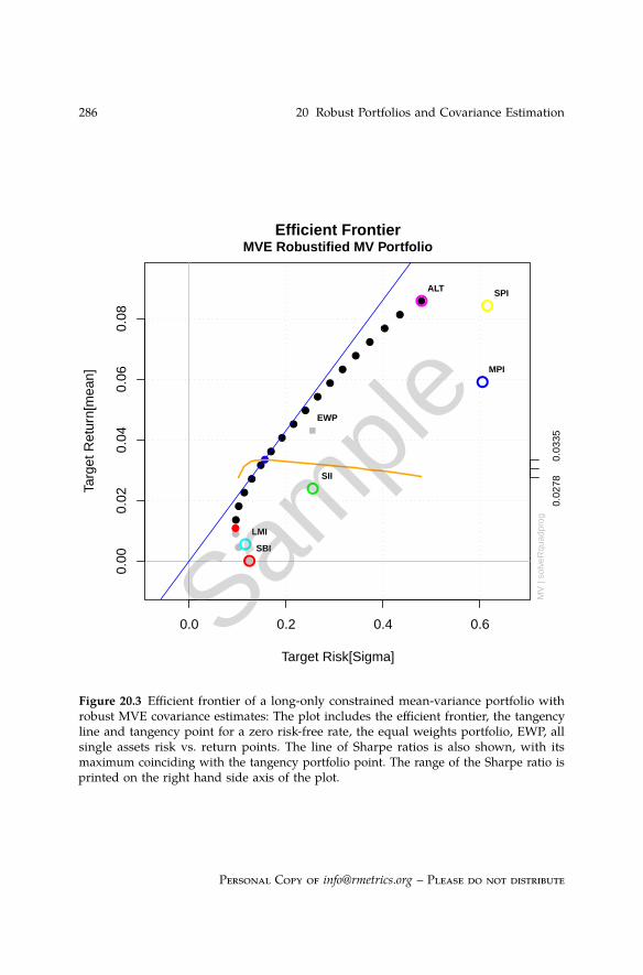
The frontier plot is shown in Figure 20.3.To complete this section, we will show the weights and the performanceand risk attribution plots (left-hand column of Figure 20.4).
> col = divPalette(6, "RdBu")
> weightsPlot(mveFrontier, col = col,
mtext = FALSE)
> boxL()
> text <- "MVE Robustified MV Portfolio"
> mtext(text, side = 3, line = 3, font = 2, cex = 0.9)
> weightedReturnsPlot(mveFrontier, col = col,
mtext = FALSE)
> boxL()
> covRiskBudgetsPlot(mveFrontier, col = col,
mtext = FALSE)
> boxL()
Sample
286 20 Robust Portfolios and Covariance Estimation
0.0 0.2 0.4 0.6
0.00
0.02
0.04
0.06
0.08
●
●
●
●
●
●
●
●
●
●
●
●
●
●
●
●
●
●
●
●M
V |
solv
eRqu
adpr
og
Efficient Frontier
Target Risk[Sigma]
Targ
et R
etur
n[m
ean]
MVE Robustified MV Portfolio
●
●
EWP
●
●
●
●
●
●
SBI
SPI
SII
LMI
MPI
ALT
0.02
78
0.0
335
Figure 20.3 Efficient frontier of a long-only constrained mean-variance portfolio withrobust MVE covariance estimates: The plot includes the efficient frontier, the tangencyline and tangency point for a zero risk-free rate, the equal weights portfolio, EWP, allsingle assets risk vs. return points. The line of Sharpe ratios is also shown, with itsmaximum coinciding with the tangency portfolio point. The range of the Sharpe ratio isprinted on the right hand side axis of the plot.
Personal Copy of [email protected] – Please do not distribute
Sample
20.4 The OGK Robustified Mean-Variance Portfolio 287
For the colours we have chosen a diverging red to blue palette. The boxL()
function draws an alternative frame around the graph with axes to the leftand bottom.
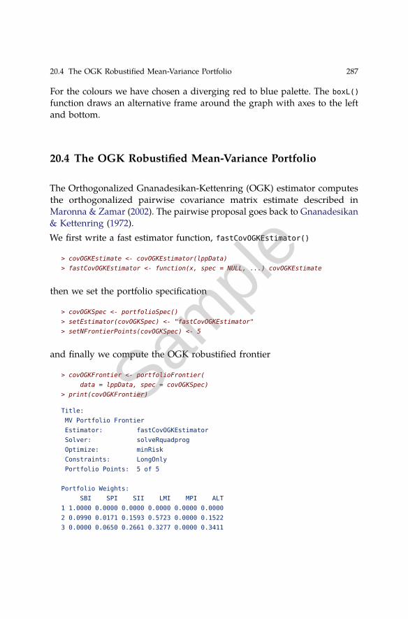
20.4 The OGK Robustified Mean-Variance Portfolio
The Orthogonalized Gnanadesikan-Kettenring (OGK) estimator computesthe orthogonalized pairwise covariance matrix estimate described inMaronna & Zamar (2002). The pairwise proposal goes back to Gnanadesikan& Kettenring (1972).We first write a fast estimator function, fastCovOGKEstimator()
> covOGKEstimate <- covOGKEstimator(lppData)
> fastCovOGKEstimator <- function(x, spec = NULL, ...) covOGKEstimate
then we set the portfolio specification
> covOGKSpec <- portfolioSpec()
> setEstimator(covOGKSpec) <- "fastCovOGKEstimator"
> setNFrontierPoints(covOGKSpec) <- 5
and finally we compute the OGK robustified frontier
> covOGKFrontier <- portfolioFrontier(
data = lppData, spec = covOGKSpec)
> print(covOGKFrontier)
Title:
MV Portfolio Frontier
Estimator: fastCovOGKEstimator
Solver: solveRquadprog
Optimize: minRisk
Constraints: LongOnly
Portfolio Points: 5 of 5
Portfolio Weights:
SBI SPI SII LMI MPI ALT
1 1.0000 0.0000 0.0000 0.0000 0.0000 0.0000
2 0.0990 0.0171 0.1593 0.5723 0.0000 0.1522
3 0.0000 0.0650 0.2661 0.3277 0.0000 0.3411
Sample
288 20 Robust Portfolios and Covariance Estimation0.
00.
40.
8 SBISPISIILMIMPIALT
0.0
0.4
0.8
0.126 0.148 0.325 0.534
4.07e−05 0.0542 0.0813
Target Risk
Target Return
Wei
ght
Weights MVE
0.00
0.04
0.08 SBI
SPISIILMIMPIALT
0.00
0.04
0.08
0.126 0.148 0.325 0.534
4.07e−05 0.0542 0.0813
Target Risk
Target Return
Wei
ghte
d R
etur
n
Weighted Returns
0.0
0.4
0.8
SBISPISIILMIMPIALT
0.0
0.4
0.8
0.126 0.148 0.325 0.534
4.07e−05 0.0542 0.0813
Target Risk
Target Return
Cov
Ris
k B
udge
ts
Cov Risk Budgets
0.0
0.4
0.8 SBI
SPISIILMIMPIALT
0.0
0.4
0.8
0.126 0.15 0.329 0.54
4.07e−05 0.0542 0.0813
Target Risk
Target ReturnW
eigh
t
Weights MCD
0.00
0.04
0.08 SBI
SPISIILMIMPIALT
0.00
0.04
0.08
0.126 0.15 0.329 0.54
4.07e−05 0.0542 0.0813
Target Risk
Target Return
Wei
ghte
d R
etur
n
Weighted Returns
0.0
0.4
0.8
SBISPISIILMIMPIALT
0.0
0.4
0.8
0.126 0.15 0.329 0.54
4.07e−05 0.0542 0.0813
Target Risk
Target Return
Cov
Ris
k B
udge
ts
Cov Risk Budgets
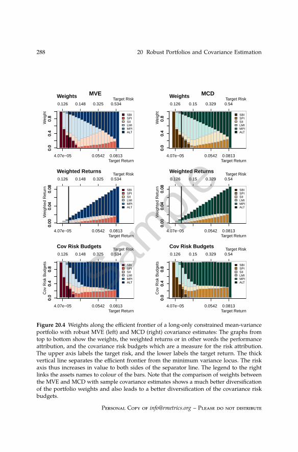
Figure 20.4 Weights along the efficient frontier of a long-only constrained mean-varianceportfolio with robust MVE (left) and MCD (right) covariance estimates: The graphs fromtop to bottom show the weights, the weighted returns or in other words the performanceattribution, and the covariance risk budgets which are a measure for the risk attribution.The upper axis labels the target risk, and the lower labels the target return. The thickvertical line separates the efficient frontier from the minimum variance locus. The riskaxis thus increases in value to both sides of the separator line. The legend to the rightlinks the assets names to colour of the bars. Note that the comparison of weights betweenthe MVE and MCD with sample covariance estimates shows a much better diversificationof the portfolio weights and also leads to a better diversification of the covariance riskbudgets.
Personal Copy of [email protected] – Please do not distribute
Sample
20.4 The OGK Robustified Mean-Variance Portfolio 289
4 0.0000 0.1179 0.3433 0.0000 0.0000 0.5388
5 0.0000 0.0000 0.0000 0.0000 0.0000 1.0000
Covariance Risk Budgets:
SBI SPI SII LMI MPI ALT
1 1.0000 0.0000 0.0000 0.0000 0.0000 0.0000
2 0.0347 0.0583 0.1827 0.2605 0.0000 0.4639
3 0.0000 0.1540 0.1329 -0.0089 0.0000 0.7221
4 0.0000 0.1790 0.0895 0.0000 0.0000 0.7315
5 0.0000 0.0000 0.0000 0.0000 0.0000 1.0000
Target Return and Risks:
mean mu Cov Sigma CVaR VaR
1 0.0000 0.0000 0.1261 0.1270 0.2758 0.2177
2 0.0215 0.0215 0.1223 0.1197 0.2419 0.1741
3 0.0429 0.0429 0.2460 0.2222 0.5450 0.3418
4 0.0643 0.0643 0.3976 0.3532 0.9175 0.5523
5 0.0858 0.0858 0.5684 0.5236 1.3343 0.8978
Description:
Mon May 4 12:04:56 2009 by user: Rmetrics
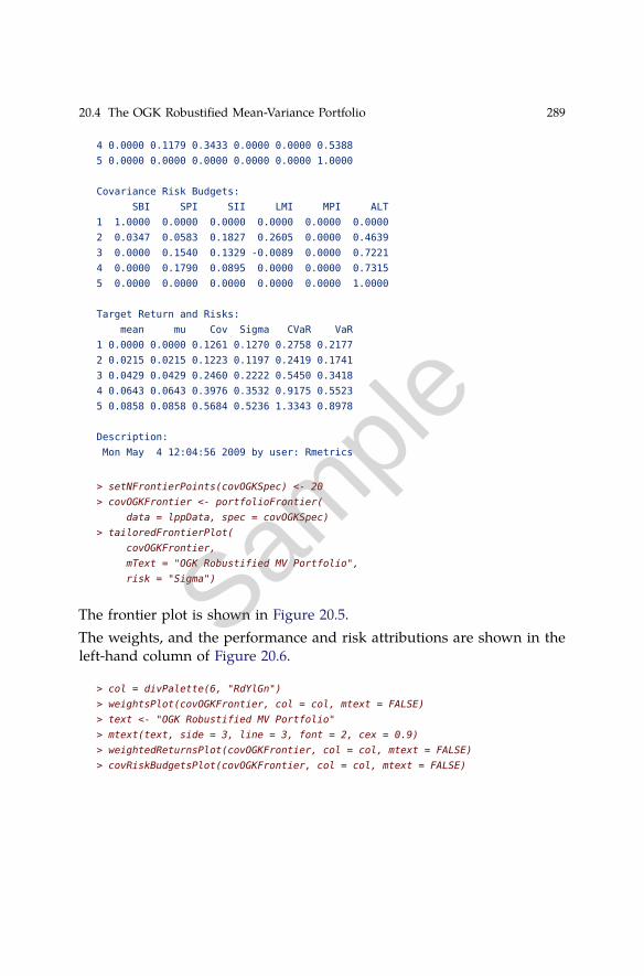
> setNFrontierPoints(covOGKSpec) <- 20
> covOGKFrontier <- portfolioFrontier(
data = lppData, spec = covOGKSpec)
> tailoredFrontierPlot(
covOGKFrontier,
mText = "OGK Robustified MV Portfolio",
risk = "Sigma")
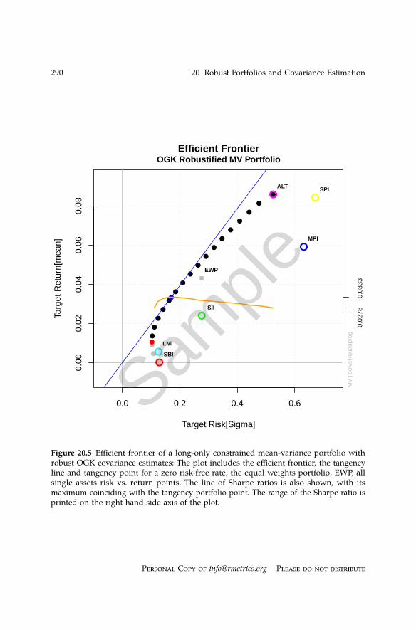
The frontier plot is shown in Figure 20.5.The weights, and the performance and risk attributions are shown in theleft-hand column of Figure 20.6.
> col = divPalette(6, "RdYlGn")
> weightsPlot(covOGKFrontier, col = col, mtext = FALSE)
> text <- "OGK Robustified MV Portfolio"
> mtext(text, side = 3, line = 3, font = 2, cex = 0.9)
> weightedReturnsPlot(covOGKFrontier, col = col, mtext = FALSE)
> covRiskBudgetsPlot(covOGKFrontier, col = col, mtext = FALSE)
Sample
290 20 Robust Portfolios and Covariance Estimation
0.0 0.2 0.4 0.6
0.00
0.02
0.04
0.06
0.08
●
●
●
●
●
●
●
●
●
●
●
●
●
●
●
●
●
●
●
●M
V |
solv
eRqu
adpr
og
Efficient Frontier
Target Risk[Sigma]
Targ
et R
etur
n[m
ean]
OGK Robustified MV Portfolio
●
●
EWP
●
●
●
●
●
●
SBI
SPI
SII
LMI
MPI
ALT
0.02
78
0.0
333
Figure 20.5 Efficient frontier of a long-only constrained mean-variance portfolio withrobust OGK covariance estimates: The plot includes the efficient frontier, the tangencyline and tangency point for a zero risk-free rate, the equal weights portfolio, EWP, allsingle assets risk vs. return points. The line of Sharpe ratios is also shown, with itsmaximum coinciding with the tangency portfolio point. The range of the Sharpe ratio isprinted on the right hand side axis of the plot.
Personal Copy of [email protected] – Please do not distribute
Sample
20.4 The OGK Robustified Mean-Variance Portfolio 2910.
00.
40.
8 SBISPISIILMIMPIALT
0.0
0.4
0.8
0.126 0.148 0.325 0.535
4.07e−05 0.0542 0.0813
Target Risk
Target Return
Wei
ght
Weights OGK
0.00
0.04
0.08 SBI
SPISIILMIMPIALT
0.00
0.04
0.08
0.126 0.148 0.325 0.535
4.07e−05 0.0542 0.0813
Target Risk
Target Return
Wei
ghte
d R
etur
n
Weighted Returns
0.0
0.4
0.8
SBISPISIILMIMPIALT
0.0
0.4
0.8
0.126 0.148 0.325 0.535
4.07e−05 0.0542 0.0813
Target Risk
Target Return
Cov
Ris
k B
udge
ts
Cov Risk Budgets
0.0
0.4
0.8 SBI
SPISIILMIMPIALT
0.0
0.4
0.8
0.126 0.15 0.329 0.54
4.07e−05 0.0542 0.0813
Target Risk
Target ReturnW
eigh
t
Weights MCD
0.00
0.04
0.08 SBI
SPISIILMIMPIALT
0.00
0.04
0.08
0.126 0.15 0.329 0.54
4.07e−05 0.0542 0.0813
Target Risk
Target Return
Wei
ghte
d R
etur
n
Weighted Returns
0.0
0.4
0.8
SBISPISIILMIMPIALT
0.0
0.4
0.8
0.126 0.15 0.329 0.54
4.07e−05 0.0542 0.0813
Target Risk
Target Return
Cov
Ris
k B
udge
ts
Cov Risk Budgets
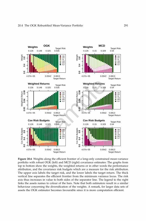
Figure 20.6 Weights along the efficient frontier of a long-only constrained mean-varianceportfolio with robust OGK (left) and MCD (right) covariance estimates: The graphs fromtop to bottom show the weights, the weighted returns or in other words the performanceattribution, and the covariance risk budgets which are a measure for the risk attribution.The upper axis labels the target risk, and the lower labels the target return. The thickvertical line separates the efficient frontier from the minimum variance locus. The riskaxis thus increases in value to both sides of the separator line. The legend to the rightlinks the assets names to colour of the bars. Note that both estimators result in a similarbehaviour concerning the diversification of the weights. A remark, for larger data sets ofassets the OGK estimator becomes favourable since it is more computation efficient.
Sample
292 20 Robust Portfolios and Covariance Estimation
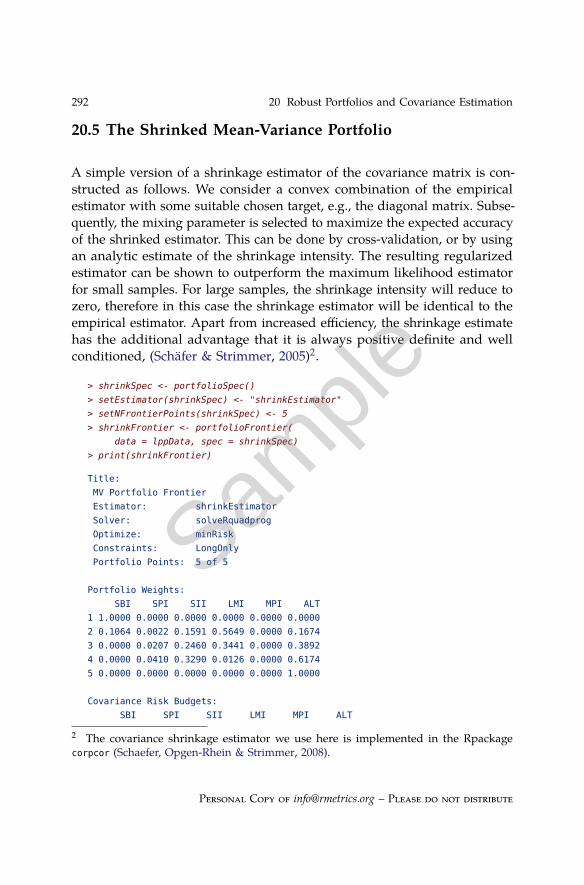
20.5 The Shrinked Mean-Variance Portfolio
A simple version of a shrinkage estimator of the covariance matrix is con-structed as follows. We consider a convex combination of the empiricalestimator with some suitable chosen target, e.g., the diagonal matrix. Subse-quently, the mixing parameter is selected to maximize the expected accuracyof the shrinked estimator. This can be done by cross-validation, or by usingan analytic estimate of the shrinkage intensity. The resulting regularizedestimator can be shown to outperform the maximum likelihood estimatorfor small samples. For large samples, the shrinkage intensity will reduce tozero, therefore in this case the shrinkage estimator will be identical to theempirical estimator. Apart from increased efficiency, the shrinkage estimatehas the additional advantage that it is always positive definite and wellconditioned, (Schäfer & Strimmer, 2005)2.
> shrinkSpec <- portfolioSpec()
> setEstimator(shrinkSpec) <- "shrinkEstimator"
> setNFrontierPoints(shrinkSpec) <- 5
> shrinkFrontier <- portfolioFrontier(
data = lppData, spec = shrinkSpec)
> print(shrinkFrontier)
Title:
MV Portfolio Frontier
Estimator: shrinkEstimator
Solver: solveRquadprog
Optimize: minRisk
Constraints: LongOnly
Portfolio Points: 5 of 5
Portfolio Weights:
SBI SPI SII LMI MPI ALT
1 1.0000 0.0000 0.0000 0.0000 0.0000 0.0000
2 0.1064 0.0022 0.1591 0.5649 0.0000 0.1674
3 0.0000 0.0207 0.2460 0.3441 0.0000 0.3892
4 0.0000 0.0410 0.3290 0.0126 0.0000 0.6174
5 0.0000 0.0000 0.0000 0.0000 0.0000 1.0000
Covariance Risk Budgets:
SBI SPI SII LMI MPI ALT
2 The covariance shrinkage estimator we use here is implemented in the Rpackagecorpcor (Schaefer, Opgen-Rhein & Strimmer, 2008).
Personal Copy of [email protected] – Please do not distribute
Sample
20.6 How to Write Your Own Covariance Estimator 293
1 1.0000 0.0000 0.0000 0.0000 0.0000 0.0000
2 0.0378 0.0070 0.1812 0.2553 0.0000 0.5188
3 0.0000 0.0455 0.1154 -0.0094 0.0000 0.8485
4 0.0000 0.0576 0.0823 -0.0009 0.0000 0.8610
5 0.0000 0.0000 0.0000 0.0000 0.0000 1.0000
Target Return and Risks:
mean mu Cov Sigma CVaR VaR
1 0.0000 0.0000 0.1261 0.1449 0.2758 0.2177
2 0.0215 0.0215 0.1219 0.1283 0.2386 0.1772
3 0.0429 0.0429 0.2440 0.2430 0.5328 0.3386
4 0.0643 0.0643 0.3941 0.3920 0.8923 0.5868
5 0.0858 0.0858 0.5684 0.5656 1.3343 0.8978
Description:
Mon May 4 12:04:59 2009 by user: Rmetrics
The results are shown in Figure 20.7 and Figure 20.8.
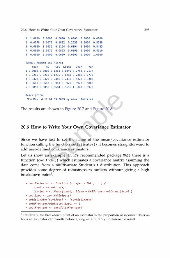
20.6 How to Write Your Own Covariance Estimator
Since we have just to set the name of the mean/covariance estimatorfunction calling the function setEstimator() it becomes straightforward toadd user-defined covariance estimators.Let us show an example. In R’s recommended package MASS there is afunction (cov.trob()) which estimates a covariance matrix assuming thedata come from a multivariate Student’s t distribution. This approachprovides some degree of robustness to outliers without giving a highbreakdown point3.
> covtEstimator <- function (x, spec = NULL, ...) {
x.mat = as.matrix(x)
list(mu = colMeans(x.mat), Sigma = MASS::cov.trob(x.mat)$cov) }
> covtSpec <- portfolioSpec()
> setEstimator(covtSpec) <- "covtEstimator"
> setNFrontierPoints(covtSpec) <- 5
> covtFrontier <- portfolioFrontier(
3 Intuitively, the breakdown point of an estimator is the proportion of incorrect observa-tions an estimator can handle before giving an arbitrarily unreasonable result
Sample
294 20 Robust Portfolios and Covariance Estimation
0.0 0.2 0.4 0.6 0.8
0.00
0.02
0.04
0.06
0.08
●
●
●
●
●
●
●
●
●
●
●
●
●
●
●
●
●
●
●
●
MV
| so
lveR
quad
prog
Efficient Frontier
Target Risk[Sigma]
Targ
et R
etur
n[m
ean]
Shrinked MV Portfolio
●
●
EWP
●
●
●
●
●
●
SBI
SPI
SII
LMI
MPI
ALT
0.02
64
0.0
316
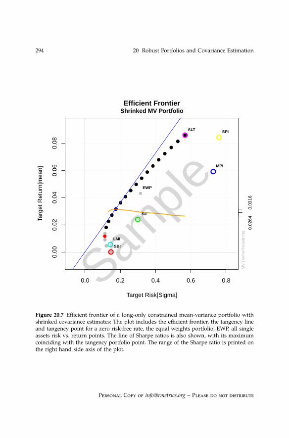
Figure 20.7 Efficient frontier of a long-only constrained mean-variance portfolio withshrinked covariance estimates: The plot includes the efficient frontier, the tangency lineand tangency point for a zero risk-free rate, the equal weights portfolio, EWP, all singleassets risk vs. return points. The line of Sharpe ratios is also shown, with its maximumcoinciding with the tangency portfolio point. The range of the Sharpe ratio is printed onthe right hand side axis of the plot.
Personal Copy of [email protected] – Please do not distribute
Sample
20.6 How to Write Your Own Covariance Estimator 2950.
00.
40.
8 SBISPISIILMIMPIALT
0.0
0.4
0.8
0.126 0.147 0.322 0.529
4.07e−05 0.0271 0.0542 0.0813
Target Risk
Target Return
Wei
ght
Weights Shrinked MV Portfolio
0.00
0.04
0.08 SBI
SPISIILMIMPIALT
0.00
0.04
0.08
0.126 0.147 0.322 0.529
4.07e−05 0.0271 0.0542 0.0813
Target Risk
Target Return
Wei
ghte
d R
etur
n
Weighted Returns
0.0
0.4
0.8
SBISPISIILMIMPIALT
0.0
0.4
0.8
0.126 0.147 0.322 0.529
4.07e−05 0.0271 0.0542 0.0813
Target Risk
Target Return
Cov
Ris
k B
udge
ts
Cov Risk Budgets
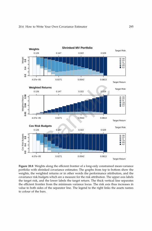
Figure 20.8 Weights along the efficient frontier of a long-only constrained mean-varianceportfolio with shrinked covariance estimates: The graphs from top to bottom show theweights, the weighted returns or in other words the performance attribution, and thecovariance risk budgets which are a measure for the risk attribution. The upper axis labelsthe target risk, and the lower labels the target return. The thick vertical line separatesthe efficient frontier from the minimum variance locus. The risk axis thus increases invalue to both sides of the separator line. The legend to the right links the assets namesto colour of the bars.
Sample
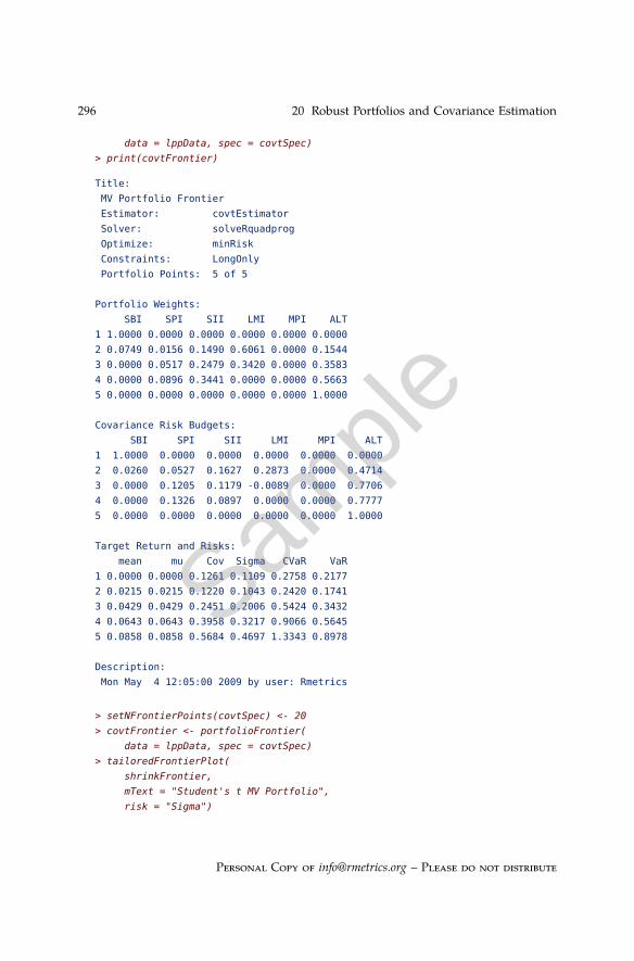
296 20 Robust Portfolios and Covariance Estimation
data = lppData, spec = covtSpec)
> print(covtFrontier)
Title:
MV Portfolio Frontier
Estimator: covtEstimator
Solver: solveRquadprog
Optimize: minRisk
Constraints: LongOnly
Portfolio Points: 5 of 5
Portfolio Weights:
SBI SPI SII LMI MPI ALT
1 1.0000 0.0000 0.0000 0.0000 0.0000 0.0000
2 0.0749 0.0156 0.1490 0.6061 0.0000 0.1544
3 0.0000 0.0517 0.2479 0.3420 0.0000 0.3583
4 0.0000 0.0896 0.3441 0.0000 0.0000 0.5663
5 0.0000 0.0000 0.0000 0.0000 0.0000 1.0000
Covariance Risk Budgets:
SBI SPI SII LMI MPI ALT
1 1.0000 0.0000 0.0000 0.0000 0.0000 0.0000
2 0.0260 0.0527 0.1627 0.2873 0.0000 0.4714
3 0.0000 0.1205 0.1179 -0.0089 0.0000 0.7706
4 0.0000 0.1326 0.0897 0.0000 0.0000 0.7777
5 0.0000 0.0000 0.0000 0.0000 0.0000 1.0000
Target Return and Risks:
mean mu Cov Sigma CVaR VaR
1 0.0000 0.0000 0.1261 0.1109 0.2758 0.2177
2 0.0215 0.0215 0.1220 0.1043 0.2420 0.1741
3 0.0429 0.0429 0.2451 0.2006 0.5424 0.3432
4 0.0643 0.0643 0.3958 0.3217 0.9066 0.5645
5 0.0858 0.0858 0.5684 0.4697 1.3343 0.8978
Description:
Mon May 4 12:05:00 2009 by user: Rmetrics
> setNFrontierPoints(covtSpec) <- 20
> covtFrontier <- portfolioFrontier(
data = lppData, spec = covtSpec)
> tailoredFrontierPlot(
shrinkFrontier,
mText = "Student's t MV Portfolio",
risk = "Sigma")
Personal Copy of [email protected] – Please do not distribute
Sample

20.6 How to Write Your Own Covariance Estimator 297
The frontier plot is shown in Figure 20.9. The weights and related plots arecomputed in the usual way, and presented in Figure 20.10.
> weightsPlot(covtFrontier, mtext = FALSE)
> text <- "Student's t"
> mtext(text, side = 3, line = 3, font = 2, cex = 0.9)
> weightedReturnsPlot(covtFrontier, mtext = FALSE)
> covRiskBudgetsPlot(covtFrontier, mtext = FALSE)
Sample
298 20 Robust Portfolios and Covariance Estimation
0.0 0.2 0.4 0.6
0.00
0.02
0.04
0.06
0.08
●
●
●
●
●
●
●
●
●
●
●
●
●
●
●
●
●
●
●
●M
V |
solv
eRqu
adpr
og
Efficient Frontier
Target Risk[Sigma]
Targ
et R
etur
n[m
ean]
Student's t MV Portfolio
●
●
EWP
●
●
●
●
●
●
SBI
SPI
SII
LMI
MPI
ALT
0.02
56
0.0
309
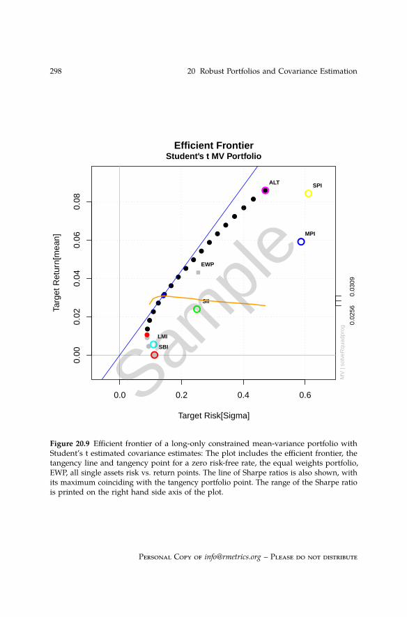
Figure 20.9 Efficient frontier of a long-only constrained mean-variance portfolio withStudent’s t estimated covariance estimates: The plot includes the efficient frontier, thetangency line and tangency point for a zero risk-free rate, the equal weights portfolio,EWP, all single assets risk vs. return points. The line of Sharpe ratios is also shown, withits maximum coinciding with the tangency portfolio point. The range of the Sharpe ratiois printed on the right hand side axis of the plot.
Personal Copy of [email protected] – Please do not distribute
Sample
20.6 How to Write Your Own Covariance Estimator 2990.
00.
40.
8 SBISPISIILMIMPIALT
0.0
0.4
0.8
0.126 0.148 0.323 0.532
4.07e−05 0.0271 0.0542 0.0813
Target Risk
Target Return
Wei
ght
Weights Student's t
0.00
0.04
0.08 SBI
SPISIILMIMPIALT
0.00
0.04
0.08
0.126 0.148 0.323 0.532
4.07e−05 0.0271 0.0542 0.0813
Target Risk
Target Return
Wei
ghte
d R
etur
n
Weighted Returns
0.0
0.4
0.8
SBISPISIILMIMPIALT
0.0
0.4
0.8
0.126 0.148 0.323 0.532
4.07e−05 0.0271 0.0542 0.0813
Target Risk
Target Return
Cov
Ris
k B
udge
ts
Cov Risk Budgets
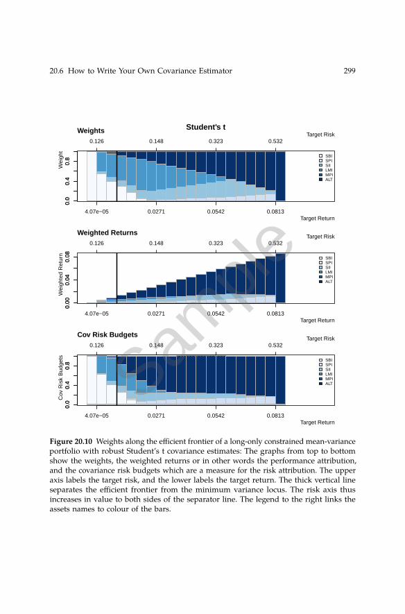
Figure 20.10 Weights along the efficient frontier of a long-only constrained mean-varianceportfolio with robust Student’s t covariance estimates: The graphs from top to bottomshow the weights, the weighted returns or in other words the performance attribution,and the covariance risk budgets which are a measure for the risk attribution. The upperaxis labels the target risk, and the lower labels the target return. The thick vertical lineseparates the efficient frontier from the minimum variance locus. The risk axis thusincreases in value to both sides of the separator line. The legend to the right links theassets names to colour of the bars.
Sample
Appendix A
Packages Required for this ebook
Required R package(s):
> library(fPortfolio)
In the following we briefly describe the packages required for this ebook.There are two major packages named fPortfolio and fPortfolioBacktest.The first package, fPortfolio, is the basic package which allows us to modelmean-variance and mean-CVaR portfolios with linear constraints and toanalyze the data sets of assets used in the portfolios. The second package,fPortfolioBacktest, adds additional functionality, including backtestingfunctions over rolling windows.
Rmetrics Package: fPortfolio
fPortfolio (Würtz & Chalabi, 2009a) contains the R functions for solvingmean-variance and mean-CVaR portfolio problems with linear constraints.The package depends on the contributed R packages quadprog (Weingessel,2004) for quadratic programming problems and Rglpk (Theussl & Hornik,2009) with the appropriate solvers for quadratic and linear programmingproblems.
> listDescription(fPortfolio)
fPortfolio Description:
389
Sample

A Packages Required for this ebook 397
URL: http://www.rmetrics.org
Built: R 2.9.0; ; 2009-04-23 09:48:16 UTC; unix
Sample
About the Authors
Diethelm Würtz is private lecturer at the Institute for Theoretical Physics,ITP, and for the Curriculum Computational Science and Engineering, CSE,at the Swiss Federal Institute of Technology in Zurich. He teaches Econo-physics at ITP and supervises seminars in Financial Engineering at CSE.Diethelm is senior partner of Finance Online, an ETH spin-off company inZurich, and co-founder of the Rmetrics Association.
Yohan Chalabi has a master in Physics from the Swiss Federal Institute ofTechnology in Lausanne. He is now a PhD student in the Econophysicsgroup at ETH Zurich at the Institute for Theoretical Physics. Yohan is aco-maintainer of the Rmetrics packages.
William Chen has a master in statistics from University of Auckland inNew Zealand. In the summer of 2008, he did a Student Internship in theEconophysics group at ETH Zurich at the Institute for Theoretical Physics.During his three months internship, William contributed to the portfoliobacktest package.
Andrew Ellis read neuroscience and mathematics at the University inZurich. He is working for Finance Online and is currently doing a 6 monthStudent Internship in the Econophysics group at ETH Zurich at the Institutefor Theoretical Physics. Andrew is working on the Rmetrics documentationproject and co-authored this ebook on portfolio optimization with Rmetrics.
411
Sample

Sample


![Package ‘fExtremes’ · Title Rmetrics - Modelling Extreme Events in Finance Date 2017-11-12 Version 3042.82 Author Diethelm Wuertz [aut], Tobias Setz [cre], Yohan Chalabi [ctb]](https://img.pdfslide.us/doc/110x75/606792fe8cbc3818953baab6/package-afextremesa-title-rmetrics-modelling-extreme-events-in-finance-date.jpg)