Embed Size (px)
Citation preview
Quantile Regression: A Gentle Introduction
Roger Koenker
University of Illinois, Urbana-Champaign
5th RMetrics Workshop, Meielisalp: 28 June 2011
Roger Koenker (UIUC) Introduction Meielisalp: 28.6.2011 1 / 58

Overview of the Course
Some Basics: What, Why and How?
Inference and Quantile Treatment Effects
Nonparametric Quantile Regression
Quantile Autoregression
Risk Assessment and Choquet Portfolios
Course outline, lecture slides, an R FAQ, and even some proposed exercisescan all be found at:
http://www.econ.uiuc.edu/~roger/courses/RMetrics.
A somewhat more extensive set of lecture slides can be found at:
http://www.econ.uiuc.edu/~roger/courses/LSE.
Roger Koenker (UIUC) Introduction Meielisalp: 28.6.2011 2 / 58

Boxplots of CEO Pay
firm market value in billions
annu
al c
ompe
nsat
ion
in m
illio
ns
●
●
●
●●
0.1 1 10 100
0.1
110
100
** * * * *
** *
*
++ + + + +
++
+
+
Roger Koenker (UIUC) Introduction Meielisalp: 28.6.2011 3 / 58
Motivation
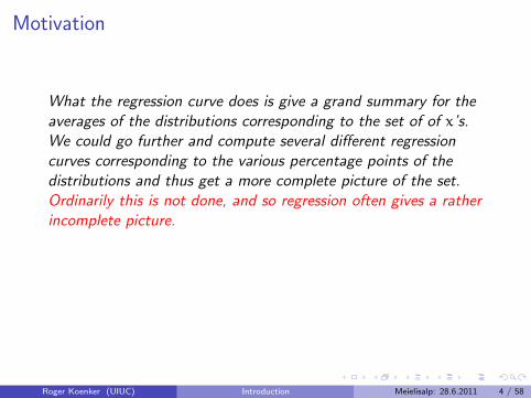
What the regression curve does is give a grand summary for theaverages of the distributions corresponding to the set of of x’s.We could go further and compute several different regressioncurves corresponding to the various percentage points of thedistributions and thus get a more complete picture of the set.
Ordinarily this is not done, and so regression often gives a ratherincomplete picture. Just as the mean gives an incomplete pictureof a single distribution, so the regression curve gives acorrespondingly incomplete picture for a set of distributions.
Mosteller and Tukey (1977)
Roger Koenker (UIUC) Introduction Meielisalp: 28.6.2011 4 / 58
Motivation
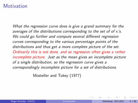
What the regression curve does is give a grand summary for theaverages of the distributions corresponding to the set of of x’s.We could go further and compute several different regressioncurves corresponding to the various percentage points of thedistributions and thus get a more complete picture of the set.Ordinarily this is not done, and so regression often gives a ratherincomplete picture.
Just as the mean gives an incomplete pictureof a single distribution, so the regression curve gives acorrespondingly incomplete picture for a set of distributions.
Mosteller and Tukey (1977)
Roger Koenker (UIUC) Introduction Meielisalp: 28.6.2011 4 / 58
Motivation
What the regression curve does is give a grand summary for theaverages of the distributions corresponding to the set of of x’s.We could go further and compute several different regressioncurves corresponding to the various percentage points of thedistributions and thus get a more complete picture of the set.Ordinarily this is not done, and so regression often gives a ratherincomplete picture. Just as the mean gives an incomplete pictureof a single distribution, so the regression curve gives acorrespondingly incomplete picture for a set of distributions.
Mosteller and Tukey (1977)
Roger Koenker (UIUC) Introduction Meielisalp: 28.6.2011 4 / 58

Motivation
Francis Galton in a famous passage defending the “charms of statistics”against its many detractors, chided his statistical colleagues
[who] limited their inquiries to Averages, and do not seem torevel in more comprehensive views. Their souls seem as dull tothe charm of variety as that of a native of one of our flat Englishcounties, whose retrospect of Switzerland was that, if themountains could be thrown into its lakes, two nuisances wouldbe got rid of at once. Natural Inheritance, 1889
Roger Koenker (UIUC) Introduction Meielisalp: 28.6.2011 5 / 58
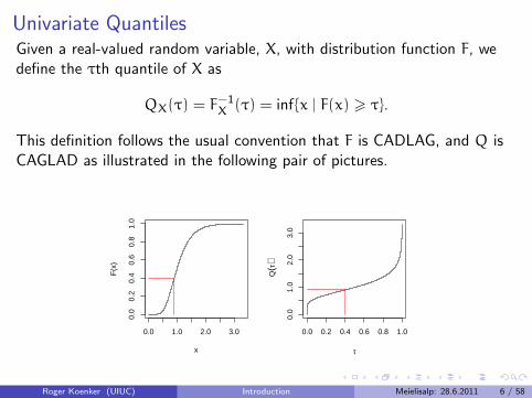
Univariate QuantilesGiven a real-valued random variable, X, with distribution function F, wedefine the τth quantile of X as
QX(τ) = F−1X (τ) = inf{x | F(x) > τ}.
This definition follows the usual convention that F is CADLAG, and Q isCAGLAD as illustrated in the following pair of pictures.
0.0 1.0 2.0 3.0
0.0
0.2
0.4
0.6
0.8
1.0
x
F(x
)
0.0 0.2 0.4 0.6 0.8 1.0
0.0
1.0
2.0
3.0
τ
Q(τ
)
Roger Koenker (UIUC) Introduction Meielisalp: 28.6.2011 6 / 58
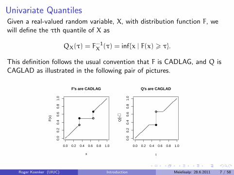
Univariate QuantilesGiven a real-valued random variable, X, with distribution function F, wewill define the τth quantile of X as
QX(τ) = F−1X (τ) = inf{x | F(x) > τ}.
This definition follows the usual convention that F is CADLAG, and Q isCAGLAD as illustrated in the following pair of pictures.
0.0 0.2 0.4 0.6 0.8 1.0
0.0
0.2
0.4
0.6
0.8
1.0
x
F(x
)
●
● ●
●
F's are CADLAG
0.0 0.2 0.4 0.6 0.8 1.0
0.0
0.2
0.4
0.6
0.8
1.0
τ
Q(τ
)●
●
Q's are CAGLAD
Roger Koenker (UIUC) Introduction Meielisalp: 28.6.2011 7 / 58
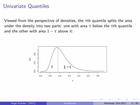
Univariate Quantiles
Viewed from the perspective of densities, the τth quantile splits the areaunder the density into two parts: one with area τ below the τth quantileand the other with area 1 − τ above it:
0.0 0.5 1.0 1.5 2.0 2.5 3.0
0.0
0.4
0.8
x
f(x)
τ 1 − τ
Roger Koenker (UIUC) Introduction Meielisalp: 28.6.2011 8 / 58
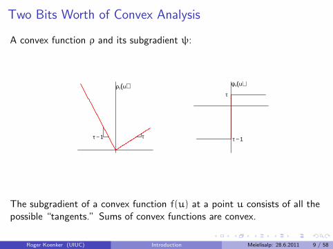
Two Bits Worth of Convex Analysis
A convex function ρ and its subgradient ψ:
ττ − 1
ρτ(u)τ
τ − 1
ψτ(u)
The subgradient of a convex function f(u) at a point u consists of all thepossible “tangents.” Sums of convex functions are convex.
Roger Koenker (UIUC) Introduction Meielisalp: 28.6.2011 9 / 58
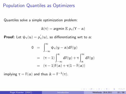
Population Quantiles as Optimizers
Quantiles solve a simple optimization problem:
α(τ) = argmin E ρτ(Y − α)
Proof: Let ψτ(u) = ρ′τ(u), so differentiating wrt to α:
0 =
∫∞−∞ψτ(y− α)dF(y)
= (τ− 1)
∫α−∞ dF(y) + τ
∫∞αdF(y)
= (τ− 1)F(α) + τ(1 − F(α))
implying τ = F(α) and thus α = F−1(τ).
Roger Koenker (UIUC) Introduction Meielisalp: 28.6.2011 10 / 58
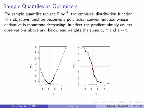
Sample Quantiles as Optimizers
For sample quantiles replace F by F, the empirical distribution function.The objective function becomes a polyhedral convex function whosederivative is monotone decreasing, in effect the gradient simply countsobservations above and below and weights the sums by τ and 1 − τ.
−2 0 2 4
2030
4050
6070
80
x
R(x
)
●
●
●
●
●●
●●●●
●●
●●●●●●●●●●
●
●●
●
●●
●
●
●
−2 0 2 4
−15
−10
−5
05
1015
x
R'(x
)
●
●
●
●
●
●
●
●
●
●
●
●
●
●
●
●
●
●
●
●
●
●
●
●
●
●
●
●
●
●
●
Roger Koenker (UIUC) Introduction Meielisalp: 28.6.2011 11 / 58
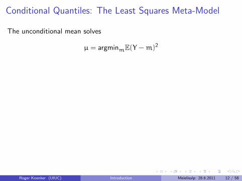
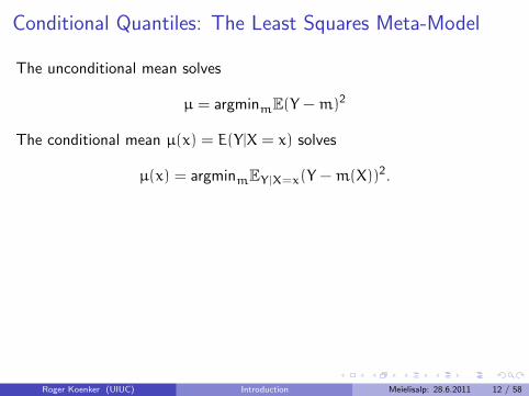
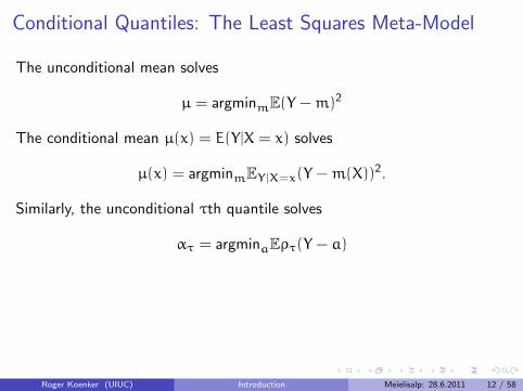
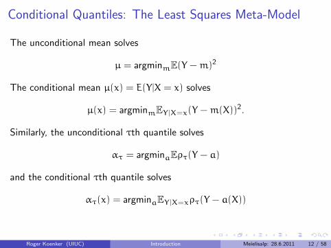
Conditional Quantiles: The Least Squares Meta-Model
The unconditional mean solves
µ = argminmE(Y −m)2
The conditional mean µ(x) = E(Y|X = x) solves
µ(x) = argminmEY|X=x(Y −m(X))2.
Similarly, the unconditional τth quantile solves
ατ = argminaEρτ(Y − a)
and the conditional τth quantile solves
ατ(x) = argminaEY|X=xρτ(Y − a(X))
Roger Koenker (UIUC) Introduction Meielisalp: 28.6.2011 12 / 58
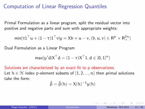
Computation of Linear Regression Quantiles
Primal Formulation as a linear program, split the residual vector intopositive and negative parts and sum with appropriate weights:
min{τ1>u+ (1 − τ)1>v|y = Xb+ u− v, (b,u, v) ∈ |Rp × |R2n+ }
Dual Formulation as a Linear Program
max{y ′d|X>d = (1 − τ)X>1,d ∈ [0, 1]n}
Solutions are characterized by an exact fit to p observations.Let h ∈ H index p-element subsets of {1, 2, ...,n} then primal solutionstake the form:
β = β(h) = X(h)−1y(h)
Roger Koenker (UIUC) Introduction Meielisalp: 28.6.2011 13 / 58
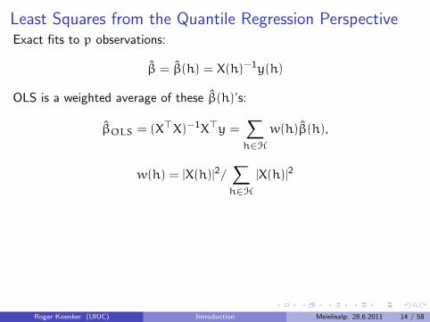
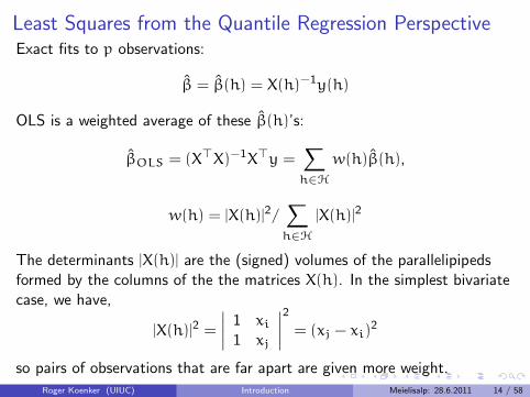
Least Squares from the Quantile Regression PerspectiveExact fits to p observations:
β = β(h) = X(h)−1y(h)
OLS is a weighted average of these β(h)’s:
βOLS = (X>X)−1X>y =∑h∈H
w(h)β(h),
w(h) = |X(h)|2/∑h∈H
|X(h)|2
The determinants |X(h)| are the (signed) volumes of the parallelipipedsformed by the columns of the the matrices X(h). In the simplest bivariatecase, we have,
|X(h)|2 =
∣∣∣∣ 1 xi1 xj
∣∣∣∣2 = (xj − xi)2
so pairs of observations that are far apart are given more weight.
Roger Koenker (UIUC) Introduction Meielisalp: 28.6.2011 14 / 58
Quantile Regression: The Movie
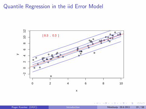
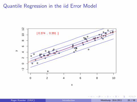
Bivariate linear model with iid Student t errors
Conditional quantile functions are parallel in blue
100 observations indicated in blue
Fitted quantile regression lines in red.
Intervals for τ ∈ (0, 1) for which the solution is optimal.
Roger Koenker (UIUC) Introduction Meielisalp: 28.6.2011 15 / 58

Quantile Regression in the iid Error Model
0 2 4 6 8 10
−2
02
46
810
12
x
y
●
●●
●
●
●
●
●●
●
●
●
●
●
●
● ●
●
●
●
●
●
●
●
●
●●
●
●
●
●
●
●
● ●
●
●
●
●
●
●●●
●
● ●
●
●
●
●
●
●
●
●
●
●
●
●
●
●
[ 0.069 , 0.096 ]
Roger Koenker (UIUC) Introduction Meielisalp: 28.6.2011 16 / 58

Quantile Regression in the iid Error Model
0 2 4 6 8 10
−2
02
46
810
12
x
y
●
●●
●
●
●
●
●●
●
●
●
●
●
●
● ●
●
●
●
●
●
●
●
●
●●
●
●
●
●
●
●
● ●
●
●
●
●
●
●●●
●
● ●
●
●
●
●
●
●
●
●
●
●
●
●
●
●
[ 0.138 , 0.151 ]
Roger Koenker (UIUC) Introduction Meielisalp: 28.6.2011 17 / 58

Quantile Regression in the iid Error Model
0 2 4 6 8 10
−2
02
46
810
12
x
y
●
●●
●
●
●
●
●●
●
●
●
●
●
●
● ●
●
●
●
●
●
●
●
●
●●
●
●
●
●
●
●
● ●
●
●
●
●
●
●●●
●
● ●
●
●
●
●
●
●
●
●
●
●
●
●
●
●
[ 0.231 , 0.24 ]
Roger Koenker (UIUC) Introduction Meielisalp: 28.6.2011 18 / 58
Quantile Regression in the iid Error Model
0 2 4 6 8 10
−2
02
46
810
12
x
y
●
●●
●
●
●
●
●●
●
●
●
●
●
●
● ●
●
●
●
●
●
●
●
●
●●
●
●
●
●
●
●
● ●
●
●
●
●
●
●●●
●
● ●
●
●
●
●
●
●
●
●
●
●
●
●
●
●
[ 0.3 , 0.3 ]
Roger Koenker (UIUC) Introduction Meielisalp: 28.6.2011 19 / 58
Quantile Regression in the iid Error Model
0 2 4 6 8 10
−2
02
46
810
12
x
y
●
●●
●
●
●
●
●●
●
●
●
●
●
●
● ●
●
●
●
●
●
●
●
●
●●
●
●
●
●
●
●
● ●
●
●
●
●
●
●●●
●
● ●
●
●
●
●
●
●
●
●
●
●
●
●
●
●
[ 0.374 , 0.391 ]
Roger Koenker (UIUC) Introduction Meielisalp: 28.6.2011 20 / 58

Quantile Regression in the iid Error Model
0 2 4 6 8 10
−2
02
46
810
12
x
y
●
●●
●
●
●
●
●●
●
●
●
●
●
●
● ●
●
●
●
●
●
●
●
●
●●
●
●
●
●
●
●
● ●
●
●
●
●
●
●●●
●
● ●
●
●
●
●
●
●
●
●
●
●
●
●
●
●
[ 0.462 , 0.476 ]
Roger Koenker (UIUC) Introduction Meielisalp: 28.6.2011 21 / 58

Quantile Regression in the iid Error Model
0 2 4 6 8 10
−2
02
46
810
12
x
y
●
●●
●
●
●
●
●●
●
●
●
●
●
●
● ●
●
●
●
●
●
●
●
●
●●
●
●
●
●
●
●
● ●
●
●
●
●
●
●●●
●
● ●
●
●
●
●
●
●
●
●
●
●
●
●
●
●
[ 0.549 , 0.551 ]
Roger Koenker (UIUC) Introduction Meielisalp: 28.6.2011 22 / 58

Quantile Regression in the iid Error Model
0 2 4 6 8 10
−2
02
46
810
12
x
y
●
●●
●
●
●
●
●●
●
●
●
●
●
●
● ●
●
●
●
●
●
●
●
●
●●
●
●
●
●
●
●
● ●
●
●
●
●
●
●●●
●
● ●
●
●
●
●
●
●
●
●
●
●
●
●
●
●
[ 0.619 , 0.636 ]
Roger Koenker (UIUC) Introduction Meielisalp: 28.6.2011 23 / 58

Quantile Regression in the iid Error Model
0 2 4 6 8 10
−2
02
46
810
12
x
y
●
●●
●
●
●
●
●●
●
●
●
●
●
●
● ●
●
●
●
●
●
●
●
●
●●
●
●
●
●
●
●
● ●
●
●
●
●
●
●●●
●
● ●
●
●
●
●
●
●
●
●
●
●
●
●
●
●
[ 0.704 , 0.729 ]
Roger Koenker (UIUC) Introduction Meielisalp: 28.6.2011 24 / 58

Quantile Regression in the iid Error Model
0 2 4 6 8 10
−2
02
46
810
12
x
y
●
●●
●
●
●
●
●●
●
●
●
●
●
●
● ●
●
●
●
●
●
●
●
●
●●
●
●
●
●
●
●
● ●
●
●
●
●
●
●●●
●
● ●
●
●
●
●
●
●
●
●
●
●
●
●
●
●
[ 0.768 , 0.798 ]
Roger Koenker (UIUC) Introduction Meielisalp: 28.6.2011 25 / 58

Quantile Regression in the iid Error Model
0 2 4 6 8 10
−2
02
46
810
12
x
y
●
●●
●
●
●
●
●●
●
●
●
●
●
●
● ●
●
●
●
●
●
●
●
●
●●
●
●
●
●
●
●
● ●
●
●
●
●
●
●●●
●
● ●
●
●
●
●
●
●
●
●
●
●
●
●
●
●
[ 0.919 , 0.944 ]
Roger Koenker (UIUC) Introduction Meielisalp: 28.6.2011 26 / 58
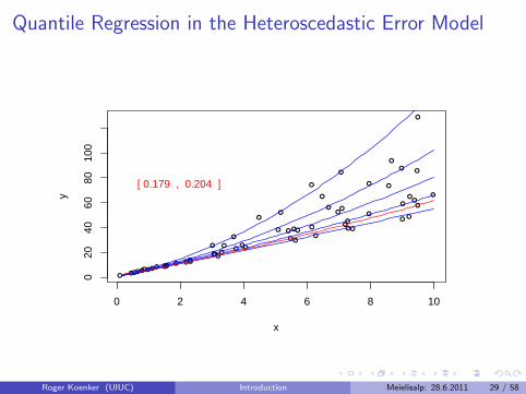
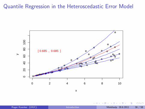
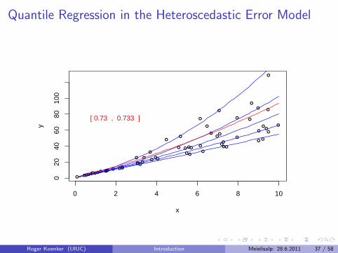
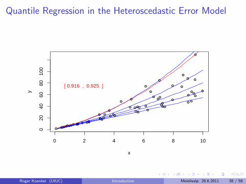
Virtual Quantile Regression II
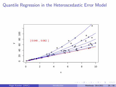
Bivariate quadratic model with Heteroscedastic χ2 errors
Conditional quantile functions drawn in blue
100 observations indicated in blue
Fitted quadratic quantile regression lines in red
Intervals of optimality for τ ∈ (0, 1).
Roger Koenker (UIUC) Introduction Meielisalp: 28.6.2011 27 / 58
Quantile Regression in the Heteroscedastic Error Model
0 2 4 6 8 10
020
4060
8010
0
x
y
●
●
●●
●
● ●
●
●
●
●
●
●
●
●●
●
●
●
●
●
●
●●
●●
●
●
●
●
●
●
●
●
●
●
●
●
●
●
●
●
●
●
●● ●
●
●
●
●
●
●
●
●
●
●
●
●
●
[ 0.048 , 0.062 ]
Roger Koenker (UIUC) Introduction Meielisalp: 28.6.2011 28 / 58
Quantile Regression in the Heteroscedastic Error Model
0 2 4 6 8 10
020
4060
8010
0
x
y
●
●
●●
●
● ●
●
●
●
●
●
●
●
●●
●
●
●
●
●
●
●●
●●
●
●
●
●
●
●
●
●
●
●
●
●
●
●
●
●
●
●
●● ●
●
●
●
●
●
●
●
●
●
●
●
●
●
[ 0.179 , 0.204 ]
Roger Koenker (UIUC) Introduction Meielisalp: 28.6.2011 29 / 58

Quantile Regression in the Heteroscedastic Error Model
0 2 4 6 8 10
020
4060
8010
0
x
y
●
●
●●
●
● ●
●
●
●
●
●
●
●
●●
●
●
●
●
●
●
●●
●●
●
●
●
●
●
●
●
●
●
●
●
●
●
●
●
●
●
●
●● ●
●
●
●
●
●
●
●
●
●
●
●
●
●
[ 0.261 , 0.261 ]
Roger Koenker (UIUC) Introduction Meielisalp: 28.6.2011 30 / 58

Quantile Regression in the Heteroscedastic Error Model
0 2 4 6 8 10
020
4060
8010
0
x
y
●
●
●●
●
● ●
●
●
●
●
●
●
●
●●
●
●
●
●
●
●
●●
●●
●
●
●
●
●
●
●
●
●
●
●
●
●
●
●
●
●
●
●● ●
●
●
●
●
●
●
●
●
●
●
●
●
●
[ 0.304 , 0.319 ]
Roger Koenker (UIUC) Introduction Meielisalp: 28.6.2011 31 / 58

Quantile Regression in the Heteroscedastic Error Model
0 2 4 6 8 10
020
4060
8010
0
x
y
●
●
●●
●
● ●
●
●
●
●
●
●
●
●●
●
●
●
●
●
●
●●
●●
●
●
●
●
●
●
●
●
●
●
●
●
●
●
●
●
●
●
●● ●
●
●
●
●
●
●
●
●
●
●
●
●
●
[ 0.414 , 0.417 ]
Roger Koenker (UIUC) Introduction Meielisalp: 28.6.2011 32 / 58

Quantile Regression in the Heteroscedastic Error Model
0 2 4 6 8 10
020
4060
8010
0
x
y
●
●
●●
●
● ●
●
●
●
●
●
●
●
●●
●
●
●
●
●
●
●●
●●
●
●
●
●
●
●
●
●
●
●
●
●
●
●
●
●
●
●
●● ●
●
●
●
●
●
●
●
●
●
●
●
●
●
[ 0.499 , 0.507 ]
Roger Koenker (UIUC) Introduction Meielisalp: 28.6.2011 33 / 58

Quantile Regression in the Heteroscedastic Error Model
0 2 4 6 8 10
020
4060
8010
0
x
y
●
●
●●
●
● ●
●
●
●
●
●
●
●
●●
●
●
●
●
●
●
●●
●●
●
●
●
●
●
●
●
●
●
●
●
●
●
●
●
●
●
●
●● ●
●
●
●
●
●
●
●
●
●
●
●
●
●
[ 0.581 , 0.582 ]
Roger Koenker (UIUC) Introduction Meielisalp: 28.6.2011 34 / 58

Quantile Regression in the Heteroscedastic Error Model
0 2 4 6 8 10
020
4060
8010
0
x
y
●
●
●●
●
● ●
●
●
●
●
●
●
●
●●
●
●
●
●
●
●
●●
●●
●
●
●
●
●
●
●
●
●
●
●
●
●
●
●
●
●
●
●● ●
●
●
●
●
●
●
●
●
●
●
●
●
●
[ 0.633 , 0.635 ]
Roger Koenker (UIUC) Introduction Meielisalp: 28.6.2011 35 / 58
Quantile Regression in the Heteroscedastic Error Model
0 2 4 6 8 10
020
4060
8010
0
x
y
●
●
●●
●
● ●
●
●
●
●
●
●
●
●●
●
●
●
●
●
●
●●
●●
●
●
●
●
●
●
●
●
●
●
●
●
●
●
●
●
●
●
●● ●
●
●
●
●
●
●
●
●
●
●
●
●
●
[ 0.685 , 0.685 ]
Roger Koenker (UIUC) Introduction Meielisalp: 28.6.2011 36 / 58
Quantile Regression in the Heteroscedastic Error Model
0 2 4 6 8 10
020
4060
8010
0
x
y
●
●
●●
●
● ●
●
●
●
●
●
●
●
●●
●
●
●
●
●
●
●●
●●
●
●
●
●
●
●
●
●
●
●
●
●
●
●
●
●
●
●
●● ●
●
●
●
●
●
●
●
●
●
●
●
●
●
[ 0.73 , 0.733 ]
Roger Koenker (UIUC) Introduction Meielisalp: 28.6.2011 37 / 58
Quantile Regression in the Heteroscedastic Error Model
0 2 4 6 8 10
020
4060
8010
0
x
y
●
●
●●
●
● ●
●
●
●
●
●
●
●
●●
●
●
●
●
●
●
●●
●●
●
●
●
●
●
●
●
●
●
●
●
●
●
●
●
●
●
●
●● ●
●
●
●
●
●
●
●
●
●
●
●
●
●
[ 0.916 , 0.925 ]
Roger Koenker (UIUC) Introduction Meielisalp: 28.6.2011 38 / 58
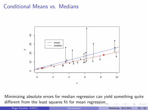
Conditional Means vs. Medians
●
●
●
●
●
●
●
●
●
●
●
●
●●
●
●
●
●
●
●
●
●
●
●
●
●
● ●
●
●
0 2 4 6 8 10
010
2030
40
x
y
●
●
meanmedian
Minimizing absolute errors for median regression can yield something quitedifferent from the least squares fit for mean regression.
Roger Koenker (UIUC) Introduction Meielisalp: 28.6.2011 39 / 58
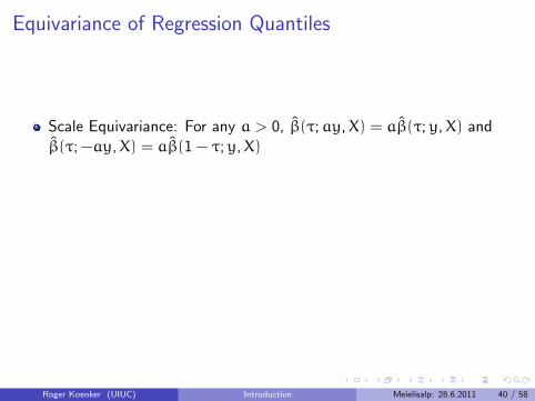
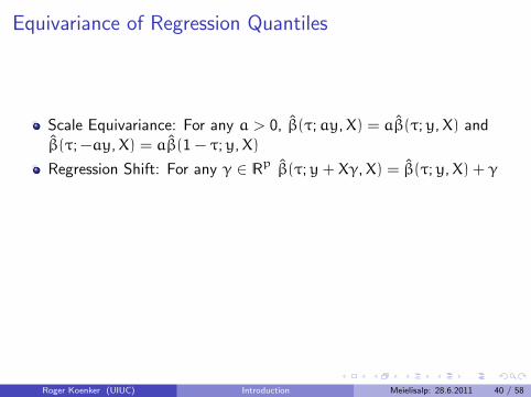
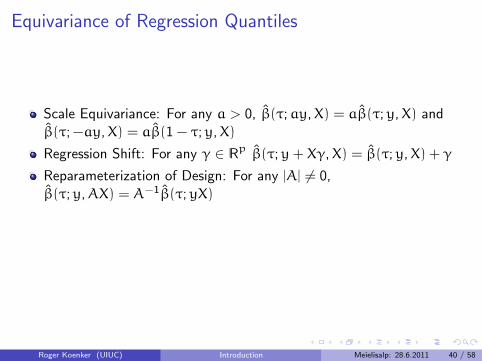
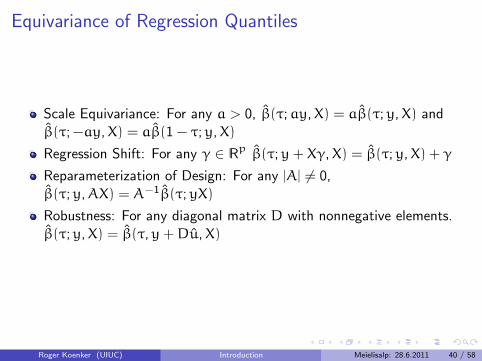
Equivariance of Regression Quantiles
Scale Equivariance: For any a > 0, β(τ;ay,X) = aβ(τ;y,X) andβ(τ; −ay,X) = aβ(1 − τ;y,X)
Regression Shift: For any γ ∈ |Rp β(τ;y+ Xγ,X) = β(τ;y,X) + γ
Reparameterization of Design: For any |A| 6= 0,β(τ;y,AX) = A−1β(τ;yX)
Robustness: For any diagonal matrix D with nonnegative elements.β(τ;y,X) = β(τ,y+Du,X)
Roger Koenker (UIUC) Introduction Meielisalp: 28.6.2011 40 / 58

Equivariance to Monotone Transformations
For any monotone function h, conditional quantile functions QY(τ|x) areequivariant in the sense that
Qh(Y)|X(τ|x) = h(QY|X(τ|x))
In contrast to conditional mean functions for which, generally,
E(h(Y)|X) 6= h(EY|X)
Examples:h(y) = min{0,y}, Powell’s (1985) censored regression estimator.h(y) = sgn{y} Rosenblatt’s (1957) perceptron, Manski’s (1975) maximumscore estimator. estimator.
Roger Koenker (UIUC) Introduction Meielisalp: 28.6.2011 41 / 58
Beyond Average Treatment Effects
Lehmann (1974) proposed the following general model of treatmentresponse:
“Suppose the treatment adds the amount ∆(x) when theresponse of the untreated subject would be x. Then thedistribution G of the treatment responses is that of the randomvariable X+ ∆(X) where X is distributed according to F.”
Roger Koenker (UIUC) Introduction Meielisalp: 28.6.2011 42 / 58
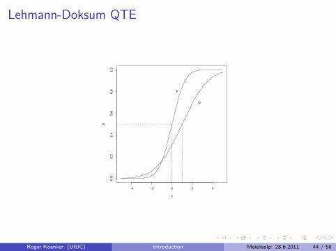
Lehmann QTE as a QQ-Plot
Doksum (1974) defines ∆(x) as the “horizontal distance” between F andG at x, i.e.
F(x) = G(x+ ∆(x)).
Then ∆(x) is uniquely defined as
∆(x) = G−1(F(x)) − x.
This is the essence of the conventional QQ-plot. Changing variables soτ = F(x) we have the quantile treatment effect (QTE):
δ(τ) = ∆(F−1(τ)) = G−1(τ) − F−1(τ).
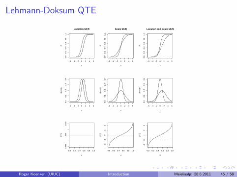
Roger Koenker (UIUC) Introduction Meielisalp: 28.6.2011 43 / 58
Lehmann-Doksum QTE
−4 −2 0 2 4
0.0
0.2
0.4
0.6
0.8
1.0
x
PG
F
Roger Koenker (UIUC) Introduction Meielisalp: 28.6.2011 44 / 58
Lehmann-Doksum QTE
−6 −4 −2 0 2 4 6
0.0
0.2
0.4
0.6
0.8
1.0
x
P
Location Shift
−6 −4 −2 0 2 4 6
0.0
0.1
0.2
0.3
0.4
x
dens
ity
0.0 0.2 0.4 0.6 0.8 1.0
0.99
01.
000
1.01
0
u
QT
E−6 −4 −2 0 2 4 6
0.0
0.2
0.4
0.6
0.8
1.0
x
P
Scale Shift
−6 −4 −2 0 2 4 60.
00.
10.
20.
30.
4
x
dens
ity
0.0 0.2 0.4 0.6 0.8 1.0
−2
−1
01
2
u
QT
E
−6 −4 −2 0 2 4 6
0.0
0.2
0.4
0.6
0.8
1.0
x
P
Location and Scale Shift
−6 −4 −2 0 2 4 6
0.0
0.1
0.2
0.3
0.4
x
dens
ity
0.0 0.2 0.4 0.6 0.8 1.0
−1
01
23
u
QT
E
Roger Koenker (UIUC) Introduction Meielisalp: 28.6.2011 45 / 58
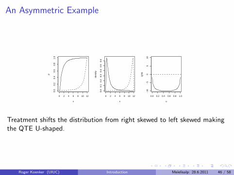
An Asymmetric Example
0 2 4 6 8 10 12
0.0
0.2
0.4
0.6
0.8
1.0
x
P
0 2 4 6 8 10 12
0.0
0.1
0.2
0.3
0.4
0.5
0.6
x
dens
ity0.0 0.2 0.4 0.6 0.8 1.0
−10
−5
05
10
u
QT
E
Treatment shifts the distribution from right skewed to left skewed makingthe QTE U-shaped.
Roger Koenker (UIUC) Introduction Meielisalp: 28.6.2011 46 / 58
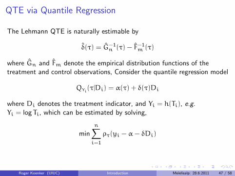
QTE via Quantile Regression
The Lehmann QTE is naturally estimable by
δ(τ) = G−1n (τ) − F−1
m (τ)
where Gn and Fm denote the empirical distribution functions of thetreatment and control observations, Consider the quantile regression model
QYi(τ|Di) = α(τ) + δ(τ)Di
where Di denotes the treatment indicator, and Yi = h(Ti), e.g.Yi = log Ti, which can be estimated by solving,
minn∑i=1
ρτ(yi − α− δDi)
Roger Koenker (UIUC) Introduction Meielisalp: 28.6.2011 47 / 58
Engel’s Food Expenditure Data
1000 2000 3000 4000 5000
500
1000
1500
2000
Household Income
Foo
d E
xpen
ditu
re
●
●
●
●
●
●●
●
●●
●
●
●
●
●
●
●
●
●
●
●
●
●
●
●
●
●
●
●●
●
●
●
●
●
●●
●
●●
●
●
●
●●
●
●
●
●●
●
●
●
●
●
●
●
●
●
●
●
●
●
●
●
●
●
●
●
●
●●
●
●
●
● ●●
●
●
●
●
●
●
●
●●
●
●
●
●●
●
●
●
●
●
●
●
●
● ●
●
●
●●
●
●
●
●
●
●
●●
●●
●
●
●
●
●
●
●
●
●
●●
●
●
●
●
●
●●
●
●
●
●
●
●
●
●
●
●
●●
●
●
●
●
●
●
●
●
●
●
●
●
●
●●●
●
●
●
●
●
●
●
●
●●●
●
●
●
●●
●
●
●
●
●
●
●
●●
●●
●
●
●●
●
●
●
●
● ●
●
●
●
●
●●
●
●●
●
●
●
●
●
●
●
●
●
●
●
●
●
●
●
●
●
●
●
●
●
●● ●
●
●
●
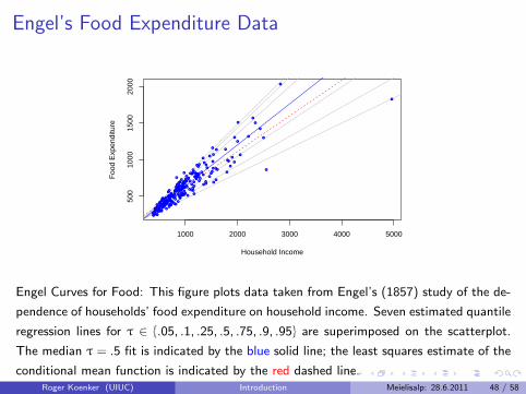
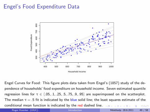
Engel Curves for Food: This figure plots data taken from Engel’s (1857) study of the de-
pendence of households’ food expenditure on household income. Seven estimated quantile
regression lines for τ ∈ {.05, .1, .25, .5, .75, .9, .95} are superimposed on the scatterplot.
The median τ = .5 fit is indicated by the blue solid line; the least squares estimate of the
conditional mean function is indicated by the red dashed line.Roger Koenker (UIUC) Introduction Meielisalp: 28.6.2011 48 / 58
Engel’s Food Expenditure Data
400 500 600 700 800 900 1000
300
400
500
600
700
800
Household Income
Foo
d E
xpen
ditu
re
●
●
●
●
●
●●
●
●
●
●
●
●
●
●
●
●
●
●
●
●
●
●
●
●
●
●
●
●
●
●
●
●
●
●
●
●
●
●
●
●
●
●
●
●
●
●
●
●
●
●
●
●●
●
●
●
●
●
●
●
●
●
●●
●
●
●
●
●
●
●
●
●●
●
●
●
●
●
●
●
●
●
●
●
●
●
●
●
●
●
●
●
●
●●
●●
●
●●●
●
●
●
●●
●
●
●
●
●
●
●
●
●
●
●
●
●
●
●
●
●
●
●
●
●
●●
●
●
●
●
●
●
●
●
●
●
●
●
●
●
●
●
●●
●
● ●●
●
●
Engel Curves for Food: This figure plots data taken from Engel’s (1857) study of the de-
pendence of households’ food expenditure on household income. Seven estimated quantile
regression lines for τ ∈ {.05, .1, .25, .5, .75, .9, .95} are superimposed on the scatterplot.
The median τ = .5 fit is indicated by the blue solid line; the least squares estimate of the
conditional mean function is indicated by the red dashed line.Roger Koenker (UIUC) Introduction Meielisalp: 28.6.2011 49 / 58
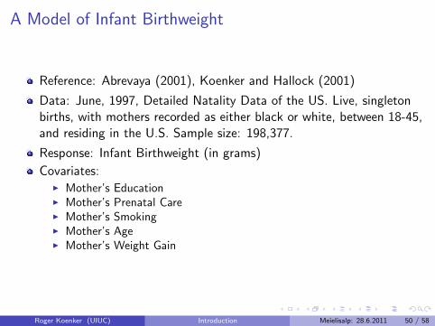
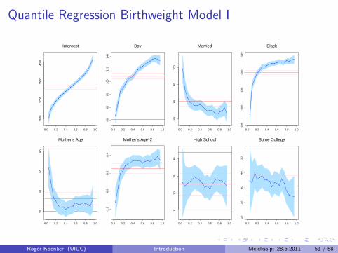
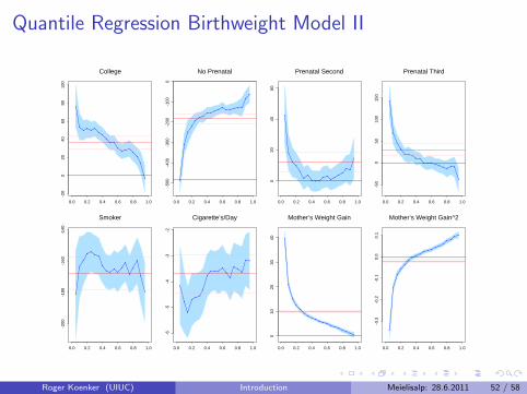
A Model of Infant Birthweight
Reference: Abrevaya (2001), Koenker and Hallock (2001)
Data: June, 1997, Detailed Natality Data of the US. Live, singletonbirths, with mothers recorded as either black or white, between 18-45,and residing in the U.S. Sample size: 198,377.
Response: Infant Birthweight (in grams)
Covariates:I Mother’s EducationI Mother’s Prenatal CareI Mother’s SmokingI Mother’s AgeI Mother’s Weight Gain
Roger Koenker (UIUC) Introduction Meielisalp: 28.6.2011 50 / 58
Quantile Regression Birthweight Model I
0.0 0.2 0.4 0.6 0.8 1.0
2500
3000
3500
4000
Intercept
•
•
•
•
••
••
••
••
••
••
•
•
•
0.0 0.2 0.4 0.6 0.8 1.0
4060
8010
012
014
0
Boy
•
•
•
•
•
••
•
•
••
••
••
• • • •
0.0 0.2 0.4 0.6 0.8 1.0
4060
8010
0
Married
•
•
•
••
• • ••
•• • •
••
• •
•
•
0.0 0.2 0.4 0.6 0.8 1.0
-350
-300
-250
-200
-150
Black
•
•
•
•
•
• • •• • • • • • •
• •• •
0.0 0.2 0.4 0.6 0.8 1.0
3040
5060
Mother’s Age
•
•
•
•
•• •
•• •
•
•• •
•• •
•
•
0.0 0.2 0.4 0.6 0.8 1.0
-1.0
-0.8
-0.6
-0.4
Mother’s Age^2
•
•
•
•
•• •
• • • ••
• • •• •
•
•
0.0 0.2 0.4 0.6 0.8 1.0
010
2030
High School
•
•
••
••
••
•
••
•
•
••
• ••
•
0.0 0.2 0.4 0.6 0.8 1.0
1020
3040
50
Some College
••
•
••
•
• ••
•
• ••
•
•
•
• • •
Roger Koenker (UIUC) Introduction Meielisalp: 28.6.2011 51 / 58
Quantile Regression Birthweight Model II
0.0 0.2 0.4 0.6 0.8 1.0
-20
020
4060
8010
0
College
•
•• • • •
••
•• •
•• • •
••
•
•
0.0 0.2 0.4 0.6 0.8 1.0
-500
-400
-300
-200
-100
0
No Prenatal
•
•
•
•
•• •
• •• •
•• • • • •
••
0.0 0.2 0.4 0.6 0.8 1.0
020
4060
Prenatal Second
•
•
••
•
••
• • •• •
••
••
• •
•
0.0 0.2 0.4 0.6 0.8 1.0
-50
050
100
150
Prenatal Third
•
•
•
•
• • •• •
• • •• • •
•• •
•
0.0 0.2 0.4 0.6 0.8 1.0
-200
-180
-160
-140
Smoker
•
•
•
• •• •
•
• ••
•
•
•
•
•
•
•
•
0.0 0.2 0.4 0.6 0.8 1.0
-6-5
-4-3
-2
Cigarette’s/Day
•
•
•
•• •
•
•
• • ••
•
•
••
•
• •
0.0 0.2 0.4 0.6 0.8 1.0
010
2030
40
Mother’s Weight Gain
•
•
•
•
••
•• •
• • •• • •
• • • •
0.0 0.2 0.4 0.6 0.8 1.0
-0.3
-0.2
-0.1
0.0
0.1
Mother’s Weight Gain^2
•
•
•
•
••
•• •
• • •• •
•• •
• •
Roger Koenker (UIUC) Introduction Meielisalp: 28.6.2011 52 / 58
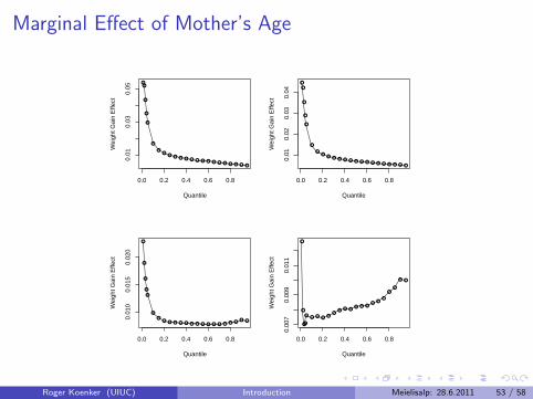
Marginal Effect of Mother’s Age
●●
●
●
●
●
●●
● ● ● ● ● ● ● ● ● ● ● ● ● ● ●
0.0 0.2 0.4 0.6 0.8
0.01
0.03
0.05
Quantile
Wei
ght G
ain
Effe
ct
●
●
●
●
●
●
●●
● ● ● ● ● ● ● ● ● ● ● ● ● ● ●
0.0 0.2 0.4 0.6 0.8
0.01
0.02
0.03
0.04
Quantile
Wei
ght G
ain
Effe
ct
●
●
●
●
●
●
●● ● ● ● ● ● ● ● ● ● ● ● ● ● ● ●
0.0 0.2 0.4 0.6 0.8
0.01
00.
015
0.02
0
Quantile
Wei
ght G
ain
Effe
ct
●
●
●●
● ● ● ● ●●
● ● ●● ● ●
● ●●
●●
● ●
0.0 0.2 0.4 0.6 0.8
0.00
70.
009
0.01
1
Quantile
Wei
ght G
ain
Effe
ct
Roger Koenker (UIUC) Introduction Meielisalp: 28.6.2011 53 / 58
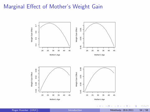
Marginal Effect of Mother’s Weight Gain
20 25 30 35 40 45
0.4
0.5
0.6
0.7
Mother's Age
Wei
ght G
ain
Effe
ct
20 25 30 35 40 45
0.45
0.55
0.65
Mother's Age
Wei
ght G
ain
Effe
ct
20 25 30 35 40 45
0.44
0.48
0.52
0.56
Mother's Age
Wei
ght G
ain
Effe
ct
20 25 30 35 40 45
0.45
0.50
0.55
0.60
Mother's Age
Wei
ght G
ain
Effe
ct
Roger Koenker (UIUC) Introduction Meielisalp: 28.6.2011 54 / 58
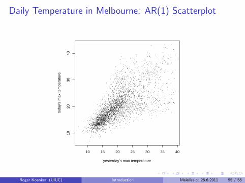
Daily Temperature in Melbourne: AR(1) Scatterplot
10 15 20 25 30 35 40
1020
3040
yesterday's max temperature
toda
y's
max
tem
pera
ture
Roger Koenker (UIUC) Introduction Meielisalp: 28.6.2011 55 / 58
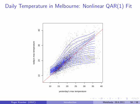
Daily Temperature in Melbourne: Nonlinear QAR(1) Fit
10 15 20 25 30 35 40
1020
3040
yesterday's max temperature
toda
y's
max
tem
pera
ture
Roger Koenker (UIUC) Introduction Meielisalp: 28.6.2011 56 / 58
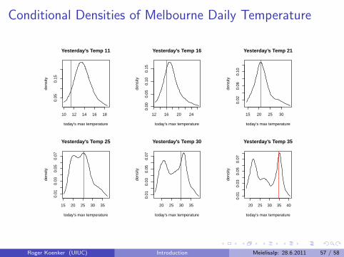
Conditional Densities of Melbourne Daily Temperature
10 12 14 16 18
0.05
0.15
today's max temperature
dens
ity
Yesterday's Temp 11
12 16 20 24
0.00
0.05
0.10
0.15
today's max temperature
dens
ity
Yesterday's Temp 16
15 20 25 30
0.02
0.06
0.10
today's max temperature
dens
ity
Yesterday's Temp 21
15 20 25 30 35
0.01
0.03
0.05
0.07
today's max temperature
dens
ity
Yesterday's Temp 25
20 25 30 35
0.01
0.03
0.05
0.07
today's max temperature
dens
ity
Yesterday's Temp 30
20 25 30 35 40
0.01
0.03
0.05
0.07
today's max temperature
dens
ity
Yesterday's Temp 35
Roger Koenker (UIUC) Introduction Meielisalp: 28.6.2011 57 / 58
Review
Least squares methods of estimating conditional mean functions
were developed for, and
promote the view that,
Response = Signal + iid (Gaussian Measurement Error
In fact the world is rarely this simple. Quantile regression is intended toexpand the regression window allowing us to see a wider vista.
Roger Koenker (UIUC) Introduction Meielisalp: 28.6.2011 58 / 58