Embed Size (px)
Citation preview
Portfolio Optimization & Monte Carlo Simulation
By
Magnus Erik Hvass Pedersen1
Hvass Laboratories Report HL-1401
First edition May 17, 2014
This revision August 3, 20142
Please ensure you have downloaded the latest revision of this paper from the internet:
www.hvass-labs.org/people/magnus/publications/pedersen2014portfolio-optimization.pdf
Source code and data files are also available from the internet:
www.hvass-labs.org/people/magnus/publications/pedersen2014portfolio-optimization.zip
Microsoft Excel spreadsheet with basic Kelly portfolio optimization is also available:
www.hvass-labs.org/people/magnus/publications/pedersen2014portfolio-optimization.xlsx
Abstract
This paper uses Monte Carlo simulation of a simple equity growth model with resampling of historical
financial data to estimate the probability distributions of the future equity, earnings and payouts of
companies. The simulated equity is then used with the historical P/Book distribution to estimate the
probability distributions of the future stock prices. This is done for Coca-Cola, Wal-Mart, McDonald’s and
the S&P 500 stock-market index. The return distributions are then used to construct optimal portfolios
using the “Markowitz” (mean-variance) and “Kelly” (geometric mean) methods. It is shown that variance is
an incorrect measure of investment risk so that mean-variance optimal portfolios do not minimize risk as
commonly believed. This criticism holds for return distributions in general. Kelly portfolios are correctly
optimized for investment risk and long-term gains, but the portfolios are often concentrated in few assets
and are therefore sensitive to estimation errors in the return distributions.
1 If you find any parts difficult to understand, or if you encounter any errors, whether logical, mathematical, spelling,
grammatical or otherwise, please mark the document and e-mail it to: Magnus (at) Hvass-Labs (dot) Org 2 See last page for revision history.

Portfolio Optimization & Monte Carlo Simulation
2
Nomenclature
IID Independent and identically distributed stochastic variables.
PDF Probability Density Function.
CDF Cumulative Distribution Function (Empirical).
Present value of future payouts, dividends and share-price.
Annual growth rate used in valuation.
Discount rate used in valuation.
k Kilo, a factor
m Million, a factor
b Billion, a factor
Infinity.
Price-to-Book ratio:
Number of shares outstanding.
Price per share.
Market capitalization (also written market-cap):
Capital supplied by shareholders as well as retained earnings, not per-share.
Earnings available for payout to shareholders, not per-share.
Dividend payout, pre-tax, not per-share.
Amount used for share buyback.
Amount of share issuance.
Share buyback net of issuance:
Net payout from company:
Part of earnings retained in company:
Return on Assets:
Return on Equity:
means that equals
means that is greater than or equal to
means that is approximately equal to
Implication: means that implies
Bi-implication: means that and
Multiplication: means that is multiplied by
Summation:
Multiplication:
Maximum of or . Similarly for
Logarithmic function with base (natural logarithm).
Absolute value of (the sign of is removed).
Probability of the stochastic variable being equal to .
Expected (or mean) value of the stochastic variable .
Variance of the stochastic variable .
Standard deviation of the stochastic variable :
Covariance of the stochastic variables and :

Portfolio Optimization & Monte Carlo Simulation
3
Introduction
Portfolio Optimization & Monte Carlo Simulation
4
1. Introduction There are two problems in constructing investment portfolios. First is to estimate the probability
distribution of possible returns on individual assets. Second is the combination of these assets into a
portfolio that optimally balances conflicting performance criteria.
A popular form of portfolio optimization is due to Markowitz [1] [2] which maximizes the portfolio’s mean
return and minimizes the variance. Such portfolios are called mean-variance optimal. The return variance is
commonly believed to measure investment risk so the mean-variance optimal portfolios are thought to
maximize the mean return while minimizing risk. However, the examples in sections 4.3 and 11.2 show that
variance is actually useless as a risk measure for investing.
For the future distribution of asset returns, Markowitz [2] vaguely proposed to use statistical analysis of
past asset returns adjusted with the probability beliefs of expert financial analysts. This paper takes another
approach by using Monte Carlo simulation of the equity growth model by Pedersen [3] which samples
historical financial data for a company and simulates its future equity, earnings, dividends, etc. and then
multiplies the simulated equity with samples of the historical P/Book distribution to estimate future stock
prices. This model is used on several companies as well as the S&P 500 stock-market index.
The Monte Carlo simulated stock returns are also used to construct so-called Kelly optimal portfolios [4],
which work as intended provided we know the true probability distributions of future asset returns. But
Kelly portfolios heavily weigh the assets with the best return distributions, so if the distributions are
incorrect then the Kelly portfolios may severely overweigh the wrong assets.
The paper also studies the complex historical relations between financial ratios such as P/Book and P/E for
the companies and S&P 500 index, and also compares them to the yield on USA government bonds.
1.1. Paper Overview The paper is structured as follows:
Section 2 describes the financial valuation formulas and the equity growth model.
Section 3 describes algorithms for Monte Carlo simulation.
Section 4 describes mean-variance portfolio optimization.
Section 5 describes Kelly portfolio optimization.
Section 6 briefly studies USA government bond yields.
Section 7 studies the S&P 500 stock-market index.
Sections 8, 9 and 10 study the companies Wal-Mart, Coca-Cola and McDonald’s.
Section 11 studies the mean-variance and Kelly optimal portfolios of these companies.
Section 12 is the conclusion.
Portfolio Optimization & Monte Carlo Simulation
5
1.2. Source Code & Data The experiments in this paper have been implemented in the statistical programming language R which is
freely available from the internet. The source-code and data-files are available at:
www.hvass-labs.org/people/magnus/publications/pedersen2014portfolio-optimization.zip
Time Usage
Executing this implementation on a consumer-level computer from the year 2011 typically requires only
seconds or minutes for an experiment consisting of a thousand Monte Carlo simulations. Implementing a
parallelized version or using another programming language might significantly decrease the time usage.

Portfolio Optimization & Monte Carlo Simulation
6
Theory
Portfolio Optimization & Monte Carlo Simulation
7
2. Present Value The present value of the dividend for future year is the amount that would have to be invested today with
an annual rate of return , also called the discount rate, so as to compound into becoming after
years:
Eq. 2-1
In Williams’ theory of investment value [5], the value of a company to its eternal shareholders is defined as
the present value of all future dividends. Let denote the present value of all future dividends prior to
dividend tax and not per share. Assume the discount rate is constant forever. If the company has no
excess cash, then the company will first have to generate earnings before paying dividends, so the present
value is calculated starting from the next year . The present value is then:
Eq. 2-2
2.1. Payout Instead of paying dividends, companies may also buy back or issue shares. Share buyback net of issuance is:
Eq. 2-3
The sum of dividends and net share buybacks is called payout:
Eq. 2-4
The term payout is a misnomer for share buybacks net of issuance as argued by Pedersen [6] [7], because a
share buyback merely reduces the number of shares outstanding which may have unexpected effects on
the share-price and hence does not constitute an actual payout from the company to its remaining
shareholders. A more accurate term for the combination of dividends and share buybacks would therefore
be desirable but the term payout will be used here and the reader should keep this distinction in mind.
The part of the earnings being retained in the company is:
Eq. 2-5
This is equivalent to:
Eq. 2-6
Portfolio Optimization & Monte Carlo Simulation
8
The ratio of earnings being retained in the company is:
Eq. 2-7
2.2. Equity Growth Model The company’s equity is the capital supplied directly by shareholders and the accumulation of retained
earnings. Earnings are retained for the purpose of investing in new assets that can increase future earnings.
Let be the equity at the end of year and let be the part of the earnings that are retained
in year . The equity at the end of year is then:
Eq. 2-8
The accumulation of equity is:
Eq. 2-9
The Return on Equity (ROE) is defined as a year’s earnings divided by the equity at the end of the previous
year. For year this is:
Eq. 2-10
This is equivalent to:
Eq. 2-11
Using this with the definition of payout from Eq. 2-6 gives:
Eq. 2-12
Portfolio Optimization & Monte Carlo Simulation
9
The present value to eternal shareholders is then:
Eq. 2-13
2.2.1. Normalized Equity
The accumulation of equity in Eq. 2-9 can be normalized by setting so it is independent of the
starting equity. This also normalizes the earnings calculated in Eq. 2-11 and the payouts calculated in Eq.
2-12, which allows for Monte Carlo simulation based solely on the probability distributions for and
so the results can easily be used with different starting equity.
2.3. Market Capitalization Let be the number of shares outstanding and let be the market-price per share. The
market-cap (or market capitalization, or market value) is the total price for all shares outstanding:
Eq. 2-14
The market-cap is frequently considered relative to the equity, which is also known as the price-to-book-
value or P/Book ratio:
Eq. 2-15
This is equivalent to:
Eq. 2-16
Because the starting equity is normalized to one in these Monte Carlo simulations, see section 2.2.1, it is
often convenient to express the formulas involving the market-cap in terms of the P/Book ratio instead.
2.4. Share Issuance & Buyback Share issuance and buyback changes the number of shares outstanding and hence affects the per-share
numbers, such as earnings per share, equity per share and price per share.
The number of shares is normalized by setting . If the share buyback and issuance occurs
when the shares are priced at then the number of shares changes according to the following
formula, see Pedersen [6] [7] for details:
Eq. 2-17
Portfolio Optimization & Monte Carlo Simulation
10
Where is defined in Eq. 2-3 and is calculated using Eq. 2-16 with Monte Carlo
simulated equity and P/Book ratio:
Eq. 2-18
The number of shares is then used with the Monte Carlo simulated equity, earnings, etc. to find the per-
share numbers. For example, the equity per share in year is calculated as:
Eq. 2-19
The price per share in year is calculated from Eq. 2-18 and Eq. 2-17:
Eq. 2-20
2.5. Value Yield The value yield is defined as the discount rate which makes the market-cap equal to the present value:3
Eq. 2-21
This may be easier to understand if the notation makes clear that the present value is a function of the
discount rate by writing the present value as . The value yield is then the choice of discount rate that
causes the present value to equal the market-cap:
Eq. 2-22
2.5.1. No Share Buyback & Issuance
First assume the company’s payout consists entirely of dividends so there are no share buybacks and
issuances and the number of shares remains constant.
The value yield for an eternal shareholder must then satisfy the equation:
Eq. 2-23
3 The value yield is also called the Internal Rate of Return (IRR) but that may be confused with the concept of the
Return on Equity (ROE) and is therefore not used here.
Portfolio Optimization & Monte Carlo Simulation
11
For a shareholder who owns the shares and receives dividends for years after which the shares are sold
at a price of , the value yield must satisfy the equation:
Eq. 2-24
2.5.2. Share Buyback & Issuance
If the company makes share buybacks and/or issuances then the number of shares changes and the present
value is calculated from the dividend per share instead of the total annual payout. For an eternal
shareholder, the value yield must satisfy:
Eq. 2-25
For a temporary shareholder who owns the shares and receives dividends for years after which the
shares are sold at a price of , the value yield must satisfy the equation:
Eq. 2-26
2.5.3. Tax
Taxes are ignored here but could also be taken into account. Let be the dividend tax-
rate and let be the capital gain tax-rate, both in year . Assuming there is a capital
gain when the shares are sold, the value yield must satisfy the equation:
Eq. 2-27
2.5.4. Interpretation as Rate of Return
The value yield is the annualized rate of return on an investment over its life or holding period, given the
current market price of that investment. This follows from the duality of the definition of the present value
from section 2, in which the present value may be considered as the discounting of a future dividend using
a discount rate , or equivalently the future dividend may be considered the result of exponential growth
of the present value using as the growth rate. The choice of that makes the present value equal to the
market-cap is called the value yield. This interpretation also extends to multiple future dividends that
spread over a number of years or perhaps continuing for eternity, where the present value is merely the
sum of all those future dividends discounted at the same rate.
Portfolio Optimization & Monte Carlo Simulation
12
Note that the value yield is not the rate of return on reinvestment of future dividends, which will depend
on the market price of the financial security at the time of such future dividends.
2.6. Terminal Value The present value of the equity growth model in Eq. 2-13 is defined from an infinite number of iterations,
but the Monte Carlo simulation must terminate after a finite number of iterations. Estimating the present
value is therefore done by separating into which is the present value of the payout in the
years that have been Monte Carlo simulated, and which is an approximation to the remaining
value if the Monte Carlo simulation had been allowed to continue for an infinite number of iterations:
Eq. 2-28
2.6.1. Mean Terminal Value
The mean terminal value can be estimated from the mean payout in year and the mean growth-rate
which is assumed to continue indefinitely. A lower bound for this mean terminal value is derived in [3]:
Eq. 2-29
For the equity growth model in section 2.2, the mean growth rate is:
Eq. 2-30
When the equity at the end of year is known, the mean payout can be calculated from Eq. 2-12:
Eq. 2-31
The number of Monte Carlo iterations must be chosen large enough so the distortion introduced by the
terminal value approximation is negligible. The formula for finding this number is given in [3].
Portfolio Optimization & Monte Carlo Simulation
13
3. Monte Carlo Simulation Monte Carlo simulation is computer simulation of a stochastic model repeated numerous times so as to
estimate the probability distribution of the outcome of the stochastic model. This is useful when the
probability distribution is not possible to derive analytically, either because it is too complex or because the
stochastic variables of the model are not from simple, well-behaved probability distributions. Monte Carlo
simulation allows for arbitrary probability distributions so that very rare events can also be modelled.
3.1. Equity Growth Model A single Monte Carlo simulation of the equity growth model consists of these steps:
1. Load historical financial data.
2. Determine the required number of Monte Carlo iterations using a formula from [3]. We set .
3. Set for normalization purposes.
4. For to : Sample , and from historical
data. The sampling is synchronized between companies as described below. Then calculate
from Eq. 2-11, from Eq. 2-12, from Eq. 2-8,
, and .
5. Calculate the mean terminal value using Eq. 2-29. For finite holding periods use the market-cap (or
share-price) as terminal value instead.
6. Use a numerical optimization method to find the value yield in Eq. 2-22.
The probability distribution is found by repeating steps 3-6 and recording the resulting value yields.
3.2. Market-Cap The simulated equity can be multiplied with a sample of the historical P/Book distribution to calculate the
market-cap, see Eq. 2-16. However, this ignores the strong correlation of successive P/Book ratios in the
historical data and may significantly distort the market-cap estimates, especially in the near future.
3.3. Per Share Calculating per-share numbers for equity, earnings, etc. consists of four steps:
1. The equity, earnings, share buyback net of issuance, etc. are simulated as described in section 3.1.
2. The market-cap is simulated as described in section 3.2.
3. The results of steps 1 and 2 are used with Eq. 2-17 and Eq. 2-18 to calculate the number of shares
after share buyback and issuance.
4. The equity, earnings, etc. from step 1 are divided by the number of shares from step 3 to find the
per-share numbers.
3.4. Synchronized Data Sampling The Monte Carlo simulation is performed for several companies simultaneously. To model any statistical
dependency that might be in the historical data, the data sampling is synchronized between the companies.
For example, the first year in the Monte Carlo simulation might use financial data from year 1998, the
second year in the simulation might use data from year 2005, the third year might use data from year 1994,
etc. This sequence of years is then used for all companies when sampling their historical financial data in
step 4 of the Monte Carlo algorithm in section 3.1.
Portfolio Optimization & Monte Carlo Simulation
14
Similarly, when historical P/Book ratios are sampled for calculating the market-cap and share-price, the
P/Book ratios are sampled from the same date for all companies. This is again done in an effort to model
any statistical dependencies in the historical data.
3.5. Warning This paper uses a simple financial model with resampling of historical financial data to simulate the future
finances and share-prices of companies, whose probability distributions are then used to construct
portfolios. This is a paradigm shift from merely using past share-prices when constructing portfolios.
However, the financial model is basic and has several limitations which should be kept in mind when
interpreting the results: The equity growth model may not be suitable for the companies considered here.
Growth decline should be modelled because the companies may otherwise outgrow the combined size of
all the companies in the S&P 500 index, which is unrealistic. The financial data may be insufficient and data
for more years might be needed e.g. to include long-term cycles. Older financial data should perhaps be
sampled less frequently than newer data. Calculating future share-prices from the simulated equity
multiplied with a sample of historical P/Book is a crude pricing model as mentioned in section 3.2.
Portfolio Optimization & Monte Carlo Simulation
15
4. Mean-Variance Portfolio Optimization Mean-variance portfolio optimization is originally due to Markowitz [1] [2]. A good description which also
covers more recent additions to the theory is given by Luenberger [8].
4.1. Portfolio Mean and Variance Let denote the rate of return for asset and let denote the asset’s weight in the
portfolio. For so-called long-only portfolios the assets can only be bought by the investor so the weights
must all be positive . For so-called long-and-short portfolios the assets can be bought or sold-
short so the weights can be either positive or negative. In both cases the weights must sum to one:
Eq. 4-1
The rate of return for the portfolio is:
Eq. 4-2
If there is uncertainty about the rate of return of an asset then is a stochastic variable which
means the portfolio’s rate of return is also a stochastic variable. The mean is an estimate of the rate of
return that can be expected from the portfolio. From the properties of the mean it follows that the
portfolio’s mean rate of return is defined directly from the asset mean rates of return:
Eq. 4-3
The actual return of the portfolio may be very different from its mean return. There are several ways of
measuring the degree of this uncertainty by measuring the spread of possible returns around the mean
portfolio return. A common measure of spread is the variance. From the properties of the variance it
follows that the portfolio’s variance is defined from the asset weights and the covariance of asset returns:
Eq. 4-4
The covariance measures how much the asset returns change together. A positive covariance means that
the two asset returns have a tendency to increase together and vice versa for a negative covariance. If the
covariance is zero then there is no consistent tendency for the asset returns to increase or decrease
together; but this does not mean that the asset returns are independent of each other, merely that their
relationship cannot be measured by the covariance.
The standard deviation of the portfolio’s rate of return is the square root of the variance.
Portfolio Optimization & Monte Carlo Simulation
16
4.2. Optimal Portfolios – The Efficient Frontier The mean and standard deviation of the asset returns can be plotted as in Figure 74. All possible portfolios
that can be obtained by altering the weights are contained in the so-called feasible set. The feasible set is
bordered by the so-called efficient frontier (also called the Pareto front in optimization terminology) which
minimizes the portfolio variance for every portfolio mean in the feasible set. The efficient frontier contains
the portfolios that are optimal in the sense that no lower variance can be obtained for a mean return. If we
know the mean asset returns and the covariance matrix, then the efficient frontier can be found using the
methods in [8].
4.3. Variance is Not Risk Mean-variance portfolios are commonly believed to minimize risk for a given level of expected return,
because variance is believed to measure risk. But this is an incorrect notion as proven with a short example.
Let asset A be a stochastic variable with negative returns (4%), (5%) or (6%) and let asset B be a stochastic
variable with positive returns 5%, 10% or 15%. The returns have equal probability of occurring and are
dependent in the order they are listed so that if asset A has return (4%) then asset B has return 5%, etc. The
asset returns are perfectly anti-correlated with coefficient -1.
The long-only, minimum-variance portfolio lies on the efficient frontier and is when the weight for asset A
is 5/6 and the weight for asset B is 1/6. This gives a portfolio with mean (2.5%) and zero variance, that is, all
possible returns of the portfolio are losses of exactly (2.5%). But an investor could instead have chosen a
portfolio consisting entirely of asset B which would always give a positive return of either 5%, 10% or 15%.
An investment entirely in asset B is clearly superior to an investment in the minimum-variance portfolio.
The above example had an asset with negative returns which could be avoided by adding the constraint
that returns must be positive; but the problem also exists for assets with partly negative returns or all
positive returns. To see this, change asset A’s possible returns to 3%, 2% or 1%. Then the minimum variance
portfolio still has asset A weight 5/6 and asset B weight 1/6 which gives a portfolio return of about 3.3%
with zero variance. But asset B alone would give a higher return of either 5%, 10% or 15%. So although the
minimum-variance portfolio has no return spread, it has a lower return with certainty.
The problem also exists for assets that have overlapping return distributions. Let asset A’s possible returns
be 6%, 5% or 4%. Then the minimum variance portfolio still has asset A weight 5/6 and asset B weight 1/6
which always gives a portfolio return of about 5.8% with zero variance. But asset B alone would give a
higher return of either 10% or 15% with probability 2/3 (or about 67%) and a slightly lower return of 5%
with probability 1/3 (or about 33%).
The reason asset A is included in the efficient frontier and minimum-variance portfolio is that its return has
a low (sample) standard deviation of 1% while asset B has a higher standard deviation of 5%. The two
assets have negative correlation so combining them in a portfolio lowers the combined standard deviation.
The mean-variance efficient frontier is optimized for low variance (and standard deviation) which gives a
low spread of the possible returns from the portfolio. But the spread of possible returns is not a useful
measure of risk because it does not consider the probability of loss and the probability of other assets
having a higher return. So the mean-variance portfolio is not optimized for risk in the traditional sense of
the word which is defined in a dictionary as “the chance of injury or loss”.

Portfolio Optimization & Monte Carlo Simulation
17
This is also demonstrated in section 11.2 with more complicated return distributions.
4.4. Value Yield The value yield is the annualized rate of return over several years or for eternity. The value yield can be
used as the rate of return in mean-variance portfolio optimization without changing the framework. The
above criticism still applies, namely that variance does not measure investment risk.
Portfolio Optimization & Monte Carlo Simulation
18
5. Kelly Portfolio Optimization Kelly [4] proposed a formula for determining how much of one’s capital to place on a bet given the
probability of gain and loss. The idea is to maximize the mean logarithmic growth-rate so that a sequence
of bets in the “long run” and on average will most likely outperform any other betting scheme, but in the
“short run” the Kelly betting may significantly underperform other betting schemes. The good and bad
properties of Kelly betting are summarized by MacLean et al. [9]. The Kelly criterion is used here for a
portfolio of assets where the returns of each asset are Monte Carlo simulated as described above.
5.1. One Asset Consider first the case where a single asset is available for investment. Let denote the
stochastic rate of return on the asset and let denote the fraction of the portfolio invested
in the asset. The remainder of the portfolio is held in cash which earns zero return.
The Kelly value (or Kelly criterion) is a function defined as:
Eq. 5-1
The objective is to find the asset weight that maximizes this Kelly value.
5.1.1. Only Positive Returns
If all asset returns are positive then the Kelly value in Eq. 5-1 increases as the asset weight increases. So the
Kelly value is unbounded and suggests that an infinite amount of one’s capital should be invested in the
asset using an infinite amount of leverage. This is because the cost of leverage is not taken into account.
5.2. Two Assets Now consider the case where two assets are available for investment whose returns are stochastic
variables denoted and . The portfolio is divided between these two assets.
The portfolio’s rate of return is the weighted sum of the asset returns:
Eq. 5-2
The Kelly value of the portfolio is:
Eq. 5-3
The objective is again to find the weight that maximizes the Kelly value.
5.2.1. One Asset and Government Bond
If one of the assets is a government bond then Eq. 5-3 has the bond yield as one of the asset returns:
Eq. 5-4
Portfolio Optimization & Monte Carlo Simulation
19
5.3. Multiple Assets Now consider a portfolio of multiple assets. Let denote the stochastic rate of return on
asset and let denote the weight of that asset in the portfolio. The portfolio’s rate of return is:
Eq. 5-5
The Kelly value is:
Eq. 5-6
The objective is again to find the weights that maximize the Kelly value.
5.3.1. Multiple Assets and Government Bond
If the portfolio can also contain a government bond then the portfolio’s rate of return is:
Eq. 5-7
The Kelly value is:
Eq. 5-8
The objective is again to find the weights that maximize the Kelly value.
5.4. Constraints on Asset Weights If the portfolio is so-called long-only then the weights must all be non-negative. If short-selling is allowed
then the weights can also be negative. If leverage (investing for borrowed money) is disallowed then the
sum of the weights must equal one. If leverage is allowed then the sum of the weights can exceed one.
5.5. Value Yield Recall from section 2.5.4 that the value yield is the annualized rate of return of an investment for a given
holding period or eternity. This means the value yield can be used as the asset return in the Kelly formulas
above. As demonstrated in the case studies below, the probability distribution for the value yield depends
on the holding period. For long holding periods the value yield is mostly affected by the dividend payouts
which are typically more stable, and for short holding periods the value yield is mostly affected by the
Portfolio Optimization & Monte Carlo Simulation
20
selling share-price which is more volatile. When using the value yield distributions in portfolio optimization
it is therefore assumed that the holding period matches that of the value yield distributions.
For example, if a portfolio is to be optimized for a 10-year holding period, then the value yield distributions
for 10-year holding periods should be used. Furthermore, if the portfolio may contain government bonds
then the current yield on bonds with 10-year maturity should be used. The government bond is assumed to
have a fixed yield if held until maturity, but if it is sold prior to its maturity then the selling price may cause
the annualized yield to differ significantly.
5.6. Optimization Method When the asset returns are Monte Carlo simulated, the probability distributions are discrete with equal
probability of all outcomes. An analytical method for determining the portfolio weights that maximize the
Kelly value does not seem to exist in the literature. The so-called L-BFGS-B method was tested for
numerically optimizing the Kelly value but it did not work. A heuristic optimizer is therefore used here.
5.6.1. Differential Evolution
Differential Evolution (DE) was proposed by Storn and Price [10] for optimization without the use of
gradients. DE works by having a population of candidate solutions for the optimization problem, which are
combined through several iterations in an effort to improve their performance on the optimization
problem. This process resembles evolution as it occurs in nature. DE is not guaranteed to converge to the
optimal solution but has been found to work in practice for many difficult optimization problems.
When optimizing Kelly portfolios, the candidate solutions of DE are different choices of portfolio weights
and the performance measure that is sought maximized is the Kelly value in Eq. 5-8.
Control Parameters
DE has several control parameters that affect its performance and ability to find the optimum. The
parameters used here are from Pedersen [11]. It may be necessary to select other parameters if the
number of assets is greatly increased.
Constraints
The DE implementation used here has a simple constraint handling system which has boundaries for the
portfolio weights, e.g. the weights must be between zero and one to disallow short-selling and leverage.
But the weights must also sum to one and this is enforced by dividing each weight with the sum of weights
in case the sum is greater than one. This works for simple constraints on the portfolio weights but if more
complicated constraints are needed then the constraint handling system must be extended.
5.7. Example of Correct Risk Minimization Recall from section 4.3 that mean-variance portfolio optimization did not minimize for investment risk. This
was demonstrated with two assets. Asset B is a stochastic variable with positive returns 5%, 10% or 15%.
Three cases for returns on asset A were considered. In the first case, asset A has negative returns (4%), (5%)
or (6%). In the second case, asset A has positive returns 3%, 2% or 1%. In the third case, asset A has positive
returns 6%, 5% and 4% which overlap with the returns of asset B. In all these cases the returns have equal
probability of occurring and are dependent in the order they are listed. Mean-variance portfolio
optimization failed to optimize all three cases because it would always include asset A in the minimum-
Portfolio Optimization & Monte Carlo Simulation
21
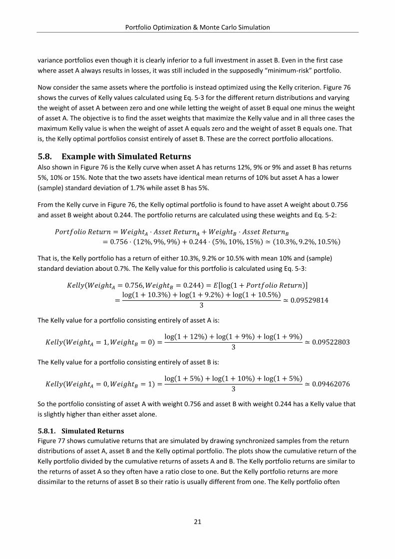
variance portfolios even though it is clearly inferior to a full investment in asset B. Even in the first case
where asset A always results in losses, it was still included in the supposedly “minimum-risk” portfolio.
Now consider the same assets where the portfolio is instead optimized using the Kelly criterion. Figure 76
shows the curves of Kelly values calculated using Eq. 5-3 for the different return distributions and varying
the weight of asset A between zero and one while letting the weight of asset B equal one minus the weight
of asset A. The objective is to find the asset weights that maximize the Kelly value and in all three cases the
maximum Kelly value is when the weight of asset A equals zero and the weight of asset B equals one. That
is, the Kelly optimal portfolios consist entirely of asset B. These are the correct portfolio allocations.
5.8. Example with Simulated Returns Also shown in Figure 76 is the Kelly curve when asset A has returns 12%, 9% or 9% and asset B has returns
5%, 10% or 15%. Note that the two assets have identical mean returns of 10% but asset A has a lower
(sample) standard deviation of 1.7% while asset B has 5%.
From the Kelly curve in Figure 76, the Kelly optimal portfolio is found to have asset A weight about 0.756
and asset B weight about 0.244. The portfolio returns are calculated using these weights and Eq. 5-2:
That is, the Kelly portfolio has a return of either 10.3%, 9.2% or 10.5% with mean 10% and (sample)
standard deviation about 0.7%. The Kelly value for this portfolio is calculated using Eq. 5-3:
The Kelly value for a portfolio consisting entirely of asset A is:
The Kelly value for a portfolio consisting entirely of asset B is:
So the portfolio consisting of asset A with weight 0.756 and asset B with weight 0.244 has a Kelly value that
is slightly higher than either asset alone.
5.8.1. Simulated Returns
Figure 77 shows cumulative returns that are simulated by drawing synchronized samples from the return
distributions of asset A, asset B and the Kelly optimal portfolio. The plots show the cumulative return of the
Kelly portfolio divided by the cumulative returns of assets A and B. The Kelly portfolio returns are similar to
the returns of asset A so they often have a ratio close to one. But the Kelly portfolio returns are more
dissimilar to the returns of asset B so their ratio is usually different from one. The Kelly portfolio often
Portfolio Optimization & Monte Carlo Simulation
22
grows exponentially more than asset B, but sometimes the Kelly portfolio decreases significantly relative to
asset B for extended periods.
The Kelly portfolio is optimal in the sense that in the “long run” its average growth is superior to all other
possible portfolios consisting of these two assets, but in the “short run” the Kelly portfolio can significantly
underperform, as evidenced in Figure 77.
5.9. Markowitz’ Opinion on the Kelly Criterion In Chapter VI of [2] Markowitz discussed the geometric mean return which is essentially the Kelly value in
Eq. 5-1, and concluded that: “The combination of expected return and variance which promises the greatest
return in the long run is not necessarily the combination which best meets the investor’s needs. The investor
may prefer to sacrifice long-run return for short-run stability.” But Markowitz does not seem to mention
that this alleged “stability” of mean-variance portfolios in fact may cause inferior returns and even losses,
as demonstrated in section 4.3.

Portfolio Optimization & Monte Carlo Simulation
23
Case Studies
Portfolio Optimization & Monte Carlo Simulation
24
6. USA Government Bonds Figure 1 shows the historical yield on USA government bonds for the periods 1798-2012 (averaged
annually) and 1962-2013 (averaged daily). During this period the bonds have had varying maturity period,
terms and taxation. Table 1 shows the statistics with a mean yield about 5% and standard deviation about
2%. Figure 2 shows the histograms of these historical bond yields and Figure 3 shows the cumulative
distribution functions. More statistics on USA government bonds are given by Pedersen [3].
7. S&P 500 The Standard & Poor’s 500 stock market index (S&P 500) consists of 500 large companies traded on the
stock markets in USA and operating in a wide variety of industries including energy and utility, financial
services, health care, information technology, heavy industry, manufacturers of consumer products, etc.
The S&P 500 index may be used as a proxy for the entire USA stock market as it covers about 75% of that
market.4
7.1. Financial Data Table 2 shows financial ratios for the S&P 500 and statistics are shown in Table 3. Figure 4 shows the
historical stock-price. The earnings yield is shown in Figure 5, the P/Book is shown in Figure 6, the P/E is
shown in Figure 7 and statistics are shown in Table 4. Figure 8 compares the P/Book and P/E which shows a
complex relation caused by the earnings having greater volatility than the book-value.
7.1.1. Comparison to USA Government Bonds
Figure 9 compares the yield on USA government bonds with 10-year maturity to the earnings yield and
P/Book of the S&P 500, which shows complex relations. Figure 10 shows the difference between the
earnings yield of the S&P 500 and the yield on USA government bonds which varies through time from
negative (3.6%) to positive 5.9% with negative mean (0.4%), see Table 5. So if the S&P 500 had paid out all
its earnings as dividends then the average rate of return would have been 0.4% (that is, percentage points)
lower than the rate of return that could be obtained from investing in USA government bonds. This means
the S&P 500 would either have to grow its earnings or the participants of the capital market viewed the
S&P 500 as having lower risk than USA government bonds. This so-called equity risk premium between the
S&P 500 and USA government bonds is studied in more detail by Pedersen [3]. The conclusion is that there
is no consistent and predictable relation between the yield on USA government bonds and the rate of
return on the S&P 500 stock-market index.
7.2. Value Yield The Monte Carlo simulation described in section 3 is performed 2,000 times using the financial ratios for
the S&P 500 stock-market index in Table 2. The starting P/Book ratio for the S&P 500 is set to 2.6 calculated
from the share-price of about USD 1,880 on April 24, 2014 divided by the last-known equity of USD 715.84
on December 31, 2013. The current P/Book of 2.6 is slightly below the historical average of 2.9, see Table 4.
4 S&P 500 Fact Sheet, retrieved April 11, 2013:
www.standardandpoors.com/indices/articles/en/us/?articleType=PDF&assetID=1221190434733
Portfolio Optimization & Monte Carlo Simulation
25
The Monte Carlo simulation provides estimates of future equity, earnings, dividends, etc. but only the value
yield is used here. Recall that the value yield is the annualized rate of return an investor would get from
making an investment and holding it for a number of years, see section 2.5.4.
Figure 11 shows the mean and standard deviation for the value yield for holding periods up to 30 years.
Note that the standard deviation decreases as the holding period increases. This is because when the
holding period is short, the value yield is greatly affected by the selling price which is more volatile. When
the holding period is long, the value yield is dominated by the dividend payouts which are more stable.
Figure 12 shows the value yield distribution for 10 year holding periods and Figure 13 shows them for
eternal holding periods. The value yield distributions with and without share buyback simulation are shown
and although the difference is small it is not zero. Unless otherwise noted in the following we will use the
value yield with share buyback simulation.
8. Wal-Mart The company Wal-Mart is an international retailer and was founded in 1962 in USA.
8.1. Financial Data Table 6 shows financial data for Wal-Mart. Financial ratios are shown in Table 7 and statistics are shown in
Table 8. Note the low standard deviation of all these ratios except the ones regarding the allocation of
earnings between dividends, share buyback and retaining.
Figure 14 shows the historical share-price. The earnings yield is shown in Figure 15, the P/Book is shown in
Figure 16, the P/E is shown in Figure 17 and statistics are shown in Table 9. Figure 18 compares the P/Book
and P/E which shows an almost linear relation caused by the stability of ROE so the earnings were closely
related to the book-value (equity) and hence P/E is closely related to P/Book, see Table 8.
8.1.1. Comparison to USA Government Bonds
Figure 19 compares the yield on USA government bonds to the earnings yield and P/Book of Wal-Mart
which shows complex relations that are somewhat correlated; the earnings yield has negative correlation
coefficient (0.61) and the P/Book has positive correlation coefficient 0.44.
Figure 20 shows the difference between the earnings yield of Wal-Mart and the yield on USA government
bonds. The statistics are shown in Table 11 and range between (4.9%) and 7.5% with mean 0.5%.
There is no clear and simple relation between the pricing of Wal-Mart shares and USA government bonds.
8.1.2. Comparison to S&P 500
Figure 21 compares the earnings yield, P/Book and P/E for Wal-Mart and the S&P 500 index. The relations
are complex but the P/Book is highly correlated with coefficient 0.85, see Table 10.
Figure 22 shows the difference between the earnings yield of Wal-Mart and the S&P 500 index. The
statistics are shown in Table 11. There is no consistent and predictable difference in earnings yield.
Portfolio Optimization & Monte Carlo Simulation
26
8.2. Value Yield The Monte Carlo simulation described in section 3 is performed 2,000 times using the financial ratios for
Wal-Mart in Table 7. The starting P/Book ratio for Wal-Mart is set to 3.3 calculated from the market-cap of
USD 253b on April 24, 2014 and divided by the last-known equity of USD 76b on January 31, 2014. The
current P/Book of 3.3 is considerably less than the historical average of 4.7, see Table 9, and historically the
P/Book has been greater than 3.3 about 70% of the time, see the P/Book CDF plot in Figure 16.
Figure 23 shows the mean and standard deviation for the value yield for holding periods up to 30 years. As
noted previously, the standard deviation decreases as the holding period increases. Figure 24 shows the
value yield distribution for 10 year holding periods and Figure 25 shows it for eternal holding periods.
8.2.1. Comparison to S&P 500
Figure 26 compares the value yields of Wal-Mart and the S&P 500 index for 10-year holding periods, which
has positive correlation with coefficient 0.77, see Table 24. Figure 27 compares the value yields for eternal
holding which has a positive but lower correlation with coefficient 0.34, see Table 25.
Figure 28 shows the value yield difference between Wal-Mart and the S&P 500 index for 10-year holding
periods. The value yield differences are almost all positive and are about 7.5% on average. This means
nearly all the value yields of Wal-Mart are greater than those of the S&P 500 index.
Figure 29 shows the distribution of value yield difference for eternal holding of Wal-Mart and the S&P 500
index. The value yield differences are almost all greater than 3.5% with mean about 5%. This means the
value yield of Wal-Mart is at least 3.5% (percentage points) greater than that of the S&P 500 index, and on
average the difference is 5% (percentage points).
The large differences in the value yields of these Monte Carlo simulations are partially caused by Wal-
Mart’s dividend per share growing 12% per year on average while the dividend of the S&P 500 index only
grows 6.3%. Furthermore, for 10-year holding periods the share-price significantly affects the value yield.
The S&P 500 is currently trading slightly below its historical average P/Book while Wal-Mart is currently
trading much below its historical average. As future share-prices are calculated here by sampling the
historical P/Book distribution, the share-prices of Wal-Mart are likely to increase more than those of the
S&P 500 index.
9. Coca-Cola The company Coca-Cola was incorporated in 1919 in USA but its origin is significantly older. The company
produces beverages that are sold worldwide.
9.1. Financial Data Table 12 shows financial data for Coca-Cola. Financial ratios are shown in Table 13 and statistics are shown
in Table 14. Note that all these ratios are considerably more volatile than those of Wal-Mart in Table 8.
Figure 30 shows the historical share-price. The earnings yield is shown in Figure 31, the P/Book is shown in
Figure 32, the P/E is shown in Figure 33 and statistics are shown in Table 15. Figure 34 compares the
P/Book and P/E which shows a complex relation but with a high correlation coefficient of 0.78.
Portfolio Optimization & Monte Carlo Simulation
27
9.1.1. Comparison to USA Government Bonds
Figure 35 compares the yield on USA government bonds to the earnings yield and P/Book of Coca-Cola
which shows complex relations but strong correlations; the earnings yield has negative correlation
coefficient (0.62) and the P/Book has positive correlation coefficient 0.72. This means that there has been a
historical tendency for the P/Book to increase with the yield of USA government bonds although in a
complex and unpredictable pattern.
Figure 36 shows the difference between the earnings yield of Coca-Cola and the yield on USA government
bonds. The statistics are shown in Table 17 and range between (5.3%) and 5.5% with mean (0.4%). There is
no consistent and predictable premium between the earnings yield of Coca-Cola and the yield on USA
government bonds.
9.1.2. Comparison to S&P 500
Figure 37 compares the earnings yield, P/Book and P/E for Coca-Cola and the S&P 500 index. The relations
are complex but the P/Book is somewhat correlated with coefficient 0.69, see Table 16.
Figure 38 shows the difference between the earnings yield of Coca-Cola and the S&P 500 index. The
statistics are shown in Table 17. There is no consistent and predictable difference in earnings yield.
9.2. Value Yield The Monte Carlo simulation described in section 3 is performed 2,000 times using the financial ratios for
Coca-Cola in Table 13. The starting P/Book ratio for Coca-Cola is set to 5.5 calculated from the market-cap
of USD 179b on April 24, 2014 and divided by the last-known equity of USD 33b on March 28, 2014. The
current P/Book of 5.5 is almost half of the historical average of 10.7, see Table 15, and historically the
P/Book has been greater than 5.5 more than 75% of the time, see the P/Book CDF plot in Figure 32.
Figure 39 shows the mean and standard deviation for the value yield for holding periods up to 30 years. As
noted previously, the standard deviation decreases as the holding period increases. Figure 40 shows the
value yield distribution for 10 year holding periods and Figure 41 shows it for eternal holding periods.
9.2.1. Comparison to S&P 500
Figure 42 compares the value yields of Coca-Cola and the S&P 500 index for 10-year holding periods, which
has positive correlation with coefficient 0.65, see Table 24. Figure 43 compares the value yields for eternal
holding which has a slightly positive correlation with coefficient 0.16, see Table 25.
Figure 44 shows the value yield difference between Coca-Cola and the S&P 500 index for 10-year holding
periods. The value yield differences are almost all positive and are about 12.5% on average. This means
nearly all the value yields of Coca-Cola are greater than those of the S&P 500 index.
Figure 45 shows the distribution of value yield difference for eternal holding of Coca-Cola and the S&P 500
index. The value yield differences are all greater than 5% with mean about 8%. This means the value yield
of Coca-Cola is at least 5% (percentage points) greater than that of the S&P 500 index, and on average the
difference is 8% (percentage points).
The large differences in the value yields of these Monte Carlo simulations are partially caused by Coca-
Cola’s dividend per share growing 13% per year on average while the dividend of the S&P 500 index only
Portfolio Optimization & Monte Carlo Simulation
28
grows 6.3%. Furthermore, for 10-year holding periods the share-price significantly affects the value yield.
The S&P 500 is currently trading slightly below its historical average P/Book while Coca-Cola is currently
trading at half its historical average. As future share-prices are calculated by sampling the historical P/Book
distribution, the share-prices of Coca-Cola are likely to increase more than those of the S&P 500 index.
10. McDonald’s The company McDonald’s was started by two brothers in USA in 1948 as a single restaurant selling fast-
food at low prices. The company now sells its fast-food worldwide.
10.1. Financial Data Table 18 shows financial data for McDonald’s. Financial ratios are shown in Table 19 and statistics are
shown in Table 20. Note that all these ratios are volatile with high standard deviation except for the ratio of
equity to assets.
Figure 46 shows the historical share-price. The earnings yield is shown in Figure 47, the P/Book is shown in
Figure 48, the P/E is shown in Figure 49 and statistics are shown in Table 21. Figure 50 compares the
P/Book and P/E which shows a complex relation with a somewhat low correlation coefficient of 0.25.
10.1.1. Comparison to USA Government Bonds
Figure 51 compares the yield on USA government bonds to the earnings yield and P/Book of McDonald’s
which shows complex relations. The earnings yield has negative correlation coefficient (0.14) and the
P/Book has negative correlation coefficient (0.53).
Figure 52 shows the difference between the earnings yield of McDonald’s and the yield on USA government
bonds. The statistics are shown in Table 23 and range between (3.3%) and 4.9% with mean 0.4%. There is
no consistent and predictable premium between the earnings yield of McDonald’s and the yield on USA
government bonds.
10.1.2. Comparison to S&P 500
Figure 53 compares the earnings yield, P/Book and P/E for McDonald’s and the S&P 500 index. The
relations are complex. The correlation coefficients are shown in Table 22 but are not useful in describing
these complex relations.
Figure 54 shows the difference between the earnings yield of McDonald’s and the S&P 500 index. The
statistics are shown in Table 23 and range between (1.7%) and 4.8% with mean 0.7%. There is no consistent
and predictable difference in earnings yield.
10.2. Value Yield The Monte Carlo simulation described in section 3 is performed 2,000 times using the financial ratios for
McDonald’s in Table 19. The starting P/Book ratio for McDonald’s is set to 6.2 calculated from the market-
cap of USD 99b on April 24, 2014 and divided by the last-known equity of USD 16b on December 31, 2013.
The current P/Book of 6.2 is much higher than the historical average of 4.0, see Table 21. Historically the
P/Book has been lower than 6.2 more than 90% of the time, see the P/Book CDF plot in Figure 48.
Portfolio Optimization & Monte Carlo Simulation
29
Figure 55 shows the mean and standard deviation for the value yield for holding periods up to 30 years. As
noted previously, the standard deviation decreases as the holding period increases.
10.2.1. Holding for 10 Years
Figure 56 shows the value yield distribution for 10 year holding periods. The value yield of McDonald’s for
10 year holding periods is negative with probability 0.13 (or 13%). The probability is 0.40 (or 40%) that the
value yield of McDonald’s is less than the yield on USA government bonds with 10 year maturity, which was
about 2.7% in late April 2014. On average the value yield of McDonald’s is 3.7%.
The high probability of loss is due to two things: (1) The current P/Book of McDonald’s is historically high
and future share-prices are Monte Carlo simulated with mostly lower P/Book, and (2) the historical ROE is
much lower than it has been in recent years so the simulated future earnings and the accumulation of
equity is lower than it has been in recent years. The combined effect is a Monte Carlo simulated share-price
that is often lower than it is today.
10.2.2. Holding for Eternity
Figure 57 shows the value yield distribution for eternal holding periods. When the effect of share buybacks
is also Monte Carlo simulated then the value yield ranges between 6.5-9.5%. This is a large increase from
the value yield for 10-year holding periods. The reason is that the volatile share-price has a small impact on
the value yield when the holding period is eternity as there is no selling share-price. It is the dividends that
determine the value yield. Furthermore, the decreasing share-price has a positive effect on the value yield
when share buybacks are simulated because shares are bought back in the future at relatively lower prices.
10.2.3. Comparison to S&P 500
Figure 58 compares the value yields of McDonald’s and the S&P 500 index for 10-year holding periods,
which has almost zero correlation, see Table 24. Figure 59 compares the value yields for eternal holding
which has a positive correlation with coefficient 0.56, see Table 25.
Figure 60 shows the value yield difference between McDonald’s and the S&P 500 index for 10-year holding
periods. The probability of McDonald’s value yield being less than that of the S&P 500 is 0.88 (or 88%). The
value yield difference ranges between (14%) and 4% with mean (5.9%).
Figure 61 shows the distribution of value yield difference for eternal holding of McDonald’s and the S&P
500 index. The probability of McDonald’s value yield being less than that of the S&P 500 is 0.97 (or 97%).
The value yield difference ranges between (2.1%) and 0.6% with mean (0.7%).
In both cases, nearly all the value yields of McDonald’s are less than those of the S&P 500. For the 10-year
holding period this is partially caused by the decrease in McDonald’s simulated share-price as described
above. For eternal holding the reason is that a high share-price is currently being paid for McDonald’s
shares with a P/Book of 6.2 and the Monte Carlo simulated dividend per share grows about 6.4% per year
on average. For the S&P 500 the dividend per share grows slightly less at about 6.3% per year on average,
but shares of the S&P 500 are much lower priced at a P/Book of only 2.6. The initial simulated dividend
yield is higher for the S&P 500 than for McDonald’s and because of the similar growth rates it is currently
cheaper to purchase the dividend stream of the S&P 500 index than McDonald’s. The result is that S&P 500
has a higher value yield than McDonald’s.
Portfolio Optimization & Monte Carlo Simulation
30
11. Portfolios This section optimizes portfolios of the companies that were studied individually in the previous sections.
11.1. Value Yield Comparison The previous sections compared the value yields of the companies to that of the S&P 500 stock-market
index. This section compares the value yields amongst companies. As described in section 3.4, the Monte
Carlo simulations of companies are synchronized so that historical financial data is sampled from the same
year amongst companies. This is done to account for statistical dependencies between the companies.
11.1.1. Wal-Mart & Coca-Cola
Figure 62 compares the value yields of Wal-Mart and Coca-Cola for 10-year holding periods which are
positively correlated with coefficient 0.47, see Table 24. Figure 63 compares the value yields for eternal
holding which are negatively correlated with coefficient (0.22), see Table 25.
Figure 64 shows the distribution of value yield differences between Wal-Mart and Coca-Cola for 10-year
holding periods where there is a probability of 0.88 (or 88%) that Wal-Mart has a lower value yield than
Coca-Cola, see Table 26. The value yield difference is on average about 5% (percentage points).
Figure 65 shows the value yield differences for eternal holding where there is a probability of 0.998 (or
99.8%) that Wal-Mart has a lower value yield than Coca-Cola, see Table 27. The value yield difference is on
average about 3% (percentage points).
11.1.2. McDonald’s & Coca-Cola
Figure 66 compares the value yields of McDonald’s and Coca-Cola for 10-year holding periods which are
slightly negatively correlated with coefficient (0.1), see Table 24. Figure 67 compares the value yields for
eternal holding which are nearly uncorrelated with coefficient 0.03, see Table 25.
Figure 68 shows the distribution of value yield differences between McDonald’s and Coca-Cola for 10-year
holding periods where there is a probability of almost 1 (or 100%) that McDonald’s has a lower value yield
than Coca-Cola, see Table 26. The value yield difference is on average about 18% (percentage points).
Figure 69 shows the value yield differences for eternal holding where there is a probability of 1 (or 100%)
that McDonald’s has a lower value yield than Coca-Cola, see Table 27. The value yield difference is on
average about 9% (percentage points).
11.1.3. McDonald’s & Wal-Mart
Figure 70 compares the value yields of McDonald’s and Wal-Mart for 10-year holding periods which are
slightly negatively correlated with coefficient (0.11), see Table 24. Figure 71 compares the value yields for
eternal holding which are slightly positively correlated with coefficient 0.19, see Table 25.
Figure 72 shows the distribution of value yield differences between McDonald’s and Wal-Mart for 10-year
holding periods where there is a probability of almost 1 (or 100%) that McDonald’s has a lower value yield
than Wal-Mart, see Table 26. The value yield difference is on average about 13% (percentage points).
Portfolio Optimization & Monte Carlo Simulation
31
Figure 73 shows the value yield differences for eternal holding where there is a probability of 1 (or 100%)
that McDonald’s has a lower value yield than Wal-Mart, see Table 27. The value yield difference is on
average almost 6% (percentage points).
11.1.4. Ordering
The value yields can be ordered as follows:
USA Government Bond < McDonald’s < S&P 500 < Wal-Mart < Coca-Cola
That is, the annualized rate of return on Coca-Cola is mostly greater than that of Wal-Mart, which is mostly
greater than that of the S&P 500, which is mostly greater than that of McDonald’s, which is mostly greater
than the yield on USA government bonds. However, the probabilities are not equal to one.
For 10-year holding periods there is a probability of 0.6 (or 60%) that the yield on USA government bonds is
less than the value yield of McDonald’s; and there is a probability of 0.88 (or 88%) that the value yield of
McDonald’s is less than that of the S&P 500; and there is a probability of 0.82 (or 82%) that the value yield
of Wal-Mart is less than that of Coca-Cola; see Table 26 and Table 28. The probabilities can be written
above the inequality signs in the ordering:
USA Government Bond <0.6 McDonald’s <0.88 S&P 500 <0.9965 Wal-Mart <0.82 Coca-Cola
Eq. 11-1
For eternal holding periods the relation is almost rigid as the probabilities are nearly one, see Table 27 and
Table 28. The ordering is:
USA Government Bond <1 McDonald’s <0.97 S&P 500 <1 Wal-Mart <0.998 Coca-Cola
Eq. 11-2
11.1.5. Correlation
The value yields are somewhat correlated as shown in the scatter-plots and summarized in Table 24 and
Table 25. However, the correlation coefficients change magnitude and in some cases also change signs for
the different holding periods considered here. For example, for 10-year holding periods the value yields of
Wal-Mart and Coca-Cola are positively correlated with coefficient 0.47 but for eternal holding the value
yields are negatively correlated with coefficient (0.22).
11.2. Mean-Variance Optimal Portfolios This section optimizes portfolios with regard to the mean and variance as described in section 4, using the
Monte Carlo simulated value yields described in the previous sections.
11.2.1. Holding for 10 Years
The mean-variance efficient portfolios for 10-year holding periods are shown in Figure 74 and the portfolio
weights are shown in Table 29 and Table 30. Note that McDonald’s is contained in most of the efficient
frontier for the long-only portfolios and is contained in the entire efficient frontier for the long-and-short
portfolios. This is in spite of McDonald’s having a probability of nearly 1 (or 100%) of having a lower value
yield than all the other assets available for the portfolio, see Table 26, and furthermore there is a
Portfolio Optimization & Monte Carlo Simulation
32
probability of 0.13 (or 13%) that McDonald’s value yield is less than zero and there is a probability of 0.4 (or
40%) that McDonald’s value yield is less than the return on USA government bonds, see Table 28.
11.2.2. Holding for Eternity
The mean-variance efficient frontiers for eternal holding periods are shown in Figure 75 and the portfolio
weights are shown in Table 31 and Table 32. Note that McDonald’s is contained in half of the efficient long-
only portfolios and almost all of the efficient long-and-short portfolios. This is in spite of McDonald’s having
probability almost one of having a lower rate of return than the other assets, see Table 27.
11.2.3. Variance is Not Risk
The efficient portfolios contain McDonald’s even though it is almost certain to have a lower value yield than
the other assets available for the portfolio. Furthermore, for 10-year holding periods there is a significant
risk of McDonald’s having a lower value yield than the yield on USA government bonds – as well as a
significant risk of McDonald’s value yield being negative.
The reason McDonald’s is included in the mean-variance efficient frontier is that McDonald’s value yields
have a low variance (and standard deviation). The mean-variance efficient frontier is optimized for low
variance which gives a low spread of the possible returns on the portfolio. But the spread of possible
returns is not a useful measure of investment risk because it does not consider the probability of loss and
the probability of other assets having a higher return. This criticism holds in general, see section 4.3.
11.3. Kelly Optimal Portfolios Recall the plots in Figure 74 showed the efficient frontier for mean-variance optimal portfolios, that is, the
curved line where portfolios have maximum mean and minimum variance. Because there were two
measures of performance – mean and variance – it was convenient to show the trade-off between these
two conflicting performance measures in a 2-dimensional plot.
This section optimizes portfolios with regard to the Kelly value as described in section 5.3.1, using the
Monte Carlo simulated value yields described in the previous sections. But for Kelly portfolios there is only
one performance measure: The Kelly value. So it is only necessary to find the portfolio that maximizes the
Kelly value and a plot is unnecessary. However, Kelly portfolios have a tendency to heavily weigh the best
assets and possibly let the entire portfolio consist of only one asset if it is likely that it will outperform all
other combinations of assets. This is demonstrated below.
11.3.1. Holding for 10 Years
In the following, the value yield that is sought optimized is the annualized rate of return for a 10-year
holding period of the assets in the portfolio. The portfolio may also include government bonds whose yield
for 10-year maturity was 2.7% in late April 2014.
Long Only
Table 33 shows the Kelly optimal portfolios when the asset weights must all be positive (that is, long-only).
When the asset weights are bounded to [0.0, 0.1], that is, when the minimum asset weight is zero and the
maximum asset weight is 0.1, then the Kelly optimal portfolio has weight 0.1 for all four assets and weight
0.6 for the government bond. The value yield mean is 6.8% with standard deviation 1.2%. There is a
probability of 0.42 (or 42%) that this portfolio has a lower value yield than the minimum-variance portfolio
whose weights are shown in Table 29.
Portfolio Optimization & Monte Carlo Simulation
33
As the asset weight limit is increased, the worse performing assets are gradually removed from the Kelly
portfolios. The government bond and McDonald’s are removed first, then the S&P 500 index, and finally
Wal-Mart is gradually removed until only Coca-Cola remains in the Kelly portfolio. This is consistent with
the discussion in section 11.1.4 regarding the order of attractiveness for these assets.
Also shown in Table 33 are the Kelly values and standard deviations of returns which both increase for
these Kelly portfolios, so the Kelly optimization disregards the spread of possible returns, which is what is
sought minimized in mean-variance portfolios. The probability is one of the Kelly portfolios outperforming
the minimum-variance (aka “minimum-risk”) portfolio, except for the first Kelly portfolio whose weights
were too constrained.
The minimum-variance portfolio in Table 29 has an almost 50/50 division between S&P 500 and
McDonald’s because they each have low variance and their combination gives even lower variance for the
portfolio. Conversely, the Kelly optimal portfolios weigh Wal-Mart and especially Coca-Cola heavily and
discard both S&P 500 and McDonald’s from the portfolio when the weight constraints allow it.
Note that the Kelly portfolios are allowed to contain a government bond which is assumed to have zero-
variance return. However, the government bond is only included in the Kelly portfolios with low asset
weight boundaries so the other asset weights are low and the government bond is included of necessity.
Long & Short
Table 34 shows the Kelly optimal portfolios when the asset weights can also be negative (that is, short-
selling). The first three long-and-short Kelly portfolios are identical to the long-only Kelly portfolios in Table
33, but when the asset weight limits become ±0.4 and greater, the Kelly portfolios contain increasingly
bigger short-positions of McDonald’s. The value yield means and standard deviations of these long-and-
short portfolios are greater than for long-only portfolios. For example, the portfolio containing 0.5 x S&P
500, 0.5 x Coca-Cola, 0.5 x Wal-Mart and -0.5 x McDonald’s has value yield mean 22.4% and standard
deviation 6.3%, while the long-only portfolio with 0.5 x Coca-Cola and 0.5 x Wal-Mart has value yield mean
19.4% and standard deviation 4.8%.
The first long-and-short Kelly portfolio has probability 0.59 (or 59%) that its value yield is greater than that
of the minimum-variance (aka “minimum-risk”) portfolio in Table 30. The remaining Kelly portfolios all have
probability one of outperforming the minimum-variance portfolio.
11.3.2. Holding for Eternity
Table 35 and Table 36 show the Kelly optimal portfolios for eternal holding periods. The asset weights are
identical to those in Table 33 and Table 34 for 10-year holding periods, but this is a coincidence and not a
general rule.
The value yields for the Kelly portfolios are greater than the value yields for the minimum-variance (aka
“minimum-risk”) portfolios in Table 31 and Table 32, with probability zero for the two first Kelly portfolios
because their asset weights are too constrained, and with probability one for the remaining Kelly portfolios.

Portfolio Optimization & Monte Carlo Simulation
34
Conclusion
Portfolio Optimization & Monte Carlo Simulation
35
12. Conclusion This paper used Monte Carlo simulation of a simple equity growth model with historical financial data to
estimate the probability distributions of the stock returns for several companies and the S&P 500 index.
Limitations of these experiments were listed in section 3.5 and the results should be interpreted with
caution. The experiments serve mainly as a basic example of a new paradigm for Monte Carlo simulation
using historical financial data with a financial model rather than just historical stock prices.
The probability distributions for the stock returns were then used to construct mean-variance (aka
Markowitz) optimal portfolios. But it was noted that the variance is merely a measure of spread of possible
returns and not a useful measure of investment risk, because it does not consider the probability of loss
and the probability of other assets having a higher return. This criticism was shown to hold in general and
Markowitz portfolios are incorrectly allocated even if we know the true probability distribution of future
asset returns. But Markowitz portfolios are diversified which may give the investor an illusion of safety.
The Monte Carlo simulated stock returns were also used to construct geometric mean (aka Kelly) optimal
portfolios. These portfolios were found to be optimized as desired, namely so that inferior performing
assets were avoided in favour of better performing assets, and the portfolio assets were weighted so as to
maximize long-term average growth. The Kelly criterion works as intended provided we know the true
probability distributions of future asset returns. But Kelly portfolios heavily weigh the assets with the best
return distributions, so if the distributions are incorrect then the Kelly portfolios may severely overweigh
the wrong assets. A simple solution is to limit the portfolio weights, thus enforcing diversification.
The paper also studied the complex and seemingly unpredictable relations between financial ratios such as
P/Book and P/E for the companies and the S&P 500 index, as well as their relations to the yield on USA
government bonds.
Portfolio Optimization & Monte Carlo Simulation
36
Appendix
Portfolio Optimization & Monte Carlo Simulation
37
13. Appendix
13.1. Interpolation of Financial Data The financial ratios P/Book, P/E and Earnings Yield are calculated from daily share-prices and interpolated
financial data. The book-value (or equity) is only known for one day per year so to get the book-value for
any given day the book-values for two consecutive years are linearly interpolated; similarly for earnings.
13.2. S&P 500 Data This appendix details the compromises made in collecting and making calculations on the financial data for
the S&P 500 stock market index.
Years 1983-2011 (Compustat Data)
Data for the S&P 500 index in the period 1983-2011 was collected by the staff at the Customized Research
Department of Compustat. 5
The S&P 500 stock market index consists of 500 companies that are weighted according to certain changes
and events that affect their capitalization. The weights are proprietary and could not be obtained. Instead,
the data for the individual companies in the S&P 500 index has merely been aggregated (summed).
In the period 1983-2011 the S&P 500 index consisted mostly of companies reporting their financial
statements in USD currency. Of the 500 companies in the index, an average of 497 companies used USD
currency each year. To avoid distorting effects of non-USD currencies those would either have to be
converted into USD or removed from the data. For simplicity and because so few companies reported in
non-USD currency they were removed from the data.
The S&P 500 index is being studied here as if it was one big conglomerate. This means the financial data
such as assets, equity, earnings, and market-cap are aggregated. This differs from the accounting used in
actual conglomerates where the consolidated financial statements would adjust for inter-company, intra-
conglomerate dependencies such as revenue and liabilities. Making such consolidated financial statements
is a complex process requiring access to financial details of the companies in question which is only
available to those companies and their auditors. The sum of financial data is deemed sufficiently accurate
for this study.
The Compustat database contains an item named MKVALT, which is the market price for the common stock
of a company, or market-cap as it is referred to here. To find the market-cap for the S&P 500 conglomerate,
the MKVALT items should be summed for all companies in the S&P 500 index. However, prior to 1998 the
MKVALT item does not exist in the Compustat database so the research staff at Compustat had to make a
formula for estimating this by taking several factors into account, such as multiple share classes. The
formula gave estimates of MKVALT that were reasonably close to the existing values in the Compustat
database for the period 1998-2011 so the MKVALT estimates for the period 1983-2011 are used with
sufficient confidence of their accuracy, which is deemed to be within the precision required for this study.
5 The Compustat database was accessed through the facilities of the Collaborative Research Center 649 on Economic
Risk at the Humboldt University of Berlin, Germany.
Portfolio Optimization & Monte Carlo Simulation
38
ROE is calculated using the reported net income available to common shareholders for a given year, divided
by the equity at the end of the prior year. The constituent companies of the S&P 500 index change each
year so the equity for the prior year may be for different companies than the net income of the current
year. In the period 1983-2011, covering the data of this study, the number of changes to the constituent
companies of the S&P 500 index was 24 companies per year on average with standard deviation 11. That is,
on average less than 5% of the constituent companies of the S&P 500 index were changed each year,
whose impact on the financial data is likely negligible as large companies typically remain in the S&P 500
index, and large companies dominate the aggregated financial data. So this way of calculating ROE for the
S&P 500 conglomerate is considered satisfactory in terms of numerical precision. Similarly for ROA.
Compustat provides the data items PRSTKC and SSTK for the amount of share buyback and issuance,
respectively, where the preferred and common stocks are combined. However, the other data items being
considered in this study are for the common stock alone, which means comparisons and calculations made
using these numbers for share buyback and issuance contain an error as the preferred stock is included. But
the error is negligible because the preferred equity is only 4% of the common equity on average for the
period 1983-2011.
Cash flows associated with tax benefits of stock options have been ignored as they are negligible.
Years 2012-2013 (S&P Data)
Data for the S&P 500 index in the period 2012-2013 was supplied by the research staff of S&P but may also
be available on their internet website. The data for the individual companies in the S&P 500 index has been
aggregated (summed), similar to the Compustat data described above. However, two data items are
missing: Assets and Share Issuance. Because the Assets are missing the ROA cannot be calculated.
The Share Issuance amount is necessary in calculating the net amount of earnings being retained by the
S&P 500 companies. It is estimated as the average Share Issuance / Share Buyback for the Compustat data
and then multiplying this average by the known Share Buyback amounts for the years 2012 and 2013.
Portfolio Optimization & Monte Carlo Simulation
39
Figures & Tables
USA Government Bonds
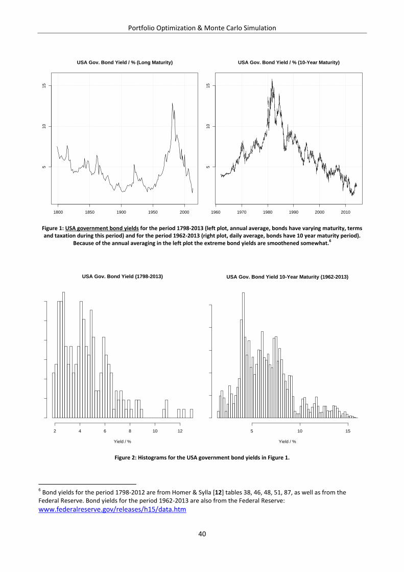
Portfolio Optimization & Monte Carlo Simulation
40
Figure 1: USA government bond yields for the period 1798-2013 (left plot, annual average, bonds have varying maturity, terms and taxation during this period) and for the period 1962-2013 (right plot, daily average, bonds have 10 year maturity period).
Because of the annual averaging in the left plot the extreme bond yields are smoothened somewhat.6
Figure 2: Histograms for the USA government bond yields in Figure 1.
6 Bond yields for the period 1798-2012 are from Homer & Sylla [12] tables 38, 46, 48, 51, 87, as well as from the
Federal Reserve. Bond yields for the period 1962-2013 are also from the Federal Reserve:
www.federalreserve.gov/releases/h15/data.htm
1800 1850 1900 1950 2000
510
15
USA Gov. Bond Yield / % (Long Maturity)
Year
Yie
ld / %
1960 1970 1980 1990 2000 20105
10
15
USA Gov. Bond Yield / % (10-Year Maturity)
Yie
ld / %
USA Gov. Bond Yield (1798-2013)
Yield / %
Density
2 4 6 8 10 12
0.0
00.0
50.1
00.1
50.2
00.2
50.3
0
USA Gov. Bond Yield 10-Year Maturity (1962-2013)
Yield / %
De
nsity
5 10 15
0.0
00
.05
0.1
00
.15
0.2
00
.25
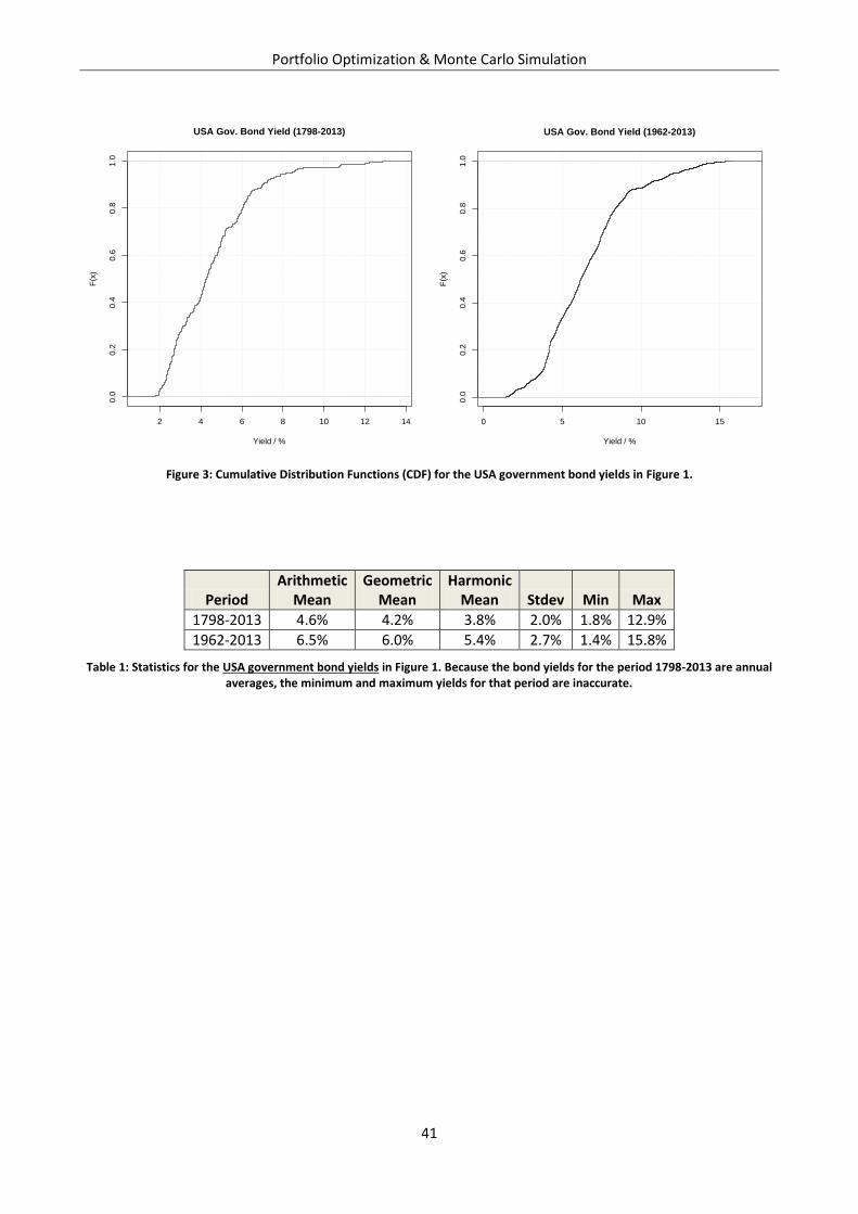
Portfolio Optimization & Monte Carlo Simulation
41
Figure 3: Cumulative Distribution Functions (CDF) for the USA government bond yields in Figure 1.
Period Arithmetic
Mean Geometric
Mean Harmonic
Mean Stdev Min Max
1798-2013 4.6% 4.2% 3.8% 2.0% 1.8% 12.9%
1962-2013 6.5% 6.0% 5.4% 2.7% 1.4% 15.8%
Table 1: Statistics for the USA government bond yields in Figure 1. Because the bond yields for the period 1798-2013 are annual averages, the minimum and maximum yields for that period are inaccurate.
2 4 6 8 10 12 14
0.0
0.2
0.4
0.6
0.8
1.0
USA Gov. Bond Yield (1798-2013)
Yield / %
F(x
)
0 5 10 15
0.0
0.2
0.4
0.6
0.8
1.0
USA Gov. Bond Yield (1962-2013)
Yield / %F
(x)
Portfolio Optimization & Monte Carlo Simulation
42
Figures & Tables
S&P 500
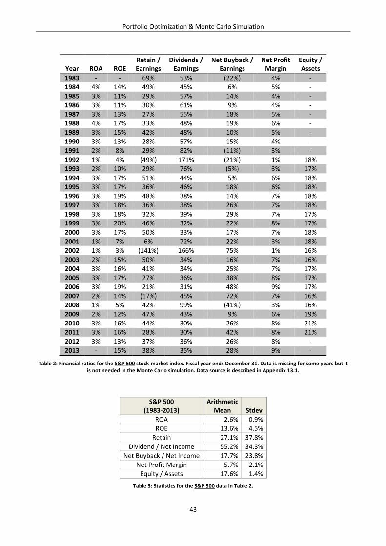
Portfolio Optimization & Monte Carlo Simulation
43
Year ROA ROE Retain / Earnings
Dividends / Earnings
Net Buyback / Earnings
Net Profit Margin
Equity / Assets
1983 - - 69% 53% (22%) 4% -
1984 4% 14% 49% 45% 6% 5% -
1985 3% 11% 29% 57% 14% 4% -
1986 3% 11% 30% 61% 9% 4% -
1987 3% 13% 27% 55% 18% 5% -
1988 4% 17% 33% 48% 19% 6% -
1989 3% 15% 42% 48% 10% 5% -
1990 3% 13% 28% 57% 15% 4% -
1991 2% 8% 29% 82% (11%) 3% -
1992 1% 4% (49%) 171% (21%) 1% 18%
1993 2% 10% 29% 76% (5%) 3% 17%
1994 3% 17% 51% 44% 5% 6% 18%
1995 3% 17% 36% 46% 18% 6% 18%
1996 3% 19% 48% 38% 14% 7% 18%
1997 3% 18% 36% 38% 26% 7% 18%
1998 3% 18% 32% 39% 29% 7% 17%
1999 3% 20% 46% 32% 22% 8% 17%
2000 3% 17% 50% 33% 17% 7% 18%
2001 1% 7% 6% 72% 22% 3% 18%
2002 1% 3% (141%) 166% 75% 1% 16%
2003 2% 15% 50% 34% 16% 7% 16%
2004 3% 16% 41% 34% 25% 7% 17%
2005 3% 17% 27% 36% 38% 8% 17%
2006 3% 19% 21% 31% 48% 9% 17%
2007 2% 14% (17%) 45% 72% 7% 16%
2008 1% 5% 42% 99% (41%) 3% 16%
2009 2% 12% 47% 43% 9% 6% 19%
2010 3% 16% 44% 30% 26% 8% 21%
2011 3% 16% 28% 30% 42% 8% 21%
2012 3% 13% 37% 36% 26% 8% -
2013 - 15% 38% 35% 28% 9% -
Table 2: Financial ratios for the S&P 500 stock-market index. Fiscal year ends December 31. Data is missing for some years but it is not needed in the Monte Carlo simulation. Data source is described in Appendix 13.1.
S&P 500 (1983-2013)
Arithmetic Mean Stdev
ROA 2.6% 0.9%
ROE 13.6% 4.5%
Retain 27.1% 37.8%
Dividend / Net Income 55.2% 34.3%
Net Buyback / Net Income 17.7% 23.8%
Net Profit Margin 5.7% 2.1%
Equity / Assets 17.6% 1.4%
Table 3: Statistics for the S&P 500 data in Table 2.
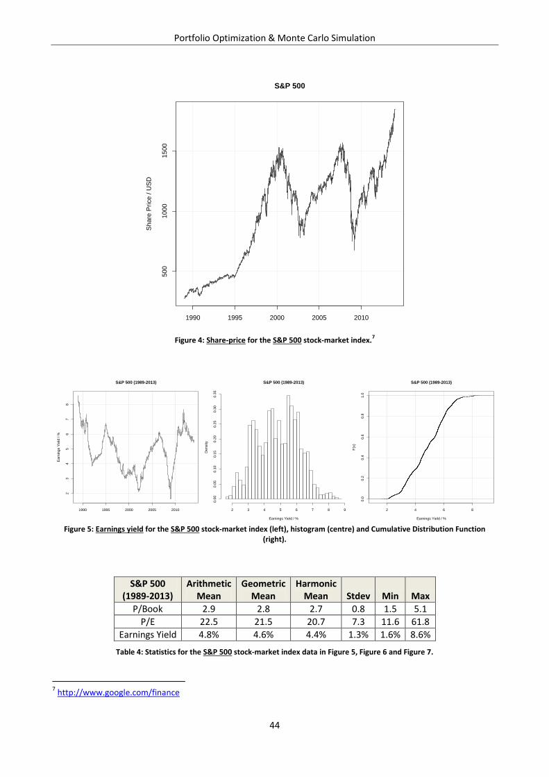
Portfolio Optimization & Monte Carlo Simulation
44
Figure 4: Share-price for the S&P 500 stock-market index.7
Figure 5: Earnings yield for the S&P 500 stock-market index (left), histogram (centre) and Cumulative Distribution Function
(right).
S&P 500 (1989-2013)
Arithmetic Mean
Geometric Mean
Harmonic Mean Stdev Min Max
P/Book 2.9 2.8 2.7 0.8 1.5 5.1
P/E 22.5 21.5 20.7 7.3 11.6 61.8
Earnings Yield 4.8% 4.6% 4.4% 1.3% 1.6% 8.6%
Table 4: Statistics for the S&P 500 stock-market index data in Figure 5, Figure 6 and Figure 7.
7 http://www.google.com/finance
1990 1995 2000 2005 2010
50
010
00
150
0
S&P 500
Sha
re P
rice / U
SD
1990 1995 2000 2005 2010
23
45
67
8
S&P 500 (1989-2013)
Earn
ings Y
ield
/ %
S&P 500 (1989-2013)
Earnings Yield / %
De
nsity
2 3 4 5 6 7 8 9
0.0
00
.05
0.1
00
.15
0.2
00
.25
0.3
00
.35
2 4 6 8
0.0
0.2
0.4
0.6
0.8
1.0
S&P 500 (1989-2013)
Earnings Yield / %
F(x
)
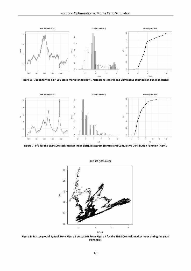
Portfolio Optimization & Monte Carlo Simulation
45
Figure 6: P/Book for the S&P 500 stock-market index (left), histogram (centre) and Cumulative Distribution Function (right).
Figure 7: P/E for the S&P 500 stock-market index (left), histogram (centre) and Cumulative Distribution Function (right).
Figure 8: Scatter-plot of P/Book from Figure 6 versus P/E from Figure 7 for the S&P 500 stock-market index during the years
1989-2013.
1990 1995 2000 2005 2010
23
45
S&P 500 (1989-2013)
P/B
oo
k
S&P 500 (1989-2013)
P/Book
Density
2 3 4 50.0
0.2
0.4
0.6
0.8
1.0
1 2 3 4 5
0.0
0.2
0.4
0.6
0.8
1.0
S&P 500 (1989-2013)
P/Book
F(x
)
1990 1995 2000 2005 2010
10
20
30
40
50
60
S&P 500 (1989-2013)
P/E
S&P 500 (1989-2013)
P/E
De
nsity
10 20 30 40 50 60
0.0
00
.02
0.0
40
.06
0.0
80
.10
10 20 30 40 50 60
0.0
0.2
0.4
0.6
0.8
1.0
S&P 500 (1989-2013)
P/E
F(x
)
2 3 4 5
10
20
30
40
50
60
S&P 500 (1989-2013)
P/Book
P/E
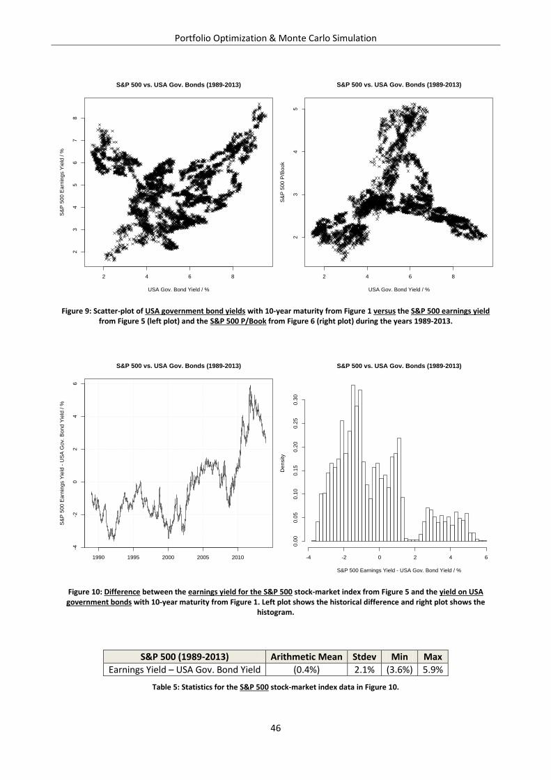
Portfolio Optimization & Monte Carlo Simulation
46
Figure 9: Scatter-plot of USA government bond yields with 10-year maturity from Figure 1 versus the S&P 500 earnings yield from Figure 5 (left plot) and the S&P 500 P/Book from Figure 6 (right plot) during the years 1989-2013.
Figure 10: Difference between the earnings yield for the S&P 500 stock-market index from Figure 5 and the yield on USA government bonds with 10-year maturity from Figure 1. Left plot shows the historical difference and right plot shows the
histogram.
S&P 500 (1989-2013) Arithmetic Mean Stdev Min Max
Earnings Yield – USA Gov. Bond Yield (0.4%) 2.1% (3.6%) 5.9%
Table 5: Statistics for the S&P 500 stock-market index data in Figure 10.
2 4 6 8
23
45
67
8
S&P 500 vs. USA Gov. Bonds (1989-2013)
USA Gov. Bond Yield / %
S&
P 5
00
Ea
rnin
gs Y
ield
/ %
2 4 6 8
23
45
S&P 500 vs. USA Gov. Bonds (1989-2013)
USA Gov. Bond Yield / %
S&
P 5
00
P/B
ook
1990 1995 2000 2005 2010
-4-2
02
46
S&P 500 vs. USA Gov. Bonds (1989-2013)
S&
P 5
00 E
arn
ings Y
ield
- U
SA
Gov. B
ond Y
ield
/ %
S&P 500 vs. USA Gov. Bonds (1989-2013)
S&P 500 Earnings Yield - USA Gov. Bond Yield / %
Density
-4 -2 0 2 4 6
0.0
00.0
50.1
00.1
50.2
00.2
50.3
0
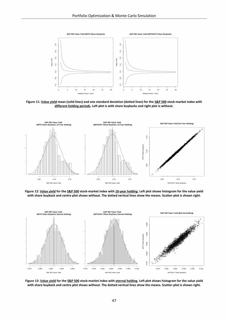
Portfolio Optimization & Monte Carlo Simulation
47
Figure 11: Value yield mean (solid lines) and one standard deviation (dotted lines) for the S&P 500 stock-market index with different holding periods. Left plot is with share buybacks and right plot is without.
Figure 12: Value yield for the S&P 500 stock-market index with 10-year holding. Left plot shows histogram for the value yield with share buyback and centre plot shows without. The dotted vertical lines show the means. Scatter-plot is shown right.
Figure 13: Value yield for the S&P 500 stock-market index with eternal holding. Left plot shows histogram for the value yield with share buyback and centre plot shows without. The dotted vertical lines show the means. Scatter-plot is shown right.
0 5 10 15 20 25 30
-0.1
0.0
0.1
0.2
0.3
0.4
0.5
S&P 500 Value Yield (WITH Share Buyback)
Holding Period / Years
Valu
e Y
ield
0 5 10 15 20 25 30
-0.1
0.0
0.1
0.2
0.3
0.4
0.5
S&P 500 Value Yield (WITHOUT Share Buyback)
Holding Period / Years
Valu
e Y
ield
S&P 500 Value Yield
(WITH Share Buyback, 10-Year Holding)
S&P 500 Value Yield
Density
0.05 0.10 0.15
05
10
15
S&P 500 Value Yield
(WITHOUT Share Buyback, 10-Year Holding)
S&P 500 Value Yield
Density
0.05 0.10 0.15
05
10
15
0.05 0.10 0.15
0.0
50.1
00.1
5
S&P 500 Value Yield (10-Year Holding)
WITHOUT Share Buyback
WIT
H S
hare
Buyback
S&P 500 Value Yield
(WITH Share Buyback, Eternal Holding)
S&P 500 Value Yield
Density
0.075 0.080 0.085 0.090 0.095
020
40
60
80
100
120
S&P 500 Value Yield
(WITHOUT Share Buyback, Eternal Holding)
S&P 500 Value Yield
Density
0.070 0.075 0.080 0.085 0.090 0.095 0.100
020
40
60
80
0.075 0.080 0.085 0.090 0.095 0.100
0.0
75
0.0
80
0.0
85
0.0
90
0.0
95
S&P 500 Value Yield (Eternal Holding)
WITHOUT Share Buyback
WIT
H S
hare
Buyback
Portfolio Optimization & Monte Carlo Simulation
48
Figures & Tables
Wal-Mart
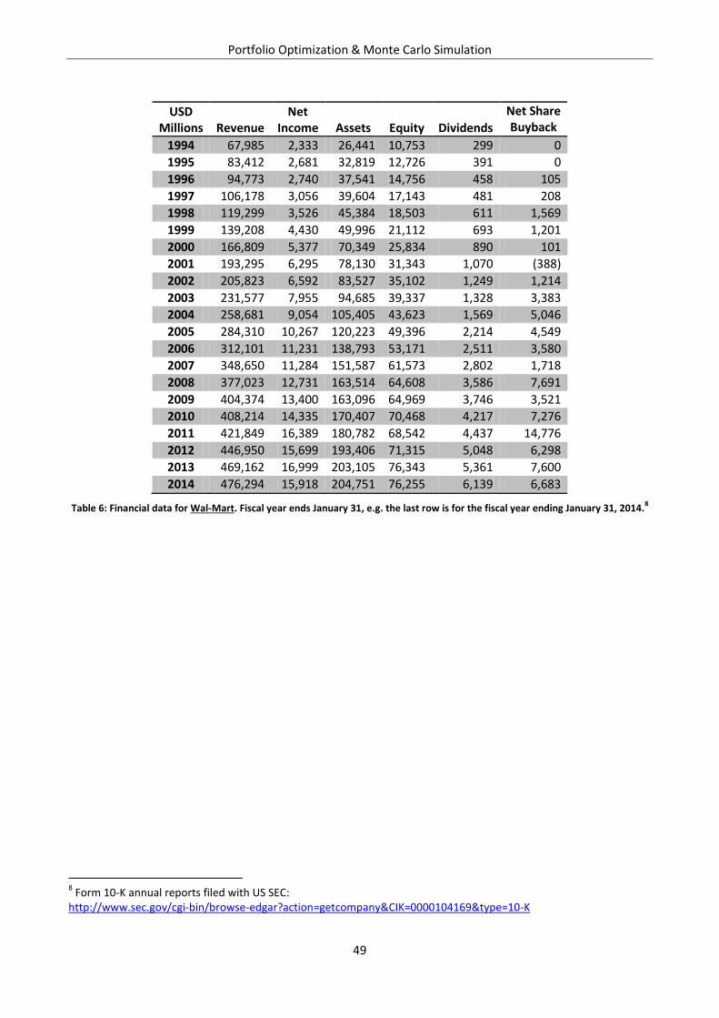
Portfolio Optimization & Monte Carlo Simulation
49
USD Millions Revenue
Net Income Assets Equity Dividends
Net Share Buyback
1994 67,985 2,333 26,441 10,753 299 0
1995 83,412 2,681 32,819 12,726 391 0
1996 94,773 2,740 37,541 14,756 458 105
1997 106,178 3,056 39,604 17,143 481 208
1998 119,299 3,526 45,384 18,503 611 1,569
1999 139,208 4,430 49,996 21,112 693 1,201
2000 166,809 5,377 70,349 25,834 890 101
2001 193,295 6,295 78,130 31,343 1,070 (388)
2002 205,823 6,592 83,527 35,102 1,249 1,214
2003 231,577 7,955 94,685 39,337 1,328 3,383
2004 258,681 9,054 105,405 43,623 1,569 5,046
2005 284,310 10,267 120,223 49,396 2,214 4,549
2006 312,101 11,231 138,793 53,171 2,511 3,580
2007 348,650 11,284 151,587 61,573 2,802 1,718
2008 377,023 12,731 163,514 64,608 3,586 7,691
2009 404,374 13,400 163,096 64,969 3,746 3,521
2010 408,214 14,335 170,407 70,468 4,217 7,276
2011 421,849 16,389 180,782 68,542 4,437 14,776
2012 446,950 15,699 193,406 71,315 5,048 6,298
2013 469,162 16,999 203,105 76,343 5,361 7,600
2014 476,294 15,918 204,751 76,255 6,139 6,683
Table 6: Financial data for Wal-Mart. Fiscal year ends January 31, e.g. the last row is for the fiscal year ending January 31, 2014.8
8 Form 10-K annual reports filed with US SEC:
http://www.sec.gov/cgi-bin/browse-edgar?action=getcompany&CIK=0000104169&type=10-K
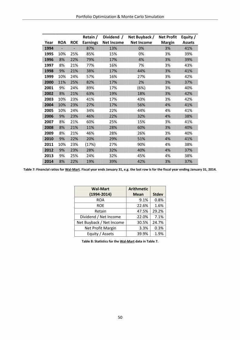
Portfolio Optimization & Monte Carlo Simulation
50
Year ROA ROE Retain / Earnings
Dividend / Net Income
Net Buyback / Net Income
Net Profit Margin
Equity / Assets
1994 - - 87% 13% 0% 3% 41%
1995 10% 25% 85% 15% 0% 3% 39%
1996 8% 22% 79% 17% 4% 3% 39%
1997 8% 21% 77% 16% 7% 3% 43%
1998 9% 21% 38% 17% 44% 3% 41%
1999 10% 24% 57% 16% 27% 3% 42%
2000 11% 25% 82% 17% 2% 3% 37%
2001 9% 24% 89% 17% (6%) 3% 40%
2002 8% 21% 63% 19% 18% 3% 42%
2003 10% 23% 41% 17% 43% 3% 42%
2004 10% 23% 27% 17% 56% 4% 41%
2005 10% 24% 34% 22% 44% 4% 41%
2006 9% 23% 46% 22% 32% 4% 38%
2007 8% 21% 60% 25% 15% 3% 41%
2008 8% 21% 11% 28% 60% 3% 40%
2009 8% 21% 46% 28% 26% 3% 40%
2010 9% 22% 20% 29% 51% 4% 41%
2011 10% 23% (17%) 27% 90% 4% 38%
2012 9% 23% 28% 32% 40% 4% 37%
2013 9% 25% 24% 32% 45% 4% 38%
2014 8% 22% 19% 39% 42% 3% 37%
Table 7: Financial ratios for Wal-Mart. Fiscal year ends January 31, e.g. the last row is for the fiscal year ending January 31, 2014.
Wal-Mart (1994-2014)
Arithmetic Mean Stdev
ROA 9.1% 0.8%
ROE 22.6% 1.6%
Retain 47.5% 29.2%
Dividend / Net Income 22.0% 7.1%
Net Buyback / Net Income 30.5% 24.7%
Net Profit Margin 3.3% 0.3%
Equity / Assets 39.9% 1.9%
Table 8: Statistics for the Wal-Mart data in Table 7.
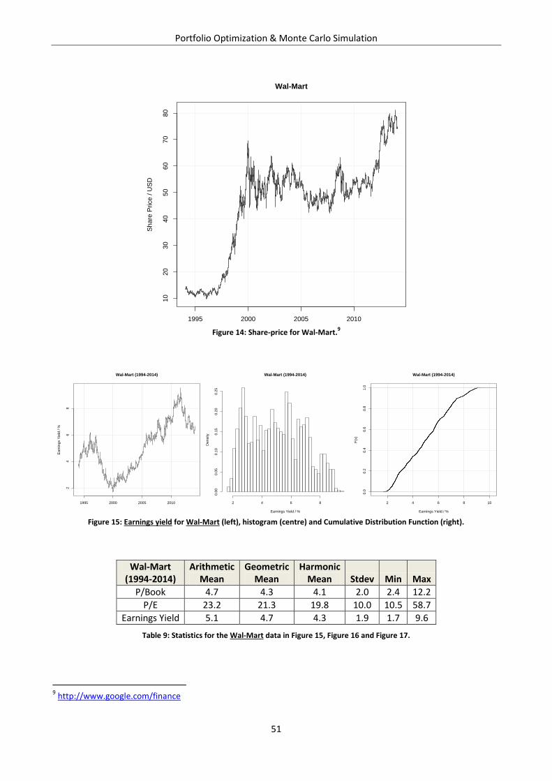
Portfolio Optimization & Monte Carlo Simulation
51
Figure 14: Share-price for Wal-Mart.
9
Figure 15: Earnings yield for Wal-Mart (left), histogram (centre) and Cumulative Distribution Function (right).
Wal-Mart (1994-2014)
Arithmetic Mean
Geometric Mean
Harmonic Mean Stdev Min Max
P/Book 4.7 4.3 4.1 2.0 2.4 12.2
P/E 23.2 21.3 19.8 10.0 10.5 58.7
Earnings Yield 5.1 4.7 4.3 1.9 1.7 9.6
Table 9: Statistics for the Wal-Mart data in Figure 15, Figure 16 and Figure 17.
9 http://www.google.com/finance
1995 2000 2005 2010
10
20
30
40
50
60
70
80
Wal-Mart
Sh
are
Price
/ U
SD
1995 2000 2005 2010
24
68
Wal-Mart (1994-2014)
Ea
rnin
gs Y
ield
/ %
Wal-Mart (1994-2014)
Earnings Yield / %
De
nsity
2 4 6 8
0.0
00
.05
0.1
00
.15
0.2
00
.25
2 4 6 8 10
0.0
0.2
0.4
0.6
0.8
1.0
Wal-Mart (1994-2014)
Earnings Yield / %
F(x
)
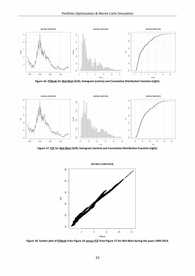
Portfolio Optimization & Monte Carlo Simulation
52
Figure 16: P/Book for Wal-Mart (left), histogram (centre) and Cumulative Distribution Function (right).
Figure 17: P/E for Wal-Mart (left), histogram (centre) and Cumulative Distribution Function (right).
Figure 18: Scatter-plot of P/Book from Figure 16 versus P/E from Figure 17 for Wal-Mart during the years 1994-2014.
1995 2000 2005 2010
46
81
01
2
Wal-Mart (1994-2014)
P/B
oo
k
Wal-Mart (1994-2014)
P/Book
De
nsity
2 4 6 8 10 12
0.0
0.1
0.2
0.3
0.4
0.5
2 4 6 8 10 12
0.0
0.2
0.4
0.6
0.8
1.0
Wal-Mart (1994-2014)
P/Book
F(x
)
1995 2000 2005 2010
10
20
30
40
50
60
Wal-Mart (1994-2014)
P/E
Wal-Mart (1994-2014)
P/E
De
nsity
10 20 30 40 50 60
0.0
00
.02
0.0
40
.06
0.0
8
10 20 30 40 50 60
0.0
0.2
0.4
0.6
0.8
1.0
Wal-Mart (1994-2014)
P/E
F(x
)
4 6 8 10 12
10
20
30
40
50
60
Wal-Mart (1994-2014)
P/Book
P/E
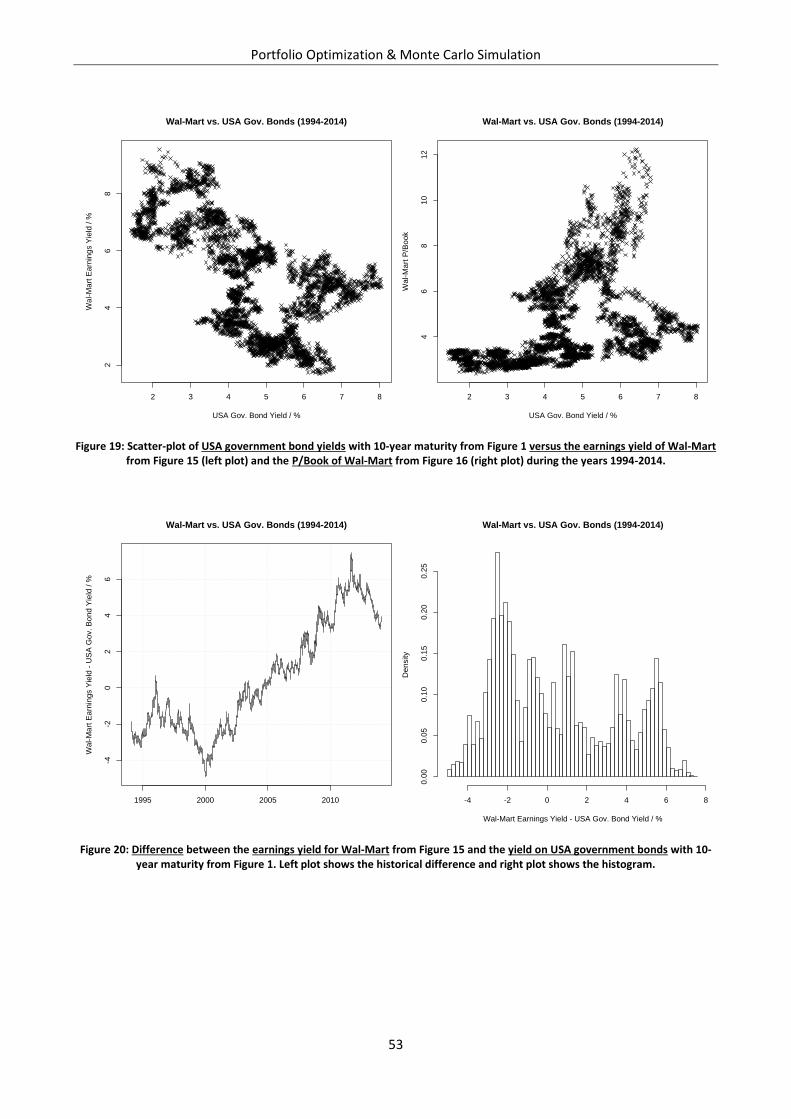
Portfolio Optimization & Monte Carlo Simulation
53
Figure 19: Scatter-plot of USA government bond yields with 10-year maturity from Figure 1 versus the earnings yield of Wal-Mart from Figure 15 (left plot) and the P/Book of Wal-Mart from Figure 16 (right plot) during the years 1994-2014.
Figure 20: Difference between the earnings yield for Wal-Mart from Figure 15 and the yield on USA government bonds with 10-year maturity from Figure 1. Left plot shows the historical difference and right plot shows the histogram.
2 3 4 5 6 7 8
24
68
Wal-Mart vs. USA Gov. Bonds (1994-2014)
USA Gov. Bond Yield / %
Wal-M
art
Earn
ings Y
ield
/ %
2 3 4 5 6 7 8
46
810
12
Wal-Mart vs. USA Gov. Bonds (1994-2014)
USA Gov. Bond Yield / %
Wal-M
art
P/B
ook
1995 2000 2005 2010
-4-2
02
46
Wal-Mart vs. USA Gov. Bonds (1994-2014)
Wal-M
art
Earn
ings Y
ield
- U
SA
Gov. B
ond Y
ield
/ %
Wal-Mart vs. USA Gov. Bonds (1994-2014)
Wal-Mart Earnings Yield - USA Gov. Bond Yield / %
Density
-4 -2 0 2 4 6 8
0.0
00.0
50.1
00.1
50.2
00.2
5
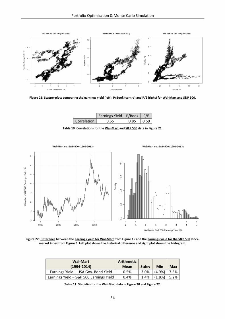
Portfolio Optimization & Monte Carlo Simulation
54
Figure 21: Scatter-plots comparing the earnings yield (left), P/Book (centre) and P/E (right) for Wal-Mart and S&P 500.
Earnings Yield P/Book P/E
Correlation 0.65 0.85 0.59
Table 10: Correlations for the Wal-Mart and S&P 500 data in Figure 21.
Figure 22: Difference between the earnings yield for Wal-Mart from Figure 15 and the earnings yield for the S&P 500 stock-market index from Figure 5. Left plot shows the historical difference and right plot shows the histogram.
Wal-Mart (1994-2014)
Arithmetic Mean Stdev Min Max
Earnings Yield – USA Gov. Bond Yield 0.5% 3.0% (4.9%) 7.5%
Earnings Yield – S&P 500 Earnings Yield 0.4% 1.4% (1.8%) 5.2%
Table 11: Statistics for the Wal-Mart data in Figure 20 and Figure 22.
2 3 4 5 6 7
24
68
Wal-Mart vs. S&P 500 (1994-2013)
S&P 500 Earnings Yield / %
Wa
l-M
art
Ea
rnin
gs Y
ield
/ %
2 3 4 5
46
81
01
2
Wal-Mart vs. S&P 500 (1994-2013)
S&P 500 P/Book
Wa
l-M
art
P/B
oo
k
20 30 40 50 60
10
20
30
40
50
60
Wal-Mart vs. S&P 500 (1994-2013)
S&P 500 P/E
Wa
l-M
art
P/E
1995 2000 2005 2010
-2-1
01
23
45
Wal-Mart vs. S&P 500 (1994-2013)
Wal-M
art
- S
&P
500 E
arn
ings Y
ield
/ %
Wal-Mart vs. S&P 500 (1994-2013)
Wal-Mart - S&P 500 Earnings Yield / %
Density
-2 -1 0 1 2 3 4 5
0.0
0.1
0.2
0.3
0.4
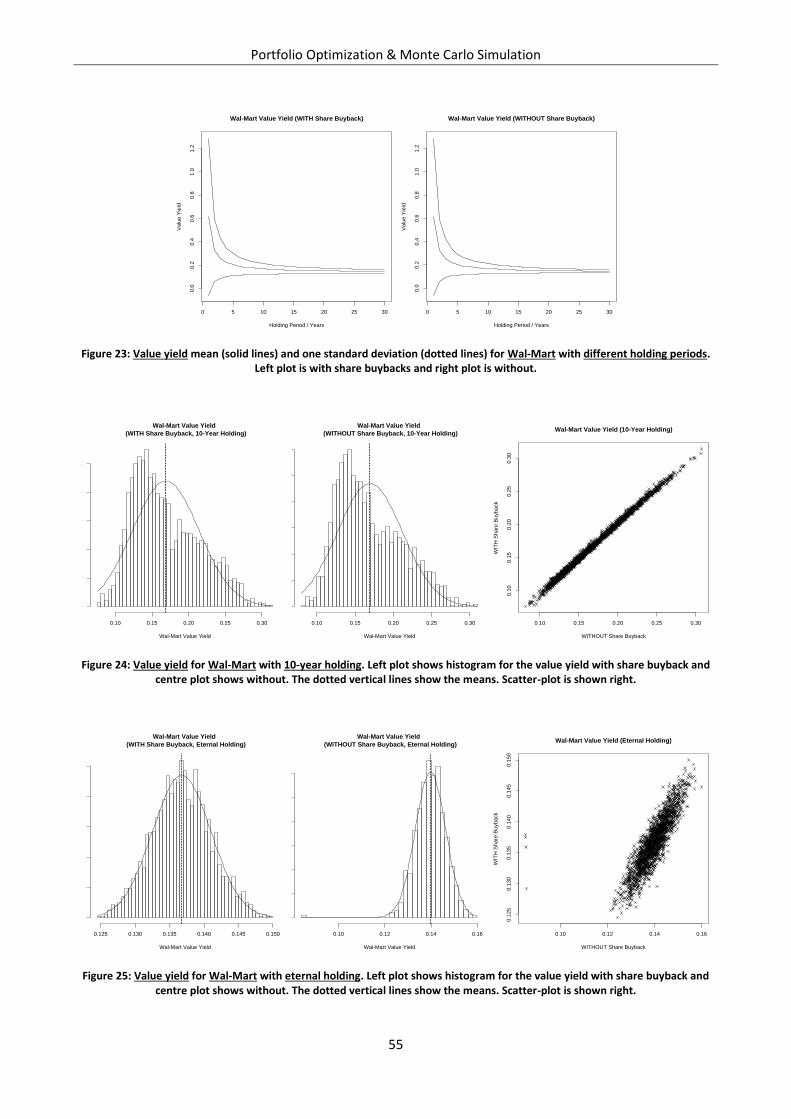
Portfolio Optimization & Monte Carlo Simulation
55
Figure 23: Value yield mean (solid lines) and one standard deviation (dotted lines) for Wal-Mart with different holding periods. Left plot is with share buybacks and right plot is without.
Figure 24: Value yield for Wal-Mart with 10-year holding. Left plot shows histogram for the value yield with share buyback and centre plot shows without. The dotted vertical lines show the means. Scatter-plot is shown right.
Figure 25: Value yield for Wal-Mart with eternal holding. Left plot shows histogram for the value yield with share buyback and centre plot shows without. The dotted vertical lines show the means. Scatter-plot is shown right.
0 5 10 15 20 25 30
0.0
0.2
0.4
0.6
0.8
1.0
1.2
Wal-Mart Value Yield (WITH Share Buyback)
Holding Period / Years
Valu
e Y
ield
0 5 10 15 20 25 30
0.0
0.2
0.4
0.6
0.8
1.0
1.2
Wal-Mart Value Yield (WITHOUT Share Buyback)
Holding Period / Years
Valu
e Y
ield
Wal-Mart Value Yield
(WITH Share Buyback, 10-Year Holding)
Wal-Mart Value Yield
Density
0.10 0.15 0.20 0.25 0.30
02
46
810
Wal-Mart Value Yield
(WITHOUT Share Buyback, 10-Year Holding)
Wal-Mart Value Yield
Density
0.10 0.15 0.20 0.25 0.30
02
46
810
12
0.10 0.15 0.20 0.25 0.30
0.1
00.1
50.2
00.2
50.3
0
Wal-Mart Value Yield (10-Year Holding)
WITHOUT Share Buyback
WIT
H S
hare
Buyback
Wal-Mart Value Yield
(WITH Share Buyback, Eternal Holding)
Wal-Mart Value Yield
Density
0.125 0.130 0.135 0.140 0.145 0.150
020
40
60
80
100
Wal-Mart Value Yield
(WITHOUT Share Buyback, Eternal Holding)
Wal-Mart Value Yield
Density
0.10 0.12 0.14 0.16
010
20
30
40
50
60
0.10 0.12 0.14 0.16
0.1
25
0.1
30
0.1
35
0.1
40
0.1
45
0.1
50
Wal-Mart Value Yield (Eternal Holding)
WITHOUT Share Buyback
WIT
H S
hare
Buyback
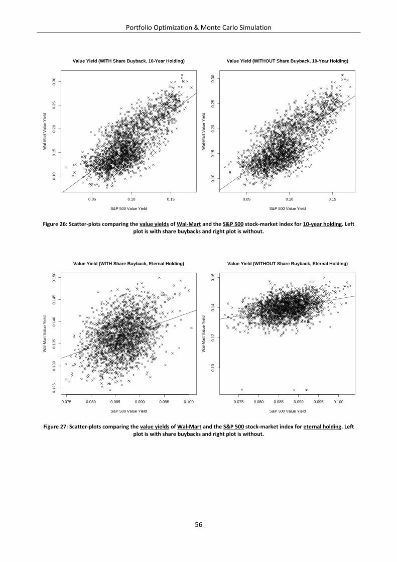
Portfolio Optimization & Monte Carlo Simulation
56
Figure 26: Scatter-plots comparing the value yields of Wal-Mart and the S&P 500 stock-market index for 10-year holding. Left plot is with share buybacks and right plot is without.
Figure 27: Scatter-plots comparing the value yields of Wal-Mart and the S&P 500 stock-market index for eternal holding. Left plot is with share buybacks and right plot is without.
0.05 0.10 0.15
0.1
00.1
50.2
00.2
50.3
0
Value Yield (WITH Share Buyback, 10-Year Holding)
S&P 500 Value Yield
Wal-M
art
Va
lue
Yie
ld
0.05 0.10 0.15
0.1
00
.15
0.2
00
.25
0.3
0
Value Yield (WITHOUT Share Buyback, 10-Year Holding)
S&P 500 Value Yield
Wal-M
art
Va
lue
Yie
ld
0.075 0.080 0.085 0.090 0.095 0.100
0.1
25
0.1
30
0.1
35
0.1
40
0.1
45
0.1
50
Value Yield (WITH Share Buyback, Eternal Holding)
S&P 500 Value Yield
Wal-M
art
Valu
e Y
ield
0.075 0.080 0.085 0.090 0.095 0.100
0.1
00.1
20.1
40.1
6
Value Yield (WITHOUT Share Buyback, Eternal Holding)
S&P 500 Value Yield
Wal-M
art
Valu
e Y
ield
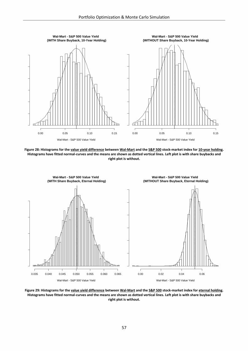
Portfolio Optimization & Monte Carlo Simulation
57
Figure 28: Histograms for the value yield difference between Wal-Mart and the S&P 500 stock-market index for 10-year holding. Histograms have fitted normal-curves and the means are shown as dotted vertical lines. Left plot is with share buybacks and
right plot is without.
Figure 29: Histograms for the value yield difference between Wal-Mart and the S&P 500 stock-market index for eternal holding. Histograms have fitted normal-curves and the means are shown as dotted vertical lines. Left plot is with share buybacks and
right plot is without.
Wal-Mart - S&P 500 Value Yield
(WITH Share Buyback, 10-Year Holding)
Wal-Mart - S&P 500 Value Yield
Density
0.00 0.05 0.10 0.15
02
46
810
12
Wal-Mart - S&P 500 Value Yield
(WITHOUT Share Buyback, 10-Year Holding)
Wal-Mart - S&P 500 Value Yield
Density
0.00 0.05 0.10 0.15
02
46
810
12
Wal-Mart - S&P 500 Value Yield
(WITH Share Buyback, Eternal Holding)
Wal-Mart - S&P 500 Value Yield
Density
0.035 0.040 0.045 0.050 0.055 0.060 0.065
020
40
60
80
Wal-Mart - S&P 500 Value Yield
(WITHOUT Share Buyback, Eternal Holding)
Wal-Mart - S&P 500 Value Yield
Density
0.00 0.02 0.04 0.06
010
20
30
40
50
60
Portfolio Optimization & Monte Carlo Simulation
58
Figures & Tables
Coca-Cola
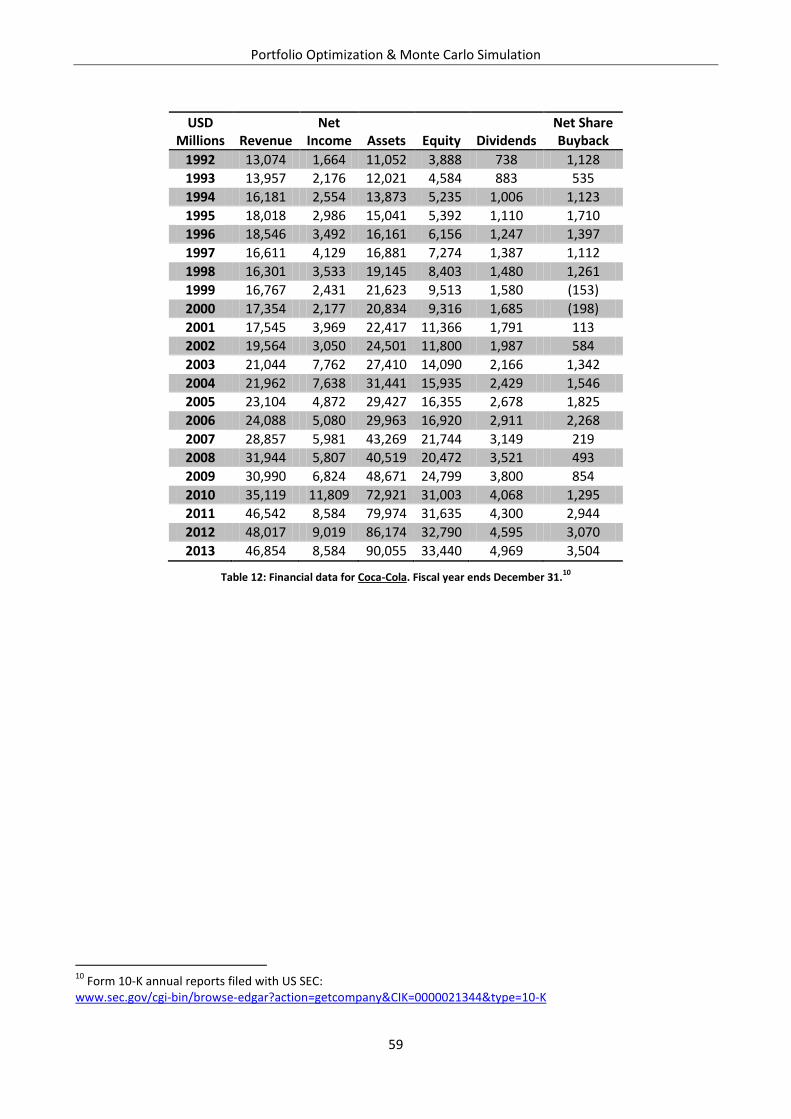
Portfolio Optimization & Monte Carlo Simulation
59
USD Millions Revenue
Net Income Assets Equity Dividends
Net Share Buyback
1992 13,074 1,664 11,052 3,888 738 1,128
1993 13,957 2,176 12,021 4,584 883 535
1994 16,181 2,554 13,873 5,235 1,006 1,123
1995 18,018 2,986 15,041 5,392 1,110 1,710
1996 18,546 3,492 16,161 6,156 1,247 1,397
1997 16,611 4,129 16,881 7,274 1,387 1,112
1998 16,301 3,533 19,145 8,403 1,480 1,261
1999 16,767 2,431 21,623 9,513 1,580 (153)
2000 17,354 2,177 20,834 9,316 1,685 (198)
2001 17,545 3,969 22,417 11,366 1,791 113
2002 19,564 3,050 24,501 11,800 1,987 584
2003 21,044 7,762 27,410 14,090 2,166 1,342
2004 21,962 7,638 31,441 15,935 2,429 1,546
2005 23,104 4,872 29,427 16,355 2,678 1,825
2006 24,088 5,080 29,963 16,920 2,911 2,268
2007 28,857 5,981 43,269 21,744 3,149 219
2008 31,944 5,807 40,519 20,472 3,521 493
2009 30,990 6,824 48,671 24,799 3,800 854
2010 35,119 11,809 72,921 31,003 4,068 1,295
2011 46,542 8,584 79,974 31,635 4,300 2,944
2012 48,017 9,019 86,174 32,790 4,595 3,070
2013 46,854 8,584 90,055 33,440 4,969 3,504
Table 12: Financial data for Coca-Cola. Fiscal year ends December 31.10
10
Form 10-K annual reports filed with US SEC: www.sec.gov/cgi-bin/browse-edgar?action=getcompany&CIK=0000021344&type=10-K
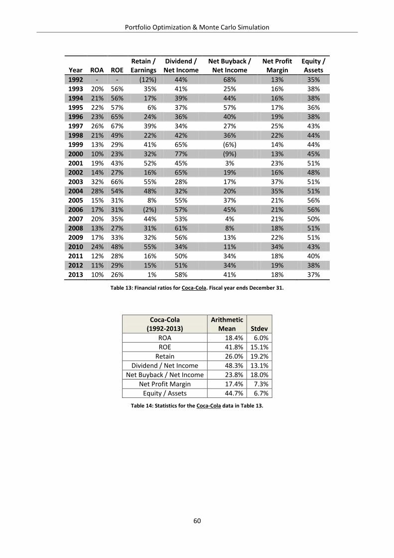
Portfolio Optimization & Monte Carlo Simulation
60
Year ROA ROE Retain / Earnings
Dividend / Net Income
Net Buyback / Net Income
Net Profit Margin
Equity / Assets
1992 - - (12%) 44% 68% 13% 35%
1993 20% 56% 35% 41% 25% 16% 38%
1994 21% 56% 17% 39% 44% 16% 38%
1995 22% 57% 6% 37% 57% 17% 36%
1996 23% 65% 24% 36% 40% 19% 38%
1997 26% 67% 39% 34% 27% 25% 43%
1998 21% 49% 22% 42% 36% 22% 44%
1999 13% 29% 41% 65% (6%) 14% 44%
2000 10% 23% 32% 77% (9%) 13% 45%
2001 19% 43% 52% 45% 3% 23% 51%
2002 14% 27% 16% 65% 19% 16% 48%
2003 32% 66% 55% 28% 17% 37% 51%
2004 28% 54% 48% 32% 20% 35% 51%
2005 15% 31% 8% 55% 37% 21% 56%
2006 17% 31% (2%) 57% 45% 21% 56%
2007 20% 35% 44% 53% 4% 21% 50%
2008 13% 27% 31% 61% 8% 18% 51%
2009 17% 33% 32% 56% 13% 22% 51%
2010 24% 48% 55% 34% 11% 34% 43%
2011 12% 28% 16% 50% 34% 18% 40%
2012 11% 29% 15% 51% 34% 19% 38%
2013 10% 26% 1% 58% 41% 18% 37%
Table 13: Financial ratios for Coca-Cola. Fiscal year ends December 31.
Coca-Cola (1992-2013)
Arithmetic Mean Stdev
ROA 18.4% 6.0%
ROE 41.8% 15.1%
Retain 26.0% 19.2%
Dividend / Net Income 48.3% 13.1%
Net Buyback / Net Income 23.8% 18.0%
Net Profit Margin 17.4% 7.3%
Equity / Assets 44.7% 6.7%
Table 14: Statistics for the Coca-Cola data in Table 13.
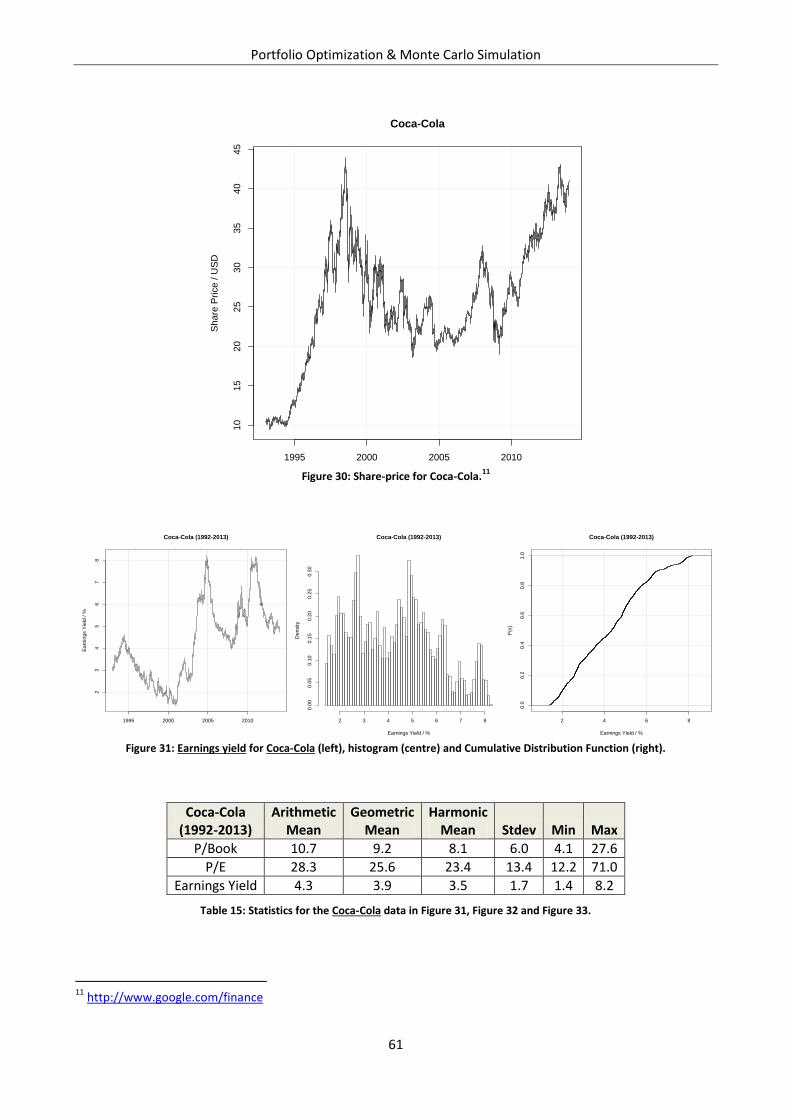
Portfolio Optimization & Monte Carlo Simulation
61
Figure 30: Share-price for Coca-Cola.
11
Figure 31: Earnings yield for Coca-Cola (left), histogram (centre) and Cumulative Distribution Function (right).
Coca-Cola (1992-2013)
Arithmetic Mean
Geometric Mean
Harmonic Mean Stdev Min Max
P/Book 10.7 9.2 8.1 6.0 4.1 27.6
P/E 28.3 25.6 23.4 13.4 12.2 71.0
Earnings Yield 4.3 3.9 3.5 1.7 1.4 8.2
Table 15: Statistics for the Coca-Cola data in Figure 31, Figure 32 and Figure 33.
11
http://www.google.com/finance
1995 2000 2005 2010
10
15
20
25
30
35
40
45
Coca-Cola
Sh
are
Price
/ U
SD
1995 2000 2005 2010
23
45
67
8
Coca-Cola (1992-2013)
Ea
rnin
gs Y
ield
/ %
Coca-Cola (1992-2013)
Earnings Yield / %
De
nsity
2 3 4 5 6 7 8
0.0
00
.05
0.1
00
.15
0.2
00
.25
0.3
0
2 4 6 8
0.0
0.2
0.4
0.6
0.8
1.0
Coca-Cola (1992-2013)
Earnings Yield / %
F(x
)
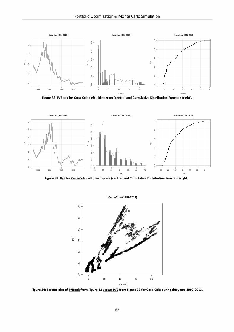
Portfolio Optimization & Monte Carlo Simulation
62
Figure 32: P/Book for Coca-Cola (left), histogram (centre) and Cumulative Distribution Function (right).
Figure 33: P/E for Coca-Cola (left), histogram (centre) and Cumulative Distribution Function (right).
Figure 34: Scatter-plot of P/Book from Figure 32 versus P/E from Figure 33 for Coca-Cola during the years 1992-2013.
1995 2000 2005 2010
51
01
52
02
5
Coca-Cola (1992-2013)
P/B
oo
k
Coca-Cola (1992-2013)
P/Book
De
nsity
5 10 15 20 25
0.0
00
.05
0.1
00
.15
0.2
00
.25
5 10 15 20 25 30
0.0
0.2
0.4
0.6
0.8
1.0
Coca-Cola (1992-2013)
P/Book
F(x
)
1995 2000 2005 2010
10
20
30
40
50
60
70
Coca-Cola (1992-2013)
P/E
Coca-Cola (1992-2013)
P/E
De
nsity
10 20 30 40 50 60 70
0.0
00
.01
0.0
20
.03
0.0
40
.05
0.0
6
10 20 30 40 50 60 70
0.0
0.2
0.4
0.6
0.8
1.0
Coca-Cola (1992-2013)
P/E
F(x
)
5 10 15 20 25
10
20
30
40
50
60
70
Coca-Cola (1992-2013)
P/Book
P/E
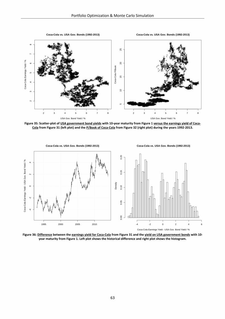
Portfolio Optimization & Monte Carlo Simulation
63
Figure 35: Scatter-plot of USA government bond yields with 10-year maturity from Figure 1 versus the earnings yield of Coca-
Cola from Figure 31 (left plot) and the P/Book of Coca-Cola from Figure 32 (right plot) during the years 1992-2013.
Figure 36: Difference between the earnings yield for Coca-Cola from Figure 31 and the yield on USA government bonds with 10-
year maturity from Figure 1. Left plot shows the historical difference and right plot shows the histogram.
2 3 4 5 6 7 8
23
45
67
8
Coca-Cola vs. USA Gov. Bonds (1992-2013)
USA Gov. Bond Yield / %
Coca-C
ola
Earn
ings Y
ield
/ %
2 3 4 5 6 7 8
510
15
20
25
Coca-Cola vs. USA Gov. Bonds (1992-2013)
USA Gov. Bond Yield / %
Coca-C
ola
P/B
oo
k
1995 2000 2005 2010
-4-2
02
4
Coca-Cola vs. USA Gov. Bonds (1992-2013)
Coca-C
ola
Earn
ings Y
ield
- U
SA
Gov. B
ond Y
ield
/ %
Coca-Cola vs. USA Gov. Bonds (1992-2013)
Coca-Cola Earnings Yield - USA Gov. Bond Yield / %
Density
-4 -2 0 2 4 6
0.0
00.0
50.1
00.1
50.2
0
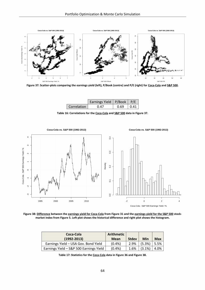
Portfolio Optimization & Monte Carlo Simulation
64
Figure 37: Scatter-plots comparing the earnings yield (left), P/Book (centre) and P/E (right) for Coca-Cola and S&P 500.
Earnings Yield P/Book P/E
Correlation 0.47 0.69 0.41
Table 16: Correlations for the Coca-Cola and S&P 500 data in Figure 37.
Figure 38: Difference between the earnings yield for Coca-Cola from Figure 31 and the earnings yield for the S&P 500 stock-market index from Figure 5. Left plot shows the historical difference and right plot shows the histogram.
Coca-Cola (1992-2013)
Arithmetic Mean Stdev Min Max
Earnings Yield – USA Gov. Bond Yield (0.4%) 2.9% (5.3%) 5.5%
Earnings Yield – S&P 500 Earnings Yield (0.4%) 1.6% (3.1%) 4.0%
Table 17: Statistics for the Coca-Cola data in Figure 36 and Figure 38.
2 3 4 5 6 7
23
45
67
8
Coca-Cola vs. S&P 500 (1992-2013)
S&P 500 Earnings Yield / %
Co
ca
-Co
la E
arn
ing
s Y
ield
/ %
2 3 4 5
51
01
52
02
5
Coca-Cola vs. S&P 500 (1992-2013)
S&P 500 P/Book
Co
ca
-Co
la P
/Bo
ok
20 30 40 50 60
10
20
30
40
50
60
70
Coca-Cola vs. S&P 500 (1992-2013)
S&P 500 P/E
Co
ca
-Co
la P
/E
1995 2000 2005 2010
-3-2
-10
12
34
Coca-Cola vs. S&P 500 (1992-2013)
Coca-C
ola
- S
&P
500 E
arn
ings Y
ield
/ %
Coca-Cola vs. S&P 500 (1992-2013)
Coca-Cola - S&P 500 Earnings Yield / %
Density
-2 0 2 4
0.0
0.1
0.2
0.3
0.4
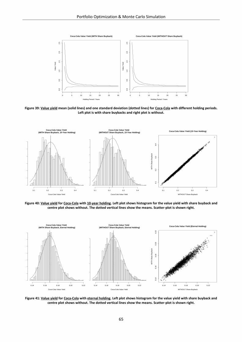
Portfolio Optimization & Monte Carlo Simulation
65
Figure 39: Value yield mean (solid lines) and one standard deviation (dotted lines) for Coca-Cola with different holding periods. Left plot is with share buybacks and right plot is without.
Figure 40: Value yield for Coca-Cola with 10-year holding. Left plot shows histogram for the value yield with share buyback and centre plot shows without. The dotted vertical lines show the means. Scatter-plot is shown right.
Figure 41: Value yield for Coca-Cola with eternal holding. Left plot shows histogram for the value yield with share buyback and centre plot shows without. The dotted vertical lines show the means. Scatter-plot is shown right.
0 5 10 15 20 25 30
0.0
0.5
1.0
1.5
2.0
2.5
Coca-Cola Value Yield (WITH Share Buyback)
Holding Period / Years
Valu
e Y
ield
0 5 10 15 20 25 30
0.0
0.5
1.0
1.5
2.0
2.5
Coca-Cola Value Yield (WITHOUT Share Buyback)
Holding Period / Years
Valu
e Y
ield
Coca-Cola Value Yield
(WITH Share Buyback, 10-Year Holding)
Coca-Cola Value Yield
Density
0.1 0.2 0.3 0.4
01
23
45
6
Coca-Cola Value Yield
(WITHOUT Share Buyback, 10-Year Holding)
Coca-Cola Value Yield
Density
0.1 0.2 0.3 0.4
01
23
45
6
0.1 0.2 0.3 0.4
0.1
0.2
0.3
0.4
Coca-Cola Value Yield (10-Year Holding)
WITHOUT Share Buyback
WIT
H S
hare
Buyback
Coca-Cola Value Yield
(WITH Share Buyback, Eternal Holding)
Coca-Cola Value Yield
Density
0.14 0.16 0.18 0.20 0.22
05
10
15
20
25
30
35
Coca-Cola Value Yield
(WITHOUT Share Buyback, Eternal Holding)
Coca-Cola Value Yield
Density
0.14 0.16 0.18 0.20 0.22
05
10
15
20
25
0.14 0.16 0.18 0.20 0.22
0.1
40.1
60.1
80.2
00.2
2
Coca-Cola Value Yield (Eternal Holding)
WITHOUT Share Buyback
WIT
H S
hare
Buyback
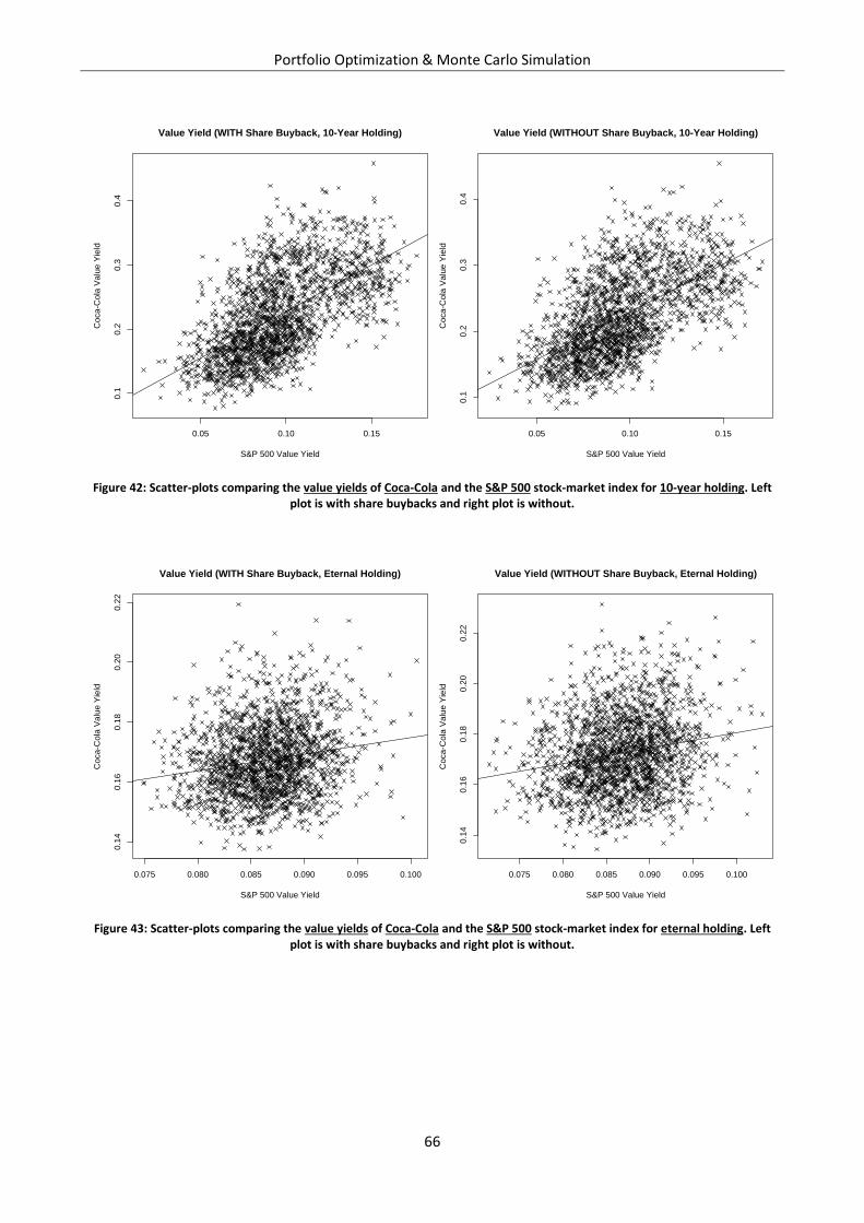
Portfolio Optimization & Monte Carlo Simulation
66
Figure 42: Scatter-plots comparing the value yields of Coca-Cola and the S&P 500 stock-market index for 10-year holding. Left plot is with share buybacks and right plot is without.
Figure 43: Scatter-plots comparing the value yields of Coca-Cola and the S&P 500 stock-market index for eternal holding. Left plot is with share buybacks and right plot is without.
0.05 0.10 0.15
0.1
0.2
0.3
0.4
Value Yield (WITH Share Buyback, 10-Year Holding)
S&P 500 Value Yield
Coca-C
ola
Valu
e Y
ield
0.05 0.10 0.15
0.1
0.2
0.3
0.4
Value Yield (WITHOUT Share Buyback, 10-Year Holding)
S&P 500 Value Yield
Coca-C
ola
Valu
e Y
ield
0.075 0.080 0.085 0.090 0.095 0.100
0.1
40.1
60.1
80.2
00.2
2
Value Yield (WITH Share Buyback, Eternal Holding)
S&P 500 Value Yield
Coca-C
ola
Valu
e Y
ield
0.075 0.080 0.085 0.090 0.095 0.100
0.1
40.1
60.1
80.2
00.2
2
Value Yield (WITHOUT Share Buyback, Eternal Holding)
S&P 500 Value Yield
Coca-C
ola
Valu
e Y
ield
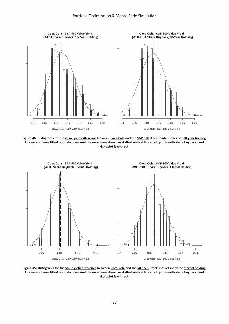
Portfolio Optimization & Monte Carlo Simulation
67
Figure 44: Histograms for the value yield difference between Coca-Cola and the S&P 500 stock-market index for 10-year holding. Histograms have fitted normal-curves and the means are shown as dotted vertical lines. Left plot is with share buybacks and
right plot is without.
Figure 45: Histograms for the value yield difference between Coca-Cola and the S&P 500 stock-market index for eternal holding. Histograms have fitted normal-curves and the means are shown as dotted vertical lines. Left plot is with share buybacks and
right plot is without.
Coca-Cola - S&P 500 Value Yield
(WITH Share Buyback, 10-Year Holding)
Coca-Cola - S&P 500 Value Yield
Density
0.00 0.05 0.10 0.15 0.20 0.25 0.30
02
46
8
Coca-Cola - S&P 500 Value Yield
(WITHOUT Share Buyback, 10-Year Holding)
Coca-Cola - S&P 500 Value Yield
Density
0.00 0.05 0.10 0.15 0.20 0.25 0.30
02
46
8
Coca-Cola - S&P 500 Value Yield
(WITH Share Buyback, Eternal Holding)
Coca-Cola - S&P 500 Value Yield
Density
0.06 0.08 0.10 0.12
010
20
30
40
Coca-Cola - S&P 500 Value Yield
(WITHOUT Share Buyback, Eternal Holding)
Coca-Cola - S&P 500 Value Yield
Density
0.04 0.06 0.08 0.10 0.12 0.14
05
10
15
20
25
30
Portfolio Optimization & Monte Carlo Simulation
68
Figures & Tables
McDonald’s
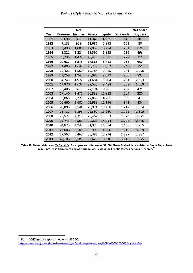
Portfolio Optimization & Monte Carlo Simulation
69
Year Revenue Net
Income Assets Equity Dividends Net Share Buyback
1991 6,695 860 11,349 4,835 148 109
1992 7,133 959 11,681 5,892 161 80
1993 7,408 1,083 12,035 6,274 201 620
1994 8,321 1,224 13,592 6,885 216 496
1995 9,795 1,427 15,415 7,861 227 315
1996 10,687 1,573 17,386 8,718 232 600
1997 11,409 1,642 18,242 8,852 248 755
1998 12,421 1,550 19,784 9,465 241 1,090
1999 13,259 1,948 20,983 9,639 265 892
2000 14,243 1,977 21,684 9,204 281 2,023
2001 14,870 1,637 22,535 9,488 288 1,068
2002 15,406 893 24,194 10,281 297 475
2003 17,140 1,471 25,838 11,982 504 220
2004 19,065 2,279 27,838 14,201 695 41
2005 20,460 2,602 29,989 15,146 842 434
2006 20,895 3,544 28,974 15,458 1,217 1,984
2007 22,787 2,395 29,392 15,280 1,766 2,805
2008 23,522 4,313 28,462 13,383 1,823 3,371
2009 22,745 4,551 30,225 14,034 2,236 2,465
2010 24,075 4,946 31,975 14,634 2,408 2,235
2011 27,006 5,503 32,990 14,390 2,610 3,029
2012 27,567 5,465 35,386 15,294 2,897 2,287
2013 28,106 5,586 36,626 16,010 3,115 1,545
Table 18: Financial data for McDonald’s. Fiscal year ends December 31. Net Share Buyback is calculated as Share Repurchase minus proceeds from exercising of stock options; excess tax benefit of stock options is ignored.
12
12
Form 10-K annual reports filed with US SEC: http://www.sec.gov/cgi-bin/browse-edgar?action=getcompany&CIK=0000063908&type=10-K
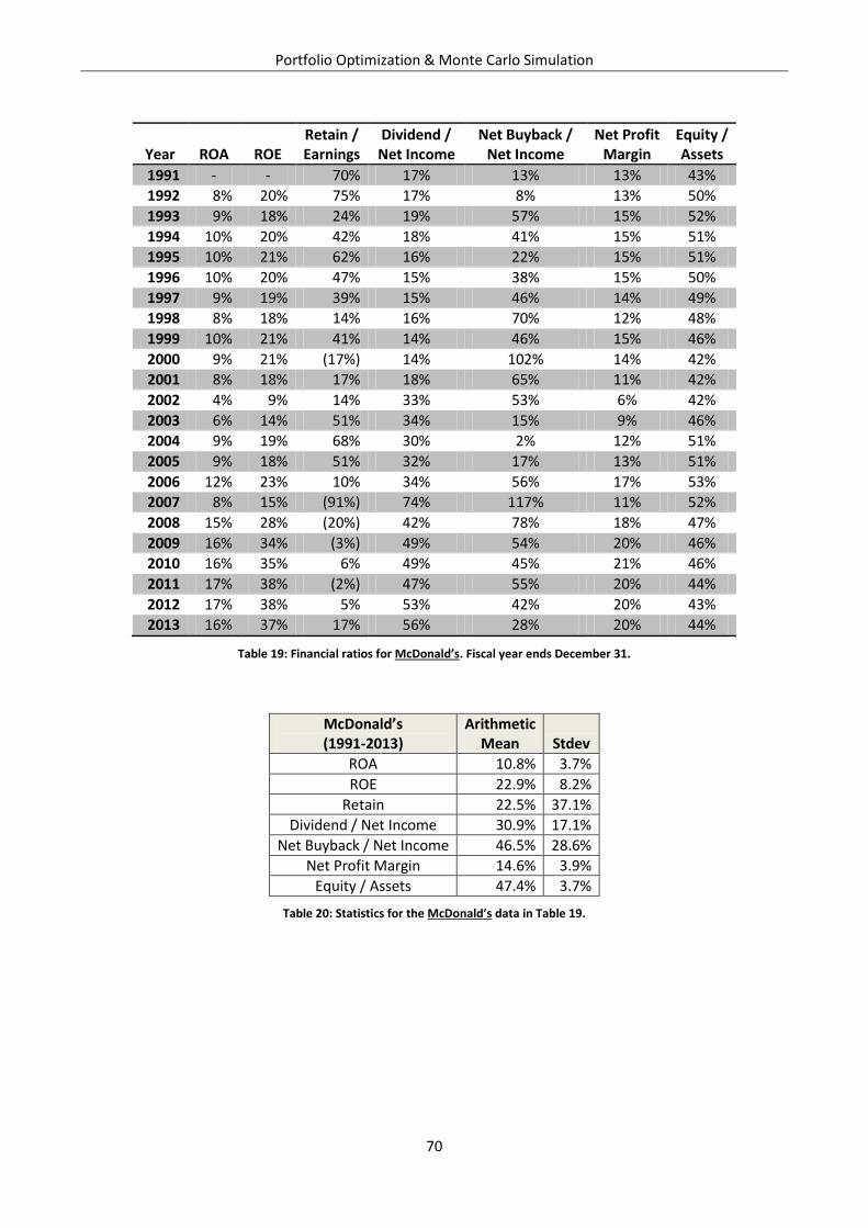
Portfolio Optimization & Monte Carlo Simulation
70
Year ROA ROE Retain / Earnings
Dividend / Net Income
Net Buyback / Net Income
Net Profit Margin
Equity / Assets
1991 - - 70% 17% 13% 13% 43%
1992 8% 20% 75% 17% 8% 13% 50%
1993 9% 18% 24% 19% 57% 15% 52%
1994 10% 20% 42% 18% 41% 15% 51%
1995 10% 21% 62% 16% 22% 15% 51%
1996 10% 20% 47% 15% 38% 15% 50%
1997 9% 19% 39% 15% 46% 14% 49%
1998 8% 18% 14% 16% 70% 12% 48%
1999 10% 21% 41% 14% 46% 15% 46%
2000 9% 21% (17%) 14% 102% 14% 42%
2001 8% 18% 17% 18% 65% 11% 42%
2002 4% 9% 14% 33% 53% 6% 42%
2003 6% 14% 51% 34% 15% 9% 46%
2004 9% 19% 68% 30% 2% 12% 51%
2005 9% 18% 51% 32% 17% 13% 51%
2006 12% 23% 10% 34% 56% 17% 53%
2007 8% 15% (91%) 74% 117% 11% 52%
2008 15% 28% (20%) 42% 78% 18% 47%
2009 16% 34% (3%) 49% 54% 20% 46%
2010 16% 35% 6% 49% 45% 21% 46%
2011 17% 38% (2%) 47% 55% 20% 44%
2012 17% 38% 5% 53% 42% 20% 43%
2013 16% 37% 17% 56% 28% 20% 44%
Table 19: Financial ratios for McDonald’s. Fiscal year ends December 31.
McDonald’s (1991-2013)
Arithmetic Mean Stdev
ROA 10.8% 3.7%
ROE 22.9% 8.2%
Retain 22.5% 37.1%
Dividend / Net Income 30.9% 17.1%
Net Buyback / Net Income 46.5% 28.6%
Net Profit Margin 14.6% 3.9%
Equity / Assets 47.4% 3.7%
Table 20: Statistics for the McDonald’s data in Table 19.
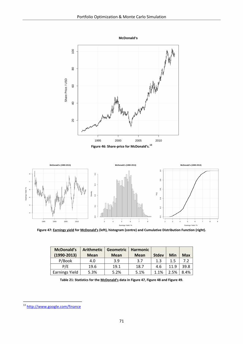
Portfolio Optimization & Monte Carlo Simulation
71
Figure 46: Share-price for McDonald’s.
13
Figure 47: Earnings yield for McDonald’s (left), histogram (centre) and Cumulative Distribution Function (right).
McDonald’s (1990-2013)
Arithmetic Mean
Geometric Mean
Harmonic Mean Stdev Min Max
P/Book 4.0 3.9 3.7 1.3 1.5 7.2
P/E 19.6 19.1 18.7 4.6 11.9 39.8
Earnings Yield 5.3% 5.2% 5.1% 1.1% 2.5% 8.4%
Table 21: Statistics for the McDonald’s data in Figure 47, Figure 48 and Figure 49.
13
http://www.google.com/finance
1995 2000 2005 2010
20
40
60
80
10
0
McDonald's
Sh
are
Price
/ U
SD
1995 2000 2005 2010
34
56
78
McDonald's (1990-2013)
Ea
rnin
gs Y
ield
/ %
McDonald's (1990-2013)
Earnings Yield / %
De
nsity
3 4 5 6 7 8
0.0
0.1
0.2
0.3
0.4
2 3 4 5 6 7 8 9
0.0
0.2
0.4
0.6
0.8
1.0
McDonald's (1990-2013)
Earnings Yield / %
F(x
)
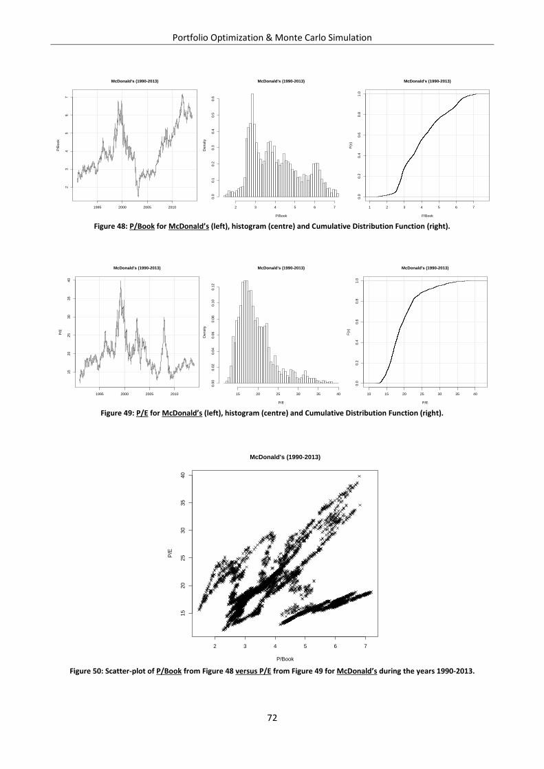
Portfolio Optimization & Monte Carlo Simulation
72
Figure 48: P/Book for McDonald’s (left), histogram (centre) and Cumulative Distribution Function (right).
Figure 49: P/E for McDonald’s (left), histogram (centre) and Cumulative Distribution Function (right).
Figure 50: Scatter-plot of P/Book from Figure 48 versus P/E from Figure 49 for McDonald’s during the years 1990-2013.
1995 2000 2005 2010
23
45
67
McDonald's (1990-2013)
P/B
oo
k
McDonald's (1990-2013)
P/Book
De
nsity
2 3 4 5 6 7
0.0
0.1
0.2
0.3
0.4
0.5
0.6
1 2 3 4 5 6 7
0.0
0.2
0.4
0.6
0.8
1.0
McDonald's (1990-2013)
P/Book
F(x
)
1995 2000 2005 2010
15
20
25
30
35
40
McDonald's (1990-2013)
P/E
McDonald's (1990-2013)
P/E
De
nsity
15 20 25 30 35 40
0.0
00
.02
0.0
40
.06
0.0
80
.10
0.1
2
10 15 20 25 30 35 40
0.0
0.2
0.4
0.6
0.8
1.0
McDonald's (1990-2013)
P/E
F(x
)
2 3 4 5 6 7
15
20
25
30
35
40
McDonald's (1990-2013)
P/Book
P/E
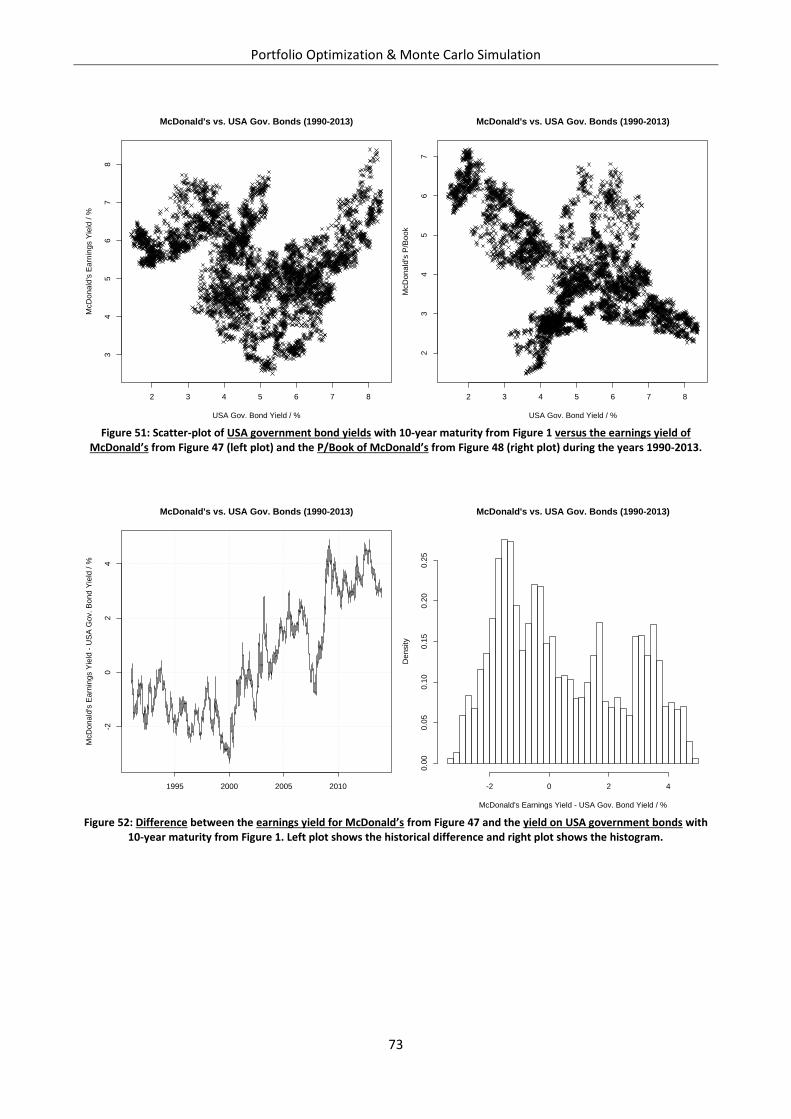
Portfolio Optimization & Monte Carlo Simulation
73
Figure 51: Scatter-plot of USA government bond yields with 10-year maturity from Figure 1 versus the earnings yield of
McDonald’s from Figure 47 (left plot) and the P/Book of McDonald’s from Figure 48 (right plot) during the years 1990-2013.
Figure 52: Difference between the earnings yield for McDonald’s from Figure 47 and the yield on USA government bonds with
10-year maturity from Figure 1. Left plot shows the historical difference and right plot shows the histogram.
2 3 4 5 6 7 8
34
56
78
McDonald's vs. USA Gov. Bonds (1990-2013)
USA Gov. Bond Yield / %
McD
on
ald
's E
arn
ings Y
ield
/ %
2 3 4 5 6 7 8
23
45
67
McDonald's vs. USA Gov. Bonds (1990-2013)
USA Gov. Bond Yield / %
McD
on
ald
's P
/Book
1995 2000 2005 2010
-20
24
McDonald's vs. USA Gov. Bonds (1990-2013)
McD
onald
's E
arn
ings Y
ield
- U
SA
Gov. B
ond Y
ield
/ %
McDonald's vs. USA Gov. Bonds (1990-2013)
McDonald's Earnings Yield - USA Gov. Bond Yield / %
Density
-2 0 2 4
0.0
00.0
50.1
00.1
50.2
00.2
5
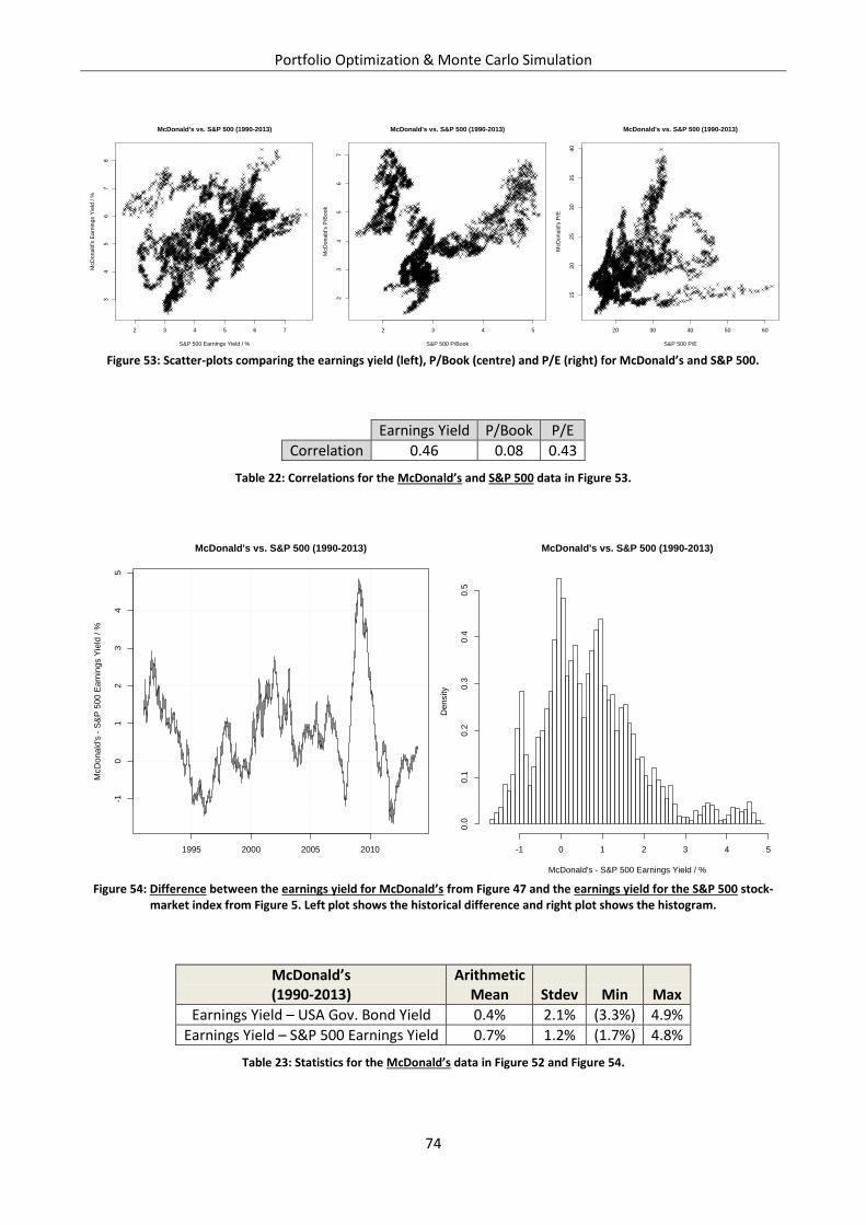
Portfolio Optimization & Monte Carlo Simulation
74
Figure 53: Scatter-plots comparing the earnings yield (left), P/Book (centre) and P/E (right) for McDonald’s and S&P 500.
Earnings Yield P/Book P/E
Correlation 0.46 0.08 0.43
Table 22: Correlations for the McDonald’s and S&P 500 data in Figure 53.
Figure 54: Difference between the earnings yield for McDonald’s from Figure 47 and the earnings yield for the S&P 500 stock-
market index from Figure 5. Left plot shows the historical difference and right plot shows the histogram.
McDonald’s (1990-2013)
Arithmetic Mean Stdev Min Max
Earnings Yield – USA Gov. Bond Yield 0.4% 2.1% (3.3%) 4.9%
Earnings Yield – S&P 500 Earnings Yield 0.7% 1.2% (1.7%) 4.8%
Table 23: Statistics for the McDonald’s data in Figure 52 and Figure 54.
2 3 4 5 6 7
34
56
78
McDonald's vs. S&P 500 (1990-2013)
S&P 500 Earnings Yield / %
McD
on
ald
's E
arn
ing
s Y
ield
/ %
2 3 4 5
23
45
67
McDonald's vs. S&P 500 (1990-2013)
S&P 500 P/Book
McD
on
ald
's P
/Bo
ok
20 30 40 50 60
15
20
25
30
35
40
McDonald's vs. S&P 500 (1990-2013)
S&P 500 P/E
McD
on
ald
's P
/E
1995 2000 2005 2010
-10
12
34
5
McDonald's vs. S&P 500 (1990-2013)
McD
onald
's -
S&
P 5
00 E
arn
ings Y
ield
/ %
McDonald's vs. S&P 500 (1990-2013)
McDonald's - S&P 500 Earnings Yield / %
Density
-1 0 1 2 3 4 5
0.0
0.1
0.2
0.3
0.4
0.5
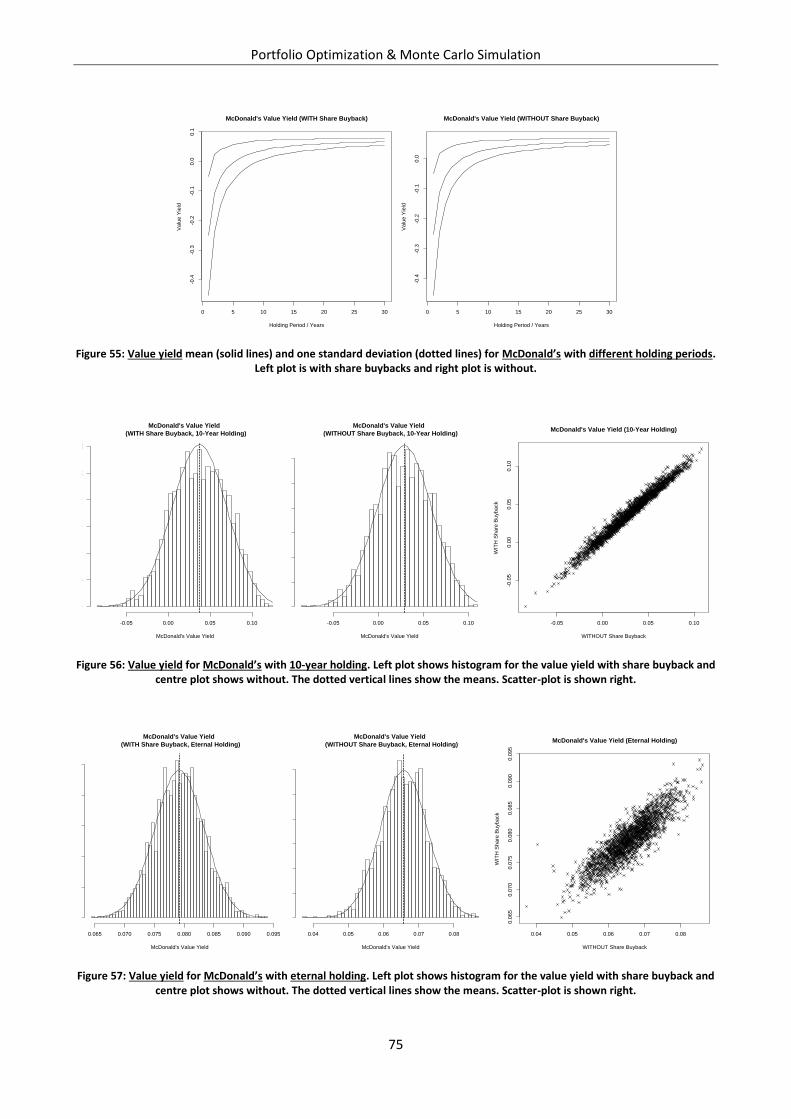
Portfolio Optimization & Monte Carlo Simulation
75
Figure 55: Value yield mean (solid lines) and one standard deviation (dotted lines) for McDonald’s with different holding periods. Left plot is with share buybacks and right plot is without.
Figure 56: Value yield for McDonald’s with 10-year holding. Left plot shows histogram for the value yield with share buyback and centre plot shows without. The dotted vertical lines show the means. Scatter-plot is shown right.
Figure 57: Value yield for McDonald’s with eternal holding. Left plot shows histogram for the value yield with share buyback and centre plot shows without. The dotted vertical lines show the means. Scatter-plot is shown right.
0 5 10 15 20 25 30
-0.4
-0.3
-0.2
-0.1
0.0
0.1
McDonald's Value Yield (WITH Share Buyback)
Holding Period / Years
Valu
e Y
ield
0 5 10 15 20 25 30
-0.4
-0.3
-0.2
-0.1
0.0
McDonald's Value Yield (WITHOUT Share Buyback)
Holding Period / Years
Valu
e Y
ield
McDonald's Value Yield
(WITH Share Buyback, 10-Year Holding)
McDonald's Value Yield
Density
-0.05 0.00 0.05 0.10
02
46
810
12
McDonald's Value Yield
(WITHOUT Share Buyback, 10-Year Holding)
McDonald's Value Yield
Density
-0.05 0.00 0.05 0.10
02
46
810
12
-0.05 0.00 0.05 0.10
-0.0
50.0
00.0
50.1
0
McDonald's Value Yield (10-Year Holding)
WITHOUT Share Buyback
WIT
H S
hare
Buyback
McDonald's Value Yield
(WITH Share Buyback, Eternal Holding)
McDonald's Value Yield
Density
0.065 0.070 0.075 0.080 0.085 0.090 0.095
020
40
60
80
100
McDonald's Value Yield
(WITHOUT Share Buyback, Eternal Holding)
McDonald's Value Yield
Density
0.04 0.05 0.06 0.07 0.08
010
20
30
40
50
60
0.04 0.05 0.06 0.07 0.08
0.0
65
0.0
70
0.0
75
0.0
80
0.0
85
0.0
90
0.0
95
McDonald's Value Yield (Eternal Holding)
WITHOUT Share Buyback
WIT
H S
hare
Buyback
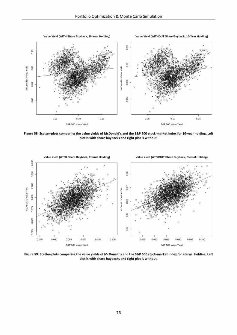
Portfolio Optimization & Monte Carlo Simulation
76
Figure 58: Scatter-plots comparing the value yields of McDonald’s and the S&P 500 stock-market index for 10-year holding. Left plot is with share buybacks and right plot is without.
Figure 59: Scatter-plots comparing the value yields of McDonald’s and the S&P 500 stock-market index for eternal holding. Left plot is with share buybacks and right plot is without.
0.05 0.10 0.15
-0.0
50
.00
0.0
50
.10
Value Yield (WITH Share Buyback, 10-Year Holding)
S&P 500 Value Yield
McD
on
ald
's V
alu
e Y
ield
0.05 0.10 0.15
-0.0
50
.00
0.0
50
.10
Value Yield (WITHOUT Share Buyback, 10-Year Holding)
S&P 500 Value Yield
McD
on
ald
's V
alu
e Y
ield
0.075 0.080 0.085 0.090 0.095 0.100
0.0
65
0.0
70
0.0
75
0.0
80
0.0
85
0.0
90
0.0
95
Value Yield (WITH Share Buyback, Eternal Holding)
S&P 500 Value Yield
McD
on
ald
's V
alu
e Y
ield
0.075 0.080 0.085 0.090 0.095 0.100
0.0
40
.05
0.0
60
.07
0.0
8
Value Yield (WITHOUT Share Buyback, Eternal Holding)
S&P 500 Value Yield
McD
on
ald
's V
alu
e Y
ield
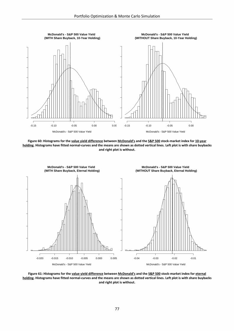
Portfolio Optimization & Monte Carlo Simulation
77
Figure 60: Histograms for the value yield difference between McDonald’s and the S&P 500 stock-market index for 10-year holding. Histograms have fitted normal-curves and the means are shown as dotted vertical lines. Left plot is with share buybacks
and right plot is without.
Figure 61: Histograms for the value yield difference between McDonald’s and the S&P 500 stock-market index for eternal holding. Histograms have fitted normal-curves and the means are shown as dotted vertical lines. Left plot is with share buybacks
and right plot is without.
McDonald's - S&P 500 Value Yield
(WITH Share Buyback, 10-Year Holding)
McDonald's - S&P 500 Value Yield
Density
-0.15 -0.10 -0.05 0.00 0.05
02
46
810
12
14
McDonald's - S&P 500 Value Yield
(WITHOUT Share Buyback, 10-Year Holding)
McDonald's - S&P 500 Value Yield
Density
-0.15 -0.10 -0.05 0.00
02
46
810
12
14
McDonald's - S&P 500 Value Yield
(WITH Share Buyback, Eternal Holding)
McDonald's - S&P 500 Value Yield
De
nsity
-0.020 -0.015 -0.010 -0.005 0.000 0.005
02
04
06
08
01
00
12
0
McDonald's - S&P 500 Value Yield
(WITHOUT Share Buyback, Eternal Holding)
McDonald's - S&P 500 Value Yield
Density
-0.04 -0.03 -0.02 -0.01
010
20
30
40
50
60
70
Portfolio Optimization & Monte Carlo Simulation
78
Figures & Tables
Company Comparison
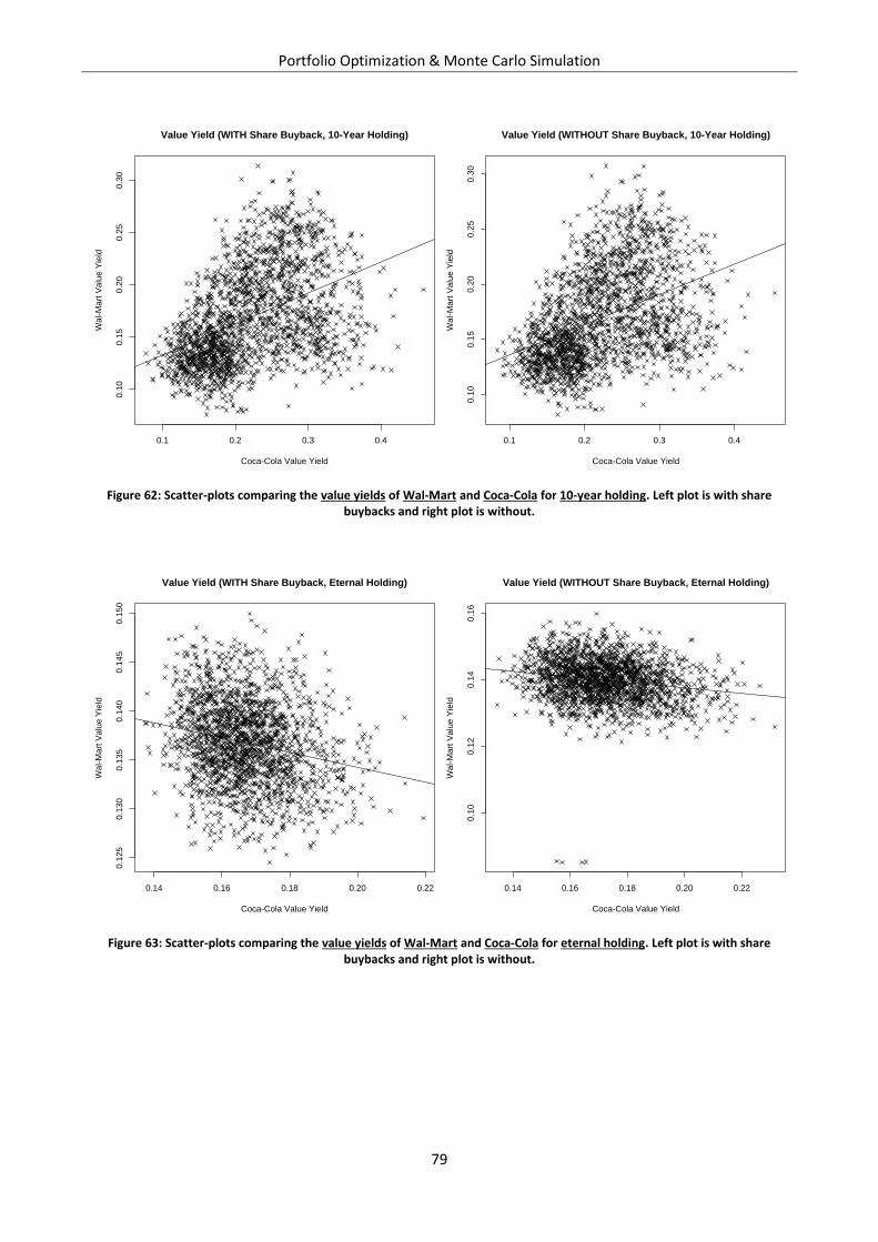
Portfolio Optimization & Monte Carlo Simulation
79
Figure 62: Scatter-plots comparing the value yields of Wal-Mart and Coca-Cola for 10-year holding. Left plot is with share buybacks and right plot is without.
Figure 63: Scatter-plots comparing the value yields of Wal-Mart and Coca-Cola for eternal holding. Left plot is with share buybacks and right plot is without.
0.1 0.2 0.3 0.4
0.1
00.1
50.2
00.2
50.3
0
Value Yield (WITH Share Buyback, 10-Year Holding)
Coca-Cola Value Yield
Wal-M
art
Va
lue
Yie
ld
0.1 0.2 0.3 0.4
0.1
00
.15
0.2
00
.25
0.3
0
Value Yield (WITHOUT Share Buyback, 10-Year Holding)
Coca-Cola Value Yield
Wal-M
art
Va
lue
Yie
ld
0.14 0.16 0.18 0.20 0.22
0.1
25
0.1
30
0.1
35
0.1
40
0.1
45
0.1
50
Value Yield (WITH Share Buyback, Eternal Holding)
Coca-Cola Value Yield
Wal-M
art
Valu
e Y
ield
0.14 0.16 0.18 0.20 0.22
0.1
00.1
20.1
40.1
6
Value Yield (WITHOUT Share Buyback, Eternal Holding)
Coca-Cola Value Yield
Wal-M
art
Valu
e Y
ield
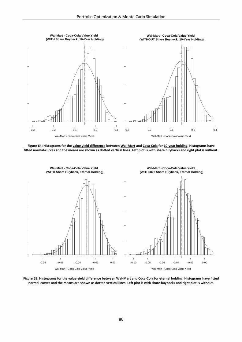
Portfolio Optimization & Monte Carlo Simulation
80
Figure 64: Histograms for the value yield difference between Wal-Mart and Coca-Cola for 10-year holding. Histograms have fitted normal-curves and the means are shown as dotted vertical lines. Left plot is with share buybacks and right plot is without.
Figure 65: Histograms for the value yield difference between Wal-Mart and Coca-Cola for eternal holding. Histograms have fitted normal-curves and the means are shown as dotted vertical lines. Left plot is with share buybacks and right plot is without.
Wal-Mart - Coca-Cola Value Yield
(WITH Share Buyback, 10-Year Holding)
Wal-Mart - Coca-Cola Value Yield
Density
-0.3 -0.2 -0.1 0.0 0.1
02
46
8
Wal-Mart - Coca-Cola Value Yield
(WITHOUT Share Buyback, 10-Year Holding)
Wal-Mart - Coca-Cola Value Yield
Density
-0.3 -0.2 -0.1 0.0 0.1
02
46
8
Wal-Mart - Coca-Cola Value Yield
(WITH Share Buyback, Eternal Holding)
Wal-Mart - Coca-Cola Value Yield
Density
-0.08 -0.06 -0.04 -0.02 0.00
05
10
15
20
25
30
Wal-Mart - Coca-Cola Value Yield
(WITHOUT Share Buyback, Eternal Holding)
Wal-Mart - Coca-Cola Value Yield
Density
-0.10 -0.08 -0.06 -0.04 -0.02 0.00
05
10
15
20
25
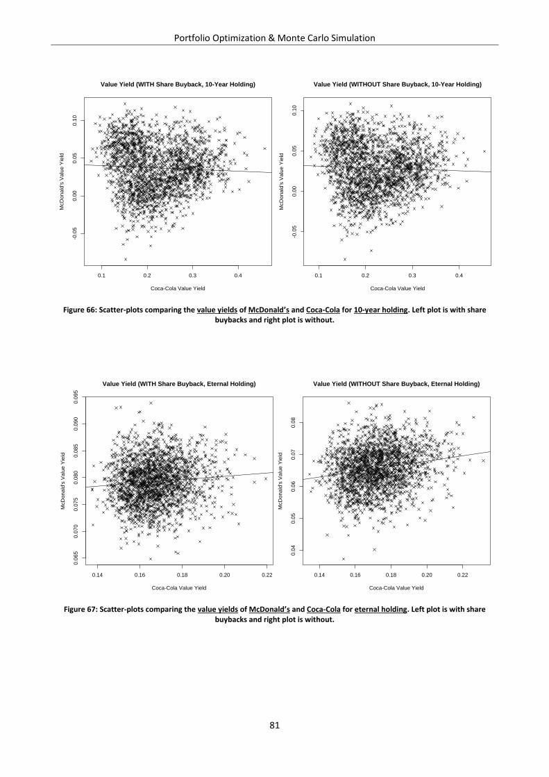
Portfolio Optimization & Monte Carlo Simulation
81
Figure 66: Scatter-plots comparing the value yields of McDonald’s and Coca-Cola for 10-year holding. Left plot is with share buybacks and right plot is without.
Figure 67: Scatter-plots comparing the value yields of McDonald’s and Coca-Cola for eternal holding. Left plot is with share buybacks and right plot is without.
0.1 0.2 0.3 0.4
-0.0
50.0
00.0
50.1
0
Value Yield (WITH Share Buyback, 10-Year Holding)
Coca-Cola Value Yield
McD
onald
's V
alu
e Y
ield
0.1 0.2 0.3 0.4
-0.0
50
.00
0.0
50.1
0
Value Yield (WITHOUT Share Buyback, 10-Year Holding)
Coca-Cola Value Yield
McD
onald
's V
alu
e Y
ield
0.14 0.16 0.18 0.20 0.22
0.0
65
0.0
70
0.0
75
0.0
80
0.0
85
0.0
90
0.0
95
Value Yield (WITH Share Buyback, Eternal Holding)
Coca-Cola Value Yield
McD
onald
's V
alu
e Y
ield
0.14 0.16 0.18 0.20 0.22
0.0
40.0
50.0
60.0
70.0
8
Value Yield (WITHOUT Share Buyback, Eternal Holding)
Coca-Cola Value Yield
McD
onald
's V
alu
e Y
ield
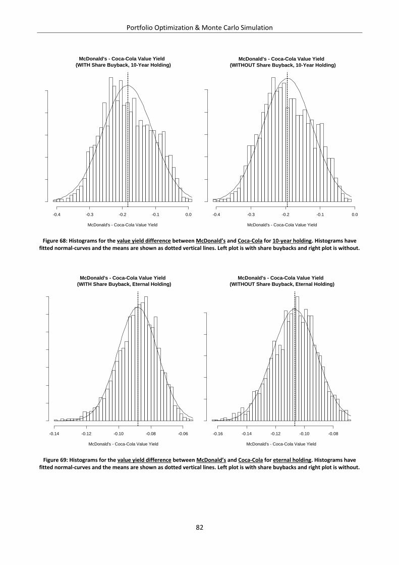
Portfolio Optimization & Monte Carlo Simulation
82
Figure 68: Histograms for the value yield difference between McDonald’s and Coca-Cola for 10-year holding. Histograms have fitted normal-curves and the means are shown as dotted vertical lines. Left plot is with share buybacks and right plot is without.
Figure 69: Histograms for the value yield difference between McDonald’s and Coca-Cola for eternal holding. Histograms have fitted normal-curves and the means are shown as dotted vertical lines. Left plot is with share buybacks and right plot is without.
McDonald's - Coca-Cola Value Yield
(WITH Share Buyback, 10-Year Holding)
McDonald's - Coca-Cola Value Yield
Density
-0.4 -0.3 -0.2 -0.1 0.0
01
23
45
McDonald's - Coca-Cola Value Yield
(WITHOUT Share Buyback, 10-Year Holding)
McDonald's - Coca-Cola Value Yield
Density
-0.4 -0.3 -0.2 -0.1 0.0
01
23
45
McDonald's - Coca-Cola Value Yield
(WITH Share Buyback, Eternal Holding)
McDonald's - Coca-Cola Value Yield
Density
-0.14 -0.12 -0.10 -0.08 -0.06
05
10
15
20
25
30
35
McDonald's - Coca-Cola Value Yield
(WITHOUT Share Buyback, Eternal Holding)
McDonald's - Coca-Cola Value Yield
Density
-0.16 -0.14 -0.12 -0.10 -0.08
05
10
15
20
25
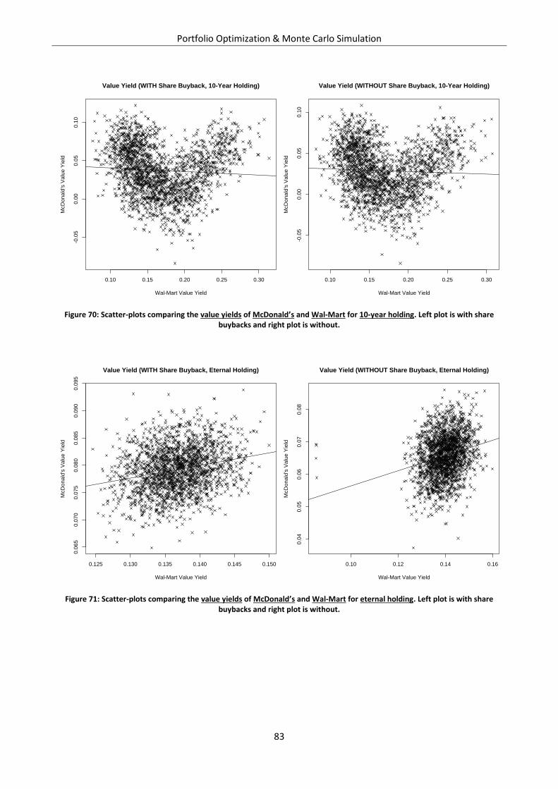
Portfolio Optimization & Monte Carlo Simulation
83
Figure 70: Scatter-plots comparing the value yields of McDonald’s and Wal-Mart for 10-year holding. Left plot is with share buybacks and right plot is without.
Figure 71: Scatter-plots comparing the value yields of McDonald’s and Wal-Mart for eternal holding. Left plot is with share buybacks and right plot is without.
0.10 0.15 0.20 0.25 0.30
-0.0
50.0
00.0
50.1
0
Value Yield (WITH Share Buyback, 10-Year Holding)
Wal-Mart Value Yield
McD
onald
's V
alu
e Y
ield
0.10 0.15 0.20 0.25 0.30
-0.0
50
.00
0.0
50.1
0
Value Yield (WITHOUT Share Buyback, 10-Year Holding)
Wal-Mart Value Yield
McD
onald
's V
alu
e Y
ield
0.125 0.130 0.135 0.140 0.145 0.150
0.0
65
0.0
70
0.0
75
0.0
80
0.0
85
0.0
90
0.0
95
Value Yield (WITH Share Buyback, Eternal Holding)
Wal-Mart Value Yield
McD
onald
's V
alu
e Y
ield
0.10 0.12 0.14 0.16
0.0
40.0
50.0
60.0
70.0
8
Value Yield (WITHOUT Share Buyback, Eternal Holding)
Wal-Mart Value Yield
McD
onald
's V
alu
e Y
ield
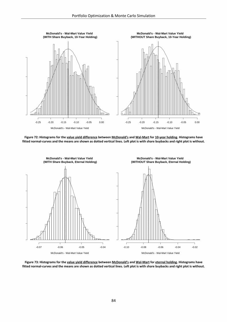
Portfolio Optimization & Monte Carlo Simulation
84
Figure 72: Histograms for the value yield difference between McDonald’s and Wal-Mart for 10-year holding. Histograms have fitted normal-curves and the means are shown as dotted vertical lines. Left plot is with share buybacks and right plot is without.
Figure 73: Histograms for the value yield difference between McDonald’s and Wal-Mart for eternal holding. Histograms have fitted normal-curves and the means are shown as dotted vertical lines. Left plot is with share buybacks and right plot is without.
McDonald's - Wal-Mart Value Yield
(WITH Share Buyback, 10-Year Holding)
McDonald's - Wal-Mart Value Yield
Density
-0.25 -0.20 -0.15 -0.10 -0.05 0.00
02
46
McDonald's - Wal-Mart Value Yield
(WITHOUT Share Buyback, 10-Year Holding)
McDonald's - Wal-Mart Value Yield
Density
-0.25 -0.20 -0.15 -0.10 -0.05 0.00
02
46
8
McDonald's - Wal-Mart Value Yield
(WITH Share Buyback, Eternal Holding)
McDonald's - Wal-Mart Value Yield
Density
-0.07 -0.06 -0.05 -0.04
020
40
60
80
McDonald's - Wal-Mart Value Yield
(WITHOUT Share Buyback, Eternal Holding)
McDonald's - Wal-Mart Value Yield
Density
-0.10 -0.08 -0.06 -0.04 -0.02
010
20
30
40
50
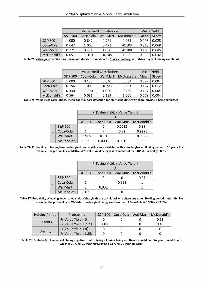
Portfolio Optimization & Monte Carlo Simulation
85
Value Yield Correlations Value Yield
S&P 500 Coca-Cola Wal-Mart McDonald’s Mean Stdev
S&P 500 1.000 0.647 0.771 0.051 0.095 0.028
Coca-Cola 0.647 1.000 0.471 -0.103 0.218 0.068
Wal-Mart 0.771 0.471 1.000 -0.108 0.166 0.045
McDonald’s 0.051 -0.103 -0.108 1.000 0.038 0.032 Table 24: Value yield correlations, mean and standard deviation for 10-year holding, with share buybacks being simulated.
Value Yield Correlations Value Yield
S&P 500 Coca-Cola Wal-Mart McDonald’s Mean Stdev
S&P 500 1.000 0.156 0.340 0.564 0.087 0.004
Coca-Cola 0.156 1.000 -0.223 0.031 0.167 0.012
Wal-Mart 0.340 -0.223 1.000 0.189 0.137 0.004
McDonald’s 0.564 0.031 0.189 1.000 0.079 0.004 Table 25: Value yield correlations, mean and standard deviation for eternal holding, with share buybacks being simulated.
Pr[Value YieldX < Value YieldY]
X
S&P 500 Coca-Cola Wal-Mart McDonald’s
Y
S&P 500 - 0 0.0035 0.88
Coca-Cola 1 - 0.82 0.9995
Wal-Mart 0.9965 0.18 - 0.9985
McDonald’s 0.12 0.0005 0.0015 -
Table 26: Probability of having lower value yield. Value yields are calculated with share buybacks. Holding period is 10 years. For example, the probability of McDonald’s value yield being less than that of the S&P 500 is 0.88 (or 88%).
Pr[Value YieldX < Value YieldY]
X
S&P 500 Coca-Cola Wal-Mart McDonald’s
Y
S&P 500 - 0 0 0.97
Coca-Cola 1 - 0.998 1
Wal-Mart 1 0.002 - 1
McDonald’s 0.03 0 0 -
Table 27: Probability of having lower value yield. Value yields are calculated with share buybacks. Holding period is eternity. For example, the probability of Wal-Mart’s value yield being less than that of Coca-Cola is 0.998 (or 99.8%).
Holding Period Probability S&P 500 Coca-Cola Wal-Mart McDonald’s
10 Years Pr[Value Yield < 0] 0 0 0 0.13
Pr[Value Yield < 2.7%] 0.001 0 0 0.40
Eternity Pr[Value Yield < 0] 0 0 0 0
Pr[Value Yield < 3.5%] 0 0 0 0
Table 28: Probability of value yield being negative (that is, being a loss) or being less than the yield on USA government bonds which is 2.7% for 10-year maturity and 3.5% for 30-year maturity.
Portfolio Optimization & Monte Carlo Simulation
86
Figures & Tables
Mean-Variance Portfolios
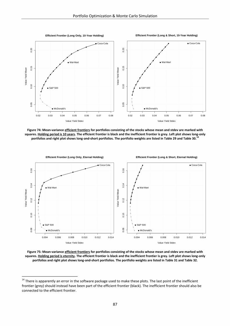
Portfolio Optimization & Monte Carlo Simulation
87
Figure 74: Mean-variance efficient frontiers for portfolios consisting of the stocks whose mean and stdev are marked with squares. Holding period is 10 years. The efficient frontier is black and the inefficient frontier is grey. Left plot shows long-only
portfolios and right plot shows long-and-short portfolios. The portfolio weights are listed in Table 29 and Table 30.14
Figure 75: Mean-variance efficient frontiers for portfolios consisting of the stocks whose mean and stdev are marked with squares. Holding period is eternity. The efficient frontier is black and the inefficient frontier is grey. Left plot shows long-only
portfolios and right plot shows long-and-short portfolios. The portfolio weights are listed in Table 31 and Table 32.
14
There is apparently an error in the software package used to make these plots. The last point of the inefficient frontier (grey) should instead have been part of the efficient frontier (black). The inefficient frontier should also be connected to the efficient frontier.
0.02 0.03 0.04 0.05 0.06 0.07 0.08
0.0
50.1
00.1
50.2
0
MV
| s
olv
eR
qu
ad
pro
gM
V | s
olv
eR
qu
ad
pro
g
Efficient Frontier (Long Only, 10-Year Holding)
Value Yield Stdev
Valu
e Y
ield
Mean
S&P 500
Coca-Cola
Wal-Mart
McDonald's
0.02 0.03 0.04 0.05 0.06 0.07 0.08
0.0
50.1
00.1
50.2
0
MV
| s
olv
eR
sh
ort
Exa
ct
MV
| s
olv
eR
sh
ort
Exa
ct
Efficient Frontier (Long & Short, 10-Year Holding)
Value Yield Stdev
Valu
e Y
ield
Mean
S&P 500
Coca-Cola
Wal-Mart
McDonald's
0.004 0.006 0.008 0.010 0.012 0.014
0.0
80.1
00.1
20.1
40.1
6
MV
| s
olv
eR
qu
ad
pro
gM
V | s
olv
eR
qu
ad
pro
g
Efficient Frontier (Long Only, Eternal Holding)
Value Yield Stdev
Valu
e Y
ield
Mean
S&P 500
Coca-Cola
Wal-Mart
McDonald's
0.004 0.006 0.008 0.010 0.012 0.014
0.0
80.1
00.1
20.1
40.1
6
MV
| s
olv
eR
sh
ort
Exa
ct
MV
| s
olv
eR
sh
ort
Exa
ct
Efficient Frontier (Long & Short, Eternal Holding)
Value Yield Stdev
Valu
e Y
ield
Mean
S&P 500
Coca-Cola
Wal-Mart
McDonald's
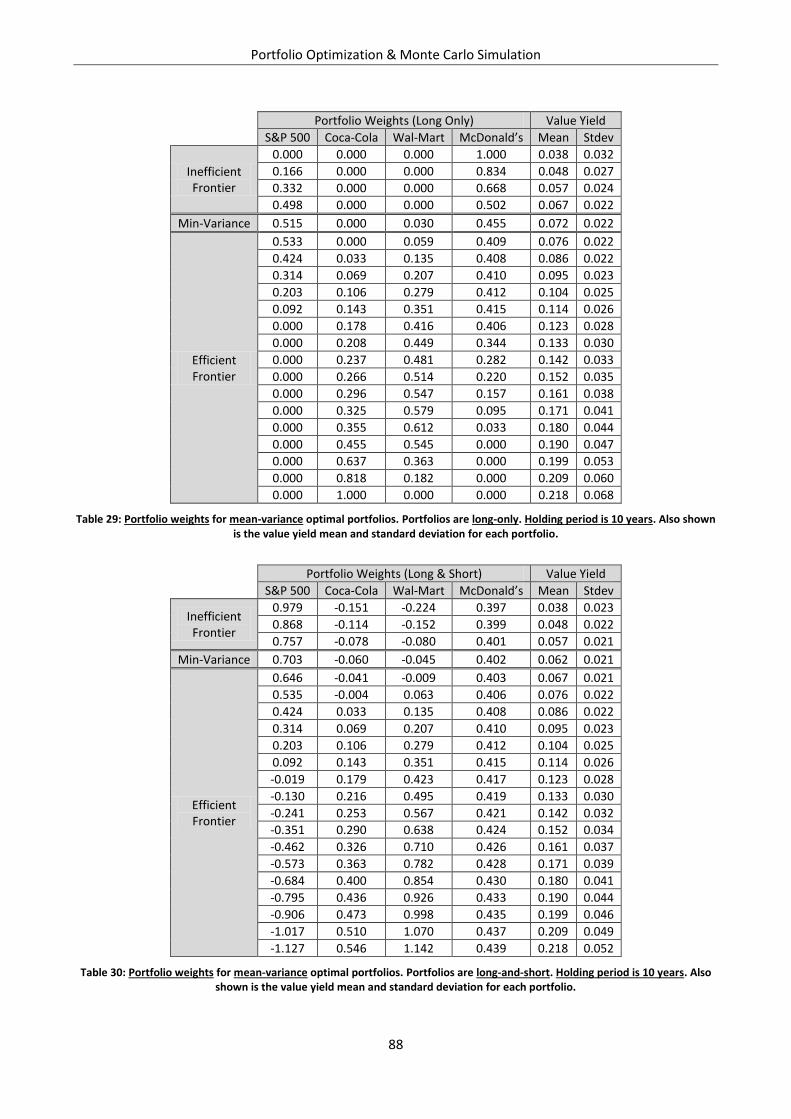
Portfolio Optimization & Monte Carlo Simulation
88
Portfolio Weights (Long Only) Value Yield
S&P 500 Coca-Cola Wal-Mart McDonald’s Mean Stdev
Inefficient Frontier
0.000 0.000 0.000 1.000 0.038 0.032
0.166 0.000 0.000 0.834 0.048 0.027
0.332 0.000 0.000 0.668 0.057 0.024
0.498 0.000 0.000 0.502 0.067 0.022
Min-Variance 0.515 0.000 0.030 0.455 0.072 0.022
Efficient Frontier
0.533 0.000 0.059 0.409 0.076 0.022
0.424 0.033 0.135 0.408 0.086 0.022
0.314 0.069 0.207 0.410 0.095 0.023
0.203 0.106 0.279 0.412 0.104 0.025
0.092 0.143 0.351 0.415 0.114 0.026
0.000 0.178 0.416 0.406 0.123 0.028
0.000 0.208 0.449 0.344 0.133 0.030
0.000 0.237 0.481 0.282 0.142 0.033
0.000 0.266 0.514 0.220 0.152 0.035
0.000 0.296 0.547 0.157 0.161 0.038
0.000 0.325 0.579 0.095 0.171 0.041
0.000 0.355 0.612 0.033 0.180 0.044
0.000 0.455 0.545 0.000 0.190 0.047
0.000 0.637 0.363 0.000 0.199 0.053
0.000 0.818 0.182 0.000 0.209 0.060
0.000 1.000 0.000 0.000 0.218 0.068
Table 29: Portfolio weights for mean-variance optimal portfolios. Portfolios are long-only. Holding period is 10 years. Also shown is the value yield mean and standard deviation for each portfolio.
Portfolio Weights (Long & Short) Value Yield
S&P 500 Coca-Cola Wal-Mart McDonald’s Mean Stdev
Inefficient Frontier
0.979 -0.151 -0.224 0.397 0.038 0.023
0.868 -0.114 -0.152 0.399 0.048 0.022
0.757 -0.078 -0.080 0.401 0.057 0.021
Min-Variance 0.703 -0.060 -0.045 0.402 0.062 0.021
Efficient Frontier
0.646 -0.041 -0.009 0.403 0.067 0.021
0.535 -0.004 0.063 0.406 0.076 0.022
0.424 0.033 0.135 0.408 0.086 0.022
0.314 0.069 0.207 0.410 0.095 0.023
0.203 0.106 0.279 0.412 0.104 0.025
0.092 0.143 0.351 0.415 0.114 0.026
-0.019 0.179 0.423 0.417 0.123 0.028
-0.130 0.216 0.495 0.419 0.133 0.030
-0.241 0.253 0.567 0.421 0.142 0.032
-0.351 0.290 0.638 0.424 0.152 0.034
-0.462 0.326 0.710 0.426 0.161 0.037
-0.573 0.363 0.782 0.428 0.171 0.039
-0.684 0.400 0.854 0.430 0.180 0.041
-0.795 0.436 0.926 0.433 0.190 0.044
-0.906 0.473 0.998 0.435 0.199 0.046
-1.017 0.510 1.070 0.437 0.209 0.049
-1.127 0.546 1.142 0.439 0.218 0.052
Table 30: Portfolio weights for mean-variance optimal portfolios. Portfolios are long-and-short. Holding period is 10 years. Also shown is the value yield mean and standard deviation for each portfolio.
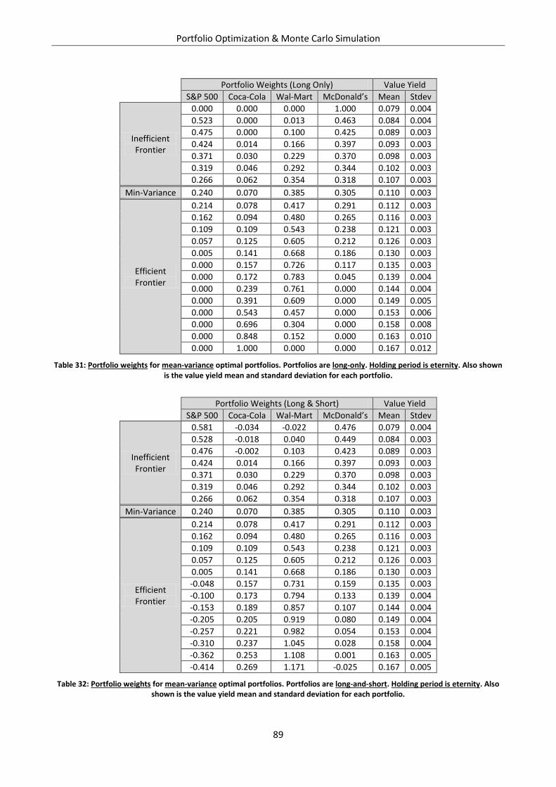
Portfolio Optimization & Monte Carlo Simulation
89
Portfolio Weights (Long Only) Value Yield
S&P 500 Coca-Cola Wal-Mart McDonald’s Mean Stdev
Inefficient Frontier
0.000 0.000 0.000 1.000 0.079 0.004
0.523 0.000 0.013 0.463 0.084 0.004
0.475 0.000 0.100 0.425 0.089 0.003
0.424 0.014 0.166 0.397 0.093 0.003
0.371 0.030 0.229 0.370 0.098 0.003
0.319 0.046 0.292 0.344 0.102 0.003
0.266 0.062 0.354 0.318 0.107 0.003
Min-Variance 0.240 0.070 0.385 0.305 0.110 0.003
Efficient Frontier
0.214 0.078 0.417 0.291 0.112 0.003
0.162 0.094 0.480 0.265 0.116 0.003
0.109 0.109 0.543 0.238 0.121 0.003
0.057 0.125 0.605 0.212 0.126 0.003
0.005 0.141 0.668 0.186 0.130 0.003
0.000 0.157 0.726 0.117 0.135 0.003
0.000 0.172 0.783 0.045 0.139 0.004
0.000 0.239 0.761 0.000 0.144 0.004
0.000 0.391 0.609 0.000 0.149 0.005
0.000 0.543 0.457 0.000 0.153 0.006
0.000 0.696 0.304 0.000 0.158 0.008
0.000 0.848 0.152 0.000 0.163 0.010
0.000 1.000 0.000 0.000 0.167 0.012
Table 31: Portfolio weights for mean-variance optimal portfolios. Portfolios are long-only. Holding period is eternity. Also shown is the value yield mean and standard deviation for each portfolio.
Portfolio Weights (Long & Short) Value Yield
S&P 500 Coca-Cola Wal-Mart McDonald’s Mean Stdev
Inefficient Frontier
0.581 -0.034 -0.022 0.476 0.079 0.004
0.528 -0.018 0.040 0.449 0.084 0.003
0.476 -0.002 0.103 0.423 0.089 0.003
0.424 0.014 0.166 0.397 0.093 0.003
0.371 0.030 0.229 0.370 0.098 0.003
0.319 0.046 0.292 0.344 0.102 0.003
0.266 0.062 0.354 0.318 0.107 0.003
Min-Variance 0.240 0.070 0.385 0.305 0.110 0.003
Efficient Frontier
0.214 0.078 0.417 0.291 0.112 0.003
0.162 0.094 0.480 0.265 0.116 0.003
0.109 0.109 0.543 0.238 0.121 0.003
0.057 0.125 0.605 0.212 0.126 0.003
0.005 0.141 0.668 0.186 0.130 0.003
-0.048 0.157 0.731 0.159 0.135 0.003
-0.100 0.173 0.794 0.133 0.139 0.004
-0.153 0.189 0.857 0.107 0.144 0.004
-0.205 0.205 0.919 0.080 0.149 0.004
-0.257 0.221 0.982 0.054 0.153 0.004
-0.310 0.237 1.045 0.028 0.158 0.004
-0.362 0.253 1.108 0.001 0.163 0.005
-0.414 0.269 1.171 -0.025 0.167 0.005
Table 32: Portfolio weights for mean-variance optimal portfolios. Portfolios are long-and-short. Holding period is eternity. Also shown is the value yield mean and standard deviation for each portfolio.
Portfolio Optimization & Monte Carlo Simulation
90
Figures & Tables
Kelly Portfolios
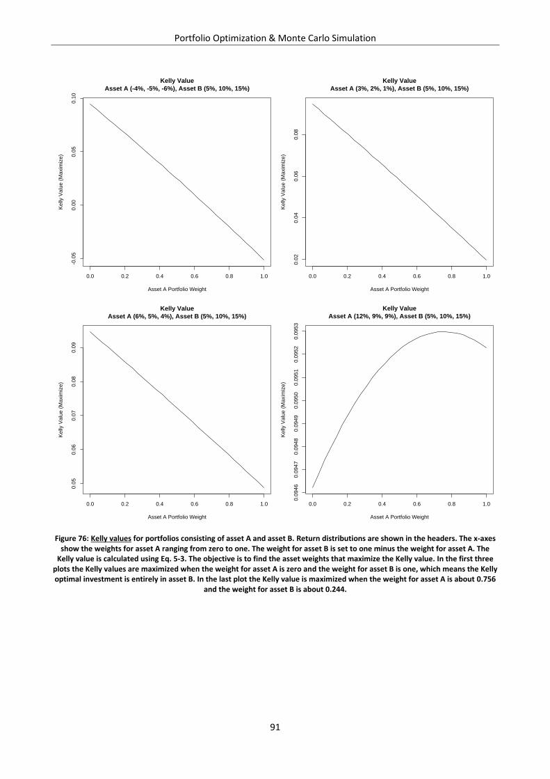
Portfolio Optimization & Monte Carlo Simulation
91
Figure 76: Kelly values for portfolios consisting of asset A and asset B. Return distributions are shown in the headers. The x-axes show the weights for asset A ranging from zero to one. The weight for asset B is set to one minus the weight for asset A. The
Kelly value is calculated using Eq. 5-3. The objective is to find the asset weights that maximize the Kelly value. In the first three plots the Kelly values are maximized when the weight for asset A is zero and the weight for asset B is one, which means the Kelly optimal investment is entirely in asset B. In the last plot the Kelly value is maximized when the weight for asset A is about 0.756
and the weight for asset B is about 0.244.
0.0 0.2 0.4 0.6 0.8 1.0
-0.0
50.0
00.0
50.1
0
Kelly Value
Asset A (-4%, -5%, -6%), Asset B (5%, 10%, 15%)
Asset A Portfolio Weight
Kelly
Va
lue
(M
axim
ize)
0.0 0.2 0.4 0.6 0.8 1.0
0.0
20
.04
0.0
60.0
8
Kelly Value
Asset A (3%, 2%, 1%), Asset B (5%, 10%, 15%)
Asset A Portfolio Weight
Kelly
Valu
e (
Maxim
ize)
0.0 0.2 0.4 0.6 0.8 1.0
0.0
50.0
60.0
70.0
80.0
9
Kelly Value
Asset A (6%, 5%, 4%), Asset B (5%, 10%, 15%)
Asset A Portfolio Weight
Kelly
Valu
e (
Maxim
ize)
0.0 0.2 0.4 0.6 0.8 1.0
0.0
94
60
.09
47
0.0
94
80
.09
49
0.0
95
00
.09
51
0.0
95
20
.09
53
Kelly Value
Asset A (12%, 9%, 9%), Asset B (5%, 10%, 15%)
Asset A Portfolio Weight
Ke
lly V
alu
e (
Ma
xim
ize
)
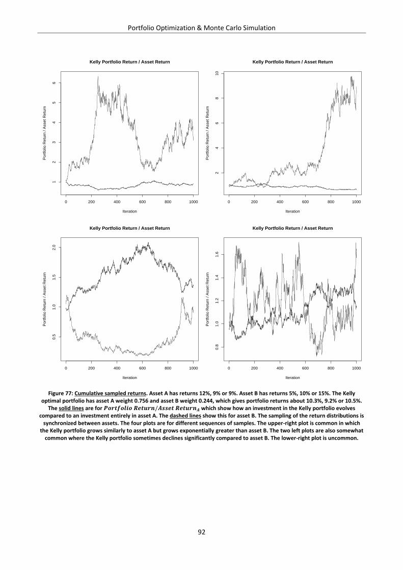
Portfolio Optimization & Monte Carlo Simulation
92
Figure 77: Cumulative sampled returns. Asset A has returns 12%, 9% or 9%. Asset B has returns 5%, 10% or 15%. The Kelly optimal portfolio has asset A weight 0.756 and asset B weight 0.244, which gives portfolio returns about 10.3%, 9.2% or 10.5%.
The solid lines are for which show how an investment in the Kelly portfolio evolves compared to an investment entirely in asset A. The dashed lines show this for asset B. The sampling of the return distributions is
synchronized between assets. The four plots are for different sequences of samples. The upper-right plot is common in which the Kelly portfolio grows similarly to asset A but grows exponentially greater than asset B. The two left plots are also somewhat
common where the Kelly portfolio sometimes declines significantly compared to asset B. The lower-right plot is uncommon.
0 200 400 600 800 1000
12
34
56
Kelly Portfolio Return / Asset Return
Iteration
Port
folio
Retu
rn / A
sset R
etu
rn
0 200 400 600 800 1000
24
68
10
Kelly Portfolio Return / Asset Return
Iteration
Port
folio
Retu
rn / A
sset R
etu
rn
0 200 400 600 800 1000
0.5
1.0
1.5
2.0
Kelly Portfolio Return / Asset Return
Iteration
Port
folio
Retu
rn / A
sset R
etu
rn
0 200 400 600 800 1000
0.8
1.0
1.2
1.4
1.6
Kelly Portfolio Return / Asset Return
Iteration
Port
folio
Retu
rn / A
sset R
etu
rn
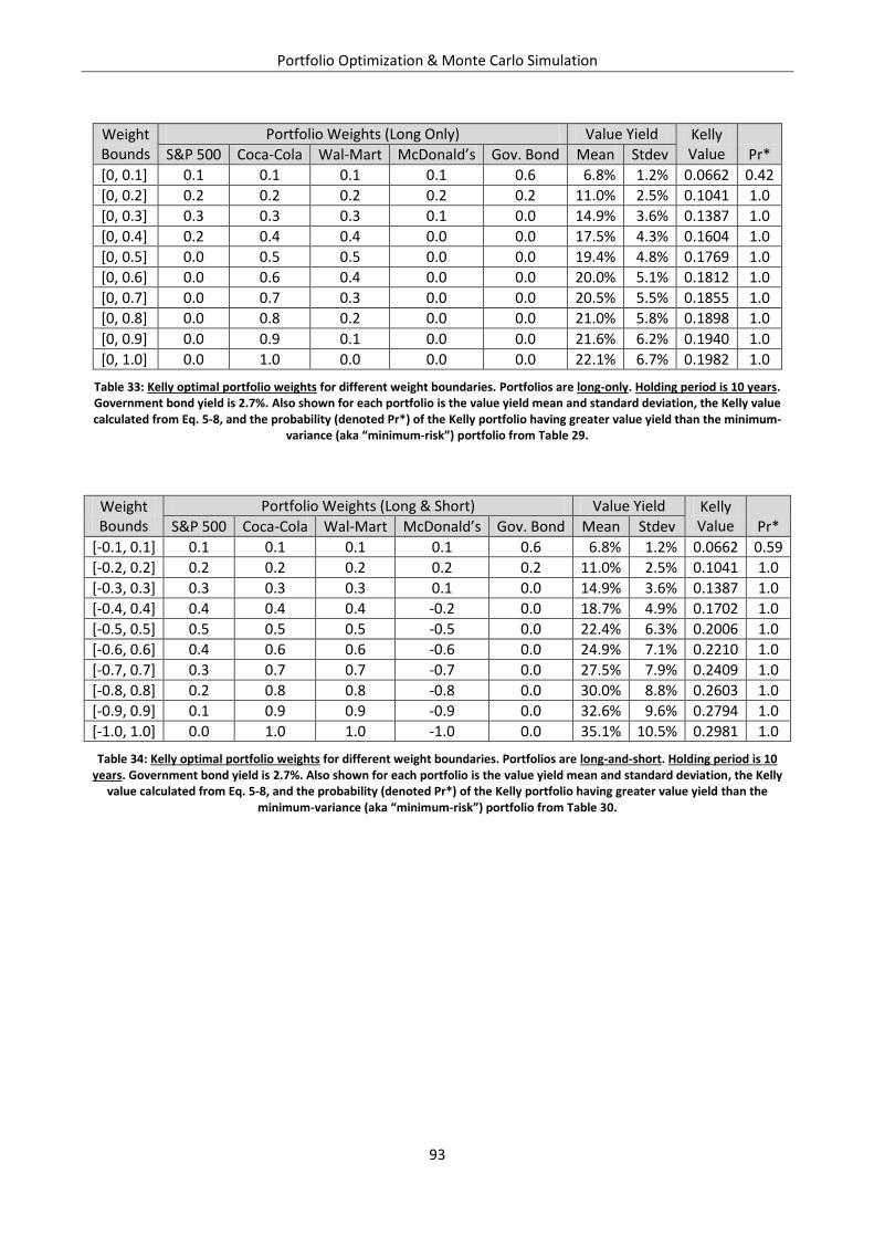
Portfolio Optimization & Monte Carlo Simulation
93
Weight Bounds
Portfolio Weights (Long Only) Value Yield Kelly Value Pr* S&P 500 Coca-Cola Wal-Mart McDonald’s Gov. Bond Mean Stdev
[0, 0.1] 0.1 0.1 0.1 0.1 0.6 6.8% 1.2% 0.0662 0.42
[0, 0.2] 0.2 0.2 0.2 0.2 0.2 11.0% 2.5% 0.1041 1.0
[0, 0.3] 0.3 0.3 0.3 0.1 0.0 14.9% 3.6% 0.1387 1.0
[0, 0.4] 0.2 0.4 0.4 0.0 0.0 17.5% 4.3% 0.1604 1.0
[0, 0.5] 0.0 0.5 0.5 0.0 0.0 19.4% 4.8% 0.1769 1.0
[0, 0.6] 0.0 0.6 0.4 0.0 0.0 20.0% 5.1% 0.1812 1.0
[0, 0.7] 0.0 0.7 0.3 0.0 0.0 20.5% 5.5% 0.1855 1.0
[0, 0.8] 0.0 0.8 0.2 0.0 0.0 21.0% 5.8% 0.1898 1.0
[0, 0.9] 0.0 0.9 0.1 0.0 0.0 21.6% 6.2% 0.1940 1.0
[0, 1.0] 0.0 1.0 0.0 0.0 0.0 22.1% 6.7% 0.1982 1.0
Table 33: Kelly optimal portfolio weights for different weight boundaries. Portfolios are long-only. Holding period is 10 years. Government bond yield is 2.7%. Also shown for each portfolio is the value yield mean and standard deviation, the Kelly value calculated from Eq. 5-8, and the probability (denoted Pr*) of the Kelly portfolio having greater value yield than the minimum-
variance (aka “minimum-risk”) portfolio from Table 29.
Weight Bounds
Portfolio Weights (Long & Short) Value Yield Kelly Value Pr* S&P 500 Coca-Cola Wal-Mart McDonald’s Gov. Bond Mean Stdev
[-0.1, 0.1] 0.1 0.1 0.1 0.1 0.6 6.8% 1.2% 0.0662 0.59
[-0.2, 0.2] 0.2 0.2 0.2 0.2 0.2 11.0% 2.5% 0.1041 1.0
[-0.3, 0.3] 0.3 0.3 0.3 0.1 0.0 14.9% 3.6% 0.1387 1.0
[-0.4, 0.4] 0.4 0.4 0.4 -0.2 0.0 18.7% 4.9% 0.1702 1.0
[-0.5, 0.5] 0.5 0.5 0.5 -0.5 0.0 22.4% 6.3% 0.2006 1.0
[-0.6, 0.6] 0.4 0.6 0.6 -0.6 0.0 24.9% 7.1% 0.2210 1.0
[-0.7, 0.7] 0.3 0.7 0.7 -0.7 0.0 27.5% 7.9% 0.2409 1.0
[-0.8, 0.8] 0.2 0.8 0.8 -0.8 0.0 30.0% 8.8% 0.2603 1.0
[-0.9, 0.9] 0.1 0.9 0.9 -0.9 0.0 32.6% 9.6% 0.2794 1.0
[-1.0, 1.0] 0.0 1.0 1.0 -1.0 0.0 35.1% 10.5% 0.2981 1.0
Table 34: Kelly optimal portfolio weights for different weight boundaries. Portfolios are long-and-short. Holding period is 10 years. Government bond yield is 2.7%. Also shown for each portfolio is the value yield mean and standard deviation, the Kelly
value calculated from Eq. 5-8, and the probability (denoted Pr*) of the Kelly portfolio having greater value yield than the minimum-variance (aka “minimum-risk”) portfolio from Table 30.
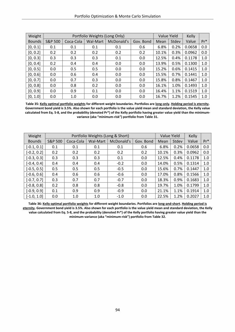
Portfolio Optimization & Monte Carlo Simulation
94
Weight Bounds
Portfolio Weights (Long Only) Value Yield Kelly Value Pr* S&P 500 Coca-Cola Wal-Mart McDonald’s Gov. Bond Mean Stdev
[0, 0.1] 0.1 0.1 0.1 0.1 0.6 6.8% 0.2% 0.0658 0.0
[0, 0.2] 0.2 0.2 0.2 0.2 0.2 10.1% 0.3% 0.0962 0.0
[0, 0.3] 0.3 0.3 0.3 0.1 0.0 12.5% 0.4% 0.1178 1.0
[0, 0.4] 0.2 0.4 0.4 0.0 0.0 13.9% 0.5% 0.1300 1.0
[0, 0.5] 0.0 0.5 0.5 0.0 0.0 15.2% 0.6% 0.1415 1.0
[0, 0.6] 0.0 0.6 0.4 0.0 0.0 15.5% 0.7% 0.1441 1.0
[0, 0.7] 0.0 0.7 0.3 0.0 0.0 15.8% 0.8% 0.1467 1.0
[0, 0.8] 0.0 0.8 0.2 0.0 0.0 16.1% 1.0% 0.1493 1.0
[0, 0.9] 0.0 0.9 0.1 0.0 0.0 16.4% 1.1% 0.1519 1.0
[0, 1.0] 0.0 1.0 0.0 0.0 0.0 16.7% 1.2% 0.1545 1.0
Table 35: Kelly optimal portfolio weights for different weight boundaries. Portfolios are long-only. Holding period is eternity. Government bond yield is 3.5%. Also shown for each portfolio is the value yield mean and standard deviation, the Kelly value calculated from Eq. 5-8, and the probability (denoted Pr*) of the Kelly portfolio having greater value yield than the minimum-
variance (aka “minimum-risk”) portfolio from Table 31.
Weight Bounds
Portfolio Weights (Long & Short) Value Yield Kelly Value Pr* S&P 500 Coca-Cola Wal-Mart McDonald’s Gov. Bond Mean Stdev
[-0.1, 0.1] 0.1 0.1 0.1 0.1 0.6 6.8% 0.2% 0.0658 0.0
[-0.2, 0.2] 0.2 0.2 0.2 0.2 0.2 10.1% 0.3% 0.0962 0.0
[-0.3, 0.3] 0.3 0.3 0.3 0.1 0.0 12.5% 0.4% 0.1178 1.0
[-0.4, 0.4] 0.4 0.4 0.4 -0.2 0.0 14.0% 0.5% 0.1314 1.0
[-0.5, 0.5] 0.5 0.5 0.5 -0.5 0.0 15.6% 0.7% 0.1447 1.0
[-0.6, 0.6] 0.4 0.6 0.6 -0.6 0.0 17.0% 0.8% 0.1566 1.0
[-0.7, 0.7] 0.3 0.7 0.7 -0.7 0.0 18.3% 0.9% 0.1683 1.0
[-0.8, 0.8] 0.2 0.8 0.8 -0.8 0.0 19.7% 1.0% 0.1799 1.0
[-0.9, 0.9] 0.1 0.9 0.9 -0.9 0.0 21.1% 1.1% 0.1914 1.0
[-1.0, 1.0] 0.0 1.0 1.0 -1.0 0.0 22.5% 1.2% 0.2027 1.0
Table 36: Kelly optimal portfolio weights for different weight boundaries. Portfolios are long-and-short. Holding period is eternity. Government bond yield is 3.5%. Also shown for each portfolio is the value yield mean and standard deviation, the Kelly
value calculated from Eq. 5-8, and the probability (denoted Pr*) of the Kelly portfolio having greater value yield than the minimum-variance (aka “minimum-risk”) portfolio from Table 32.

Portfolio Optimization & Monte Carlo Simulation
95
14. Bibliography
[1] H. Markowitz, "Portfolio Selection," Journal of Finance, vol. 7, no. 1, pp. 77-91, 1952.
[2] H. Markowitz, Portfolio Selection, Efficient Diversification of Investments.: John Wiley & Sons, 1959.
[3] M.E.H. Pedersen, "Monte Carlo Simulation in Financial Valuation," Hvass Laboratories, HL-1302, 2013.
[Online]. http://www.hvass-labs.org/people/magnus/publications/pedersen2013monte-carlo.pdf
[4] J.L. Kelly, "A New Interpretation of Information Rate," Bell System Technical Journal, vol. 35, pp. 917-
926, July 1956.
[5] J.B. Williams, The Theory of Investment Value.: Harvard University Press, 1938.
[6] M.E.H. Pedersen, "Introduction to Share Buyback Valuation," Hvass Laboratories, Report HL-1301,
2013. [Online]. http://www.hvass-labs.org/people/magnus/publications/pedersen2013share-buyback-
intro.pdf
[7] M.E.H. Pedersen, "The Value of Share Buybacks," Hvass Laboratories, Report HL-1201, 2012. [Online].
http://www.hvass-labs.org/people/magnus/publications/pedersen2012share-buyback.pdf
[8] D.G. Luenberger, Investment Science.: Oxford University Press, 1998.
[9] L.C MacLean, E.O. Thorp, and W.T. Ziemba, "Good and bad properties of the Kelly criterion," 2010.
[10] R. Storn and K. Price, "Differential evolution - a simple and efficient heuristic for global optimization
over continuous spaces," Journal of Global Optimization, vol. 11, pp. 341-359, 1997.
[11] M.E.H. Pedersen, "Good Parameters for Differential Evolution," Hvass Laboratories, Technical Report
HL1002, 2010.
[12] S. Homer and R. Sylla, A History of Interest Rates, 4th ed.: John Wiley & Sons, 2005.

Portfolio Optimization & Monte Carlo Simulation
96
15. Revision History 2014, August 3: Minor revisions. (96 pages)
2014, May 28: Added sections 5 and 11.3. Extended section 11.1.4. Minor revisions. (96 pages)
2014, May 17: First edition. (83 pages)