Embed Size (px)
Citation preview
Monte Carlo Standard Errors for Markov Chain Monte Carlo
a dissertationsubmitted to the faculty of the graduate school
of the university of minnesotaby
James Marshall Flegal
in partial fulfillment of the requirementsfor the degree of
doctor of philosophy
Galin L. Jones andGlen D. Meeden, Advisers
July 2008


c© James Marshall Flegal 2008


Acknowledgements
I would like to thank my adviser Galin Jones for his guidance, friendship, encourage-
ment, and patience throughout my studies at the University of Minnesota. Beginning
my first day of class through final corrections on my thesis, Galin challenged me to
always continue to learn. Fortunately, I’ve come a long way since that first day, and I
look forward to continuing the journey. I would also like to thank my other committee
members Glen Meeden, Charlie Geyer, and Jim Hodges for their research guidance
during my final two years. Without their generous support, this would not have been
possible.
I also owe a debt of gratitude to the faculty, staff, and fellow students in the School
of Statistics during my time at Minnesota. In particularly, I would like to thank Gary
Oehlert, the Director of Graduate Studies who saw potential in an unusual application
to the School of Statistics.
I an extremely grateful to the Kalamazoo Foundation, specifically all of the con-
tributors to the Clarence L. Remynse Scholarship whose aid was greatly appreciated.
Finally, I am thankful to both friends and family whose support helped me get
through the good and bad times during my years in Minnesota. I am especially
grateful to Amanda Isaacson for her daily support and encourage, particularly during
the final days writing my thesis.
Thank you, endless gratitude is due to all of you.
i


Abstract
Markov chain Monte Carlo (MCMC) is a method of producing a correlated sample
to estimate characteristics of a target distribution. A fundamental question is how
long should the simulation be run? One method to address this issue is to run the
simulation until the width of a confidence interval for the quantity of interest is below
a user-specified value. The use of this fixed-width methods requires an estimate of
the Monte Carlo standard error (MCSE). This dissertation begins by discussing why
MCSEs are important, how they can be easily calculated in MCMC and how they can
be used to decide when to stop the simulation. The use of MCSEs is then compared
to a popular alternative in the context of multiple examples.
This dissertation continues by discussing the relevant Markov chain theory with
particular attention paid to the conditions and definitions needed to establish a
Markov chain central limit theorem. Estimating MCSEs requires estimating the as-
sociated asymptotic variance. I introduce several techniques for estimating MCSEs:
batch means, overlapping batch means, regeneration, subsampling and spectral vari-
ance estimation. Asymptotic properties useful in MCMC settings are established for
these variance estimators. Specifically, I established conditions under which the esti-
mator for the asymptotic variance in a Markov chain central limit theorem is strongly
consistent. Strong consistency ensures that confidence intervals formed will be asymp-
totically valid. In addition, I established conditions to ensure mean-square consistency
for the estimators using batch means and overlapping batch means. Mean-square con-
iii

iv
sistency is useful in choosing an optimal batch size for MCMC practitioners.
Several approaches have been introduced dealing with the special case of estimat-
ing ergodic averages and their corresponding standard errors. Surprisingly, very little
attention has been given to characteristics of the target distribution that cannot be
represented as ergodic averages. To this end, I proposed use of subsampling methods
as a means for estimating the qth quantile of the posterior distribution. Finally, the
finite sample properties of subsampling are examined.
Contents
1 Motivation 1
1.1 Introduction . . . . . . . . . . . . . . . . . . . . . . . . . . . . . . . . 1
1.2 Markov Chain Basics . . . . . . . . . . . . . . . . . . . . . . . . . . . 3
1.3 Monte Carlo Error . . . . . . . . . . . . . . . . . . . . . . . . . . . . 4
1.3.1 Batch Means . . . . . . . . . . . . . . . . . . . . . . . . . . . 6
1.3.2 How Many Significant Figures? . . . . . . . . . . . . . . . . . 7
1.4 Stopping the Simulation . . . . . . . . . . . . . . . . . . . . . . . . . 9
1.4.1 Fixed-Width Methods . . . . . . . . . . . . . . . . . . . . . . 10
1.4.2 The Gelman-Rubin Diagnostic . . . . . . . . . . . . . . . . . . 14
1.5 Hierarchical Model . . . . . . . . . . . . . . . . . . . . . . . . . . . . 20
1.6 Discussion . . . . . . . . . . . . . . . . . . . . . . . . . . . . . . . . . 23
1.7 Proofs and Calculations . . . . . . . . . . . . . . . . . . . . . . . . . 24
1.7.1 Toy Example . . . . . . . . . . . . . . . . . . . . . . . . . . . 24
1.7.2 More on the Gelman-Rubin Diagnostic . . . . . . . . . . . . . 30
2 Markov Chain Monte Carlo 33
2.1 Markov Chains . . . . . . . . . . . . . . . . . . . . . . . . . . . . . . 33
2.1.1 Establishing Geometric Ergodicity . . . . . . . . . . . . . . . . 37
2.2 MCMC . . . . . . . . . . . . . . . . . . . . . . . . . . . . . . . . . . . 41
2.3 Examples . . . . . . . . . . . . . . . . . . . . . . . . . . . . . . . . . 43
v
vi Contents
2.3.1 Hierarchical Linear Mixed Models . . . . . . . . . . . . . . . . 43
2.4 Proofs and Calculations . . . . . . . . . . . . . . . . . . . . . . . . . 46
2.4.1 Proof of Lemma 2 . . . . . . . . . . . . . . . . . . . . . . . . . 46
2.4.2 Mixing Conditions . . . . . . . . . . . . . . . . . . . . . . . . 47
2.4.3 Block Gibbs Sampler . . . . . . . . . . . . . . . . . . . . . . . 51
3 Monte Carlo Error 59
3.1 Introduction . . . . . . . . . . . . . . . . . . . . . . . . . . . . . . . . 60
3.1.1 Stopping the Simulation . . . . . . . . . . . . . . . . . . . . . 60
3.2 Variance Estimation . . . . . . . . . . . . . . . . . . . . . . . . . . . 63
3.2.1 Notation and Assumptions . . . . . . . . . . . . . . . . . . . . 64
3.2.2 Spectral Density Estimation . . . . . . . . . . . . . . . . . . . 65
3.2.3 Batch Means . . . . . . . . . . . . . . . . . . . . . . . . . . . 69
3.2.4 Regeneration . . . . . . . . . . . . . . . . . . . . . . . . . . . 75
3.3 Examples . . . . . . . . . . . . . . . . . . . . . . . . . . . . . . . . . 78
3.3.1 AR(1) Model . . . . . . . . . . . . . . . . . . . . . . . . . . . 78
3.3.2 Bayesian Probit Regression . . . . . . . . . . . . . . . . . . . 83
3.3.3 Summary . . . . . . . . . . . . . . . . . . . . . . . . . . . . . 89
3.4 Proofs and Calculations . . . . . . . . . . . . . . . . . . . . . . . . . 90
3.4.1 Results for Proof of Lemma 4 . . . . . . . . . . . . . . . . . . 90
3.4.2 Results for Proof of Theorem 5 . . . . . . . . . . . . . . . . . 93
3.4.3 Results for Proof of Proposition 2 . . . . . . . . . . . . . . . . 105
3.4.4 Results for Mean-Square Consistency . . . . . . . . . . . . . . 109
4 Subsampling 115
4.1 Introduction . . . . . . . . . . . . . . . . . . . . . . . . . . . . . . . . 115
4.1.1 Non-overlapping Block Bootstrap . . . . . . . . . . . . . . . . 117
4.1.2 Subsampling . . . . . . . . . . . . . . . . . . . . . . . . . . . . 119
Contents vii
4.2 Stopping the Simulation . . . . . . . . . . . . . . . . . . . . . . . . . 123
4.2.1 Fixed-Width Methods . . . . . . . . . . . . . . . . . . . . . . 123
4.2.2 The Gelman-Rubin Diagnostic . . . . . . . . . . . . . . . . . . 126
4.3 Examples . . . . . . . . . . . . . . . . . . . . . . . . . . . . . . . . . 130
4.3.1 Toy Example Continued . . . . . . . . . . . . . . . . . . . . . 130
4.3.2 Block Gibbs Numerical Example . . . . . . . . . . . . . . . . 132
4.3.3 Discussion . . . . . . . . . . . . . . . . . . . . . . . . . . . . . 137
A Supplementary Material 139
A.1 Brownian Motion . . . . . . . . . . . . . . . . . . . . . . . . . . . . . 139
A.1.1 Results for Spectral Variance . . . . . . . . . . . . . . . . . . 140
A.1.2 Results for Overlapping Batch Means . . . . . . . . . . . . . . 148
A.1.3 Results for Batch Means . . . . . . . . . . . . . . . . . . . . . 157
A.1.4 Results for Mean Square Consistency . . . . . . . . . . . . . . 158
References 173


List of Tables
1.1 Summary of the proportion (and standard error) of the observed esti-
mates which were based on the minimum number (400) of draws, less
than or equal to 1000 draws, and the average total simulation effort
for the toy example in Section 1.3.2. . . . . . . . . . . . . . . . . . . . 12
1.2 Summary table for all settings and estimated mean-squared-error for
estimating E(µ|y) and E(λ|y) for the toy example of Section 1.3.2.
Standard errors (S.E.) shown for each estimate. . . . . . . . . . . . . 17
1.3 Summary of estimated mean-squared error obtained using BM and
GRD for the model of Section 1.5. Standard errors (S.E.) shown for
each estimate. . . . . . . . . . . . . . . . . . . . . . . . . . . . . . . . 22
3.1 Table of coverage probabilities for 2000 replications using the AR(1)
example with ρ = 0.5. All calculations were based on the nominal level
of 0.95. The standard errors for these numbers are easily calculated as√p(1− p)/2000 which results in a largest standard error of 6.4e-3. . . 80
3.2 Table of mean confidence interval half-widths with standard errors for
2000 replications using the AR(1) example with ρ = 0.5. . . . . . . . 81
ix
x List of Tables
3.3 Table of coverage probabilities for 2000 replications using the AR(1)
example with ρ = 0.95. All calculations were based on the nominal
level of 0.95. The standard errors for these numbers are easily calcu-
lated as√p(1− p)/2000 which results in a largest standard error of
0.011. . . . . . . . . . . . . . . . . . . . . . . . . . . . . . . . . . . . 81
3.4 Table of mean confidence interval half-widths with standard errors for
2000 replications using the AR(1) example with ρ = 0.95. . . . . . . . 82
3.5 Results from 9e6 iterations for the Bayesian probit regression using the
Lupus data from van Dyk and Meng (2001). These values were treated
as the “truth” for estimating confidence interval coverage probabilities. 84
3.6 Summary of results for using fixed-width methods for the Lupus data
Bayesian probit regression. Coverage probabilities using calculated
half-width have MCSEs of 1.4e-2 when bn = bn1/3c and between 7.7e-3
and 8.5e-3 when bn = bn1/2c. The table also shows the mean simula-
tion effort at termination in terms of number of iterations. The mean
confidence interval lengths reported all have MCSEs below 2e-4. . . . 86
3.7 Summary of results for using fixed-width methods with a Bonferonni
correction for the Lupus data Bayesian probit regression. Coverage
probabilities using calculated half-width have MCSEs of between 1.1e-
2 and 1.3e-2 when bn = bn1/3c and between 4.6e-3 and 6.3e-3 when bn =
bn1/2c. The table also shows the mean simulation effort at termination
in terms of number of iterations. The mean confidence interval lengths
reported all have MCSEs below 1e-4. . . . . . . . . . . . . . . . . . . 87
3.8 Coverage probabilities and mean confidence interval lengths comparing
BM, OBM, and SV using 7e5 Iterations to RS. MCSEs vary between
6.6e-3 and 7.7e-3 for the coverage probabilities and are less that 3e-4
for the mean interval lengths. . . . . . . . . . . . . . . . . . . . . . . 88

List of Tables xi
4.1 Summary of the proportion of replications when the true parameter
value fell within a parametric and non-parametric confidence interval
for estimating M and L for the Toy Example. . . . . . . . . . . . . . 127
4.2 Summary table for all settings and estimated mean-squared-error for
estimating M and L for the toy example of Section 1.3.2. . . . . . . . 129
4.3 Summary of the proportion (and standard error) of the observed esti-
mates which were based on the minimum number (400) of draws, less
than or equal to 1000 draws, and the average total simulation effort
for the toy example in Section 1.3.2. . . . . . . . . . . . . . . . . . . . 130
4.4 Simulated data for block Gibbs example. . . . . . . . . . . . . . . . . 132
4.5 Estimates for the nine quantities in the hierarchical example in Sec-
tion 2.3.1. Calculations from BM are based on 4×10⁶ iterations in the
chain and subsampling calculations are based on 250,000 iterations in
the chain. The standard errors (S.E.) for each of the observed quanti-
ties are included. . . . . . . . . . . . . . . . . . . . . . . . . . . . . . 133
4.6 Summary table for all settings considered in the hierarchical example
in Section 2.3.1. This table also gives the mean observed value of the
half-width and number of iterations. Both are reported with standard
errors in the additional column. . . . . . . . . . . . . . . . . . . . . . 134
4.7 Summary of replications for estimating the nine parameters of interest
for the Hierarchical example in Section 2.3.1 based on 500 independent
replications. Standard errors (S.E.) are listed for each of the quantities. 135


List of Figures
1.1 Histograms from 1000 replications estimating E(µ|y) for the toy ex-
ample of Section 1.3.2 with BM and GRD. Simulation sample sizes are
given in Table 1.1. . . . . . . . . . . . . . . . . . . . . . . . . . . . . 13
1.2 Estimating E(µ|y) for the toy example of Section 1.3.2. Estimates of
E(µ|y) versus number of draws for the BM2 and GRD4 settings. . . . 18
3.1 Plot of σ versus the number of iterations in the chain using BM, OBM,
TH, and Brt for the AR(1) model with ν = 1/2. The solid black lines
represent the actual values of σg. . . . . . . . . . . . . . . . . . . . . 79
4.1 Plots illustrating non-overlapping bootstrap resampling for time–series
data using the AR(1) model. . . . . . . . . . . . . . . . . . . . . . . . 118
4.2 Histograms from 1000 replications estimating M for the toy example
of Section 1.3.2 with SUB and GRD. Simulation sample sizes are given
in Table 4.3. . . . . . . . . . . . . . . . . . . . . . . . . . . . . . . . . 125
4.3 Estimating M for the toy example of Section 1.3.2. Estimates of M
versus number of draws for the SUB2 and GRD4 settings. . . . . . . 127
xiii


Chapter 1
Motivation: Can We Trust theThird Significant Figure?
Current reporting of results based on Markov chain Monte Carlo computations could
be improved. In particular, a measure of the accuracy of the resulting estimates
is rarely reported. Thus we have little ability to objectively assess the quality of
the reported estimates. We address this issue in that we discuss why Monte Carlo
standard errors are important, how they can be easily calculated in Markov chain
Monte Carlo and how they can be used to decide when to stop the simulation. We
compare their use to a popular alternative in the context of two examples.
The content of this chapter is primarily contained in Flegal et al. (2008) and
serves as an introduction to the problem of interest. The results here are expanded
and formalized in subsequent chapters.
1.1 Introduction
Hoaglin and Andrews (1975) consider the general problem of what information should
be included in publishing computation-based results. The goal of their suggestions
was “...to make it easy for the reader to make reasonable assessments of the numerical
quality of the results.” In particular, Hoaglin and Andrews suggested that it is crucial
1

2 Chapter 1. Motivation
to report some notion of the accuracy of the results and, for Monte Carlo studies this
should include estimated standard errors. However, in settings where Markov chain
Monte Carlo (MCMC) is used there is a culture of rarely reporting such information.
For example, we looked at the issues published in 2006 of Journal of the American
Statistical Association, Biometrika and Journal of the Royal Statistical Society, Series
B. In these journals we found 39 papers that used MCMC. Only 3 of them directly
addressed the Monte Carlo error in the reported estimates. Thus it is apparent that
the readers of the other papers have little ability to objectively assess the quality
of the reported estimates. We attempt to address this issue in that we discuss why
Monte Carlo standard errors are important, how they can be easily calculated in
MCMC settings and compare their use to a popular alternative.
Simply put, MCMC is a method for using a computer to generate data and subse-
quently using standard large sample statistical methods to estimate fixed, unknown
quantities of a given target distribution. (Thus, we object to calling it ‘Bayesian
Computation’.) That is, it is used to produce a point estimate of some characteristic
of a target distribution π having support X. The most common use of MCMC is to
estimate Eπg :=∫
Xg(x)π(dx) where g is a real-valued, π-integrable function on X.
Suppose that X = X1, X2, X3, . . . is an aperiodic, irreducible, positive Harris
recurrent Markov chain with state space X and invariant distribution π (for definitions
see Section 2.1). In this case X is Harris ergodic. Typically, estimating Eπg is
natural since an appeal to the Ergodic Theorem implies that if Eπ|g| <∞ then, with
probability 1,
gn :=1
n
n∑i=1
g(Xi) → Eπg as n→∞.
The MCMC method entails constructing a Markov chain X satisfying the regularity
conditions described above and then simulating X for a finite number of steps, say
n, and using gn to estimate Eπg. The popularity of MCMC largely is due to the ease

1.2. Markov Chain Basics 3
with which such an X can be simulated (Chen et al., 2000; Robert and Casella, 1999;
Liu, 2001).
An obvious question is when should we stop the simulation? That is, how large
should n be? Or, when is gn a good estimate of Eπg? In a given application we
usually have an idea about how many significant figures we want in our estimate but
how should this be assessed? Responsible statisticians and scientists want to do the
right thing but output analysis in MCMC has become a muddled area with often
conflicting advice and dubious terminology. This leaves many in a position where
they feel forced to rely on intuition, folklore and heuristics. We believe this often
leads to some poor practices: (A) Stopping the simulation too early, (B) Wasting
potentially useful samples, and, most importantly, (C) Providing no notion of the
quality of gn as an estimate of Eπg. In this thesis we focus on issue (C) but touch
briefly on (A) and (B).
The rest of this chapter is organized as follows. In Section 1.2 we briefly introduce
some basic concepts from the theory of Markov chains. In Section 1.3 we consider
estimating the Monte Carlo error of gn. Then Section 1.4 covers two methods for
stopping the simulation and compares them in a toy example. In Section 1.5 the two
methods are compared again in a realistic spatial model for a data set on wheat crop
flowering dates in North Dakota. We close with some final remarks in Section 1.6.
1.2 Markov Chain Basics
Suppose that X = X1, X2, X3 . . . is a Harris ergodic Markov chain with state
space X and invariant distribution π. For n ∈ N := 1, 2, 3, . . . let P n(x, ·) be
the n-step Markov transition kernel; that is, for x ∈ X and a measurable set A,
P n(x,A) = Pr (Xn+i ∈ A | Xi = x). An extremely useful property of X is that the
4 Chapter 1. Motivation
chain will converge to the invariant distribution. Specifically,
‖P n(x, ·)− π(·)‖ ↓ 0 as n→∞,
where the left-hand side is the total variation distance between P n(x, ·) and π(·).
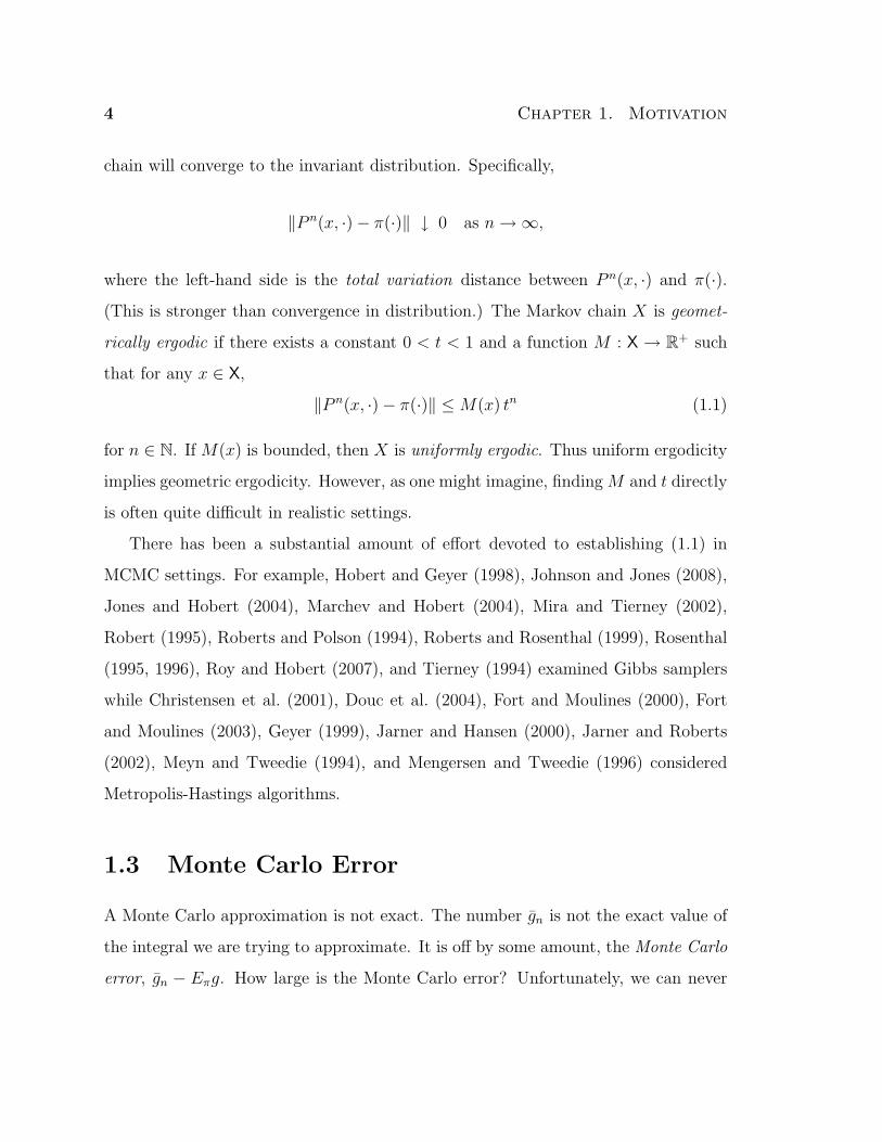
(This is stronger than convergence in distribution.) The Markov chain X is geomet-
rically ergodic if there exists a constant 0 < t < 1 and a function M : X → R+ such
that for any x ∈ X,
‖P n(x, ·)− π(·)‖ ≤M(x) tn (1.1)
for n ∈ N. If M(x) is bounded, then X is uniformly ergodic. Thus uniform ergodicity
implies geometric ergodicity. However, as one might imagine, finding M and t directly
is often quite difficult in realistic settings.
There has been a substantial amount of effort devoted to establishing (1.1) in
MCMC settings. For example, Hobert and Geyer (1998), Johnson and Jones (2008),
Jones and Hobert (2004), Marchev and Hobert (2004), Mira and Tierney (2002),
Robert (1995), Roberts and Polson (1994), Roberts and Rosenthal (1999), Rosenthal
(1995, 1996), Roy and Hobert (2007), and Tierney (1994) examined Gibbs samplers
while Christensen et al. (2001), Douc et al. (2004), Fort and Moulines (2000), Fort
and Moulines (2003), Geyer (1999), Jarner and Hansen (2000), Jarner and Roberts
(2002), Meyn and Tweedie (1994), and Mengersen and Tweedie (1996) considered
Metropolis-Hastings algorithms.
1.3 Monte Carlo Error
A Monte Carlo approximation is not exact. The number gn is not the exact value of
the integral we are trying to approximate. It is off by some amount, the Monte Carlo
error, gn − Eπg. How large is the Monte Carlo error? Unfortunately, we can never
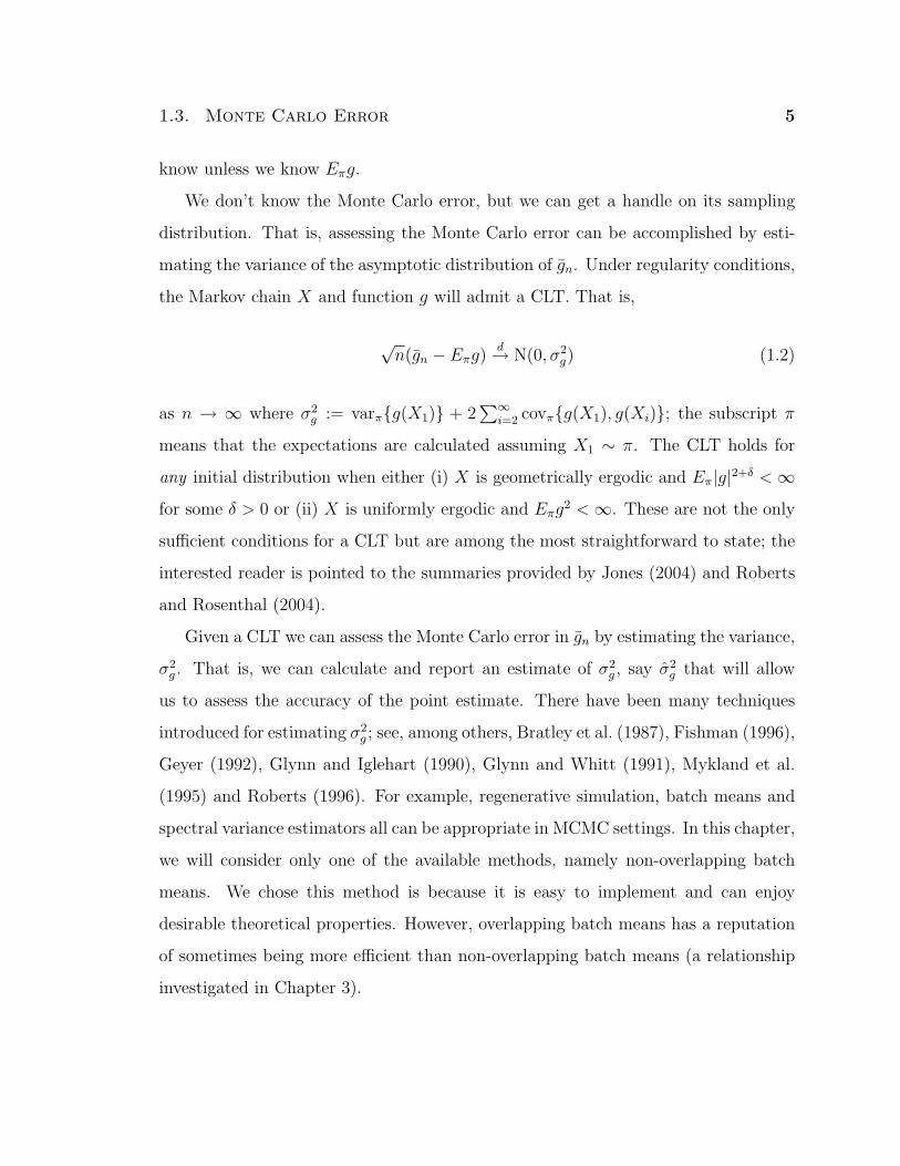
1.3. Monte Carlo Error 5
know unless we know Eπg.
We don’t know the Monte Carlo error, but we can get a handle on its sampling
distribution. That is, assessing the Monte Carlo error can be accomplished by esti-
mating the variance of the asymptotic distribution of gn. Under regularity conditions,
the Markov chain X and function g will admit a CLT. That is,
√n(gn − Eπg)
d→ N(0, σ2g) (1.2)
as n → ∞ where σ2g := varπg(X1) + 2
∑∞i=2 covπg(X1), g(Xi); the subscript π
means that the expectations are calculated assuming X1 ∼ π. The CLT holds for
any initial distribution when either (i) X is geometrically ergodic and Eπ|g|2+δ <∞
for some δ > 0 or (ii) X is uniformly ergodic and Eπg2 <∞. These are not the only
sufficient conditions for a CLT but are among the most straightforward to state; the
interested reader is pointed to the summaries provided by Jones (2004) and Roberts
and Rosenthal (2004).
Given a CLT we can assess the Monte Carlo error in gn by estimating the variance,
σ2g . That is, we can calculate and report an estimate of σ2
g , say σ2g that will allow
us to assess the accuracy of the point estimate. There have been many techniques
introduced for estimating σ2g ; see, among others, Bratley et al. (1987), Fishman (1996),
Geyer (1992), Glynn and Iglehart (1990), Glynn and Whitt (1991), Mykland et al.
(1995) and Roberts (1996). For example, regenerative simulation, batch means and
spectral variance estimators all can be appropriate in MCMC settings. In this chapter,
we will consider only one of the available methods, namely non-overlapping batch
means. We chose this method is because it is easy to implement and can enjoy
desirable theoretical properties. However, overlapping batch means has a reputation
of sometimes being more efficient than non-overlapping batch means (a relationship
investigated in Chapter 3).
6 Chapter 1. Motivation
1.3.1 Batch Means
In non-overlapping batch means the output is broken into blocks of equal size. Sup-
pose the algorithm is run for a total of n = ab iterations (hence a = an and b = bn
are implicit functions of n) and define
Yj :=1
b
jb∑i=(j−1)b+1
g(Xi) for j = 1, . . . , a .
The batch means estimate of σ2g is
σ2g =
b
a− 1
a∑j=1
(Yj − gn)2 . (1.3)
Batch means is attractive because it is easy to implement (and it is available in some
software, e.g. WinBUGS) but some authors encourage caution in its use (Roberts,
1996). In particular, we believe careful use is warranted since (1.3), in general, is not
a consistent estimator of σ2g . On the other hand, Jones et al. (2006) showed that if
the batch size and the number of batches are allowed to increase as the overall length
of the simulation increases by setting bn = bnθc and an = bn/bnc, then σ2g → σ2
g with
probability 1 as n→∞. Throughout this thesis, we consider the case consistent batch
means (BM) rather than the usual fixed number of batches version. The regularity
conditions require that X be geometrically ergodic, Eπ|g|2+δ+ε < ∞ for some δ > 0
and some ε > 0 and (1 + δ/2)−1 < θ < 1; often θ = 1/2 (i.e., bn = b√nc and
an = bn/bnc) is a convenient choice that works well in applications. Note that the
only practical difference between BM and standard batch means is that the batch
number and size are chosen as functions of the overall run length, n.
Using BM to get an estimate of the Monte Carlo standard error (MCSE) of gn,
say σg/√n, we can form an asymptotically valid confidence interval for Eπg. The

1.3. Monte Carlo Error 7
half-width of the interval is given by
tan−1σg√n
(1.4)
where tan−1 is an appropriate quantile from Student’s t distribution with an−1 degrees
of freedom.
1.3.2 How Many Significant Figures?
The title of the chapter contains a rhetorical question; we don’t always care about
the third significant figure. But we should care about how many significant figures
there are in our estimates. Assessing the Monte Carlo error through (1.4) gives us a
tool to do this. For example, suppose gn = 0.02, then there is exactly one significant
figure in the estimate, namely the “2”, but how confident are we about it? Letting hα
denote the half width given in (1.4) of a (1−α)100% interval, we would trust the one
significant figure in our estimate if 0.02 ± hα ⊆ [0.015, 0.025) since otherwise values
such as Eπg = 0.01 or Eπg = 0.03 are plausible through rounding.
More generally, we can use (1.4) to assess how many significant figures we have
in our estimates. This is illustrated in the following toy example that will be used
several times throughout the rest of this thesis.
Toy Example
Let Y1, . . . , YK be i.i.d. N(µ, λ) and let the prior for (µ, λ) be proportional to 1/√λ.
The posterior density is characterized by
π(µ, λ|y) ∝ λ−K+1
2 exp
− 1
2λ
K∑j=1
(yj − µ)2
(1.5)

8 Chapter 1. Motivation
where y = (y1, . . . , yK)T . It is easy to check that this posterior is proper as long as
K ≥ 3 and we assume this throughout. Using the Gibbs sampler to make draws
from (1.5) requires the full conditional densities, f(µ|λ, y) and f(λ|µ, y), which are
as follows:
µ|λ, y ∼ N(y, λ/K) ,
λ|µ, y ∼ IG
(K − 1
2,(K − 1)s2 +K(y − µ)2
2
),
where y is the sample mean and (K−1)s2 =∑
(yi− y)2. (We say W ∼ IG(α, β) if its
density is proportional to w−(α+1)e−β/wI(w > 0).) Consider estimating the posterior
means of µ and λ. It is easy to prove that E(µ|y) = y and E(λ|y) = (K−1)s2/(K−4)
for K > 4. Thus we do not need MCMC to estimate these quantities but we will
ignore this and use the output of a Gibbs sampler to estimate E(µ|y) and E(λ|y).
Consider the Gibbs sampler that updates λ then µ; that is, letting (λ′, µ′) denote
the current state and (λ, µ) denote the future state, the transition looks like (λ′, µ′) →
(λ, µ′) → (λ, µ). Jones and Hobert (2001) established that the associated Markov
chain is geometrically ergodic as long as K ≥ 5. If K > 10, then the moment
conditions ensuring the CLT and the regularity conditions for BM (with θ = 1/2)
hold.
Let K = 11, y = 1, and (K − 1)s2 = 14 so that E(µ|y) = 1 and E(λ|y) = 2;
for the remainder of this chapter these settings will be used every time we consider
this example. Consider estimating E(µ|y) and E(λ|y) with µn and λn, respectively
and using BM to calculate the MCSEs for each estimate. Specifically, we will use a
95% confidence level in (1.4) to construct an interval estimate. Let the initial value
for the simulation be (λ1, µ1) = (1, 1). When we ran the Gibbs sampler for 1000
iterations we obtained λ1000 = 2.003 with an MCSE of 0.055 and µ1000 = 0.99 with
an MCSE of 0.016. Thus we would be comfortable reporting two significant figures
1.4. Stopping the Simulation 9
for the estimates of E(λ|y) and E(µ|y), specifically 2.0 and 1.0, respectively. But
when we started from (λ1, µ1) = (100, 100) and ran Gibbs for 1000 iterations we
obtained λ1000 = 13.06 with an MCSE of 11.01 and µ1000 = 1.06 with an MCSE of
0.071. Thus we would not be comfortable with any significant figures for the estimate
of E(λ|y) but we would trust one significant figure (i.e., 1) for E(µ|y). Unless the
MCSE is calculated and reported a hypothetical reader would have no way to judge
this independently.
Remarks
1. A common concern about MCSEs is that their use may require estimating Eπg
much too precisely relative to√
varπg. Of course, it would be a rare problem
indeed where we would know√
varπg and not Eπg. Thus we would need to
estimate√
varπg and calculate an MCSE (via the delta method) before we
could trust the estimate of√
varπg to inform us about the MCSE for Eπg.
2. We are not suggesting that all MCMC-based estimates should be reported in
terms of significant figures; in fact we do not do this in the simulations that
occur later. Instead, we are strongly suggesting that an estimate of the Monte
Carlo standard error should be used to assess simulation error and reported.
Without an attached MCSE a point estimate should not be trusted.
1.4 Stopping the Simulation
In this section we consider two formal approaches to terminating the simulation. The
first is based on calculating an MCSE and is discussed in Section 1.4.1. The second
is based on the method introduced in Gelman and Rubin (1992) and is one of many
so-called convergence diagnostics (Cowles and Carlin, 1996). Our reason for choosing
the Gelman-Rubin diagnostic (GRD) is that it appears to be far and away the most
10 Chapter 1. Motivation
popular method for stopping the simulation. GRD and MCSE are used to stop the
simulation in a similar manner. After n iterations either the value of the GRD or
MCSE is calculated and if it isn’t sufficiently small then we continue the simulation
until it is.
1.4.1 Fixed-Width Methods
Suppose we have an idea of how many significant figures we want in our estimate.
Another way of saying this is that we want the half-width of the interval (1.4) to be
less than some user-specified value, ε. Thus we might consider stopping the simulation
when the MCSE of gn is sufficiently small. This, of course, means that we may have
to check whether this criterion is met many times. It is not obvious that such a
procedure will be guaranteed to terminate the computation in a finite amount of
time or whether the resulting intervals will enjoy the desired coverage probability and
half-width. Also, we don’t want to check too early in the simulation since we will run
the risk of premature termination due to a poor estimate of the standard error.
Suppose we use BM to estimate the Monte Carlo standard error of gn, say σg/√n,
and use it to form a confidence interval for Eπg. If this interval is too large then the
value of n is increased and simulation continues until the interval is sufficiently small.
Formally, the criterion is given by
tan−1σg√n
+ p(n) ≤ ε (1.6)
where tan−1 is an appropriate quantile, p(n) = εI(n < n∗) where, n∗ > 0 is fixed,
I is the usual indicator function on Z+ and ε > 0 is the user-specified half-width.
The role of p is to ensure that the simulation is not terminated prematurely due to
a poor estimate of σg. The conditions which guarantee σ2g is consistent also imply
that this procedure will terminate in a finite amount of time with probability one
1.4. Stopping the Simulation 11
and that the resulting intervals asymptotically have the desired coverage (see Glynn
and Whitt, 1992). However, the finite-sample properties of (1.4) have received less
formal investigation but simulation results suggest that the resulting intervals have
approximately the desired coverage and half-width in practice (see Flegal and Jones,
2008; Jones et al., 2006).
Remarks
1. The CLT and BM require a geometrically ergodic Markov chain. This can
be difficult to check directly in any given application. On the other hand,
considerable effort has been spent establishing (1.1) for a number of Markov
chains; see the references given at the end of Section 1.2. In our view, this is
not the obstacle that it was in the past.
2. The frequency with which (1.6) should be evaluated is an open question. Check-
ing often, say every few iterations, may substantially increase the overall com-
putational effort.
3. Consider p(n) = εI(n < n∗). The choice of n∗ is often made based on the
user’s experience with the problem at hand. However, for geometrically ergodic
Markov chains there is some theory that can give guidance on this issue (see
Jones and Hobert, 2001; Latuszynski, 2008; Rosenthal, 1995).
4. Stationarity of the Markov chain is not required for the CLT or the strong
consistency of BM. One consequence is that burn-in is not required if we can
find a reasonable starting value.
Toy Example
We consider implementation of fixed-width methods in the toy example introduced in
Section 1.3.2. We performed 1000 independent replications of the following procedure.
12 Chapter 1. Motivation
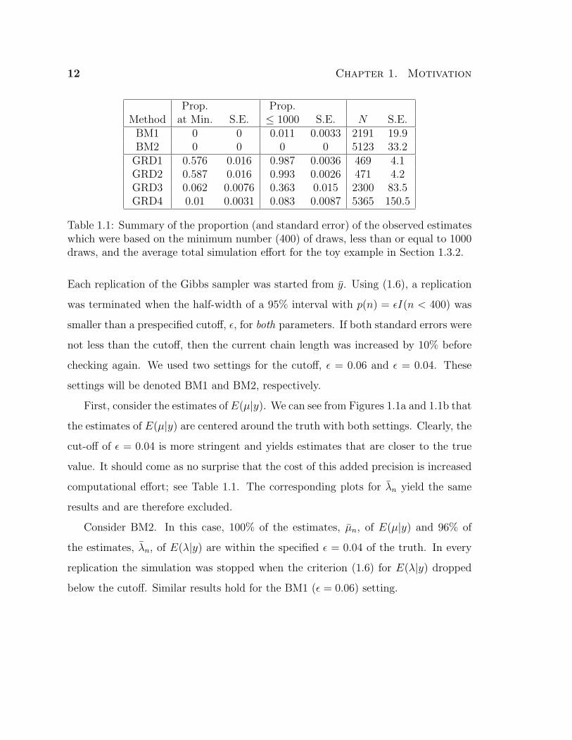
Prop. Prop.Method at Min. S.E. ≤ 1000 S.E. N S.E.BM1 0 0 0.011 0.0033 2191 19.9BM2 0 0 0 0 5123 33.2GRD1 0.576 0.016 0.987 0.0036 469 4.1GRD2 0.587 0.016 0.993 0.0026 471 4.2GRD3 0.062 0.0076 0.363 0.015 2300 83.5GRD4 0.01 0.0031 0.083 0.0087 5365 150.5
Table 1.1: Summary of the proportion (and standard error) of the observed estimateswhich were based on the minimum number (400) of draws, less than or equal to 1000draws, and the average total simulation effort for the toy example in Section 1.3.2.
Each replication of the Gibbs sampler was started from y. Using (1.6), a replication
was terminated when the half-width of a 95% interval with p(n) = εI(n < 400) was
smaller than a prespecified cutoff, ε, for both parameters. If both standard errors were
not less than the cutoff, then the current chain length was increased by 10% before
checking again. We used two settings for the cutoff, ε = 0.06 and ε = 0.04. These
settings will be denoted BM1 and BM2, respectively.
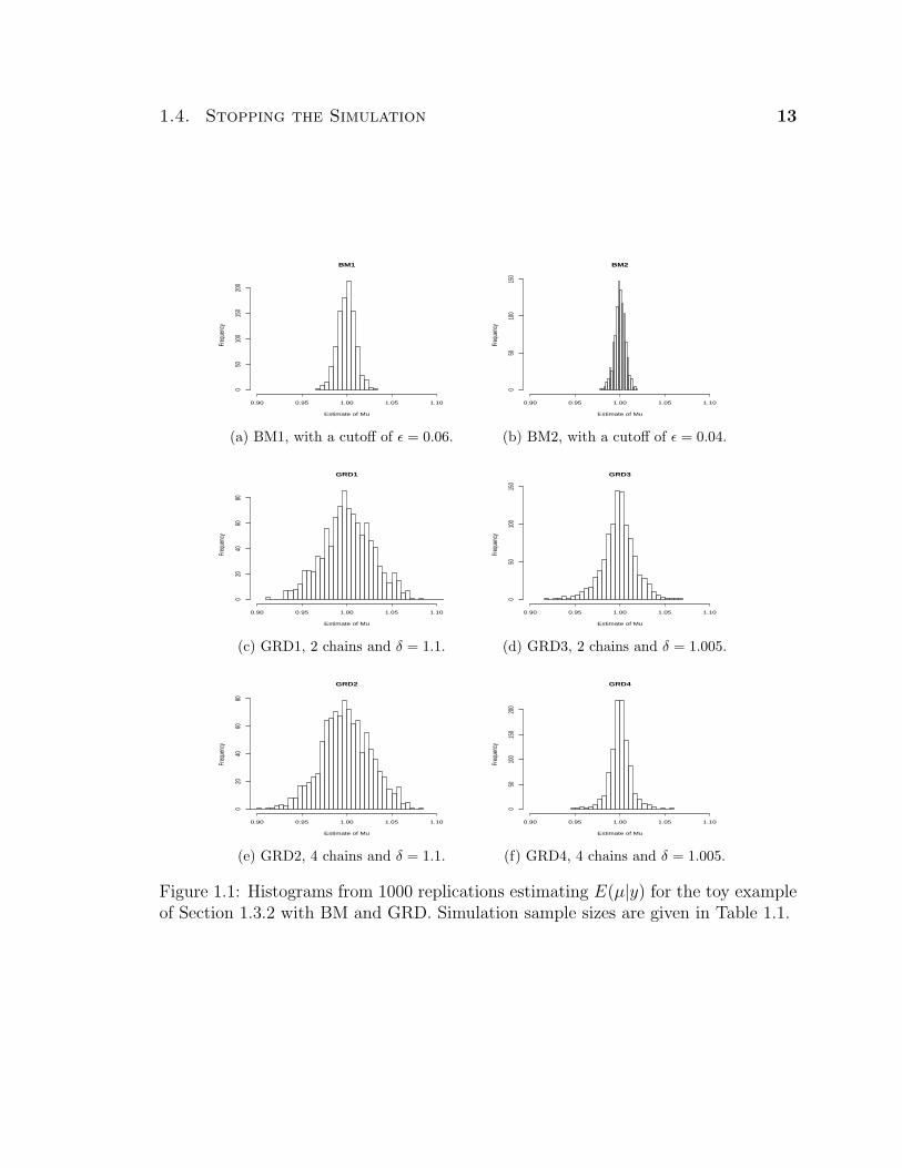
First, consider the estimates of E(µ|y). We can see from Figures 1.1a and 1.1b that
the estimates of E(µ|y) are centered around the truth with both settings. Clearly, the
cut-off of ε = 0.04 is more stringent and yields estimates that are closer to the true
value. It should come as no surprise that the cost of this added precision is increased
computational effort; see Table 1.1. The corresponding plots for λn yield the same
results and are therefore excluded.
Consider BM2. In this case, 100% of the estimates, µn, of E(µ|y) and 96% of
the estimates, λn, of E(λ|y) are within the specified ε = 0.04 of the truth. In every
replication the simulation was stopped when the criterion (1.6) for E(λ|y) dropped
below the cutoff. Similar results hold for the BM1 (ε = 0.06) setting.
1.4. Stopping the Simulation 13
BM1
Estimate of Mu
Freq
uenc
y
0.90 0.95 1.00 1.05 1.10
050
100
150
200
(a) BM1, with a cutoff of ε = 0.06.
BM2
Estimate of Mu
Freq
uenc
y
0.90 0.95 1.00 1.05 1.10
050
100
150
(b) BM2, with a cutoff of ε = 0.04.
GRD1
Estimate of Mu
Freq
uenc
y
0.90 0.95 1.00 1.05 1.10
020
4060
80
(c) GRD1, 2 chains and δ = 1.1.
GRD3
Estimate of Mu
Freq
uenc
y
0.90 0.95 1.00 1.05 1.10
050
100
150
(d) GRD3, 2 chains and δ = 1.005.
GRD2
Estimate of Mu
Freq
uenc
y
0.90 0.95 1.00 1.05 1.10
020
4060
80
(e) GRD2, 4 chains and δ = 1.1.
GRD4
Estimate of Mu
Freq
uenc
y
0.90 0.95 1.00 1.05 1.10
050
100
150
200
(f) GRD4, 4 chains and δ = 1.005.
Figure 1.1: Histograms from 1000 replications estimating E(µ|y) for the toy exampleof Section 1.3.2 with BM and GRD. Simulation sample sizes are given in Table 1.1.
14 Chapter 1. Motivation
1.4.2 The Gelman-Rubin Diagnostic
The Gelman-Rubin diagnostic (GRD) introduced in Gelman and Rubin (1992) and
refined by Brooks and Gelman (1998) is a popular method for assessing the output
of MCMC algorithms. It is important to note that this method is also based on a
Markov chain CLT (Gelman and Rubin, 1992, p.463) and hence does not apply more
generally than approaches based on calculating an MCSE.
GRD is based on the simulation of m independent parallel Markov chains having
invariant distribution π, each of length 2l. Thus the total simulation effort is 2lm.
Gelman and Rubin (1992) suggest that the first l simulations should be discarded
and inference based on the last l simulations; for the jth chain these are denoted
X1j, X2j, X3j, . . . , Xlj with j = 1, 2, . . . ,m. Recall that we are interested in esti-
mating Eπg and define Yij = g(Xij),
B =l
m− 1
m∑j=1
(Y·j − Y··)2 and W =
1
m
m∑j=1
s2j
where Y·j = l−1∑l
i=1 Yij, Y·· = m−1∑m
j=1 Y·j and s2j = (l−1)−1
∑li=1(Yij− Y·j)2. Note
that Y·· is the resulting point estimate of Eπg. Let
V =l − 1
lW +
(m+ 1)B
ml, d ≈ 2V
var(V ),
and define the corrected potential scale reduction factor
R =
√d+ 3
d+ 1
V
W.
As noted by Gelman et al. (2004), V and W are essentially two different estimators
of varπg; not σ2g from the Markov chain CLT. That is, neither V nor W address the
sampling variability of gn and hence neither does R.

1.4. Stopping the Simulation 15
In our examples we used the R package coda which reports an upper bound on R
(see Section 1.7.2). Specifically, a 97.5% upper bound for R is given by
R0.975 =
√d+ 3
d+ 1
[l − 1
l+ F0.975,m−1,w
(m+ 1
ml
B
W
)],
where F0.975,m−1,w is the 97.5% percentile of an Fm−1w distribution, w = 2W 2/σ2
W and
σ2W =
1
m− 1
m∑j=1
(s2
j −W)2
.
In order to stop the simulation the user provides a cutoff, δ > 0, and simulation
continues until
R0.975 + p(n) ≤ δ . (1.7)
As with fixed-width methods, the role of p(n) is to ensure that we do not stop the
simulation prematurely due to a poor estimate, R0.975. By requiring a minimum total
simulation effort of n∗ = 2lm we are effectively setting p(n) = δI(n < n∗) where n
indexes the total simulation effort.
Remarks
1. A rule of thumb suggested by Gelman et al. (2004) is to set δ = 1.1. These
authors also suggest that a value of δ closer to 1 will be desirable in a “final
analysis in a critical problem” but give no further guidance. Since neither R
nor R0.975 directly estimates the Monte Carlo error in gn it is unclear to us that
R ≈ 1 implies gn is a good estimate of Eπg.
2. How large should m be? There seem to be few guidelines in the literature
except that m ≥ 2 since otherwise we cannot calculate B. Clearly, if m is too
large then each chain will be too short to achieve any reasonable expectation of
16 Chapter 1. Motivation
convergence within a given computational effort.
3. The initial values, Xj1, of the m parallel chains should be drawn from an
“over-dispersed” distribution. Gelman and Rubin (1992) suggest estimating
the modes of π and then using a mixture distribution whose components are
centered at these modes. Constructing this distribution could be difficult and
is often not done in practice (Gelman et al., 2004, p. 593).
4. To our knowledge there has been no discussion in the literature about optimal
choices of p(n) or n∗. In particular, we know of no guidance about how long
each of the parallel chains should be simulated before the first time we check
that R0.975 < δ or how often one should check after that. However, the same
theoretical results that could give guidance in item 3 of Section 4.1.1 would
apply here as well.
5. GRD was originally introduced simply as a method for determining an ap-
propriate amount of burn-in. However, using diagnostics in this manner may
introduce additional bias into the results, see Cowles et al. (1999).
Toy Example
We consider implementation of GRD in the toy example introduced in Section 1.3.2.
The first issue we face is choosing the starting values for each of the m parallel chains.
Notice that
π(µ, λ|y) = g1(µ|λ)g2(λ)
where g1(µ|λ) is a N(y, λ/K) density and g2(λ) is an IG((K − 2)/2, (K − 1)s2/2)
density. Thus we can sequentially sample the exact distribution by first drawing from
g2(λ), and then conditionally, draw from g1(µ|λ). We will use this to obtain starting
values for each of the m parallel chains. Thus each of the m parallel Markov chains

1.4. Stopping the Simulation 17
Stopping MSE for MSE forMethod Chains Rule E(µ|y) S.E. E(λ|y) S.E.BM1 1 0.06 9.82e-05 4.7e-06 1.03e-03 4.5e-05BM2 1 0.04 3.73e-05 1.8e-06 3.93e-04 1.8e-05GRD1 2 1.1 7.99e-04 3.6e-05 8.7e-03 4e-04GRD2 4 1.1 7.79e-04 3.7e-05 8.21e-03 3.6e-04GRD3 2 1.005 3.49e-04 2.1e-05 3.68e-03 2e-04GRD4 4 1.005 1.34e-04 9.2e-06 1.65e-03 1.2e-04
Table 1.2: Summary table for all settings and estimated mean-squared-error for es-timating E(µ|y) and E(λ|y) for the toy example of Section 1.3.2. Standard errors(S.E.) shown for each estimate.
will be stationary and hence GRD should be at a slight advantage compared to BM
started from y.
Our goal is to investigate the finite-sample properties of the GRD by considering
the estimates of E(µ|y) and E(λ|y) as in Section 1.4.1. To this end, we took multiple
chains starting from different draws from the sequential sampler. The multiple chains
were run until the total simulation effort was n∗ = 400 draws; this is the same
minimum simulation effort we required of BM in the previous section. If R0.975 < δ
for both, the simulation was stopped. Otherwise, 10% of the current chain length was
added to each chain before R0.975 was recalculated. This continued until R0.975 was
below δ for both. This simulation procedure was repeated independently 1000 times
with each replication using the same initial values. We considered 4 settings using
the combinations of m ∈ 2, 4 and δ ∈ 1.005, 1.1. These settings will be denoted
GRD1, GRD2, GRD3 and GRD4; see Table 1.2 for the different settings along with
summary statistics that will be considered later.
Upon completion of each replication, the values of µn and λn were recorded. Fig-
ures 1c–1f show histograms of µn for each setting. We can see that all the settings
center around the true value of 1, and setting δ = 1.005 provides better estimates.
Increasing the number of chains seems to have little impact on the quality of esti-
18 Chapter 1. Motivation
0 10000 20000 30000 40000
0.95
1.00
1.05
BM2
Number of Draws
Est
imat
e of
Mu
(a) µn vs. n for BM2
0 10000 20000 30000 40000
0.95
1.00
1.05
GRD4
Number of Draws
Est
imat
e of
Mu
(b) µn vs. n for GRD4
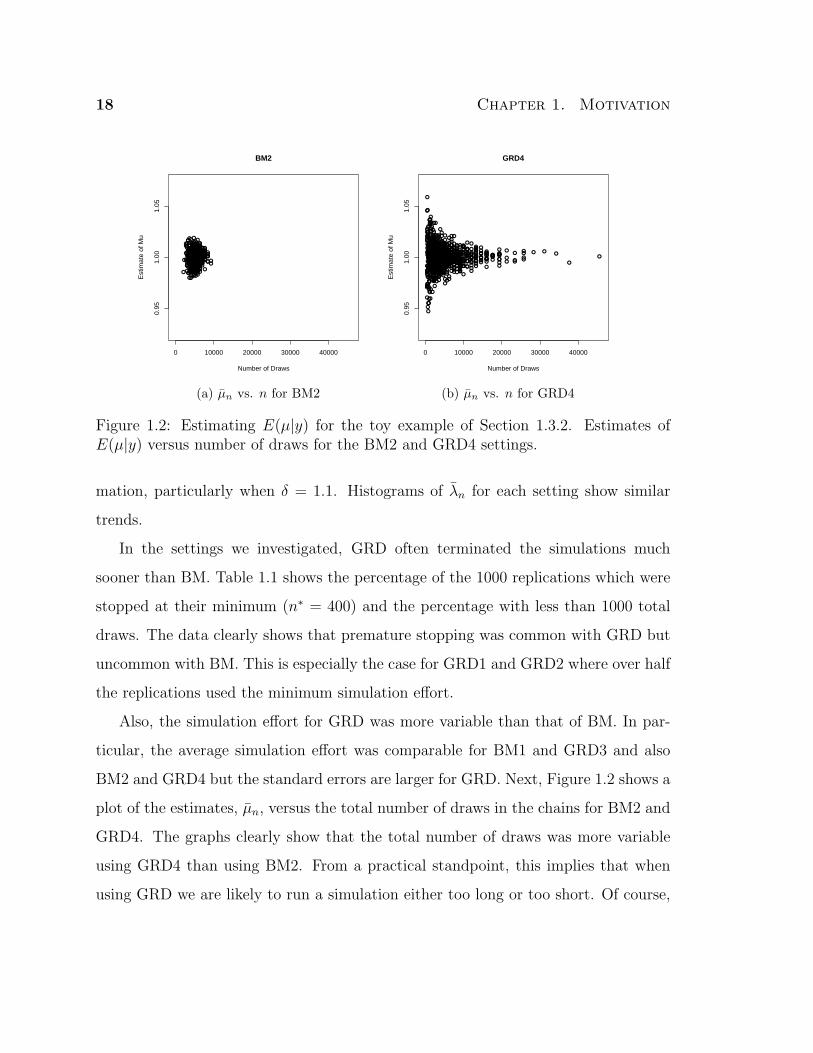
Figure 1.2: Estimating E(µ|y) for the toy example of Section 1.3.2. Estimates ofE(µ|y) versus number of draws for the BM2 and GRD4 settings.
mation, particularly when δ = 1.1. Histograms of λn for each setting show similar
trends.
In the settings we investigated, GRD often terminated the simulations much
sooner than BM. Table 1.1 shows the percentage of the 1000 replications which were
stopped at their minimum (n∗ = 400) and the percentage with less than 1000 total
draws. The data clearly shows that premature stopping was common with GRD but
uncommon with BM. This is especially the case for GRD1 and GRD2 where over half
the replications used the minimum simulation effort.
Also, the simulation effort for GRD was more variable than that of BM. In par-
ticular, the average simulation effort was comparable for BM1 and GRD3 and also
BM2 and GRD4 but the standard errors are larger for GRD. Next, Figure 1.2 shows a
plot of the estimates, µn, versus the total number of draws in the chains for BM2 and
GRD4. The graphs clearly show that the total number of draws was more variable
using GRD4 than using BM2. From a practical standpoint, this implies that when
using GRD we are likely to run a simulation either too long or too short. Of course,
1.4. Stopping the Simulation 19
if we run the simulation too long, we will be likely to get a better estimate. But if
the simulation is too short, the estimate can be poor.
Let’s compare GRD and BM in terms of the quality of estimation. Table 1.2 gives
the estimated mean-squared error (MSE) for each setting based on 1000 independent
replications described above. The estimates for GRD were obtained using the meth-
ods described earlier in this subsection while the results for BM were obtained from
the simulations performed for Section 1.4.1. It is clear that BM results in superior
estimation. In particular, note that using the setting BM1 results in better estimates
of E(µ|y) and E(λ|y) than using setting GRD4 while using approximately half the
average simulation effort (2191 (s.e. = 19.9) versus 5365 (150.5)); see Table 1.1.
Consider GRD4 and BM2. Note that these two settings have comparable average
simulation effort. The MSE for µn using GRD was 0.000134 (9.2e-6) and for BM we
observed an MSE of 0.0000373 (1.8e-6). Now consider λn. The MSE based on using
GRD was 0.00165 (1.2e-4) and for BM we observed an MSE of 0.000393 (1.8e-5).
Certainly, the more variable simulation effort of GRD contributes to this difference
but so does the default use of burn-in
Recall that we employed a sequential sampler to draw from the target distribution
implying that the Markov chain is stationary and hence burn-in is unnecessary. To
understand the effect of using burn-in we calculated the estimates of E(µ|y) using
the entire simulation; that is, we did not discard the first l draws of each of the
m parallel chains. This yields an estimated MSE of 0.0000709 (4.8e-6) for GRD4.
Thus, the estimates using GRD4 still have an estimated MSE 1.9 times larger than
that obtained using BM2. The standard errors of the MSE estimates show that this
difference is still significant, indicating BM, in terms of MSE, is still a superior method
for estimating E(µ|y). Similarly, for estimating E(λ|y) the MSE using GRD4 without
discarding the first half of each chain is 2.1 higher than that of BM2.
Toy examples are useful for illustration, however it is sometimes difficult to know
20 Chapter 1. Motivation
just how much credence the resulting claims should be given. For this reason, we turn
our attention to a setting that is “realistic” in the sense that it is similar to the type
of setting encountered in practice. Specifically, we do not know the true values of the
posterior expectations and implementing a reasonable MCMC strategy is not easy.
Moreover, we do not know the convergence rate of the associated Markov chain.
1.5 Hierarchical Model for Geostatistics
The following example is directly from Flegal et al. (2008) which considers a data
set on wheat crop flowering dates in the state of North Dakota (Haran et al., 2008).
This data consists of experts’ model-based estimates for the dates when wheat crops
flower at 365 different locations across the state. Let D be the set of N sites and the
estimate for the flowering date at site s be Z(s) for s ∈ D. Let X(s) be the latitude
for s ∈ D. The flowering dates are generally expected to be later in the year as
X(s) increases so we assume that the expected value for Z(s) increases linearly with
X(s). The flowering dates are also assumed to be spatially dependent, suggesting the
following hierarchical model:
Z(s) | β, ξ(s) = X(s)β + ξ(s) for s ∈ D ,
ξ | τ 2, σ2, φ ∼ N(0,Σ(τ 2, σ2, φ)),
where ξ = (ξ(s1), . . . , ξ(sN))T with Σ(τ 2, σ2, φ) = τ 2I + σ2H(φ) and H(φ)ij =
exp((−‖si − sj‖)/φ), the exponential correlation function. We complete the specifi-
cation of the model with priors on τ 2, σ2, φ, and β,
τ 2 ∼ IG(2, 30), σ2 ∼ IG(0.1, 30),
φ ∼ Log-Unif(0.6, 6), π(β) ∝ 1 .
1.5. Hierarchical Model 21
Setting Z = (Z(s1), . . . , Z(sN)), inference is based on the posterior distribution
π(τ 2, σ2, φ, β | Z). Note that MCMC may be required since the integrals required for
inference are analytically intractable. Also, samples from this posterior distribution
can then be used for prediction at any location s ∈ D.
Consider estimating the posterior expectation of τ 2, σ2, φ, and β. Unlike the toy
example considered earlier these expectations are not analytically available. Sampling
from the posterior is accomplished via a Metropolis-Hastings sampler with a joint
update for the τ 2, φ, β via a three-dimensional independent Normal proposal centered
at the current state with a variance of 0.3 for each component and a univariate Gibbs
update for σ2.
To obtain a high quality approximation to the desired posterior expectations we
used a single long run of 500,000 iterations of the sampler and obtained 23.23 (.0426),
25.82 (.0200), 2.17 (.0069), and 4.09 (4.3e-5) as estimates of the posterior expectations
of τ 2, σ2, φ, and β, respectively. These are assumed to be the truth. We also recorded
the 10th, 30th, 70th and 90th percentiles of this long run for each parameter.
Our goal is to compare the finite-sample properties of GRD and BM in terms
of quality of estimation and overall simulation effort. Consider implementation of
GRD. We will produce 100 independent replications using the following procedure.
For each replication we used m = 4 parallel chains from four different starting values
corresponding to the 10th, 30th, 70th and 90th percentiles recorded above. A mini-
mum total simulation effort of 1000 (250 per chain) was required. Also, no burn-in
was employed. This is consistent with our finding in the toy example that estimation
improved without using burn-in. Each replication continued until R0.975 ≤ 1.1 for all
of the parameter estimates. Estimates of the posterior expectations were obtained by
averaging draws across all 4 parallel chains.
Now consider the implementation of BM. For the purpose of easy comparison with
GRD, we ran a total of 400 independent replications of our MCMC sampler, where the
22 Chapter 1. Motivation
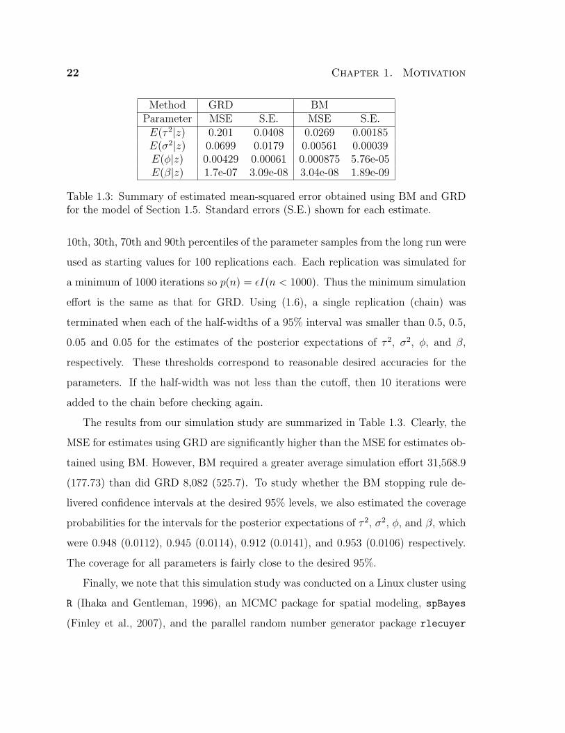
Method GRD BMParameter MSE S.E. MSE S.E.E(τ 2|z) 0.201 0.0408 0.0269 0.00185E(σ2|z) 0.0699 0.0179 0.00561 0.00039E(φ|z) 0.00429 0.00061 0.000875 5.76e-05E(β|z) 1.7e-07 3.09e-08 3.04e-08 1.89e-09
Table 1.3: Summary of estimated mean-squared error obtained using BM and GRDfor the model of Section 1.5. Standard errors (S.E.) shown for each estimate.
10th, 30th, 70th and 90th percentiles of the parameter samples from the long run were
used as starting values for 100 replications each. Each replication was simulated for
a minimum of 1000 iterations so p(n) = εI(n < 1000). Thus the minimum simulation
effort is the same as that for GRD. Using (1.6), a single replication (chain) was
terminated when each of the half-widths of a 95% interval was smaller than 0.5, 0.5,
0.05 and 0.05 for the estimates of the posterior expectations of τ 2, σ2, φ, and β,
respectively. These thresholds correspond to reasonable desired accuracies for the
parameters. If the half-width was not less than the cutoff, then 10 iterations were
added to the chain before checking again.
The results from our simulation study are summarized in Table 1.3. Clearly, the
MSE for estimates using GRD are significantly higher than the MSE for estimates ob-
tained using BM. However, BM required a greater average simulation effort 31,568.9
(177.73) than did GRD 8,082 (525.7). To study whether the BM stopping rule de-
livered confidence intervals at the desired 95% levels, we also estimated the coverage
probabilities for the intervals for the posterior expectations of τ 2, σ2, φ, and β, which
were 0.948 (0.0112), 0.945 (0.0114), 0.912 (0.0141), and 0.953 (0.0106) respectively.
The coverage for all parameters is fairly close to the desired 95%.
Finally, we note that this simulation study was conducted on a Linux cluster using
R (Ihaka and Gentleman, 1996), an MCMC package for spatial modeling, spBayes
(Finley et al., 2007), and the parallel random number generator package rlecuyer

1.6. Discussion 23
(L’Ecuyer et al., 2002).
1.6 Discussion
The point of this chapter is that those examining the results of MCMC computations
are much better off when reliable techniques are used to estimate MCSEs and then the
MCSEs are reported. An MCSE provides two desirable properties: (1) It gives useful
information about the quality of the subsequent estimation and inference; and (2) it
provides a theoretically justified, yet easily implemented, approach for determining
appropriate stopping rules for their MCMC runs. On the other hand, a claim that a
test indicated the sampler “converged” is simply nowhere near enough information to
objectively judge the quality of the subsequent estimation and inference. Discarding
a set of initial draws does not necessarily improve the situation.
A key requirement for reporting valid Monte Carlo standard errors is that the
sampler mixes well. Finding a good sampler is likely to be the most challenging part
of the recipe we describe. We have given no guidance on this other than one should
look within the class of geometrically ergodic Markov chains if at all possible. This is
an important matter in any MCMC setting; that is, a Markov chain that converges
quickly is key to obtaining effective simulation results in finite time. Thus there is
still a great deal of room for creativity and research in improving samplers but there
are already many useful methods that can be implemented for difficult problems. For
example, one of our favorite techniques is simulated tempering (Geyer and Thompson,
1995; Marinari and Parisi, 1992) but many others are possible.

24 Chapter 1. Motivation
1.7 Proofs and Calculations
1.7.1 Toy Example
This section contains calculations to verify the necessary conditions for a Markov
chain CLT and fixed-width methods (see Chapter 2).
Normal Moments
In this section, we calculate the first eight moments for a normal distribution for use
in Sections 1.7.1 and 1.7.1. Let X ∼ N(µ, σ2), then it’s easy to calculate directly or
by the moment generating function the following moments:
EX1 = µ ,
EX2 = µ2 + σ2 ,
EX3 = µ3 + 3µσ2 ,
EX4 = µ4 + 6µ2σ2 + 3σ4 .
Then we can appeal to Stein’s Lemma.
Lemma 1. (Stein’s Lemma) Let X ∼ N(µ, σ2), and let g be a differentiable function
satisfying E|g′(x)| <∞. Then
E [g(X)(X − µ)] = σ2Eg′(x) .
1.7. Proofs and Calculations 25
Applying Stein’s Lemma, we can calculate
EX5 = EX4(X − µ+ µ)
= EX4(X − µ) + µEX4
= 4σ2EX3 + µEX4
= 4σ2(µ3 + 3µσ2
)+ µ
(µ4 + 6µ2σ2 + 3σ4
)= µ5 + 10µ3σ2 + 15µσ4 .
Similarly,
EX6 = EX5(X − µ+ µ)
= EX5(X − µ) + µEX5
= 5σ2EX4 + µEX5
= 5σ2(µ4 + 6µ2σ2 + 3σ4
)+ µ
(µ5 + 10µ3σ2 + 15µσ4
)= µ6 + 15µ4σ2 + 45µ2σ4 + 15σ6 .
Similarly,
EX7 = EX6(X − µ+ µ)
= EX6(X − µ) + µEX6
= 6σ2EX5 + µEX6
= 6σ2(µ5 + 10µ3σ2 + 15µσ4
)+ µ
(µ6 + 15µ4σ2 + 45µ2σ4 + 15σ6
)= µ7 + 21µ5σ2 + 105µ3σ4 + 105µσ6 .

26 Chapter 1. Motivation
Similarly,
EX8 = EX7(X − µ+ µ)
= EX7(X − µ) + µEX7
= 7σ2EX6 + µEX7
= 7σ2(µ6 + 15µ4σ2 + 45µ2σ4 + 15σ6
)+ µ
(µ7 + 21µ5σ2 + 105µ3σ4 + 105µσ6
)= µ8 + 28µ6σ2 + 210µ4σ4 + 420µ2σ6 + 105σ8 .
Sequential Sampling
For the toy example, the posterior density is proportional to (1.5). That is
π(µ, λ|y) =λ−
m+12 exp
− 1
2λ
∑mj=1(yj − µ)2
c
, (1.8)
where
c =
∫R+
∫Rλ−
m+12 e−
12λ
Pmj=1(yj−µ)2dµdλ
=
∫R+
λ−m+1
2
√2πλ
me−
12λ
Pmj=1(yj−ym)2
[∫R
√m
2πλe−
m2λ
(ym−µ)2dµ
]dλ
=
∫R+
λ−m+1
2
√2πλ
me−
12λ
Pmj=1(yj−ym)2dλ
=
√2π
m
Γ(m−22
)
(s2/2)m−2
2
[∫R+
(s2/2)m−2
2
Γ(m−22
)λ−(m−2
2+1)e−
s2
2λdλ
]
=
√2π
m
Γ(m−22
)
(s2/2)m−2
2
.

1.7. Proofs and Calculations 27
Next, we can plug this into (1.8) and group terms,
π(µ, λ|y) =
[√m
2π
(s2/2)m−2
2
Γ(m−22
)
]λ−
m+12 e−
12λ
Pmj=1(yj−µ)2
=
[(s2/2)
m−22
Γ(m−22
)λ−(m−2
2+1)e−
s2
2λ
] [√m
2πλe−
m2λ
(ym−µ)2dµ
]= g1(λ)g2(µ|λ),
where g1(λ) is an IG(m−22, s2/2) and g2(µ|λ) is a N(ym, λ/m). Using this represen-
tation, we can sequentially sample the exact distribution. First, we can take a draw
from g1(λ), and then conditionally, draw from g2(µ|λ).
Calculating E(µ|y) and E(λ|y)
Using similar techniques as Section 1.7.1, we can calculate the mean of Eπ(µ|y);
Eπ(µ|y) =
∫R+
g1(λ)
[∫Rµg2(µ|λ)dµ
]dλ
=
∫R+
g1(λ)ymdλ
= ym .
Similarly, we can calculate the mean of Eπ(λ|y);
Eπ(λ|y) =
∫R+
λg1(λ)
[∫Rg2(µ|λ)dµ
]dλ
=
∫R+
λg1(λ)dλ
=s2
2m−2
2− 1
=s2
m− 4,
if m > 4.

28 Chapter 1. Motivation
Calculating M
Using similar techniques as Section 1.7.1, we can verify the M is ym;
Prπ(µ < ym) =
∫R+
g1(λ)
[∫ ym
−∞g2(µ|λ)dµ
]dλ
=
∫R+
g1(λ)1
2dλ
=1
2,
similarly, Prπ(µ > ym) = 1/2.
Verifying the Central Limit Theorem
Consider estimation of Eπ(µ|y) with µn. To apply the CLT, Theorem 2, we need to
show that Eπ(µ2+ε|y) <∞. Here, we will show that Eπ(µ3|y) <∞.
Eπ(µ3|y) =
∫R+
g1(λ)
[∫Rµ3g2(µ|λ)dµ
]dλ
=
∫R+
g1(λ)
[y3
m + 3ymλ
m
]dλ
= y3m +
3ym
m
∫R+
λg1(λ)dλ
= y3m +
3ym
m
s2
m− 4,
which is clearly finite for m > 4 and any other parameter values we are considering.
This, combined with Jones and Hobert (2001) showing this sampler is geometrically
ergodic when m > 4, implies we can apply Theorem 2.
Next, we can consider the case of trying to estimate Eπ(λ|y) with λn. Here, we

1.7. Proofs and Calculations 29
will look at Eπ(λ3|y),
Eπ(λ3|y) =
∫R+
λ3g1(λ)
[∫Rg2(µ|λ)dµ
]dλ
=
∫R+
λ3g1(λ)dλ
=
∫R+
λ3
[(s2/2)
m−22
Γ(m−22
)λ−(m−2
2+1)e−
s2
2λ
]dλ
=(s2/2)
m−22
Γ(m−22
)
∫R+
λ−(m−82
+1)e−s2
2λdλ
=Γ(m−8
2)
Γ(m−22
)
(s2
2
)3
if m > 8. Again, we can appeal to Theorem 2 to estimate Eπ(λ|y).
Verifying Proposition 2 for BM
Consider estimation of Eπ(µ|y) with µn and calculating the MCSE with BM. First,
we will show that Eπ(µ8|y) <∞.
Eπ(|µ8| | y) = Eπ(µ8|y)
=
∫R+
g1(λ)
[∫Rµ8g2(µ|λ)dµ
]dλ
=
∫R+
g1(λ)
[y8
n + 28y6n
λ
m+ 210y4
n
λ2
m2+ 420y2
n
λ3
m3+ 105
λ4
m4
]dλ
≤ Constant + Constant
∫R+
g1(λ)λ4dλ <∞
if m > 10. With this moment condition, we can apply Proposition 2 with a batch
size of bn = bnνc for any ν such that 1/4 < ν < 1.

30 Chapter 1. Motivation
Similarly, consider estimating Eπ(λ|y) with λn. If m = 11 as in our example, then
Eπ(|λ2+δ| | y) = Eπ(λ2+δ|y)
=
∫R+
λ2+δg1(λ)dλ
<∞
for δ < 5/2. Then with this moment condition, we can apply Proposition 2 with a
batch size of bn = bnνc for any ν such that 4/9 < ν < 1.
1.7.2 More on the Gelman-Rubin Diagnostic
While Brooks and Gelman (1998) propose the use of R as a tool to evaluate the
convergence of a Markov chain, they give no practical manner in which to calculate
var(V ). Examination of the coda code reveals var(V ) is calculated in the following
manner:
var(V ) = var
(l − 1
lW +
(m+ 1)B
ml
)=
(l − 1)2
l2σ2
W +(m+ 1)2
m2l2σ2
B + 2l − 1
l
(m+ 1)
mlˆcov(B,W ) ,
where
σ2B =
2 ∗B2
m− 1,

1.7. Proofs and Calculations 31
and
ˆcov(B,W ) = ˆcov
(l
m− 1
m∑j=1
(Y·j − Y··)2 ,
1
m
m∑j=1
s2j
)
=l
(m− 1)mˆcov
(m∑
j=1
[Y 2·j + Y 2
·· − 2Y·jY··]
,m∑
j=1
s2j
)
=l
(m− 1)m
[ˆcov
(m∑
j=1
Y 2·j ,
m∑j=1
s2j
)+ ˆcov
(mY 2
·· ,m∑
j=1
s2j
)
−2 ˆcov
(m∑
j=1
Y·jY·· ,m∑
j=1
s2j
)]
=l
(m− 1)m
[ˆcov
(m∑
j=1
Y 2·j ,
m∑j=1
s2j
)+ 0− 2Y·· ˆcov
(m∑
j=1
Y·j ,m∑
j=1
s2j
)].
Then define Y· = (Y·1, . . . , Y·m)T , Y 2· = (Y 2
·1, . . . , Y2·m)T and s2 = (s2
1, . . . , s2m)T . Then
coda estimates the following quantities as
ˆcov
(m∑
j=1
Y 2·j ,
m∑j=1
s2j
)= m2cor
(Y 2· , s2
)and
ˆcov
(m∑
j=1
Y·j ,m∑
j=1
s2j
)= m2cor
(Y· , s2
).
Of course, coda uses m−1 instead of m2, but I think this is just an error in the code.
With my correction, this yields the following estimate
var(V ) =(l − 1)2
l2σ2
W +(m+ 1)2
m2l2σ2
B
+ 2(l − 1)(m+ 1)
l(m− 1)
[cor(Y 2· , s2
)− 2Y··cor
(Y· , s2
)].
An obvious question to ask would be “Why calculate var(V ) in this manner?”
Particularly, the above calculation assumes that Y·· is a fixed quantity (which it is

32 Chapter 1. Motivation
clearly not). However, we are not interested in improving this ad-hoc diagnostic
considering the poor results from implementation of the GRD in our examples.

Chapter 2
Markov Chain Monte Carlo
MCMC has become a standard technique in the toolbox of applied statisticians.
Simply put, MCMC is a method for using a computer to generate data in order to
estimate fixed, unknown quantities of a target distribution. That is, a common use
of MCMC is to produce a point estimate of some characteristic of a given target
distribution.
As stated above, consider the specific case where we are interested in finding
Eπg :=∫
Xg(x)π(dx) where π is a probability distribution with support X and g is a
real-valued, π-integrable function on X. (Chapter 4 considers a more general case.) In
modern applications we often have to resort to MCMC methods to approximate Eπg.
To this end, this chapter discusses the relevant Markov chain theory with particular
attention paid to the conditions and definitions needed to establish a Markov chain
central limit theorem. In addition, these conditions are verified in the context of two
examples.
2.1 Markov Chains
This section provides a brief discussion of Markov chain theory; for more details see
Jones and Hobert (2001); Meyn and Tweedie (1993); Tierney (1994).
33
34 Chapter 2. Markov Chain Monte Carlo
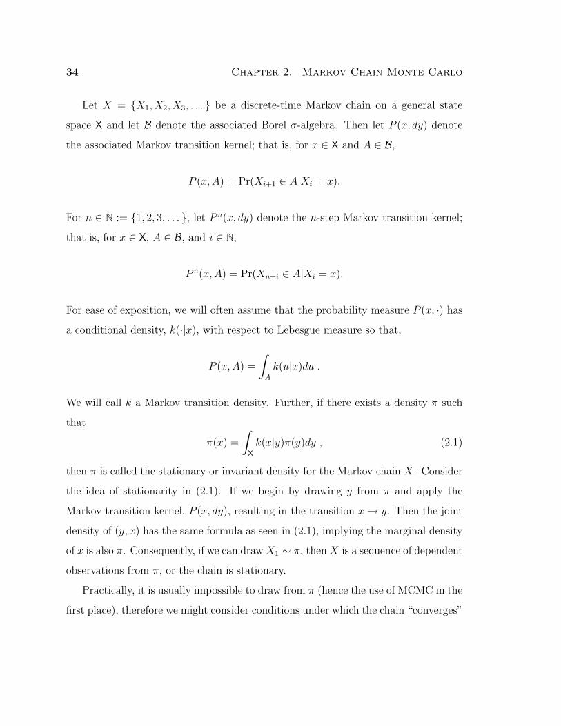
Let X = X1, X2, X3, . . . be a discrete-time Markov chain on a general state
space X and let B denote the associated Borel σ-algebra. Then let P (x, dy) denote
the associated Markov transition kernel; that is, for x ∈ X and A ∈ B,
P (x,A) = Pr(Xi+1 ∈ A|Xi = x).
For n ∈ N := 1, 2, 3, . . . , let P n(x, dy) denote the n-step Markov transition kernel;
that is, for x ∈ X, A ∈ B, and i ∈ N,
P n(x,A) = Pr(Xn+i ∈ A|Xi = x).
For ease of exposition, we will often assume that the probability measure P (x, ·) has
a conditional density, k(·|x), with respect to Lebesgue measure so that,
P (x,A) =
∫A
k(u|x)du .
We will call k a Markov transition density. Further, if there exists a density π such
that
π(x) =
∫X
k(x|y)π(y)dy , (2.1)
then π is called the stationary or invariant density for the Markov chain X. Consider
the idea of stationarity in (2.1). If we begin by drawing y from π and apply the
Markov transition kernel, P (x, dy), resulting in the transition x→ y. Then the joint
density of (y, x) has the same formula as seen in (2.1), implying the marginal density
of x is also π. Consequently, if we can drawX1 ∼ π, thenX is a sequence of dependent
observations from π, or the chain is stationary.
Practically, it is usually impossible to draw from π (hence the use of MCMC in the
first place), therefore we might consider conditions under which the chain “converges”

2.1. Markov Chains 35
to π. Define
‖P n(x, ·)− π(·)‖ := supA∈B
|P n(x,A)− π(A)| ,
the total variation distance between the probability measures P n(x, ·) and π(·). Un-
der regularity assumptions, something can be said about the total variation distance.
First, the following are some important definitions.
Definition 1. A Markov chain transition kernel P is π-irreducible if for any x ∈ X
and for any set A with π(A) > 0, there exists an n such that P n(x,A) > 0.
In other words, starting from any point in the state space, there exists an n such
that there is positive probability we can reach any set having positive π-probability.
If X is a Markov chain with a π-irreducible transition kernel, we will say X is a
π-irreducible Markov chain.
Definition 2. A π-irreducible Markov transition kernel P is periodic if there exists
an integer d ≥ 2 and a collection of disjoint sets A1, . . . , Ad ∈ B such that for each
x ∈ Aj, P (x,Aj+1) = 1 for j = 1, . . . , d − 1, and for each x ∈ Ad, P (x,A1) = 1.
Otherwise, P is said to be aperiodic.
That is, P is periodic if we can partition the state space in such as way as to
introduce cyclic behavior. If no such partition exists, then P is aperiodic. Similarly,
if X is a Markov chain with periodic (aperiodic) P , then we will say X is periodic
(aperiodic).
Definition 3. If X is a π-irreducible Markov chain where π is the stationary distribu-
tion, then X is recurrent if for every set A with π(A) > 0,
Pr(Xn ∈ A i.o.|X1 = x) > 0 for all x ,
Pr(Xn ∈ A i.o.|X1 = x) = 1 for π-almost all x .
The chain is Harris recurrent if Pr(Xn ∈ A i.o.|X1 = x) = 1 for all x.

36 Chapter 2. Markov Chain Monte Carlo
If π is a probability distribution, then X is positive recurrent (or positive
Harris recurrent).
When a chain is π-irreducible, aperiodic, and positive Harris recurrent, we will
call it Harris ergodic.
Proposition 1. Suppose P is π-irreducible and π is an invariant distribution of P .
Then P is positive recurrent and π is the unique invariant distribution of P . If P is
also aperiodic, then, for π-almost all x,
‖P n(x, ·)− π(·)‖ → 0 as n→∞ .
If P is positive Harris recurrent, then the convergence occurs for all x.
Athreya et al. (1996) provide a proof of Proposition 1. The proposition shows the
limit of the total variation norm is zero for Harris ergodic chains, but says nothing
about the rate of convergence. We are particularly interested in bounding the rate
of convergence of the total variation norm because of its connection to Markov chain
CLTs and consistent estimators of the associated asymptotic variance.
The previous chapter defined one rate of convergence which we will use in the
following sections. The formal definition is as follows.
Definition 4. Let X be a Harris ergodic Markov chain with invariant distribution
π. The chain is geometrically ergodic if there exists a constant 0 < t < 1 and a
function M : X 7→ R+ such that for any x ∈ X,
‖P n(x, ·)− π(·)‖ ≤M(x)tn (2.2)
for n ∈ N. If there exists a bounded M satisfying (2.2), then X is uniformly ergodic
(and if X has a finite number of elements, then M is clearly bounded).
2.1. Markov Chains 37
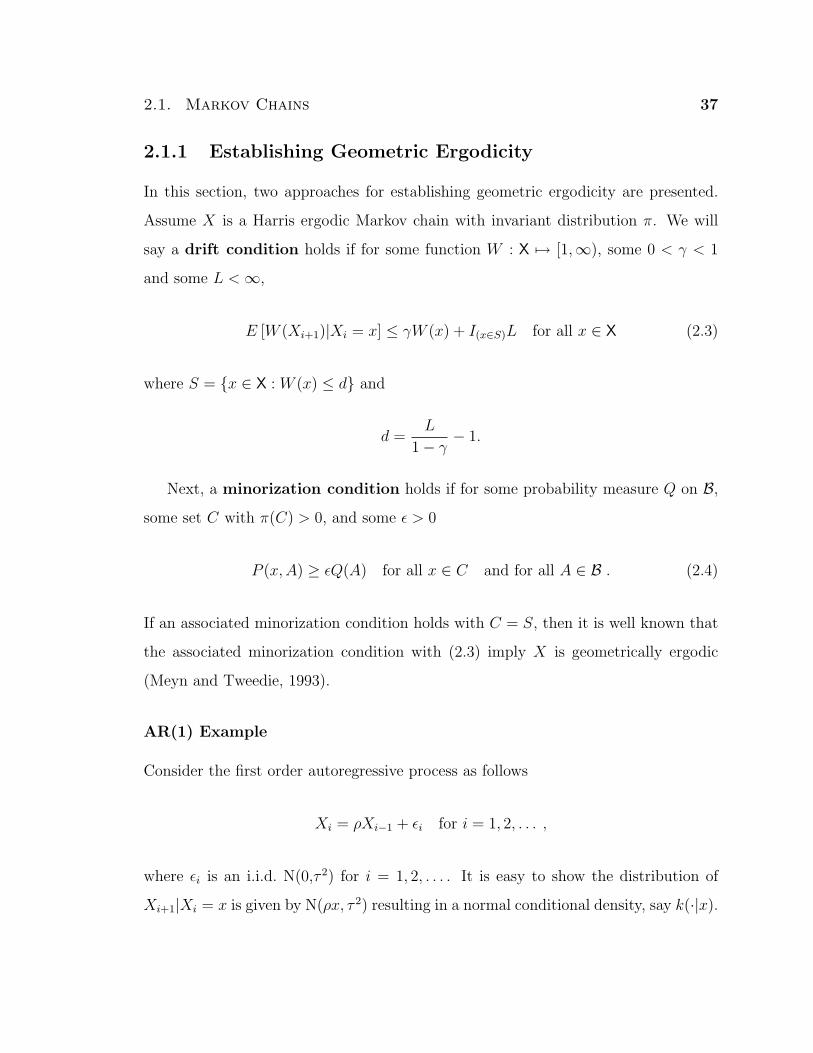
2.1.1 Establishing Geometric Ergodicity
In this section, two approaches for establishing geometric ergodicity are presented.
Assume X is a Harris ergodic Markov chain with invariant distribution π. We will
say a drift condition holds if for some function W : X 7→ [1,∞), some 0 < γ < 1
and some L <∞,
E [W (Xi+1)|Xi = x] ≤ γW (x) + I(x∈S)L for all x ∈ X (2.3)
where S = x ∈ X : W (x) ≤ d and
d =L
1− γ− 1.
Next, a minorization condition holds if for some probability measure Q on B,
some set C with π(C) > 0, and some ε > 0
P (x,A) ≥ εQ(A) for all x ∈ C and for all A ∈ B . (2.4)
If an associated minorization condition holds with C = S, then it is well known that
the associated minorization condition with (2.3) imply X is geometrically ergodic
(Meyn and Tweedie, 1993).
AR(1) Example
Consider the first order autoregressive process as follows
Xi = ρXi−1 + εi for i = 1, 2, . . . ,
where εi is an i.i.d. N(0,τ 2) for i = 1, 2, . . . . It is easy to show the distribution of
Xi+1|Xi = x is given by N(ρx, τ 2) resulting in a normal conditional density, say k(·|x).

38 Chapter 2. Markov Chain Monte Carlo
Let W (x) = x2 + 1, then
E [W (Xi+1)|Xi = x] = ρ2x2 + τ 2 + 1
= ρ2(x2 + 1
)+ τ 2 +
(1− ρ2
)=
1 + ρ2
2W (x)− 1− ρ2
2W (x) + τ 2 +
(1− ρ2
)= γW (x)− (1− γ)W (x) + L ,
where γ := (1 + ρ2)/2 and L := [τ 2 + (1− ρ2)]. Notice, for all x ∈ R
E [W (Xi+1)|Xi = x] ≤ γW (x) + L (2.5)
and if |ρ| < 1 and W (x) > L/ (1− γ)
E [W (Xi+1)|Xi = x] ≤ γW (x) . (2.6)
Combining (2.5) and (2.6) yields
E [W (Xi+1)|Xi = x] ≤ γW (x) + I(x∈S)L for all x ∈ X
where S = x ∈ X : W (x) ≤ dRT and dRT = L/ (1− γ). Further, since
L
1− γ>
L
1− γ− 1
this constitutes a drift condition of the form (2.3).
Next, we will show the associated minorization condition when W (x) ≤ d2. Let
N(µ, τ 2;x) denote the value of the N(µ, τ 2) density at the point x ∈ R. If τ 2 > 0 and

2.1. Markov Chains 39
d ∈ R are fixed, then define h(x)
h(x) := inf−d≤µ≤d
N(µ, τ 2;x
)=
N (d, τ 2;x) if x < 0 ,
N (−d, τ 2;x) if x ≥ 0 .
Then for all x ∈ [−d, d]
k(x|x′) ≥ εq(x)
where ε =∫R h(x)dx and
q(x) =h(x)∫
R h(x)dx.
Thus, the associated minorization condition from (2.4) holds for all x ∈ X with
W (x) ≤ d2 and for all A ∈ B.
Finally, for |ρ| < 1 the AR(1) model is geometrically ergodic.
Rosenthal-type Drift Condition
The drift condition in (2.3) is sometimes referred to as a Roberts-and-Tweedie-type
drift condition (Roberts and Tweedie, 1999, 2001). However, there is an alternative
equivalent drift condition sometimes referred to as a Rosenthal-type drift condition
(Rosenthal, 1995). Again, we will assume X is a Harris ergodic Markov chain with
invariant distribution π. A Rosenthal-type drift condition holds if for some function
V : X 7→ R+, some 0 < λ < 1, and some constant b <∞
E [V (Xi+1)|Xi = x] ≤ λV (x) + b for all x ∈ X . (2.7)
Notice, in (2.7) we are taking the expectation with respect to the Markov transition
kernel. The function V is sometimes called an energy function from the fact when
the drift condition holds, the chain tends to “drift” towards states of lower energy in
terms of expectation.

40 Chapter 2. Markov Chain Monte Carlo
Often, the drift condition in (2.7) can be easier to establish.
Connection Between Drift Functions
Clearly, the drift condition in (2.3) implies the drift condition in (2.7). Jones and
Hobert (2004) show that (2.7) implies (2.3) in general.
Lemma 2. (Jones and Hobert, 2004, Lemma 3.1) Let X be a Harris ergodic Markov
chain with invariant distribution π. Suppose there exists V : X 7→ R+, 0 < λ < 1,
and b <∞ such that
E [V (Xi+1)|Xi = x] ≤ λV (x) + b for all x ∈ X . (2.8)
Set W (x) = 1 + V (x). Then, for any a > 0,
E [W (Xi+1)|Xi = x] ≤ γW (x) + I(x∈S)L for all x ∈ X , (2.9)
where γ = (a+ λ)/(a+ 1), L = b+ (1− λ) and
S =
x ∈ X : W (x) ≤ (a+ 1)L
a(1− γ)
.
Then since(a+ 1)L
a(1− γ)≥ L
(1− γ)− 1 ,
(2.9) constitutes a drift condition of the form of (2.3). Hence, if we can establish
(2.7) and the associated minorization condition
P (x,A) ≥ εQ(A) for all x ∈ X with V (x) ≤ d and for all A ∈ B
then the Markov chain is geometrically ergodic.
2.2. MCMC 41
AR(1) Example
Recall the AR(1) model and let V (x) = x2, then
E [V (Xi+1)|Xi = x] = ρ2x2 + τ 2
= ρ2V (x) + τ 2 ,
for all x ∈ X. Suppose |ρ| < 1, then the drift condition in (2.7) holds where λ ∈ [ρ2, 1)
and b ∈ [τ 2,∞).
An associated minorization condition can be established as before, and hence the
chain is geometrically ergodic if |ρ| < 1.
2.2 Markov Chain Monte Carlo
Suppose that X = X1, X2, X3, . . . is a Harris ergodic Markov chain with state space
X and invariant distribution π (for definitions see Section 2.1). We will maintain these
assumptions throughout this thesis. Typically, estimating Eπg is natural by appealing
to the Ergodic Theorem.
Theorem 1. Let X be a Harris recurrent Markov chain on X with invariant distri-
bution π and g : X → R be a Borel function. If Eπ|g| <∞ then, as n→∞
gn :=1
n
n∑i=1
g(Xi) → Eπg almost surely, (2.10)
for any initial distribution.
This follows directly from Theorems 17.0.1 and 17.1.6 in Meyn and Tweedie
(1993). Applying Theorem 1 to estimate Eπg is easily accomplished by using gn.
MCMC methods entail constructing a Markov chain X satisfying the regularity
conditions described above and then simulating X for a finite number of steps, say
42 Chapter 2. Markov Chain Monte Carlo
n, and using gn to estimate Eπg. The popularity of MCMC methods result from the
ease with which such an X can be simulated (Chen et al., 2000; Robert and Casella,
1999; Liu, 2001).
An obvious question is when should we stop the simulation? That is, how large
should n be? Or, when is gn a good estimate of Eπg? An obvious method of address-
ing the quality of the estimate is to calculate the associated Monte Carlo standard
error of gn. This requires a Central Limit Theorem (CLT), and some stronger reg-
ularity conditions. Specifically, we require the chain to be geometrically ergodic
or uniformly ergodic depending on the moment condition. We will also need to
remember a kernel P satisfies the detailed balance equation with respect to π if
π(dx)P (x, dy) = π(dy)P (y, dx) for all x, y ∈ X . (2.11)
The following states three different sets of regularity conditions (without proof) for
a Markov chain CLT. Other conditions and discussion can be found in Jones (2004)
and Roberts and Rosenthal (2004).
Theorem 2. Let X be a Harris ergodic Markov chain on X with invariant distribution
π, and let g : X → R be a Borel function. Assume one of the following conditions:
1. (Doukhan et al., 1994) X is geometrically ergodic and Eπ [g2(X)(log+|g(X)|)] <
∞;
2. (Roberts and Rosenthal, 1997) X is geometrically ergodic, satisfies (2.11), and
Eπg2(X) <∞; or
3. (Ibragimov and Linnik, 1971) X is uniformly ergodic and Eπg2(X) <∞.
Then, for any initial distribution, as n→∞,
√n(gn − Eπg)
d→ N(0, σ2g) , (2.12)
2.3. Examples 43
where σ2g := varπg(X1)+2
∑∞i=2 covπg(X1), g(Xi); the subscript π means that the
expectations are calculated assuming X1 ∼ π.
Application of Theorem 2 poses two distinct requirements. First, we must ver-
ify the necessary conditions. Specifically, we must ensure the appropriate moment
conditions. We must also construct a Harris ergodic Markov chain, X, with the ap-
propriate invariant distribution π satisfying geometric (or uniform) ergodicity. Once
we have a suitable X, we need to estimate σ2g . This requires specialized techniques
that take into account the dependence in the observed Markov chain. This will be
addressed in Chapter 3.
2.3 Examples
Section 2.1.1 shows the AR(1) model is geometrically ergodic. In future sections,
MCMC will be implemented to estimate EπX. In this case it is easy to show that
EπX = 0 and Eπ |X|d < ∞ for all d < ∞, hence Theorem 2 can be applied. This
section considers a more realistic example.
2.3.1 Hierarchical Linear Mixed Models
Consider the usual frequentist general linear mixed model
Y = Xβ + Zu+ ε ,
where Y is an n× 1 vector of observations, X is a known n× p matrix, Z is a known
n×q matrix, β is a p×1 vector of parameters, u is a q×1 vector of random variables,
and ε is an n× 1 vector of residual errors. We assume that X is of full column rank
so that XTX is invertible. A Bayesian version of this model may be expressed as the
44 Chapter 2. Markov Chain Monte Carlo
following conditionally independent hierarchical model
Y |β, u,R,D ∼ Nn(Xβ + Zu,R−1)
β|u,R,D ∼ Np(β0, B−1)
u|D,R ∼ Nq(0, D−1)
with as yet unspecified priors f(R) and f(D). Here β0 and B−1 are assumed to be
known. The posterior density of (β, u,R,D) given the data, y, is characterized by
π(β, u,R,D|y) ∝ f(y|β, u,R,D)f(β|u,R,D)f(u|D,R)f(R)f(D) . (2.13)
We assume that the priors on R and D are such that the resulting posterior (2.13)
is proper. Even if proper conjugate priors are chosen, the integrals required for
inference through this posterior can not be evaluated in closed form. Thus, exploring
the posterior in order to make inferences might require MCMC.
Block Gibbs Sampler
Consider a block Gibbs sampler with components R, D and ξ = (uT , βT )T . The full
conditional densities for R and D are given by
π(R|ξ,D, y) = C−1R (ξ)|R|1/2 exp−0.5(y −Xβ − Zu)TR(y −Xβ − Zu)f(R)
π(D|ξ, R, y) = C−1D (ξ)|D|1/2 exp−0.5uTDuf(D)
where | · | is a determinant,
CR(ξ) =
∫|R|1/2 exp−0.5(y −Xβ − Zu)TR(y −Xβ − Zu)f(R) dR ,
2.3. Examples 45
and
CD(ξ) =
∫|D|1/2 exp−0.5uTDuf(D) dD .
The density π(ξ|R,D, y) is (p+q)–variate Normal with mean ξ0 and covariance matrix
Σ−1 where
Σ =
ZTRZ +D ZTRX
XTRZ XTRX +B
and Σξ0 =
ZTRy
XTRy +Bβ0
. (2.14)
Consider the block Gibbs sampler corresponding to the following updating scheme:
(D′, R′, ξ′) → (D,R′, ξ′) → (D,R, ξ′) → (D,R, ξ) .
Conditional on ξ, D and R are independent and hence the order in which they are
updated is irrelevant. That is, we are effectively dealing with a two-variable Gibbs
sampler. Suppressing dependence on the data, the transition density is given by
k(D,R, ξ|D′, R′, ξ′) = π(D|ξ′)π(R|ξ′)π(ξ|R,D) .
A Special Case
In this section, we identify a specific example of the model in Section 2.3.1 and
establish drift and minorization conditions for the block Gibbs sampler. Johnson and
Jones (2008) consider a much broader class of models. Suppose that p = 1 so that
X = (x1, . . . , xn)T ∈ Rn and that q = n with Z = In. Fix β0 = 0 and B−1 = 1.
Assume that R−1 = λ−1R In and D−1 = λ−1
D In where λ−1R and λ−1
D are scalar variance
components whose reciprocals are assigned the following conjugate priors
λR ∼ Gamma(r1, r2) and λD ∼ Gamma(d1, d2) .

46 Chapter 2. Markov Chain Monte Carlo
Set ξ = (uT , β)T and λ = (λD, λR)T .
Recall that the block Gibbs sampler from the previous section uses the sampling
scheme: (λ′, ξ′) → (λ, ξ′) → (λ, ξ). The full conditionals for the precision parameters
are given by
λR|ξ, y ∼ Gamma
(r1 +
n
2, r2 +
1
2(y −Xβ − u)T (y −Xβ − u)
),
λD|ξ, y ∼ Gamma
(d1 +
n
2, d2 +
1
2uTu
).
Let P be the transition kernel of this Gibbs sampler. Now ξ|λR, λD, y ∼ Nn+1(ξ0,Σ−1)
where
Σ =
(λR + λD)In λRX
λRXT 1 + λRX
TX
and Σξ0 = λR
y
XTy
. (2.15)
We establish the drift condition for this sampler in Section 2.4.3 and the associated
minorization condition in Section 2.4.3. From these, we can conclude the chain is
geometrically ergodic (see Section 2.1.1 for details).
2.4 Proofs and Calculations
2.4.1 Proof of Lemma 2
This proof is shown in Jones and Hobert (2004). Clearly, (2.8) implies that
E [W (Xi+1)|Xi = x] ≤ λW (x) + b+ (1− λ) = λW (x) + L for all x ∈ X .
Set ∆W (x) = E [W (Xi+1)|Xi = x]−W (x) and β = (1− λ)/(a+ 1). Then
E [W (Xi+1)|Xi = x] ≤ [1− (a+ 1)β]W (x) + L
2.4. Proofs and Calculations 47
or, equivalently,
∆W (x) ≤ −βW (x)− aβW (x) + L for all x ∈ X .
If x /∈ C, then
W (x) >(a+ 1)L
a(1− γ)>
(a+ 1)L
a(1− λ)=
L
aβ.
Now write W (x) = Laβ
+ s(x), where s(x) > 0. Then
∆W (x) ≤ −βW (x)− aβ
[L
aβ+ s(x)
]+ L
= −βW (x)− aβs(x)
≤ −βW (x) .
If, on the other hand, x ∈ C, then
∆W (x) ≤ −βW (x)− aβW (x) + L
≤ −βW (x) + L .
Now putting these together gives
E [W (Xi+1)|Xi = x] ≤ (1− β)W (x) + I(x∈S)L
= γW (x) + I(x∈S)L .
2.4.2 Mixing Conditions
This section will provide connections between different mixing conditions for future
use. Specifically, the goal of this section is to show that geometrically ergodic Markov
chains are exponentially fast alpha-mixing. We begin by deriving the coupling in-

48 Chapter 2. Markov Chain Monte Carlo
equality.
Let X = X1, X2, X3, . . . and Y = Y1, Y2, Y3, . . . be two Markov chains with
common transition kernel P satisfying the minorization condition in (2.4). Suppose
X1 is an arbitrary starting point in X and Y1 ∼ π, hence Y is stationary.
Then for each x ∈ C, define the residual kernel as
R(x, dy) =P (x, dy)− εQ(dy)
1− εfor ε < 1 ,
and R(x, ·) := 0 for ε = 1. It is easy to verify R is a transition kernel, and that
P (x, dy) = εQ(dy) + (1− ε)R(x, dy) .
Using this representation, we can consider updating X and Y in the following manner.
Let Xn = x and Yn = y.
1. If x = y, generate Z ∼ P (x, ·), and set Xn+1 = Yn+1 = Z.
2. If x 6= y, x ∈ C, and y ∈ C, generate δ ∼ Bernoulli(ε) then
(a) if δ = 0, generate Xn+1 ∼ R(x, ·) and Yn+1 ∼ R(y, ·) independently;
(b) if δ = 1, generate Z ∼ Q(·) and set Xn+1 = Yn+1 = Z.
3. If x 6= y and x /∈ C or y /∈ C generate Xn+1 ∼ P (x, ·) and Yn+1 ∼ P (y, ·)
independently.
It is clear this method retains the original transition kernel P for both chains. It is
also clear that if Xn = Yn, then Xn+k = Yn+k for all k ∈ N. In other words, once
the chains have coupled, all future draws of the two chains remain equal. Define
the coupling time as T = inf t : Xt = Yt, the random time when the two chains
couple.

2.4. Proofs and Calculations 49
The following is the classical derivation of the coupling inequality
|P n(x0, A)− π(A)| = |Pr(Xn ∈ A)− Pr(Yn ∈ A)|
= |Pr(Xn ∈ A,Xn = Yn) + Pr(Xn ∈ A,Xn 6= Yn)−
Pr(Yn ∈ A,Xn = Yn)− Pr(Yn ∈ A,Xn 6= Yn)|
= |Pr(Xn ∈ A,Xn 6= Yn)− Pr(Yn ∈ A,Xn 6= Yn)|
≤ max Pr(Xn ∈ A,Xn 6= Yn),Pr(Yn ∈ A,Xn 6= Yn)
≤ Pr(Xn 6= Yn) ≤ Pr(T > n) .
Resulting in the coupling inequality
‖P n(x, ·)− π(·)‖ ≤ Pr(T > n) . (2.16)
Under our assumptions (Jones, 2004), the coupling time is almost surely finite and
Pr(T > n) → 0 as n→∞.
We will use the coupling inequality to show that Harris ergodic Markov chains
satisfying (2.4) are alpha mixing. First, let Fmk = σ(Xk, . . . , Xm).
Definition 5. The sequence X is said to be alpha-mixing (or strongly mixing) if
α(n) → 0 as n→∞ where
α(n) := supk≥1
supA∈Fk
1 ,B∈F∞k+n
|P(A ∩B)− P(A)P(B)| .
Then let A and B be Borel sets so that by (2.16)
|P n(x,A)− π(A)| ≤ Prx(T > n)
50 Chapter 2. Markov Chain Monte Carlo
and
∫B
Prx(T > n)π(dx) ≥∫
B
|P n(x,A)− π(A)|π(dx)
≥ |∫
B
[P n(x,A)− π(A)]π(dx)|
= |Pr(Xn ∈ A and X1 ∈ B)− π(A)π(B)| .
Then α(n) ≤ Eπ [Prx(T > n)] and a dominated convergence argument shows that
Eπ [Prx(T > n)] → 0 as n→∞ ,
and hence α(n) → 0 as n→∞.
Similarly, consider a geometrically ergodic Markov chain satisfying (2.2). Using
the same argument, let A and B be Borel sets so
|P n(x,A)− π(A)| ≤M(x)tn
and
∫B
M(x)tnπ(dx) ≥∫
B
|P n(x,A)− π(A)|π(dx)
≥ |∫
B
[P n(x,A)− π(A)]π(dx)|
= |Pr(Xn ∈ A and X1 ∈ B)− π(A)π(B)| .
Then α(n) ≤ tnEπM(x) and if EπM(x) <∞, α(n) → 0 as n→∞.
Following the argument from Jones (2004), we want to show EπM(x) <∞. First,
notice that from either drift condition (2.7) or (2.3), we can take M(x) ∝ W (x) in
(2.2). Then we can appeal to Theorem 14.3.7 in Meyn and Tweedie (1993) that shows
if (2.3) holds then EπW (x) < ∞. Since a geometrically ergodic chain is equivalent

2.4. Proofs and Calculations 51
to (2.3) (Meyn and Tweedie, 1993, Chapter 16) we can conclude that geometrically
ergodic Markov chains satisfy (2.2) with EπM(x) <∞. In other words, geometrically
ergodic Markov chains are exponentially fast alpha-mixing.
Remark 1. Results for a Markov chain CLT for quantiles require∑∞
i=1 α(i) < ∞
(Chapter 4). If X is a geometrically ergodic Markov chain, then
∞∑i=1
α(i) ≤∞∑i=1
ti [EπM(x)]
= [EπM(x)]1
1− t<∞ ,
because 0 < t < 1.
2.4.3 Block Gibbs Sampler
To simulate from this multivariate normal distribution we require the Cholesky de-
composition of Σ in (2.15), Σ = LLT , where L is
L =
l1 0
l2 l3
.
Solving for L we obtain
l1 = aIn, l2 = bXT , and l3 = c
where a =√λR + λD , b = λR/a and c =
√1 + (λRλD/a2)XTX. It is easy to see
that
L−1 =
a−1In 0
−b(ac)−1XT c−1
,

52 Chapter 2. Markov Chain Monte Carlo
and hence
Σ−1 =
a−2In + (b/ac)2XXT −b/ac2X
−b/ac2XT c−2
=
1λR+λD
[In +
λ2R
λR+λD+λRλDXT XXXT
]−λR
λR+λD+λRλDXT XX
−λR
λR+λD+λRλDXT XXT λR+λD
λR+λD+λRλDXT X
.
Also,
ξ0 =
λR
λR+λDY − λ2
RλD
(λR+λD)(λR+λD+λRλDXT X)XXTY
λRλD
λR+λD+λRλDXT XXTY
.
It is now easy to obtain the following expectations that we will require later.
E(λD|ξ) =2d1 + n
2d2 + uTu
E(λ−1D |ξ) =
2d2 + uTu
2d1 + n− 2
E(λR|ξ) =2r1 + n
2r2 + (Y −Xβ − u)T (Y −Xβ − u)
E(λ−1R |ξ) =
2r2 + (Y −Xβ − u)T (Y −Xβ − u)
2r1 + n− 2
E(β|λ) =λRλD
λR + λD + λRλDXTXXTY
E(ui|λ) =λR
λR + λD
[yi − xiE(β|λ)]
Var(β|λ) =λR + λD
λR + λD + λRλDXTX
Var(ui|λ) =1
λR + λD
[1 +
λ2Rx
2i
λR + λD + λRλDXTX
]Cov(β, ui|λ) =
−λRxi
λR + λD + λRλDXTX
Cov(ui, uj|λ) =λ2
Rxixj
(λR + λD)(λR + λD + λRλDXTX), i 6= j .

2.4. Proofs and Calculations 53
Now
yi − xiE(β|λ) = yi − xiλRλD
λR + λD + λRλDXTXXTY
=(λR + λD)yi + λRλDX
TX(yi − xiXTY/XTX)
λR + λD + λRλDXTX,
and hence yi − xiE(β|λ) is a convex combination of yi and yi − xiXTY/XTX. Let ∆
denote the convex hull of the set
(yi, yi − xiX
TY/XTX)
for i = 1, . . . , n.
Then
yi − xiE(β|λ)− E(ui|λ) =λD
λR + λD
[yi − xiE(β|λ)]
and hence
[yi − xiE(β|λ)− E(ui|λ)]2 ≤ ∆2 .
Drift for the Block Gibbs Sampler
In this section, we develop a drift condition as in (2.7) for the block Gibbs sampler.
Set
V1(ξ) = (Y −Xβ − u)T (Y −Xβ − u)
and V2(u) = uTu. These will be used in establishing both the drift and minorization
conditions.
Theorem 3. Suppose r1 > 1 and d1 > 1 and fix
γ ∈(
max
n
2r1 + n− 2,
n
2d1 + n− 2
, 1
).
54 Chapter 2. Markov Chain Monte Carlo
Define V (ξ) = φ1V1(ξ) + φ2V2(ξ). Then for any positive φ1 and φ2
PV (ξ′) ≤ γV (ξ′) + b
where PV (ξ′) = E[V (ξ)|λ′, ξ′] and
b =nφ1∆2 + φ1X
TX + 2φ1r2n
2r1 + n− 2
+nφ2∆2 + φ2X
TX + 2φ2d2(n+ 1)
2d1 + n− 2.
Proof. Notice
E(V (ξ)|λ′, ξ′) = φ1E(V1(ξ)|ξ′) + φ2E(V2(ξ)|ξ′) .
The required expectations will be calculated separately via the following rule:
E[Vi(ξ)|λ′, ξ′] = E[Vi(ξ)|ξ′] = E[E(Vi(ξ)|λ)|ξ′] ,
for i = 1, 2.
First consider the inner expectation in E[E(V1(ξ)|λ)|ξ′].
E(V1(ξ)|λ) =n∑
i=1
E[(yi − xiβ − ui)2|λ]
=n∑
i=1
Var[(yi − xiβ − ui)|λ] + [E(yi − xiβ − ui)|λ]2
=n∑
i=1
x2i Var(β|λ) + Var(ui|λ) + 2xiCov(β, ui|λ)
+ [yi − xiE(β|λ)− E(ui|λ)]2

2.4. Proofs and Calculations 55
and hence
E(V1(ξ)|λ) ≤n∑
i=1
x2i Var(β|λ) + Var(ui|λ) + 2xiCov(β, ui|λ) + n∆2
=n
λR + λD
+(λR + λD)2 + λ2
R − 2λR(λR + λD)
(λR + λD)(λR + λD + λRλDXTX)XTX + n∆2
=n
λR + λD
+λ2
D
(λR + λD)(λR + λD + λRλDXTX)XTX + n∆2
≤ n
λR
+
(λD
λR + λD + λRλDXTX
)XTX + n∆2
≤ n
λR
+λD
λD
XTX + n∆2
=n
λR
+XTX + n∆2 .
Now for the outer expectation.
E(V1(ξ)|ξ′) ≤ nE(λ−1R |ξ′) +XTX + n∆2
= n2r2 + (Y −Xβ′ − u′)T (Y −Xβ′ − u′)
2r1 + n− 2+XTX + n∆2
=n
2r1 + n− 2V1(ξ
′) +2r2n
2r1 + n− 2+XTX + n∆2 .
Now consider calculating E[E(V2(ξ)|λ)|ξ′]. We will again consider the inner expecta-
tion first.
E(V2(u)|λ) =n∑
i=1
Var(ui|λ) + [E(ui|λ)]2
=n
λR + λD
+λ2
R
(λR + λD)(λR + λD + λRλDXTX)XTX
+
(λR
λR + λD
)2
n∆2
≤ n
λD
+
(λR
λR + λD
)(λR
λR + λD + λRλDXTX
)XTX + n∆2
≤ n
λD
+XTX + n∆2 .

56 Chapter 2. Markov Chain Monte Carlo
Hence
E(V2(u)|ξ′) ≤ nE(λ−1D |ξ′) +XTX + n∆2
=n
2d1 + n− 2V2(u
′) +2d2n
2d1 + n− 2+XTX + n∆2 .
Combining these two calculations yields
PV (ξ′) ≤ φ1
[n
2r1 + n− 2V1(ξ
′)
]+ φ2
[n
2d1 + n− 2V2(u
′)
]+ b
≤ γV (ξ′) + b .
Minorization for the Block Gibbs Sampler
In this section, we develop a minorization condition of the form (2.4) for the block
Gibbs sampler by closely following the argument of Jones and Hobert (2004). We
wish to establish the minorization condition on the set
SB = ξ : V (ξ) ≤ dR = ξ : φ1V1(ξ) + φ2V2(ξ) ≤ dR ,
for any dR > 0. First note that SB is contained in CB := CB1 ∩ CB2 , where
CB1 = ξ : V1(ξ) ≤ dR/φ1 and CB2 = ξ : V2(ξ) ≤ dR/φ2 .
Hence, it suffices to establish a minorization condition that holds on CB. This will
require the following lemma.
Lemma 3. (Jones and Hobert, 2004, Lemma 4.1) Let Gamma(α, β;x) denote the
value of the Gamma(α, β) density at the point x > 0. If α > 1, b > 0, and c > 0 are

2.4. Proofs and Calculations 57
fixed, then, as a function of x
inf0<β<c
Gamma(α, b+ β/2;x) =
Gamma(α, b;x) if x < x∗ ,
Gamma(α, b+ c/2;x) if x > x∗ ,
where
x∗ =2α
clog(1 +
c
2b
).
We now present the minorization condition for the block Gibbs sampler.
Theorem 4. Let q(λ, ξ) be a density on R2+ × Rn+1 such that
q(λ, ξ) =
[h1(λR)∫
R+h1(λR)dλR
][h2(λD)∫
R+h2(λD)dλD
]π(ξ|λ, y),
where
h1(λR) =
Gamma(r1 + n
2, r2;λR
)if λR < λ∗R
Gamma(r1 + n
2, r2 + dR
2φ1;λR
)if λR ≥ λ∗R
for
λ∗R =φ1(2r1 + n)
dR
log
(1 +
dR
2φ1r2
)and
h2(λD) =
Gamma(d1 + n
2, d2;λD
)if λD < λ∗D
Gamma(d1 + n
2, d2 + dR
2φ2;λD
)if λD ≥ λ∗D
for
λ∗D =φ2(2d1 + n)
dR
log
(1 +
dR
2φ2d2
).
Then the following minorization condition is satisfied for the Markov transition den-
sity of the block Gibbs sampler:
k(λ, ξ|λ′, ξ′) ≥ εq(λ, ξ) for all ξ′ ∈ CB

58 Chapter 2. Markov Chain Monte Carlo
where ε =[∫
R+h1(λR)dλR
] [∫R+h2(λD)dλD
].
Proof. Assume ξ′ ∈ CB and recall that
π(λR|ξ′) = Gamma(r1 + n/2, r2 + V1(ξ′)/2;λR) ,
π(λD|ξ′) = Gamma(d1 + n/2, d2 + V2(ξ′)/2;λD) .
Therefore,
k(λ, ξ|λ′, ξ′) = π(λR|ξ′, y)π(λD|ξ′, y)π(ξ|λ, y)
≥ π(ξ|λ, y) infξ′∈CB1
∩CB2
[π(λR|ξ′, y)π(λD|ξ′, y)]
≥ π(ξ|λ, y)[
infξ′∈CB1
∩CB2
π(λR|ξ′, y)] [
infξ′∈CB1
∩CB2
π(λD|ξ′, y)]
≥ π(ξ|λ, y)[
infξ′∈CB1
π(λR|ξ′, y)] [
infξ′∈CB2
π(λD|ξ′, y)]
where
infξ′∈CB1
π(λR|ξ′, y) = infξ′:v1(ξ′)≤dR/φ1
π(λR|ξ′, y) = h1(λR)
and
infξ′∈CB2
π(λD|ξ′, y) = infξ′:v2(ξ′)≤dR/φ2
π(λD|ξ′, y) = h2(λD).
This gives us k(λ, ξ|λ′, ξ′) ≥ q(λ, ξ) for
q(λ, ξ) ∝ π(ξ|λ)h1(λR)h2(λD).

Chapter 3
Monte Carlo Error
As we have seen, MCMC is a common statistical method where the goal is esti-
mating characteristics of a target distribution. An important, and often overlooked,
secondary goal is estimation of the associated asymptotic variance in the Markov
chain central limit theorem. Specifically, the variance is required in evaluating the
Monte Carlo standard error (MCSE) which is useful in measuring the accuracy of
the resulting estimate. We introduce several techniques for estimating the variance:
batch means, overlapping batch means, regeneration and spectral variance estimation.
In addition, we establish conditions under which these methods produce strongly
consistent estimators. For batch means and overlapping batch means, we establish
conditions which ensure consistency in the mean-square sense. Using mean-square
consistency, we calculate “optimal” batch sizes that minimize the asymptotic mean-
square error. Finally, we examine the finite sample properties in the context of some
examples and provide recommendations for practitioners.
Some of this chapter is contained in Flegal and Jones (2008). The results here are
expanded to contain the relevant supporting material from the literature.
59
60 Chapter 3. Monte Carlo Error
3.1 Introduction
Suppose the goal is to calculate Eπg :=∫
Xg(x)π(dx) where g is a real-valued, π-
integrable function on X and π is a probability distribution with support X. Let
X = X1, X2, X3, . . . be a Harris ergodic Markov chain on a general space X having
invariant distribution π. The Ergodic Theorem from Chapter 2 shows with probability
one,
gn := n−1
n∑i=1
g(Xi) → Eπg as n→∞ . (3.1)
Clearly, the resulting Monte Carlo approximation will not be exact. In other words,
we would rarely expect our estimate, gn, to equal the true quantity of interest, Eπg.
The estimate is bound to be off by some amount, gn − Eπg, previously defined as
the Monte Carlo error. Unless Eπg is known, we will never know the true Monte
Carlo error. However, we can assess this error by estimating the variance from the
asymptotic distribution of gn.
More specifically, suppose a Markov chain central limit theorem (CLT) exists for
g, for any initial distribution,
√n(gn − Eπg)
d→ N(0, σ2g) as n→∞ (3.2)
where σ2g := varπg(X1) + 2
∑∞i=2 covπg(X1), g(Xi). The issue we study here is
how to consistently estimate σ2g .
3.1.1 Stopping the Simulation
Estimating σ2g is an important issue in MCMC output analysis since the estimate can
be used to decide when to terminate the simulation or assess the reliability of the
current point estimate gn; see Flegal et al. (2008), Hobert et al. (2002) and Jones
et al. (2006).
3.1. Introduction 61
When choosing a stopping criteria for MCMC simulations, a practitioner is forced
to choose between one long run or several independent smaller runs. Using one long
run requires specialized techniques which incorporate the dependent nature of the
underlying Markov chain. In contrast, the use of multiple Markov chains (i.e. the
Gelman-Rubin Diagnostic from Chapter 1) uses independent chains but each chain
may be too short to overcome the initial bias. Alexopoulos and Goldsman (2004)
investigate this issue for general processes and conclude that one long run is preferable
for nonstationary processes. With this in mind, we will focus on these techniques,
but further investigation may be warrented for geometrically (or uniformly) ergodic
Markov chains.
A number of other stopping criteria have been proposed based on convergence
diagnostics (Cowles and Carlin, 1996). However, convergence diagnostics have done
little other than confuse practitioners; see Flegal et al. (2008) and Jones et al. (2006).
In general, diagnostics simply ignore the appropriate problem of accurately estimating
σ2g , and hence we ignore them in this discussion.
Instead, we will focus on two main approaches to stopping an MCMC simulation,
fixed-length methods and fixed-width methods.
Fixed-Length Approach
The simplest approach to stopping an MCMC simulation is to run a single chain for
a fixed number of iterations then use gn to estimate Eπg. Practitioners using this
approach should report the resulting MCSE to allow the reader to infer the accuracy
of the estimate. Hence, estimating σ2g is required. Suppose we can construct an
estimator, say σ2n, such that σ2
n is mean-square consistent, or as n→∞
MSE(σ2n) := Eπ(σ2 − σ2
g)2 → 0 . (3.3)

62 Chapter 3. Monte Carlo Error
Damerdji (1995) establishes (3.3) for general stationary processes. Section 3.2.3 spe-
cializes this work to MCMC and addresses errors from Damerdji (1995).
Given potential estimators of σ2g , we can use (3.3) to choose nuisance parameters
to minimize the asymptotic mean-square error (MSE). Song and Schmeiser (1995)
propose one such approach to batch size selection for general stationary processes;
Section 3.2.3 considers this in the context of MCMC.
Fixed-Width Methods
Suppose we have an idea of the level of accuracy we want in our estimate, gn. For
example, suppose we want to report estimates with three significant figures. One way
of achieving this goal is through evaluation of the Monte Carlo error.
Assessing the Monte Carlo error is usually accomplished by appealing to a Markov
chain CLT (Theorem 2). Then one can calculate an estimate of the MCSE of gn, say
σn/√n and form a confidence interval for Eπg. If this interval is too large, then the
value of n is increased and simulation continues until the interval is sufficiently small.
The half-width of the interval is given by
t∗σn√n< ε (3.4)
where t∗ is an appropriate quantile and ε > 0 is the user-specified half-width.
Not knowing ahead of time the number of iterations necessary to ensure the desired
precision, the method requires a sequential approach where the chain will be run for
a random number of iterations. The theoretical justification of this method requires
a strongly consistent estimator of σ2g . Specifically, an estimator is strongly consistent
if with probability one,
σ2n → σ2
g as n→∞ . (3.5)
We can use σ2n to form an asymptotically valid confidence interval for Eπg or use it to
3.2. Variance Estimation 63
implement the fixed-width methods for stopping the simulation introduced in Glynn
and Whitt (1992) for general processes and in MCMC by Jones et al. (2006).
Remark 2. In general, both (3.3) and (3.5) imply convergence in probability, but
mean-square consistency and strong consistency do not in general imply one another.
3.2 Variance Estimation
Estimating σ2g in (3.2) requires specialized techniques that take into account the
dependence in the observed Markov chain. Many methods have been proposed to
estimate σ2g , including non-overlapping batch means (BM), overlapping batch means
(OBM), spectral variance methods (SV), and regenerative simulation (RS); see Fish-
man (1996) for an overview. These methods all have advantages and disadvantages.
For example, RS will produce an estimator satisfying (3.5) under the conditions guar-
anteeing (3.2), however, implementing RS typically requires additional theoretical
work. Some common ways of implementing BM and OBM lead to estimators that
are demonstrably not consistent (Glynn and Iglehart, 1990; Glynn and Whitt, 1991)
thus some authors encourage caution in their use; see Roberts (1996). On the other
hand, both BM and OBM are simple to implement but OBM has the reputation for
being more efficient that BM. SV methods are also easy to implement, however they
have received limited attention in MCMC settings.
In our theoretical work, we focus on conditions which guarantee (3.5) for SV and
OBM estimators. These estimators are closely connected since it is well known (An-
derson, 1984; Meketon and Schmeiser, 1984) that OBM is, aside from the end-effect
terms, equal to a spectral variance estimator with the modified Bartlett lag window.
This has also been addressed by Damerdji (1994) but our regularity conditions are
weaker. Further, in BM and OBM, batch size selection is still an open research
problem. Song and Schmeiser (1995) propose an approach that minimizes the mean-
64 Chapter 3. Monte Carlo Error
squared error in (3.3) with a certain rate of convergence. We will show the estimators
of σ2g using BM and OBM are mean-square consistent. Under additional conditions,
we show the “optimal” batch size in terms of MSE is proportional to n1/3. However,
we will show that it is impractical to use this result in finite sample settings.
3.2.1 Notation and Assumptions
Throughout this thesis, the symbol “O” will represent the usual big-O notation and
the symbol “o” will represent the usual little-o notation. Suppose f(n) and g(n) are
functions defined on R. Formally, if f(n) = O (g(n)), then there exists an n0 and
M > 0 such that |f(n)| ≤ M |g(n)| for all n > n0. Further, if f(n) = o (g(n)), then
for any M > 0 there exists an n0 such that |f(n)| < M |g(n)| for all n > n0.
Either geometric or uniform ergodicity along with a moment condition on g will
ensure a Markov chain CLT in (3.2) (Jones, 2004; Roberts and Rosenthal, 2004). How-
ever, throughout this discussion we will require a different asymptotic property, specif-
ically a strong invariance principle which is now described. Let B = B(t), t ≥ 0
denote a standard Brownian motion. A strong invariance principle holds if there
exists a nonnegative increasing function ψ(n) on the positive integers, a constant
0 < σg <∞, and a sufficiently rich probability space such that∣∣∣∣∣n∑
i=1
g(Xi)− nEπg − σgB(n)
∣∣∣∣∣ = O(ψ(n)) w.p.1 as n→∞ (3.6)
where the w.p.1 in (3.6) means for almost all sample paths ω ∈ Ω. Alternatively,
(3.6) can be expressed as there exists n0 and a finite random variable C such that for
almost all sample paths ω ∈ Ω of the process,∣∣∣∣∣n∑
i=1
Yi − nEπg − σgB(n)
∣∣∣∣∣ < C(ω)ψ(n) (3.7)
3.2. Variance Estimation 65
for all n > n0. A strong invariance principle is enough to guarantee both (3.1) and
(3.2) among other properties; see Philipp and Stout (1975) and Damerdji (1991). Of
course, directly establishing a strong invariance principle may be difficult in practice.
We will rely on the following result first established by Jones et al. (2006) and later
extended by Bednorz and Latuszynski (2007).
Lemma 4. Let g : X 7→ R be a Borel function and let X be a Harris ergodic Markov
chain with invariant distribution π.
1. If X is uniformly ergodic and Eπ|g|2+δ′ < ∞ for some δ′ > 0, then (3.6) holds
with ψ(n) = n1/2−α′ where α′ ≤ δ′/(24 + 12δ′).
2. If X is geometrically ergodic and Eπ|g|2+δ+ε < ∞ for some δ > 0 and some
ε > 0, then (3.6) holds with ψ(n) = nα log n where α = 1/(2 + δ).
3.2.2 Spectral Density Estimation
In this section, we investigate conditions which guarantee strong consistency, i.e.
(3.5), of spectral variance estimators. For a detailed review of spectral analysis in a
time–series context see Anderson (1994) and Priestley (1981).
Define the process Y = Yi = g(Xi) − Eπg for i = 1, 2, 3, . . . and Yj(k) :=
k−1∑k
i=1 Yj+i for j = 0, . . . , n − bn and k = 1, . . . , bn. Further define Yn := Y1(n) =
n−1∑n
i=1 Yi. First note that
σ2g =
∞∑s=−∞
γ(s)
where γ(s) := Eπ [YtYt+s] = Eπ [(g(Xt)− Eπg)(g(Xt+s)− Eπg)]. This representation
is similar to the spectral density function, or the Fourier transform of the covariance
sequence,
f(φ) =1
2π
∞∑s=−∞
γ(s) cos(φs)

66 Chapter 3. Monte Carlo Error
where the parameter φ is the frequency.
Remark 3. General time-series settings may require additional work to establish the
existence of f(φ). Given a Markov chain CLT this quantity is certain to exist and be
finite.
First consider estimating γ(s) using the sample analog of the covariance of lag
s ≥ 0,
γn(s) = n−1
n−s∑t=1
(Yt − Yn)(Yt+s − Yn) . (3.8)
If Eπg2 <∞, then we can appeal to the Ergodic Theorem to show that γn(s) → γ(s)
almost surely for each fixed s as n → ∞. One could then use the sample analog in
(3.8) to estimate f(φ), though this turns out to be a poor estimator (see Anderson,
1994; Bratley et al., 1987). Instead, we will introduce the use of a weight function,
wn(·), commonly called the lag window in the literature. We will restrict our attention
to lag windows fulfilling the following requirements.
Assumption 1. The lag window wn(·) is an even function defined on Z such that
|wn(s)| ≤ 1 for all n and s,
wn(0) = 1 for all n,
wn(s) = 0 for all |s| ≥ bn ,
where bn is the truncation point.
We will also require the following assumption on the truncation point.
Assumption 2. Let bn be an integer sequence such that bn → ∞ and n/bn → ∞ as
n→∞ where bn and n/bn are monotonically nondecreasing.

3.2. Variance Estimation 67
Note 2πf(0) =∑∞
−∞ γ(s) = σ2g which can be estimated with
2πfn(0) =bn−1∑
s=−(bn−1)
wn(s)γn(s) . (3.9)
The main result of this section follows.
Theorem 5. Let X be a geometrically ergodic Markov chain with invariant dis-
tribution π and g : X → R be a Borel function with Eπ|g|2+δ+ε < ∞ for some
δ > 0 and ε > 0. Suppose Assumptions 1 and 2 hold and define ∆1wn(k) =
wn(k − 1)−wn(k) and ∆2wn(k) = wn(k − 1)− 2wn(k) +wn(k + 1). Further suppose
(a) bnn−1∑bn
k=1 k |∆1wn(k)| → 0 as n → ∞; (b) there exists a constant c ≥ 1 such
that∑
n(bn/n)c < ∞; (c) b−1n log n stays bounded as n → ∞; (d) bnn
−1 log n → 0 as
n→∞; (e)
bnn2α(log n)3
(bn∑
k=1
|∆2wn(k)|
)2
→ 0 as n→∞, and
n2α(log n)2
bn∑k=1
|∆2wn(k)| → 0 as n→∞
where α = 1/(2 + δ); and (f) b−1n n2α log n→ 0 as n→∞. Then
2πfn(0) → σ2g as n→∞ w.p.1.
Proof. Consider the following quantity,
σ2(n) = n−1
n−bn∑j=0
bn∑k=1
αn(k)(Yj(k)− Yn
)2(3.10)
where αn(k) is a sequence of weights. Proposition 3 in Section 3.4.2 shows there exists
a sequence of weights αn(k) := k2∆2wn(k) and a sequence dn due to some end effects,
68 Chapter 3. Monte Carlo Error
such that
σ2(n) = 2πfn(0)− dn .
Proposition 7 in Appendix A.1.1 shows σ2∗ → 1 as n→∞ where σ2
∗ is the Brownian
motion equivalent of (3.10). Lemma 4 with Lemma 8 show σ2(n) − σ2g σ
2∗ → 0 as
n → ∞. Finally, Lemma 9 with Lemma 10 shows that dn → 0 as n → ∞. Thus,
combining all of these yields the desired result.
Remark 4. It is convenient in applications to take bn = bnνc for some 0 < ν < 1, and
hence (b), (c), and (d) are satisfied.
Lag Windows
Anderson (1994) gives an extensive collection of lag windows satisfying Assumption 1.
In this section, we discuss some of the more popular windows.
The Parzen lag windows, wn(k) = 1− |k|q/bqn for |k| < bn and 0 otherwise where
q > 0. For this type of window, (a) of Theorem 5 reduces to b2nn−1 → 0 as n→∞ and
(e) requires b1−2qn n2α(log n)3 → 0 and b−q
n n2α(log n)2 → 0 as n → ∞. The modified
Bartlett lag window is a special case of a Parzen window where q = 1, hence the
result applies.
The Tukey-Hanning window, wn(k) = [1 + cos(πk/bn)] /2 for |k| < bn and 0 oth-
erwise. Then (a) reduces to b2nn−1 → 0 as n→∞ and (e) requires b−1
n n2α(log n)3 → 0
as n→∞.
In general, (e) requires limbn→∞wn(bn − 1) = 0. Unfortunately, the truncated
periodogram (wn(k) = 1 for |k| < bn and 0 otherwise), the general Blackman-Tukey
window (wn(k) = 1 − 2a + 2a cos(πk/bn) for |k| < bn and 0 otherwise where a is a
positive constant), and the scale-parameter class of lag window functions (wn(k) =
1− δ|k|q/bqn for |k| < bn and 0 otherwise where q and δ are positive constants) do not
generally satisfy this requirement. Damerdji (1991) incorrectly applies his result to

3.2. Variance Estimation 69
the latter two windows listed above.
Using a similar proof as Theorem 6 with results from Damerdji (1991, 1994), one
can show the spectral variance estimator is strongly consistent for uniformly ergodic
chains. In this case we need to replace condition (e) with (e’)
bnn1−2α′(log n)
(bn∑
k=1
|∆2wn(k)|
)2
→ 0 as n→∞, and
n1−2α′bn∑
k=1
|∆2wn(k)| → 0 as n→∞
where 0 < α′ ≤ δ′/(24 + 12δ′) and δ′ = δ + ε. It turns out this result is not
very practical when bn = bnνc. Consider using the modified Bartlett or Tukey-
Hanning lag windows. Either of these require b2nn−1 → 0 as n→∞ and (e’) requires
b−1n n1−2α′(log n) → 0 as n→∞, but there is no ν value that will satisfy both of these
requirements. Parzen windows with q > 3/2 will satisfy these conditions.
3.2.3 Batch Means
In non-overlapping batch means the output is broken into blocks of equal size. Sup-
pose the algorithm is run for a total of n = anbn iterations and for k = 0, . . . , an − 1
define Yk := b−1n
∑bn
i=1 g(Xkbn+i). The batch means estimate of σ2g is
σ2BM =
bnan − 1
an−1∑k=0
(Yk − gn)2 . (3.11)
It is well known that generally (3.11) is not a consistent estimator of σ2g (Glynn and
Iglehart, 1990; Glynn and Whitt, 1991). On the other hand, Jones et al. (2006) show
that if the batch size and number of batches are allowed to increase as the overall
length of the simulation does (e.g., by setting an = bn = bn1/2c) then σ2BM → σ2
g with

70 Chapter 3. Monte Carlo Error
probability one as n→∞.
Proposition 2. (Jones et al., 2006, Proposition 3) Let X be a geometrically ergodic
Markov chain with invariant distribution π and g : X → R be a Borel function with
Eπ|g|2+δ+ε < ∞ for some δ > 0 and ε > 0. Suppose Assumption 2 holds (hence
an →∞ as n→∞) and (a) there exists a constant c ≥ 1 such that∑
n(bn/n)c <∞;
and (b) b−1n n2α(log n)3 → 0 as n → ∞ where α = 1/(2 + δ), then as n → ∞,
σ2BM → σ2
g w.p.1.
Proof. Lemma 22 in Appendix A.1.3 shows σ2BM → 1 where σ2
BM is the Brownian
motion equivalent to (3.11). From Lemma 4 and Lemma 11 we can conclude σ2BM −
σ2g σ
2BM → 0 as n→∞, hence the desired result.
Notice that there is no assumption of stationarity, implying that burn-in is not
required to implement BM. Also, Jones et al. (2006) found that the finite sample
properties that can be less desirable than expected, thus we consider OBM.
OBM is just a generalization of BM but it is also well known that the OBM
estimator is equal, except for some end-effect terms, to the SV estimator arising from
the modified Bartlett lag window–a relationship we will exploit later. Note that there
are n − bn + 1 batches of length bn indexed by k running from 0 to n − bn. OBM
averages across all batches. Its estimate of σ2g is
σ2OBM =
nbn(n− bn)(n− bn + 1)
n−bn∑j=0
(Yj(bn)− Yn)2 , (3.12)
where bn is the batch length previously defined. The next result establishes strong
consistency of the OBM estimator.
Theorem 6. Let X be a geometrically ergodic Markov chain with invariant distribu-
tion π and g : X → R be a Borel function with Eπ|g|2+δ+ε < ∞ for some δ > 0 and
3.2. Variance Estimation 71
ε > 0. Suppose Assumption 2 holds and (a) b2nn−3/2 → 0 as n→∞; (b) there exists
a constant c ≥ 1 such that∑
n(bn/n)c < ∞; and (c) b−1n n2α(log n)3 → 0 as n → ∞
where α = 1/(2 + δ), then as n→∞, σ2OBM → σ2
g w.p.1.
Proof. The proof is similar to the proof of Theorem 5 with the modified Bartlett
lag window. Specifically, if wn(k) = 1 − |k|/bn for |k| < bn and 0 otherwise, then
αn(bn) = bn and αn(k) = 0 for all k = 1, 2, . . . , bn− 1. Furthermore, (3.10) reduces to
σ2(n) = bnn−1
n−bn∑j=0
(Yj(bn)− Yn
)2(3.13)
which is asymptotically equivalent to (3.12).
It suffices to show that σ2(n) → σ2g w.p.1. To this end Lemma 4 with Lemma 8
show σ2(n)−σ2g σ
2(n) → 0 as n→∞ where σ2(n) is the Brownian motion equivalent
of (3.13). (With the modified Bartlett window∑bn
k=1 |∆2wn(k)| = b−1n , hence (3.26)
and (3.27) from Lemma 8 are satisfied if b−1n n2α(log n)3 → 0 as n→∞.) Proposition 8
in Appendix A.1.2 shows σ2(n) → 1 completing the proof.
Remark 5. An alternative proof of Theorem 6 follows from Theorem 5 with the
modified Bartlett lag window. However, this requires the use of Lemma 10 making
condition (a) of Theorem 5 necessary. Specifically, the modified Bartlett window
results in∑bn
k=1 k |∆1wn(k)| = (bn + 1)/2 and condition (a) requires b2nn−1 → 0 as
n→∞.
Corollary 1. Let X be a geometrically ergodic Markov chain with invariant distri-
bution π and g : X → R be a Borel function with Eπ|g|2+δ+ε <∞ for some δ > 0 and
ε > 0. If bn = bnνc where 3/4 > ν > (1 + δ/2)−1, then σ2OBM → σ2
g w.p.1.
Remark 6. Damerdji (1994) and Jones et al. (2006) show σ2BM is strongly consistent
for uniformly and geometrically ergodic chains respectively under nearly the same
72 Chapter 3. Monte Carlo Error
conditions as required for Theorem 6. Specifically, Proposition 2 shows if bn = bnνc,
then strong consistency requires 1 > ν > (1 + δ/2)−1 > 0 for δ > 0 resulting in less
stringent regularity conditions than those required in Theorem 6.
Mean-Square Consistency
We turn our attention to showing that BM and OBM estimators are consistent in the
mean-square sense, i.e. (3.3). Let σ2 be an estimator of σ2g and assume that X1 ∼ π
so that X is stationary in this subsection. Recall that strong consistency and mean-
square consistency do not imply each other, hence we can not appeal to the results
in the previous section.
Establishing (3.3) for σ2BM is a well studied problem in the operations research
literature, see Chien et al. (1997) for an overview. For geometrically ergodic Markov
chains where Assumption 2 holds and Eπg4 <∞, Song and Schmeiser (1995) show
bnBias[σ2]
= Γ + o (1) , (3.14)
where σ2 is the estimator from BM or OBM and Γ := −2∑∞
s=1 sγ(s). Chien et al.
(1997) show that Γ is well defined for geometrically ergodic chains if Eπg2 < ∞.
Under the additional condition that Eπg12 <∞, Chien et al. (1997) further show
n
bnVar(σ2
BM) = 2σ4g + o (1) . (3.15)
Combining (3.14) and (3.15) imply (3.3) for σ2BM .
We will establish conditions for (3.3) where σ2 is σ2BM or σ2
OBM under a less
stringent moment condition on g.
Theorem 7. Let X be a geometrically ergodic Markov chain with invariant distribu-
tion π and g : X → R be a Borel function with Eπ|g|2+δ+ε < ∞ for some δ ≥ 2 and

3.2. Variance Estimation 73
ε > 0. Suppose Assumption 2 holds and EπC4 < ∞ where C is defined in (3.7). If
b−1n n2α(log n)3 → 0 as n → ∞ where α = 1/(2 + δ), then MSE(σ2) → 0 as n → ∞
for BM and OBM.
Remark 7. The proof of Theorem 7 with results in Damerdji (1995) shows that the
conclusions also hold for uniformly ergodic chains. The resulting condition on bn
requires b−1n n1−2α′(log n) → 0 as n→∞ where α′ ≤ δ′/(24 + 12δ′) and δ′ = δ + ε.
Optimal Batch Sizes in Terms of MSE
In this section, we will use the previous results to calculate “optimal” batch sizes.
Chien et al. (1997) and Song and Schmeiser (1995) study the case of BM. Combining
(3.14) and (3.15) yields
MSE(σ2BM) =
Γ2
b2n+
2bnσ4g
n+ o
(1
b2n
)+ o
(bnn
).
It is easy to use the above expression to see that MSE(σ2BM) will be minimized
asymptotically by selecting the “optimal” batch size of
b∗ :=
(Γ2n
σ4g
)1/3
.
Notice that this optimal batch size is dependent on Γ2/σ4g which is an unknown
parameter relating to the process. However, this result implies that the optimal
batch size should increase proportional to n1/3.
The main result of this section follows.
Theorem 8. Let X be a geometrically ergodic Markov chain with invariant distribu-
tion π and g : X → R be a Borel function with Eπ|g|2+δ+ε < ∞ for some δ ≥ 2 and
ε > 0. Suppose Assumption 2 holds and EπC4 < ∞ where C is defined in (3.7). If

74 Chapter 3. Monte Carlo Error
b−1n n1/2+α(log n)3/2 → 0 as n→∞ where α = 1/(2 + δ), then
n
bnVar(σ2) = cσ4
g + o (1) . (3.16)
where c = 2 for BM and c = 4/3 for OBM.
Remark 8. If bn = bnνc, the result here for geometrically ergodic chains allows ν ∈
(1/2 + α, 1).
Remark 9. The proof of Theorem 8 coupled with results from Damerdji (1995) can be
applied to uniformly ergodic Markov chains. Specifically, the condition on bn would
be changed to b−1n n1−α′(log n)1/2 → 0 as n → ∞ where α′ ≤ δ′/(24 + 12δ′) and
δ′ = δ+ ε. However, if bn = bnνc, the best we can do is ν ∈ (11/12, 1), and hence the
result is not very useful.
Combining (3.14) and (3.16) yields
MSE(σ2OBM) =
Γ2
b2n+cbnσ
4g
n+ o
(1
b2n
)+ o
(bnn
),
which will be minimized asymptotically by selecting the “optimal” batch size of
b∗ :=
(2Γ2n
cσ4g
)1/3
.
Remark 10. Selecting bn = dn1/3 where d is a constant will not satisfy the necessary
conditions of Theorem 8. Specifically, if bn = bnνc then Theorem 8 requires ν ∈
(1/2+α, 1). Since the function is increasing around b∗, we could select ν = 1/2+α+ε
where ε > 0.
3.2. Variance Estimation 75
OBM versus BM
Comparing the results for OBM and BM, we can see that the regularity conditions
necessary to ensure strong consistency and mean-square consistency for OBM are
more stringent. For strong consistency, OBM requires b2nn−3/2 → 0 as n → ∞ while
there is no such requirement to implement BM. In the case of a typical sampling plan
where bn = bnνc for some 0 < ν < 1, OBM results in a smaller range of choices for
ν. In fact, we require ν < 3/4 to implement OBM resulting in a higher necessary
moment condition on g. For mean-square consistency with OBM, we must appeal
to Theorems 7 and 8, and hence a moment condition on C which is not required in
Chien et al. (1997) and Song and Schmeiser (1995).
Under this additional restriction, why should one use OBM? Originally argued by
Meketon and Schmeiser (1984), σ2OBM has a lower asymptotic variance compared to
σ2BM . Looking closely at (3.16) yields
Var(σ2OBM)
Var(σ2BM)
→ 2
3
as n→∞. Welch (1987) argues that most of this benefit can be achieved by a modest
amount of overlapping. For example, using a batch of size 64 and splitting the batch
into 4 sub-batches, then it is only necessary to consider the overlapping batches (of
length 64) starting at X1, X17, X33, X49, X65, . . . This modification is meant to reduce
computational time required. This could also reduce necessary memory if one used a
sampling plan such that bn was restricted to values such that bn = 2k for k = 0, 1, . . .
3.2.4 Regeneration
Regeneration techniques are another method to ensure strongly consistent estimators
of σ2g (Hobert et al., 2002). Suppose the Markov chain transition kernel P satisfies
the minorization condition in (2.4) on some set C with π(C) > 0. As we saw in

76 Chapter 3. Monte Carlo Error
Section 2.4.2, then P can be rewritten as a mixture of two transition kernels
P (x, dy) = s(x)Q(dy) + (1− s(x))R(x, dy) , (3.17)
where s(x) : X → [0, 1]. Then for each x ∈ C the residual kernel is
R(x, dy) =P (x, dy)− s(x)Q(dy)
1− s(x)for s(x) < 1 ,
and R(x, ·) := 0 for s(x) = 1.
Instead of using P exclusively to simulate the next step in the Markov chain, the
mixture density in (3.17) can be incorporated as follows. Suppose the current state
is Xi = x.
1. If x ∈ C, generate δi ∼ Bernoulli (s(x)) then
(a) if δi = 0, generate Xi+1 ∼ R(x, ·);
(b) if δi = 1, generate Xi+1 ∼ Q(·).
2. If x /∈ C generate Xi+1 ∼ P (x, ·) and δi = 0.
Notice that if δi = 1, the subsequent draw from Q(·) is independent of the current
state, hence the chain regenerates. Suppose we can start the chain with a draw
from Q(·), then every time δi = 1 the next step i + 1 is a regeneration time since
Xi+1 is drawn from Q(·) starting the process over. These tours of the Markov chain
are i.i.d., meaning standard techniques can be used to establish an alternative CLT,
and hence a simple method to estimate the asymptotic variance.
Furthermore, we can avoid drawing from Q(·) entirely by changing the order
slightly. Suppose x is the current state, then we can simply generate Xi+1 ∼ P (x, ·)
in the usual manner. Then if x ∈ C, we can generate δi|Xi, Xi+1. Nummelin (1984,
3.2. Variance Estimation 77
p. 62) notes that
Pr (δi|Xi, Xi+1) =s(Xi)q(Xi+1)
k(Xi+1|Xi),
where q(·) and k(·|x) are the densities corresponding to Q(·) and P .
Using the structure above, we now explain how to calculate a consistent estimator
of the asymptotic variance. Suppose X1 ∼ Q(·) and that the Markov chain is run for
R regenerations, or tours. In other words, the simulation is run until the Rth time
that δi = 1. Further suppose 0 = τ0 < τ1 < τ2 < · · · < τR are the random regeneration
times (τi := min i > τi− 1 : δi−1 = 1) and N1, N2, . . . , NR are the random lengths
of the tours (Ni := τi − τi−1). If we define
Si =
τi−1∑j=τi−1
g(Xj) ,
then the (Ni, Si) are i.i.d. and the resulting strongly consistent estimator of Eπg is
gτR:=
S
N=
1
τR
τR−1∑j=0
g(Xj)
where S = R−1∑R
i=1 Si and N = R−1∑R
i=1Ni. If the underlying Markov chain is
geometrically ergodic and Eπ|g|2+ε <∞ for some ε > 0, then
R1/2 (gτR− Eπg)
d→ N(0, σ2R) (3.18)
as R → ∞. Using this alternative CLT, Hobert et al. (2002) show that there exists
an easily computed strongly consistent estimator of σ2R defined as
σ2R =
∑Ri=1 (Si − gτR
Ni)2
RN2.
Remark 11. Notice that the CLT from (3.2) is different from the CLT in (3.18).
78 Chapter 3. Monte Carlo Error
Specifically, Hobert et al. (2002) show that σ2R = σ2
gEπs.
3.3 Examples
In this section, we investigate the finite sample properties in two examples to compare
BM, OBM, RS, and SV. First, we examine the AR(1) model and assess the “optimal”
batch size selection. Next, we examine a more realistic Bayesian probit regression
model and compare our methods to RS. The finite sample properties for the competing
methods will be evaluated based on the length and coverage probabilities of confidence
intervals.
3.3.1 AR(1) Model
Recall the first order autoregressive process introduced in Chapter 2,
Xi = ρXi−1 + εi for i = 1, 2, . . . ,
where εi is an i.i.d. N(0,τ 2) for i = 1, 2, . . . . We have previously shown that this
chain is geometrically ergodic if |ρ| < 1. This is a well studied problem where it is
easy to show that π ∼ N (0, τ 2/(1− ρ2)), and hence EπX = 0 and Eπ |X|d < ∞
for all d < ∞. Thus we can appeal to a CLT, strong consistency, and mean-square
consistency results. In addition, we can show covπX0, Xi = τ 2ρi/(1 − ρ)2 and
σ2g = τ 2/(1 − ρ)2. The usefulness of this example is that we can easily control the
correlation between iterations to make estimation arbitrarily hard.
Consider estimating EπX with xn and calculating a confidence interval for the
resulting estimate. Using the CLT in (3.2), we can calculate the interval
xn ± t∗σ√n, (3.19)
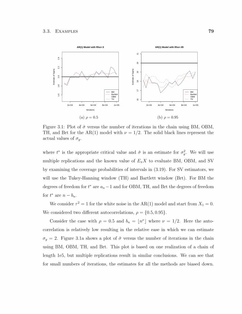
3.3. Examples 79
AR(1) Model with Rho=.5
Iterations
Est
imat
e of
Sig
ma
2e+04 4e+04 6e+04 8e+04 1e+05
1.6
1.8
2.0
2.2
2.4
BMBartlettOBMTH
(a) ρ = 0.5
AR(1) Model with Rho=.95
Iterations
Est
imat
e of
Sig
ma
2e+04 4e+04 6e+04 8e+04 1e+05
1617
1819
2021
BMBartlettOBMTH
(b) ρ = 0.95
Figure 3.1: Plot of σ versus the number of iterations in the chain using BM, OBM,TH, and Brt for the AR(1) model with ν = 1/2. The solid black lines represent theactual values of σg.
where t∗ is the appropriate critical value and σ is an estimate for σ2g . We will use
multiple replications and the known value of EπX to evaluate BM, OBM, and SV
by examining the coverage probabilities of intervals in (3.19). For SV estimators, we
will use the Tukey-Hanning window (TH) and Bartlett window (Brt). For BM the
degrees of freedom for t∗ are an−1 and for OBM, TH, and Brt the degrees of freedom
for t∗ are n− bn.
We consider τ 2 = 1 for the white noise in the AR(1) model and start from X1 = 0.
We considered two different autocorrelations, ρ = 0.5, 0.95.
Consider the case with ρ = 0.5 and bn = bnνc where ν = 1/2. Here the auto-
correlation is relatively low resulting in the relative ease in which we can estimate
σg = 2. Figure 3.1a shows a plot of σ versus the number of iterations in the chain
using BM, OBM, TH, and Brt. This plot is based on one realization of a chain of
length 1e5, but multiple replications result in similar conclusions. We can see that
for small numbers of iterations, the estimates for all the methods are biased down.
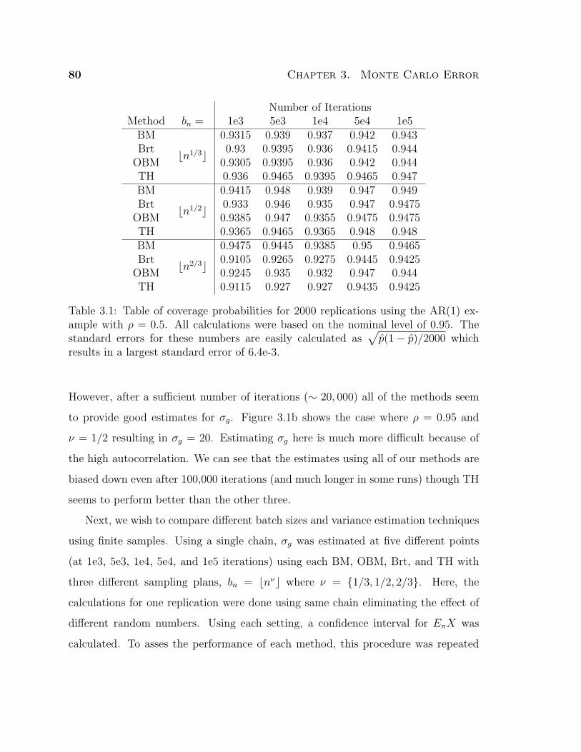
80 Chapter 3. Monte Carlo Error
Number of IterationsMethod bn = 1e3 5e3 1e4 5e4 1e5
BM
bn1/3c
0.9315 0.939 0.937 0.942 0.943Brt 0.93 0.9395 0.936 0.9415 0.944
OBM 0.9305 0.9395 0.936 0.942 0.944TH 0.936 0.9465 0.9395 0.9465 0.947BM
bn1/2c
0.9415 0.948 0.939 0.947 0.949Brt 0.933 0.946 0.935 0.947 0.9475
OBM 0.9385 0.947 0.9355 0.9475 0.9475TH 0.9365 0.9465 0.9365 0.948 0.948BM
bn2/3c
0.9475 0.9445 0.9385 0.95 0.9465Brt 0.9105 0.9265 0.9275 0.9445 0.9425
OBM 0.9245 0.935 0.932 0.947 0.944TH 0.9115 0.927 0.927 0.9435 0.9425
Table 3.1: Table of coverage probabilities for 2000 replications using the AR(1) ex-ample with ρ = 0.5. All calculations were based on the nominal level of 0.95. Thestandard errors for these numbers are easily calculated as
√p(1− p)/2000 which
results in a largest standard error of 6.4e-3.
However, after a sufficient number of iterations (∼ 20, 000) all of the methods seem
to provide good estimates for σg. Figure 3.1b shows the case where ρ = 0.95 and
ν = 1/2 resulting in σg = 20. Estimating σg here is much more difficult because of
the high autocorrelation. We can see that the estimates using all of our methods are
biased down even after 100,000 iterations (and much longer in some runs) though TH
seems to perform better than the other three.
Next, we wish to compare different batch sizes and variance estimation techniques
using finite samples. Using a single chain, σg was estimated at five different points
(at 1e3, 5e3, 1e4, 5e4, and 1e5 iterations) using each BM, OBM, Brt, and TH with
three different sampling plans, bn = bnνc where ν = 1/3, 1/2, 2/3. Here, the
calculations for one replication were done using same chain eliminating the effect of
different random numbers. Using each setting, a confidence interval for EπX was
calculated. To asses the performance of each method, this procedure was repeated
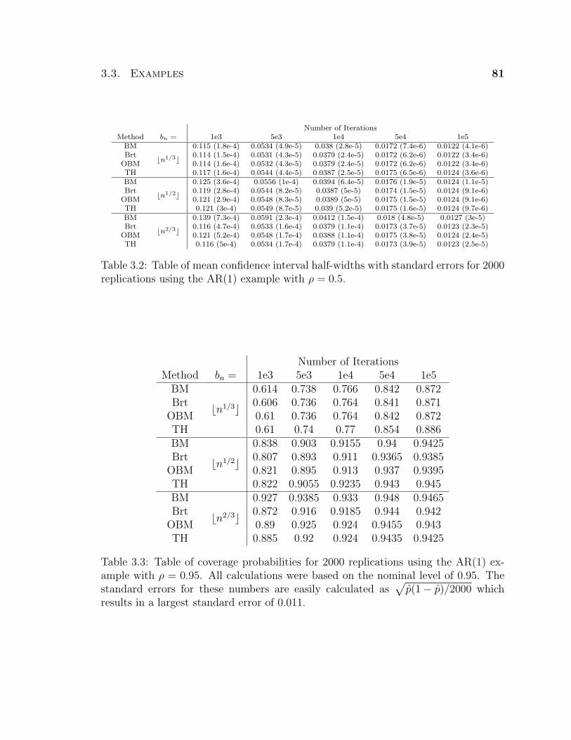
3.3. Examples 81
Number of IterationsMethod bn = 1e3 5e3 1e4 5e4 1e5
BM
bn1/3c
0.115 (1.8e-4) 0.0534 (4.9e-5) 0.038 (2.8e-5) 0.0172 (7.4e-6) 0.0122 (4.1e-6)Brt 0.114 (1.5e-4) 0.0531 (4.3e-5) 0.0379 (2.4e-5) 0.0172 (6.2e-6) 0.0122 (3.4e-6)
OBM 0.114 (1.6e-4) 0.0532 (4.3e-5) 0.0379 (2.4e-5) 0.0172 (6.2e-6) 0.0122 (3.4e-6)TH 0.117 (1.6e-4) 0.0544 (4.4e-5) 0.0387 (2.5e-5) 0.0175 (6.5e-6) 0.0124 (3.6e-6)BM
bn1/2c
0.125 (3.6e-4) 0.0556 (1e-4) 0.0394 (6.4e-5) 0.0176 (1.9e-5) 0.0124 (1.1e-5)Brt 0.119 (2.8e-4) 0.0544 (8.2e-5) 0.0387 (5e-5) 0.0174 (1.5e-5) 0.0124 (9.1e-6)
OBM 0.121 (2.9e-4) 0.0548 (8.3e-5) 0.0389 (5e-5) 0.0175 (1.5e-5) 0.0124 (9.1e-6)TH 0.121 (3e-4) 0.0549 (8.7e-5) 0.039 (5.2e-5) 0.0175 (1.6e-5) 0.0124 (9.7e-6)BM
bn2/3c
0.139 (7.3e-4) 0.0591 (2.3e-4) 0.0412 (1.5e-4) 0.018 (4.8e-5) 0.0127 (3e-5)Brt 0.116 (4.7e-4) 0.0533 (1.6e-4) 0.0379 (1.1e-4) 0.0173 (3.7e-5) 0.0123 (2.3e-5)
OBM 0.121 (5.2e-4) 0.0548 (1.7e-4) 0.0388 (1.1e-4) 0.0175 (3.8e-5) 0.0124 (2.4e-5)TH 0.116 (5e-4) 0.0534 (1.7e-4) 0.0379 (1.1e-4) 0.0173 (3.9e-5) 0.0123 (2.5e-5)
Table 3.2: Table of mean confidence interval half-widths with standard errors for 2000replications using the AR(1) example with ρ = 0.5.
Number of IterationsMethod bn = 1e3 5e3 1e4 5e4 1e5
BM
bn1/3c
0.614 0.738 0.766 0.842 0.872Brt 0.606 0.736 0.764 0.841 0.871
OBM 0.61 0.736 0.764 0.842 0.872TH 0.61 0.74 0.77 0.854 0.886BM
bn1/2c
0.838 0.903 0.9155 0.94 0.9425Brt 0.807 0.893 0.911 0.9365 0.9385
OBM 0.821 0.895 0.913 0.937 0.9395TH 0.822 0.9055 0.9235 0.943 0.945BM
bn2/3c
0.927 0.9385 0.933 0.948 0.9465Brt 0.872 0.916 0.9185 0.944 0.942
OBM 0.89 0.925 0.924 0.9455 0.943TH 0.885 0.92 0.924 0.9435 0.9425
Table 3.3: Table of coverage probabilities for 2000 replications using the AR(1) ex-ample with ρ = 0.95. All calculations were based on the nominal level of 0.95. Thestandard errors for these numbers are easily calculated as
√p(1− p)/2000 which
results in a largest standard error of 0.011.
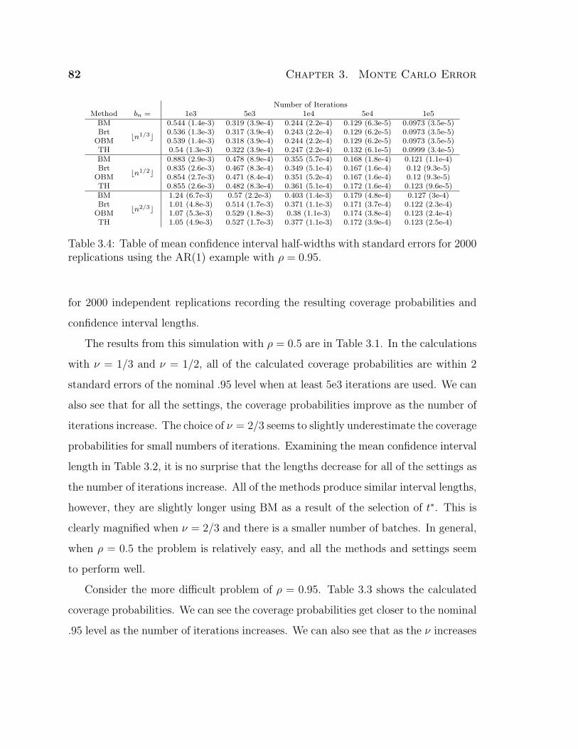
82 Chapter 3. Monte Carlo Error
Number of IterationsMethod bn = 1e3 5e3 1e4 5e4 1e5
BM
bn1/3c
0.544 (1.4e-3) 0.319 (3.9e-4) 0.244 (2.2e-4) 0.129 (6.3e-5) 0.0973 (3.5e-5)Brt 0.536 (1.3e-3) 0.317 (3.9e-4) 0.243 (2.2e-4) 0.129 (6.2e-5) 0.0973 (3.5e-5)
OBM 0.539 (1.4e-3) 0.318 (3.9e-4) 0.244 (2.2e-4) 0.129 (6.2e-5) 0.0973 (3.5e-5)TH 0.54 (1.3e-3) 0.322 (3.9e-4) 0.247 (2.2e-4) 0.132 (6.1e-5) 0.0999 (3.4e-5)BM
bn1/2c
0.883 (2.9e-3) 0.478 (8.9e-4) 0.355 (5.7e-4) 0.168 (1.8e-4) 0.121 (1.1e-4)Brt 0.835 (2.6e-3) 0.467 (8.3e-4) 0.349 (5.1e-4) 0.167 (1.6e-4) 0.12 (9.3e-5)
OBM 0.854 (2.7e-3) 0.471 (8.4e-4) 0.351 (5.2e-4) 0.167 (1.6e-4) 0.12 (9.3e-5)TH 0.855 (2.6e-3) 0.482 (8.3e-4) 0.361 (5.1e-4) 0.172 (1.6e-4) 0.123 (9.6e-5)BM
bn2/3c
1.24 (6.7e-3) 0.57 (2.2e-3) 0.403 (1.4e-3) 0.179 (4.8e-4) 0.127 (3e-4)Brt 1.01 (4.8e-3) 0.514 (1.7e-3) 0.371 (1.1e-3) 0.171 (3.7e-4) 0.122 (2.3e-4)
OBM 1.07 (5.3e-3) 0.529 (1.8e-3) 0.38 (1.1e-3) 0.174 (3.8e-4) 0.123 (2.4e-4)TH 1.05 (4.9e-3) 0.527 (1.7e-3) 0.377 (1.1e-3) 0.172 (3.9e-4) 0.123 (2.5e-4)
Table 3.4: Table of mean confidence interval half-widths with standard errors for 2000replications using the AR(1) example with ρ = 0.95.
for 2000 independent replications recording the resulting coverage probabilities and
confidence interval lengths.
The results from this simulation with ρ = 0.5 are in Table 3.1. In the calculations
with ν = 1/3 and ν = 1/2, all of the calculated coverage probabilities are within 2
standard errors of the nominal .95 level when at least 5e3 iterations are used. We can
also see that for all the settings, the coverage probabilities improve as the number of
iterations increase. The choice of ν = 2/3 seems to slightly underestimate the coverage
probabilities for small numbers of iterations. Examining the mean confidence interval
length in Table 3.2, it is no surprise that the lengths decrease for all of the settings as
the number of iterations increase. All of the methods produce similar interval lengths,
however, they are slightly longer using BM as a result of the selection of t∗. This is
clearly magnified when ν = 2/3 and there is a smaller number of batches. In general,
when ρ = 0.5 the problem is relatively easy, and all the methods and settings seem
to perform well.
Consider the more difficult problem of ρ = 0.95. Table 3.3 shows the calculated
coverage probabilities. We can see the coverage probabilities get closer to the nominal
.95 level as the number of iterations increases. We can also see that as the ν increases
3.3. Examples 83
the confidence intervals become more accurate because the strong correlation in the
model is better captured with larger batch sizes. In this case, the choice of ν = 1/3
performs much worse than the other options analyzed. For ν = 2/3, BM performs
better in terms of coverage probabilities but results in longer confidence intervals (see
Table 3.4). Again, this is a result of the selection of t∗ for BM.
3.3.2 Bayesian Probit Regression
Suppose Y1, . . . , Ym are independent Bernoulli random variables with Pr(Yi = 1) =
Φ(xTi β) where xi is a p × 1 vector of known covariates associated with Yi, β is a
p×1 vector of unknown regression coefficients, and Φ(·) denotes the standard normal
distribution function. Then for yi ∈ 0, 1
Pr(Y1 = y1, . . . , Yn = ym|β) =m∏
i=1
Φ(xTi β)yi
[1− Φ(xT
i β)]1−yi
.
Bayesian inference on β with a flat prior (p-dimensional Lebesgue measure) is common
resulting in
π(β|y) ∝m∏
i=1
Φ(xTi β)yi
[1− Φ(xT
i β)]1−yi
,
which under regularity conditions is proper (Roy and Hobert, 2007).
We will sample from π(β|y) using the PX-DA algorithm of Liu and Wu (1999).
First, let TN(µ, σ2, w) denote a normal distribution with mean µ and variance σ2 that
is truncated to be positive if w = 1 and negative if w = 0. The procedure requires:
1. Draw z1, . . . , zm independently with zi ∼ TN(xTi β, 1, yi).
2. Draw g2 ∼ Γ(
n2, 1
2
∑mi=1
[zi − xT
i (XTX)−1XT z]2)
and set z′ = (gz1, . . . , gzm)T .
3. Draw β′ ∼ N((XTX)−1XT z′, (XTX)−1
).

84 Chapter 3. Monte Carlo Error
βi σβiMCSE
β0 −3.0192 11.830 0.004β1 6.9136 22.654 0.008β2 3.9804 14.765 0.005
Table 3.5: Results from 9e6 iterations for the Bayesian probit regression using theLupus data from van Dyk and Meng (2001). These values were treated as the “truth”for estimating confidence interval coverage probabilities.
We will use the general framework above to analyze the Lupus Data from van Dyk
and Meng (2001). The goal of this example is to predict the occurrence of latent
membranous lupus nephritis using xi1, the difference between IgG3 and IgG4 (im-
munoglobulin G), and xi2, IgA (immunoglobulin A). The response variable is yi, an
indicator of the disease (1 for present). We consider the a Bayesian analysis using a
flat prior of the following model
Pr(Yi = 1) = Φ (β0 + β1xi1 + β2xi2) .
Hence, we are interested in estimating the regression parameters β := (β0, β1, β2).
Chen and Shao (2001) show conditions to ensure the appropriate moment condi-
tions for estimating the posterior expectation of the regression parameters, β. Roy
and Hobert (2007) verify these conditions and show conditions to ensure the chain is
geometrically ergodic.
In the following sections, we will attempt to compare different methods based on
their coverage probabilities. However, this requires the actual value of β which can
never be known in a real example such as this. In an attempt to solve this problem,
we will calculate a very precise estimate of β from one long run, and treat this as the
“truth” when evaluating confidence intervals in future sections. Table 3.5 shows the
calculated values from one long run of 9e6 iterations. MCSEs were calculated using
BM with a batch size of n1/2.
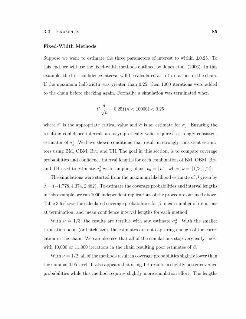
3.3. Examples 85
Fixed-Width Methods
Suppose we want to estimate the three parameters of interest to within ±0.25. To
this end, we will use the fixed-width methods outlined by Jones et al. (2006). In this
example, the first confidence interval will be calculated at 1e4 iterations in the chain.
If the maximum half-width was greater than 0.25, then 1000 iterations were added
to the chain before checking again. Formally, a simulation was terminated when
t∗σ√n
+ 0.25I(n < 10000) < 0.25
where t∗ is the appropriate critical value and σ is an estimate for σg. Ensuring the
resulting confidence intervals are asymptotically valid requires a strongly consistent
estimator of σ2g . We have shown conditions that result in strongly consistent estima-
tors using BM, OBM, Brt, and TH. The goal in this section, is to compare coverage
probabilities and confidence interval lengths for each combination of BM, OBM, Brt,
and TH used to estimate σ2g with sampling plans, bn = bnνc where ν = 1/3, 1/2.
The simulations were started from the maximum likelihood estimate of β given by
β = (−1.778, 4.374, 2.482). To estimate the coverage probabilities and interval lengths
in this example, we ran 1000 independent replications of the procedure outlined above.
Table 3.6 shows the calculated coverage probabilities for β, mean number of iterations
at termination, and mean confidence interval lengths for each method.
With ν = 1/3, the results are terrible with any estimate σ2g . With the smaller
truncation point (or batch size), the estimates are not capturing enough of the corre-
lation in the chain. We can also see that all of the simulations stop very early, most
with 10,000 or 11,000 iterations in the chain resulting poor estimates of β.
With ν = 1/2, all of the methods result in coverage probabilities slightly lower than
the nominal 0.95 level. It also appears that using TH results in slightly better coverage
probabilities while this method requires slightly more simulation effort. The lengths
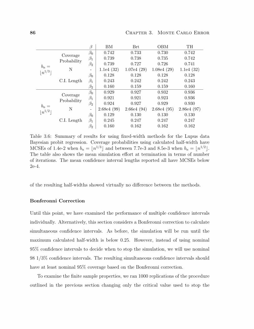
86 Chapter 3. Monte Carlo Error
β BM Brt OBM TH
bn =bn1/3c
CoverageProbability
β0 0.742 0.733 0.730 0.742β1 0.739 0.738 0.735 0.742β2 0.739 0.727 0.726 0.741
N - 1.1e4 (32) 1.07e4 (29) 1.08e4 (29) 1.1e4 (32)
C.I. Lengthβ0 0.128 0.128 0.128 0.128β1 0.243 0.242 0.242 0.243β2 0.160 0.159 0.159 0.160
bn =bn1/2c
CoverageProbability
β0 0.929 0.927 0.932 0.936β1 0.921 0.921 0.923 0.936β2 0.924 0.927 0.929 0.930
N - 2.68e4 (99) 2.66e4 (94) 2.68e4 (95) 2.86e4 (97)
C.I. Lengthβ0 0.129 0.130 0.130 0.130β1 0.245 0.247 0.247 0.247β2 0.160 0.162 0.162 0.162
Table 3.6: Summary of results for using fixed-width methods for the Lupus dataBayesian probit regression. Coverage probabilities using calculated half-width haveMCSEs of 1.4e-2 when bn = bn1/3c and between 7.7e-3 and 8.5e-3 when bn = bn1/2c.The table also shows the mean simulation effort at termination in terms of numberof iterations. The mean confidence interval lengths reported all have MCSEs below2e-4.
of the resulting half-widths showed virtually no difference between the methods.
Bonferonni Correction
Until this point, we have examined the performance of multiple confidence intervals
individually. Alternatively, this section considers a Bonferonni correction to calculate
simultaneous confidence intervals. As before, the simulation will be run until the
maximum calculated half-width is below 0.25. However, instead of using nominal
95% confidence intervals to decide when to stop the simulation, we will use nominal
98 1/3% confidence intervals. The resulting simultaneous confidence intervals should
have at least nominal 95% coverage based on the Bonferonni correction.
To examine the finite sample properties, we ran 1000 replications of the procedure
outlined in the previous section changing only the critical value used to stop the
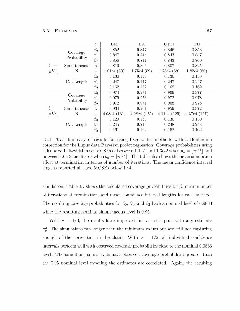
3.3. Examples 87
β BM Brt OBM TH
bn =bn1/3c
CoverageProbability
β0 0.852 0.847 0.846 0.853β1 0.847 0.844 0.843 0.847β2 0.856 0.841 0.843 0.860
Simultaneous β 0.819 0.806 0.807 0.825N - 1.81e4 (59) 1.75e4 (59) 1.75e4 (59) 1.82e4 (60)
C.I. Lengthβ0 0.130 0.130 0.130 0.130β1 0.247 0.247 0.247 0.247β2 0.162 0.162 0.162 0.162
bn =bn1/2c
CoverageProbability
β0 0.974 0.971 0.969 0.977β1 0.975 0.973 0.972 0.978β2 0.972 0.971 0.968 0.978
Simultaneous β 0.964 0.961 0.959 0.972N - 4.08e4 (131) 4.08e4 (125) 4.11e4 (125) 4.37e4 (127)
C.I. Lengthβ0 0.129 0.130 0.130 0.130β1 0.245 0.248 0.248 0.248β2 0.161 0.162 0.162 0.162
Table 3.7: Summary of results for using fixed-width methods with a Bonferonnicorrection for the Lupus data Bayesian probit regression. Coverage probabilities usingcalculated half-width have MCSEs of between 1.1e-2 and 1.3e-2 when bn = bn1/3c andbetween 4.6e-3 and 6.3e-3 when bn = bn1/2c. The table also shows the mean simulationeffort at termination in terms of number of iterations. The mean confidence intervallengths reported all have MCSEs below 1e-4.
simulation. Table 3.7 shows the calculated coverage probabilities for β, mean number
of iterations at termination, and mean confidence interval lengths for each method.
The resulting coverage probabilities for β0, β1, and β2 have a nominal level of 0.9833
while the resulting nominal simultaneous level is 0.95.
With ν = 1/3, the results have improved but are still poor with any estimate
σ2g . The simulations ran longer than the minimum values but are still not capturing
enough of the correlation in the chain. With ν = 1/2, all individual confidence
intervals perform well with observed coverage probabilities close to the nominal 0.9833
level. The simultaneous intervals have observed coverage probabilities greater than
the 0.95 nominal level meaning the estimates are correlated. Again, the resulting
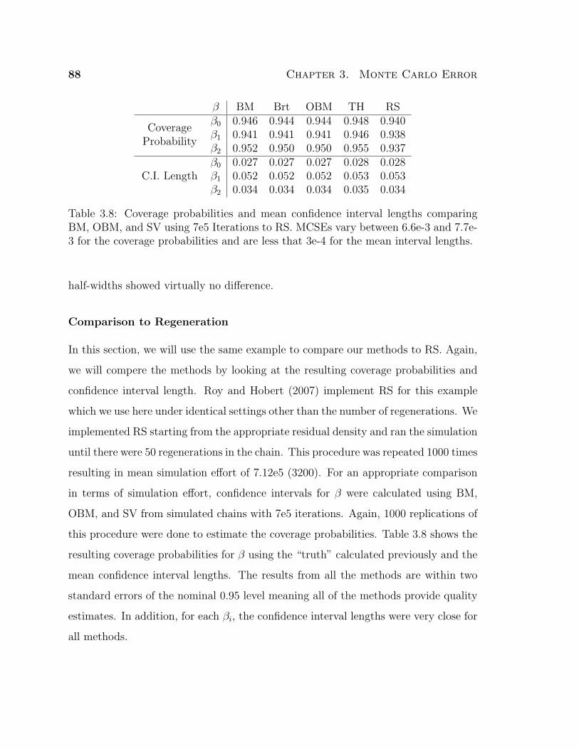
88 Chapter 3. Monte Carlo Error
β BM Brt OBM TH RS
CoverageProbability
β0 0.946 0.944 0.944 0.948 0.940β1 0.941 0.941 0.941 0.946 0.938β2 0.952 0.950 0.950 0.955 0.937
C.I. Lengthβ0 0.027 0.027 0.027 0.028 0.028β1 0.052 0.052 0.052 0.053 0.053β2 0.034 0.034 0.034 0.035 0.034
Table 3.8: Coverage probabilities and mean confidence interval lengths comparingBM, OBM, and SV using 7e5 Iterations to RS. MCSEs vary between 6.6e-3 and 7.7e-3 for the coverage probabilities and are less that 3e-4 for the mean interval lengths.
half-widths showed virtually no difference.
Comparison to Regeneration
In this section, we will use the same example to compare our methods to RS. Again,
we will compere the methods by looking at the resulting coverage probabilities and
confidence interval length. Roy and Hobert (2007) implement RS for this example
which we use here under identical settings other than the number of regenerations. We
implemented RS starting from the appropriate residual density and ran the simulation
until there were 50 regenerations in the chain. This procedure was repeated 1000 times
resulting in mean simulation effort of 7.12e5 (3200). For an appropriate comparison
in terms of simulation effort, confidence intervals for β were calculated using BM,
OBM, and SV from simulated chains with 7e5 iterations. Again, 1000 replications of
this procedure were done to estimate the coverage probabilities. Table 3.8 shows the
resulting coverage probabilities for β using the “truth” calculated previously and the
mean confidence interval lengths. The results from all the methods are within two
standard errors of the nominal 0.95 level meaning all of the methods provide quality
estimates. In addition, for each βi, the confidence interval lengths were very close for
all methods.
3.3. Examples 89
3.3.3 Summary
In our examples, we consider different estimators of σ2g . In general, all of the methods
considered resulted in similar performance for a given simulation setting. Recall,
OBM and Brt are asymptotically equivalent and the simulation results show there is
little difference between the two in finite samples. In our experience, Brt (and SV
methods in general) tended to run slightly faster computationally than OBM. The
TH estimator exhibits very similar behavior to OBM and Brt, though there seems
to be a slight improvement in performance. Confirming the theoretical results from
Section 3.2.3, the estimator from BM was more variable than OBM (Figure 3.1). This
result was consistent in both examples in multiple realizations.
Using the Bayesian probit regression model we compared our methods to RS. The
resulting simulation showed all the methods performed very well. The advantage of
RS is that the actual chain does not need to be stored as the simulation progresses.
However, RS requires a considerable theoretical cost that is likely to dissuade a prac-
titioner. The resulting simulation is also dependent on the length of the regeneration
tours which can become very long as the dimension increases (Johnson and Jones,
2008). In contrast, BM, OBM, and SV are relatively simple to implement though they
can require saving the entire chain. Given the current price of computer memory, this
is clearly not the obstacle it was in the past.
The second simulation goal was to investigate the finite sample behavior of differ-
ent batch size selection. Theoretically, we showed that the batch size should increase
at a rate proportional to n1/3 where the proportionality constant is unknown. In our
examples, using bn = bn1/3c seemed to give very poor results because the batch size
or truncation point was too small. In realistic examples with higher correlations, the
larger batch size bn = bn1/2c worked well agreeing with the previous work of Jones
et al. (2006). Our investigation of bn = bn2/3c worked well in high correlation settings,
though for long chains more computational effort was necessary.
90 Chapter 3. Monte Carlo Error
3.4 Proofs and Calculations
3.4.1 Results for Proof of Lemma 4
This proof is contained in Jones et al. (2006) and extended by Bednorz and La-
tuszynski (2007). The first part of the lemma is an immediate consequence of the
Theorem 4.1 of Philipp and Stout (1975) and the fact that uniformly ergodic Markov
chains enjoy exponentially fast uniform mixing (see Chapter 2). The second part
follows from our Lemma 5 and Theorem 2.1 in Csaki and Csorgo (1995).
Lemma 5. Let X be a Harris ergodic Markov chain on X with invariant distribution
π. Assume that (2.4) holds and that X is geometrically ergodic. If Eπ|g|p+δ <∞ for
some p > 0 and δ > 0, then EQNp1 <∞ and EQS
p1 <∞.
Preliminary Results
In the proof of this Lemma 5, we will require two additional Lemmas.
Lemma 6. (Hobert et al., 2002, Lemma 1) Let X be a Harris ergodic Markov chain
and assume that (2.4) holds. Then for any function h : X∞ 7→ R
Eπ|h(X1, X2, . . . )| ≥ cEQ|h(X1, X2, . . . )|,
where c = Eπs.
Proof. For any measurable set A it follows from (2.4) that
π(A) =
∫X
π(dx)P (x,A) ≥ Q(A)
∫X
π(dx)s(x) (3.20)
and hence π(·) ≥ cQ(·). Next note that
Eπ|h(X1, X2, . . . )| = Eπ [E |h(X1, X2, . . . )| | X1] .
3.4. Proofs and Calculations 91
The inner expectation is a nonnegative function of X1 not depending on the starting
distribution. Thus, we can use (3.20) and the Markov property to obtain
Eπ|h(X1, X2, . . . )| ≥ cEQ [E |h(X1, X2, . . . )| | X1] = cEQ|h(X1, X2, . . . )|.
Lemma 7. (Hobert et al., 2002, Lemma 2) Let X be a Harris ergodic Markov chain
and assume that (2.4) holds. If X is geometrically ergodic, then there exists a β > 1
such that Eπβτ1 <∞.
Proof. First notice that τ1 = mini > 0 : (Xi−1, δi−1) ∈ X× 1; or just the hitting
time on the set X × 1. Also note that X and X ′ converge to stationarity at the
exact same rate, consequently, since X is geometrically ergodic, so is X ′. Now let π′
denote the invariant distribution of X ′ and note that a random vector (X, δ) with
distribution π′ satisfies X ∼ π(·), and, conditional on X, δ|X ∼ Bernoulli(s(X)).
Thus π′(X × 1) = Eπ(s) > 0, and, since X ′ is geometrically ergodic, Theorem 2.5
of Nummelin and Tuominen (1982) then implies that there exists a β > 1 such that
Eπβτ1 <∞.
Corollary 2. Assume the conditions in Lemma 7. For any a > 0
∞∑i=0
[Prπ(τ1 ≥ i+ 1)]a ≤ (Eπβτ1)a
∞∑i=0
β−a(i+1) <∞ .
Proof of Lemma 5
By Lemma 6, it is enough to verify that Eπτp1 <∞ and EπS
p1 <∞. Lemma 7 shows
that Eπτp1 <∞ for any p > 0.

92 Chapter 3. Monte Carlo Error
To show that EπSp1 <∞, we will first note that
C :=((Eπ|g(Xi)|p+δ
) pp+δ
)1/p
<∞ . (3.21)
For p ≥ 1 we use the triangle inequality in Lp, Holder’s inequality, the inequality
in (3.21) and finally Corollary 2.
(EπSp1)
1/p ≤
[Eπ
(τ1−1∑i=0
|g(Xi)|
)p]1/p
=
[Eπ
(∞∑i=0
I(i ≤ τ1 − 1)|g(Xi)|
)p]1/p
≤∞∑i=0
[EπI(i ≤ τ1 − 1)|g(Xi)|p]1/p
≤∞∑i=0
[(EπI(i ≤ τ1 − 1))
δp+δ(Eπ|g(Xi)|p+δ
) pp+δ
]1/p
= C
∞∑i=0
(Pπ(τ1 ≥ i+ 1))δ
p(p+δ) <∞ .
For 0 < p < 1 we can use the fact xp is concave and then proceed similarly as above
to obtain
EπSp1 ≤ Eπ
(∞∑i=0
I(i ≤ τ1 − 1)|g(Xi)|
)p
≤∞∑i=0
EπI(i ≤ τ1 − 1)|g(Xi)|p
= Cp
∞∑i=0
(Pπ(τ1 ≥ i+ 1))δ
p+δ <∞ .
3.4. Proofs and Calculations 93
3.4.2 Results for Proof of Theorem 5
Recall that X = X1, X2, . . . is a Harris ergodic Markov chain. Define the process
Y = Yi = g(Xi) − Eπg for i = 1, 2, 3, . . . with Yj(k) := k−1∑k
i=1 Yj+i for j =
0, . . . , n− bn and k = 1, . . . , bn and Yn := Y1(n) = n−1∑n
i=1 Yi.
Proposition 3. (Damerdji, 1991, Theorem 3.1) Under Assumption 1, there exist
sequences αn(k) and dn such that σ2(n) = 2πfn(0)− dn where
αn(k) = k2∆2wn(k) and
dn = n−1
([bn∑l=1
∆1wn(l)
(l−1∑i=1
Z2i +
n∑i=n−bn+l+1
Z2i
)]
+ 2bn−1∑s=1
[bn−s∑l=1
∆1wn(s+ l)
(l−1∑i=1
ZiZs+i +n−s∑
i=n−bn+l+1
ZiZs+i
)])
where Zi = Yi − Yn for all i = 1, 2, . . . , n and any empty sums are defined to be zero.
Proof. Damerdji (1991) contains a general proof for Proposition 3 that generalizes
this result to all frequencies. This proof contains the specific proof for φ = 0 with
some added details for clarification.
For clarity, we will define wn(k) := wk, ∆1wn(k) := ∆1wk, and ∆2wn(k) := ∆2wk.
Then we can notice that
∆1wl =bn∑k=l
∆2wk , (3.22)
bn∑l=s+1
∆1wl = ws , and (3.23)
bn∑l=1
∆1wl = 1 . (3.24)

94 Chapter 3. Monte Carlo Error
Recall that Zi = Yi − Yn; therefore
(Yj(k)− Yn)2 = k−2((Yj+1 + · · ·+Xj+k)− kYn
)2= k−2
(k∑
l=1
Zj+l
)2
= k−2
(k∑
l=1
Z2j+l + 2
k−1∑s=1
k−s∑l=1
Zj+lZj+l+s
)
and from (3.10) with αn(k) = k2∆2wn(k),
σ2(n) = n−1
n−bn∑j=0
bn∑k=1
k2∆2wk(Yj(k)− Yn)2
= n−1
n−bn∑j=0
bn∑k=1
∆2wk
[k∑
l=1
Z2j+l
]+
[2n−1
n−bn∑j=0
bn∑k=1
∆2wk
k−1∑s=1
k−s∑l=1
Zj+lZj+l+s
].
(3.25)
By permuting sums in (3.25), we will arrive at the characterization. Denote the first
term in (3.25) as A and the second as B. Then we have that
A = n−1
n−bn∑j=0
bn∑k=1
k∑l=1
∆2wkZ2j+l
= n−1
n−bn∑j=0
bn∑l=1
bn∑k=l
∆2wkZ2j+l
= n−1
n−bn∑j=0
bn∑l=1
Z2j+l
bn∑k=l
∆2wk .

3.4. Proofs and Calculations 95
Then at lag s = 0 from (3.8) and (3.22),
A = n−1
n−bn∑j=0
bn∑l=1
∆1wlZ2j+l =
bn∑l=1
∆1wln−1
n−bn∑j=0
Z2j+l
=bn∑l=1
∆1wl
(γn(0)− n−1
(Z2
1 + . . . Z2l−1 + Z2
n−bn+1+l + · · ·+ Z2n
)).
For s ≥ 0, let
an(s) = n−1
bn−s∑l=1
∆1ws+l
(l−1∑i=1
ZiZs+i +n−s∑
i=n−bn+l+1
ZiZs+i
).
Then from (3.24),
A = γn(0)− an(0) .
Now we can turn our attention to B,
B = 2n−1
n−bn∑j=0
bn∑k=1
k−1∑s=1
k−s∑l=1
∆2wkZj+lZj+l+s .
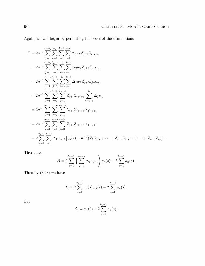
96 Chapter 3. Monte Carlo Error
Again, we will begin by permuting the order of the summations
B = 2n−1
n−bn∑j=0
bn∑k=1
k−1∑s=1
k−s∑l=1
∆2wkZj+lZj+l+s
= 2n−1
n−bn∑j=0
bn−1∑s=1
bn∑k=s
k−s∑l=1
∆2wkZj+lZj+l+s
= 2n−1
bn−1∑s=1
n−bn∑j=0
bn∑k=s
k−s∑l=1
∆2wkZj+lZj+l+s
= 2n−1
bn−1∑s=1
n−bn∑j=0
bn−s∑l=1
Zj+lZj+l+s
bn∑k=l+s
∆2wk
= 2n−1
bn−1∑s=1
n−bn∑j=0
bn−s∑l=1
Zj+lZj+l+s∆1ws+l
= 2n−1
bn−1∑s=1
bn−s∑l=1
n−bn∑j=0
Zj+lZj+l+s∆1ws+l
= 2bn−1∑s=1
bn−s∑l=1
∆1ws+l
[γn(s)− n−1 (ZlZs+l + · · ·+ Zl−1Zs+l−1 + · · ·+ Zn−sZn)
].
Therefore,
B = 2bn−1∑s=1
(bn−s∑l=1
∆1ws+l
)γn(s)− 2
bn−1∑s=1
an(s) .
Then by (3.23) we have
B = 2bn−1∑s=1
γn(s)wn(s)− 2bn−1∑s=1
an(s) .
Let
dn = an(0) + 2bn−1∑s=1
an(s) .
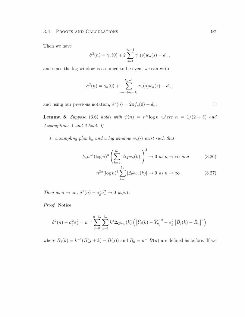
3.4. Proofs and Calculations 97
Then we have
σ2(n) = γn(0) + 2bn−1∑s=1
γn(s)wn(s)− dn ,
and since the lag window is assumed to be even, we can write
σ2(n) = γn(0) +bn−1∑
s=−(bn−1)
γn(s)wn(s)− dn ,
and using our previous notation, σ2(n) = 2πfn(0)− dn.
Lemma 8. Suppose (3.6) holds with ψ(n) = nα log n where α = 1/(2 + δ) and
Assumptions 1 and 2 hold. If
1. a sampling plan bn and a lag window wn(·) exist such that
bnn2α(log n)3
(bn∑
k=1
|∆2wn(k)|
)2
→ 0 as n→∞ and (3.26)
n2α(log n)2
bn∑k=1
|∆2wn(k)| → 0 as n→∞ . (3.27)
Then as n→∞, σ2(n)− σ2g σ
2∗ → 0 w.p.1.
Proof. Notice
σ2(n)− σ2g σ
2∗ = n−1
n−bn∑j=0
bn∑k=1
k2∆2wn(k)([Yj(k)− Yn
]2 − σ2g
[Bj(k)− Bn
]2)
where Bj(k) = k−1(B(j + k)−B(j)) and Bn = n−1B(n) are defined as before. If we

98 Chapter 3. Monte Carlo Error
let
A = k[Yj(k)− σgBj(k)
]=
[(j+k∑i=1
Yi − σgB(j + k)
)−
(j∑
i=1
Yi − σgB(j)
)],
D = B(j + k)−B(j) ,
E = kBn and
F = k[Yn − σgBn
],
then
k(Yj(k)− Yn) = k[Yj(k)− Yn ± σgBj(k)± σgBn
]= k
[Yj(k)− σgBj(k)
]+ σg [B(j + k)−B(j)]
− σgkBn − k[Yn − σgBn
]= A+ σg(D − E)− F .
We can then rewrite
∣∣σ2(n)− σ2g σ
2∗∣∣ ≤ n−1
n−bn∑j=0
bn∑k=1
∣∣∆2wn(k)[(A+ σg(D − E)− F )2 − σ2
g(D − E)2]∣∣
≤ n−1
n−bn∑j=0
bn∑k=1
|∆2wn(k)|[A2 + F 2 + 2σg|AD|+ 2σg|AE|
+2σg|AF |+ 2σg|DF |+ 2σg|EF |] . (3.28)
It suffices to show the 7 terms in (3.28) tend to 0 as n→∞. To this end, we will use
the LIL type results on the increments of Brownian motion from Appendix A.1. Our
assumptions say there exists a strong invariance principle, or there exists a constant

3.4. Proofs and Calculations 99
C such that for all large n∣∣∣∣∣n∑
i=1
g(Xi)− nEπg − σgB(n)
∣∣∣∣∣ ≤ Cnα log n (3.29)
where α = 1/(2 + δ).
1. From (3.29), we can see that
|A| ≤ C(j + k)α log(j + k) + C(j)α log(j) ≤ 2Cnα log n (3.30)
resulting in
n−1
n−bn∑j=0
bn∑k=1
|∆2wn(k)|A2 ≤ 4C2n2α(log n)2
bn∑k=1
|∆2wn(k)| → 0
as n→∞ by (3.27).
2. From (3.29) and the fact that k ≤ bn ≤ n
|F | ≤ Cknα−1 log n , (3.31)
resulting in
n−1
n−bn∑j=0
bn∑k=1
|∆2wn(k)|F 2 ≤ C2n2α−2(log n)2
bn∑k=1
k2 |∆2wn(k)|
≤ C2b2nn2α−2(log n)2
bn∑k=1
|∆2wn(k)| → 0
as n→∞ by (3.27).

100 Chapter 3. Monte Carlo Error
3. From Lemma 16
|D| = |B(j + k)−B(j)|
≤ sup0≤t≤n−bn
sup0≤s≤bn
|B(t+ s)−B(t)|
≤ (1 + ε)
(2bn
(log
n
bn+ log log n
))1/2
≤ 2(1 + ε)b1/2n (log n)1/2 . (3.32)
Combining this with (3.30), we can see
n−1
n−bn∑j=0
bn∑k=1
|∆2wn(k)| 2σg |AD|
≤ 8Cσg(1 + ε)b1/2n nα (log n)3/2
bn∑k=1
|∆2wn(k)| → 0
as n→∞ by (3.26).
4. From Lemma 15
|E| ≤√
2(1 + ε)kn−1/2(log log n)1/2 . (3.33)
Combining this with (3.30), we can see
n−1
n−bn∑j=0
bn∑k=1
|∆2wn(k)| 2σg |AE|
≤ 25/2Cσg(1 + ε)nα−1/2 log n(log log n)1/2
bn∑k=1
k |∆2wn(k)| → 0
as n→∞ by (3.26).

3.4. Proofs and Calculations 101
5. From (3.30) and (3.31) we can write
n−1
n−bn∑j=0
bn∑k=1
|∆2wn(k)| 2 |AF |
≤ 4C2n2α−1(log n)2
bn∑k=1
k |∆2wn(k)| → 0
as n→∞ by (3.27).
6. From (3.32) and (3.31) we can write
n−1
n−bn∑j=0
bn∑k=1
|∆2wn(k)| 2σg |DF |
≤ 4σg(1 + ε)b1/2n nα−1 (log n)3/2
bn∑k=1
k |∆2wn(k)| → 0
as n→∞ by (3.26).
7. From (3.33) and (3.31) we can write
n−1
n−bn∑j=0
bn∑k=1
|∆2wn(k)| 2σg |EF |
≤ 23/2Cσg(1 + ε)nα−3/2 log n(log log n)1/2
bn∑k=1
k2 |∆2wn(k)| → 0
as n→∞ by (3.26).
Hence, all the terms in (3.28) tend to 0 as n→∞ and the lemma is proved.
Lemma 9. Let X be a geometrically ergodic Markov chain with invariant distribution
π and g : X → R be a Borel function with Eπ|g|2+δ+ε <∞ for some δ ≥ 2 and some
ε > 0. If Assumption 2 holds, b−1n log n stays bounded as n→∞, and b−1
n n2α log n→ 0

102 Chapter 3. Monte Carlo Error
as n→∞ where α = 1/(2+δ), then b−1n
∑bn
i=1 Y2i and b−1
n
∑ni=n−bn+1 Y
2i stay bounded
as n→∞ w.p.1.
Proof. First note that if Eπ|g|2 < ∞, then b−1n
∑bn
i=1 Y2i stays bounded as n → ∞
w.p.1 from the Ergodic Theorem.
Consider the sequence Y 2i : i ≥ 1. The stated assumptions imply a Markov chain
CLT holds where σ′g < ∞ is defined as the resulting asymptotic standard deviation.
Lemma 4 implies that∣∣∣∣∣n∑
i=1
Y 2i − nEπY
21 − σ′gB(n)
∣∣∣∣∣ < C ′(ω)n2α log n
for all n > n0.
Then
b−1n
∣∣∣∣∣n∑
i=n−bn+1
Y 2i
∣∣∣∣∣ = b−1n
∣∣∣∣∣n∑
i=1
Y 2i −
n−bn∑i=1
Y 2i
∣∣∣∣∣= b−1
n
∣∣∣∣∣(
n∑i=1
Y 2i − nEπY
21 − σ′gB(n)
)
−
(n−bn∑i=1
Y 2i − (n− bn)EπY
21 − σ′gB(n− bn)
)
+ σ′g (B(n)−B(n− bn)) + bnEπY21
∣∣∣∣∣≤ b−1
n
(2C ′(ω)nα′ log n+ (1 + ε)
(2bn
(log
n
bn+ log log n
))1/2
+ bnEπY21
)= EπY
21 + 2C ′(ω)b−1
n nα′ log n+O((b−1
n log n)1/2)
w.p.1.
Hence, b−1n
∣∣∑ni=n−bn+1 Y
2i
∣∣ stays bounded w.p.1 since b−1n nα′ log n→ 0 as n→∞.
Lemma 10. (Damerdji, 1991, Proposition 4.3) Suppose Assumptions 1 and 2 hold.

3.4. Proofs and Calculations 103
1.
bnn−1
bn∑k=1
k |∆1wn(k)| → 0 as n→∞ ;
2. and b−1n
∑bn
i=1 Y2i and b−1
n
∑ni=n−bn+1 Y
2i stay bounded as n→∞ w.p.1.
Then dn → 0 as n→∞ w.p.1.
Proof. Damerdji (1991) shows a proof for general processes which is expanded here
for clarity. We will show dn → 0 as n→∞ w.p.1 in three steps. Recall
dn = n−1
([bn∑l=1
∆wn(l)
(l−1∑i=1
Z2i +
n∑i=n−bn+l+1
Z2i
)]
+ 2bn−1∑s=1
[bn−s∑l=1
∆wn(s+ l)
(l−1∑i=1
ZiZs+i +n−s∑
i=n−bn+l+1
ZiZs+i
)]), (3.34)
where any empty sums are defined to be zero and Zi = Yi − Yn for all i = 1, 2, . . . , n.
1. Let us put bounds on |dn| such that for l = 1, . . . , bn
l−1∑i=1
Z2i ≤
bn∑i=1
Z2i and
n∑i=n−bn+l+1
Z2i ≤
n∑i=n−bn+1
Z2i .
Then bound the sums in the cross terms using the inequality |ab| ≤ (a2 + b2)/2.
So, for s = 1, . . . , bn and l = 1, . . . , bn − s we have
l−1∑i=1
|ZiZs+i| ≤1
2
l−1∑i=1
(Z2
i + Z2s+i
)≤
bn∑i=1
Z2i
andn−s∑
i=n−bn+l+1
|ZiZs+i| ≤n∑
i=n−bn+1
Z2i .

104 Chapter 3. Monte Carlo Error
Then |dn| can be bounded by
|dn| ≤
(bn∑i=1
Z2i +
n∑i=n−bn+1
Z2i
)n−1
(bn∑l=1
|∆wn(l)|+ 2bn−1∑s=1
bn−s∑l=1
|∆wn(s+ l)|
)
= b−1n
(bn∑i=1
Z2i +
n∑i=n−bn+1
Z2i
)
× n−1bn
(bn∑l=1
|∆wn(l)|+ 2bn−1∑s=1
bn−s∑l=1
|∆wn(s+ l)|
)
= b−1n
(bn∑i=1
Z2i +
n∑i=n−bn+1
Z2i
)(3.35)
× n−1bn
(bn∑l=1
|∆wn(l)|+ 2bn∑
k=1
k |∆wn(k)|
). (3.36)
Then we can see that (3.36) tends to 0 as n→∞ by condition 1. We will show
in the next two steps that (3.35) is bounded implying dn → 0 as n→∞ w.p.1.
2. Here, we will use the fact that b−1n
∑bn
i=1 Y2i and b−1
n
∑ni=n−bn+1 Y
2i stay bounded
as n→∞ w.p.1.
b−1n
bn∑i=1
Z2i = b−1
n
bn∑i=1
Y 2i − 2Ynb
−1n
bn∑i=1
Yi +(Yn
)2.
Then the first term is bounded and by the Cauchy-Schwartz inequality we have
(bn∑i=1
Yi
)2
≤bn∑i=1
Y 2i
which implies∑bn
i=1 Yi is bounded resulting in a bound for the second term.
Finally, the third term is bounded by the assumption of a finite mean through-
out. Therefore, b−1n
∑bn
i=1 Z2i stays bounded for large n w.p.1 and hence the
expression in dn coming from the starting observations goes to 0.

3.4. Proofs and Calculations 105
3. Similarly, we can show b−1n
∑ni=n−bn+1 Z
2i stays bounded for large n w.p.1.
Thus, dn → 0 as n→∞ w.p.1.
3.4.3 Results for Proof of Proposition 2
Lemma 11. (Jones et al., 2006, Lemma 8) Suppose (3.6) holds with ψ(n) = nα log n
where α = 1/(2 + δ) and Assumption 2 holds. If (i) b−1n n2α[log n]3 → 0 as n → ∞
then σ2BM − σ2
g σ2BM → 0 as n→∞ w.p.1.
Proof. Recall that X = X1, X2, . . . is a Harris ergodic Markov chain. Define the
process Y by Yi = g(Xi)− Eπg for i = 1, 2, 3, . . . . Then
σ2BM =
bnan − 1
a−1∑k=0
(Yk − Yn)2
where Yk := 1bn
∑bn
i=1 g(Xkbn+i) for k = 0, . . . , a− 1 and Yn = n−1∑n
i=1 Yi. Since
Yk − Yn = Yk − Yn ± σgBk ± σgBn
we have
∣∣σ2BM− σ2
g σ2BM
∣∣ ≤ bnan − 1
a−1∑k=0
[(Yk − σgBk
)2+(Yn − σgBn
)2+∣∣2 (Yk − σgBk
) (Yn − σgBn
)∣∣+ ∣∣2σg
(Yk − σgBk
)Bk
∣∣+∣∣2σg
(Yk − σgBk
)Bn
∣∣+ ∣∣2σg
(Yn − σgBn
)Bk
∣∣+∣∣2σg
(Yn − σgBn
)Bn
∣∣] .Now we will consider each term in the sum and show that it tends to 0.

106 Chapter 3. Monte Carlo Error
1. Our assumptions say that there exists a constant C such that for all large n∣∣∣∣∣n∑
i=1
g(Xi)− nEπg − σgB(n)
∣∣∣∣∣ < Cnα log n w.p.1. (3.37)
Note that
Yk − σgBk =1
bn
(k+1)bn∑i=1
Yi − σgB((k + 1)bn)
− 1
bn
[kbn∑i=1
Yi − σgB(kbn)
]
and hence by (3.37)
∣∣Yk − σgBk
∣∣ ≤ 1
bn
∣∣∣∣∣∣(k+1)bn∑
i=1
Yi − σgB((k + 1)bn)
∣∣∣∣∣∣+∣∣∣∣∣
kbn∑i=1
Yi − σgB(kbn)
∣∣∣∣∣
<2
bnCnα log n (3.38)
Thenbn
an − 1
a−1∑k=0
(Yk − σgBk
)2< 4C2 an
an − 1b−1n n2α(log n)2 → 0
as n→∞ since Assumption 2 implies an →∞ as n→∞ and (i).
2. Apply (3.37) to obtain
∣∣Yn − σgBn
∣∣ = n−1
∣∣∣∣∣n∑
i=1
Yi − σgB(n)
∣∣∣∣∣ < Cnα−1 log n . (3.39)
Thenbn
an − 1
a−1∑k=0
(Yn − σgBn
)2< C2 an
an − 1
bnn
(log n)2
n1−2α→ 0
as n→∞ by Assumption 2 and since 1− 2α > 0.

3.4. Proofs and Calculations 107
3. By (3.38) and (3.39)
∣∣2 (Yk − σgBk
) (Yn − σgBn
)∣∣ < 4C2b−1n n2α−1(log n)2 .
Thus
bnan − 1
a−1∑k=0
∣∣2 (Yk − σgBk
) (Yn − σgBn
)∣∣ < 4C2 an
an − 1
(log n)2
n1−2α→ 0
as n→∞ by Assumption 2 and since 1− 2α > 0.
4. Since bn ≥ 2, (A.2) and (3.38) together imply
∣∣(Yk − σgBk
)Bk
∣∣ < 23/2C(1 + ε)b−1n
[b−1n n2α(log n)2 log(n/bn)
+b−1n n2α(log n)2 log log n
]1/2.
Hence
bnan − 1
a−1∑k=0
∣∣2σg
(Yk − σgBk
)Bk
∣∣ ≤8σgC(1 + ε)
an
an − 1
[b−1n n2α(log n)2 log(n/bn) + b−1
n n2α(log n)2 log log n]1/2
which tends to 0 as n→∞ by Assumption 2 and (i).
5. By (3.38) and (A.1)
∣∣(Yk − σgBk
)Bn
∣∣ < 4C(1 + ε)b−1n n−1/2+α(log n)(log log n)1/2

108 Chapter 3. Monte Carlo Error
so that
bnan − 1
a−1∑k=0
∣∣2σg
(Yk − σgBk
)Bn
∣∣ <8σgC(1 + ε)
an
an − 1
(log n)(log log n)1/2
n1/2−α→ 0
as n→∞ by Assumption 2 and since 1/2− α > 0.
6. Use (A.2) and (3.39) to get
∣∣(Yn − σgBn
)Bk
∣∣ < √2C(1 + ε)
nα−1 log n
b1/2n
[log(n/bn) + log log n]1/2
and hence using Assumption 2 and (i) shows that as n→∞
bnan − 1
a−1∑k=0
∣∣2σg
(Yn − σgBn
)Bk
∣∣ <4σgC(1 + ε)
an
an − 1
bnn
[b−1n n2α((log n)2 log(n/bn) + (log n)2 log log n)
]1/2 → 0 .
7. Now (A.1) and (3.39) imply
∣∣(Yn − σgBn
)Bn
∣∣ < 2C(1 + ε)n−3/2+α(log n)3/2 .
Hence
bnan − 1
a−1∑k=0
∣∣2σg
(Yn − σgBn
)Bn
∣∣ < 4σgC(1 + ε)an
an − 1
bnn
(log n)3/2
n1/2−α→ 0
as n→∞ by Assumption 2 and since 1/2− α > 0.

3.4. Proofs and Calculations 109
3.4.4 Results for Mean-Square Consistency
Preliminary Results
We require the Generalized Dominated Convergence Theorem.
Lemma 12. (Zeidler, 1990, p. 1015) Suppose
1. ||fn(x)| | ≤ gn(x) for almost all x ∈ M and all n ∈ N where all the functions
gn, g : M → R are integrable and we have the convergence gn → g almost
everywhere on M as n→∞ along with
∫M
gndx→∫
M
gdx as n→∞ ,
2. limn→∞ fn(x) exists for almost all x ∈ M , where fn : M ⊆ RN → Y is mea-
sureable for all n.
Then we have
limn→∞
∫M
fndx =
∫M
limn→∞
fn(x)dx .
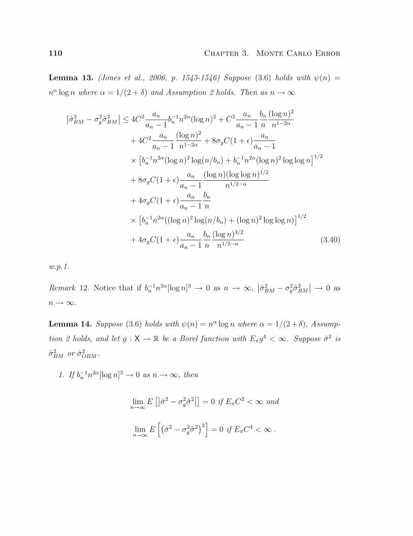
110 Chapter 3. Monte Carlo Error
Lemma 13. (Jones et al., 2006, p. 1545-1546) Suppose (3.6) holds with ψ(n) =
nα log n where α = 1/(2 + δ) and Assumption 2 holds. Then as n→∞
∣∣σ2BM − σ2
g σ2BM
∣∣ ≤ 4C2 an
an − 1b−1n n2α(log n)2 + C2 an
an − 1
bnn
(log n)2
n1−2α
+ 4C2 an
an − 1
(log n)2
n1−2α+ 8σgC(1 + ε)
an
an − 1
×[b−1n n2α(log n)2 log(n/bn) + b−1
n n2α(log n)2 log log n]1/2
+ 8σgC(1 + ε)an
an − 1
(log n)(log log n)1/2
n1/2−α
+ 4σgC(1 + ε)an
an − 1
bnn
×[b−1n n2α((log n)2 log(n/bn) + (log n)2 log log n)
]1/2
+ 4σgC(1 + ε)an
an − 1
bnn
(log n)3/2
n1/2−α(3.40)
w.p.1.
Remark 12. Notice that if b−1n n2α[log n]3 → 0 as n → ∞,
∣∣σ2BM − σ2
g σ2BM
∣∣ → 0 as
n→∞.
Lemma 14. Suppose (3.6) holds with ψ(n) = nα log n where α = 1/(2+ δ), Assump-
tion 2 holds, and let g : X → R be a Borel function with Eπg4 < ∞. Suppose σ2 is
σ2BM or σ2
OBM .
1. If b−1n n2α[log n]3 → 0 as n→∞, then
limn→∞
E[∣∣σ2 − σ2
g σ2∣∣] = 0 if EπC
2 <∞ and
limn→∞
E[(σ2 − σ2
g σ2)2]
= 0 if EπC4 <∞ .

3.4. Proofs and Calculations 111
2. If b−1n n1/2+α[log n]3/2 → 0 as n→∞, then
limn→∞
E
[n
bn
(σ2 − σ2
g σ2)2]
= 0 if EπC4 <∞ .
Proof. We will only prove the first claim for BM as the proof of the others are similar.
From Lemma 13 there exists an integer N0 and functions g1 and g2 such that
|σ2BM − σ2
g σ2BM | = |σ2
BM − σ2g σ
2BM |I(0 ≤ n ≤ N0) + |σ2
BM − σ2g σ
2BM |I(N0 < n)
≤ |σ2BM − σ2
g σ2BM |I(0 ≤ n ≤ N0) + [C2g1(n) + Cg2(n)]I(N0 < n)
:= gn(X1, . . . Xn, B(0), . . . , B(n)) .
Now
Egn(X1, . . . Xn, B(0), . . . , B(n)) = I(0 ≤ n ≤ N0)E|σ2BM − σ2
g σ2BM |
+ [g1(n)E(C2) + g2(n)E(C)]I(N0 < n)
and since Lemma 23 and our assumptions on the moments of g imply
E|σ2BM − σ2
g σ2BM | ≤ Eσ2
BM + σ2gEσ
2BM = Eσ2
BM + σ2g <∞
it follows from our assumptions on the moments of C that E|gn| <∞. Next observe
that as n→∞, we have gn → 0 w.p.1 and Egn → 0 by Lemma 13. From Lemma 11
we have that |σ2BM−σ2
g σ2BM | → 0 w.p.1 as n→∞. An application of the Generalized
Dominated Convergence Theorem implies, as n→∞,
E[∣∣σ2
BM − σ2g σ
2BM
∣∣]→ 0 .
The second result for BM is similar if (3.40) is multiplied through by (n/bn)1/2.
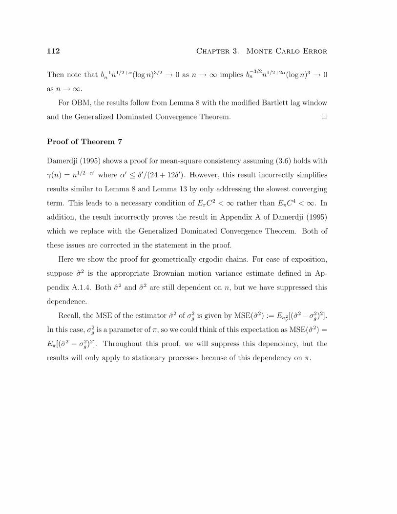
112 Chapter 3. Monte Carlo Error
Then note that b−1n n1/2+α(log n)3/2 → 0 as n → ∞ implies b
−3/2n n1/2+2α(log n)3 → 0
as n→∞.
For OBM, the results follow from Lemma 8 with the modified Bartlett lag window
and the Generalized Dominated Convergence Theorem.
Proof of Theorem 7
Damerdji (1995) shows a proof for mean-square consistency assuming (3.6) holds with
γ(n) = n1/2−α′ where α′ ≤ δ′/(24 + 12δ′). However, this result incorrectly simplifies
results similar to Lemma 8 and Lemma 13 by only addressing the slowest converging
term. This leads to a necessary condition of EπC2 < ∞ rather than EπC
4 < ∞. In
addition, the result incorrectly proves the result in Appendix A of Damerdji (1995)
which we replace with the Generalized Dominated Convergence Theorem. Both of
these issues are corrected in the statement in the proof.
Here we show the proof for geometrically ergodic chains. For ease of exposition,
suppose σ2 is the appropriate Brownian motion variance estimate defined in Ap-
pendix A.1.4. Both σ2 and σ2 are still dependent on n, but we have suppressed this
dependence.
Recall, the MSE of the estimator σ2 of σ2g is given by MSE(σ2) := Eσ2
g[(σ2−σ2
g)2].
In this case, σ2g is a parameter of π, so we could think of this expectation as MSE(σ2) =
Eπ[(σ2 − σ2g)
2]. Throughout this proof, we will suppress this dependency, but the
results will only apply to stationary processes because of this dependency on π.

3.4. Proofs and Calculations 113
1. First, we will show limn→∞nbn
Var(σ2) = 43σ4
g as n→∞. First, one can write
Var(σ2) = E[(
(σ2 − σ2g σ
2) + σ2g(σ
2 − Eσ2)− (Eσ2 − σ2gEσ
2))2]
= σ4gE[(σ2 − Eσ2)2
]+ E
[((σ2 − σ2
g σ2)− E(σ2 − σ2
g σ2))2]
+ 2σ2gE[(σ2 − Eσ2)
((σ2 − σ2
g σ2)− E(σ2 − σ2
g σ2)]
= σ4gVar(σ2) + η , (3.41)
where
η = Var(σ2 − σ2
g σ2)
+ 2σ2gE[(σ2 − Eσ2)(σ2 − σ2
g σ2)].
Using Lemma 23, (3.41) reduces to
Var(σ2) = cσ4g
bnn
+ o
(bnn
)+ η ,
where c = 2 for BM and c = 4/3 for OBM.
To finish the proof of this part of the theorem, we will show that η → 0 as n→
∞. We can simplify the expression of η using the Cauchy-Schwarz inequality
and the fact that Var(X) ≤ EX2,
|η| =∣∣Var
(σ2 − σ2
g σ2)
+ 2σ2gE[(σ2 − Eσ2)(σ2 − σ2
g σ2)]∣∣
≤ E[(σ2 − σ2
g σ2)2]
+ 2σ2g
(E[(σ2 − σ2
g σ2)2]
Var(σ2))1/2
,
which tends to zero as a result of Proposition 14 and (A.12).
2. Next, we will show Bias(σ2) → 0 as n→∞.

114 Chapter 3. Monte Carlo Error
Lemma 23 shows that E [σ2] = 1. We can use this fact with Lemma 14 to get
Bias(σ2) = E(σ2)− σ2g
≤ E[∣∣σ2 − σ2
g σ2∣∣] ,
which tends to zero as n→∞.
3. Clearly, MSE(σ2) → 0 as n→∞ from the first two parts of the theorem.
Proof of Theorem 8
Recall σ2 is defined in Appendix A.1.4. Using (A.12) from Lemma 23, (3.41) reduces
ton
bnVar(σ2) = cσ4
g + o (1) +n
bnη ,
where c = 2 for BM and c = 4/3 for OBM.
To finish the proof, we will show that nbnη → 0 as n→∞. Again, we can simplify
the expression using the Cauchy-Schwarz inequality and the fact that Var(X) ≤ EX2,
n
bn|η| = n
bn
∣∣Var(σ2 − σ2
g σ2)
+ 2σ2gE[(σ2 − Eσ2)(σ2 − σ2
g σ2)]∣∣
≤ E
[n
bn
(σ2 − σ2
g σ2)2]
+ 2σ2g
(E
[n
bn
(σ2 − σ2
g σ2)2] n
bnVar
(σ2))1/2
,
which tends to zero as a result of Lemma 14 and (A.12).
Chapter 4
Subsampling
We have seen several approaches for dealing with ergodic averages and their corre-
sponding standard errors. Very little formal attention has been given to quantities
that cannot be expressed as an ergodic average. This is somewhat surprising con-
sidering empirical quantiles of the posterior distribution are commonly reported in
MCMC literature. For this reason, we introduce subsampling (Politis et al., 1999) for
time–series data and illustrate its use in two examples.
4.1 Introduction
Suppose we want to find the value of some functional θ := θπ where π is a probability
distribution with support X. Our discussion to this point only applies when θ = Eπg.
How can we extend these ideas to characteristics of the target distribution that cannot
be represented as ergodic averages? For example, θ might be the qth quantile of π.
Usually in the MCMC literature, when θ is a quantile what is nearly always meant
is that it is a quantile of one of the univariate marginal distributions associated with
π. The natural estimate of θ is simply the sample quantile from the observed Markov
chain. For a general quantity, consider
θn = θ (X1, . . . , Xn) (4.1)
115
116 Chapter 4. Subsampling
as the appropriate estimate of θ. As before, θn is only a point estimate for the quantity
of interest and we would like to assess the MCSE of θn.
First, consider the sampling distribution of θn, Carlstein (1986) provides one set
of conditions for asymptotic normality for a general statistic under non-trivial depen-
dence. Here, we will present one corollary of his results for quantiles in the context
of a stationary Markov chain. The relationship between the required mixing con-
ditions from Carlstein (1986) and those stated here can be found in Section 2.4.2.
Let us define for κ ∈ [1/n, 1] the statistic Zib(κ) to be the [κn]th ordered element of
Xi+1, Xi+2, . . . , Xi+b. If we consider a subsample from X of length bn = b where we
are suppressing the dependency on n (though this is not necessary in general), then
Proposition 4 gives us joint asymptotic normality between the same quantile from
the sample and the subsample, Z0n(κ) and Zi
b(κ) respectively.
Proposition 4. (Carlstein, 1986, Corollary 10) Let X1 have an absolutely continuous
strictly increasing cdf F , with derivative f . Let Fi(X1, Xi) be the joint cdf of (X1, Xi).
Define k := F−1(κ). If f(k) > 0 and X is geometrically ergodic, then
ν :=∞∑
i=−∞
[Fi(k, k)− κ2
]<∞ .
If ν > 0 and tib :=√b(Zi
b(κ) − k) then for any sequence n satisfying b/n → ρ2 and
n ≥ i+ b ≥ b→∞ t0n
tib
d→ N
0
0
,
σ2 ρσ2
ρσ2 σ2
, for all ρ2 ∈ (0, 1) ,
where σ2 = ν/f 2(k).
Carlstein (1986) gives a more general result that is used by Politis et al. (1999) to
address these questions for a general statistic. Applying this theorem requires further
4.1. Introduction 117
work to estimate σ2. To this end, we will focus our attention on the block bootstrap
and subsampling methods.
4.1.1 Non-overlapping Block Bootstrap
While there has been little investigation of the utility of bootstrap methods in the con-
text of MCMC there has been a substantial amount of work on using bootstrap meth-
ods for stationary time–series. Some of this work is appropriate for use in MCMC; see
e.g., Bertail and Clemencon (2006), Buhlmann (2002), Datta and McCormick (1993),
Politis (2003). Efron and Tibshirani (1993) provide a thorough introduction to the
bootstrap.
One of the simplest approaches is to use a non-overlapping block resampling
scheme to estimate the Monte Carlo standard error of θn. Davison and Hinkley
(1997) provide an overview of this technique. The basic idea is to split the Markov
chain, X, into a non-overlapping blocks of length b, where we suppose the algorithm
is run for a total of n = ab iterations where a = an and b = bn are functions of
n. We will then sample the blocks independently with replacement and with equal
probability and put these blocks together (end to end) to form a new series. We will
use this new series to estimate θ yielding a single bootstrap replicate θ∗n. Repeating
this procedure p times results in p independent and identically distributed estimates;
or θ∗n,1, θ
∗n,2, . . . , θ
∗n,p
.
Using the p replicates, we can appeal to classical bootstrap results to estimate the
standard error of θn by defining
σ2B =
1
p− 1
p∑j=1
(θ∗n,j − θ∗n)2 where θ∗n =1
p
p∑j=1
θ∗n,j .
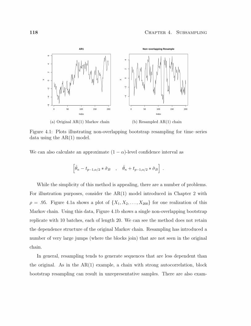
118 Chapter 4. Subsampling
AR1
Index
X
0 50 100 150 200
−6
−4
−2
02
46
(a) Original AR(1) Markov chain
Non−overlapping Resample
Index
X
0 50 100 150 200
−4
−2
02
4
(b) Resampled AR(1) chain
Figure 4.1: Plots illustrating non-overlapping bootstrap resampling for time–seriesdata using the AR(1) model.
We can also calculate an approximate (1− α)-level confidence interval as
[θn − tp−1,α/2 ∗ σB , θn + tp−1,α/2 ∗ σB
].
While the simplicity of this method is appealing, there are a number of problems.
For illustration purposes, consider the AR(1) model introduced in Chapter 2 with
ρ = .95. Figure 4.1a shows a plot of X1, X2, . . . , X200 for one realization of this
Markov chain. Using this data, Figure 4.1b shows a single non-overlapping bootstrap
replicate with 10 batches, each of length 20. We can see the method does not retain
the dependence structure of the original Markov chain. Resampling has introduced a
number of very large jumps (where the blocks join) that are not seen in the original
chain.
In general, resampling tends to generate sequences that are less dependent than
the original. As in the AR(1) example, a chain with strong autocorrelation, block
bootstrap resampling can result in unrepresentative samples. There are also exam-
4.1. Introduction 119
ples (in time–series applications) that “can lead to catastrophically bad resampling
approximations” (Davison and Hinkley, 1997, p. 397). Additionally, we found block
resampling to be extremely computationally intensive even in relatively easy MCMC
problems. With these problems in mind, the non-overlapping block bootstrap was
not pursued.
4.1.2 Subsampling
This section will provide a brief overview of subsampling methods for dependent
data taken from Politis et al. (1999). We will use this framework to estimate the
Monte Carlo standard error of θn and calculate an appropriate confidence interval.
The benefit of subsampling (SUB) methods presented by Politis et al. (1999) are
their generality. Here we will focus on SUB for MCMC. Section 2.4.2 outlines the
connections between the mixing conditions as stated by Politis et al. (1999) and the
presentation here in an MCMC context.
Subsampling differs from the traditional bootstrap in that we are taking samples
(or blocks) of size b without replacement from the initial sample of size n. Typically,
b << n, and in the case of time–series data, there are n − b + 1 such subsamples.
Notice, if we assume X1 is a draw from π, then the different blocks are identically
distributed, though they are clearly still dependent. If we are interested in estimating
θ, we can define the estimator based on the subsample Xi, . . . , Xi+b−1 as
θ∗n,b,i = θ(Xi, . . . , Xi+b−1) for i = 1, . . . , n− b+ 1 .
Then define Jb,i to be the sampling distribution of τb(θ∗n,b,i− θ) where τb is the appro-
priate normalizing constant (which may be unknown). Simplifying notation slightly,
define θn := θ∗n,n,1, the estimator from the whole sample as in (4.1). Then define
Jn := Jn,1 to be sampling distribution of τn(θn − θ) with τn equal to the appropriate

120 Chapter 4. Subsampling
normalizing constant. The corresponding cumulative distribution function is
Jb,i(x) = Prτb(θ∗n,b,i − θ) ≤ x .
We will approximate Jn(x) := Jn,1(x) with the empirical distribution, namely
Ln,b(x) =1
n− b+ 1
n−b+1∑i=1
Iτb(θ∗n,b,i − θ) ≤ x ,
where I is the usual indicator function on Z+. Then, the main assumption needed to
consistently estimate Jn is as follows.
Assumption 3. (Politis et al., 1999, Assumption 4.2.1) There exists a limiting law J
such that
1. Jn converges weakly to J as n→∞, and
2. for every continuity point x of J and for any sequences n, b with n, b→∞ and
b/n→ 0, we have 1n−b+1
∑n−b+1i=1 Jb,i(x) → J(x).
The first condition states that our estimator, properly normalized, has a limiting
distribution. Politis et al. (1999) state “it is hard to conceive of any asymptotic
theory free of such a requirement.” While this may be the case, this is not always a
trivial assumption to verify. If θ = Eπg, then we can appeal to a CLT, but if we are
interested in the case where θ is a quantile (or some other function), it is not entirely
clear how to verify this. Currently, this is an open question, though Proposition 4
from Carlstein (1986) may provide an initial direction.
The second condition states that, for large n, the distribution functions for the
subsamples will on average be close to the distribution function for the entire sam-
ple. Notice that if we assume stationarity, the second part of the assumption is not
necessary.
4.1. Introduction 121
Proposition 5 is stated without proof and follows directly from Theorem 4.2.1 of
Politis et al. (1999). This result allows us to construct a theoretically valid general
confidence interval.
Proposition 5. Suppose Assumption 3 holds and that τb/τn → 0, b/n → 0, and
b→∞ as n→∞. Also assume that X is geometrically ergodic.
1. If x is a continuity point of J(·), then Ln,b(x) → J(x) in probability.
2. If J(·) is continuous, then supx |Ln,b(x)− J(x)| → 0 in probability.
3. For α ∈ (0, 1), let
cn,b(1− α) = infx : Ln,b(x) ≥ 1− α .
Correspondingly, define
cπ(1− α) = infx : J(x) ≥ 1− α .
If J(·) is continuous at cπ(1− α), then
Prτn(θn − θ) ≤ cn,b(1− α) → 1− α as n→∞ .
Thus, the asymptotic coverage probability of the interval [θn− τ−1n cn,b(1−α),∞)
is the nominal level 1−α. Politis et al. (1999) further extend this result for two-sided
symmetric and equal-tailed intervals, where
[θn − τ−1n cn,b(1− α/2) , θn + τ−1
n cn,b(α/2)] , (4.2)
is a level 1− α two-sided equal-tailed interval.
122 Chapter 4. Subsampling
Next, we will consider estimating the variance of θn. First, we will define the
estimator
σ2SUB =
τ 2b
τ 2n
n
n− b+ 1
n−b+1∑i=1
(θ∗n,b,i − θ∗n,b,·)2 , (4.3)
where
θ∗n,b,· =1
n− b+ 1
n−b+1∑i=1
θ∗n,b,i .
Remark 13. If θ = Eπg, then the estimator from SUB in (4.3) is asymptotically
equivalent to the estimator from OBM in (3.12).
Remark 14. Estimating τn when the limiting distribution converges slower than a√n-rate is an open question. Politis et al. (1999) give a method to estimate τn but
there has been no investigation of this in the context of MCMC.
The following theorem gives conditions for the consistency of σ2SUB. Define the
normalized estimator as Tn := τn(θn − E(θn)).
Proposition 6. Let X be a Harris ergodic Markov chain with invariant distribution
π. Further suppose X is geometrically ergodic. Assume that τb/τn → 0, b/n → 0,
and b→∞ as n→∞. Also assume that
1. (Tn)4 are uniformly integrable,
2. nn−b+1
∑n−b+1i=1 Var(τbθ
∗n,b,i) → σ2,
Then σ2SUB is a consistent estimator of σ2.
The proof follows directly from Lemma 4.6.1 of Politis et al. (1999). Again, the
obvious question is how to verify the necessary assumptions? This again is an open
research question, and a clear direction for future work.
In our examples we take bn = bn1/2c as in our analysis using BM. We note that
in our experience subsampling requires approximately the same computational effort
4.2. Stopping the Simulation 123
as BM (when programmed efficiently). Both of these methods are much less compu-
tationally intensive than the traditional bootstrap. For now, we will restrict our use
of subsampling to when θ is a quantile.
4.2 Stopping the Simulation
In this section we consider two formal approaches to terminating the simulation when
estimating general quantities. The first is based on calculating MCSEs and is a
generalization of the approach used previously. The second is based on the Gelman-
Rubin diagnostic (GRD) introduced in Chapter 1. As we have previously seen, GRD
and MCSEs are used to stop the simulation in a similar manner. After n iterations
either the value of the GRD or MCSE is calculated and if it isn’t sufficiently small
then we continue to run the chain until either value has met a user-specified criterion.
4.2.1 Fixed-Width Methods
In the previous chapters we suggested stopping the simulation when the MCSE of
gn is sufficiently small. In this section, we simply generalize this approach to θn. Of
course, we may have to check whether this criterion is met many times, hence the
procedure remains sequential.
Given an estimate of the Monte Carlo standard error of θn, say σ2/√n, we can
form a confidence interval for θ. If this interval is too large then the value of n
is increased and simulation continues until the interval is sufficiently small. The
procedure is terminated when
t∗σ2
SUB√n
+ p(n) ≤ ε (4.4)
where t∗ is an appropriate quantile, p(n) = εI(n ≤ n∗) where, n∗ > 0 is fixed, I is
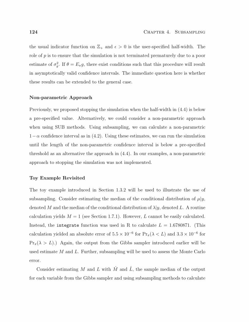
124 Chapter 4. Subsampling
the usual indicator function on Z+ and ε > 0 is the user-specified half-width. The
role of p is to ensure that the simulation is not terminated prematurely due to a poor
estimate of σ2g . If θ = Eπg, there exist conditions such that this procedure will result
in asymptotically valid confidence intervals. The immediate question here is whether
these results can be extended to the general case.
Non-parametric Approach
Previously, we proposed stopping the simulation when the half-width in (4.4) is below
a pre-specified value. Alternatively, we could consider a non-parametric approach
when using SUB methods. Using subsampling, we can calculate a non-parametric
1−α confidence interval as in (4.2). Using these estimates, we can run the simulation
until the length of the non-parametric confidence interval is below a pre-specified
threshold as an alternative the approach in (4.4). In our examples, a non-parametric
approach to stopping the simulation was not implemented.
Toy Example Revisited
The toy example introduced in Section 1.3.2 will be used to illustrate the use of
subsampling. Consider estimating the median of the conditional distribution of µ|y,
denotedM and the median of the conditional distribution of λ|y, denoted L. A routine
calculation yields M = 1 (see Section 1.7.1). However, L cannot be easily calculated.
Instead, the integrate function was used in R to calculate L = 1.6780871. (This
calculation yielded an absolute error of 5.5× 10⁻⁶ for Prπ(λ < L) and 3.3× 10⁻⁶ for
Prπ(λ > L).) Again, the output from the Gibbs sampler introduced earlier will be
used estimate M and L. Further, subsampling will be used to assess the Monte Carlo
error.
Consider estimating M and L with M and L, the sample median of the output
for each variable from the Gibbs sampler and using subsampling methods to calculate
4.2. Stopping the Simulation 125
SUB1
Estimate of M
Freq
uenc
y
0.90 0.95 1.00 1.05 1.10
050
100
150
(a) SUB1, with a cutoff of ε = 0.06.
SUB2
Estimate of M
Freq
uenc
y
0.90 0.95 1.00 1.05 1.10
020
4060
8010
0
(b) SUB2, with a cutoff of ε = 0.04.
GRD1
Estimate of M
Freq
uenc
y
0.90 0.95 1.00 1.05 1.10
020
4060
80
(c) GRD1, 2 chains and δ = 1.1.
GRD3
Estimate of M
Freq
uenc
y
0.90 0.95 1.00 1.05 1.10
050
100
150
200
(d) GRD3, 2 chains and δ = 1.005.
GRD2
Estimate of M
Freq
uenc
y
0.90 0.95 1.00 1.05 1.10
020
4060
8010
012
014
0
(e) GRD2, 4 chains and δ = 1.1.
GRD4
Estimate of M
Freq
uenc
y
0.90 0.95 1.00 1.05 1.10
050
100
150
(f) GRD4, 4 chains and δ = 1.005.
Figure 4.2: Histograms from 1000 replications estimating M for the toy example ofSection 1.3.2 with SUB and GRD. Simulation sample sizes are given in Table 4.3.
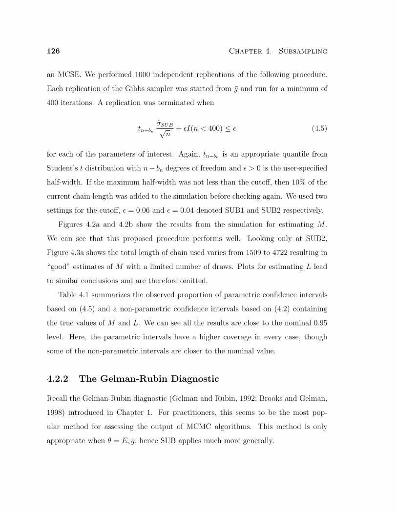
126 Chapter 4. Subsampling
an MCSE. We performed 1000 independent replications of the following procedure.
Each replication of the Gibbs sampler was started from y and run for a minimum of
400 iterations. A replication was terminated when
tn−bn
σSUB√n
+ εI(n < 400) ≤ ε (4.5)
for each of the parameters of interest. Again, tn−bn is an appropriate quantile from
Student’s t distribution with n− bn degrees of freedom and ε > 0 is the user-specified
half-width. If the maximum half-width was not less than the cutoff, then 10% of the
current chain length was added to the simulation before checking again. We used two
settings for the cutoff, ε = 0.06 and ε = 0.04 denoted SUB1 and SUB2 respectively.
Figures 4.2a and 4.2b show the results from the simulation for estimating M .
We can see that this proposed procedure performs well. Looking only at SUB2,
Figure 4.3a shows the total length of chain used varies from 1509 to 4722 resulting in
“good” estimates of M with a limited number of draws. Plots for estimating L lead
to similar conclusions and are therefore omitted.
Table 4.1 summarizes the observed proportion of parametric confidence intervals
based on (4.5) and a non-parametric confidence intervals based on (4.2) containing
the true values of M and L. We can see all the results are close to the nominal 0.95
level. Here, the parametric intervals have a higher coverage in every case, though
some of the non-parametric intervals are closer to the nominal value.
4.2.2 The Gelman-Rubin Diagnostic
Recall the Gelman-Rubin diagnostic (Gelman and Rubin, 1992; Brooks and Gelman,
1998) introduced in Chapter 1. For practitioners, this seems to be the most pop-
ular method for assessing the output of MCMC algorithms. This method is only
appropriate when θ = Eπg, hence SUB applies much more generally.
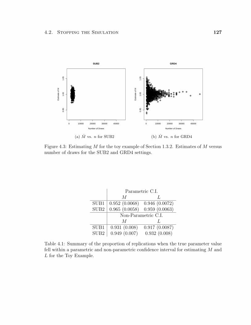
4.2. Stopping the Simulation 127
0 10000 20000 30000 40000
0.95
1.00
1.05
SUB2
Number of Draws
Est
imat
e of
M
(a) M vs. n for SUB2
0 10000 20000 30000 40000
0.95
1.00
1.05
GRD4
Number of Draws
Est
imat
e of
M(b) M vs. n for GRD4
Figure 4.3: Estimating M for the toy example of Section 1.3.2. Estimates of M versusnumber of draws for the SUB2 and GRD4 settings.
Parametric C.I.M L
SUB1 0.952 (0.0068) 0.946 (0.0072)SUB2 0.965 (0.0058) 0.959 (0.0063)
Non-Parametric C.I.M L
SUB1 0.931 (0.008) 0.917 (0.0087)SUB2 0.949 (0.007) 0.932 (0.008)
Table 4.1: Summary of the proportion of replications when the true parameter valuefell within a parametric and non-parametric confidence interval for estimating M andL for the Toy Example.
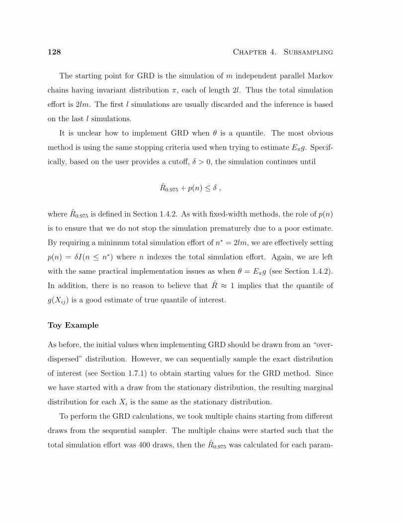
128 Chapter 4. Subsampling
The starting point for GRD is the simulation of m independent parallel Markov
chains having invariant distribution π, each of length 2l. Thus the total simulation
effort is 2lm. The first l simulations are usually discarded and the inference is based
on the last l simulations.
It is unclear how to implement GRD when θ is a quantile. The most obvious
method is using the same stopping criteria used when trying to estimate Eπg. Specif-
ically, based on the user provides a cutoff, δ > 0, the simulation continues until
R0.975 + p(n) ≤ δ ,
where R0.975 is defined in Section 1.4.2. As with fixed-width methods, the role of p(n)
is to ensure that we do not stop the simulation prematurely due to a poor estimate.
By requiring a minimum total simulation effort of n∗ = 2lm, we are effectively setting
p(n) = δI(n ≤ n∗) where n indexes the total simulation effort. Again, we are left
with the same practical implementation issues as when θ = Eπg (see Section 1.4.2).
In addition, there is no reason to believe that R ≈ 1 implies that the quantile of
g(Xij) is a good estimate of true quantile of interest.
Toy Example
As before, the initial values when implementing GRD should be drawn from an “over-
dispersed” distribution. However, we can sequentially sample the exact distribution
of interest (see Section 1.7.1) to obtain starting values for the GRD method. Since
we have started with a draw from the stationary distribution, the resulting marginal
distribution for each Xi is the same as the stationary distribution.
To perform the GRD calculations, we took multiple chains starting from different
draws from the sequential sampler. The multiple chains were started such that the
total simulation effort was 400 draws, then the R0.975 was calculated for each param-
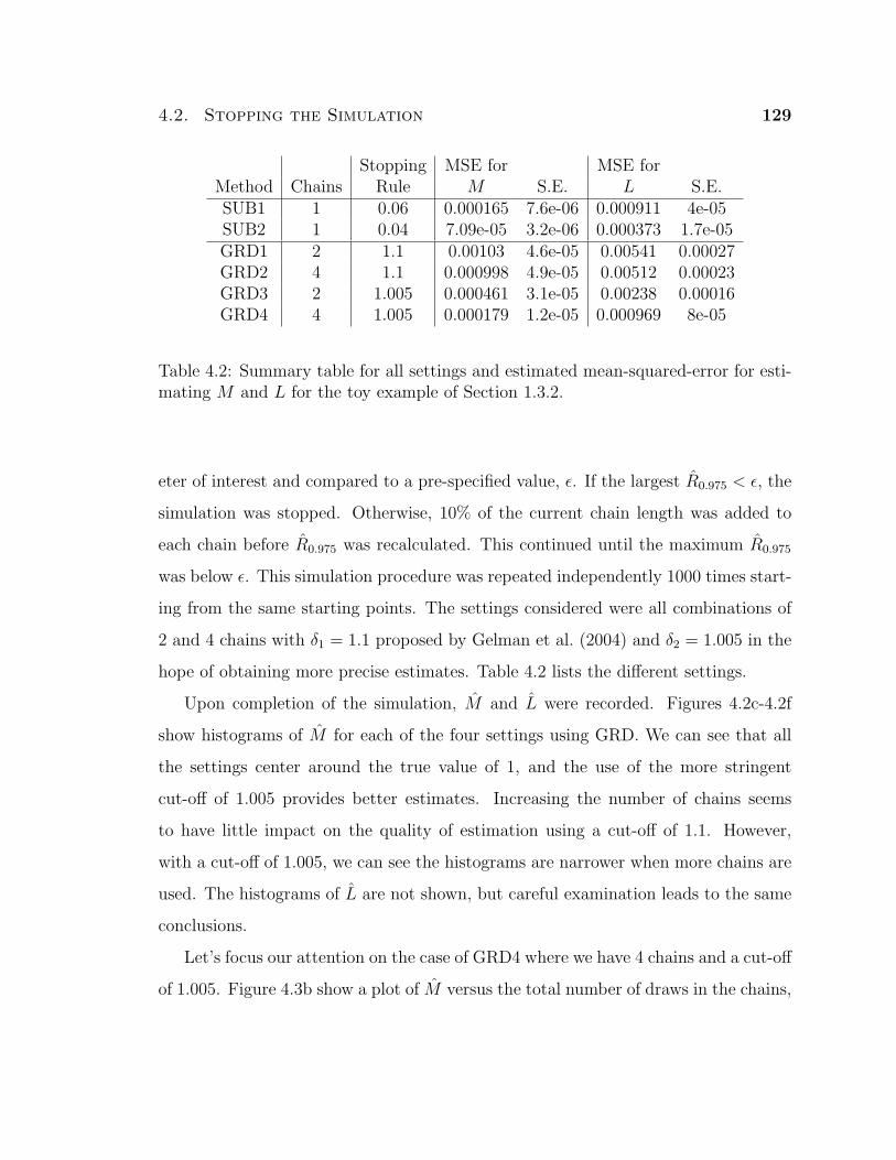
4.2. Stopping the Simulation 129
Stopping MSE for MSE forMethod Chains Rule M S.E. L S.E.SUB1 1 0.06 0.000165 7.6e-06 0.000911 4e-05SUB2 1 0.04 7.09e-05 3.2e-06 0.000373 1.7e-05GRD1 2 1.1 0.00103 4.6e-05 0.00541 0.00027GRD2 4 1.1 0.000998 4.9e-05 0.00512 0.00023GRD3 2 1.005 0.000461 3.1e-05 0.00238 0.00016GRD4 4 1.005 0.000179 1.2e-05 0.000969 8e-05
Table 4.2: Summary table for all settings and estimated mean-squared-error for esti-mating M and L for the toy example of Section 1.3.2.
eter of interest and compared to a pre-specified value, ε. If the largest R0.975 < ε, the
simulation was stopped. Otherwise, 10% of the current chain length was added to
each chain before R0.975 was recalculated. This continued until the maximum R0.975
was below ε. This simulation procedure was repeated independently 1000 times start-
ing from the same starting points. The settings considered were all combinations of
2 and 4 chains with δ1 = 1.1 proposed by Gelman et al. (2004) and δ2 = 1.005 in the
hope of obtaining more precise estimates. Table 4.2 lists the different settings.
Upon completion of the simulation, M and L were recorded. Figures 4.2c-4.2f
show histograms of M for each of the four settings using GRD. We can see that all
the settings center around the true value of 1, and the use of the more stringent
cut-off of 1.005 provides better estimates. Increasing the number of chains seems
to have little impact on the quality of estimation using a cut-off of 1.1. However,
with a cut-off of 1.005, we can see the histograms are narrower when more chains are
used. The histograms of L are not shown, but careful examination leads to the same
conclusions.
Let’s focus our attention on the case of GRD4 where we have 4 chains and a cut-off
of 1.005. Figure 4.3b show a plot of M versus the total number of draws in the chains,
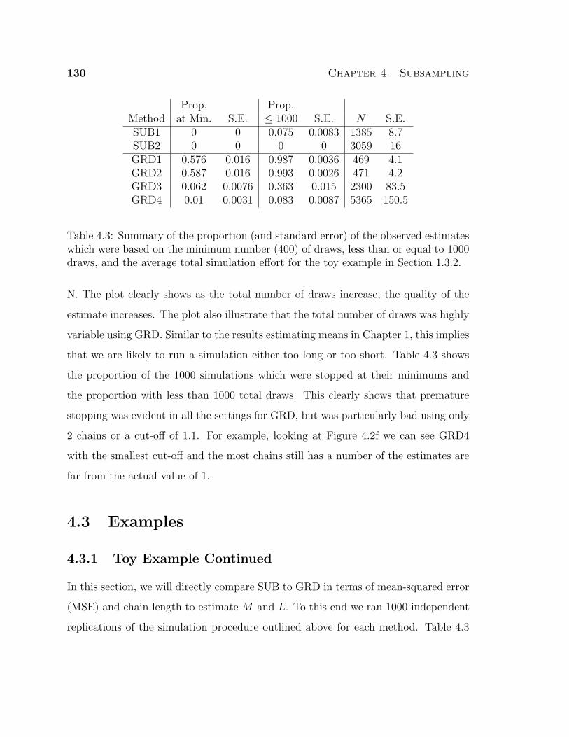
130 Chapter 4. Subsampling
Prop. Prop.Method at Min. S.E. ≤ 1000 S.E. N S.E.SUB1 0 0 0.075 0.0083 1385 8.7SUB2 0 0 0 0 3059 16GRD1 0.576 0.016 0.987 0.0036 469 4.1GRD2 0.587 0.016 0.993 0.0026 471 4.2GRD3 0.062 0.0076 0.363 0.015 2300 83.5GRD4 0.01 0.0031 0.083 0.0087 5365 150.5
Table 4.3: Summary of the proportion (and standard error) of the observed estimateswhich were based on the minimum number (400) of draws, less than or equal to 1000draws, and the average total simulation effort for the toy example in Section 1.3.2.
N. The plot clearly shows as the total number of draws increase, the quality of the
estimate increases. The plot also illustrate that the total number of draws was highly
variable using GRD. Similar to the results estimating means in Chapter 1, this implies
that we are likely to run a simulation either too long or too short. Table 4.3 shows
the proportion of the 1000 simulations which were stopped at their minimums and
the proportion with less than 1000 total draws. This clearly shows that premature
stopping was evident in all the settings for GRD, but was particularly bad using only
2 chains or a cut-off of 1.1. For example, looking at Figure 4.2f we can see GRD4
with the smallest cut-off and the most chains still has a number of the estimates are
far from the actual value of 1.
4.3 Examples
4.3.1 Toy Example Continued
In this section, we will directly compare SUB to GRD in terms of mean-squared error
(MSE) and chain length to estimate M and L. To this end we ran 1000 independent
replications of the simulation procedure outlined above for each method. Table 4.3

4.3. Examples 131
shows the percentage of time the estimates of M and L were based on both the mini-
mum and 1000 draws or less. We can see from this, that using GRD as a stopping rule
tends to stop the simulation prematurely in a significant portion of the simulations.
In our experience, the time it took to run one replication with a similar number
of draws was approximately equivalent for GRD and SUB. Therefore, we will use N ,
the total chain length, as a measure of the computational effort. Looking closely at
SUB2 and GRD4, we can see that the average number of draws are 3059 and 5365
from Table 4.3. In this case, SUB2 is using less than 60% of draws required for GRD4.
However, if we look at the quality of the estimation of M and L by comparing MSEs,
we can see that the MSEs for GRD4 are 2.5 times higher than SUB2 for estimating
M , and 2.6 times higher for estimating L (see Table 4.2). Again, it is clear the results
using SUB are superior to those using GRD. In addition, SUB allows us to work with
the actual parameter we are interested in, and provides a method to estimate the
standard errors.
However, remember for this toy example we are using a sequential sampler to
draw from the true distribution implying no burn-in is needed at all to implement
GRD method (in this specific setting). Taking this into account, we can recalculate
the estimates ignoring burn-in by using the entire chain length. For estimating M , we
can calculate the MSE of 9.99× 10⁻⁵ for GRD4 with a standard error of 7.8× 10⁻⁶,
resulting in GRD4 having a MSE 1.4 times larger than SUB2. For estimating L, the
MSE from GRD4 is 0.000473 with a standard error of 3.6× 10⁻⁵, resulting in GRD4
having an MSE 1.3 times higher than that of SUB2. This difference is not significant
based on the standard errors, but if the simulation efforts were equal, the results
would certainly be significant. Now, we can see SUB is still a superior method for
estimating M and L because of the variable total sample size related to using GRD.

132 Chapter 4. Subsampling
i y x i y x1 −0.2649 −0.0083 11 −0.3447 0.02982 −0.1552 0.4994 12 1.7768 1.66943 −2.5194 −0.1883 13 0.5059 0.53494 −0.8693 −0.3308 14 0.1383 0.93835 −0.7272 −0.7908 15 2.0452 0.29406 −3.0486 −1.9435 16 −1.9861 −0.48607 0.5511 0.0880 17 −0.3182 −0.22568 1.7590 1.9856 18 −2.3956 −1.92509 −1.0116 −0.5404 19 −2.5586 −1.014210 0.0094 0.3795 20 1.2208 0.7291
Table 4.4: Simulated data for block Gibbs example.
4.3.2 Block Gibbs Numerical Example
The goal of this example is to compare the finite sample properties obtained using
BM to SUB. To this end, we will estimate the posterior means for β, λR and λD
(denoted E(β|y), E(λR|y), and E(λD|y) respectively), calculate the MCSEs with the
two methods, and compare the results. In the case of estimating means, the estimate
from SUB is simply equal to the estimate of OBM. Additionally, we will illustrate the
use of SUB estimation of the median and first quartile for the three distributions of
interest. The medians will be denoted β(0.50), λ(0.50)R , and λ
(0.50)D . The first quartiles
will be denoted β(0.25), λ(0.25)R , and λ
(0.25)D . Application of the Markov chain CLT and
BM require geometric ergodicity and finite moment conditions. Geometric ergodicity
for the block Gibbs sampler was shown in Section 2.3.1 and, for now, we will assume
the proper moment conditions have been met for our settings to implement BM and
OBM. The theoretical justification for SUB is a future research direction.
First, we simulated the data in Table 4.4 with the model from Section 2.3.1 with
n = 20, λR = λD = 4 and covariate X ∼ N(0, I20). Then, using the block Gibbs
sampler with prior settings r1 = r2 = d1 = d2 = 4, we estimated the true value for
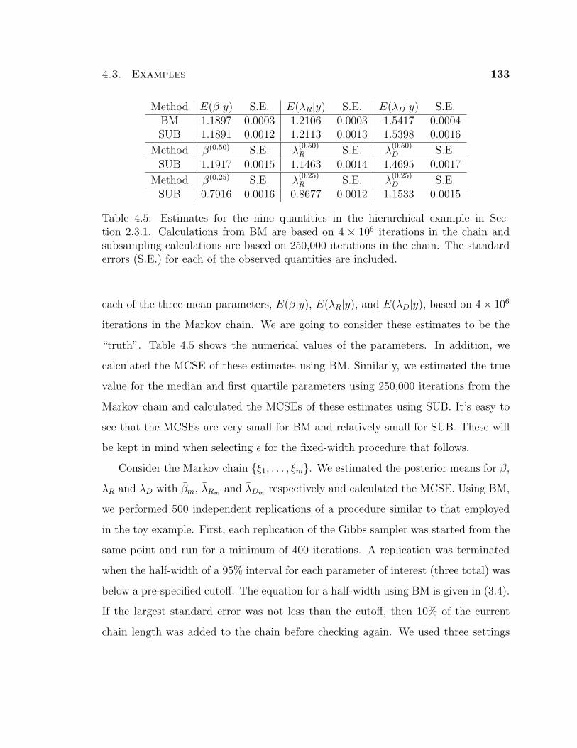
4.3. Examples 133
Method E(β|y) S.E. E(λR|y) S.E. E(λD|y) S.E.BM 1.1897 0.0003 1.2106 0.0003 1.5417 0.0004SUB 1.1891 0.0012 1.2113 0.0013 1.5398 0.0016
Method β(0.50) S.E. λ(0.50)R S.E. λ
(0.50)D S.E.
SUB 1.1917 0.0015 1.1463 0.0014 1.4695 0.0017
Method β(0.25) S.E. λ(0.25)R S.E. λ
(0.25)D S.E.
SUB 0.7916 0.0016 0.8677 0.0012 1.1533 0.0015
Table 4.5: Estimates for the nine quantities in the hierarchical example in Sec-tion 2.3.1. Calculations from BM are based on 4 × 10⁶ iterations in the chain andsubsampling calculations are based on 250,000 iterations in the chain. The standarderrors (S.E.) for each of the observed quantities are included.
each of the three mean parameters, E(β|y), E(λR|y), and E(λD|y), based on 4× 10⁶
iterations in the Markov chain. We are going to consider these estimates to be the
“truth”. Table 4.5 shows the numerical values of the parameters. In addition, we
calculated the MCSE of these estimates using BM. Similarly, we estimated the true
value for the median and first quartile parameters using 250,000 iterations from the
Markov chain and calculated the MCSEs of these estimates using SUB. It’s easy to
see that the MCSEs are very small for BM and relatively small for SUB. These will
be kept in mind when selecting ε for the fixed-width procedure that follows.
Consider the Markov chain ξ1, . . . , ξm. We estimated the posterior means for β,
λR and λD with βm, λRm and λDm respectively and calculated the MCSE. Using BM,
we performed 500 independent replications of a procedure similar to that employed
in the toy example. First, each replication of the Gibbs sampler was started from the
same point and run for a minimum of 400 iterations. A replication was terminated
when the half-width of a 95% interval for each parameter of interest (three total) was
below a pre-specified cutoff. The equation for a half-width using BM is given in (3.4).
If the largest standard error was not less than the cutoff, then 10% of the current
chain length was added to the chain before checking again. We used three settings
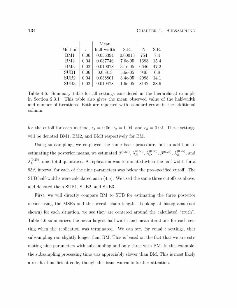
134 Chapter 4. Subsampling
MeanMethod ε half-width S.E. N S.E.BM1 0.06 0.056394 0.00013 754 7.4BM2 0.04 0.037746 7.6e-05 1683 15.4BM3 0.02 0.019078 3.1e-05 6646 47.2SUB1 0.06 0.05813 5.6e-05 946 6.8SUB2 0.04 0.038801 3.4e-05 2088 14.1SUB3 0.02 0.019478 1.6e-05 8142 38.6
Table 4.6: Summary table for all settings considered in the hierarchical examplein Section 2.3.1. This table also gives the mean observed value of the half-widthand number of iterations. Both are reported with standard errors in the additionalcolumn.
for the cutoff for each method, ε1 = 0.06, ε2 = 0.04, and ε3 = 0.02. These settings
will be denoted BM1, BM2, and BM3 respectively for BM.
Using subsampling, we employed the same basic procedure, but in addition to
estimating the posterior means, we estimated β(0.50), λ(0.50)R , λ
(0.50)D , β(0.25), λ
(0.25)R , and
λ(0.25)D , nine total quantities. A replication was terminated when the half-width for a
95% interval for each of the nine parameters was below the pre-specified cutoff. The
SUB half-widths were calculated as in (4.5). We used the same three cutoffs as above,
and denoted them SUB1, SUB2, and SUB3.
First, we will directly compare BM to SUB for estimating the three posterior
means using the MSEs and the overall chain length. Looking at histograms (not
shown) for each situation, we see they are centered around the calculated “truth”.
Table 4.6 summarizes the mean largest half-width and mean iterations for each set-
ting when the replication was terminated. We can see, for equal ε settings, that
subsampling ran slightly longer than BM. This is based on the fact that we are esti-
mating nine parameters with subsampling and only three with BM. In this example,
the subsampling processing time was appreciably slower than BM. This is most likely
a result of inefficient code, though this issue warrants further attention.
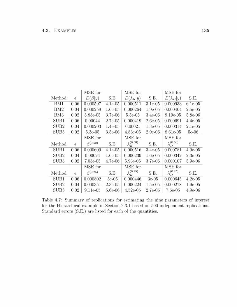
4.3. Examples 135
MSE for MSE for MSE forMethod ε E(β|y) S.E. E(λR|y) S.E. E(λD|y) S.E.BM1 0.06 0.000597 4.1e-05 0.000511 3.1e-05 0.000933 6.1e-05BM2 0.04 0.000259 1.6e-05 0.000264 1.9e-05 0.000404 2.5e-05BM3 0.02 5.83e-05 3.7e-06 5.5e-05 3.4e-06 9.19e-05 5.8e-06SUB1 0.06 0.00044 2.7e-05 0.000419 2.6e-05 0.000691 4.4e-05SUB2 0.04 0.000203 1.4e-05 0.00021 1.3e-05 0.000314 2.1e-05SUB3 0.02 5.3e-05 3.5e-06 4.83e-05 2.9e-06 8.61e-05 5e-06
MSE for MSE for MSE for
Method ε β(0.50) S.E. λ(0.50)R S.E. λ
(0.50)D S.E.
SUB1 0.06 0.000609 4.1e-05 0.000516 3.4e-05 0.000781 4.9e-05SUB2 0.04 0.00024 1.6e-05 0.000239 1.6e-05 0.000342 2.3e-05SUB3 0.02 7.03e-05 4.7e-06 5.93e-05 3.7e-06 0.000107 5.9e-06
MSE for MSE for MSE for
Method ε β(0.25) S.E. λ(0.25)R S.E. λ
(0.25)D S.E.
SUB1 0.06 0.000802 5e-05 0.000446 3e-05 0.000645 4.2e-05SUB2 0.04 0.000351 2.3e-05 0.000224 1.5e-05 0.000278 1.9e-05SUB3 0.02 9.11e-05 5.6e-06 4.52e-05 2.7e-06 7.6e-05 4.9e-06
Table 4.7: Summary of replications for estimating the nine parameters of interestfor the Hierarchical example in Section 2.3.1 based on 500 independent replications.Standard errors (S.E.) are listed for each of the quantities.
136 Chapter 4. Subsampling
Table 4.7 shows the calculated MSEs for the two different methods. Notice that
for equal settings for ε, we can see that the MSEs from BM and SUB are approxi-
mately equal. For ε1 = 0.06 and ε2 = 0.04, confidence intervals for the MSE of BM
(based on the standard error) do not contain observed MSE for SUB. However, sub-
sampling is using more iterations for equal ε because it is estimating nine quantities
rather than three. For ε3 = 0.02, the two methods are not statistically different,
based on the same reasoning. We can also compare the BM and SUB by looking
at the univariate parametric confidence intervals for each replication. For 17 of the
possible 18 combinations, the proportion of intervals containing the true parameter is
within two standard errors of the nominal value of 0.95. The exception is BM1 when
estimating E(λD|y). In this case the proportion of intervals is 0.922 with a standard
error of 0.012, so the estimate is within 2.5 standard errors of the mean. This is still
a very reasonable result considering we have 18 total combinations.
The final results using BM and SUB are very similar in this case. The benefit of
using BM is the moderately faster computational time, while SUB will enjoy a lower
asymptotic variance (because of the relationship with OBM shown in Section 3.2.3).
In the case of estimating ergodic averages, both methods enjoy checkable theoretical
conditions to ensure consistent estimators. However, as mentioned, BM will not allow
us to calculate MCSEs for estimating quantiles, this will require SUB.
Now, we will illustrate the use of subsampling for estimating univariate quantiles
of the posterior distribution. The six parameters of interest are β(0.50), λ(0.50)R , λ
(0.50)D ,
β(0.25), λ(0.25)R , and λ
(0.25)D . Again, histograms (not shown) for each situation show
nothing alarming, with the estimates centered around the true value in each case.
Table 4.7 shows the MSEs for estimating the quantile parameters are on the same
order of magnitude as those from estimating the mean parameters. Looking at the
univariate parametric confidence intervals, the observed coverage probabilities of all
18 were within two standard errors of the nominal 0.95 value. For this example, sub-
4.3. Examples 137
sampling is doing the “right” thing for estimating means and quantiles, and provides
a method to calculate MCSEs in both of these cases.
4.3.3 Discussion
As we have seen in our examples, subsampling methods seem to work well estimating
quantiles in finite sample settings. There are a number of future directions for this
research. A substantial project would be to extend the ideas for ergodic averages
in Chapter 3 to quantiles, and further to general quantities, via subsampling meth-
ods. Specifically, can the work from Politis et al. (1999) be translated into checkable
conditions for MCMC practitioners? The use of subsampling also allows calculating
non-parametric confidence intervals as in (4.2). Do these intervals ensure asymptot-
ically valid confidence intervals using fixed-width methods? Further research is also
needed in the case of establishing checkable conditions for limiting distributions for
quantities that cannot be expressed as ergodic averages. Here, the work of Carlstein
(1986) provides an excellent starting point, but more work is necessary. Finally, and
potentially most importantly, there is a culture in MCMC literature of rarely report-
ing MCSEs for the quantities of interest, including quantiles. Hence, further work is
necessary in applying the results in this thesis to important real problems seen by
practitioners.

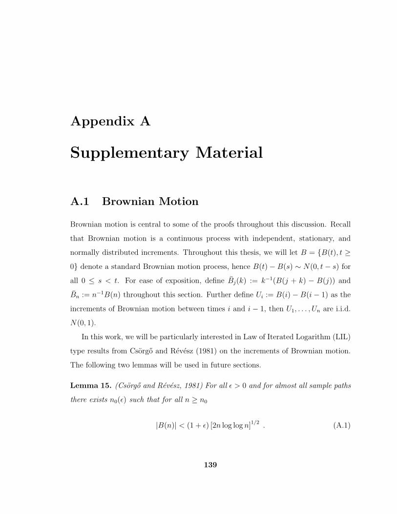
Appendix A
Supplementary Material
A.1 Brownian Motion
Brownian motion is central to some of the proofs throughout this discussion. Recall
that Brownian motion is a continuous process with independent, stationary, and
normally distributed increments. Throughout this thesis, we will let B = B(t), t ≥
0 denote a standard Brownian motion process, hence B(t)− B(s) ∼ N(0, t− s) for
all 0 ≤ s < t. For ease of exposition, define Bj(k) := k−1(B(j + k) − B(j)) and
Bn := n−1B(n) throughout this section. Further define Ui := B(i)− B(i− 1) as the
increments of Brownian motion between times i and i − 1, then U1, . . . , Un are i.i.d.
N(0, 1).
In this work, we will be particularly interested in Law of Iterated Logarithm (LIL)
type results from Csorgo and Revesz (1981) on the increments of Brownian motion.
The following two lemmas will be used in future sections.
Lemma 15. (Csorgo and Revesz, 1981) For all ε > 0 and for almost all sample paths
there exists n0(ε) such that for all n ≥ n0
|B(n)| < (1 + ε) [2n log log n]1/2 . (A.1)
139
140 Appendix A. Supplementary Material
Lemma 16. (Damerdji, 1994, Lemma 7.1.2) Suppose Assumption 2 holds, then for
all ε > 0 and for almost all sample paths, there exists n0(ε) such that for all n ≥ n0
sup0≤t≤n−bn
sup0≤s≤bn
|B(t+ s)−B(t)| < (1 + ε)
(2bn
(log
n
bn+ log log n
))1/2
.
Corollary 3. (Damerdji, 1994, p. 508) For all ε > 0 and for almost all sample paths,
there exists n0(ε) such that for all n ≥ n0
|Bj(an)| ≤√
2(1 + ε)a−1/2n
(log
n
an
+ log log n
)1/2
, (A.2)
where Bj(an) = a−1n (B((j + 1)an)−B(jan)).
A.1.1 Results for Spectral Variance
Define
σ2∗ = n−1
n−bn∑j=0
bn∑k=1
αn(k)(Bj(k)− Bn)2 .
For ease of exposition, let Ti = Ui − Bn for i = 1, . . . , n and further define
γn(s) = n−1
n−s∑t=1
UtUt+s for s = 1, . . . , n ,
fn(0) =1
2π
bn−1∑s=−(bn−1)
wn(s)γn(s) , and
dn = n−1
([bn∑l=1
∆1wn(l)
(l−1∑i=1
T 2i +
n∑i=n−bn+l+1
T 2i
)]
+ 2bn−1∑s=1
[bn−s∑l=1
∆1wn(s+ l)
(l−1∑i=1
TiTs+i +n−s∑
i=n−bn+l+1
TiTs+i
)]).
Proposition 7. Suppose Assumptions 1 and 2 hold. Further assume

A.1. Brownian Motion 141
1. there exists a constant c ≥ 1 such that∑
n(bn/n)c <∞,
2. bnn−1 log n→ 0 as n→∞,
3.
bnn−1
bn∑k=1
k |∆1wn(k)| → 0 as n→∞ ,
4. and b−1n log n stays bounded as n→∞.
Then σ2∗ → 1 as n→∞.
Proof. Proposition 3 shows,
σ2∗ = 2πfn(0)− dn .
Lemma 17 shows 2πfn(0) → 1 and Lemma 19 shows dn → 0 as n → ∞. Thus,
combining all of these yield the desired result.
Lemma 17. (Damerdji, 1991, Theorem 4.1) Suppose Assumptions 1 and 2 hold.
Further assume
1. there exists a constant c ≥ 1 such that∑
n(bn/n)c <∞, and
2. bnn−1 log n→ 0 as n→∞.
Then 2πfn(0) → 1 as n→∞ w.p.1.
Proof. This proof appears in Damerdji (1991) but it is expanded on here for clarity.
First, notice that
2πfn(0) =bn−1∑
i=−(bn−1)
wn(i)γn(i)
= γn(0) + 2bn−1∑i=1
wn(i)γn(i) .

142 Appendix A. Supplementary Material
Since U1, . . . , Un are i.i.d. N(0, 1), the classical Strong Law of Large Numbers implies
that γn(0) → 1 as n→∞ w.p.1. Hence, it suffices to show that∑bn−1
i=1 wn(i)γn(i) → 0
as n→∞ w.p.1. Then we can write for i ≤ n
γn(i) = n−1
n−i∑t=1
(Ut − Bn)(Ut+i − Bn)
= n−1
[n−i∑t=1
UtUt+i + (n− i) B2n − Bn
n−i∑t=1
(Ut + Ut+i)
]
= n−1
n−i∑t=1
UtUt+i −(
1 +i
n
)B2
n + 2B2n − n−1Bn
n−i∑t=1
(Ut + Ut+i)
= n−1
n−i∑t=1
UtUt+i −(
1 +i
n
)B2
n + Bnn−1 [B(i) + (B(n)−B(n− i))] ,
resulting in
bn−1∑i=1
wn(i)γn(i) =bn−1∑i=1
wn(i)n−1
n−i∑t=1
UtUt+i − B2n
bn−1∑i=1
wn(i)
(1 +
i
n
)
+ Bnn−1
bn−1∑i=1
wn(i) [B(i) + (B(n)−B(n− i))] . (A.3)
We will now show that each of the three terms in (A.3) tend to 0 separately.
1. Here we will show that
bn−1∑i=1
wn(i)n−1
n−i∑t=1
UtUt+i → 0 as n→∞ w.p.1. (A.4)
To this end, we will use a Borel-Cantelli argument with condition 1. It suffices
to show
E
(bn−1∑i=1
wn(i)n−1
n−i∑t=1
UtUt+i
)2a = O
(bnn
)a
, (A.5)
where the symbol “O” is the Big-Oh notation, which means there exists n0 and

A.1. Brownian Motion 143
a constant C > 0 such that∣∣∣∣∣∣E(bn−1∑
i=1
wn(i)n−1
n−i∑t=1
UtUt+i
)2c∣∣∣∣∣∣ ≤ C(bn/n)c
for all n > n0. Then since
∞∑m=1
C
(bn0+m
n0 +m
)c
<∞
using condition 1, (A.4) holds via Borel-Cantelli.
Now we will show that (A.5) holds for any positive integer c ≥ 2 using the
following lemma.
Lemma 18. (Damerdji, 1991, Corollary 4) For a sequence of i.i.d. standard
normal variables Un : n ≥ 1 where A =∑
j
∑k ajkujuk, then for c ≥ 2 we
have
E[|A− EA|2c
]≤ K(c)
(∑j
∑k
a2jk
)c
,
for some constant K(c) depending only on c.
If we then let D(n) be the n× n matrix with entries,
Di,j(n) =
n−1wn(j − i) for i < j ,
0 otherwise.
144 Appendix A. Supplementary Material
Define U := (U1, . . . , Un)T , then by construction of the matrix D(n)
A(n) = U ′D(n)U
=n∑
t=1
Ut
t−1∑i=1
n−1wn(i)Ut−i
=n−1∑i=1
n∑t=i+1
n−1wn(i)Ut−iUt
=n−1∑i=1
wn(i)n−1
n−i∑t=1
UtUt+i
=bn−1∑i=1
wn(i)n−1
n−i∑t=1
UtUt+i
where the last step results from the fact that wn(s) = 0 for all |s| ≥ bn.
Recall U1, . . . , Un are i.i.d. N(0, 1), then EA(n) = 0 since EUtUt+i = 0 for i ≥ 1,
and we can apply Lemma 18 as follows
E
(bn−1∑i=1
wn(i)n−1
n−i∑t=1
UtUt+i
)2c ≤ K(c)
(∑j
∑k
a2jk
)c
where the coefficients ajk are the elements of the matrix D(n), and K(c) is a
constant in c. Now we can see that
∑j
∑k
a2jk = n−2
bn−1∑i=1
(n− i)w2n(i) ≤ n−1
bn−1∑i=1
w2n(i) ≤ bnn
−1
and hence, we have shown the relationship in (A.5), implying the first term in
(A.3) tends to 0 as n→∞.

A.1. Brownian Motion 145
2. From Assumption 1, the fact that 1 + i/n ≤ 2, and (A.1), it follows that
0 ≤ B2n
∣∣∣∣∣bn−1∑i=1
wn(i)
(1 +
i
n
)∣∣∣∣∣ ≤ 2bnB2n
≤ 2bnn−2(1 + ε)22n log log n = 4(1 + ε)2bnn
−1 log log n→ 0 ,
as n→∞ by condition 2.
3. Again, we will use the LIL type results from Appendix A.1, specifically we will
apply Lemma 16. For 1 ≤ i ≤ bn,
|B(i) + (B(n)−B(n− i))| ≤ sup0≤s≤bn
|B(s)|+ sup0≤s≤bn
|B(n)−B(n− s)|
≤ sup0≤t≤n−bn
sup0≤s≤bn
|B(t+ s)−B(t)|
+ sup0≤s≤bn
|B(n)−B(n− s)|
≤ 2(1 + ε)
(2bn
(log
n
bn+ log log n
))1/2
.
Therefore, from Lemma 15 and the above relationship,∣∣∣∣∣Bnn−1
bn−1∑i=1
wn(i) [B(i) + (B(n)−B(n− i))]
∣∣∣∣∣≤ 4n−2(1 + ε)2 (n log log n)1/2 bn
(bn
(log
n
bn+ log log n
))1/2
= O(b3/2n n−3/2 log n) .
Hence, the above will go to 0 as a result of Assumption 2 and condition 2.

146 Appendix A. Supplementary Material
Lemma 19. (Damerdji, 1991, Proposition 4.3) Suppose Assumptions 1 and 2 hold.
If
1.
bnn−1
bn∑k=1
k |∆1wn(k)| → 0 as n→∞
2. and b−1n log n stays bounded as n→∞.
Then dn → 0 as n→∞ w.p.1.
Proof. Recall Ti = Ui − Bn for i = 1, . . . , n and
dn = n−1
([bn∑l=1
∆wn(l)
(l−1∑i=1
T 2i +
n∑i=n−bn+l+1
T 2i
)]
+ 2bn−1∑s=1
[bn−s∑l=1
∆wn(s+ l)
(l−1∑i=1
TiTs+i +n−s∑
i=n−bn+l+1
TiTs+i
)]),
We will procede similarly to the proof of Lemma 10.
1. We can bound |dn| as before
dn ≤ b−1n
(bn∑i=1
T 2i +
n∑i=n−bn+1
T 2i
)(A.6)
× n−1bn
(bn∑l=1
|∆wn(l)|+ 2bn∑
k=1
k |∆wn(k)|
). (A.7)
Again, (A.7) tends to 0 as n → ∞ by condition 1. Hence, it suffices to show
that (A.6) is bounded w.p.1.
2. The classical strong law of large numbers implies the sums∑bn
i=1 Ui and∑bn
i=1 U2i
stay bounded w.p.1. Then we can apply the same argument as above to show
the contribution from the starting effects stay bounded for dn.

A.1. Brownian Motion 147
3. Finally, we are left to show that the sums contributed from the terminating end
effects stay bounded, or b−1n
∑ni=n−bn+1 T
2i < ∞ as n → ∞. Using the same
technique as before, it suffices to show b−1n
∑ni=n−bn+1 Ui and b−1
n
∑ni=n−bn+1 U
2i
stay bounded. We have b−1n
∑ni=n−bn+1 Ui = b−1
n (B(n)−B(n− bn)), which stays
bounded by Lemma 16 and condition 2. As for b−1n
∑ni=n−bn+1 U
2i , we will use
the following strong invariance principle. Komlos et al. (1975), Komlos et al.
(1976), and Major (1976) have shown in the i.i.d. case, that if E[exp |tX1|] <∞
in a neighborhood of t = 0, then
Sn − nµ = σB(n) +O(log n) w.p.1
where the log n rate is extremely sharp. Since U1, . . . , Un are i.i.d. N(0, 1) the
sequence U21 , . . . U
2n are i.i.d. χ2
1. This implies that∣∣∣∣∣n∑
i=1
U2i − n− 2B(n)
∣∣∣∣∣ ≤ C ′ log n ,

148 Appendix A. Supplementary Material
resulting in
b−1n
∣∣∣∣∣n∑
i=n−bn+1
U2i
∣∣∣∣∣ = b−1n
∣∣∣∣∣n∑
i=1
U2i −
n−bn∑i=1
U2i
∣∣∣∣∣= b−1
n
∣∣∣∣∣(
n∑i=1
U2i − n− 2B(n)
)
−
(n−bn∑i=1
U2i − (n− bn)− 2B(n− bn)
)
+ 2 (B(n)−B(n− bn)) + bn
∣∣∣∣∣≤ b−1
n
(2C ′ log n+ (1 + ε)
(2bn
(log
n
bn+ log log n
))1/2
+ bn
)= 1 + 2C ′b−1
n log n+O((b−1
n log n)1/2)
w.p.1.
Hence, b−1n
∣∣∑ni=n−bn+1 U
2i
∣∣ stays bounded w.p.1 from condition 2.
Thus the proof is complete.
A.1.2 Results for Overlapping Batch Means
As shown previously, OBM is a special case of a SV estimator. In this section, we
will show σ2(n) → 1 w.p.1 where
σ2(n) = bnn−1
n−bn∑j=0
(Bj(k)− Bn
)2under less stringent conditions than Proposition 7.
The following lemma from Kendall and Stuart (1977) is required.
Lemma 20. If Z ∼ χ2v, then for all positive integers r there exists a constant K :=
K(r) such that E [(Z − v)2r] ≤ Kvr.

A.1. Brownian Motion 149
Proposition 8. Assume Assumption 2 and (a) there exists a constant c ≥ 1 such that∑n(bn/n)c < ∞; (b) bnn
−1 log n → 0 as n → ∞; and (c) n−3/2b2n → 0 as n → ∞,
then as n→∞, σ2(n) → 1 w.p.1.
Proof. Let wn(k) = 1− |k|/bn for |k| < bn and 0 otherwise, the modified Bartlett lag
window. Consider αn(k) := k2∆2wn(k) is a sequence of weights where ∆2wn(k) =
wn(k − 1)− 2wn(k) + wn(k + 1). Recall that
σ2(n) = bnn−1
n−bn∑j=0
(Bj(k)− Bn
)2= n−1
n−bn∑j=0
bn∑k=1
αn(k)(Bj(k)− Bn
)2.
Using this representation, Proposition 3 in Section 3.4.2 shows there exists a sequence
dn due to some end effects, such that
σ2(n) = 2πfn(0)− dn .
Lemma 17 shows 2πfn(0) → 1 as n → ∞ w.p.1. Using the modified Bartlett lag
window, Lemma 21 shows dn → 0 as n → ∞ w.p.1. Combining these yield the
desired result.
Lemma 21. Suppose Assumption 2 holds and wn(k) = 1− |k|/bn for |k| < bn and 0
otherwise. If
1. there exists a constant c ≥ 1 such that∑
n(bn/n)c <∞;
2. b−1n log n stays bounded as n→∞;
3. and n−3/2b2n → 0 as n→∞.
Then dn → 0 as n→∞ w.p.1.

150 Appendix A. Supplementary Material
Proof. Recall Ti = Ui − Bn for i = 1, . . . , n. Using the Bartlett lag window and the
definition of dn,
|dn| = n−1
∣∣∣∣∣[
bn∑l=1
∆wn(l)
(l−1∑i=1
T 2i +
n∑i=n−bn+l+1
T 2i
)]
+ 2bn−1∑s=1
[bn−s∑l=1
∆wn(s+ l)
(l−1∑i=1
TiTs+i +n−s∑
i=n−bn+l+1
TiTs+i
)]∣∣∣∣∣≤ n−1
∣∣∣∣∣bn∑l=1
b−1n
(l−1∑i=1
T 2i +
n∑i=n−bn+l+1
T 2i
)∣∣∣∣∣ (A.8)
+ n−1
∣∣∣∣∣2bn−1∑s=1
bn−s∑l=1
b−1n
(l−1∑i=1
TiTs+i +n−s∑
i=n−bn+l+1
TiTs+i
)∣∣∣∣∣ . (A.9)
We will show that (A.8) and (A.9) each tend to zero implying the desired result.
First consider (A.8),
n−1
∣∣∣∣∣bn∑l=1
b−1n
(l−1∑i=1
T 2i +
n∑i=n−bn+l+1
T 2i
)∣∣∣∣∣ ≤ n−1
∣∣∣∣∣bn∑l=1
b−1n
(bn−1∑i=1
T 2i +
n∑i=n−bn+2
T 2i
)∣∣∣∣∣= n−1
∣∣∣∣∣bn−1∑i=1
T 2i +
n∑i=n−bn+2
T 2i
∣∣∣∣∣= n−1
∣∣∣∣∣bn−1∑i=1
(Ui − Bn
)2+
n∑i=n−bn+2
(Ui − Bn
)2∣∣∣∣∣≤ n−1
∣∣∣∣∣bn−1∑i=1
U2i +
n∑i=n−bn+2
U2i
∣∣∣∣∣+ n−1
∣∣∣∣∣2Bn
(bn−1∑i=1
Ui +n∑
i=n−bn+2
Ui
)∣∣∣∣∣+ n−1
∣∣2(bn − 1)B2n
∣∣ .Now we show that each of the three terms above tend to zero.
1. Since U21 , . . . U
2n are i.i.d. χ2
1,∑bn−1
i=1 U2i +∑n
i=n−bn+2 U2i ∼ χ2
2(bn−1). By Lemma 20

A.1. Brownian Motion 151
we have
E
(bn−1∑i=1
U2i +
n∑i=n−bn+2
U2i − 2(bn − 1)
)2c ≤ K (2(bn − 1))c ,
and
E
(n−1
(bn−1∑i=1
U2i +
n∑i=n−bn+2
U2i
)− 2(bn − 1)
n
)2c ≤ K
(2(bn − 1)
n2
)c
.
By assumption there exists a constant c ≥ 1 such that∑
n(bn/n)c <∞ and
∑n
K
(2(bn − 1)
n2
)c
<∞ .
A Borel-Cantelli argument results in
(n−1
(bn−1∑i=1
U2i +
n∑i=n−bn+2
U2i
)− 2(bn − 1)
n
)2c
→ 0 w.p.1 as n→∞ .
Hence
n−1
∣∣∣∣∣bn−1∑i=1
U2i +
n∑i=n−bn+2
U2i
∣∣∣∣∣→ 0 w.p.1 as n→∞
since bn/n→ 0 as n→∞.
2. Notice
n−1
∣∣∣∣∣2Bn
(bn−1∑i=1
Ui +n∑
i=n−bn+2
Ui
)∣∣∣∣∣ ≤ 2∣∣Bn
∣∣n−1
n∑i=1
|Ui| .
By the classical strong law, n−1∑n
i=1 |Ui| →√
2/π w.p.1 since |Ui| are i.i.d.

152 Appendix A. Supplementary Material
half-normal distributions. Combining this with Lemma 15 imply
n−1
∣∣∣∣∣2Bn
(bn−1∑i=1
Ui +n∑
i=n−bn+2
Ui
)∣∣∣∣∣ ≤ 4/√πn−1/2(1 + ε) [log log n]1/2 ,
which tends to 0 as n→∞.
3. Using Lemma 15
n−1∣∣2(bn − 1)B2
n
∣∣ ≤ (1 + ε)24n−2 [log log n] (bn − 1) ,
which tends to 0 since bn/n→ 0 as n→∞.
Next, consider (A.9)
n−1
∣∣∣∣∣2bn−1∑s=1
bn−s∑l=1
b−1n
(l−1∑i=1
TiTs+i +n−s∑
i=n−bn+l+1
TiTs+i
)∣∣∣∣∣= n−1
∣∣∣∣∣2bn−1∑s=1
bn−s∑l=1
b−1n
(l−1∑i=1
(Ui − Bn
) (Us+i − Bn
)+
n−s∑i=n−bn+l+1
(Ui − Bn
) (Us+i − Bn
)) ∣∣∣∣∣≤ n−1
∣∣∣∣∣2bn−1∑s=1
bn−s∑l=1
b−1n
(l−1∑i=1
UiUs+i +n−s∑
i=n−bn+l+1
UiUs+i
)∣∣∣∣∣+ n−1
∣∣∣∣∣2bn−1∑s=1
bn−s∑l=1
Bnb−1n
(l−1∑i=1
(−Ui − Us+i) +n−s∑
i=n−bn+l+1
(−Ui − Us+i)
)∣∣∣∣∣+ n−1
∣∣∣∣∣2bn−1∑s=1
bn−s∑l=1
B2nb
−1n 2(bn − 1)
∣∣∣∣∣ .Again, we show that each of the three terms above tend to zero.

A.1. Brownian Motion 153
1. Let C(bn) be the (bn − 1)× (bn − 1) matrix with entries,
Ci,j(bn) =
2n−1b−1n (bn − i) for i > j ,
0 otherwise.
Further let D(bn) be the (bn − 1)× (bn − 1) matrix with entries,
Di,j(bn) =
2n−1b−1n j for i > j ,
0 otherwise.
Define U := (U1, . . . , Ubn−1, Un−bn+2, . . . , Un)T , then by construction
A(bn) = U ′
C 0
0 D
U
= n−12bn−1∑s=1
bn−s∑l=1
b−1n
(l−1∑i=1
UiUs+i +n−s∑
i=n−bn+l+1
UiUs+i
).
Recall U1, . . . , Ubn−1, Un−bn+2, . . . , Un are i.i.d. N(0, 1) resulting in EA(bn) = 0.
Thus, we can apply Lemma 18
E
(n−12bn−1∑s=1
bn−s∑l=1
b−1n
(l−1∑i=1
UiUs+i +n−s∑
i=n−bn+l+1
UiUs+i
))2c
≤ K(c)
(∑j
∑k
a2jk
)c
where the coefficients ajk are the elements of the matrix
C 0
0 D

154 Appendix A. Supplementary Material
and K(c) is a constant in c. Since b−1n (bn − i) < 1 for all i in C and b−1
n j < 1
for all j in D we have
∑j
∑k
a2jk ≤ n−24
bn−1∑i=1
bn−1∑j=1
12 = n−2(bn − 1)2.
Hence,
E
(n−12bn−1∑s=1
bn−s∑l=1
b−1n
(l−1∑i=1
UiUs+i +n−s∑
i=n−bn+l+1
UiUs+i
))2c
≤ K(c)
(bn − 1
n
)2c
.
Then by a Borel-Cantelli argument,
n−1
∣∣∣∣∣2bn−1∑s=1
bn−s∑l=1
b−1n
(l−1∑i=1
UiUs+i +n−s∑
i=n−bn+l+1
UiUs+i
)∣∣∣∣∣tends to 0 as n→∞ since there exists constant c ≥ 1 such that
∑n(bn/n)c <∞.
A.1. Brownian Motion 155
2. Notice
n−1
∣∣∣∣∣2bn−1∑s=1
bn−s∑l=1
Bnb−1n
(l−1∑i=1
(−Ui − Us+i) +n−s∑
i=n−bn+l+1
(−Ui − Us+i)
)∣∣∣∣∣≤ n−12
bn−1∑s=1
bn−s∑l=1
|Bn|b−1n
(l−1∑i=1
(|Ui|+ |Us+i|) +n−s∑
i=n−bn+l+1
(|Ui|+ |Us+i|)
)
≤ n−12bn−1∑s=1
bn−s∑l=1
|Bn|b−1n
(2
bn∑i=1
|Ui|+ 2n∑
i=n−bn+1
|Ui|
)
< n−12b2n|Bn|b−1n
(2
bn∑i=1
|Ui|+ 2n∑
i=n−bn+1
|Ui|
)
= n−14b2n|Bn|b−1n
(bn∑i=1
|Ui|+n∑
i=n−bn+1
|Ui|
).
Then from Lemma 15
n−14b2n|Bn|b−1n
(bn∑i=1
|Ui|+n∑
i=n−bn+1
|Ui|
)≤ n−3/24b2n(1 + ε) [2 log log n]1/2K
(A.10)
where K = b−1n
(∑bn
i=1 |Ui|+∑n
i=n−bn+1 |Ui|). If K stays bounded w.p.1 then
(A.10) tends to 0 as n→∞ since n−3/2b2n → 0 as n→∞.
Hence, it suffices to show that K stays bounded w.p.1. First notice the classical
strong law of large numbers imples b−1n
∑bn
i=1 |Ui| stays bounded w.p.1. We will
show b−1n
∑ni=n−bn+1 |Ui| stays bounded using the following strong invariance
principle. Komlos et al. (1975), Komlos et al. (1976), and Major (1976) have
shown in the i.i.d. case, that if E[exp |tX1|] < ∞ in a neighborhood of t = 0,
then
Sn − nµ = σB(n) +O(log n) w.p.1
where the log n rate is extremely sharp. We will apply this to the i.i.d. sequence
|Ui| : i ≥ 1 with a half-normal distribution. (Recall the E|Ui| =√
2/π and

156 Appendix A. Supplementary Material
Var|Ui| = 1− 2/π.) Then∣∣∣∣∣n∑
i=1
|Ui| − n√
2/π − (1− 2/π)B(n)
∣∣∣∣∣ ≤ C ′ log n ,
resulting in
b−1n
n∑i=n−bn+1
|Ui| = b−1n
∣∣∣∣∣n∑
i=1
|Ui| −n−bn∑i=1
|Ui|
∣∣∣∣∣= b−1
n
∣∣∣∣∣(
n∑i=1
|Ui| − n√
2/π − (1− 2/π)B(n)
)
−
(n−bn∑i=1
|Ui| − (n− bn)√
2/π − (1− 2/π)B(n− bn)
)
+ (1− 2/π) (B(n)−B(n− bn)) + bn√
2/π
∣∣∣∣∣≤ b−1
n
(2C ′ log n+ (1 + ε)
(2bn
(log
n
bn+ log log n
))1/2
+ bn√
2/π
)=√
2/π + 2C ′b−1n log n+O
((b−1
n log n)1/2)
w.p.1.
Hence, b−1n
∑ni=n−bn+1 |Ui| stays bounded w.p.1 since b−1
n log n stays bounded as
n→∞.
3. Using Lemma 15 we have
n−1
∣∣∣∣∣2bn−1∑s=1
bn−s∑l=1
B2nb
−1n 2(bn − 1)
∣∣∣∣∣ ≤ n−14B2nb
2n
≤ n−28(1 + ε)2 [log log n] b2n ,
which tends to 0 as n→∞ since bn/n→ 0 as n→∞.

A.1. Brownian Motion 157
A.1.3 Results for Batch Means
Recall that B = B(t), t ≥ 0 denotes a standard Brownian motion. Define
σ2BM =
bnan − 1
an−1∑k=0
(Bk − Bn)2
where Bk = b−1(B((k + 1)b)−B(kb)) for k = 0, . . . , an − 1 and Bn = n−1B(n).
Lemma 22. (Damerdji, 1994, Proposition 3.1) Assume Assumption 2 and there ex-
ists a constant c ≥ 1 such that∑
n(bn/n)c <∞, then as n→∞, σ2BM → 1 w.p.1.
Proof. Notice that
σ2BM =
bnan − 1
an−1∑k=0
(Bk − Bn)2
=an
an − 1
(1
an
an−1∑k=0
bnB2k − bnB
2n
).
Using this representation, we will the first term above goes to 1 while the second
terms tends to 0 as n→∞.
1. Properties of Brownian motion imply for all k = 0, . . . , an − 1 that Bk are i.i.d.
N(0, 1/bn) and hence bnB2k are i.i.d. χ2
1. Then∑an−1
k=0 bnB2k ∼ χ2
an. Therefore,
by Lemma 20 we have
E
(an−1∑k=0
bnB2k − an
)2c ≤ K (an)c ,
and
E
( 1
an
an−1∑k=0
bnB2k − 1
)2c ≤ K
(bnn
)c
.

158 Appendix A. Supplementary Material
Then by a Borel-Cantelli argument,
1
an
an−1∑k=0
bnB2k → 1 w.p.1 as n→∞ .
2. Similar properties of Brownian motion imply nB2n ∼ χ2
1, hence E[bnB
2n
]= bn/n.
By a Borel-Cantelli argument, if∑
n(bn/n) < ∞, then bnB2n → 0 as n → ∞
w.p.1.
More generally, we can use Lemma 20 to show
E[(nB2
n − 1)2c]≤ K ,
and therefore
E
[(bnB
2n −
bnn
)2c]≤ K
(bnn
)2c
.
Then by a Borel-Cantelli argument, bnB2n → 0 as n→∞ w.p.1.
A.1.4 Results for Mean Square Consistency
Consider the Brownian motion estimator for OBM,
σ2OBM =
nbn(n− bn)(n− bn + 1)
n−bn∑j=0
(Bj(bn)− Bn)2 .
Further define, the Brownian motion estimator for BM,
σ2BM =
bnan − 1
an−1∑k=0
(Bk − Bn)2 ,
where Bk := b−1n (B((k + 1)bn)−B(kbn + 1)) for k = 0, . . . , an − 1.

A.1. Brownian Motion 159
Lemma 23. (Damerdji, 1995, p. 285 and Lemma 2) Suppose Assumption 2 holds,
then
E[σ2
OBM
]= E
[σ2
BM
]= 1 , (A.11)
n
bnVar
[σ2
OBM
]=
4
3+ o (1) , and (A.12)
n
bnVar
[σ2
BM
]= 2 + o (1) . (A.13)
Proof. The proof for σ2BM is straight forward and is therefore omitted.
First, define Ui := B(i)−B(i− 1) as the increments of Brownian motion between
times i and i− 1 and recall that Ui are i.i.d. N(0, 1) for all i = 1, . . . , n. Notice that
Bj(bn)− Bn can be written as a linear combination of i.i.d. normal distributions for
all j = 1, . . . , n− b+ 1,
Bj(bn)− Bn =(n− b)
nb
j+b∑i=j
Ui −1
n
j−1∑i=1
Ui −1
n
n∑i=j+b+1
Ui ,
where any empty sums are defined to be zero.
Then it is easy to see the E[Bj(bn)− Bn] = 0 for all j = 1, . . . , n− b+ 1 and
Var[Bj(bn)− Bn
]= Var
[(n− b)
nb
j+b∑i=j
Ui −1
n
j−1∑i=1
Ui −1
n
n∑i=j+b+1
Ui
]
=
(n− b
nb
)2
b+n− b
n2
=n− b
bn(A.14)
for all j = 1, . . . , n− b+ 1.
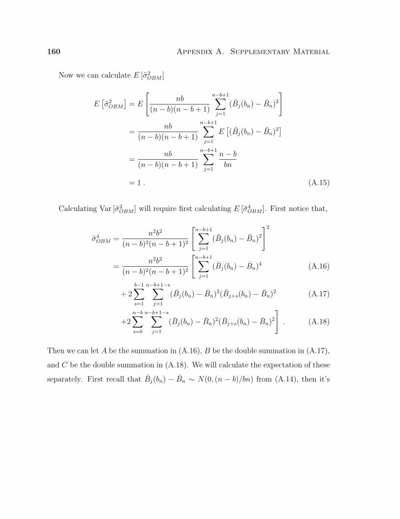
160 Appendix A. Supplementary Material
Now we can calculate E [σ2OBM ]
E[σ2
OBM
]= E
[nb
(n− b)(n− b+ 1)
n−b+1∑j=1
(Bj(bn)− Bn)2
]
=nb
(n− b)(n− b+ 1)
n−b+1∑j=1
E[(Bj(bn)− Bn)2
]=
nb
(n− b)(n− b+ 1)
n−b+1∑j=1
n− b
bn
= 1 . (A.15)
Calculating Var [σ2OBM ] will require first calculating E [σ4
OBM ]. First notice that,
σ4OBM =
n2b2
(n− b)2(n− b+ 1)2
[n−b+1∑
j=1
(Bj(bn)− Bn)2
]2
=n2b2
(n− b)2(n− b+ 1)2
[n−b+1∑
j=1
(Bj(bn)− Bn)4 (A.16)
+ 2b−1∑s=1
n−b+1−s∑j=1
(Bj(bn)− Bn)2(Bj+s(bn)− Bn)2 (A.17)
+2n−b∑s=b
n−b+1−s∑j=1
(Bj(bn)− Bn)2(Bj+s(bn)− Bn)2
]. (A.18)
Then we can let A be the summation in (A.16), B be the double summation in (A.17),
and C be the double summation in (A.18). We will calculate the expectation of these
separately. First recall that Bj(bn) − Bn ∼ N(0, (n − b)/bn) from (A.14), then it’s

A.1. Brownian Motion 161
easy to see
EA =n−b+1∑
j=1
E[(Bj(bn)− Bn)4
]=
n−b+1∑j=1
3
(n− b
bn
)2
= 3(n− b+ 1)
(n− b
bn
)2
. (A.19)
We will calculate EB by first calculating
E[(Bj(bn)− Bn)2(Bj+s(bn)− Bn)2
]= E
[Z2
1Z22
]where Z1 := (Bj(bn)− Bn) and Z2 := (Bj+s(bn)− Bn) for all j = 1, . . . , n− b+ 1− s
and s = 1, . . . , b − 1. Notice that both Z1 and Z2 are linear combinations of i.i.d.
standard normal random variables. We will calculate the joint normal distribution of
Z := (Z1, Z2)T . Recall that U := (U1, . . . , Un)T , then
U ∼ N (0, In) ,
and if D is a m× n matrix, then the random vector Z = DU is jointly normal with
Z ∼ N(0, DDT
).
Then we can calculate the distribution of Z as Z1
Z2
∼ N
0
0
,Σ
,

162 Appendix A. Supplementary Material
where
Σ =
n−bbn
(b− s)(
n−bnb
)2 − 2sn
(n−bnb
)+ n−b−s
n2
(b− s)(
n−bnb
)2 − 2sn
(n−bnb
)+ n−b−s
n2n−bbn
=
n−bbn
nb−ns−b2
nb2
nb−ns−b2
nb2n−bbn
.
To calculate the desired expectation, we will iterate the expectation. To this end, we
will need to calculate the conditional distribution of Z1|Z2 and the marginal distri-
bution of Z2. Recall that if X1
X2
∼ N
µ1
µ2
,
Σ11 Σ12
Σ21 Σ22
,
and Σ22 is non-singular, then the conditional distribution of X1|X2 is
X1|X2 ∼ N(µ1 + Σ12Σ
−122 (X2 − µ2) ,Σ11 − Σ12Σ
−122 Σ21
).
In our case, n−bbn
is clearly non-singular since b < n, and we can calculate the condi-
tional distribution of Z1|Z2 and the marginal distribution of Z2 as
Z1|Z2 ∼ N
(b(n− b)− ns
b(n− b)Z2,
2bs(n− b)− ns2
b3(n− b)
)Z2 ∼ N
(0,n− b
bn
).
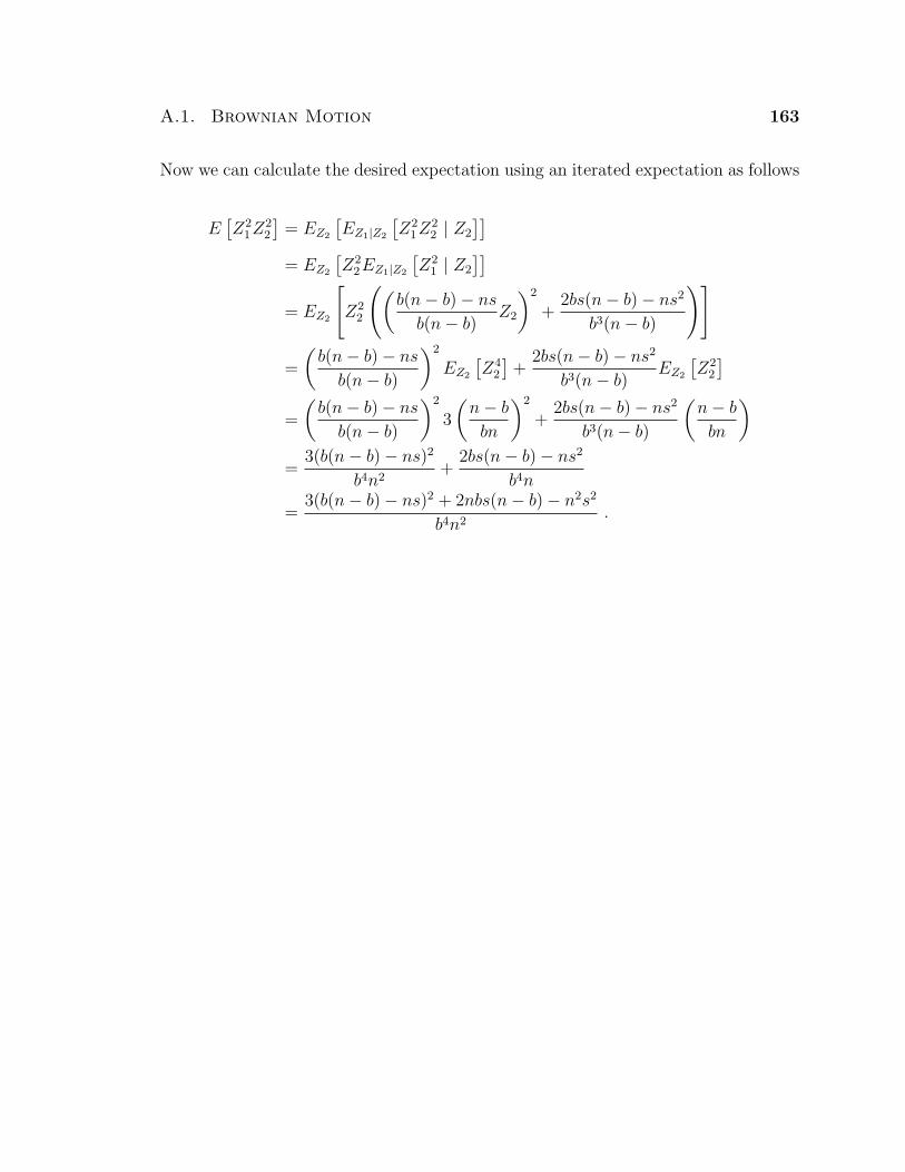
A.1. Brownian Motion 163
Now we can calculate the desired expectation using an iterated expectation as follows
E[Z2
1Z22
]= EZ2
[EZ1|Z2
[Z2
1Z22 | Z2
]]= EZ2
[Z2
2EZ1|Z2
[Z2
1 | Z2
]]= EZ2
[Z2
2
((b(n− b)− ns
b(n− b)Z2
)2
+2bs(n− b)− ns2
b3(n− b)
)]
=
(b(n− b)− ns
b(n− b)
)2
EZ2
[Z4
2
]+
2bs(n− b)− ns2
b3(n− b)EZ2
[Z2
2
]=
(b(n− b)− ns
b(n− b)
)2
3
(n− b
bn
)2
+2bs(n− b)− ns2
b3(n− b)
(n− b
bn
)=
3(b(n− b)− ns)2
b4n2+
2bs(n− b)− ns2
b4n
=3(b(n− b)− ns)2 + 2nbs(n− b)− n2s2
b4n2.

164 Appendix A. Supplementary Material
Next, we can calculate
EB = E
[b−1∑s=1
n−b+1−s∑j=1
(Bj(bn)− Bn)2(Bj+s(bn)− Bn)2
]
=b−1∑s=1
n−b+1−s∑j=1
E[(Bj(bn)− Bn)2(Bj+s(bn)− Bn)2
]=
b−1∑s=1
n−b+1−s∑j=1
E[Z2
1Z22
]=
b−1∑s=1
n−b+1−s∑j=1
[3(b(n− b)− ns)2 + 2nbs(n− b)− n2s2
b4n2
]
=b−1∑s=1
(n− b+ 1− s)
[3(b(n− b)− ns)2 + 2nbs(n− b)− n2s2
b4n2
]
=1
b4n2
b−1∑s=1
(n− b+ 1− s)[3b2(n− b)2 − 4nbs(n− b) + 2n2s2
]=
1
b4n2
[3b2(n− b)2(n− b+ 1)(b− 1)− 4nb(n− b)(n− b+ 1)
b−1∑s=1
s
+ 2n2(n− b+ 1)b−1∑s=1
s2 − 3b2(n− b)2
b−1∑s=1
s
+ 4nb(n− b)b−1∑s=1
s2 − 2n2
b−1∑s=1
s3
].
Then by mathematical fact
b−1∑s=1
s =(b− 1)b
2,
b−1∑s=1
s2 =(b− 1)b(2b− 1)
6, and
b−1∑s=1
s3 =(b− 1)2b2
4.

A.1. Brownian Motion 165
Resulting in
EB =1
b4n2
[3b2(n− b)2(n− b+ 1)(b− 1)− 4nb(n− b)(n− b+ 1)
b−1∑s=1
s
+ 2n2(n− b+ 1)b−1∑s=1
s2 − 3b2(n− b)2
b−1∑s=1
s
+ 4nb(n− b)b−1∑s=1
s2 − 2n2
b−1∑s=1
s3
]
=1
b4n2
[3b2(n− b)2(n− b+ 1)(b− 1)− 4nb(n− b)(n− b+ 1)
(b− 1)b
2
+ 2n2(n− b+ 1)(b− 1)b(2b− 1)
6− 3b2(n− b)2 (b− 1)b
2
+ 4nb(n− b)(b− 1)b(2b− 1)
6− 2n2 (b− 1)2b2
4
]=
1
6b3n2
[18b(n− b)2(n− b+ 1)(b− 1)− 12nb(n− b)(n− b+ 1)(b− 1)
+ 2n2(n− b+ 1)(b− 1)(2b− 1)− 9b2(n− b)2(b− 1)
+ 4nb(n− b)(b− 1)(2b− 1)− 3n2b(b− 1)2].
Now we are going to rearrange terms from 2 parts of the above expression
2n2(n− b+ 1)(b− 1)(2b− 1)− 3n2b(b− 1)2
= 2n3(b− 1)(2b− 1)− 2n2(b− 1)2(2b− 1)− 3n2b(b− 1)2
= 2n3(b− 1)(2b− 1)− n2(b− 1)2(7b− 2) .

166 Appendix A. Supplementary Material
We will also rearrange the 4 remaining terms,
18b(n− b)2(n− b + 1)(b− 1)− 12nb(n− b)(n− b + 1)(b− 1)
− 9b2(n− b)2(b− 1) + 4nb(n− b)(b− 1)(2b− 1)
= 18b(n− b)(n− b + 1)2(b− 1)− 18b(n− b)(n− b + 1)(b− 1)
− 12b(n− b)(n− b + 1)2(b− 1)− 12b(n− b)(n− b + 1)(b− 1)2
− 9b2(n− b)2(b− 1) + 4nb(n− b)(b− 1)(2b− 1)
= 6b(n− b)(n− b + 1)2(b− 1)− 18b(n− b)(n− b + 1)(b− 1)
− 12b(n− b)(n− b + 1)(b− 1)2
− 9b2(n− b)2(b− 1) + 4nb(n− b)(b− 1)(2b− 1)
= 6b(n− b)(n− b + 1)2(b− 1)− 18b(n− b)(n− b + 1)(b− 1)
− 12b2(n− b)(n− b + 1)(b− 1) + 12b(n− b)(n− b + 1)(b− 1)
− 9b2(n− b)(n− b + 1)(b− 1) + 9b2(n− b)(b− 1)
+ 8b2(n− b)(n− b + 1)(b− 1) + 8b2(n− b)(b− 1)2 − 4nb(n− b)(b− 1)
= 6b(n− b)(n− b + 1)2(b− 1)− 13b2(n− b)(n− b + 1)(b− 1)
+ 9b2(n− b)(b− 1) + 8b2(n− b)(b− 1)2
− 4nb(n− b)(b− 1)− 6b(n− b)(n− b + 1)(b− 1)
= 6b(n− b)(n− b + 1)2(b− 1)− 13b2(n− b)(n− b + 1)(b− 1)
+ 9b2(n− b)(b− 1) + 8b2(n− b)(b− 1)2
− 4b(n− b)2(b− 1)− 4b2(n− b)(b− 1)
− 6b(n− b)2(b− 1)− 6b(n− b)(b− 1)
= 6b(n− b)(n− b + 1)2(b− 1)− 13b2(n− b)(n− b + 1)(b− 1)
− 10b(n− b)2(b− 1) + b(n− b)(b− 1) [9b + 8b(b− 1)− 4b− 6]
= 6b(n− b)(n− b + 1)2(b− 1)− 13b2(n− b)(n− b + 1)(b− 1)
− 10b(n− b)2(b− 1) + b(n− b)(b− 1)[8b2 − 3b− 6
].

A.1. Brownian Motion 167
Then we can present the result as in Damerdji (1995),
EB =1
6b3n2
[18b(n− b)2(n− b+ 1)(b− 1)− 12nb(n− b)(n− b+ 1)(b− 1)
+ 2n2(n− b+ 1)(b− 1)(2b− 1)− 9b2(n− b)2(b− 1)
+ 4nb(n− b)(b− 1)(2b− 1)− 3n2b(b− 1)2]
=1
6b3n2
[6b(n− b)(n− b+ 1)2(b− 1)− 13b2(n− b)(n− b+ 1)(b− 1)
− 10b(n− b)2(b− 1) + b(n− b)(b− 1)[8b2 − 3b− 6
]+2n3(b− 1)(2b− 1)− n2(b− 1)2(7b− 2)
]. (A.20)
Similar to the previous expectation, we will calculate the EC by first calculating
E[(Bj(bn)− Bn)2(Bj+s(bn)− Bn)2
]= E
[Z2
1Z22
]where Z1 = (Bj(bn)−Bn) and Z2 = (Bj+s(bn)−Bn) for all j = 1, . . . , n−b+1−s and
s = b, . . . , n−b. Notice that both Z1 and Z2 are linear combinations of i.i.d. standard
normal random variables. We can again calculate the joint normal distribution of Z1
and Z − 2 as Z1
Z2
∼ N
0
0
,
n−bbn
− 1n
− 1n
n−bbn
,
resulting in the conditional distribution of Z1|Z2 and the marginal distribution of Z2
as
Z1|Z2 ∼ N
(−bn− b
Z2,
[n− b
bn− bn
n2(n− b)
])Z2 ∼ N
(0,n− b
bn
).

168 Appendix A. Supplementary Material
Then we can calculate the desired expectation using an iterated expectation as follows
E[Z2
1Z22
]= EZ2
[EZ1|Z2
[Z2
1Z22 | Z2
]]= EZ2
[Z2
2EZ1|Z2
[Z2
1 | Z2
]]= EZ2
[Z2
2
((−bn− b
Z2
)2
+
[n− b
bn− bn
n2(n− b)
])]
=
(−bn− b
)2
EZ2
[Z4
2
]+
[n− b
bn− bn
n2(n− b)
]EZ2
[Z2
2
]=
(−bn− b
)2
3
(n− b
bn
)2
+
[n− b
bn− bn
n2(n− b)
]n− b
bn
=2
n2+
(n− b
bn
)2
Finally, we can calculate the EC,
EC = E
[n−b∑s=b
n−b+1−s∑j=1
(Bj(bn)− Bn)2(Bj+s(bn)− Bn)2
]
=n−b∑s=b
n−b+1−s∑j=1
E[(Bj(bn)− Bn)2(Bj+s(bn)− Bn)2
]=
n−b∑s=b
n−b+1−s∑j=1
E[Z2
1Z22
]=
n−b∑s=b
n−b+1−s∑j=1
[2
n2+
(n− b
bn
)2]
=
[2
n2+
(n− b
bn
)2]
n−b∑s=b
(n− b+ 1− s)
=
[2
n2+
(n− b
bn
)2][
(n− 2b+ 1)(n− b+ 1)−n−b∑s=b
s
]
=
[2
n2+
(n− b
bn
)2] [
(n− 2b+ 1)(n− b+ 1)− n(n− 2b+ 1)
2
].

A.1. Brownian Motion 169
We can further factor the second part into a more desireable form
[(n− 2b+ 1)(n− b+ 1)− n(n− 2b+ 1)
2
]=
[(n− b+ 1)2 − b(n− b+ 1)− n(n− b+ 1)
2+nb
2
]=
[(n− b+ 1)2 − b(n− b+ 1)− (n− b+ 1)2
2− (b− 1)(n− b+ 1)
2+nb
2
]=
[(n− b+ 1)2
2− b(n− b+ 1)− (b− 1)(n− b+ 1)
2+nb
2
]=
[(n− b+ 1)2
2− (3b− 1)(n− b+ 1) + b(n− b+ 1) + b(b− 1)
2
]=
1
2
[(n− b+ 1)2 − (2b− 1)(n− b+ 1) + b(b− 1)
].
Then we can plug in the above result to get
EC =
[2
n2+
(n− b
bn
)2] [
(n− 2b+ 1)(n− b+ 1)− n(n− 2b+ 1)
2
]
=1
2
[2
n2+
(n− b
bn
)2] [
(n− b+ 1)2 − (2b− 1)(n− b+ 1) + b(b− 1)]. (A.21)

170 Appendix A. Supplementary Material
Combining the results from (A.19), (A.20), and (A.21), we get
E[σ4
OBM
]=
n2b2
(n− b)2(n− b + 1)2[EA + 2EB + 2EC]
=n2b2
(n− b)2(n− b + 1)2
[3(n− b + 1)
(n− b
bn
)2
+1
3b3n2
[6b(n− b)(n− b + 1)2(b− 1)− 13b2(n− b)(n− b + 1)(b− 1)
− 10b(n− b)2(b− 1) + b(n− b)(b− 1)[8b2 − 3b− 6
]+2n3(b− 1)(2b− 1)− n2(b− 1)2(7b− 2)
]+
[2n2
+(
n− b
bn
)2] [
(n− b + 1)2 − (2b− 1)(n− b + 1) + b(b− 1)]]
= 1 +2n3(b− 1)(2b− 1)
3m(n− b)2(n− b + 1)2+
2(b− 1)(n− b)
− 2(b− 2)(n− b + 1)
+(b− 1)(3b− 10)3(n− b + 1)2
+2b2
(n− b)2− 13b(b− 1)
3(n− b)(n− b + 1)+
(b− 1)[8b2 − 3b− 6
]3(n− b)(n− b + 1)2
− 2b2(2b− 1)(n− b)2(n− b + 1)
− n2(b− 1)2(7b− 2)3b(n− b)2(n− b + 1)2
+2b3(b− 1)
(n− b)2(n− b + 1)2,
and so
E[σ4
OBM
]= 1 +
4b
3n+ o
(b
n
). (A.22)
The “little-o” notation can be alternatively written as for all ε > 0, there exists a
n0(ε) such that ∣∣∣∣E [σ4OBM
]− 1− 4b
3n
∣∣∣∣ < ε
∣∣∣∣ bn∣∣∣∣ ,
for all n > n0(ε).

A.1. Brownian Motion 171
Finally, we can calculate Var [σ2OBM ] from (A.15) and (A.22)
Var[σ2
OBM
]= E
[σ4
OBM
]−(E[σ2
OBM
])2= 1 +
4b
3n+ o
(b
n
)− 12
=4b
3n+ o
(b
n
).

References
Alexopoulos, C. and Goldsman, D. (2004). To batch or not to batch? ACM Trans.
Model. Comput. Simul., 14(1):76–114.
Anderson, T. W. (1984). An Introduction to Multivariate Statistical Analysis. John
Wiley & Sons.
Anderson, T. W. (1994). The Statistical Analysis of Time Series (Classics Edition).
Wiley-Interscience.
Athreya, K. B., Doss, H., and Sethuraman, J. (1996). On the convergence of the
Markov chain simulation method. The Annals of Statistics, 24(1):69–100.
Bednorz, W. and Latuszynski, K. (2007). A few remarks on ‘Fixed-width output
analysis for Markov chain Monte Carlo’ by Jones et al. Journal of the American
Statistical Association (to appear).
Bertail, P. and Clemencon, S. (2006). Regenerative block-bootstrap for Markov
chains. Bernoulli, 12:689–712.
Bratley, P., Fox, B. L., and Schrage, L. E. (1987). A Guide to Simulation. Springer–
Verlag, New York.
Brooks, S. P. and Gelman, A. (1998). General methods for monitoring convergence
of iterative simulations. Journal of Computational and Graphical Statistics, 7:434–
455.
Buhlmann, P. (2002). Bootstraps for time series. Statistical Science, 17:52–72.
Carlstein, E. (1986). Asymptotic normality for a general statistic from a stationary
sequence. The Annals of Probability, 14:1371–1379.
173
174 References
Chen, M.-H. and Shao, Q.-M. (2001). Propriety of posterior distribution for dichoto-
mous quantal response models. Proceedings of the American Mathematical Society,
129(1):293–302.
Chen, M.-H., Shao, Q.-M., and Ibrahim, J. G. (2000). Monte Carlo Methods in
Bayesian Computation. Springer-Verlag Inc.
Chien, C.-H., Goldsman, D., and Melamed, B. (1997). Large-sample results for batch
means. Management Science, 43:1288–1295.
Christensen, O. F., Moller, J., and Waagepetersen, R. P. (2001). Geometric ergodicity
of Metropolis-Hastings algorithms for conditional simulation in generalized linear
mixed models. Methodology and Computing in Applied Probability, 3:309–327.
Cowles, M. K. and Carlin, B. P. (1996). Markov chain Monte Carlo convergence
diagnostics: A comparative review. Journal of the American Statistical Association,
91:883–904.
Cowles, M. K., Roberts, G. O., and Rosenthal, J. S. (1999). Possible biases induced by
MCMC convergence diagnostics. Journal of Statistical Computing and Simulation,
64:87–104.
Csaki, E. and Csorgo, M. (1995). On additive functionals of Markov chains. Journal
of Theoretical Probability, 8:905–919.
Csorgo, M. and Revesz, P. (1981). Strong Approximations in Probability and Statis-
tics. Academic Press.
Damerdji, H. (1991). Strong consistency and other properties of the spectral variance
estimator. Management Science, 37:1424–1440.
Damerdji, H. (1994). Strong consistency of the variance estimator in steady-state
simulation output analysis. Mathematics of Operations Research, 19:494–512.
Damerdji, H. (1995). Mean-square consistency of the variance estimator in steady-
state simulation output analysis. Operations Research, 43:282–291.
References 175
Datta, S. and McCormick, W. P. (1993). Regeneration-based bootstrap for Markov
chains. The Canadian Journal of Statistics / La Revue Canadienne de Statistique,
21:181–193.
Davison, A. C. and Hinkley, D. V. (1997). Bootstrap Methods and Their Application.
Cambridge University Press.
Douc, R., Fort, G., Moulines, E., and Soulier, P. (2004). Practical drift conditions
for subgeometric rates of convergence. The Annals of Applied Probability, 14:1353–
1377.
Doukhan, P., Massart, P., and Rio, E. (1994). The functional central limit theorem
for strongly mixing processes. Annales de l’Institut Henri Poincare, Section B,
Calcul des Probabilities et Statistique, 30:63–82.
Efron, B. and Tibshirani, R. (1993). An Introduction to the Bootstrap. Chapman &
Hall Ltd.
Finley, A. O., Banerjee, S., and Carlin, B. P. (2007). spBayes: an R package for
univariate and multivariate hierarchical point-referenced spatial models. Journal
of Statistical Software, 19.
Fishman, G. S. (1996). Monte Carlo: Concepts, Algorithms, and Applications.
Springer, New York.
Flegal, J. M., Haran, M., and Jones, G. L. (2008). Markov chain Monte Carlo: Can
we trust the third significant figure? Statistical Science (to appear).
Flegal, J. M. and Jones, G. L. (2008). Asymptotic properties for batch means and
spectral variance estimators in Markov chain Monte Carlo. Technical report, Uni-
versity of Minnesota, School of Statistics.
Fort, G. and Moulines, E. (2000). V-subgeometric ergodicity for a Hastings-Metropolis
algorithm. Statistics and Probability Letters, 49:401–410.
Fort, G. and Moulines, E. (2003). Polynomial ergodicity of Markov transition kernels.
Stochastic Processes and their Applications, 103:57–99.
176 References
Gelman, A., Carlin, J. B., Stern, H. S., and Rubin, D. B. (2004). Bayesian Data
Analysis. Chapman & Hall/CRC, Boca Raton, second edition.
Gelman, A. and Rubin, D. B. (1992). Inference from iterative simulation using mul-
tiple sequences. Statistical Science, 7:457–472.
Geyer, C. J. (1992). Practical Markov chain Monte Carlo (with discussion). Statistical
Science, 7:473–511.
Geyer, C. J. (1999). Likelihood inference for spatial point processes. In Barndorff-
Nielsen, O. E., Kendall, W. S., and van Lieshout, M. N. M., editors, Stochastic
Geometry: Likelihood and Computation, pages 79–140. Chapman & Hall/CRC,
Boca Raton.
Geyer, C. J. and Thompson, E. A. (1995). Annealing Markov chain Monte Carlo with
applications to ancestral inference. Journal of the American Statistical Association,
90:909–920.
Glynn, P. W. and Iglehart, D. L. (1990). Simulation output analysis using standard-
ized time series. Mathematics of Operations Research, 15:1–16.
Glynn, P. W. and Whitt, W. (1991). Estimating the asymptotic variance with batch
means. Operations Research Letters, 10:431–435.
Glynn, P. W. and Whitt, W. (1992). The asymptotic validity of sequential stopping
rules for stochastic simulations. The Annals of Applied Probability, 2:180–198.
Haran, M., Bhat, K., Molineros, J., and De Wolf, E. (2008). Estimating the risk of
a crop epidemic from coincident spatiotemporal processes. Technical report, The
Pennsylvania State University, Department of Statistics.
Hoaglin, D. C. and Andrews, D. F. (1975). The reporting of computation-based
results in statistics. The American Statistician, 29:122–126.
Hobert, J. P. and Geyer, C. J. (1998). Geometric ergodicity of Gibbs and block Gibbs
samplers for a hierarchical random effects model. Journal of Multivariate Analysis,
67:414–430.
References 177
Hobert, J. P., Jones, G. L., Presnell, B., and Rosenthal, J. S. (2002). On the ap-
plicability of regenerative simulation in Markov chain Monte Carlo. Biometrika,
89:731–743.
Ibragimov, I. A. and Linnik, Y. V. (1971). Independent and Stationary Sequences of
Random Variables. Walters-Noordhoff, The Netherlands.
Ihaka, R. and Gentleman, R. (1996). R: A language for data analysis and graphics.
Journal of Computational and Graphical Statistics, 5:299–314.
Jarner, S. F. and Hansen, E. (2000). Geometric ergodicity of Metropolis algorithms.
Stochastic Processes and Their Applications, 85:341–361.
Jarner, S. F. and Roberts, G. O. (2002). Polynomial convergence rates of Markov
chains. Annals of Applied Probability, 12:224–247.
Johnson, A. A. and Jones, G. L. (2008). Gibbs sampling for a Bayesian hierarchical
version of the general linear mixed model. Technical report, University of Min-
nesota, School of Statistics.
Jones, G. L. (2004). On the Markov chain central limit theorem. Probability Surveys,
1:299–320.
Jones, G. L., Haran, M., Caffo, B. S., and Neath, R. (2006). Fixed-width output anal-
ysis for Markov chain Monte Carlo. Journal of the American Statistical Association,
101:1537–1547.
Jones, G. L. and Hobert, J. P. (2001). Honest exploration of intractable probability
distributions via Markov chain Monte Carlo. Statistical Science, 16:312–334.
Jones, G. L. and Hobert, J. P. (2004). Sufficient burn-in for Gibbs samplers for a
hierarchical random effects model. The Annals of Statistics, 32:784–817.
Kendall, M. G. and Stuart, A. (1977). The Advanced Theory of Statistics. Vol. I:
Distribution Theory (4th Ed); Vol. 2: Inference and Relationship (3rd Ed). Charles
Griffin & Co.
178 References
Komlos, J., Major, P., and Tusnady, G. (1975). An approximation of partial sums
of independent RVs and the sample DF. I (Ref: 76V34 p33-58). Zeitschrift fur
Wahrscheinlichkeitstheorie und verwandte Gebiete, 32:111–131.
Komlos, J., Major, P., and Tusnady, G. (1976). An approximation of partial sums of
independent RV’s, and the sample DF. II (Ref: 75V32 p111-131). Zeitschrift fur
Wahrscheinlichkeitstheorie und verwandte Gebiete, 34:33–58.
Latuszynski, K. (2008). MCMC (e-a)-approximation under drift condition with appli-
cation to Gibbs samplers for a hierarchical random effects model. Technical report,
Warsaw School of Economics, Department of Mathematical Statistics.
L’Ecuyer, P., Simard, R., Chen, E. J., and Kelton, W. D. (2002). An objected-oriented
random-number package with many long streams and substreams. Operations Re-
search, 50:1073–1075.
Liu, J. S. (2001). Monte Carlo Strategies in Scientific Computing. Springer, New
York.
Liu, J. S. and Wu, Y. N. (1999). Parameter expansion for data augmentation. Journal
of the American Statistical Association, 94:1264–1274.
Major, P. (1976). The approximation of partial sums of independent RV’s. Zeitschrift
fur Wahrscheinlichkeitstheorie und verwandte Gebiete, 35:213–220.
Marchev, D. and Hobert, J. P. (2004). Geometric ergodicity of van Dyk and Meng’s
algorithm for the multivariate Student’s t model. Journal of the American Statis-
tical Association, 99:228–238.
Marinari, E. and Parisi, G. (1992). Simulated tempering: A new Monte Carlo scheme.
Europhysics Letters, 19:451–458.
Meketon, M. S. and Schmeiser, B. (1984). Overlapping batch means: something for
nothing? In WSC ’84: Proceedings of the 16th conference on Winter simulation,
pages 226–230, Piscataway, NJ, USA. IEEE Press.
Mengersen, K. and Tweedie, R. L. (1996). Rates of convergence of the Hastings and
Metropolis algorithms. The Annals of Statistics, 24:101–121.
References 179
Meyn, S. P. and Tweedie, R. L. (1993). Markov Chains and Stochastic Stability.
Springer-Verlag, London.
Meyn, S. P. and Tweedie, R. L. (1994). Computable bounds for geometric convergence
rates of Markov chains. The Annals of Applied Probability, 4:981–1011.
Mira, A. and Tierney, L. (2002). Efficiency and convergence properties of slice sam-
plers. Scandinavian Journal of Statistics, 29:1–12.
Mykland, P., Tierney, L., and Yu, B. (1995). Regeneration in Markov chain samplers.
Journal of the American Statistical Association, 90:233–241.
Nummelin, E. (1984). General Irreducible Markov Chains and Non-negative Opera-
tors. Cambridge University Press, London.
Nummelin, E. and Tuominen, P. (1982). Geometric ergodicity of Harris recurrent
Markov chains with applications to renewal theory. Stochastic Processes and their
Applications, 12:187–202.
Philipp, W. and Stout, W. (1975). Almost sure invariance principles for partial sums
of weakly dependent random variables. Memoirs of the American Mathematical
Society, 2:1–140.
Politis, D. N. (2003). The impact of bootstrap methods on time series analysis.
Statistical Science, 18:219–230.
Politis, D. N., Romano, J. P., and Wolf, M. (1999). Subsampling. Springer-Verlag
Inc.
Priestley, M. B. (1981). Spectral Analysis and Time Series. (Vol. 1): Univariate
Series. Academic Press.
Robert, C. P. (1995). Convergence control methods for Markov chain Monte Carlo
algorithms. Statistical Science, 10:231–253.
Robert, C. P. and Casella, G. (1999). Monte Carlo Statistical Methods. Springer,
New York.
180 References
Roberts, G. O. (1996). Markov chain concepts related to sampling algorithms. In
Gilks, W. R., Richardson, S., and Spiegelhalter, D. J. E., editors, Markov Chain
Monte Carlo in Practice, pages 45–57. Chapman & Hall, Boca Raton.
Roberts, G. O. and Polson, N. G. (1994). On the geometric convergence of the Gibbs
sampler. Journal of the Royal Statistical Society, Series B, 56:377–384.
Roberts, G. O. and Rosenthal, J. S. (1997). Geometric ergodicity and hybrid Markov
chains. Electronic Communications in Probability, 2:13–25.
Roberts, G. O. and Rosenthal, J. S. (1999). Convergence of slice sampler Markov
chains. Journal of the Royal Statistical Society, Series B, 61:643–660.
Roberts, G. O. and Rosenthal, J. S. (2004). General state space Markov chains and
MCMC algorithms. Probability Surveys, 1:20–71.
Roberts, G. O. and Tweedie, R. L. (1999). Bounds on regeneration times and con-
vergence rates for Markov chains. Stochastic Processes and their Applications,
80:211–229. Corrigendum (2001) 91:337-338.
Roberts, G. O. and Tweedie, R. L. (2001). Corrigendum to “Bounds on regeneration
times and convergence rates for Markov chains”. Stochastic Processes and their
Applications, 91:337–338.
Rosenthal, J. S. (1995). Minorization conditions and convergence rates for Markov
chain Monte Carlo. Journal of the American Statistical Association, 90:558–566.
Rosenthal, J. S. (1996). Analysis of the Gibbs sampler for a model related to James-
Stein estimators. Statistics and Computing, 6:269–275.
Roy, V. and Hobert, J. P. (2007). Convergence rates and asymptotic standard errors
for Markov chain Monte Carlo algorithms for Bayesian probit regression. Journal
of the Royal Statistical Society, Series B: Statistical Methodology, 69(4):607–623.
Song, W. T. and Schmeiser, B. W. (1995). Optimal mean-squared-error batch sizes.
Management Science, 41:110–123.
Tierney, L. (1994). Markov chains for exploring posterior distributions (with discus-
sion). The Annals of Statistics, 22:1701–1762.
References 181
van Dyk, D. A. and Meng, X.-L. (2001). The art of data augmentation (with discus-
sion). Journal of Computational and Graphical Statistics, 10:1–50.
Welch, P. D. (1987). On the relationship between batch means, overlapping means
and spectral estimation. In WSC ’87: Proceedings of the 19th conference on Winter
simulation, pages 320–323, New York, NY, USA. ACM.
Zeidler, E. (1990). Nonlinear functional analysis and its applications. II/B: Nonlinear
monotone operators. Spring-Verlag, New York, second edition.