Embed Size (px)
Citation preview
SERIEs (2011) 2:53–74DOI 10.1007/s13209-010-0025-4
ORIGINAL ARTICLE
Portfolio choice and the effects of liquidity
Ana González · Gonzalo Rubio
Received: 23 January 2008 / Accepted: 18 December 2009 / Published online: 30 April 2010© The Author(s) 2010. This article is published with open access at Springerlink.com
Abstract This paper discusses how to introduce liquidity into the well knownmean-variance framework of portfolio selection using a representative sample of Span-ish equity portfolios. Either by estimating mean-variance liquidity constrained fron-tiers or directly estimating optimal portfolios for alternative levels of risk aversionand preference for liquidity, we obtain strong effects of liquidity on optimal portfolioselection. In particular, portfolio performance, measured by the Sharpe ratio relativeto the tangency portfolio, varies significantly with liquidity. When the investor showsno preference for liquidity, the performance of optimal portfolios is relatively morefavorable. However, it is also the case that, under no preference for liquidity, theseportfolios display lower levels of liquidity. Finally, we also study how the aggregatelevel of illiquidity affects optimal portfolio selection.
Keywords Liquidity · Mean-variance frontiers · Performance · Portfolio selection
JEL Classification G10 · G11
The authors thank participants in the XV Foro de Finanzas at University Islas Baleares. Ana Gonzálezacknowledges financial support from Fundación Ramón Areces and SEJ2006-06309, and Gonzalo Rubiofrom MEC ECO2008-03058/ECON and Prometeo2008/106. We also thank the constructive comments ofAlfonso Novales, Mikel Tapia, Manuel Domínguez, Carmen Ansótegui, Belén Nieto, Miguel A.Martínez, Pedro Mira and two anonymous referees.
A. GonzálezUniversidad del País Vasco, Bilbao, Spaine-mail: [email protected]
G. Rubio (B)Universidad CEU Cardenal Herrera, Elche, Spaine-mail: [email protected]
123
54 SERIEs (2011) 2:53–74
1 Introduction
It is clear that liquidity is a very complex concept. We may think about liquidity asthe ease of trading any amount of a security without affecting its price. This alreadysuggests that liquidity has two key dimensions; its price and quantity characteristics.1
It is very common to proxy these two dimensions by the relative bid-ask spread anddepth, respectively.2
Liquidity has been mostly discussed on a direct microstructure context, where one ofthe main concerns is to understand the effects of market design on liquidity. However,there has also been an interest on the relationship between liquidity and the behaviorof asset prices. In particular, a very important research connects the cross-sectionalrelationship between expected return and risk to microstructure issues by explicitlyrecognizing the level of liquidity on the asset pricing model. Most papers employ therelative bid-ask spread as a measure of the level liquidity, and study the existence ofan illiquidity premium on stock returns. A classic example of this literature is Amihudand Mendelson (1986), who show that expected stock returns are an increasing func-tion of illiquidity costs, and that the relationship is concave due to the clientele effect.3
Another classic paper is Brennan and Subrahmanyam (1996), who use Kyle (1985)lambda estimated from intraday trade and quote data, as the proxy for the level ofliquidity. Their evidence is also consistent with a positive illiquidity effect. Finally, aclosely related literature analyzes information risk, rather than the level of liquidity,as the determinant of the cross-sectional variation of stock returns. The paper by Easleyet al. (2002), show that adverse selection costs do affect asset prices, and O’Hara (2003)argues that symmetric information-based asset pricing models do not work becausethey assume that the underlying problems of liquidity and price discovery have beensolved. She develops an asymmetric information asset pricing model that incorporatesthese effects, and shows how important informed-based trading becomes to explainthe cross-section of stock prices.
Interestingly, once we recognize that there is commonality in liquidity, that is, indi-vidual liquidity shocks co-vary significantly with innovations in market-wide liquidity,as documented by Chordia et al. (2000) and Hasbrouck and Seppi (2001), researchershave become interested in analyzing liquidity as an aggregate risk factor. This literaturebasically studies whether aggregate illiquidity shocks convey a risk premium.4 Alongthese lines, Amihud (2002), Pastor and Stambaugh (2003), Acharya and Pedersen
1 A very intuitive but also rigorous discussion on the two dimensions of liquidity may be found in Lee et al.(1993). It should also be pointed out that, following Kyle (1985), some authors consider a third dimensionof liquidity called resiliency, which refers to the speed with which prices return to their efficient level afteran uninformative shock. We thank both referees for pointing out this additional dimension of liquidity.Moreover, there are at least two nice surveys on liquidity. The paper by Amihud et al. (2005) which coversa discussion not only on stocks, but also on bonds and options, and the paper by Pascual (2003) whichalso discusses key econometric issues on estimating liquidity. Moreover, a general and relevant survey onmicrostructure is provided by Biais et al. (2005).2 Depth is the sum of total shares available for trading at the demand and supply sides of the limit orderbook. An empirical application of both dimensions to Spanish data may be found in Martínez et al. (2005).3 The longer the holding period, the lower compensation investors require for the costs of illiquidity.4 Note that we refer to aggregate liquidity shocks as either aggregate liquidity or market-wide liquidity.
123
SERIEs (2011) 2:53–74 55
(2005), Korajczyk and Sadka (2008), Watanabe and Watanabe (2008), and Márquezet al. (2009), using US data, show significant pricing effects of liquidity as a riskfactor. On the other hand, Martínez et al. (2005), using Spanish data, compare alter-native measures of aggregate liquidity risk. They employ the measures of Pastor andStambaugh (2003), Amihud (2002), and the return differential between portfolios ofstocks with high and low sensitivity to changes in their relative bid-ask spread. Theyshow that when aggregate liquidity is measured as suggested by Amihud (2002), higher(absolute) liquidity-related betas lead to higher expected returns.
By jointly analyzing the previous empirical evidence, it seems reasonable to con-clude that there is positive illiquidity premium on stock returns. This suggests thatoptimal portfolio choices by investors should be affected by liquidity. Surprisingly,however, very little academic attention has been paid to directly consider the impactof liquidity on the optimal portfolio formation process. This paper covers this gap byextending the well known mean-variance approach to solve for the optimal portfolioproblem based on the simultaneous trade-off between mean-variance and liquidity.5
The paper employs two approaches to better understand the effects of liquidityon the optimal portfolio choices of investors. First, we solve for the mean-varianceliquidity frontier by introducing an additional constraint on the traditional optimiza-tion problem. In particular, we obtain the mean-variance frontier subject not only tothe typical constraint that the portfolio has a minimum required average return, butalso subject to the constraint that our optimal portfolio has a minimum level of liquid-ity. Secondly, we directly solve for the optimal portfolio by changing the traditionalobjective function, where the expected portfolio return is penalized by the variance ofthe portfolio given a level of risk aversion. In this case, we also place some weight onthe preference for liquidity we assume on investors. This implies that we are able tofind the optimal portfolios for (simultaneously) different levels of risk aversion andpreference for liquidity. Hence, we can easily analyze the impact of the two prefer-ence parameters on the optimal decision of investors. We also justify this approachby a simple theoretical model in which we obtain the optimal portfolio weights bymaximizing expected utility under a CARA utility function and normally distributedreturns.
We employ 116 stocks trading in the Spanish Stock Market at some point fromJanuary 1991 to December 2004. Our liquidity measure is based on Amihud (2002)measure of individual stocks illiquidity, which is calculated as the ratio of the abso-lute value of daily return over the euro volume, a measure that is closely related tothe notion of price impact. The main advantage of Amihud (2002) illiquidity ratio isthat can be computed using daily data and, consequently, allows us to study a longtime period which is clearly relevant for sensible conclusions on portfolio optimaldecisions.6
5 In independent work, Lo (2008), in the context of hedge funds, recently discusses how to construct port-folio frontiers by taking simultaneously into account average returns, volatility and liquidity. In a previouswork, Lo et al. (2003) also solve for the mean-variance liquidity-constrained frontier with a sample of 50stocks from the U.S. market. They show that similar portfolios, in the sense of the mean-variance classicfrontier, can differ significantly in their liquidity characteristics.6 Unfortunately, given the lack of available data, this long sample period does not allow us to use the relativebid-ask spread as an alternative measure of illiquidity.
123
56 SERIEs (2011) 2:53–74
We find strong support for the impact of liquidity on portfolio choice. In fact, weshow that, for levels of relative risk aversion lower than 10, mean-variance optimalportfolios have higher Sharpe ratios when the preference for liquidity is not taken intoaccount. It is also the case that, independently of the level of risk aversion, optimalportfolios are characterized by higher illiquidity. In other words, if we do not imposeany preference for liquidity in the maximization problem, optimal portfolios are alwaysless liquid than the corresponding optimal portfolios when there is an explicit prefer-ence for liquidity. We also report that the specific relationship between liquidity andaverage returns and between liquidity and the Sharpe ratio seem to depend on themarket-wide level of liquidity.
This paper is organized as follows. Section 2 discusses the data employed in thepaper, and some preliminary results. Section 3 presents the optimization problemimposing a restriction on the required liquidity level and reports the correspondingempirical results, while Sect. 4 discusses alternative characteristics of optimal portfo-lios for different levels of risk aversion and preference for liquidity. Section 5 analyzessystematic liquidity, and Sect. 6 concludes.
2 Data and preliminary results
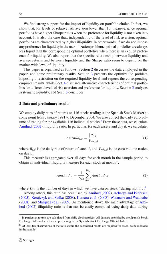
We employ daily rates of returns on 116 stocks trading in the Spanish Stock Market atsome point from January 1991 to December 2004. We also collect the daily euro vol-ume of trading for the available 116 individual stocks.7 From these data, we calculateAmihud (2002) illiquidity ratio. In particular, for each asset i and day d, we calculate,
Amihudi,d =∣∣Ri,d
∣∣
V oli,d(1)
where Ri,d is the daily rate of return of stock i , and V oli,d is the euro volume tradedon day d.
This measure is aggregated over all days for each month in the sample period toobtain an individual illiquidity measure for each stock at month t ,
Amihudi,t = 1
Di,t
Di,t∑
d=1
Amihudi,d (2)
where Di,t is the number of days in which we have data on stock i during month t .8
Among others, this ratio has been used by Amihud (2002), Acharya and Pedersen(2005), Korajczyk and Sadka (2008), Kamara et al. (2008), Watanabe and Watanabe(2008), and Márquez et al. (2009). As mentioned above, the main advantage of Ami-hud (2002) illiquidity ratio is that can be easily computed using daily data during
7 In particular, returns are calculated from daily closing prices. All data are provided by the Spanish StockExchange. All stocks in the sample belong to the Spanish Stock Exchange Official Index.8 At least ten observations of the ratio within the considered month are required for asset i to be includedin the sample.
123
SERIEs (2011) 2:53–74 57
long periods of time. Moreover, Hasbrouck (2009) shows that, at least for US data,Amihud (2002) ratio better approximates Kyle’s lambda relative to competing mea-sures of illiquidity.9
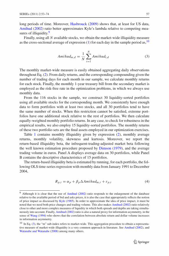
Finally, using all N available stocks, we obtain the market-wide illiquidity measureas the cross-sectional average of expression (1) for each day in the sample period as,10
Amihudm,d = 1
N
N∑
i=1
Amihudi,d (3)
The monthly market-wide measure is easily obtained aggregating daily observationsthroughout Eq. (2). From daily returns, and the corresponding compounding given thenumber of trading days for each month in our sample, we calculate monthly returnsfor each stock. Finally, the monthly 1-year treasury bill from the secondary market isemployed as the risk-free rate in the optimization problems, in which we always usemonthly data.
From the 116 stocks in the sample, we construct 30 liquidity-sorted portfoliosusing all available stocks for the corresponding month. We consistently have enoughdata to form portfolios with at least two stocks, and all 30 portfolios tend to havethe same number of stocks. When this restriction cannot be satisfied, extreme port-folios have one additional stock relative to the rest of portfolios. We then calculateequally-weighted monthly portfolio returns. In any case, to check for robustness in theempirical results, we also employ 15 liquidity-sorted portfolios. The monthly returnsof these two portfolio sets are the final assets employed in our optimization exercises.
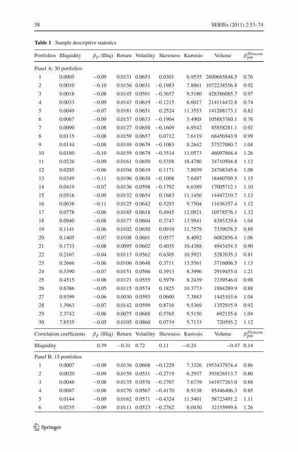
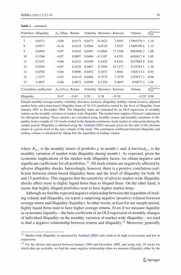
Table 1 contains monthly illiquidity given by expression (2), monthly averagereturns, monthly volatility, skewness and kurtosis. Moreover, we report thereturn-based illiquidity beta, the infrequent-trading-adjusted market beta followingthe well known estimation procedure proposed by Dimson (1979), and the averagetrading volume in euros. Panel A displays average data on 30 portfolios, while PanelB contains the descriptive characteristics of 15 portfolios.
The return-based illiquidity beta is estimated by running, for each portfolio, the fol-lowing OLS time-series regression with monthly data from January 1991 to December2004,
Rp,t = αp + βp�Amihudm,t + εp,t (4)
9 Although it is clear that the use of Amihud (2002) ratio responds to the enlargement of the databaserelative to the available period of bid and asks prices, it is also the case that appropriately reflects the notionof price impact as discussed by Kyle (1985). In order to approximate the idea of price impact, it must benoted that we need both price changes and trading volume. This also makes Amihud (2002) ratio relativelyclose to other and more complex measures of liquidity in which both spreads and depths are taking simulta-neously into account. Finally, Amihud (2002) ratio is also a natural proxy for information asymmetry, in thesense of Wang (1994) who shows that the correlation between absolute return and dollar volume increasesin information asymmetry.10 In Eq. (3), the “m” sub-index refers to market-wide. This aggregation procedure to obtain a representa-tive measure of market-wide illiquidity is a very common approach in literature. See Amihud (2002), andWatanabe and Watanabe (2008) among many others.
123
58 SERIEs (2011) 2:53–74
Table 1 Sample descriptive statistics
Portfolios Illiquidity βp (Illiq) Return Volatility Skewness Kurtosis Volume βDimsonpm
Panel A: 30 portfolios
1 0.0005 −0.09 0.0131 0.0653 0.0301 6.9535 2600665848.5 0.76
2 0.0010 −0.10 0.0156 0.0631 −0.1983 7.8861 1072238556.8 0.92
3 0.0018 −0.08 0.0145 0.0591 −0.3657 9.5180 428386085.7 0.97
4 0.0033 −0.09 0.0143 0.0619 −0.1215 6.6017 214114432.8 0.74
5 0.0049 −0.07 0.0181 0.0651 0.2524 11.3553 141288173.1 0.82
6 0.0067 −0.09 0.0157 0.0633 −0.1904 5.4905 105883760.1 0.76
7 0.0090 −0.08 0.0127 0.0658 −0.1609 6.9542 85858281.1 0.92
8 0.0115 −0.08 0.0159 0.0657 0.0712 7.6119 68456943.9 0.99
9 0.0144 −0.08 0.0149 0.0679 −0.1083 8.2642 57527080.7 1.04
10 0.0180 −0.10 0.0159 0.0679 −0.3514 11.0573 46097868.4 1.26
11 0.0226 −0.09 0.0161 0.0650 0.5358 18.4780 34710504.8 1.12
12 0.0285 −0.06 0.0104 0.0619 0.1171 7.8039 24768345.6 1.08
13 0.0349 −0.11 0.0196 0.0630 −0.1008 7.6487 18460709.5 1.15
14 0.0419 −0.07 0.0136 0.0598 −0.1792 6.6389 17005712.1 1.10
15 0.0516 −0.09 0.0132 0.0654 0.1683 11.1456 14447210.7 1.13
16 0.0638 −0.11 0.0125 0.0642 0.5293 9.7504 11636357.4 1.12
17 0.0778 −0.06 0.0185 0.0618 0.4945 12.0921 10578576.1 1.32
18 0.0940 −0.08 0.0177 0.0604 0.3747 13.9941 8385329.6 1.04
19 0.1141 −0.06 0.0102 0.0650 0.0910 11.7579 7339078.5 0.89
20 0.1405 −0.07 0.0108 0.0601 0.0577 8.4092 6082856.4 1.06
21 0.1733 −0.08 0.0095 0.0602 0.4035 10.4388 4943454.5 0.90
22 0.2167 −0.04 0.0113 0.0562 0.6305 10.5921 5287035.3 0.81
23 0.2666 −0.06 0.0106 0.0648 0.3711 13.5561 3716006.5 1.13
24 0.3390 −0.07 0.0151 0.0566 0.3913 8.3996 2919455.0 1.21
25 0.4515 −0.08 0.0121 0.0555 0.5979 8.2439 2339546.0 0.98
26 0.6386 −0.05 0.0115 0.0574 0.1825 10.3773 1884289.9 0.88
27 0.9399 −0.06 0.0030 0.0593 0.0600 7.3883 1445103.6 1.04
28 1.3963 −0.07 0.0142 0.0599 0.8716 9.5369 1352915.9 0.92
29 2.3742 −0.06 0.0075 0.0688 0.5765 9.5150 692155.6 1.04
30 7.8535 −0.05 0.0105 0.0860 0.0719 5.7133 720595.2 1.12
Correlation coefficients βp (Illiq) Return Volatility Skewness Kurtosis Volume βDimsonpm
Illiquidity 0.39 −0.31 0.72 0.11 −0.24 −0.47 0.14
Panel B: 15 portfolios
1 0.0007 −0.09 0.0136 0.0608 −0.1229 7.3326 1953437974.4 0.86
2 0.0020 −0.09 0.0159 0.0531 −0.2719 6.2937 393826513.7 0.80
3 0.0048 −0.08 0.0135 0.0576 −0.2707 7.6739 141977263.0 0.88
4 0.0087 −0.08 0.0176 0.0567 −0.4170 8.9138 85446406.3 0.85
5 0.0144 −0.09 0.0162 0.0571 −0.4324 11.5401 58723491.2 1.11
6 0.0235 −0.09 0.0111 0.0523 −0.2762 8.0430 32155999.6 1.26
123
SERIEs (2011) 2:53–74 59
Table 1 continued
Portfolios Illiquidity βp (Illiq) Return Volatility Skewness Kurtosis Volume βDimsonpm
7 0.0371 −0.08 0.0172 0.0473 −0.3623 7.0397 17965578.3 1.10
8 0.0577 −0.10 0.0135 0.0504 0.0720 7.9357 13409789.6 1.19
9 0.0894 −0.07 0.0162 0.0483 −0.0968 17.3188 8883860.2 1.08
10 0.1386 −0.07 0.0097 0.0486 −0.1107 8.4791 6436817.4 1.05
11 0.2247 −0.06 0.0122 0.0450 0.2429 8.8161 4527085.8 0.81
12 0.3656 −0.07 0.0129 0.0467 0.2549 10.1277 3118782.1 1.20
13 0.6704 −0.06 0.0096 0.0452 0.1833 7.8661 1768115.4 0.95
14 1.3277 −0.07 0.0110 0.0486 0.3575 7.7270 1355517.3 0.98
15 5.4855 −0.06 0.0072 0.0598 0.1220 5.8697 670877.3 1.06
Correlation coefficients βp(I lliq) Return Volatility Skewness Kurtosis Volume βDimsonpm
Illiquidity 0.47 −0.63 0.29 0.38 −0.30 −0.55 0.08
Sample monthly average returns, volatility, skewness, kurtosis, illiquidity, trading volume in euros, adjustedmarket betas and return-based illiquidity betas of 30 (15) portfolios sorted by the level of illiquidity fromJanuary 1991 to December 2004. The illiquidity betas are estimated by an OLS regression of monthlyreturns on the monthly variation of market-wide illiquidity. The market beta employs Dimson’s adjustmentfor infrequent trading. These statistics are calculated using monthly returns and monthly variations of illi-quidity from a sample of 116 stocks traded in the Spanish continuous stock market at some point during thesample period. Illiquidity is obtained using the Amihud (2002) measure given by the ratio of the absolutereturn of a given stock to the euro volume of the stock. The correlation coefficient between illiquidity andtrading volume is calculated by taking first the logarithm of trading volume
where Rp,t is the monthly return of portfolio p in month t , and �Amihudm,t is themonthly variation of market-wide illiquidity during month t . As expected, given theeconomic implications of the market-wide illiquidity factor, we obtain negative andsignificant coefficients for all portfolios.11 All stock returns are negatively affected byadverse illiquidity shocks. Interestingly, however, there is a positive correlation coef-ficient between return-based illiquidity betas and the level of illiquidity for both 30and 15 portfolios. This suggests that the sensitivity of adverse market-wide illiquidityshocks affect more to highly liquid firms than to illiquid firms. On the other hand, itseems that highly illiquid portfolios tend to have higher market betas.
Although we find the expected negative relationship between (the logarithm of) trad-ing volume and illiquidity, we report a surprising negative (positive) relation betweenaverage return and illiquidity (liquidity). In other words, at least for our sample period,highly liquid firms tend to have higher average returns. Even if we measure liquidityas systematic liquidity—the beta coefficient of an OLS regression of monthly changesof individual illiquidity on the monthly variation of market-wide illiquidity—we tendto find a negative relationship between returns and illiquidity.12 Moreover, generally
11 Market-wide illiquidity as measured by Amihud (2002) ratio tends to be high in recessions and low inexpansions.12 For the shorter time-period between January 1996 and December 2000, and using only 29 stocks forwhich data are available, we find the same negative relationship when we measure illiquidity either by the
123
60 SERIEs (2011) 2:53–74
speaking, we report negative skewness for highly liquid firms, while positive skew-ness characterizes highly illiquid stocks.13 Finally, as expected, there is a positivecorrelation between illiquidity and volatility.
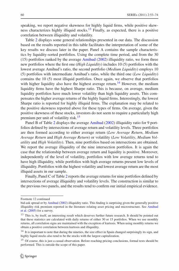
Table 2 displays some general relationships presented in our data. The discussionbased on the results reported in this table facilitates the interpretation of some of thekey results we discuss later in the paper. Panel A contains the sample characteris-tics by liquidity-sorted portfolios. Using the complete time period, and from the 30(15) portfolios ranked by the average Amihud (2002) illiquidity ratio, we form threenew portfolios where the first one (High Liquidity) includes 10 (5) portfolios with thelowest average Amihud’s ratio, the second portfolio (Medium Liquidity) employs 10(5) portfolios with intermediate Amihud’s ratio, while the third one (Low Liquidity)contains the 10 (5) most illiquid portfolios. Once again, we observe that portfolioswith higher liquidity also have the highest average return.14 However, the mediumliquidity firms have the highest Sharpe ratio. This is because, on average, mediumliquidity portfolios have much lower volatility than high liquidity assets. This com-pensates the higher average returns of the highly liquid firms. Interestingly, the lowestSharpe ratio is reported for highly illiquid firms. The explanation may be related tothe positive skewness reported above for these types of firms. On average, given thepositive skewness of these stocks, investors do not seem to require a particularly highpremium per unit of volatility risk.15
Panel B of Table 2 displays the average Amihud (2002) illiquidity ratio for 9 port-folios defined by intersections of average return and volatility levels. Three portfoliosare then formed according to either average return (Low Average Return, MediumAverage Return and High Average Return) or volatility (Low Volatility, Medium Vol-atility and High Volatility). Then, nine portfolios based on intersections are obtained.We report the average illiquidity of the nine intersection portfolios. It is again thecase that the relationship between average return and liquidity is positive. Moreover,independently of the level of volatility, portfolios with low average returns tend tohave high illiquidity, while portfolios with high average returns present low levels ofilliquidity. Portfolios with the highest volatility and lowest average return are the mostilliquid assets in our sample.
Finally, Panel C of Table 2 reports the average returns for nine portfolios defined byintersections of average illiquidity and volatility levels. The construction is similar tothe previous two panels, and the results tend to confirm our initial empirical evidence.
Footnote 12 continuedbid-ask spread or by Amihud (2002) illiquidity ratio. This finding is surprising given the generally positiveilliquidity risk premium reported in the literature relating asset pricing and microstructure. See Amihudet al. (2005) for a survey.13 This is, by itself, an interesting result which deserves further future research. It should be pointed outthat these statistics are calculated with daily returns of either 30 or 15 portfolios. When we use monthlyreturns, all correlation signs are maintained with the exception of kurtosis. When using monthly returns weobtain a positive correlation between kurtosis and illiquidity.14 It is important to note that during the nineties, the size effect in Spain changed surprisingly its sign, andhighly liquid stocks also tend to be the stocks with the largest capitalization.15 Of course, this is just a casual observation. Before reaching pricing conclusions, formal tests should beperformed. This is outside the scope of this paper.
123
SERIEs (2011) 2:53–74 61
Table 2 Liquidity, average returns and volatility
Average return Volatility of returns Sharpe ratio Illiquidity Amihud ratio
Panel A
30 Portfolios
High liquidity 0.0151 0.0487 0.2050 0.0071
Medium liquidity 0.0143 0.0382 0.2398 0.0670
Low liquidity 0.0105 0.0315 0.1721 1.4650
15 Portfolios
High liquidity 0.0154 0.0491 0.2089 0.0061
Medium liquidity 0.0135 0.0381 0.2219 0.0693
Low liquidity 0.0106 0.0315 0.1737 1.6148
Illiquidity Amihud ratio Low volatility Medium volatility High volatility
Panel B
30 Portfolios
Low average return 0.4218 0.1475 3.4473
Medium average return 0.4729 0.0335 0.0189
High average return 0.3390 0.0395 0.0115
15 Portfolios
Low average return 0.6704 0.4966 5.4855
Medium average return 0.2952 0.0577 0.0027
High average return 0.0632 0.0020 0.0115
Portfolio average return Low volatility Medium volatility High volatility
Panel C30 Portfolios
High liquidity 0.0145 0.0152 0.0151
Medium liquidity 0.0122 0.0158 0.0117
Low liquidity 0.0110 0.0106 0.0090
15 Portfolios
High liquidity NAa 0.0159 0.0152
Medium liquidity 0.0167 0.0114 NAa
Low liquidity 0.0116 0.0110 0.0072
Panel A: sample characteristics by liquidity-sorted portfolios. Using the complete time period from January 1991 to Decem-ber 2004, all 116 stocks traded at some point during the sample period are ranked by the Amihud (2002) average illiquidityratio. Three portfolios are then formed where the first one (High Liquidity) includes ten portfolios (5 portfolios) with thelowest illiquidity ratio, the second portfolio (Medium Liquidity) employs ten (5) portfolios with intermediate ratio, whilethe third one (Low Liquidity) contains the ten (5) most illiquid portfolios. Panel B: It contains the Amihud (2002) averageilliquidity ratio for 9 portfolios based on intersections between 30 (15) portfolios sorted (separately) by average returnand volatility, using the complete time period from January 1991 to December 2004. Three portfolios are then formedaccording to either average return (Low Average Return, Medium Average Return and High Average Return) or volatility(Low Volatility, Medium Volatility and High Volatility). We finally calculate Amihud (2002) average illiquidity ratio ofthe nine intersection portfolios. Panel C: It reports average returns for 9 portfolios based on intersections between 30 (15)portfolios sorted (separately) by the Amihud (2002) average illiquidity ratio and volatility, using the complete time periodfrom January 1991 to December 2004. Three portfolios are then formed according to either average illiquidity ratio (HighLiquidity, Medium Liquidity and Low Liquidity) or volatility (Low Volatility, Medium Volatility and High Volatility). Then,we calculate the average returns of the nine intersection portfoliosa Portfolio is empty
123
62 SERIEs (2011) 2:53–74
Independently of the level of volatility, portfolios with low liquidity tend to obtain lowaverage returns.
3 The mean-variance liquidity-constrained frontier
In this section, we obtain the minimum variance frontier by imposing not only the tra-ditional constraint on average return, but also an additional constraint on a minimumrequired level of liquidity.
The mean-variance liquidity constrained frontier is obtained by solving the follow-ing optimization problem:
minω
1
2ω′V ω
subject to
⎧
⎪⎪⎨
⎪⎪⎩
ω′μ = μp
ω′ Amihud = Amihudp
ω′1N = 1ω ≥ 0
(5)
where V is the N ×N variance-covariance matrix of monthly portfolio returns, μ is theN -vector of monthly mean portfolio returns, Amihud is the N -vector of monthly portfo-lio illiquidity, μp and Amihudp are the required levels of average return and illiquidityon the minimum variance liquidity constrained portfolio, and ω are the non-negativeweights of each portfolio on the minimum variance liquidity constrained portfolio.We solve this problem for N = 30 and N = 15 illiquidity-sorted portfolios.16
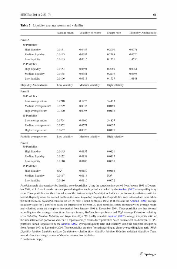
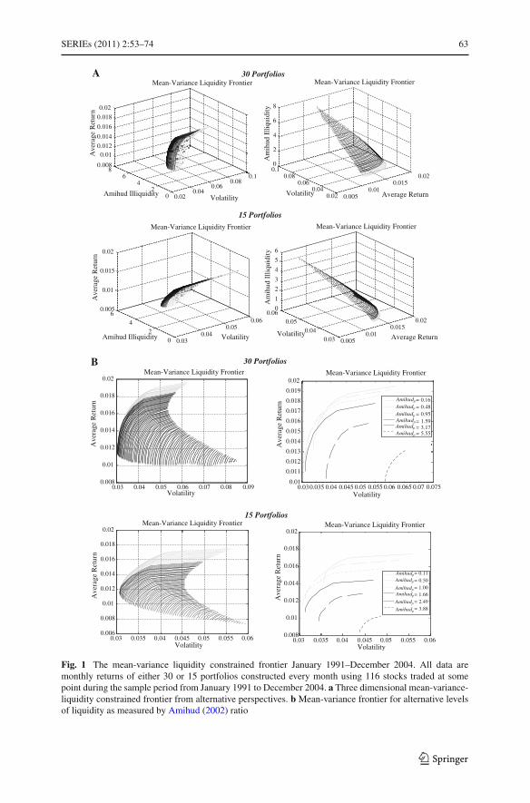
Panel A of Fig. 1 displays the three-dimensional mean-variance liquidity con-strained frontier, while Panel B contains the mean-variance frontier for alternativelevels of liquidity. Both figures contain the results for 30 and 15 portfolios, and PanelA shows the three-dimensional frontiers from two different perspectives. For eachportfolio illiquidity level between 5 × 10⁻⁴ and 7.85, for N = 30, and between7 × 10−4 and 5.49 for N = 15, we obtain two different frontiers depending uponthe behaviour of returns, volatility and liquidity. For high levels of liquidity, given byAmihud (2002) illiquidity ratio between 5 × 10⁻⁴ and 0.95, for N = 30, and between7 × 10−4 and 1, for N = 15, the frontier in terms of average return depends not onlyon illiquidity but also on volatility. For low levels of volatility, the frontier moves asexpected. This means that higher illiquidity is associated with higher average returns.On the other hand, for high levels of volatility, higher illiquidity is accompanied withlower average returns. This also occurs for high levels of illiquidity in which Amihud(2002) ratio is between 0.95 and 7.85 for N = 30, and between 1 and 5.49 for N = 15.Once again, in this case, the frontier moves contrary to our expectation. These two
16 We understand that the liquidity restriction is assumed to be linear, to affect all stocks, and to be binding.There may be alternative specifications to the problem given by Eq. (5) above. For example, as pointed outby one of the referees, it may be the case that investors were only interested in guarantying a minimumliquidity level for some of the stocks. In fact, Sect. 4 below recognizes explicitly the preference for liquidityin the objective function.
123
SERIEs (2011) 2:53–74 63
30 Portfolios
0.020.04
0.060.08
0.1
02
46
80.008
0.010.012
0.014
0.016
0.018
0.02
Volatility
Mean-Variance Liquidity Frontier
Amihud Illiquidity
Ave
rage
Retur
n
0.0050.01
0.0150.02
0.020.04
0.060.08
0.10
2
4
6
8
Am
ihud
Ill
iqui
dity
Mean-Variance Liquidity Frontier
Average ReturnVolatility
15 Portfolios
0.030.04
0.050.06
02
46
0.005
0.01
0.015
0.02
Volatility
Mean-Variance Liquidity Frontier
Amihud Illiquidity
Ave
rage
Retur
n
0.0050.01
0.0150.02
0.030.04
0.050.06
0
1
2
3
4
5
6
Am
ihud
Ill
iqui
dity
Mean-Variance Liquidity Frontier
Average ReturnVolatility
30 Portfolios
0.03 0.04 0.05 0.06 0.07 0.08 0.090.008
0.01
0.012
0.014
0.016
0.018
0.02Mean-Variance Liquidity Frontier
Volatility
Ave
rage
Retur
n
0.030.035 0.04 0.045 0.05 0.055 0.06 0.065 0.07 0.0750.01
0.011
0.012
0.013
0.014
0.015
0.016
0.017
0.018
0.019
0.02Mean-Variance Liquidity Frontier
Volatility
Ave
rage
Retur
n
15 Portfolios
0.03 0.035 0.04 0.045 0.05 0.055 0.060.006
0.008
0.01
0.012
0.014
0.016
0.018
0.02Mean-Variance Liquidity Frontier
Volatility
Ave
rage
Retur
n
0.03 0.035 0.04 0.045 0.05 0.055 0.060.008
0.01
0.012
0.014
0.016
0.018
0.02Mean-Variance Liquidity Frontier
Volatility
Ave
rage
Retur
n
= 0.11= 0.50= 1.00= 1.66= 2.49= 3.88
A
B
= 0.16= 0.48= 0.95= 1.59= 3.17= 5.55
Amihudp
Amihudp
Amihudp
AmihudpAmihudp
Amihudp
Amihudp
Amihudp
Amihudp
Amihudp
Amihudp
Amihudp
Fig. 1 The mean-variance liquidity constrained frontier January 1991–December 2004. All data aremonthly returns of either 30 or 15 portfolios constructed every month using 116 stocks traded at somepoint during the sample period from January 1991 to December 2004. a Three dimensional mean-variance-liquidity constrained frontier from alternative perspectives. b Mean-variance frontier for alternative levelsof liquidity as measured by Amihud (2002) ratio
123
64 SERIEs (2011) 2:53–74
different types of behaviour of the three-dimensional frontier are represented by a darkarea in the first case, and a light zone in the second case.
These results suggest that it is important to simultaneously consider the interplaybetween average returns, volatility and illiquidity. This is an interesting result whichalready implies that liquidity as a characteristic plays a role on determining optimalportfolios.
To be more precise, we calculate the tangency portfolio for each efficient frontiergiven a level of liquidity. In particular, we maximize the Sharpe ratio as follows,
maxω
μp − r f
σp
subject to
⎧
⎪⎪⎪⎪⎨
⎪⎪⎪⎪⎩
ω′μ + (
1 − ω′1N)
r f = μp√ω′V ω = σp
ω′ Amihud = Amihudp
ω′1N = 1ω ≥ 0
(6)
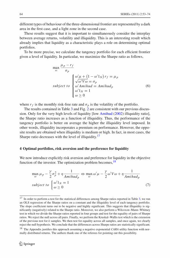
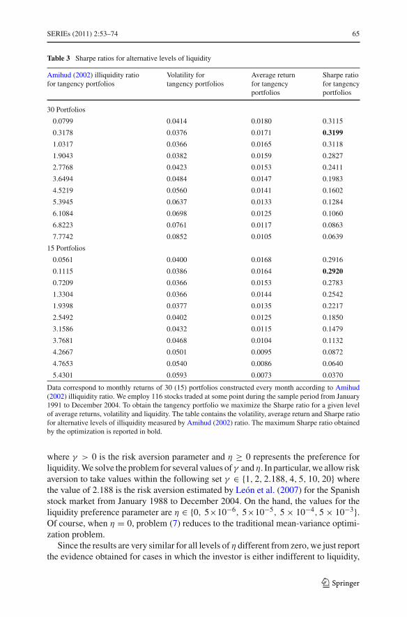
where r f is the monthly risk-free rate and σp is the volatility of the portfolio.The results contained in Table 3 and Fig. 2 are consistent with our previous discus-
sion. Only for the very high levels of liquidity [low Amihud (2002) illiquidity ratio],the Sharpe ratio increases as a function of illiquidity. Thus, the performance of thetangency portfolio is better on average the higher the illiquidity level imposed. Inother words, illiquidity incorporates a premium on performance. However, the oppo-site results are obtained when illiquidity is medium or high. In fact, in most cases, theSharpe ratio decreases with the level of illiquidity.17
4 Optimal portfolios, risk aversion and the preference for liquidity
We now introduce explicitly risk aversion and preference for liquidity in the objectivefunction of the investor. The optimization problem becomes,18
maxω
μp − γ
2σ 2
p + η1
Amihudp⇔ max
ωω′μ − γ
2ω′V ω + η
1
Amihudp
subject to
{
ω′1N = 1ω ≥ 0
(7)
17 In order to perform a test for the statistical differences among Sharpe ratios reported in Table 3, we runan OLS regression of the Sharpe ratios on a constant and the illiquidity level of each tangency portfolio.The slope coefficient turns out to be negative and highly significant. This suggests that illiquidity is sig-nificantly (negatively) related to the Sharpe ratio. Moreover, we also perform a Wilcoxon–Mann–Whitneytest in which we divide the Sharpe ratios reported in four groups and test for the equality of pairs of Sharperatios. We reject the null across all pairs. Finally, we perform the Kruskal–Wallis test which is the extensionof the previous test for k samples. We then test for equality across all samples, and once again, we clearlyreject the null hypothesis. We conclude that the differences across Sharpe ratios are statistically significant.18 The Appendix justifies this approach assuming a negative exponential CARA utility function with nor-mally distributed returns. The authors thank one of the referees for pointing out this possibility.
123
SERIEs (2011) 2:53–74 65
Table 3 Sharpe ratios for alternative levels of liquidity
Amihud (2002) illiquidity ratio Volatility for Average return Sharpe ratiofor tangency portfolios tangency portfolios for tangency for tangency
portfolios portfolios
30 Portfolios
0.0799 0.0414 0.0180 0.3115
0.3178 0.0376 0.0171 0.3199
1.0317 0.0366 0.0165 0.3118
1.9043 0.0382 0.0159 0.2827
2.7768 0.0423 0.0153 0.2411
3.6494 0.0484 0.0147 0.1983
4.5219 0.0560 0.0141 0.1602
5.3945 0.0637 0.0133 0.1284
6.1084 0.0698 0.0125 0.1060
6.8223 0.0761 0.0117 0.0863
7.7742 0.0852 0.0105 0.0639
15 Portfolios
0.0561 0.0400 0.0168 0.2916
0.1115 0.0386 0.0164 0.2920
0.7209 0.0366 0.0153 0.2783
1.3304 0.0366 0.0144 0.2542
1.9398 0.0377 0.0135 0.2217
2.5492 0.0402 0.0125 0.1850
3.1586 0.0432 0.0115 0.1479
3.7681 0.0468 0.0104 0.1132
4.2667 0.0501 0.0095 0.0872
4.7653 0.0540 0.0086 0.0640
5.4301 0.0593 0.0073 0.0370
Data correspond to monthly returns of 30 (15) portfolios constructed every month according to Amihud(2002) illiquidity ratio. We employ 116 stocks traded at some point during the sample period from January1991 to December 2004. To obtain the tangency portfolio we maximize the Sharpe ratio for a given levelof average returns, volatility and liquidity. The table contains the volatility, average return and Sharpe ratiofor alternative levels of illiquidity measured by Amihud (2002) ratio. The maximum Sharpe ratio obtainedby the optimization is reported in bold.
where γ > 0 is the risk aversion parameter and η ≥ 0 represents the preference forliquidity. We solve the problem for several values of γ and η. In particular, we allow riskaversion to take values within the following set γ ∈ {1, 2, 2.188, 4, 5, 10, 20} wherethe value of 2.188 is the risk aversion estimated by León et al. (2007) for the Spanishstock market from January 1988 to December 2004. On the hand, the values for theliquidity preference parameter are η ∈ {0, 5×10⁻⁶, 5×10⁻⁵, 5 × 10⁻⁴, 5 × 10⁻³}.Of course, when η = 0, problem (7) reduces to the traditional mean-variance optimi-zation problem.
Since the results are very similar for all levels of η different from zero, we just reportthe evidence obtained for cases in which the investor is either indifferent to liquidity,
123
66 SERIEs (2011) 2:53–74
0 1 2 3 4 5 6 7 80.05
0.1
0.15
0.2
0.25
0.3
0.35
0.4
X: 0.3178Y: 0.3199
Sharpe Ratio for Tangency Portfolios30 Portfolios 15 Portfolios
Amihud Illiquidity
0 1 2 3 4 5 60
0.05
0.1
0.15
0.2
0.25
0.3
0.35Sharpe Ratio for Tangency Portfolios
Amihud Illiquidity
X: 0.1115Y: 0.292
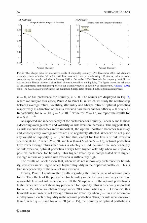
Fig. 2 The Sharpe ratio for alternative levels of illiquidity January 1991–December 2004. All data aremonthly returns of either 30 or 15 portfolios constructed every month using 116 stocks traded at somepoint during the sample period from January 1991 to December 2004. To obtain the tangency portfolio wemaximize the Sharpe ratio for a given level of return, volatility, and liquidity. The figure shows the behaviorof the Sharpe ratio of the tangency portfolio for alternative levels of liquidity as measured by Amihud (2002)ratio. The black square point shows the maximum Sharpe ratio obtained in the optimization process
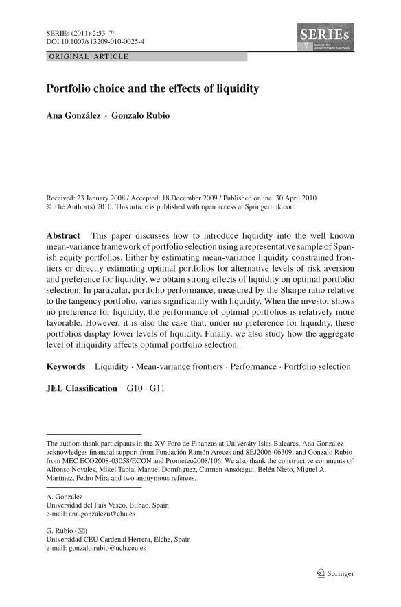
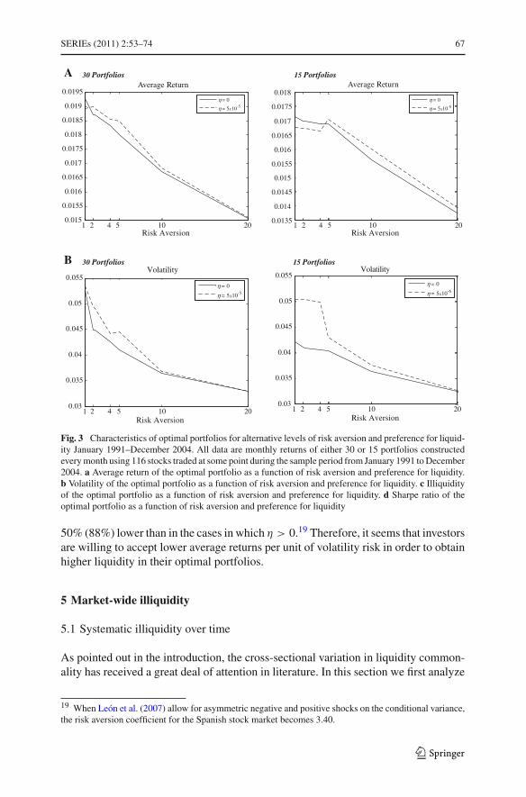
η = 0, or has preference for liquidity, η > 0. The results are displayed in Fig. 3,where we analyze four cases, Panel A to Panel D, in which we study the relationshipbetween average return, volatility, illiquidity and Sharpe ratio of optimal portfoliosrespectively as a function of the risk aversion parameter and for either η = 0 or η > 0.In particular, for N = 30, η = 5 × 10⁻⁵ while for N = 15, we report the results forη = 5 × 10⁻⁶.
As expected and independently of the preference for liquidity, Panels A and B showa declining average return and volatility as risk aversion increases. This suggests that,as risk aversion becomes more important, the optimal portfolio becomes less riskyand, consequently, average returns are also negatively affected. When we do not placeany weight on liquidity, η = 0, we find that, except for low levels of risk aversioncoefficients (<1.5 when N = 30, and less than 4.5 when N = 15), optimal portfolioshave lower average returns than cases in which η > 0. At the same time, independentlyof risk aversion, optimal portfolios always have higher volatility when we impose apositive preference for liquidity. This higher volatility is compensated with higheraverage returns only when risk aversion is sufficiently high.
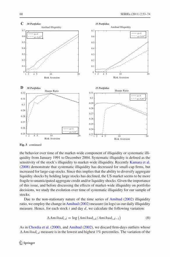
The results of Panel C show that, when we do not impose any preference for liquid-ity, investors are willing to accept higher illiquidity in their optimal portfolios. This istrue independently of the level of risk aversion.
Finally, Panel D contains the results regarding the Sharpe ratio of optimal port-folios. The effects of the preference for liquidity on performance are very clear. Forreasonable levels of risk aversion, γ < 10, the Sharpe ratio of the optimal portfolios ishigher when we do not show any preference for liquidity. This is especially importantfor N = 15, where we obtain Sharpe ratios 20% lower when η > 0. Of course, thisfavorable result in terms of average returns and volatility when η = 0 is also accompa-nied by lower levels of liquidity in the optimal portfolios. Thus, for risk aversion lowerthan 5, when η = 0 and for N = 30 (N = 15), the liquidity of optimal portfolios is
123
SERIEs (2011) 2:53–74 67
1 2 4 5 10 20 0.015
0.0155
0.016
0.0165
0.017
0.0175
0.018
0.0185
0.019
0.0195
30 Portfolios
30 Portfolios 15 Portfolios
15 Portfolios Average Return
Risk Aversion
η = 0
η = 5x10⁻⁵
1 2 4 5 10 200.0135
0.014
0.0145
0.015
0.0155
0.016
0.0165
0.017
0.0175
0.018Average Return
Risk Aversion
η = 0
η = 5x10⁻⁶
1 2 4 5 10 200.03
0.035
0.04
0.045
0.05
0.055Volatility
Risk Aversion1 2 4 5 10 20
0.03
0.035
0.04
0.045
0.05
0.055Volatility
Risk Aversion
η = 0
η = 5x10⁻⁵
η = 0
η = 5x10⁻⁶
A
B
Fig. 3 Characteristics of optimal portfolios for alternative levels of risk aversion and preference for liquid-ity January 1991–December 2004. All data are monthly returns of either 30 or 15 portfolios constructedevery month using 116 stocks traded at some point during the sample period from January 1991 to December2004. a Average return of the optimal portfolio as a function of risk aversion and preference for liquidity.b Volatility of the optimal portfolio as a function of risk aversion and preference for liquidity. c Illiquidityof the optimal portfolio as a function of risk aversion and preference for liquidity. d Sharpe ratio of theoptimal portfolio as a function of risk aversion and preference for liquidity
50% (88%) lower than in the cases in which η > 0.19 Therefore, it seems that investorsare willing to accept lower average returns per unit of volatility risk in order to obtainhigher liquidity in their optimal portfolios.
5 Market-wide illiquidity
5.1 Systematic illiquidity over time
As pointed out in the introduction, the cross-sectional variation in liquidity common-ality has received a great deal of attention in literature. In this section we first analyze
19 When León et al. (2007) allow for asymmetric negative and positive shocks on the conditional variance,the risk aversion coefficient for the Spanish stock market becomes 3.40.
123
68 SERIEs (2011) 2:53–74
1 2 4 5 10 200
0.1
0.2
0.3
0.4
0.5
0.6
0.7
30 Portfolios
30 Portfolios
15 Portfolios
15 Portfolios
Amihud Illiquidity
Risk Aversion
η = 0
η = 5x10⁻⁵
η = 0
η = 5x10⁻⁵
η = 0
η = 5x10⁻⁶
η = 0
η = 5x10⁻⁶
1 2 4 5 10 200
0.1
0.2
0.3
0.4
0.5
0.6
0.7
Amihud Illiquidity
Risk Aversion
1 2 4 5 10 200.25
0.26
0.27
0.28
0.29
0.3
0.31
0.32Sharpe Ratio
Risk Aversion1 2 4 5 10 20
0.23
0.24
0.25
0.26
0.27
0.28
0.29
0.3
0.31Sharpe Ratio
Risk Aversion
C
D
Fig. 3 continued
the behavior over time of the market-wide component of illiquidity or systematic illi-quidity from January 1991 to December 2004. Systematic illiquidity is defined as thesensitivity of the stock’s illiquidity to market-wide illiquidity. Recently Kamara et al.(2008) demonstrate that systematic illiquidity has decreased for small-cap firms, butincreased for large-cap stocks. Since this implies that the ability to diversify aggregateliquidity shocks by holding large stocks has declined, the US market seems to be morefragile to unanticipated aggregate credit and/or liquidity shocks. Given the importanceof this issue, and before discussing the effects of market-wide illiquidity on portfoliodecisions, we study the evolution over time of systematic illiquidity for our sample ofstocks.
Due to the non-stationary nature of the time series of Amihud (2002) illiquidityratio, we employ the change in Amihud (2002) measure (in logs) as our daily illiquiditymeasure. Hence, for each stock i and day d, we calculate the following variation:
�Amihudi,d = log(
Amihudi,d/Amihudi,d−1)
(8)
As in Chordia et al. (2000), and Amihud (2002), we discard firm-days outliers whose�Amihudi,d measure is in the lowest and highest 1% percentiles. The variation of the
123
SERIEs (2011) 2:53–74 69
Dec-1997 Dec-2000 Dec-20040
1
2
3
4
5
6
7
8Aggregate Illiquidity: Amihudm ,d
1991 1994 1997 2000 2003 2005-3
-2
-1
0
1
2
3Market Illiquidity Variation: ΔAmihudm ,d
1991 1993 1997 2000 20040.25
0.3
0.35
0.4
0.45
0.5Volatility of ΔAmihudm ,d
a
b1 b2
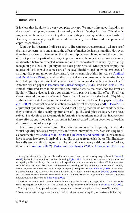
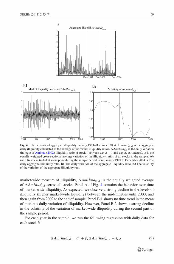
Fig. 4 The behavior of aggregate illiquidity January 1991–December 2004. Amihudm,d is the aggregatedaily illiquidity calculated as the average of individual illiquidity ratios. �Amihudi,d is the daily variation(in logs) of Amihud (2002) illiquidity ratio of stock i between day d − 1 and day d. �Amihudm,d is theequally weighted cross-sectional average variation of the illiquidity ratios of all stocks in the sample. Weuse 116 stocks traded at some point during the sample period from January 1991 to December 2004. a Thedaily aggregate illiquidity ratio. b1 The daily variation of the aggregate illiquidity ratio. b2 The volatilityof the variation of the aggregate illiquidity ratio
market-wide measure of illiquidity, �Amihudm,d , is the equally weighted averageof �Amihudi,d across all stocks. Panel A of Fig. 4 contains the behavior over timeof market-wide illiquidity. As expected, we observe a strong decline in the levels ofilliquidity (higher market-wide liquidity) between the mid-nineties until 2000, andthen again from 2002 to the end of sample. Panel B.1 shows no time trend in the meanof market’s daily variation of illiquidity. However, Panel B.2 shows a strong declinein the volatility of the variation of market-wide illiquidity during the second part ofthe sample period.
For each year in the sample, we run the following regression with daily data foreach stock i :
�Amihudi,d = αi + βi�Amihudm,d + εi,d (9)
123
70 SERIEs (2011) 2:53–74
1991 1994 1997 2000 2003−0.5
0
0.5
1
1.5Liquidity Beta for Small and Large Firms
1991 1994 1997 2000 2003−0.2
−0.1
0
0.1
0.2
0.3
0.4
0.5Difference in Liquidity Beta between Large and Small Firms
SmallLarge
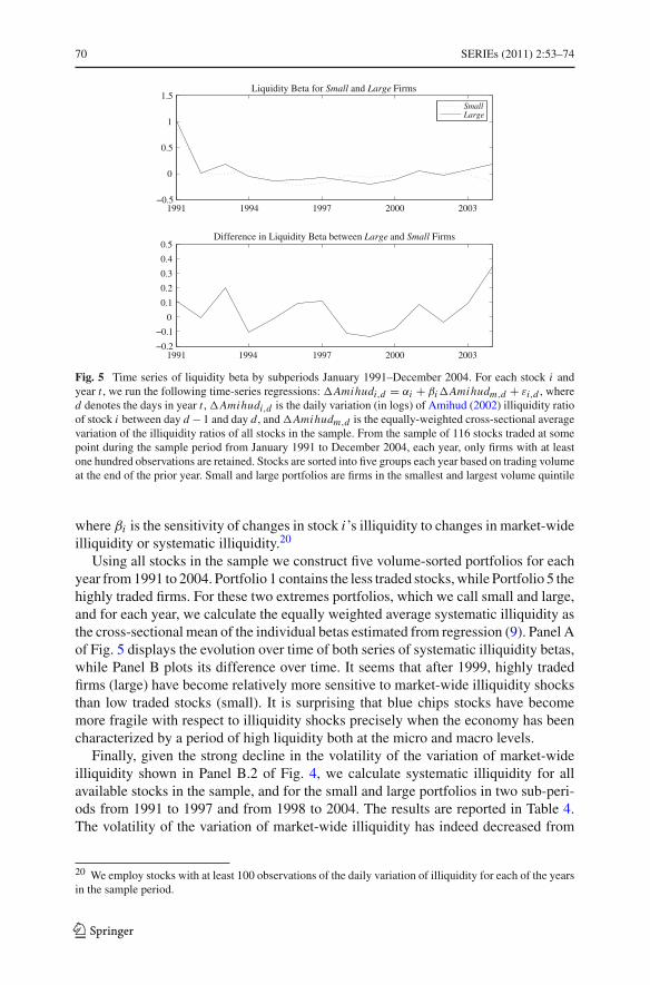
Fig. 5 Time series of liquidity beta by subperiods January 1991–December 2004. For each stock i andyear t , we run the following time-series regressions: �Amihudi,d = αi + βi �Amihudm,d + εi,d , whered denotes the days in year t , �Amihudi,d is the daily variation (in logs) of Amihud (2002) illiquidity ratioof stock i between day d − 1 and day d, and �Amihudm,d is the equally-weighted cross-sectional averagevariation of the illiquidity ratios of all stocks in the sample. From the sample of 116 stocks traded at somepoint during the sample period from January 1991 to December 2004, each year, only firms with at leastone hundred observations are retained. Stocks are sorted into five groups each year based on trading volumeat the end of the prior year. Small and large portfolios are firms in the smallest and largest volume quintile
where βi is the sensitivity of changes in stock i’s illiquidity to changes in market-wideilliquidity or systematic illiquidity.20
Using all stocks in the sample we construct five volume-sorted portfolios for eachyear from 1991 to 2004. Portfolio 1 contains the less traded stocks, while Portfolio 5 thehighly traded firms. For these two extremes portfolios, which we call small and large,and for each year, we calculate the equally weighted average systematic illiquidity asthe cross-sectional mean of the individual betas estimated from regression (9). Panel Aof Fig. 5 displays the evolution over time of both series of systematic illiquidity betas,while Panel B plots its difference over time. It seems that after 1999, highly tradedfirms (large) have become relatively more sensitive to market-wide illiquidity shocksthan low traded stocks (small). It is surprising that blue chips stocks have becomemore fragile with respect to illiquidity shocks precisely when the economy has beencharacterized by a period of high liquidity both at the micro and macro levels.
Finally, given the strong decline in the volatility of the variation of market-wideilliquidity shown in Panel B.2 of Fig. 4, we calculate systematic illiquidity for allavailable stocks in the sample, and for the small and large portfolios in two sub-peri-ods from 1991 to 1997 and from 1998 to 2004. The results are reported in Table 4.The volatility of the variation of market-wide illiquidity has indeed decreased from
20 We employ stocks with at least 100 observations of the daily variation of illiquidity for each of the yearsin the sample period.
123
SERIEs (2011) 2:53–74 71
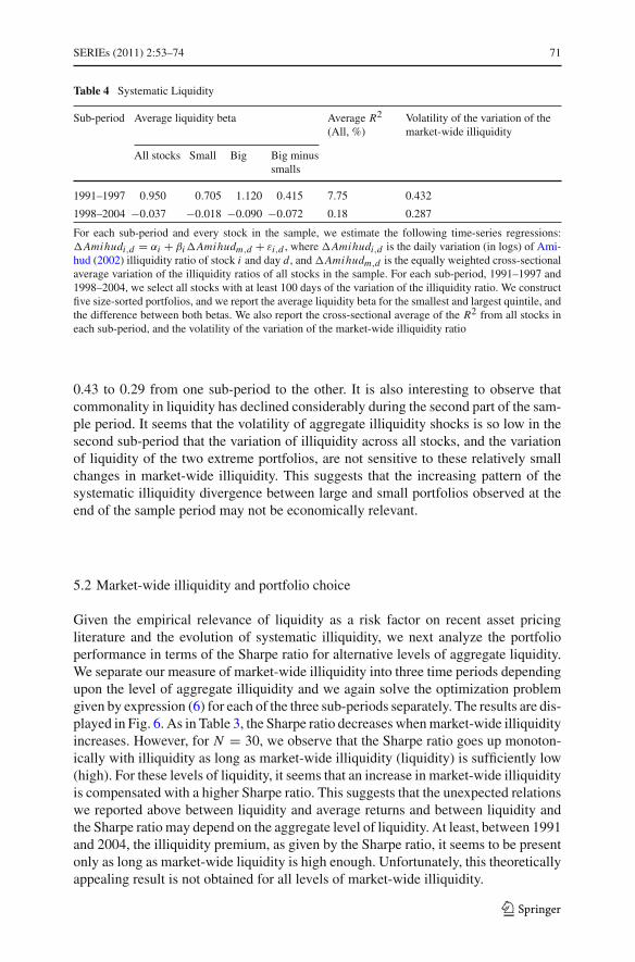
Table 4 Systematic Liquidity
Sub-period Average liquidity beta Average R2
(All, %)Volatility of the variation of themarket-wide illiquidity
All stocks Small Big Big minussmalls
1991–1997 0.950 0.705 1.120 0.415 7.75 0.432
1998–2004 −0.037 −0.018 −0.090 −0.072 0.18 0.287
For each sub-period and every stock in the sample, we estimate the following time-series regressions:�Amihudi,d = αi + βi �Amihudm,d + εi,d , where �Amihudi,d is the daily variation (in logs) of Ami-hud (2002) illiquidity ratio of stock i and day d, and �Amihudm,d is the equally weighted cross-sectionalaverage variation of the illiquidity ratios of all stocks in the sample. For each sub-period, 1991–1997 and1998–2004, we select all stocks with at least 100 days of the variation of the illiquidity ratio. We constructfive size-sorted portfolios, and we report the average liquidity beta for the smallest and largest quintile, andthe difference between both betas. We also report the cross-sectional average of the R2 from all stocks ineach sub-period, and the volatility of the variation of the market-wide illiquidity ratio
0.43 to 0.29 from one sub-period to the other. It is also interesting to observe thatcommonality in liquidity has declined considerably during the second part of the sam-ple period. It seems that the volatility of aggregate illiquidity shocks is so low in thesecond sub-period that the variation of illiquidity across all stocks, and the variationof liquidity of the two extreme portfolios, are not sensitive to these relatively smallchanges in market-wide illiquidity. This suggests that the increasing pattern of thesystematic illiquidity divergence between large and small portfolios observed at theend of the sample period may not be economically relevant.
5.2 Market-wide illiquidity and portfolio choice
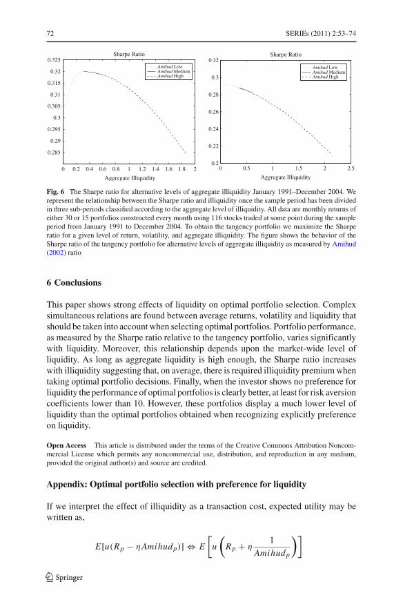
Given the empirical relevance of liquidity as a risk factor on recent asset pricingliterature and the evolution of systematic illiquidity, we next analyze the portfolioperformance in terms of the Sharpe ratio for alternative levels of aggregate liquidity.We separate our measure of market-wide illiquidity into three time periods dependingupon the level of aggregate illiquidity and we again solve the optimization problemgiven by expression (6) for each of the three sub-periods separately. The results are dis-played in Fig. 6. As in Table 3, the Sharpe ratio decreases when market-wide illiquidityincreases. However, for N = 30, we observe that the Sharpe ratio goes up monoton-ically with illiquidity as long as market-wide illiquidity (liquidity) is sufficiently low(high). For these levels of liquidity, it seems that an increase in market-wide illiquidityis compensated with a higher Sharpe ratio. This suggests that the unexpected relationswe reported above between liquidity and average returns and between liquidity andthe Sharpe ratio may depend on the aggregate level of liquidity. At least, between 1991and 2004, the illiquidity premium, as given by the Sharpe ratio, it seems to be presentonly as long as market-wide liquidity is high enough. Unfortunately, this theoreticallyappealing result is not obtained for all levels of market-wide illiquidity.
123
72 SERIEs (2011) 2:53–74
0 0.5 1 1.5 2 2.50.2
0.22
0.24
0.26
0.28
0.3
0.32Sharpe Ratio
Aggregate Illiquidity
Amihud LowAmihud MediumAmihud High
0 0.2 0.4 0.6 0.8 1 1.2 1.4 1.6 1.8 2
0.285
0.29
0.295
0.3
0.305
0.31
0.315
0.32
0.325Sharpe Ratio
Aggregate Illiquidity
Amihud LowAmihud MediumAmihud High
Fig. 6 The Sharpe ratio for alternative levels of aggregate illiquidity January 1991–December 2004. Werepresent the relationship between the Sharpe ratio and illiquidity once the sample period has been dividedin three sub-periods classified according to the aggregate level of illiquidity. All data are monthly returns ofeither 30 or 15 portfolios constructed every month using 116 stocks traded at some point during the sampleperiod from January 1991 to December 2004. To obtain the tangency portfolio we maximize the Sharperatio for a given level of return, volatility, and aggregate illiquidity. The figure shows the behavior of theSharpe ratio of the tangency portfolio for alternative levels of aggregate illiquidity as measured by Amihud(2002) ratio
6 Conclusions
This paper shows strong effects of liquidity on optimal portfolio selection. Complexsimultaneous relations are found between average returns, volatility and liquidity thatshould be taken into account when selecting optimal portfolios. Portfolio performance,as measured by the Sharpe ratio relative to the tangency portfolio, varies significantlywith liquidity. Moreover, this relationship depends upon the market-wide level ofliquidity. As long as aggregate liquidity is high enough, the Sharpe ratio increaseswith illiquidity suggesting that, on average, there is required illiquidity premium whentaking optimal portfolio decisions. Finally, when the investor shows no preference forliquidity the performance of optimal portfolios is clearly better, at least for risk aversioncoefficients lower than 10. However, these portfolios display a much lower level ofliquidity than the optimal portfolios obtained when recognizing explicitly preferenceon liquidity.
Open Access This article is distributed under the terms of the Creative Commons Attribution Noncom-mercial License which permits any noncommercial use, distribution, and reproduction in any medium,provided the original author(s) and source are credited.
Appendix: Optimal portfolio selection with preference for liquidity
If we interpret the effect of illiquidity as a transaction cost, expected utility may bewritten as,
E[u(Rp − ηAmihudp)] ⇔ E
[
u
(
Rp + η1
Amihudp
)]
123
SERIEs (2011) 2:53–74 73
where Rp is the return of portfolio p, η is the preference parameter for liquidity, andAmihudp is the illiquidity cost measured by the Amihud’s ratio (2002).
We assume a negative exponential utility function, u (·) ∼ C AR A, where γ isthe absolute risk aversion coefficient, and Rp is normally distributed. We maximizeexpected utility for a given level of illiquidity. Then,
maxω
E
[
u
(
Rp + η1
Amihudp
)]
where,
E
[
u
(
Rp + η1
Amihudp
)]
= E[
u(
Rp)] + η
1
Amihudp=
u(·)∼C AR Aη
1
Amihudp− E
[
exp(−γ Rp
)]
=Rp∼normalexp(Rp)∼log−normal
η1
Amihudp− exp
(
E[−γ Rp
] + V ar[−γ Rp
]
2
)
= η1
Amihudp− exp
(
−γμp + γ 2
2σ 2
p
)
Therefore,
maxω
E
[
u
(
Rp + η1
Amihudp
)]
⇔ maxω
μp − γ
2σ 2
p + η1
Amihudp
This holds because,
maxω
E
[
u
(
Rp + η1
Amihudp
)]
⇔ η1
Amihudp− max
ωexp
(
−γμp + γ 2
2σ 2
p
)
⇔ η1
Amihudp+ max
ω
(
μp − γ
2σ 2
p
)
⇔ maxω
μp − γ
2σ 2
p + η1
Amihudp
References
Acharya V, Pedersen L (2005) Asset pricing with liquidity risk. J Financ Econ 77:375–410Amihud Y (2002) Illiquidity and stock returns: cross section and time series effects. J Financ Mark 5:31–56Amihud Y, Mendelson H (1986) Asset pricing and the bid-ask spread. J Financ Econ 17:223–249Amihud Y, Mendelson H, Pedersen L (2005) Liquidity and asset prices. Found Trends Finance 1:269–364Biais B, Glosten L, Spatt C (2005) Market microstructure: a survey of microfoundations, empirical results,
and policy implications. J Financ Mark 8:217–264Brennan M, Subrahmanyam A (1996) Market microstructure and asset pricing: on the compensation for
illiquidity in stock returns. J Financ Econ 41:441–464
123

74 SERIEs (2011) 2:53–74
Chordia T, Roll R, Subrahmanyam A (2000) Commonality in liquidity. J Financ Econ 56:3–28Dimson E (1979) Risk measurement when shares are subject to infrequent trading. J Financ Econ 7:197–226Easley D, Hvidkjaer S, O’Hara M (2002) Is information risk a determinant of asset returns? J Finance
57:2185–2221Hasbrouck J (2009) Trading costs and returns for U.S. equities: estimating effective costs from daily data.
J Finance 64:1445–1477Hasbrouck J, Seppi D (2001) Common factors in prices, order flows, and liquidity. J Financ Econ
59:383–411Kamara A, Lou X, Sadka R (2008) The divergence of liquidity commonality in the cross-section of stocks.
J Financ Econ 89:444–466Korajczyk R, Sadka R (2008) Pricing the commonality across alternative measures of liquidity. J Financ
Econ 87:45–72Kyle A (1985) Continuous auction and insider trading. Econometrica 53:1315–1335Lee C, Mucklow B, Ready M (1993) Spreads, depths, and the impact of earnings information: an intraday
analysis. Rev Financ Stud 6:345–374León A, Nave J, Rubio G (2007) The relationship between risk and expected return in Europe. J Bank
Finance 31:495–512Lo A (2008) Optimal liquidity. Hedge funds: an analytic perspective, vol. 4. Princeton University Press,
PrincetonLo A, Petrov C, Wierzbicki M (2003) It’s 11 pm—do you know where your liquidity is? The mean-vari-
ance-liquidity frontier. J Invest Manag 1:55–93Márquez E, Nieto B, Rubio G (2009) Consumption, liquidity, and the cross-sectional variation of expected
returns. 6th Research Workshop on asset pricing, IE Business SchoolMartínez M, Rubio G, Tapia M (2005) Understanding the Ex-ante cost of liquidity in the limit order book:
a note. Revista de Economía Aplicada 13:95–109Martínez M, Nieto B, Rubio G, Tapia M (2005) Asset pricing and systematic liquidity risk: an empirical
investigation of the Spanish stock market. Int Rev Econ Finance 14:81–103O’Hara M (2003) Liquidity and price discovery. J Finance 58:1335–1354Pascual R (2003) Liquidez: Una Revisión de la Investigación en Microestructura. Revista de Economía
Financiera 1:80–126Pastor L, Stambaugh R (2003) Liquidity risk and expected stock returns. J Political Econ 111:642–685Wang J (1994) A model of competitive stock trading volume. J Political Econy 102:127–168Watanabe A, Watanabe M (2008) Time-varying liquidity risk and the cross section of stock returns.
Rev Financ Stud 21:2449–2486
123