Dynamic Portfolio Choice I - MIT OpenCourseWare · PDF fileDynamic Portfolio Choice I Static Approach to Dynamic Portfolio Choice Leonid Kogan MIT, Sloan 15.450, ... 15.450 Analytics

Expected Utility Risk Aversion Derivatives and Portfolio Choice

Dynamic Portfolio Choice IStatic Approach to Dynamic Portfolio Choice

Leonid Kogan

MIT, Sloan

15.450, Fall 2010

� Leonid Kogan ( MIT, Sloan ) Dynamic Portfolio Choice I 15.450, Fall 2010 1 / 35c


Outline

1

2

3

Expected Utility

Risk Aversion

Derivatives and Portfolio Choice

c� Leonid Kogan ( MIT, Sloan ) Dynamic Portfolio Choice I 15.450, Fall 2010 2 / 35


Outline

1

2

3

Expected Utility

Risk Aversion



�

� � ��


Constant Portfolio Weights

Consider a market with N assets.

Gross asset returns, Rtn , n = 1, 2, ..., N are IID over time.

Consider self-financing portfolio rules with constant weights

Portfolio Rule: ω = (ω1, ω2, ..., ωN )

Focus on constant weights is natural in an IID environment.

Under rule ω, portfolio value Wt changes as

N

Wt = Wt−1 ωnRtn

n=1

Single out a particular rule ω�, such that

N

ω� = arg max E ln ωnRtn

ω n=1




Compare the long-run performance of the portfolio following the rule ω� to the one following any other constant rule ω� .

Denote the corresponding portfolio values by W � and �W . Assume both start at 1 at t = 0. �T �N T

� N

� T

� N

� T t=1 n tln

W �

= ln �T �nN =1 ω

�Rn

= �

ln �

ω� nRt

n − �

ln �

ω� nRtn � ωnRnWT t=1 n=1 � t t=1 n=1 t=1 n=1

By LLN, � � � � ��T N N1 � � �

T ln ωnRt

n → E ln ωnRtn ≡ G(ω)

t=1 n=1 n=1

By definition of ω� ,G(ω�) − G(ω� ) > 0


�



We have established that

1 W �

ln T G(ω�) − G > 0T WT

→

Conclusion: in the long run, the portfolio rule ω� produces higher portfolio value than any other constant weight rule with probability one!

Is the portfolio rule maximizing the expected log of return the best choice for any long-horizon investor? Is there role for individual preferences?



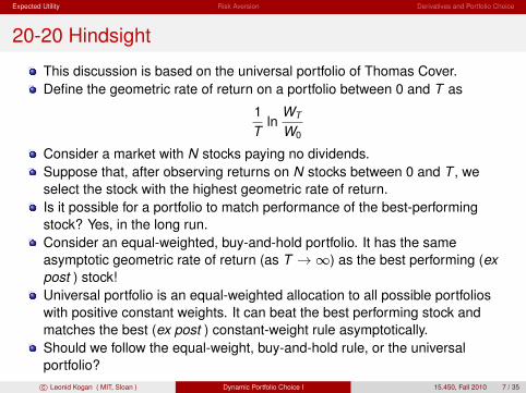
20-20 Hindsight

This discussion is based on the universal portfolio of Thomas Cover. Define the geometric rate of return on a portfolio between 0 and T as

1 WTlnT W0

Consider a market with N stocks paying no dividends. Suppose that, after observing returns on N stocks between 0 and T , we select the stock with the highest geometric rate of return. Is it possible for a portfolio to match performance of the best-performing stock? Yes, in the long run. Consider an equal-weighted, buy-and-hold portfolio. It has the same asymptotic geometric rate of return (as T ∞) as the best performing (ex →post ) stock! Universal portfolio is an equal-weighted allocation to all possible portfolios with positive constant weights. It can beat the best performing stock and matches the best (ex post ) constant-weight rule asymptotically. Should we follow the equal-weight, buy-and-hold rule, or the universal portfolio? c Dynamic Portfolio Choice I 7 / 35 � Leonid Kogan ( MIT, Sloan ) 15.450, Fall 2010


Where is the Catch

It is hard to have a meaningful discussion of which portfolio rules arepreferable without an explicitly specified objective.

Both of the portfolio rules described above may have nice asymptotic properties, but at any finite time point T they may produce return distributions with too much risk.

Consistent decision making under uncertainty can be based on the concept of expected utility.

Expected utility is not a dogma: it is based on behavioral assumptions.

Expected utility assumes rational, consistent choices.

Empirically, people often violate expected utility axioms.

No surprise there, people often behave irrationally.



The Framework

Define preference over random payoffs (gambles, lotteries), e.g.,

[$1000(0.5), $0(0.5)] vs. [$2000(0.3), $200(0.7)] � �� prob. prob. prob. prob.

Preferences are over outcomes only, e.g., do not depend on the mechanism by which cash flows are generated. Can apply to portfolio choice. � y (prefer �x to y� ), x� ∼ �y (indifferent between x� and �y )x � �Expected Utility Theory is a mathematical representation of preferences

� y E[U(�x)] > E[U(y�)]x � � ⇔

When we evaluate a random payoff �x , we care only about the numericaldistribution of cash flows: E[U(�x)].Properties of preferences are captured by the shape of the utility function U(x).

c Dynamic Portfolio Choice I 9 / 35 � Leonid Kogan ( MIT, Sloan ) 15.450, Fall 2010


Outline

1

2

3

Expected Utility

Risk Aversion




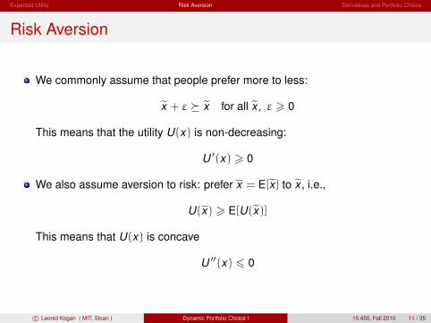
Risk Aversion

We commonly assume that people prefer more to less:

� x x , ε � 0x + ε � � for all �This means that the utility U(x) is non-decreasing:

U �(x) � 0

We also assume aversion to risk: prefer x = E[�x ] to x�, i.e.,

U(x) � E[U(�x)] This means that U(x) is concave

U ��(x) � 0



Risk Aversion

1 1.2 1.4 1.6 1.8 2 2.2 2.4 2.6 2.8 39.6

9.65

9.7

9.75

9.8

9.85

9.9

9.95

10

10.05

x

UU(E[x])



Risk Aversion

1 1.2 1.4 1.6 1.8 2 2.2 2.4 2.6 2.8 39.6

9.65

9.7

9.75

9.8

9.85

9.9

9.95

10

10.05

x

UU(E[x])

E[U(x)]



Coefficient of Relative Risk Aversion γ(W )

Start with initial wealth W . Compare two gambles, with payoffs

W (1 + x) and W (1 + xCE ), xCE is a constant

What value of xCE makes the agent indifferent?

Small gamble x . Use Taylor expansion around W (1 + x):

U(W (1 + x)) ≈ U(W (1 + x)) + U �(W (1 + x))W (x − x)+

1 U ��(W (1 + x))W 2(x − x)2 +

2 · · ·

U(W (1 + xCE )) ≈ U(W (1 + x)) + U �(W (1 + x))W (xCE − x)

Indifference implies

E [U(W (1 + x))] = U(W (1 + xCE ))

1U �(W (1 + x))Wx + U ��(W (1 + x))W 2Var(x) ≈ U �(W (1 + x))WxCE2

c Dynamic Portfolio Choice I 13 / 35 � Leonid Kogan ( MIT, Sloan ) 15.450, Fall 2010


Coefficient of Relative Risk Aversion γ(W )

Certainty-Equivalent Return

xCE ≈ x − 1 2 γ(W (1 + x)) Var(x), where γ(W ) = −

U ��(W )W U �(W )



Examples of Utility Functions

Linear utility U(W ) = a + bW , b > 0

implies that γ(W ) = 0. Payoffs are compared by their expected value, linear utility implies risk neutrality. Exponential utility

U(W ) = − exp(−aW ), a > 0

Assume W ∼ N(µ, σ2). Then � �2σ2aE [U(W )] = − exp −aµ +

2

Payoffs are compared by σ2

µ − a 2

Increasing relative risk aversion

γ(W ) = aW


�


Examples of Utility Functions

Constant relative risk aversion (CRRA) utility exhibits

γ(W ) = γ

Using the definition γ(W ) = −U ��(W )W /U �(W ), recover the utility function

1 W 1−γ , γ = 11−γU(W ) = �

ln W , γ = 1

CRRA utility is a very popular choice because of its implications for portfolio strategies.



Outline

1

2

3

Expected Utility

Risk Aversion



�


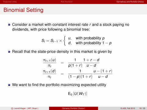
Binomial Setting

Consider a market with constant interest rate r and a stock paying no dividends, with price following a binomial tree:

u, with probability pSt = St−1 × d , with probability 1 − p

Recall that the state-price density in this market is given by

πt+1(u) 1 1 + r − d =

πt p(1 + r) u − d πt+1(d) 1 u − (1 + r)

= πt (1 − p)(1 + r) u − d

We want to find the portfolio maximizing expected utility

E0 [U(WT )]


��


Main Idea

t = 0 t = 1 t = 2

��

s1

�� s2

s3 ��

��

s4

Imagine that any possible state-contingent claim with payoff at T = 2 can be traded. Then portfolio choice is a simple static optimization problem: choose the claim WT

�(s) producing the highest expected utility subject to the budget constraint. Any state-contingent claim can be replicated by trading dynamically in the stock and the bond, therefore our optimal choice for WT

�(s) can be generated by dynamic trading.

c Dynamic Portfolio Choice I 19 / 35� Leonid Kogan ( MIT, Sloan ) 15.450, Fall 2010

� �


CRRA Utility Formulation

Suppose our objective is to maximize

E0 1 − 1 γ

WT 1−γ

starting with W0.

We look for the best state-contingent wealth allocation WT (s) that costs W0

at t = 0.

Recall that the time-0 value of any cash flow can be computed using the SPD as �

W0 = Prob0(s)πT (s)WT (s) s

Solve the static problem

max �

Prob0(s) 1

1 − γ WT (s)1−γ s.t.

� Prob0(s)πT (s)WT (s) = W0

s s


� �

�


CRRA Utility Solution of the Static Problem

Solve the static problem

max �

Prob0(s) 1

WT (s)1−γ s.t. �

Prob0(s)πT (s)WT (s) = W0 {WT (s)} 1 − γ

s s

Relax the constraint with a Lagrange multiplier λ

� 1 � max Prob0(s) WT (s)1−γ − λ Prob0(s)πT (s)WT (s) − W0

{WT (s)} 1 − γ s s

First-order optimality conditions

WT �(s)−γ = λπT (s) WT

�(s) = (λπT (s))−1/γ ⇒

Find the multiplier from

Prob0(s) (λπT (s))−1/γ

πT (s) = W0 s



CRRA Utility Solution of the Static Problem

We conclude that the optimal choice of time-T state-contingent cash flow is

WT �(s) = �

W0 πT (s)−1/γ

Prob0(s)πT (s)1−1/γ s

The recombining binomial tree model has a special property that the SPD is a function of the terminal stock price.

If the terminal stock price equals

ST = S0u(# Up moves)d(T −# Up moves)

then the SPD in the same state equals

πT = π1(u)(# Up moves)π1(d)(T −# Up moves)

1 1 + r − d 1 u − (1 + r)π1(u) = , π1(d) =

p(1 + r) u − d (1 − p)(1 + r) u − d



CRRA Utility Dynamic Trading Strategy

We were able to express the optimal state-contingent portfolio value at the terminal date, WT

�(s), as a function of the terminal stock price, denoted as

WT �(s) = H(ST (s))

The optimal portfolio must replicate the European derivative security with terminal payoff H(ST ).

We know how to construct the optimal trading strategy in the stock and the bond: it is the replicating strategy for the above derivative. Can compute it by backward induction.



CRRA Utility State-Contingent Allocation

Qualitatively, want to achieve higher wealth in states with lower SPD (higher stock price).

Illustrate by plotting the analytical solution from B-S framework (below).

ST

W* T

γ = 1

ST

W* T

γ = 4



Discussion

In the binomial setting, finding an optimal dynamic portfolio strategy reduces to figuring out which derivative security we would like to buy with initial wealth W0.

The static problem is easy to solve using a Lagrange multiplier.

Since any derivative can be replicated by dynamic trading in the stock and the bond, we know how to construct the optimal dynamic strategy for any utility function (e.g., proceeding backwards on the tree).



Black-Scholes Framework

Black-Scholes framework is a continuous-time limit of a recombining binomial tree, and dynamic portfolio choice is equally simple.

The advantage of continuous time is that we can obtain transparentclosed-form solution.

We use the B-S framework to recover the famous Merton’s solution to the dynamic portfolio choice problem.

Assume interest rate r and the stock price process

dSt = µ dt + σ dZtSt

We are performing calculations under the physical probability measure, so Zt = Zt

P .


� �

� �


CRRA Utility Static Problem

In analogy with the binomial-tree setting, we replace the dynamic problem with a static problem

max E0 1

WT 1−γ subject to E0 [πT WT ] = W0

{WT } 1 − γ

Keep in mind that WT and πT are both functions of the state, which is the entire trajectory of the Brownian motion between 0 and T .

Relax the constraint using a Lagrange multiplier λ:

max E0 1

WT 1−γ − λ (πT WT − W0)

{WT } 1 − γ

First-order optimality conditions

(WT �)−γ = λπT WT

� = (λπT )−1/γ ⇒


� �


CRRA Utility Static Problem

We find the multiplier from the static budget constraint:

E0 [πT WT �] = W0 E0 πT (λπT )

−1/γ = W0⇒

Find λ−1/γ = � W0 �

E0 πT 1−1/γ

We need to derive the dynamic strategy replicating the optimalstate-contingent claim WT

� .

We first derive the process for the optimal portfolio value, Wt �, and then figure

out how to delta-hedge it using the stock.


� �


CRRA Utility Dynamic Strategy

If the optimal portfolio value at T is given by Wt �, by DCF formula, portfolio

value at earlier times must be equal to

Wt � = Et

πT WT � , WT

� = (λπT )−1/γ

πt

Recall that in the Black-Scholes model, the price of risk is constant, η = (µ − r)/σ, and the SPD is given by

πt = e−rt e−(η2 /2) t−η Zt

We can compute Wt �: � � � � �1−1/γ

�

W � λ−1/γπ−1/γ πT

λ−1/γ πT π−1/γ

t = Et T = Et tπt πt

= F (t)π−t

1/γ

for some function of time F (t), which we could compute explicitly.



Dynamic Strategy

To figure out the dynamic trading strategy, we relate the SPD to the stock price, just like we did for binomial tree.

The SPD is given by πt = e−rt e−(η2 /2) t−η Zt

The stock price equals St = S0e(µ−σ2/2) t+σ Zt

We conclude that πt = G(t)St

−η/σ

for some function G(t). We can compute G(t) explicitly but do not need to.

The optimal portfolio follows

W � = F (t)G(t)−1/γSη/(γσ) t t


�

�

� �

�

� �

�

�


Dynamic Strategy

Let θt denote the optimal number of stock shares in the dynamic portfolio.

tDefine φ to be the weight of the stock in the optimal portfolio:

θt St

Wφ = t

t

Delta-hedging rule tells us how many stock shares to include in the replicating portfolio

Using

∂Wtθ = t ∂St

= F (t)G(t)−1/γSη/(γσ) tWt

we conclude that φ

η µ − r = = t γσ γσ2



Dynamic Strategy

Merton’s Solution In the Black-Scholes setting with CRRA utility function, the weight of the stock in the optimal portfolio is

φ� t =

µ − r γσ2

Merton’s solution says that the optimal portfolio weights are constant,independent of the problem horizon T .We call such solution myopic. It is optimal to behave as if the horizon of the problem is very short. The optimal weight of the stock is increasing in the risk premium, anddecreasing in relative risk aversion and stock return volatility.For a general utility function, U(WT ), we would not obtain the same solution, optimal portfolio strategy would not be myopic. CRRA utility is special: constant relative risk aversion. This, combined with the fact that returns on all assets in the B-S model are IID, leads to a myopic optimal portfolio. c Dynamic Portfolio Choice I 32 / 35 � Leonid Kogan ( MIT, Sloan ) 15.450, Fall 2010


Merton’s Solution

Merton’s solution easily generalizes to a multi-variate case. If an investor has a CRRA utility function, interest rate is constant, r , and returns on N risky assets follow

NdSti

= µi dt + �

Σij dZtj ,

Sit j=1

then the vector of optimal portfolio weights on the N stocks is given by

φ� = 1 (ΣΣ �)

−1 (µ − r1)t γ

where µ = (µ1, ..., µN )�, 1 = (1, 1, ..., 1) �, and ⎤⎡ ⎢⎢⎣

Σ11 Σ12 . . . Σ1N

Σ21 Σ22 . . . Σ2N ⎥⎥⎦Σ = . . .

ΣN1 ΣN2 . . . ΣNN



Summary

Need a coherent objective to formulate an optimal dynamic trading strategy: Expected Utility Theory.

In a setting in which all state-contingent claims can be replicated by dynamic trading (e.g., binomial tree, Black-Scholes model) can connect optimal portfolio choice to option pricing.

In the Black-Scholes setting with CRRA preferences, the optimal portfolio strategy is myopic, given by the Merton’s solution.



References

T. Cover, 1991, “Universal Portfolios,” Mathematical Finance 1, 1-29.


MIT OpenCourseWarehttp://ocw.mit.edu

15.450 Analytics of Finance Fall 2010

For information about citing these materials or our Terms of Use, visit: http://ocw.mit.edu/terms .

http://ocw.mit.edu

http://ocw.mit.edu

Documents

Dynamic Portfolio Choice I - MIT OpenCourseWare · PDF fileDynamic Portfolio Choice I Static Approach to Dynamic Portfolio Choice Leonid Kogan MIT, Sloan 15.450, ... 15.450 Analytics