Polyspectral analysis of mixed processes and coupled harmonics

IEEE TRANSACTIONS ON INFORMATION THEORY, VOL. 42, NO. 3, MAY 1996 943

Polyspectral Analysis of Mixed Processes and Coupled Harmonics

Guotong Zhou, Member, IEEE, and Georgios B. Giannakis, Senior Member, IEEE

Abstract-Polyspectral analysis of processes with mixed spectra is considered, and scaled polyperiodograms are introduced to clarify issues related to stationarity, ergodicity, and suppression of additive stationary noise in harmonic retrieval problems. Spectral and polyspectral approaches are capable of retrieving (un)coupled harmonics, not only when the harmonics have constant amplitudes, but also when they are observed in nonzero mean multiplicative noise. Fourier series polyspectra and asymptotic properties of scaled polyperiodograms provide general tools for higher order analysis of time series with mixed spectra. A single record phase coupling detector is derived to obviate the assumption of independent multiple records required by existing methods. The novelties are illustrated by simulation examples.

Zndex Terms-Frequency- and phase-coupled harmonics, multiplicative noise, polyspectra, asymptotic properties, ergodicity.

I. INTRODUCTION

ETECTION and estimation of processes with mixed D spectra is well-documented in time series analysis and has found widespread applications in signal processing. They can be modeled as discrete-time complex harmonics-in-noise processes

L

s(t) = ~ ( t ) + ~ ( t ) = A Z ~ ~ ( ~ ‘ ~ + $ ‘ ) + v ( t ) , 1=1

t = 0,1, . . . , T - 1 (1)

and their spectra are mixed in the sense that they consist of lines superimposed on the smooth spectrum of the stationary noise v ( t ) .

Second-order analysis of mixed processes remains an active research area to date, but recently there has been a revived interest toward higher order spectral, and in particular bispectral, analysis. The primary motivation in this context has been the ability of bispectra to discern quadratic frequency coupling. The latter appears in (1) when there exist inte- ger triplets ( Z l , b 2 , 1 3 ) E [1,L] such that wzl + wlZ = w13. Coupled frequencies show up when harmonic components

Manuscript received January 3, 1994; revised December 10, 1995. This work was supported by ONR under Grant N00014-93-1-0485. Some results of this paper were presented at the Asilomar Conference on Signals, Systems and Computers, Pacific Grove, CA, November 1993.

G. Zhou is with the School of Electrical and Computer Engineering, Georgia Institute of Technology, Atlanta, GA 30332-0250 USA.

G. B. Giannakis is with the Department of Electrical Engineering, Univer- sity of Virginia, Charlottesville, VA 22903-2442 USA.

Publisher Item Identifier S 0018-9448(96)02909-4.

interact nonlinearly and bispectral approaches for detecting such interactions have been reported in oceanography [I], seismology [ 2 ] , EEG analysis [3] , manufacturing [4], laser velocimetry [5] , and plasma physics applications [6].

On the other hand, both frequency and phase coupling may incur in a harmonic process; namely, there may exist integers 11 ,12 ,13 E [l, L] such that both wll + wlZ = w13 and 4z1 + q h 1 2 = 4z3 are satisfied. Although frequency coupling alone may be coincidental, frequency and phase coupling together is a strong indication of possible nonlinearities. As an example, consider complex exponentials like

undergoing a linear-quadratic transformation such as y ( t ) = u( t ) + au2(t). As a result, y ( t ) contains harmonics with frequencies 2wl,2w2, and w1+ w2, with corresponding phases 2 4 1 , 2 4 ~ , and qhl + 4 2 , besides those already present in u(t) . In this context, Kim and Powers [6] and, more recently, Nikias and Raghuveer [7], [SI, [9], have developed nonparametric and parametric bispectrum-based coupling detectors assuming that the phases are random and uniformly distributed in ( - T , T].

With regard to frequency estimation, Brillinger [ 101 was the first to compare spectral with bispectral approaches for coupled harmonics. More recently, Swami and Mendel [ 111-[ 131 dealt with coupled and uncoupled harmonics and motivated fourth-order cumulant-based harmonic retrieval as a means of “suppressing” additive colored Gaussian noise. Cumulant- based high-resolution methods for retrieving quadratic phase coupling have also been reported in [ 141.

The present paper offers a framework for polyspectral analysis of mixed processes in general, and develops novel results for detecting frequency- and phase-coupled harmonics in particular. The pioneering work of Brillinger-Rosenblatt [U] for mixing processes is extended to mixed processes. The following assumptions are made regarding the model in (1):

a l ) Al’s are real, nonzero, and deterministic constants. a2) 42’s are deterministic constants in ( - T , T ] .

a3) wl’s are distinct in ( - T , O ) U ( 0 , ~ ) . a4) v( t ) is zero-mean, stationary, with ( k + 1)st-order

cumulants

0018-9448/96$05.00 0 1996 IEEE

944 IEEE TRANSACTIONS ON INFORMATION THEORY, VOL. 42, NO. 3, MAY 1996

satisfying [16, p. 261

We adopt the notation ~ ( ~ % ) ( t ) to signify v ( t ) if p , = 1 and v * ( t ) if p , = -1, and require p , E (-1, l}. Since the vector p = bo,. . . , p k ] can take 2kt1 values, condition (2) implies that all 2‘“+l possible ( k + 1)st-order cumulants of v( t ) defined with different conjugations in the lagged copies of v(t) are absolutely summable. We refer to (2) as the mixing condition [16, p. 91 and to processes satisfying (2) as mixing processes. We remind the reader that mixing processes are inherently different from processes with mixed spectra, and the terms “mixing” and “mixed” should not be confused.

The absolute cumulant summability as in (2) implies that samples of v ( t ) which are well separated in time can be regarded as approximately independent. Signals satisfying (2) include linear and nonlinear processes of the Volterra type with stable (i.e., absolutely summable) kernels [ 16, Theorems 2.8.1, 2.9.11. Moreover, we infer from (2) that ( k + 1)st-order polyspectra of w ( t )

A

A. (BijSpectra of Stationary and Mixing Processes-A Review

A zero-mean and stationary process w ( t ) has time-invariant second- and third-order cumulants/moments

Under a4), its spectra and bispectra are well-defined as the Fourier transforms (FT) of (3) and (4), respectively

CO

T = - m

CO 00

r1=-m r2=-00

The following alternative definitions can be shown to be equivalent to ( 5 ) or (6):

(7)

exist and are finite, since Equations (7) and (8) suggest the following sample estimates:

In Section I1 we introduce Fourier series polyspectra and scaled polyperiodograms as their natural estimators, and prove that additive noise need not be Gaussian for harmonic retrieval. Statistical properties of scaled polyperiodograms are established, and generalizations are made to nonzero mean multiplicative noise models. We argue in Section I11 that contrary to what is assumed in [7]-[9], phase-randomized harmonics are not ergodic in their scaled polyperiodograms. Moreover, frequency coupling alone is sufficient for scaled polyperiodograms to peak. A novel phase coupling detector is derived in Section IV to obviate the restrictive requirement of existing methods [61-[9] for multiple independent records. Section V is devoted to simulations to illustrate the main points of the paper, and conclusions are drawn in Section VI. Proofs are collected in the Appendix.

11. FOURIER SERIES POLYSPECTRA AND SCALED POLYPERIODOGRAMS

We start with conventional polyspectra and polyperiodograms for stationary and mixing processes, and show that existing definitions are inappropriate for processes with mixed spectra. In [15], [16], the focus has been on mixing processes.’ Note however, that harmonics-in-noise do not satisfy (2).

A 1 13c(Xl; X2) = ~ v T ( ~ l ) V T ( ~ Z ) v ~ ( ~ l f X2). (10)

The quantities in (9) and (10) are termed periodogram and bi-periodogram, respectively, and are asymptotically unbiased but inconsistent estimates of (7) and (8). However, consistency can be established with appropriate averaging windows [ 151,

B. FS Time-Averaged Moment Polyspectra

Although (bi)spectral estimation of stationary and mixing processes is by now well-understood, (bi)spectral analysis of processes with mixed spectra has not been investigated thoroughly. For example, under a2), ( 5 ) is not well defined for the multitone model of (l), because E{z*( t ) z ( t + T)} is generally time-varying, and so is the bispectrum in (6).

For nonstationary processes like the z ( t ) of (l), the ex- pectations in (3) and (4) are time-varying. Generalizing to ( I C + 1)st-order moments, let us define

a m(k+l)z(t;C = Jq z*( t ) z ( t + 71). . . z( t + T k ) } . (11)

To remove the t-dependence, we time-average m(,+l)z(t; T)

to obtain2

(12) a 1

t=O ‘In [16, p. 1721, assuming uniform random phases, (1) was only briefly

noted as “departure from assumptions.” 20verbar is used in this paper to denote time-averaged quantities

ZHOU AND GIANNAKIS: POLYSPECTRAL ANALYSIS OF MIXED PROCESSES AND COUPLED HARMONICS

where for the x ( t ) of (1) the limit exists for each fixed T (see also [17, p. 281). Definition (12) subsumes the stationary case because the limiting average operation drops for time-invariant moments and TE(~+~)=(T) = m ( k + l l z ( ~ ) . The natural estimator of m(k+l) , (~) is the sample average

where 6(.) denotes the Kronecker delta function

1, X = 0 mod (27r) S(X) = a { 0, otherwise.

Note that the following identity is used in deriving (15):

~ T-1

Under the deterministic phase assumption a2), ~ ( t ) of (1) is cyclostationary in the sense that m ( k + , ) z ( t ; ~ ) is an (almost) periodic sequence in both t and 7, 'dk [18] (see also [19] for a thorough treatment of (uniformly) almost periodic functions). But even under the usual randomized phase assumption which stationarizes the process, 7E(k+l), (T) is an (almost) periodic sequence in T. Therefore, in both cases, the exp { j w ~ } factors such as those in (14) or (15) are not absolutely summable, and hence the FT of T E ( k + l ) z ( ~ ) is not well defined unless one introduces Dirac delta functions [16, p. 1731. However, the fact that exp { j w ~ } is an (almost) periodic sequence of 7

prompts us to consider instead, the (generalized) Fourier series (FS) coefficient of m ( k + 1 ) , ( ~ )

. T--1

where the summation over r is understood as being k-fold. Moments, as opposed to cumulants, are considered here be-

cause except for the mean, cumulants of additive deterministic quantities vanish, and thus the harmonics of interest disappear in cumulant domains. For succinctness of terminology, we henceforth call (1 8) the FS polyspectrum, while its full name could have been the generalized FS time-averaged moment polyspectrum.

The k-dimensional FS coefficient in (18) is called generalized because it applies even to almost periodic sequences [ 171,

945

[ 181. For discrete-time strictly periodic signals with period N , the classical FS expansion, e.g., with k = 1

N-1

n = O

applies only when w, = 27rn/N with n,N E Z . The FS coefficient

N-1

r = O

is subsumed in the definition T-1

The latter holds even for X # w, = 27rn/N which corresponds to almost-periodic signals with frequencies not on the FFT grid.

Substitution of (1 1) and (1 2) into (1 8) reveals an equivalent definition of x ( k + l ) z ( A )

x x;(& + . . . + Ak). (19)

A natural estimator of (19) is given by the ( k + 1)st-order scaled polyperiodogrum

x X ; ( A 1 + ' . . + X k ) (20)

which is T-k times the usual (A: + 1)st-order polyperiodogram

A 1 ~ ( k + l ) , ( ~ ) = TXT(X1) . ' . - k ; T ( X ~ ) X ~ ( X l + . . . + X k ) . (21)

It is obvious from (19) and (20) that %?(k+l)z(A) is an asymptotically unbiased estimator of M(k+l)z (A)

Note that no windowing is necessary since we are dealing with harmonics, and as we see later on, even in its raw form, (20) is consistent at the frequencies of interest. Scaled biperiodograms for mixed processes were also alluded to in [lo], and will become clear in the sequel. First, FS polyspectra help us to clarify claims regarding theoretical insensitivity of higher order spectra to Gaussian noise.

C, Harmonics in (Non-)Gaussian Additive Noise

In a laser Doppler velocimetry experiment, Sat0 et al. advocated the usage of bispectra over spectra, due to the ability of the former to "suppress" additive Gaussian noise [SI (see also [20]). The same argument has been used repeatedly in many recent papers dealing with cumulant-based retrieval of uncoupled and coupled harmonics [5]-[9], [I 11, [131, [141. Indeed, cumulants and polyspectra of order 2 3 theoretically vanish when v ( t ) in (1) is Gaussian. But as we prove subse- quently, for harmonics-in-noise processes, any w( t ) satisfying


a4) has the same asymptotically vanishing contribution to z(k+l)z (A), irrespective of its dis t r ibut i~n,~ which includes even the second-order quantity a,z(A) . We establish the latter by first noting that the FS of (14) is given by

Due to the mixing condition (2), we find that

I . T-1 I . T-1

and hence the second term on the r.h.s. of (23) is zero. We thus infer

L

Z z z ( X ) = CA:S(X - w1). (24)

Equation (24) shows that z z z (A) is theoretically insensitive to any stationary and mixing noise. This result can be further understood if instead of (19), one adopts definition (7). The spectrum Szz (A) then exhibits infinite (Dirac) peaks superimposed on a smooth and finite spectral floor &,(A) [16, p. 1731; whereas in (24), Kronecker deltas occur at the wl ’s and T-’Sp,(X) in (23) tends to zero as T i x.

By the same token, (2) ensures that the FS of (15) is given by (c.f. (18) with k = 3)

1=1

L

Z3,(X,. X p ) = A1,Al ,A1,e3(d’ l+~12-~13) l i , l ~ , 1 3 = 1

x 6(X1 - w1,)S(A2 - W 1 3 )

x qw1, + w/a - U/,). (25)

Note that in deriving (25), we only needed

71,72

and did not assume that c g , ( ~ 1 , ~ 2 ) = 0; which reiterates the fact that any noise satisfying (2) can be tolerated when retrieving harmonics. The last delta in (25) requires wl, + w12 = w13 for %3z(A1, A,) to be nonvanishing; i.e., quadratic frequency coupling is necessary for the FS bispectrum to be nonzero. Under this condition, the first two deltas imply that M,,(Xl, A,) peaks at the bifrequencies (wI1 U / * ) .

Extending (25) to ( k + 1)st-order scaled polyperiodograms, it is straightforward to show that

~

x S(A1 - wl) . . . &(AI, - W E )

x qwz, + . ‘ . + (26) -

’In practice and with finite data records, noise contribution generally depends on its distribution. However, Gaussian noise “insensitivity” claims which rely on the asymptotically vanishing bias of sample cumulants should also take into account their high sample variance.

Therefore, only when kth-order frequency coupling is present

k c W L = i=l

the ( k + 1)st-order FS polyspectrum is nonzero and peaks at ( w l l . . . win). In fact, among polyspectra, kth-order couplings can be and can only be detected from the peaks of ( k + 1)st- order polyspectra (see also [ 111).

D. Scaled Polyperiodograms-Asymptotics

In Section 11-B, we introduced scaled polyperiodograms as natural estimators for FS polyspectra. The next theorem summarizes asymptotic properties of scaled (bi)periodograms. We focus on second- and third-order quantities first, because they are more frequently encountered in practice.

Theorem I : If z ( t ) is given by (1) and al)-a4) hold, then the asymptotic variance of the scaled periodogram peak at wl

is given by

lim Tvar { a p z ( w l ) } = 2A;S2,(w1). V1 (27)

where SzC(A) denotes the power spectral density of v ( t ) . If L = 3 and w1 + w2 = w3, we have three cases for the asymptotic variance of the scaled biperiodogram peak at

c l ) when w1 # -2w2 mod (27r), and wp # -2wl mod (27r)

T - x

(&I. wp):

lim T var {%3z (“1, w z ) } = A;A;s~, (w1) T-32

+ A::A%V(W3) + A::A;S2&2) (28)

c2) when w1 = -2wzmod(27r)

c3) when w2 = -2wlmod(27r)

Pro03 See Subsection A in the Appendix. The next theorem generalizes the scaled biperiodogram

results to ( k + 1)st-order scaled polyperiodograms, where asymptotic normality is also established.

a We remind the reader that var {z} = cov { x, z} = cum {z*, .z} # cum { z, z} for z complex

ZHOU AND GlANNAKIS: POLYSPECTRAL ANALYSIS OF MIXED PROCESSES AND COUPLED HARMONICS

~

947

Theorem 2: Let x ( t ) be given by (1) and assume that al)-a4) hold. If the frequencies in (1) are kth-order-coupled,

IC

Wk+l = wa a = l

and satisfy

then with w 5 ( w l , . . . , w k ) , we have that f i % ( k + l ) z ( W )

and flx(k+J)z ( w ) are jointly asymptotically normal with asymptotic variance at the scaled polyperiodogram peak given by

* *

and

Proof: See Subsection B in the Appendix. Note that we only discuss asymptotic properties at the

scaled polyperiodogram peak, because these quantities are needed later on for developing phase coupling detectors. The properties off the peaks are not of interest in this paper. In fact, they follow (within a scalar) asymptotic properties of polyperiodograms of stationary and mixing processes which have been thoroughly treated in [ 151.

Although most of the results of this paper can be extended to ( k + 1)st-order moments without difficulty, we henceforth focus only on third-order quantities due to space limitations.

E. Extensions to Multiplicative Noise Models

When harmonics propagate through dispersive media (e.g., the ocean), are reflected from scintillating targets, or are trans- mitted through fading channels, multiplicative noise effects occur [21]-[24]. Under these circumstances, we can remodel (1) as

l.= 1

t = 0,1, . . . , T - 1. (34)

Besides a2)-a4), we also assume: a5) sl(t)’s satisfy (2), and are real, stationary, with nonzero

means m.l, independent of each other, and independent of v ( t ) . We can regard (1) as a special case of (34) by letting

s l ( t ) Al. With respect to (34), we will show that when quadratic frequency coupling is present, the FS bispectrum again peaks at the bifrequencies. This result along with the asymptotic properties of =32 ( w l , wz) are summarized next:

Theorem 3: If x ( t ) is given by (34), satisfies a2)-a5), and wll + w12 = w l j mod (27r) holds true only for Zl # l 2 # Z 3 , then we have that

l 1 , b , l 3 = 1

x S(X1 - Wl1 )S(X2 - W l a )

x q w l , + U/% - W 1 3 ) (35)

where ml = E(s l ( t ) } . If L = 3 and w3 = w1 + w2, then

f i % 3 z ( w 1 , w 2 ) and fi%3z(wl, w2) are jointly asymptotically normal, with asymptotic variance at the peak given

A A *

by

and

where SZsL(X) is the power spectrum of s l ( t ) . Proof: See Subsection C of the Appendix.

Note that if we treat (1) as a special case of (34) with s l ( t ) = Al, then ml = Al , caS l ( . r ) = 0,S2sl(X) = 0, and (35)-(37) reduce to (25), (28), and (31), respectively.

Theorems 1-3 not only have their own importance in terms of performance evaluation of scaled polyperiodograms for processes with mixed spectra, but also lead to important phase coupling detection algorithms to be discussed in Section IV.

111. FREQUENCY- AND PHASE-COUPLED HARMONICS

Under the standard separation condition (min I&, - Gn I = TP1/’,m # n), and similar to [lo], (24) can be used to estimate the harmonic frequencies by searching for the L greatest maxima in the scaled periodogram

L A

(38) L { ~ z } l = ~ = a r g m a x C Z 2 , ( X i ) .

The frequency estimators have been shown to be consistent with variance converging to zero at an O ( T P 3 ) rate5 [lo]. Once frequency estimates are available, amplitudes can be consistently estimated according to (24) as

X l , . . . , X L

A; = x2z(ijjl). (39)

Potential quadratic frequency coupling can be verified by first obtaining { i j l } f = l from (38), and then searching exhaustively for frequency triplets {ijll, G12, & 1 3 } such that ijzl + & 1 2 = ijls

5By h(T) ,= O ( T k ) we mean that limT,, h ( T ) / T L = e where the L <cw. constant c satlsfies 0 < I ,I


statistically (meaning that for a given false alarm rate the null hypothesis &lI + ijld - ij13 = 0 is accepted). In principle, since all frequency estimates are available, kth-order frequency couplings can be detected from Z2,(X) by searching for (11, . . . , Zk+l} such that + . . . + Lqk = i j l k + l statistically, for any k .

An alternative way of checking for quadratic frequency coupling can be derived from (25), which bypasses the afore- menconed cumbersome exhaustive search. Presence of peaks in la,, ( XI, A,) I indicates quadratic frequency coupling and bifrequency estimators can be obtained from

(41,42) = argmaxIM3,(X1.X2)1. (40) A 1 ,A2

The estimators in (40) have been shown to be consistent with computable variances [IO]. It is interesting to note that Brillinger in [IO] did not assume that w ( t ) is Gaussian, which corroborates our proof in Section 11-C that (bi)periodograms can retrieve harmonics without regard to the noise distribution. However, in [20], Brillinger acknowledged the work by Sat0 et al. [5] which favored the use of bispectra based on their ability to “eliminate” additive Gaussian noise only.

Using bispectra to detect quadratic frequency coupling in ocean wave interaction was first performed by Hasselman et al. in [l]. In [6], Kim and Powers employed frequency coupling to detect nonlinearities present in plasma fluctuation data. But more recently, Nikias and Raghuveer [7]-[9] advocated bispectra for detecting not only frequency but also phase coupling, as a means of “double-checking” for presence of nonlinearities. In [7]-[9], the phases were assumed to be uniformly distributed in ( -T, T ] and when dealing with sample estimation, ergodicity was assumed which as we show next is incompatible with the phase randomization assumption.

If (apart from coupling) the 41 ’s in (1) are assumed to be independent and uniformly distributed in ( -T. T ] (denoted as - U ( - x , T I ) , then mimicking the steps used in deriving (25) , one arrives at (see also [71-[91)

which renders that z ( t ) is m.s.s. nonergodic with respect to its third-order statistics. Lack of ergodicity was also mentioned in [ 111 and can be easily understood if we view the complex exponential in (41) as a random constant. It is well known that random constants are nonergodic [25, p. 2481; i.e., we cannot estimate the expected value of a random constant €rum its single record realization.

Multiple records with independent phase realizations are necessary to “restore” ergodicity, and after averaging over independent records, frequency-coupled harmonics which are also phase-coupled will peak. However, our phase coupling detector to be developed in the next section alleviates the requirement for independent multiple records, if the phases are viewed as deterministic.

IV. SINGLE RECORD PHASE COUPLING DETECTION

As we explained in Section 111, existing methods need independent multiple records and randomized phases to reveal phase coupling which may be true with snapshots collected at an array of sensors. A novel approach is developed here using a single record of data. The focus will be on the L = 3 case and quadratic coupling. Generalization to more complicated situations is straightforward using the results developed in Section 111.

Although frequency coupling alone is meaningful, as for example, in gear noise analysis [4] and laser Doppler velocimetry [5] where it is possible to input frequency-coupled harmonics, phase coupling alone is not so meaningful. Therefore, we pursue phase coupling detection only after the frequencies have been confirmed as being coupled. Coupled bifrequency estimates have variance 0 ( T 3 ) [lo], in contrast to coupled phase estimates which will be shown next to have variance O ( T - l ) . Such a small variance of ijl allows us to analyze performance of biphase estimates &GI, 22) by approximating them with &wl . w 2 ) as if the bifrequencies were known.

L A. Phase Estimates at Bispectral Peaks

Based on (25), let us define We focus on model (1) with L = 3 and w1 + wz = w3.

M3a:(X1, X2) = Ai,A”Al,E(e3(~’1+~’2-’’3) } 11,12,13=1

x S(X1 - wz1 )S(X2 - W l a )

4 A 41 + 4 2 - 4 3

d arg [ i?3T(u1,w2)1 = arctan(f/il) (43)

(42) x qwz, + Wiz - w 3 ) - (41)

Since E[exp {j4}] = 0 for q5 - U ( - T , T], we infer from (41) that both frequency and phase couplings, wl1 + w12 = w13 and

absence of phase coupling, one has that ~ 3 , ( ( w l 1 , w l 2 ) = 0. However, even under the randomized phase assumption, the phases take on fixed values throughout a given record anyway; hence, if only frequency coupling is present, one infers from (25) and Theorem 1 that

4 1 ~ + q512 = are necessary for (41) to be nonzero. In the A ^ where R + j i = M ~ , ( w ~ , w ~ ) . Equation (42) implies that if 41 + 4 2 = 4 3 ; the estimate 4 be to zero statistically. To perform the statistical test called for, we first postulate two hypotheses:

Ho: 4 = 0 versus H I : q5 # 0. (44) lim ~ ~ ~ , ( L L J ~ ~ , ~ ~ ~ ) ~ ,gs’ lAllA12A131 # 0.

T i m Statistics of 4 are necessary to perform the $est, which we

develop next. Since @ Z ~ Z ( ~ I , @M,,(wi, %) are jointly asymptotically normal by Theorem 2, and R , f are

linear combinations of Msz (w1 , w2) and z 3 2 ( w 1 , wz) , we infer that fig and are asymptotically normal as well.

We therefore reach a dichotomy; namely, that under the phase randomization assumption and with wL1 + w12 = wl3 but 411 + $ l a # 412, we have

A *

m.s.s. -

T-CC lim ~ 3 z ( w 1 , %) # M3,(Wl , W I Z ) = 0

ZHOU AND GIANNAKIS: POLYSPECTRAL ANALYSIS OF MIXED PROCESSES AND COUPLED HARMONICS 949

Next, by denoting Once I? is chosen, a threshold 7 = I’cri/T can be selected with a$ determined either from (46) or (48). Since

we obtain the following Taylor series expansion of the arctan ( i / k ) function in (43):

where higher than first-order terms in (k - R) and (1 - 1’) are omitted. Due to ( 4 3 f l 4 is also asymptotically normal. Furthermore, Theorems 1-3 lead to the following results:

Theorem4: If for the z ( t ) of (l), L = 3 ,w l + w2 = w3, w1 # -2w2 mod (ax), w2 # -2wl mod (ax) , and 4,$ are defined as in (42) and (43), then under a1)-a4), f l (4 - 4) is asymptotically normal N(0, a?), with asymptotic variance

4

we estimate $ from the data as in (43), and compare JZ with 7. If

In practice though, the threshold I needs to be estimated from a single record of data as well, which in turn, calls for estimates of 02. For the constant amplitude case, 02 can be estimated via (46), provided that one has estimates of A; and S2w(w1). From a single record, the former is estimated as in (39), whereas for the latter, we need to avoid the harmonic at w1 and average (smooth) periodogram ordinates as usual [ 16, p. 1731, in order to obtain a consistent estimator of the smooth spectrum of v(t) . For the random amplitude case, however, it is impossible to infer S2sl (A) needed in (48) from the periodogram. We then resort to cyclic algorithms as detailed in [22] and [261.

> 7, we reject H O .

4 dJ

V. SIMULATIONS

We present in this section numerical examples to verify and . illustrate our results on scaled biperiodograms and quadrati- cally coupled harmonics. The signal-to-noise ratio (SNR) is

If in addition ~ ( t ) is white with variance a;, then (46) simplifies to

defined in deciels as

T-1 (47)

Under the same assumptions for the z ( t ) of (34) but with

1 A AT (7,

3 1 SNRl = 7.

03 = 2 c 1=1 ” IY(t) I2

v 2 ( t )

(51) a

as) replacing al l , JT($ - 4) is also asymptotically normal SNR = 10logl, tT=_O1 n/(O,a2) 4 with asymptotic variance

t=O 2 1

0 - = -[Szw(w2) + S2s1(w2 - w1) + Szs,(wl)] 4 am; When colored, noise v ( t ) was generated from i.i.d. deviates

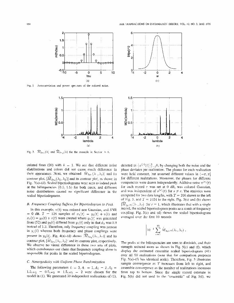
w ( t ) according to: v(t)-0.8253v(t-1)+0.25w(t-2) = w( t ) . Fig. l(a) and (b) shows the autocorrelation sequence and the power spectrum (5) of the colored noise w ( t ) . Moreover, when Gaussian (non-Gaussian) v ( t ) is referred to, the driving noise w ( t ) was Gaussian (one-sided exponentially) distributed. For computational convenience, scaled biperiodograms were formed by first segmenting the data into sub-records of length 64 each, calculating l\/r32(X1, A,) (c.f. (20)) for each sub- record and then averaging them. Only the first quadrant scaled biperiodograms and the corresponding peak contours are displayed here.

A. “Insensitivity” to Additive Stationary Noise

1

1

+ ! % f [ s z w ( w l ) + s2sz(w1 - w 2 ) + s2s’(wz)1

+ 7 [ s 2 w ( w 3 ) f s 2 s l ( w 2 ) f s2s,(w1)]. (48)

are white with variance d1 and

2m3

If in addition s l ( t ) and a;, respectively, then (48) becomes

. (49) 1 A m? 3

3 SNRl = 1 “$=,E,,:

4 + 4% 1=1

z=l,r#l

Proof: See Subsection D of the Appendix.

B. Statistical Test

Since f l (4 - 4) is asymptotically normal under Ho, we infer that TJ2/a2 is X2-distributed with one degree of freedom. For a prescribed false alarm rate PFA, a constant l- can be determined from a x2 (1) table so that

dJ

p,z (x) dx = PFA JI”’ where p,~(x) is the ~ ’ ( 1 ) density function.

We generated a 128-point frequency-coupled harmonic time series according to the model

and then added noises to form xl ( t ) = y ( t ) + w l ( t ) and 1 ~ 2 ( t ) = y ( t ) + wz(L), where wl(t) was colored Gaussian, and w z ( t ) was i.i.d. one-sided exponential. The SNR’s for x l ( t ) and x2( t ) were both at 0 dB. Fig. 2(a) and (b) shows the estimate of (24) for z l ( t ) and zz( t ) , respectively, cal-

950

6

- h ? 4. 3 I v

. . . . . . . . . . -

IEEE TRANSACTIONS ON INFORMATION THEORY, VOL. 42, NO. 3, MAY 1996

. . . . . . . . A .:. . . . . . . .:. . . . . . . . :. . . . . .

-2 . . . . . . . . ~. . . . . . . . . . . . . . . :.. . . .

4

-2 0 2 4 ‘14 -2 0 2 4 lambda lambda

(a) (b)

Fig. 2. mzSl(X) and a z z 2 ( A ) for the example in Section V-A.

culated from (20) with li: = 1. We see that different noise distributions and colors did not causeA much difference in their appearance. Next, we obtained 1%321 (A,, A,) I and its contour plot, 1x322 (AI, A,) I and its contour plot, as shown in Fig. 3(a)-(d). Scaled biperiodograms were seen to indeed peak at the bifrequencies (0.5, 1.5) for both cases, and different noise distributions caused no significant difference in the scaled biperiodograms.

B. Frequency Coupling Sufices for Biperiodogram to Peak

In this example, v ( t ) was colored non-Gaussian, and SNR = 0 dB. T = 128 samples of z l ( t ) = yl ( t ) + w ( t ) and z ~ ( t ) = y ~ ( t ) + w ( t ) were created where yl( t ) was generated from (52) and y 2 ( t ) differed from yl( t ) only in that 43 was 0.9 instead of 1.2. Therefore, only frequency coupling was present in y l ( t ) whereas both frequency and phase couplings were present in y,(t). Fig. 4(a)-(d) shows l g 3 2 1 (AI, X Z ) ~ and its contour plot, 1 z 3 2 2 (AI, A,) 1 and its contour plot, respectively. We observe no visual difference in these two sets of plots, which corroborates our claim that frequency coupling alone is responsible for peaks in the scaled biperiodogram.

C. Nonergodicity with Uniform Phase Randomization

The following parameters L = 3 , A l = l , A Z = 2,A3 = 1.5,wl = 0 . 5 , ~ ~ = 1 . 5 , ~ ~ = 2 were chosen for the model in (1). We generated 50 independent realizations of (l),

denoted as { ~ ( ‘ ) ( t ) } ~ = ~ 0 , by changing both the noise and the phase deviates per realization. The phases for each realization were held constant, but assumed different values in ( -T , 7r ]

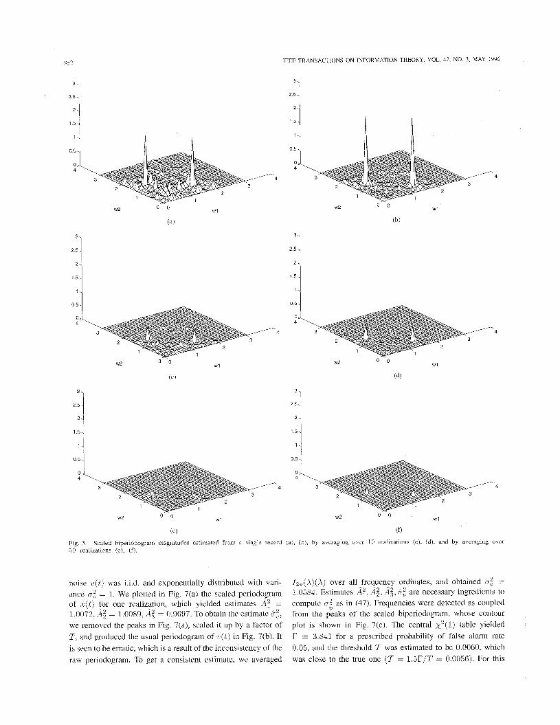
for different realizations. Moreover, the phases for different components were drawn independently. Additive noise ( t ) for each record r was set at 0 dB, was colored Gaussian, and was independent of d s ) ( t ) for s # T. The statistics were computed for two data lengths, with T = 256 shown to the left of Fig. 5, and T = 1024 to the right. Fig. 5(a) and (b) shows /B3z.1) ( A l . A2)1 for T = 1, which illustrates that with a single record, the scaled biperiodogram peaks as a result of frequency coupling. Fig. 5(c) and (d) shows the scaled biperiodogram averaged over the first 10 records

The peaks at the bifrequencies are seen to diminish, and their strength reduced more as shown in Fig. 5(e) and (0, which display the estimated ensemble scaled biperiodogram (4 1) over all 50 realizations (note that for comparison purposes Fig. 5(a)-(f) has identical scale). Therefore, Fig. 5 illustrates sample convergence as T increases from left to right, and ensemble convergence as the number of realizations increases from top to bottom. Since the single record estimate in Fig. 5(b) did not tend to the “ensemble” of Fig. 5(f), we

ZHOU AND GIANNAKIS: POLYSPECTKAL ANALYSIS OF MIXED PROCESSES AND COUPLED HARMONICS 95 1

3- 0

1

2 - 0.5 52 0

1 - 0 4 0 4

L

_ 1 2 ! o . o . 1 j 1

0.5

0 4

4

W2 0 0 W l OO 1 2 3 w l

3.

1

2 -

0.5 52 0

1 -

0 0 4

4 i

L

1

1

_ 1 2 i o , o . 1 0.5

0 4

4

1 2 3 w l OO w2 0 0 w l

(c) ( 4

Fig. 3 . Scaled biperiodogram magnitudes of frequency-coupled harmonics in additive colored Gaussian (a), (b) and white non-Gaussian noise (c), (d).

have verified graphically that the uniform phase randomization assumption causes nonergodicity in scaled biperiodograms.

D. Frequency Coupling Detection in Multiplicative Noise

To illustrate that scaled biperiodograms can be used to detect coupled harmonics in the presence of nonzero mean multiplicative noises as well, we synthesized ~ ( t ) according to (34) with the following parameters: L = 3, w1 = 0.5, w2 = 1 . 5 , ~ ~ = 2,41 = 0.4,42 = 0.5,43 = 1.2 ,ml = 1.5,mz = 1.2, and m3 = 1. Multiplicative noises s l ( t ) , s z ( t ) , and s3(t) were all i.i.d. with unit variance, and they were distributed as Gaussian, Gaussian, and exponential, respectively. Addi- tive noise w ( t ) was at 5 dB and was colored non-Gaussian.

Fig. 6(a) and (b) shows \%?3z(A1,A2)l and its contour plot, computed from a single record of data with T = 256, and indicates the presence of frequency coupling. We then repeated the simulation for another ~ ( t ) generated from (34) with the same parameters as above except that each s l ( t ) had zero mean. Fig. 6(c) and (d) shows that in this case, the scaled biperiodogram failed to identify coupled harmonics.

E. Single Record Phase Coupling Detection

Here we considered (1) with At = 1 , w l = 0 . 4 , ~ ~ =

so that both the frequencies and phases were coupled. Additive 0.9, ~3 = 1.3,41 = 0.2,42 = -1,43 = -0.8, and T = 1024,


2.5.

2.

1.5.

1.

1 . 5 4 1.54

1

0.5

0 4

1

0 5

0 4

4 4

W l w2 0 0

W l w2 0 0

0.5 0.5

0 0 4 4

4 4

W l 0 - ‘ 0 0 0

W l w2

I I

0 5 0 5 ,

0 0 4 4

4 4

w l 0 - 0 w 2 0 0

W l w2

( e ) (0 Fig. 5 . .30 realizations (e), (0.

Scaled biperiodogram magnitudes estimated from a single record (a), (b), by averaging over 10 realizations (c), (d), and by averaging over

noise v ( l ) was i.i.d. and exponentially distributed with variance a: = 1. We plotted in Fig. 7(a) the scaled periodogram of z ( t ) for one realization, which yielded estimates A: = 1.0072. = 1.0089, Ai = 0.9697. To obtain the estimate &-,”. we removed the peaks in Fig. 7(a), scaled it up by a factor of T , and produced the usual periodogram of w ( t ) in Fig. 7(b). It is seen to be erratic, which is a result of the inconsistency of the raw periodogram. To get a consistent estimate, we averaged

12v(X)(X) over all frequenncy ordinates, and obtained &: = 1.0584. Estimates Ay, Ai , A i , 8: are necessary ingredients to compute a2 as in (47). Frequencies were detected as coupled from the peaks of the scaled biperiodogram, whose contour plot is shown in Fig. 7(c). The central ~ ’ ( 1 ) table yielded r = 3.841 for a prescribed probability of false alarm rate 0.05, and the threshold 7 was estimated to be 0.0060, which was close to the true one (7 = 1 .5 r /T = 0.0056). For this

4

953 ZHOU AND GIANNAKIS: POLYSPECTRAL ANALYSIS OF MIXED PROCESSES AND COUPLED HARMONICS

3- - 0

‘ 0 1.5

1

0.5

0 4

2 - 0

D 52

1 -

>z 0 D 0 e o 4 era . -

3 1

s 2 i o . o , 1 1 1.5

1

0.5

0 4

4

w2 0 0 w l OO 1 2 3 W l

(a) (b)

realization, 4 was found to be -0.0106, and upon testing J 2 < 7, we verified that the phases were coupled. We repeated this procedure for 200 independent realizations, and as shown in Fig. 7(d), only six of them yielded 4’ > 7, and rejected Ho. This rejection rate is close to what is expected for the given false alarm rate 5%.

VI. CONCLUSIONS

Harmonic retrieval is one of the most frequently encountered problems in statistical signal processing. To “stationar- ize” a harmonic process so that conventional spectral analysis tools can be utilized, uniform phase randomization is usually assumed. However, when only a single data record is available, the phase randomization assumption renders the harmonic process nonergodic w.r.t. certain statistics, and hence the deterministic phase viewpoint becomes more realistic. On the other hand, the deterministic phase assumption introduces nonstationarity, and time-invariant (as opposed to “running”) statistics have to be re-examined.

We proposed in this paper a novel framework, which starts from the notion of time-averaged moments, and extends to FS polyspectra and their sample estimates-scaled polyperiodograms. We then analyzed harmonic processes within this framework and clarified important issues concerning the retrieval of coupled harmonics. Specific contributions of this paper include:

1) Developed a framework to treat mixed processes, includ- ing moments and polyspectra definitions applicable to signals with line spectra observed in noise with smooth spectra.

2) Proved that FS polyspectra of harmonic processes have theoretical “insensitivity” to all stationary and mixing noises, not only those which are Gaussian.

Spelled out that the often assumed ergodicity w.r.t. bispectra of phase-randomized harmonic processes does not hold true. Clarified that frequency coupling alone, but not frequency plus phase coupling, is responsible for FS polyspectra to peak under the deterministic phase assumption. Derived asymptotic properties of scaled polyperiodograms for (un)coupled harmonics. Developed a novel single record phase coupling detector.

Our numerical examples corroborated the above theoretical results.

APPENDIX We prove here Theorems 1-4. Subsequent derivations rely

heavily on stochastic properties of the DFT and a special case of the Leonov-Shiryaev (L-S) formula given in [ 16, Theorem. 2.3.21, both of which we quote below.

Lemma I (Cumulants of the DFT’s): With v(t) stationary and mixing, and VT(A) denoting the DFT of v ( t ) , the joint cumulant of VT(A) has the property that [16, p. 92 ] p

cum { V $ ~ ) ( A ~ ) , . . . , v$k)(Ak)}

{ O(I), otherwise (53) O ( T ) , PIAI i- . . . + P k A k = 0 mod (27r)

where

and


0.8 'm -i

10

8

y 4 -2 0 2 4 W

0.008 O.O1

0.006 < .c .- a0.004

0.002

n -0 50 100 150 200

Monte-Carlo runs

Fig. 7. with the 5% rate computed for 200 realizations.

(a) Scaled periodogram of .c( t ) . (b) Penodogram of L.(t). (c) Scaled biperiodogram magnitude of z ( t ) . (d) Single record phase coupling detector

Lemma 2 (The Leonov-Shiryaev Formula): To compute of [16, p. 931 will turn out to be convenient, for which the following identities hold: the cumulant of two products of random variables

X = 0 mod (2~) 0(1), otherwise

1

lim :AT =s(x). 7-x T we consider the following (not necessarily rectangular) two-

way table: We now proceed to prove the theorems.

pertaining to the indices of the random variables, and a partition v = v1 U . . . U vp of its entries. A partition is termed "valid" if at least one subset vi contains entries from both rows of (54). The desired cumulant is then

x cum (zli, li E up) (55)

where 1 = 1,2, and the summation is over all valid partitions. For the special case where each random variable z12 has zero mean, the subsets v, are further restricted to contain at least two elements.

Notation

t = O

To evaluate the variance of the scaled periodogram of (1) at W I . we write

X T ( W I ) = TAleJdL + L

A k e J 4 h A T ( w l ~ ~ k ) + VT(wl ) .

(57) k = l , k # 1

Since wl # Wk by a3), the second term in (57) is O(1) by (56), and hence (57) can be approximated by

X T ( W ~ ) TAleJCL + V ~ ( w 1 ) . (58)

Based on this approximation and (20) we find

1 1 T T m z Z ( w i ) E A ; + T I V T ( W ~ ) / ~ + -Aie-J"VT(wl)

1 + -A leJdL T V$ (wl). (59)


From (59), the asymptotic variance can be expressed as chance is to have each subset U , contain exactly two elements. The resulting contribution to (62) is then at most

lirri T var { % 2 z ( ~ l ) } T-CC

) a A * Tl-'"-lo(T('"+l))/2) = o(T1-('"+1)/2 = lirn Tcum { B 2 z ( w l ) , B 2 z ( w l ) }

= lim TP12A; cum {V~(wi), V$(wl)} T-iX

provided that the first condition of (53) is met. Because k , l 2 1, O(T1-(k+')/2) is at most O(1), and it can be 0(1) only if k = 1 = 1. Hence, the only case for (62) to be possibly

T+iX

cum {vT(w')l VT(w')}l + 2 Re [ lim T-1Afe-234L T-CC

(63) - S 2 v ( a ) , p a + q/3 = 0 mod (27r) - { O(T-1); otherwise.

The first term in the r.h.s. of (60) is 2AfSzv(wl) by the asymptotic unbiasedness of 12, (A) (see Section 11-A). The second term is zero, because wl # Omod(7r) and cum{VT(wl),VT(wl)} = 0(1) by Lemma 1. The third term is zero due to the fact that

Since only k = 1 = 1 may lead (62) to be o(1), one can "ignore" the VT product terms in (61) and focus on

by Lemma 1 and wl # 0. The last term is also zero, since When w3 = w1 + w2, assumption a3) ensures that there are

in (63) for T cum { Z s z (w1, w2), Xsz (w1, ~ 2 ) ) . Therefore, (3 1) holds true. However, for the asymptotic variance, the nonvanishing terms include at least (c.f. (64))

Cum{T-11VT(W')12'T-11VT(W')/2} = v.r{'2v(A)(w')} noa'sandp'ssuchthnat*econditio~pa+qp = Ocanbemet

= O(1)

by [16, ch. 41. We have therefore proved (27). From (58) and (20), we obtain the following expansion:

We are interested in finding

and

T cum {%3z(w1 , w2), iGz (w1, w2)). Using the multilinearity property of cumulants [16, p. 191, the above two quantities can each be expressed as a summation of cumulants of the following common form:

T c u m { T - ' " V ~ ' ) ( a 1 ) V ~ ' ) ( a z ) . . . V$"(ak)

(62)

where p,, q, E (1, -1}, V$"(X) 5 &(A), V$-')(X) a V,"(X), and 1 5 k , l 5 3.

We wish to express (62) in terms of elementary cumulants of VT, and to do this, we need the help of Lemma 2. We shall seek partitions that yield the highest order in T for (62). Due to Lemmas 1 and 2, and because VT has zero mean, our "best"

T - 1 V, (n1) (Pl)VP)(PZ). . . V$'(Pl)}

and their conjugates. Term TI is 0(1) when w1 + 2w2 = Omod(2~) , in which case, quantity

is added to (65) to yield (29). Similarly, term Tz with w2 + 2wl = 0 mod (27r) yields (30). Term T3 can only be O ( T - l ) since w2 - w1 # 0 mod (27r) by a3).


B. Proof of Theorem 2

To prove asymptotic normality of the random variables

\ / T % ( k + ~ ) ~ ( w ) and f i%(k+ l )z (w) , we follow the method in [lS], [16] of proving that all their joint cumulants of order 2 3 vanish asymptotically, but va r{ f i~ (k+1 , , (w)} # 0. This property holds if and only if the random variable is Gaussian.

For ~ ( t ) = y ( t ) + w ( t ) as in (l), we have in the DFT domain

^ *

T- lXT(w; ) = T- 'YT(w~) + T - ~ V T ( W ~ ) .

Substituting into (20) and expanding, we can write M(k+l ) z (u ) in terms of VT's as -

Nl% V$%IJ Substituting this into (69) and taking its FS, we obtain (35). bz [ gl T ] f bo (67) To prove asymptotic normality of the scaled biperiodogram

at the peak, we again study the joint mth-order cumulant of L / T % 3 , ( ~ j l . w2) and f i ~ 3 2 ( w 1 , w2). From (34), we obtain

( WZL 1 G(k+ l ) z (W)

A *

where w,l,'s are frequencies from the set

bi 's are complex constants determined by YT, and Nit E {1 ,2 , . . ' , k + l}.

The joint mth-order cumulant of & ' z ( k + l ) z ( w ) and t=O ^ *

Similarly to Susection B, we write f i z (k+l )z(u) , with arbitrary choice of conjugation, can be expressed, due to the multilinearity property of cumulants [ 16, . -

p. 191, as a weighted sum of cumulants of the generic form

with weights being functions of the bz ' s in (67). We wish to apply [16, Theorem 2.3.2 ] and expand (68) as

a sum of products of elementary cumulants similar to (55) . Since VT has zero mean, every "valid" subset has to contain at least two elements. Moreover, we infer from Lemma 1 that the cumulant of each subset is at most O(T). Therefore, (68) is at most O(T1/2(m-C"1N2a)). Since Nix 2 1, this can be O(1) only if Ntt = 1,Vi , in which case (68) becomes

T-("/2) cum{V$~)(wl), . . . , V p q W m ) }

and is at most O(T1-("/2)) by Lemma 1. Hence for m 2 3, the joint mth-order cumulant of @ z ( k + l ) z ( w ) and

fl%,,+,),(w) vanishes asymptotically. This together with

(32) which states that the variance of f i z ( k + l ) s ( ~ ) is nonzero, thus establish their joint asymptotic normality. The proofs of (32) and (33) are similar to those in Susection A, and we omit them.

A *

where b z ' s are complex constants, and WT is either SL,T or V,. The joint mth-order cumulant of f i Z 3 , ( ~ 1 , w z ) and f i g 3 r ( ~ 1 . ~ 2 ) can be expressed due to the multilinearity property of cumulants as a weighted sum of cumulants of the following form:

^ X

1,=1

To apply [16, Theorem 2.3.21, we realize that there must be a minimum of (m - 1) "hooking" subsets for the m-by- 3 two-way table corresponding to (70). Moreover, Lemma 1 implies that to obtain the highest order in T for (70), our "best" chance is to have the (m-1) "hooking" subsets contain exactly two elements, and the remaining 3m - 2 ( m - 1) elements reside in single-element subsets. The resulting total number of subsets and hence the number of cumulants appearing in the L- S expansion of (70) is (m - 1) + [3m - 2(m - l)] = 2m + 1, and hence (70) is at most

y+"-3"0(pm+l) = 0 ( ~ 1 - ( 4 2 ) 1.

~


Therefore, the joint mth-order cumulant of ( W I , W Z )

and ~ , , ( w ~ , w z ) goes to zero as T ---f 00 for r r ~ 2 3, thus proving their asymptotic normality.

We specialize next to the case with L = 3 and to the statistics at the peak, M 3 z ( ~ 1 , W Z ) , when w3 = w1 + w2. The DFT of (34) yields

A *

X T ( w 1 ) = e3'1S1,~(0) + A X ~ ( w 2 ) = e'42S2,T(0) + B

X G ( w 1 + wz) = C J ' , S 3 , ~ ( 0 ) + c (71)

a

A A = e342S2,77(w1 - ~ 2 ) + e"4sS, ,T(-~z) + VT(w1)

B = e3"S1,T(W2 - wl) + e j4 'S3 ,T( -Wl) f vT(w2)

c 2 ,-j'1s* l , T ( ~ z ) + e-j42S;,T(wl) + V,*(W, + wz). Substituting (71) into (20) with IC = 2, it can be shown that

Tcum { p 3 z ( w l , w2), p 3 z (U1 > w2) }

and ..*

Tcum { z 3 z ( w 1 > WZ): = 3 z ( 0 1 i WZ)}

are both linear combinations of

T - cum { wfil1 ( Q: ~ $ 1 2 (Q: ~ $ 1 , (a3 1, wgZ1) (PI )wgZ2' ( P ~ ) w $ ~ ~ ) ( P ~ ) I . (72)

We wish to apply Lemma 2. First we notice that there are six W'S in (72), but for a partition to be "valid," there should be at least one subset that contains both W I ~ and W2j, and hence the total number of subsets in a valid partition is no more than five. Lemma 1 then implies that (72) is at most O(1). Moreover, since E[VT(X)] = 0 and E[S~,T(X) ] = TmlS(X), we infer that (72) is indeed O(1) only for partitions like

W("?)(Xz)}, p m with p l X 1 +pzXz = 0, and W;,,, and Wi2j2 are related to the same random variable. This implies that the only

nonvanishing term in Tcum {;i?3,(wl; wz)}, with 4 = 4 1 + 4 2 - 43: is

{ sk: ,T 1 > { sl ,T (0) 1, {sm,T (0)) ! { Sn,T (0)) ! { WJril ) (AI ) i

A

lim T cum { T-'eej4 SI,T ( 0 ) S 2 , ~ (0) S ~ , T ( 0) T-CC

7'-3 f2" SI ,T (0) S 2 , T (0) S3,T (0)) = e j z & [ m ~ m ~ S ~ , , (0) + m2m:S2s2 (0)

+ m;rrb;S2,, (0)I

(73) a = e jz 'K1 .

For T var ( z 3 z ( w l , wz)}, it follows from the same argument that the nonvanishing terms are

lim T-jvar (S~,,(O)S~,T(O)S~,,(O)} = K1

lim TP5 var {SI ,T (0) 5 ' 2 , ~ (0) C } T-CC

T i m

= m&;[SZsl(~2) + S2S2(W1) + S P u ( W 1 + wz)]

= rri;m,i[Szsl(wz - w i ) + Szs3(wi) + Szv(wz)]

lirn T-5 var { S I , T ( ~ ) S ~ , T ( O ) B } T-CX

Adding these terms together, we obtain (36).

D. Proof of Theorem 4

To obtain the asymptotic variance of 4, we need the following result: if Z is a complex random variable with real part X and imaginary part Y, then

cum {X, X} = (cum (2. Z*} + Re [cum (2, Z}]) cum {Y, Y } = $ (cum {Z.Z*} - Re [cum (2, Z } ] ) cum { X, Y } = $ Im [cum { Z , Z } ] . (75)

Based on (75) and e3, (wl, w2) = R + ,if, we find from (3 1) that

lim ~ v a r {ri} = lim T v a r {i) - 1 - 2 T-30

T" T+m

lim T var { z 3 z ( w 1 , wz)}

lirn T cov (8, i) = 0. (76) T-CC

It then follows from (45) that

lim Tvar{$} T+CX

Equation (47) is obtained as a special case of (46) with

We now tum to the multiplicative noise model of (34). For 2 szv gv.

notational simplicity, we rewrite (37) as

lim T cum {%?~, (wI , wz). x3, ( w ~ , w2)} = e Z 3 + K 1 T-iIX

where A Kl = m ~ n i ~ S ~ s 3 (0) + m;mzS2b2 (0) + m ~ m ~ S Z , , (0) (78)

and rewrite (36) as


Similarly to (43 , we have for the multiplicative noise case

from which we obtain

+ cos’ 4 lirn T var {f) - sin 24 lim T cov { R , I>] T-m T-CC

(84)

after using (80) and (81). Equation (48) follows after substituting (79) into (84).

REFERENCES

[ l ] K. Hasselman, W. Munk, and G. MacDonald, “Bispectrum of ocean waves,” in Time Series Analysis, M. Rosenblatt, Ed. New York: Wiley, 1963, pp. 125-139.

[2] M. B. Zadro and M. Caputo, “Spectral, bispectral analysis and Q of the free oscillations of the earth,” Suppl. a1 Nuovo Cimenro, vol. 6, pp. 67-81, 1968.

[3] P. J. Huher, B. Kleiner, T. Gasser, and G. Dumermuth, “Statistical methods for investigating phase relations in stationary stochastic processes,” IEEE Trans. Audio Electroacoust., vol. AU-19, pp. 78-86, 1971.

[4] T. Sato, K. Sasaki, and Y. Nakamura, “Real-time bispectral analysis of gear noise and its applications to contactless diagnosis.” J. Acoust. Soc. Amer., vol. 62, pp.‘%32-387, 1977.

[51 T. Sato, T. Kishimoto, and K. Sasaki, “Laser Doppler particle measuring

I

. L I ~~ - system using nonsinusoidal forced vibration and bispectral analysis.”

[61 Y. C. Kim and E. J. Powers, “Digital bispectral analysis and its applications to nonlinear wave interactions,” IEEE Trans. Plasma Sei., vol. PS-7, pp. 120-131, 1979.

[7] C. L. Nikias and M. R. Raghuveer, “Bispectrum estimation: A digital signal processing framework,” Proc. IEEE, vol. 75, pp. 869-892, 1987.

[SI C. L. Nikias and A. P. Petropulu, Higher-Order Spectral Analysis, A Nonlinear Signal Processing Framework. Englewood Cliffs, NJ: Prentice Hall, 1993.

Appl. Opr., vol. 17, pp. 667-670, 1978.

[9] M. R. Raghuveer, “Time-domain approaches to quadratic phase coupling estimation,” IEEE Trans. Automat. Contr., vol. 35, pp. 48-56, 1990.

[lo] D. R. Brillinger, “The comparison of least squares and third-order periodogram procedures in the estimation of bifrequency,” J. Time Series Anal., vol. 1, pp. 95-102, 1980.

[I I] A. Swami, “System Identification Using Cumulants,” Ph.D. dissertation, Univ. of Southem California, Los Angeles, CA, 1988.

[ 121 - , “Pitfalls in polyspectra,” in Proc. h t . Con5 on Acoustics, Speech, and Signal Processing (Minneapolis, MN, Apr. 1993), vol. IV, pp. 97-100.

[13] A. Swami and J. Mendel, “Cumulant based approach to the harmonic retrieval and related problems,” ZEEE Trans. Sig. Process., vol. 39, pp. 1099-1109, 1991.

[14] H. Parthasarathy, S. Prasad, and S. D. Joshi, “A MUSIC-like method for estimating quadratic phase coupling,” Sig. Process., vol. 37, pp. 171-188, 1994.

[15] D. R. Brillinger and M. Rosenblatt, “Asymptotic theory of estimates of k-th order spectra,” Spectral Analysis of Time Series, B. Harris Ed. New York: Wiley, 1967, pp. 153-188.

[16] D. R. Brillinger, Time Series: Data Analysis and Theory. San Fran- cisco, CA: Holden-Day, 1981.

[17] C. Corduneanu, Almost Periodic Functions. New York: Wiley, 1968. [I81 A. DandawatC and G. B. Giannakis, “Nonparametric polyspectral esti-

mators for kth-order (almost) cyclostationary processes,” IEEE Trans. Inform. Theory, vol. 40, pp. 67-84, 1994.

[19] A. S. Besicovitch, Almost Periodic Functions. ew York: Dover, 1954. [20] D. R. Brillinger, “Fitting cosines: some procedures and some physical

examples,” in I. MacNeil and G. Umphrey, Eds., Applied Probability, Stochastic Processes, and Sampling Theory. Hingham, MA: D. Reidel Publ., 1987, pp. 75-100.

12 11 R. F. Dwyer, “Fourth-order spectra of Gaussian amplitude modulated sinusoids,” J. Acoust. Soc. Amer., vol. 90, pp. 918-926, 1991.

1221 G. B. Giannakis and G. Zhou, “Harmonics in multiplicative and additive noise: parameter estimation using cyclic statistics,” IEEE Trans. Sig. Process., vol. 43, pp. 2217-2221, 1995.

1231 A. Swami, “Multiplicative noise models: parameter estimation using cumulants,” Sig. Process., vol. 36, pp. 355-373, 1994.

[24] G. Zhou and G. B. Giannalus, “On estimating random amplitude modulated harmonics using higher-order spectra,” ZEEE J. Oceanic Eng,, vol. 19, pp. 529-539, 1994.

[25] A. Papoulis, Probability, Random Variables, and Stochastic Processes, 2nd ed.

[26] G. B. Giannakis and G. Zhou, “On amplitude modulated time series, higher-order statistics and cyclostationarity,” in Higher-Order Statistical Signal Processing and Applications, E. Powers, B. Boashash, and A. Zoubir, Eds.

ew York: McGraw-Hill, 1984.

New York: Longman Chesire, 1995, pp. 179-209.

Documents

Polyspectral analysis of mixed processes and coupled harmonics