Approved for public release; distribution is unlimited

A Combined Order Selection and Parameter Estimation Algorithmfor Coupled Harmonics

Gene T. Whipps Randolph L. Moses

U.S. Army Research Laboratory Department of Electrical Engineering2800 Powder Mill Road The Ohio State University

Adelphi, MD 20783 USA 2015 Neil AvenueColumbus, OH 43210 USA

Abstract

The problem of estimating the fundamental frequency and the amplitudes and phases of correspondingharmonics is considered. Many battlefield vehicles generate coupled harmonic acoustics. These features areuseful in tracking and classifying battlefield targets. As discussed in [1], harmonic line association (HLA)is a feasible approach to target identification in single or multiple target scenarios. In addition, the harmonicline estimates may be useful in improving target tracking and counting. For distributed sensor networks,the harmonic line estimates can also be used in conjunction with direction-of-arrival (DOA) estimates toseparate targets temporally and spatially. Once the coupled harmonic parameters are estimated, the residualallows any broadband energy to be exploited.

This work investigates the case with a single source generating frequency coupled harmonics in the presenceof Gaussian noise. The parameters of coupled harmonics are estimated using nonlinear least-squares (NLS).Previous works have assumed the number of harmonics is known [2, 3, 4, 5]. In this work, as with [6, 7],the number of harmonics is assumed unknown. The NLS method is combined with order selection methods(such as Rissanen’s minimum description length (MDL) [8]), to generate statistically efficient estimates inwhite and colored noise.

1. Introduction

This document details a combined detection-estimation algorithm for determining the parameters of fre-quency coupled harmonics. The coupled harmonics are related by a fundamental frequency (FF), denotedω0. Estimating the frequencies in harmonic models is a nonlinear process. Usually a frequency is assumedand then linear techniques can be used to estimate the amplitude parameters. However, the accuracy of theestimates depends on the assumed frequency.

Previous work by Dommermuth [6] has shown that the FF can be estimated accurately to within an integermultiple or rational fraction of the true FF. Rational fractions and integer factors of the FF will be referredto as sub-harmonics and super-harmonics, respectively. For estimators based on the minimization of thesquared error, the difficulty lies in the multimodal shape of the error (or loss) function. For the coupledharmonic model, the loss function will have deep troughs at multiples of the true FF. The relative levels ofthe troughs depend on the number of harmonics in the candidate signal and the amplitudes of the harmonics(see,e.g., Figure 2). The mis-estimation of a FF as a sub- or super-harmonic results in large estimatevariances. The dependence of the loss function on the FF and the number of harmonics is a motivatingfactor for this work.

Some previous works, [2, 3, 4, 5], assume the number of harmonics is fixed or known. In [6], combinedorder selection and FF estimation is also considered. There, estimators are developed assuming a morerestrictive model of equal energy harmonics. Consequently, the problem of estimating the amplitudes andphases is not considered. We develop an approach in which we also estimate the amplitudes and phases ofa more general coupled harmonic model. We also consider several order selection strategies.

Methods are proposed in [7], similar to those provided here, to jointly estimate the coupled harmonics andautoregressive (AR) noise parameters and model orders. In contrast, we assume the noise power spectraldensity (PSD) is stationary and known to within a constant level. Assuming the noise model is knownmay have validity for battlefield acoustics. In some scenarios, long periods of inactivity allows sensors toestimate the local noise properties to a higher degree of accuracy (i.e., large sample lengths) compared tothe shorter sample length estimates in [7]. In addition, the algorithms proposed here take advantage of theshape of the loss function in order to reduce the computational complexity.

Algorithms are proposed in [3] and [4] to track the time-varying parameters of coupled harmonics. Thesealgorithms rely on accurate initial FF estimates and assume the number of harmonics is known. In appli-cations where the parameters are slowly varying, the algorithms proposed here can be used to initialize andperiodically update the tracking algorithms.

Performance results using simulated data are presented in terms of bias and root-mean-squared error (RMSE).The RMSEs are compared against the large-sample root Cramer-Rao lower bounds (root-CRLBs). Com-parisons with the root-CRLBs are made as a function of SNR and number of harmonics. In addition, aqualitative analysis is presented for field data.

The paper is organized as follows. In Section 2, the signal model is presented. In Section 3, the nonlin-ear parameter estimation procedure is discussed under the assumption the number of harmonics is known.Then, the order selection procedures commonly used to determine the number of narrowband componentsin a signal are introduced in Section 4. In addition, the proposed combined detection-estimation algorithmsfor coupled harmonics are presented. Some practical issues related to the algorithms are discussed. Sec-tion 5 presents practical numerical examples that demonstrate the statistical properties of the algorithms. Inaddition, results are compared between parameter estimates and the short-time Fourier transform (STFT) offield measurement data. Finally, concluding remarks and observations are given in Section 6.

Time [s]

Fre

quen

cy [H

z]

200 250 300 350 400 450 5000

50

100

150

200

250

300

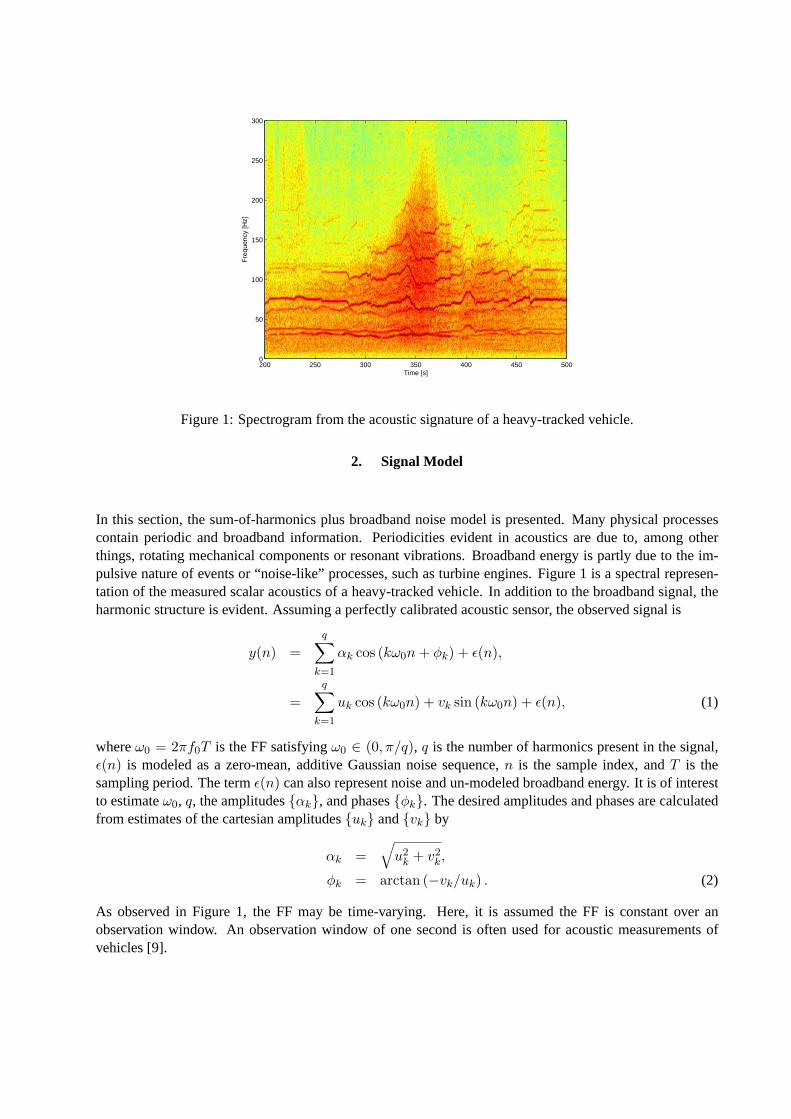
Figure 1: Spectrogram from the acoustic signature of a heavy-tracked vehicle.

2. Signal Model

In this section, the sum-of-harmonics plus broadband noise model is presented. Many physical processescontain periodic and broadband information. Periodicities evident in acoustics are due to, among otherthings, rotating mechanical components or resonant vibrations. Broadband energy is partly due to the im-pulsive nature of events or “noise-like” processes, such as turbine engines. Figure 1 is a spectral represen-tation of the measured scalar acoustics of a heavy-tracked vehicle. In addition to the broadband signal, theharmonic structure is evident. Assuming a perfectly calibrated acoustic sensor, the observed signal is

y(n) =q∑

k=1

αk cos (kω0n + φk) + ε(n),

=q∑

k=1

uk cos (kω0n) + vk sin (kω0n) + ε(n), (1)

whereω0 = 2πf0T is the FF satisfyingω0 ∈ (0, π/q), q is the number of harmonics present in the signal,ε(n) is modeled as a zero-mean, additive Gaussian noise sequence,n is the sample index, andT is thesampling period. The termε(n) can also represent noise and un-modeled broadband energy. It is of interestto estimateω0, q, the amplitudes{αk}, and phases{φk}. The desired amplitudes and phases are calculatedfrom estimates of the cartesian amplitudes{uk} and{vk} by

αk =√

u2k + v2

k,

φk = arctan (−vk/uk) . (2)

As observed in Figure 1, the FF may be time-varying. Here, it is assumed the FF is constant over anobservation window. An observation window of one second is often used for acoustic measurements ofvehicles [9].

The observed signal may also be written in matrix form. Lety be a vector of sampled sensor data for sampleindicesn = 0,. . . ,N − 1. Using Equation (1), the harmonic model can be written as

y = C(ω0)u + S(ω0)v + ε, (N × 1)= A(ω0)β + ε, (3)

where

u = [u1, . . . , uq]T , (q × 1)v = [v1, . . . , vq]T , (q × 1) (4)

are the amplitude vectors, and the elements of the(N × q) matricesC(ω) andS(ω) are given by

[C(ω)]n,k = cos (kωn + ϕk) , 0 ≤ n ≤ N − 1[S(ω)]n,k = sin (kωn + ϕk) , 1 ≤ k ≤ q (5)

wheren andk are the row and column indices, respectively, andϕk = kω(N − 1)/2. The phase term,ϕk, defines the phase at the middle of the observation window and guaranteesC(ω)TS(ω) = 0. From thesecond line in Equation (3), it follows thatA(ω) = [C(ω),S(ω)] andβ = [uT ,vT ]T . Amplitude and phasevectors are defined as

α = [α1, . . . , αq]T , (q × 1)φ = [φ1, . . . , φq]T . (q × 1) (6)

The cartesian amplitude vectorsu andv are viewed as the rectangular coordinates in the signal subspace〈A(ω0)〉 spanned by the columns ofA(ω0). The rectangular coordinates are related to their polar counter-parts by

u = α · cos(φ), (q × 1)v = −α · sin(φ), (q × 1) (7)

wherex · z is the scalar product of (m × 1) vectorsx andz, andcos(x) = [cos(x1), . . . , cos(xm)]T withsin(x) similarly defined.

The last term on the right hand side of Equation (3) is a vector of noise samples distributed asε ∼ N (0,Σ).The harmonic signal and broadband noise are considered statistically independent. The noise is modeled asa stationary autoregression. Formally, the AR noise is described as

ε(n) =1

A(z)e(n), (8)

whereA(z) is a stable, rational linear filter ande(n) is zero-mean white noise with varianceσ2AR. The filter

A(z) has the form

A(z) = 1 + a1z−1 + . . . + apz

−p, (9)

wherez−1 is the unit delay operator (e.g., z−px(n) = x(n− p)). The parameters ofA(z) are then given as

θAR = [a1, . . . , ap]T . (p× 1) (10)

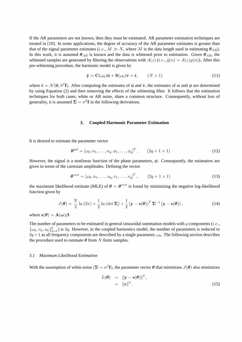
If the AR parameters are not known, then they must be estimated. AR parameter estimation techniques aretreated in [10]. In some applications, the degree of accuracy of the AR parameter estimates is greater thanthat of the signal parameter estimates (i.e., M À N , whereM is the data length used in estimatingθAR).In this work, it is assumedθAR is known and the data is whitened prior to estimation. GivenθAR, thewhitened samples are generated by filtering the observations withA(z) (i.e., y(n) = A(z)y(n)). After thispre-whitening procedure, the harmonic model is given by

y = C(ω0)u + S(ω0)v + ε, (N × 1) (11)

whereε ∼ N (0, σ2I). After computing the estimates ofu andv, the estimates ofα andφ are determinedby using Equation (2) and then removing the effects of the whitening filter. It follows that the estimationtechniques for both cases, white or AR noise, share a common structure. Consequently, without loss ofgenerality, it is assumedΣ = σ2I in the following derivations.

3. Coupled Harmonic Parameter Estimation

It is desired to estimate the parameter vector

θpol = [ω0, α1, . . . , αq, φ1, . . . , φq]T . (2q + 1× 1) (12)

However, the signal is a nonlinear function of the phase parameters,φ. Consequently, the estimators aregiven in terms of the cartesian amplitudes. Defining the vector

θrect = [ω0, u1, . . . , uq, v1, . . . , vq]T , (2q + 1× 1) (13)

the maximum likelihood estimate (MLE) ofθ = θrect is found by minimizing the negative log-likelihoodfunction given by

J(θ) =N

2ln (2π) +

12

ln (detΣ) +12

(y − s(θ))T Σ−1 (y − s(θ)) , (14)

wheres(θ) = A(ω)β.

The number of parameters to be estimated in general sinusoidal summation models withq components (i.e.,{ωk, vk, uk}q

k=1) is 3q. However, in the coupled harmonics model, the number of parameters is reduced to2q+1 as all frequency components are described by a single parameter,ω0. The following section describesthe procedure used to estimateθ from N finite samples.

3.1 Maximum Likelihood Estimation

With the assumption of white noise(Σ = σ2I), the parameter vectorθ that minimizesJ(θ) also minimizes

L(θ) = ‖y − s(θ)‖2 ,

= ‖ε‖2 . (15)

Equation (15) is the squared norm of the difference between the measurement and the signal model. Notethat the constant term due to the noise variance is ignored since it does not impact the minimization ofJ(θ). For the chosen model ofs(n), the estimation of the parameter vectorθ is a highly nonlinear process.However, the minimization of Equation (15) can be achieved by the method of least-squares (LS) ifω0 andq are assumed known. In practice, a grid search over candidateω is performed. For a candidateω and afixed q, the cartesian amplitude estimates are found by

{u(ω), v(ω)} = arg min{u,v}

‖y −C(ω)u− S(ω)v‖2 . (16)

The LS solutions to Equation (16) can be decoupled and obtained by

u =(CTC

)−1CTy,

v =(STS

)−1STy, (17)

where the dependance on the frequency has been suppressed to simplify the notation. Givenu andv, theamplitude estimates{αk} and phase estimates{φk} are found using Equation (2).

It is straightforward to show that the productATA must be block diagonal to ensure exact decoupling ofthe amplitude estimates. Diagonality is guaranteed by defining the phase of the candidate signal at thecenter of the observation window. Otherwise, the above product is approximately block diagonal for largedata lengths. As noted in [2], there is a computational benefit from decoupling the amplitude estimates.AssumingN À q, the complexity of computing the LS estimates in Equation (17) isO(2Nq2). Thecomplexity more than doubles without decoupling.

Using the LS amplitude estimates of Equation (17), the loss function for fundamental frequency estimates(FFEs) is given by

L(ω) = ‖y −Cu− Sv‖2 ,

=∥∥y −C(CTC)−1CTy − S(STS)−1STy

∥∥2,

=∥∥y −A(AA)−1ATy

∥∥2,

= yTP⊥y, (18)

whereP⊥ = I −A(ATA)−1AT = I − P projects the observation into the null space ofA. Finally, themaximum likelihood (ML) FFE is given by

ω0 = arg minω

L(ω),

= arg minω

yTP⊥y. (19)

This minimization procedure is also known as the nonlinear least-squares (NLS) method. In determiningω0, the estimator attempts to minimize (maximize) the energy in the null space (column space) ofA. Al-though there are2q + 1 free parameters, the NLS method reduces the parameter search to a1-dimensional(1-D) search. Onceω0 has been computed, the ML cartesian amplitude estimates are simply given byEquation (17).

Now, an approximation to the NLS method is considered. For large sample lengths (i.e., N → ∞) theapproximationsCTC ≈ N

2 Iq andSTS ≈ N2 Iq, whereIm is the (m × m) identity matrix, are made.

Therefore, the loss function of Equation (18) can be approximated by

L(ω) ≈∥∥∥∥y −

2N

CCTy − 2N

SSTy∥∥∥∥

2

,

=∥∥∥∥(I− 2

NAAT

)y∥∥∥∥

2

. (20)

The FFEs from the minimization of Equation (20) for finite data lengths are not ML, but are howeverasymptotically efficient in data length. Furthermore, the approximation to the ML FFE provides compu-tational savings whenq > 2. The complexity of Equation (18) isO(2Nq2), whereas the complexity ofEquation (20) isO(4Nq).

As demonstrated by [11] for complex sinusoids and [12] for real sinusoids, the NLS method still givesconsistent, although no longer ML, parameter estimates in colored Gaussian noise without the pre-whiteningstep. However, the order selection methods used here, as discussed below, require the noise be uncorrelated.Therefore, pre-whitening is a necessary step in the proposed algorithm.

3.2 Cramer-Rao Bounds

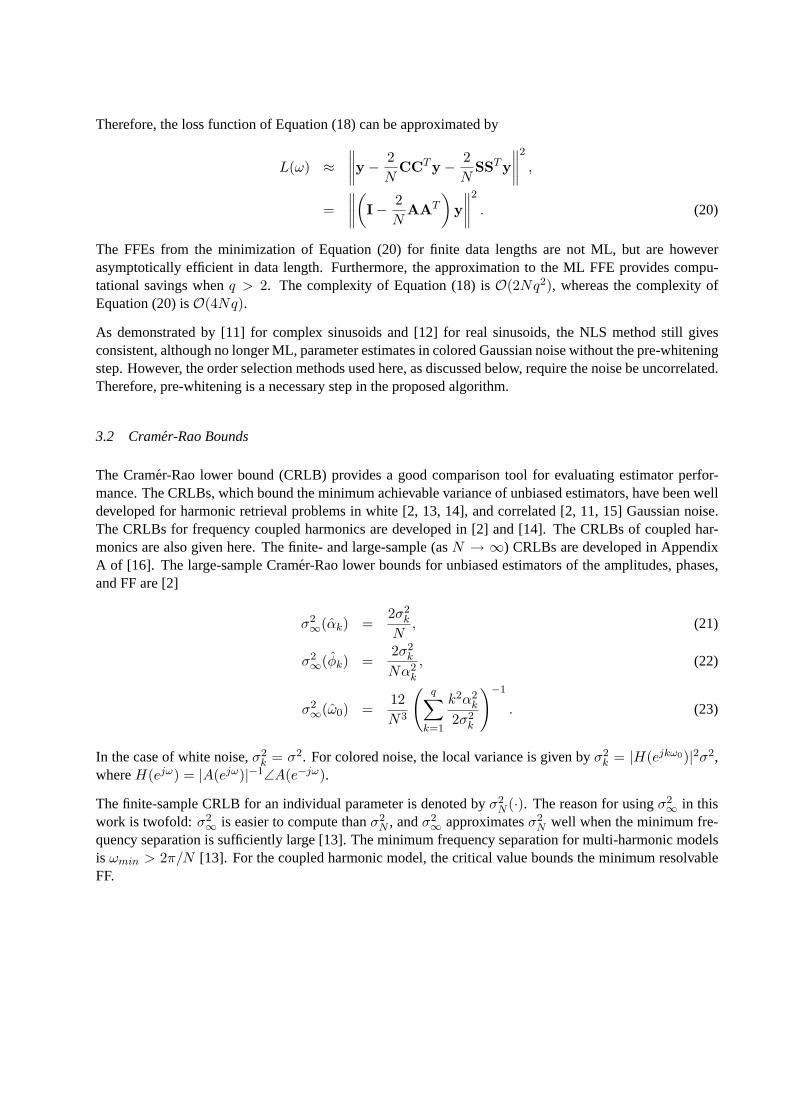
The Cramer-Rao lower bound (CRLB) provides a good comparison tool for evaluating estimator perfor-mance. The CRLBs, which bound the minimum achievable variance of unbiased estimators, have been welldeveloped for harmonic retrieval problems in white [2, 13, 14], and correlated [2, 11, 15] Gaussian noise.The CRLBs for frequency coupled harmonics are developed in [2] and [14]. The CRLBs of coupled har-monics are also given here. The finite- and large-sample (asN → ∞) CRLBs are developed in AppendixA of [16]. The large-sample Cramer-Rao lower bounds for unbiased estimators of the amplitudes, phases,and FF are [2]

σ2∞(αk) =

2σ2k

N, (21)

σ2∞(φk) =

2σ2k

Nα2k

, (22)

σ2∞(ω0) =

12N3

(q∑

k=1

k2α2k

2σ2k

)−1

. (23)

In the case of white noise,σ2k = σ2. For colored noise, the local variance is given byσ2

k = |H(ejkω0)|2σ2,whereH(ejω) = |A(ejω)|−1∠A(e−jω).

The finite-sample CRLB for an individual parameter is denoted byσ2N (·). The reason for usingσ2∞ in this

work is twofold: σ2∞ is easier to compute thanσ2N , andσ2∞ approximatesσ2

N well when the minimum fre-quency separation is sufficiently large [13]. The minimum frequency separation for multi-harmonic modelsis ωmin > 2π/N [13]. For the coupled harmonic model, the critical value bounds the minimum resolvableFF.

0.05 0.1 0.15 0.2 0.25 0.30

0.5

1

1.5

ω [radians/sample] (a)

L(ω)

[× 1

03 ]

0.05 0.1 0.15 0.2 0.25 0.30

0.5

1

1.5

L(ω)

[× 1

03 ]

ω [radians/sample] (b)

Figure 2: Loss function for a noiseless signal and the system order set to (a)r = 2 (under-set order) and(b) r = 5 (correct order) in estimating the FF. The actual number of harmonics isq = 5 with ω0 = 0.1radians/sample and uniform harmonic signal amplitudes.

3.3 Loss Function Characteristics

The frequency estimate defined in Equation (19) is derived under the assumptionq is known. If the truenumber of harmonic lines is not known, FFEs can be highly biased if the number of columns,r, in Equa-tion (5) is set incorrectly (i.e., r 6= q). Here,r is referred to as the system order. The loss function definedby Equation (18) is multi-modal. This property of the loss function gives rise to biased frequency estimateswhen the system order is incorrect. Two examples that follow demonstrate this behavior.

Figure 2 shows two plots for the loss function of the frequency estimates of a noiseless signal. The true FF isω0 = 0.1 radians/sample and the true number of harmonics isq = 5. Also, the amplitudes of the harmonicsare set to unity and the phases are random. The simulated signals are generated from a 1 second windowwith N = 512 samples. The loss function values for candidate frequencies at0.1 and0.2 radians/sampleare nearly equal when the system order is set tor = 2, as shown in Figure 2(a). In the presence of noise, theglobal minimum of the loss function may well be2ω0 for this case. As a result, Equation (18) could givehighly biased FFEs. If the number of harmonics in the signal is known, then Figure 2(b) is representative ofthe expected loss function for candidate frequencies. Here, the global minimum corresponds to the correctFF. A similar situation occurs for other amplitude models [16]. As demonstrated in [16], the global minimummay correspond toω0/2 for an over-set system order.

The frequency estimates using Equation (18), when biased, are multiples of the true FF for sufficiently highSNR and frequency resolution. Conditions for the frequency resolution are discussed below. For the coupledharmonic model, the initial estimates are given by the NLS solution for a reasonable choice ofr. Then, anaccurate estimate of the true FF can be determined by the use of order estimates.

As determined by [13], harmonics embedded in noise can be estimated very accurately given good initialestimates. This is evident in the deep, narrow troughs in Figure 2. This also suggests that a rather fine search

grid is required to ensure a candidate frequency lands in a trough of the loss function. So, it is of interest todetermine an adequate frequency resolution. In what follows is a rudimentary guide to determine a suitablefrequency search grid spacing.

To simplify the analysis, it is assumed the coupled harmonics have unit amplitudes andq is known. Dueto sampling with a finite length window, each harmonic has an associated spectrum. For a rectangularwindow, each harmonic will have asin(ωN/2)/ sin(ω/2) spectrum centered at the harmonic frequency.Consequently, each spectrum has a corresponding main beam in which most of the energy is located. Thewidth of the main beam is defined here using the beamwidth between the first nulls (BWBN). The BWBNfor the spectrum of a rectangular window is4π/N .

When the candidate FF is offset from the actual FF byδω, the spectrum of thekth candidate harmonic isshifted in frequency bykδω from that of thekth true harmonic. Whenkδω = 2π/N , thekth candidatespectrum is orthogonal to the spectrums of the true harmonic frequencies (C(ω0)TC(ω0 + 2π/kN)k = 0andS(ω0)TS(ω0 + 2π/kN)k = 0, whereC(ω)k andS(ω)k are thekth columns ofC(ω) andS(ω),respectively). Consequently, no energy from thekth candidate harmonic contributes in minimizing the NLSloss function. In addition, orthogonality for thekth harmonic also holds whenδω is an integer multiple of2π/kN . So for example, whenq is even andδω = 4π/qN , the spectrums of the middle and last candidateharmonics are orthogonal to each of those in the true signal. Incidentally, whenδω = 4π/qN , the spectralmain lobes from the last candidate and true harmonic no longer overlap. It follows that the loss functionevaluated at candidate frequencies in the vicinity of the true fundamental with increasing offset in the range2π/qN < δω < 4π/qN will take on increasingly large values. As a result, the suggested frequency searchgrid spacing is∆ω = BWBN/2q.

3.4 Comments

Dommermuth [6] proposed a loss function that averages the squared errors over possibly non-overlappingtime windows. However, time averaging may increase estimate variances because of the large sample re-quirements for the NLS method and the increased potential for model mismatches. A similar but alternatemethod could be used in sensor array applications. Instead of averagingL(ω) over data blocks, the lossfunction can be averaged over sensors. It should be noted that this alternative averaging approach assumesparameter estimation is done prior to beamforming.

4. Model Order Selection

In general, the number of significant harmonics is unknown. Therefore, it is of interest to use the modelorder information to properly choose the correct FF. Several standard order selection techniques are wellsuited to this task. These methods include Akaike’s information criterion (AIC), Rissanen’s minimum de-scription length (MDL), and maximuma posteriori probability (MAP) [17]. AIC and MDL are derivedfrom Information Theoretic Criterion (ITC), whereas MAP is derived from asymptotic Bayesian decisiontheory. Each method has a similar form with a data term and a penalty term. The penalty term accounts forthe reduced fit error when the model order is overestimated. For sinusoidal summation models, the order

selection criteria have the form [18]

qAIC = arg minr

{N lnJ(θ) + 3r

}, (24)

qMDL = arg minr

{N lnJ(θ) +

3r

2ln N

}, (25)

qMAP = arg minr

{N lnJ(θ) +

5r

2ln N

}, (26)

whereJ(θ) is the negative log-likelihood function evaluated at the ML parameter vectorθ and q is theestimate of the number of sinusoids. Each respective method is denoted by the corresponding subscript.The number of free parameters in this case is3q. However, the coupled harmonic model has2q + 1 freeparameters. The MAP criterion penalizes each unknown amplitude and phase parameter by1

2 lnN and eachunknown frequency by32 ln N [17]. As a result, the order selection criteria for the coupled harmonic modelare

qAIC = arg minr

{N ln J(θ) + 2r + 1

}= arg min

r

{N lnJ(θ) + 2r

}, (27)

qMDL = arg minr

{N ln J(θ) +

2r + 12

ln N

}= arg min

r

{N ln J(θ) + r ln N

}, (28)

qMAP = arg minr

{N ln J(θ) +

2r + 32

ln N

}= arg min

r

{N ln J(θ) + r ln N

}, (29)

whereJ(θ) is defined by Equation (14). The second equality in the three equations above are obtained byremoving terms that do not depend onr. Note that the MDL and MAP criteria are equivalent. They theydiffer from AIC by a factor of12 ln N in the second term. The second term penalizes large model orders, soin general AIC tends to give higher model orders than MDL.

The above decision rules were developed under a white Gaussian noise assumption. Another selection rule,proposed by Wang in [19], for the colored noise case has the form

qCOL = arg minr

{N lnJ(θ) +

cr

2ln N

}, (30)

wherec is a constant greater than a thresholdγ, which depends on the characteristics of the noise.

It was noted in [17] that Equation (30) can give inconsistent estimates based on the choice ofc. In addition, itwas determined in [20] that AIC produces inconsistent estimates and tends to overestimate the model order,whereas MDL yields consistent estimates for large sample records. Due to the consistency of MDL, it is thepreferred order selection method considered here. The rule proposed by Wang is not examined further, butis a possible extension of this work.

The combined detection-estimation algorithm for coupled harmonics has the form

{θ, q} = arg min{θ,r}

{N ln J(θ) + r lnN} ,

= arg min{θ,r}

{N ln L(θ) + r ln N} , (31)

where the MDL criteria represents the detection component andL(θ), given by Equation (15), representsthe estimation component. Since the estimation component can be reduced to a 1-D search it follows that

the combined algorithm can be reduced to a 2-D search. Thus, combining Equation (18) with Equation (31)the FF and order estimates are found by

{ω0, q} = arg min{ω,r}

N ln(yTP⊥y) + r lnN,

= arg min{ω,r}

h(ω, r). (32)

Then, the amplitude estimates are generated using Equation (17) with the estimatesω0 andq. Whenq = q,ω0 is the MLE. Otherwise, whenq 6= q, Equation (32) can still be used to generate statistically efficientFFEs (i.e., var(ω0) = σ2∞(ω0)), as it will be shown through simulations. In the case of colored noise,y issimply replaced byy in Equation (32).

4.1 Proposed Algorithm

It is important to estimate both the parameter set and model order together. Since the order selection methodsdepend on the parameter estimates, the order estimates may be highly biased when the FF estimates arebiased. This frequency-order dependence is evident in Figure 3. The simulated signal is composed ofq = 7harmonics withω0 = 0.1 radians/sample. The SNR, defined asρ = αT α/2σ2, of the simulated white noiseis set toρ = 3dB. Each curve in Figure 3 represents the loss function defined by Equation (32) evaluatedat a fixed frequency (preciselyω0/3, ω0/2, ω0, 2ω0, 3ω0) for a range ofr ∈ [2, min(32, rnyq)], wherernyq < bπ/ωc satisfies the Nyquist criterion. As seen in Figure 3, the global minimum corresponds to thecorrect FF and order. Notice that the minimum of the loss function for a frequency other than the correctFF does not correspond to the correct order. Also apparent in Figure 3 is that the loss function evaluated atω0 has a range ofr such that, although not the global minimum, the function is less than the minimum atcandidate frequencies at the same order.

In practice, the procedure of Equation (32) requires a fine grid search over frequency and all possible integerorders. This approach is computationally burdensome. However, it is possible to find the global minimumwith a reduced search grid. Recall the general pattern of the loss function versus frequency (no orderselection). As seen in Figure 2, deep, narrow troughs occur at the FF, sub- and super-harmonics. As notedpreviously, this suggests that these frequencies, although not necessarily the true FF, can be estimated witha high degree of accuracy. Withr properly set, an initial FF estimate, denotedωi, will likely correspond tothe true FF or multiple thereof. A reduced frequency search set can be defined using the initial frequencyestimate (e.g., ω ∈ {ωi/2, ωi, 2ωi, 3ωi}). Then, the loss function can be minimized over the new frequencyset and model order. This initialization and the combined order selection/estimation is the basis behind thealgorithms proposed in this paper. The first algorithm is detailed in Table 1. The algorithm is referred to asthe NLS-MDL method. The algorithm is basically a two stage procedure: first, generate an initial FFE, and,second, generate the order and parameter vector estimates.

It is assumed that the signals are anti-alias filtered and any DC bias is removed. Therefore, the harmonicsmust satisfykω0 ∈ (0, π) for k ∈ {1, . . . , q}. This requirement bounds above the model order correspondingto each FF. However, high orders are possible for lower fundamental frequencies. Therefore, order searchesfor lower frequencies require more computations than for higher frequencies. In general, the frequency andorder search regions would normally be confined by prior knowledge. For example, the frequency searchregion for the simulations in this work is uniformly confined tof ∈ Λf = [2, 25] Hz, which is a relaxedregion based on prior knowledge on battlefield acoustics [1]. It has also been determined that a samplingrate on the order of 0.5-1 kHz is sufficient [1, 9] for most acoustic vehicle detection and classification

5 10 15 20 25 303.4

3.5

3.6

3.7

3.8

3.9

4

4.1

4.2

h(ω

,r)

[× 1

03 ]

Order, r

ω0/3

ω0/2

ω0

2ω0

3ω0

Figure 3: Loss function for a noisy signal using MDL, evaluated at exact values ofω0/3, ω0/2, ω0, 2ω0,and3ω0, with ω0 = 0.1 radians/sample. The true number of harmonics isq = 7 with uniform amplitudesandρ = 3 dB.

applications. On the other hand, order estimates presented here are upper bounded by the criterionrub =min(rmax, rnyq), wherermax is chosen to minimize computations and as a practical limit. Alternatively,to employ lessad hoc means, methods such as those proposed by [18] could be implemented to bound theorder search region.

The initial estimates in Steps 2 and 3 are generated using likely over-set system orders. Assumingrmax

is set properly, over-setting the system order ensures that initial FFEs have minimal variance and the meancorresponds to the true FF or a sub-harmonic. Then, any large FFE bias is removed using order selection,hence the procedure in Step 5.

Table 1: Summary of the NLS-MDL Algorithm.

1. Pre-whiten the samples if the noise is correlated using the known AR model byy(n) = A(z)y(n).2. Obtain an initial estimate,ωi, of the FF using Equation (18) with a fine frequency search grid

from Λω andr set torub.3. Compute a refined initial estimate,ωi, using an optimization technique (e.g., fminbnd in MATLAB),

Equation (18), andr set torub.4. Create a new frequency search set from the refined estimate:

Λωi = {ω = αωi|α ∈ {1/b} ∪ {b}, b ∈ Z} ⊂ Λω.5. Minimize Equation (32) overΛωi and candidate orders inΛr = {2, 3, . . . , rub} to getω0 andq.6. Finally, use Equations (17) and (2) withω0 andq to get estimatesα andφ.7. Remove the effects of pre-whitening fromα andφ. If the noise is white, skip Steps 1 and 7.

A second algorithm, referred to as ANLS-MDL, utilizes the approximated NLS method of Equation (20).The ANLS-MDL algorithm substitutes Equation (20) for (18) in Step 3 of the NLS-MDL algorithm. Also,Equation (20) is combined with Equation (31), which is then substituted for Equation (32) in Step 5. Itwas determined empirically that the estimate variance of ANLS-MDL is improved by repeating Step 3 withEquation (20) andr = q after Step 5. Repeating Step 3 after Step 5 for NLS-MDL does not provide anynoticeable improvement.

5. Numerical Results

5.1 Synthetic Data Results

The following are numerical examples that demonstrate statistical properties of the combined detection-estimation algorithm. This study compares the NLS-MDL algorithm with ANLS-MDL and NLS withknown or fixed order. The algorithms are examined with simulated correlated Gaussian noise. Resultsfor simulations with white noise are presented in [16].

First, the performance of each algorithm is tested against the large-sample Cramer-Rao lower bounds ofEquations (21)-(23) on estimate variances versus SNR. Then, the algorithms are compared against theCRLBs as the true number of harmonics vary. Comparisons are made between the estimate RMSEs andthe corresponding large-sample root-CRLBs (i.e.,

√σ2∞(ω0)). The root-CRLBs will simply be referred to

as the CRLBs.

The simulation parameters common to the simulations are as follows:

• The sampling periodT is set to 1/512 s.

• The FF isω0 = 0.1 radians/sample.

• One amplitude model is examined:1/√

ω. A uniform amplitude model is also considered in [16].

• The phases are set toφk = kπ/100.

• The maximum order in the search range is set torub = min(32, bπ/ωc).• The frequency search range is set toω ∈ Λω = [π/128, 25π/256] radians/sample ([2,25] Hz) with a

frequency resolution ofπ/8N radians/sample (1/8 Hz).

• The simulation results are generated from 500 Monte-Carlo simulations.

5.1.1 Algorithm Performance versus SNR in Colored Noise

In this section, NLS-MDL and ANLS-MDL are compared with NLS with the correct order (i.e., r = q).The NLS method withr = q will simply be referred to as NLS. The CRLBs in this case are calculated usingEquations (21)-(23) with the local noise variance defined asσ2

k = |H(ejkω0)|2σ2. The following results aregenerated using pre-whitening in Step 1 of the NLS-MDL and ANLS-MDL algorithms.

0 0.1 0.2 0.3 0.4 0.5 0.6 0.7 0.8 0.9 1−150

−100

−50

0

50

Normalized Frequency (×π rad/sample)

Pha

se (

degr

ees)

0 0.1 0.2 0.3 0.4 0.5 0.6 0.7 0.8 0.9 1−20

−10

0

10

20

30

Normalized Frequency (×π rad/sample)

Mag

nitu

de (

dB)

Figure 4: Magnitude (top) and phase (bottom) response of the coloring filter,H(ejω).

The noise is generated by filtering zero-mean, unit variance Gaussian noise with a fifth order AR coloringfilter given by

H(z) ≈ 11− 2.0z−1 + 1.57z−2 − 0.28z−3 − 0.36z−4 + 0.23z−5

, (33)

and then scaled byσ = (αT α/2ρσ2AR)1/2 to achieve the desired SNR. The choice of this model is based

on measurements collected at Aberdeen Proving Grounds (APG). The lowpass filter represented by Equa-tion (33) is specific to the local environment at the time in which the measurements were recorded. However,a model needed to be adopted for these simulations. An extension of this work may include a performanceanalysis with the use of bandpass and/or highpass coloring filters. The frequency response of the coloringfilter of Equation (33) is plotted in Figure 4.

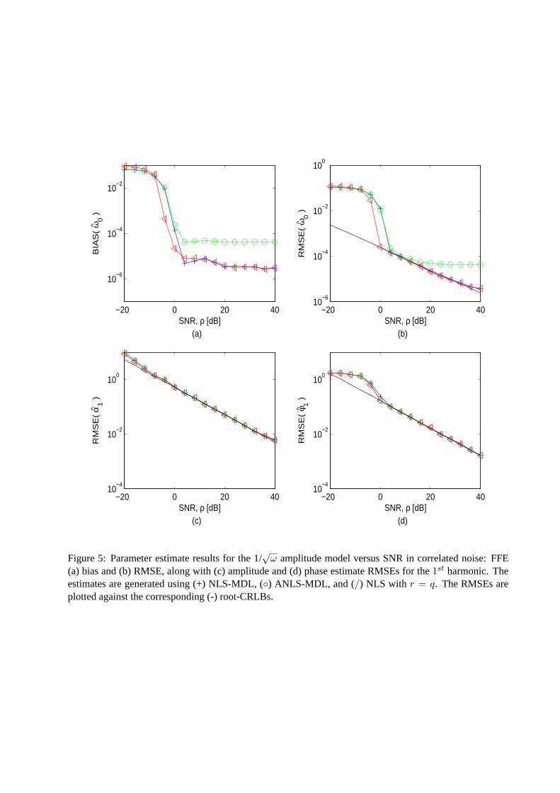
For the1/√

ω amplitude model, the absolute value of bias and the RMSE of the frequency estimates areplotted in Figures 5(a) and (b). The RMSEs of the amplitudes and phases for the first harmonic are plottedin Figures 5(c) and (d), respectively. In each figure of estimate RMSE the results are shown with thecorresponding root-CRLB.

As seen from Figure 5, the RMSEs from each algorithm correspond well with the CRLB for a large rangeof SNRs. The estimation accuracy of the NLS-MDL and ANLS-MDL algorithms degrades rapidly below 4dB SNR. The performance of the NLS algorithm does not diverge from the CRLB for decreasing SNR untilapproximately 0 dB. Note that number of harmonics of NLS is set to the correct number. It follows thatthe loss in performance of the NLS-MDL and ANLS-MDL between 0 and 4 dB SNR is mainly due to theuncertainty in the unknown number of harmonics.

The 4 dB SNR threshold for the NLS-MDL and ANLS-MDL methods is the same for a uniform amplitudemodel and is slightly higher than the threshold in the white noise case [16]. On the other hand, fewer than1% of the FFEs from NLS-MDL and ANLS-MDL constitute outlying estimates at 0 dB SNR. As shownin [16], the outlying FFEs correspond to outlying order estimates.

−20 0 20 40

10−6

10−4

10−2

SNR, ρ [dB] (a)

BIA

S(

ω0 )

−20 0 20 4010

−6

10−4

10−2

100

SNR, ρ [dB] (b)

RM

SE

( ω

0 )

−20 0 20 4010

−4

10−2

100

SNR, ρ [dB] (c)

RM

SE

( α

1 )

−20 0 20 4010

−4

10−2

100

SNR, ρ [dB] (d)

RM

SE

( φ 1

)

Figure 5: Parameter estimate results for the 1/√

ω amplitude model versus SNR in correlated noise: FFE(a) bias and (b) RMSE, along with (c) amplitude and (d) phase estimate RMSEs for the1st harmonic. Theestimates are generated using (+) NLS-MDL, (◦) ANLS-MDL, and (/) NLS with r = q. The RMSEs areplotted against the corresponding (-) root-CRLBs.

5 10 15 20 25 30−0.05

0

0.05

0.1

0.15

0.2

0.25

0.3

Harmonic Lines, q (a)

BIA

S(

ω0 )

5 10 15 20 25 30

10−5

100

Harmonic Lines, q (b)

RM

SE

( ω

0 )

Figure 6: FFE results for the1/√

ω amplitude model versus the true number of harmonics in correlatednoise: FFE (a) bias and (b) RMSE. The estimates are generated using the (+) NLS-MDL, (◦) ANLS-MDL,(/) NLS with r = 10, and (×) NLS with r = 16. The RMSEs are plotted against the (-) root-CRLB for FFEs.

The RMSEs for the higher harmonics (i.e., αk and φk, for k = {5, 10}), given in [16], are shown tobehavior similar to the RMSEs in Figures 5(c) and (d). Also, although the FFE bias evident in Figure 5(a)is insignificant compared to the true value, it is shown in [16] that the bias decreases with increasing datalength.

5.1.2 Algorithm Performance versus the Number of Harmonics in Colored Noise

Now, the performance is compared to the CRLBs as a function of the true number of harmonics in colorednoise. The number of harmonics considered isq ∈ [2, 30] in increments of 2. The orders of the NLS methodare fixed atr = 10 and 16. The data length is set toN = 256. The noise variance is adjusted as describedin Section 5.1.1 for a desired SNR ofρ = 10 dB.

The bias and RMSE of the FFEs are plotted in Figures 6(a) and (b), respectively. From Figure 6(b), it isobserved that RMSEs of the NLS-MDL and ANLS-MDL methods correspond well with the CRLB whenq ≥ 8. However, only16.8% of the FFEs from ANLS-MDL and3.4% from NLS-MDL are close toω0/4whenq = 6. Again, the outlying FFEs, which attribute to the increased RMSE, correspond to outlying orderestimates. These percentages are improved compared to the white noise case and worse than those in theuniform amplitude case [16].

The NLS methods with fixed orders only perform well over a small range ofq. The estimate variancescoincide with the CRLBs only in the ranges6 ≤ q ≤ 10 for NLS with r = 10 and10 ≤ q ≤ 16 for NLSwith r = 16. Outside these ranges, the estimates become biased toward sub- and super-harmonics. Thissuggests that the performance of the NLS method is comparable to the CRLB as long as the fixed order isin the rangeq ≤ r < 2q.

5.2 Field Measurement Data

The following example is a comparison between the STFT and parameter and order estimates using ANLS-MDL from measured data. The field data consists of noise due to the local environment and a single sourcegenerating coupled harmonics and un-modeled broadband energy. The source is a heavy-tracked battlefieldvehicle. The data was collected at APG, as part of the U.S. Army Research Laboratory’s ATR acousticdatabase, using a seven-sensor, circular microphone array.

The data was recorded atT = 1/1024 seconds/sample. The noise is assumed to be stationary and ismodeled as a fifth-order (p = 5) AR process. The AR parameters are generated using the first 10 seconds(M = 10 240 samples) of data using the least-squares method given in [10]. The data length for the STFTis N = 1024, whereas the data length for ANLS-MDL isN = 512. Non-overlapping rectangular windowsare used for both the STFT and ANLS-MDL. The frequency and order search regions are the same as thoseitemized in Section 5.1. In contrast, the minimum allowable order is set tormin = 0. The frequency lossfunction is averaged using data from all seven sensors, as briefly discussed in Section 3.4. Consequently,amplitude and phase estimates are generated from each sensor’s data. However, only the results from Sensor1 are presented.

The STFT of the raw data from Sensor 1 is represented by a spectrogram in Figure 7(a). In Figure 7(b),the harmonic frequency estimates from each half-second data block are plotted along the vertical axis. Thehorizontal axis represents the progression of time. The relative amplitudes of the spectral data are scaled indecibels.

Up to approximately 200 seconds, ANLS-MDL estimates, for the most part, that there is no harmonic signal.Beyond 200 seconds, it appears the ANLS-MDL frequency and amplitude estimates are well-related to themeasured harmonic source. The range of the source from the sensor array at 200 seconds is approximately1 km. The closest point of approach (CPA) of the source occurs at 380 seconds. The estimates from ANLS-MDL also appear to improve up to and beyond the CPA.

The parameters are generated using independent half-second blocks of data. Although the parameter esti-mates are independent from block to block, there is an obvious continuity in the low to mid-range harmonicsover time, as seen in Figure 7(b).

Using a CLEAN type approach, the signal estimates are subtracted from the whitened data, resulting in theresidual signal. The spectrogram for the residual data is shown in Figure 8. As seen in the figure, most ofthe remaining energy corresponds to un-modeled broadband energy and a pair of possibly coupled harmoniclines.

Time [s] (a)

Fre

quency

[H

z]

0 100 200 300 400 5000

50

100

150

200

250

300

0 100 200 300 400 5000

50

100

150

200

250

300

Time [s] (b)

Fre

quency

[H

z]

Figure 7: Spectrogram (a) and harmonic line estimates (b) of the acoustic signature from a single heavy-tracked vehicle.

Time [s]

Fre

qu

en

cy [

Hz]

0 100 200 300 400 5000

50

100

150

200

250

300

Figure 8: Spectrogram of the residual whitened signal.

6. Conclusions

Two algorithms have been introduced which combine parameter estimation and order selection for coupledharmonic signals in Gaussian noise. These methods and the standard NLS method with a fixed order wereevaluated in numeric simulations. The NLS method withr = q corresponds to the maximum likelihoodestimator. However, NLS with order selection (i.e., NLS-MDL) exhibits only slight loss in performancecompared to the MLEs, and at the expense of computational complexity. The loss in performance is ac-credited to the uncertainty in the true number of harmonics. However, the performance differences quicklydiminish with increasing SNR and data length. Additionally, the ANLS-MDL method offers similar perfor-mance to NLS-MDL with fewer computations.

Each algorithm has an associated SNR and sample length thresholds (data length thresholds are shownin [16] to beN > 256 for ρ = 0 dB). For sufficient SNR and data length, the NLS method providesstatistically efficient estimates when the number of harmonics is known. However, when the number ofharmonics is not known, but the system order is fixed, the NLS method still provides statistically efficientestimates providedq ≤ r < 2q. Also, when the number of harmonics is not known, the proposed algorithmsprovide statistically efficient estimates for sufficient SNR, data length, and harmonic lines. In battlefieldacoustics, the number of harmonics is generally not known and the number can vary, as seen in Figures 1and 7.

In conclusion, the proposed algorithms are efficient methods that can be used to extract features, such asthe FF or phase parameters, of single sources generating coupled harmonics. These features are useful intarget classification [1] or in DOA estimation. In addition, these algorithms can also be used to initializeand periodically update algorithms designed to track time-varying parameters, which generally require priorknowledge of the number of parameters to track. In the case of multiple sources, these algorithms can becombined with beamforming to temporally and spatially separate targets.

Acknowledgement

Any opinions, findings, and conclusions or recommendations expressed in this publication are those ofthe authors and do not necessarily reflect the views of the U.S. Army Research Laboratory or the U.S.Government.

References

[1] M. Wellman, N. Srour, and D. Hillis, “Acoustic Feature Extraction for a Neural Network Classifier,”ARL Tech. Report, vol. ARL-TR-1166, pp. 11–12, Jan 1997.

[2] D. Lake, “Efficient Maximum Likelihood Estimation of Multiple and Coupled Harmonics,”ARL Tech.Report, vol. ARL-TR-2014, Dec 2000.

[3] A. Nehorai and B. Porat, “Adaptive Comb Filtering for Harmonic Signal Enhancement,”IEEE Trans.Acous., Spch., and Sig. Proc., vol. 34, pp. 378–392, Oct 1986.

[4] B. James, B. D. O. Anderson, and R. Williamson, “Conditional Mean and Maximum Likelihood Ap-proaches to Multiharmonic Frequency Estimation,”IEEE Trans. Sig. Proc., vol. 42, pp. 1366–1375,Jun 1994.

[5] A. Ferrari, G. Alengrin, and C. Theys, “Estimation of the Fundamental Frequency of a Noisy Sum ofCisoids with Harmonic Related Frequencies,” inIEEE Int. Conf. Acous., Spch., and Sig. Proc., vol. 5,pp. 515–520, 1992.

[6] F. Dommermuth, “Estimation of Fundamental Frequencies,”IEE Radar and Sig. Proc., vol. 140,pp. 162–170, Jun 1993.

[7] S. Kay and V. Nagesha, “Extraction of Periodic Signals in Colored Noise,” inIEEE Int. Conf. Acous.,Spch., and Sig. Proc., vol. 5, pp. 281–284, 1992.

[8] J. Rissanen, “Modelling by the Shortest Data Description,”Automatica, vol. 14, pp. 465–471, 1978.

[9] T. Pham and B. Sadler, “Wideband Acoustic Array Processing to Detect and Track Ground Vehicles,”in 130th meeting of the Acoustical Society of America, Nov 1995.

[10] P. Stoica and R. Moses,Introduction to Spectral Analysis. Upper Saddle River, NJ: Prentice Hall,1997.

[11] P. Stoica, A. Jakobsson, and J. Li, “Cisoid Parameter Estimation in the Colored Noise Case: Asymp-totic Cramer-Rao Bound, Maximum Likelihood, and Nonlinear Least-Squares,”IEEE Trans. Sig.Proc., vol. 45, Aug 1997.

[12] P. Stoica and A. Nehorai, “Statistical Analysis of Two Non-Linear Least-Squares Estimators of SineWaves Parameters in the Colored Noise Case,” inIEEE Int. Conf. Acous., Spch., and Sig. Proc., vol. 4,pp. 2408–2411, 1988.

[13] P. Stoica, R. Moses, B. Friedlander, and T. Soderstrom, “Maximum Likelihood Estimation of theParameters of Multiple Sinusoids from Noisy Measurements,”IEEE Trans. Acous., Spch., and Sig.Proc., vol. 37, pp. 378–392, Mar 1989.

[14] A. Swami and M. Ghogho, “Cramer-Rao Bounds for Coupled Harmonics in Noise,” vol. 1, pp. 483–487, Nov 1997.

[15] M. Ghogho and A. Swami, “Lower Bounds on the Estimation of Harmonics in Colored Noise,” vol. 1,pp. 478–482, Nov 1997.

[16] G. Whipps, “Coupled harmonics: Estimation and detection,” Master’s thesis, The Ohio State Univer-sity, 2003.

[17] P. Djuric, “A Model Selection Rule for Sinusoids in White Gaussian Noise,”IEEE Trans. Sig. Proc.,vol. 44, pp. 1744–1751, Jul 1996.

[18] A. Sabharwal, C. Ying, L. Potter, and R. Moses, “Model Order Selection for Summation Models,”13th

Asilomar Conf. Sig., Sys., and Comp., vol. 2, pp. 1240–1244, Nov 1996.

[19] X. Wang, “An AIC Type Estimator for the Number of Cosinusoids,”Journal of Time Series Analysis,vol. 14, no. 4, pp. 433–440, 1993.

[20] M. Wax and T. Kailath, “Detection of Signals by Information Theoretic Criteria,”IEEE Trans. Sig.Proc., vol. 33, pp. 387–392, Apr 1985.