Astronomy & Astrophysics manuscript no. main c©ESO 2019August 1, 2019

Planetary system around the nearby M dwarf GJ 357 including atransiting, hot, Earth-sized planet optimal for atmospheric

characterization ?

R. Luque1,2, E. Pallé1,2, D. Kossakowski3, S. Dreizler4, J. Kemmer5, N. Espinoza3, J. Burt6,40, G. Anglada-Escudé7,8,V. J. S. Béjar1,2, J. A. Caballero9, K. A. Collins10, K. I. Collins11, M. Cortés-Contreras9, E. Díez-Alonso12,13, F. Feng14,A. Hatzes15, C. Hellier16, T. Henning3, S. V. Jeffers4, L. Kaltenegger17, M. Kürster3, J. Madden17, K. Molaverdikhani3,

D. Montes12, N. Narita1,18,19,20, G. Nowak1,2, A. Ofir21, M. Oshagh4, H. Parviainen1,2, A. Quirrenbach5, S. Reffert5,A. Reiners4, C. Rodríguez-López8, M. Schlecker3, S. Stock5, T. Trifonov3, J. N. Winn22, M. R. Zapatero Osorio23,

M. Zechmeister4, P. J. Amado8, D. R. Anderson16, N. E. Batalha24, F. F. Bauer8, P. Bluhm5, C. J. Burke6, R. P. Butler14,D. A. Caldwell25,26, G. Chen27, J. D. Crane28, D. Dragomir6,41, C. D. Dressing29, S. Dynes6, J. M. Jenkins26,

A. Kaminski5, H. Klahr3, T. Kotani18,20, M. Lafarga30,31, D. W. Latham10, P. Lewin32, S. McDermott33,P. Montañés-Rodríguez1,2, J. C. Morales30,31, F. Murgas1,2, E. Nagel34, S. Pedraz35, I. Ribas30,31, G. R. Ricker6,

P. Rowden36, S. Seager6,37,38, S. A. Shectman28, M. Tamura18,20,39, J. Teske28,41, J. D. Twicken25,26, R. Vanderspeck6,S. X. Wang14, and B. Wohler25,26

(Affiliations can be found after the references)

Received 29 April 2019 / Accepted 27 June 2019

ABSTRACT

We report the detection of a transiting Earth-size planet around GJ 357, a nearby M2.5 V star, using data from the Transiting Exoplanet SurveySatellite (TESS). GJ 357 b (TOI-562.01) is a transiting, hot, Earth-sized planet (Teq = 525 ± 11 K) with a radius of Rb = 1.217 ± 0.084 R⊕ andan orbital period of Pb = 3.93 d. Precise stellar radial velocities from CARMENES and PFS, as well as archival data from HIRES, UVES, andHARPS also display a 3.93-day periodicity, confirming the planetary nature and leading to a planetary mass of Mb = 1.84 ± 0.31 M⊕. In additionto the radial velocity signal for GJ 357 b, more periodicities are present in the data indicating the presence of two further planets in the system:GJ 357 c, with a minimum mass of Mc = 3.40 ± 0.46 M⊕ in a 9.12 d orbit, and GJ 357 d, with a minimum mass of Md = 6.1 ± 1.0 M⊕ in a 55.7 dorbit inside the habitable zone. The host is relatively inactive and exhibits a photometric rotation period of Prot = 78 ± 2 d. GJ 357 b is to datethe second closest transiting planet to the Sun, making it a prime target for further investigations such as transmission spectroscopy. Therefore,GJ 357 b represents one of the best terrestrial planets suitable for atmospheric characterization with the upcoming JWST and ground-based ELTs.

Key words. planetary systems – techniques: photometric – techniques: radial velocities – stars: individual: GJ 357 – stars: late-type

1. Introduction

To date nearly 200 exoplanets have been discovered orbiting ap-proximately 100 M dwarfs in the solar neighborhood (e.g., Bon-fils et al. 2013; Rowe et al. 2014; Trifonov et al. 2018; Ribaset al. 2018). Some of these orbit near to or in the habitable zone(e.g., Udry et al. 2007; Anglada-Escudé et al. 2013, 2016; Tuomi& Anglada-Escudé 2013; Dittmann et al. 2017; Reiners et al.2018). However, only 11 M dwarf planet systems have been de-tected with both the transit as well as the radial velocity (RV)method, which allows us to derive their density from their mea-sured radius and mass, informing us about its bulk properties.When transit timing variation (TTV) mass measurements are in-cluded, TRAPPIST-1 (2MUCD 12171, Gillon et al. 2017) rep-resents the 12th M dwarf planet system with mass and radiusmeasurements.

Only six of the abovementioned eleven systems contain plan-ets with masses below 10 M⊕: LHS 1140 b and c (GJ 3053,Dittmann et al. 2017; Ment et al. 2019), K2-3 b and c? RV data are only available in electronic form at the CDS via anony-

mous ftp to cdsarc.u-strasbg.fr (130.79.128.5) or via http://cdsweb.u-strasbg.fr/cgi-bin/qcat?J/A+A/

(PM J11293–0127, Almenara et al. 2015; Sinukoff et al. 2016),K2-18 b (PM J11302+0735, Cloutier et al. 2017; Sarkis et al.2018), GJ 1214 b (LHS 3275 b, Harpsøe et al. 2013), GJ 1132(Berta-Thompson et al. 2015; Bonfils et al. 2018), and b–g planets of TRAPPIST-1 (Gillon et al. 2016, 2017). How-ever, only three planets with masses similar to Earth orbitM dwarfs of moderate brightness (J = 9.2–9.8 mag): GJ 1132 b(1.66 ± 0.23 M⊕), LHS 1140 c (1.81 ± 0.39 M⊕), and K2-18 b(2.1+2.1

−1.3 M⊕). Systems hosting small terrestrial exoplanets orbit-ing bright stars are ideal not only from the perspective of precisemass measurements with ground-based instruments, but also forfurther orbital (e.g., obliquity determination) and atmosphericcharacterization using current and future observatories (see, e.g.,Batalha et al. 2018).

The Transiting Exoplanet Survey Satellite (TESS, Rickeret al. 2015) mission is an observatory that was launched to findsmall planets transiting small, bright stars. Indeed, since the startof scientific operations in July 2018, TESS has already uncov-ered over 600 new planet candidates, and is quickly increasingthe sample of known Earths and super-Earths around small M-type stars (Vanderspek et al. 2019; Günther et al. 2019; Kostovet al. 2019). In this paper, we present the discovery of three small

Article number, page 1 of 20

arX

iv:1

904.

1281

8v3

[as

tro-

ph.E

P] 3

0 Ju

l 201

9

A&A proofs: manuscript no. main

planets around a bright M dwarf, one of which, GJ 357 b, isan Earth-sized transiting exoplanet discovered using photometryfrom the TESS mission. To date, GJ 357 b is the second nearest(d = 9.44 pc) transiting planet to the Sun after HD 219134 b(Motalebi et al. 2015, d = 6.53 pc), and the closest aroundan M dwarf. Besides, it is amenable to future detailed atmo-spheric characterization, opening the door to new studies foratmospheric characterization of Earth-like planet atmospheres(Pallé et al. 2009).

The paper is structured as follows. Section 2 presents theTESS photometry used for the discovery of GJ 357 b. Section 3presents ground-based observations of the star including seeing-limited photometric monitoring, high-resolution imaging, andprecise RVs. Section 4 presents a detailed analysis of the stellarproperties of GJ 357. Section 5 presents an analysis of the avail-able data in order to constrain the planetary properties of the sys-tem, including precise mass constraints on GJ 357 b along witha detection and characterization of two additional planets in thesystem, GJ 357 c and GJ 357 d. Section 6 presents a discussionof our results and, finally, Sect. 7 presents our conclusions.

2. TESS photometry

Planet GJ 357 (TIC 413248763) was observed by TESS in 2-min short-cadence integrations in Sector 8 (Camera #2, CCD#3) from February 2, 2019 until February 27, 2019 (see Fig. 1),and will not be observed again during the primary mission. AtBJD = 2458531.74, an interruption in communications betweenthe instrument and spacecraft occurred, resulting in an instru-ment turn-off until BJD = 2458535.00. Together with the satel-lite repointing for data downlink between BJD = 2458529.06and BJD = 2458530.44, a gap of approximately 6 d is present inthe photometry. In our analysis, the datapoints between BJD =2458530.44 and BJD = 2458531.74 were masked out.

2.1. Transit searches

TESS objects of interest (TOIs) are announced regularly via theTESS data alerts public website1. TOI-562.01 was announced onApril 13, 2019 and its corresponding light curve produced bythe Science Processing Operations Center (SPOC; Jenkins et al.2016) at the NASA Ames Research Center was uploaded to theMikulski Archive for Space Telescopes (MAST)2 on April 17,2019. SPOC provided for this target simple aperture photometry(SAP) and systematics-corrected photometry, a procedure con-sisting of an adaptation of the Kepler Presearch Data Condition-ing algorithm (PDC, Smith et al. 2012; Stumpe et al. 2012, 2014)to TESS. The light curves generated by both methods are shownin Fig. 1. We use the latter one (PDC-corrected SAP, Fig. 1 bot-tom panel) for the remainder of this work.

A signal with a period of 3.93 d and a transit depth of1164±66 ppm, corresponding to a planet radius of approximately1.3 ± 0.3 R⊕ was detected in the TESS photometry. The Earth-sized planet candidate passed all the tests from the Alerts DataValidation Report3 (DVR; Twicken et al. 2018; Li et al. 2019),for example, even-odd transits comparison, eclipsing binary dis-crimination tests, ghost diagnostic tests to help rule out scatteredlight, or background eclipsing binaries, among others. The re-port indicates that the dimming events are associated with signif-

1 https://tess.mit.edu/alerts/2 https://mast.stsci.edu3 The complete DVR of TOI-562.01 can be downloaded from https://tev.mit.edu/vet/spoc-s08-b01/413248763/dl/pdf/.

icant image motion, which is usually indicative of a backgroundeclipsing binary. However, in this case, the reported informationis meaningless because the star is saturated. On the other hand,the transit source is coincident with the core of the stellar pointspread function (PSF), so the transit events happen on the targetand not, for example, on a nearby bright star.

We also performed an independent analysis of the TESS lightcurve in order to confirm the DVR analysis and search for addi-tional transit signals. An iterative approach was employed: ineach iteration the same raw data were detrended and outliers-rejected, a signal was identified and then modeled, and thatmodel was temporarily divided-out during the detrending of thenext iteration to produce a succession of improving models —until the χ2 converges. The raw photometry was detrended byfitting a truncated Fourier series, starting from the natural periodof twice the data span, and all of its harmonics, down to some"protected" time span to make sure the filter does not modify theshape of the transit itself. We used a protected time span of 0.5 d,and this series was iteratively fitted with 4σ rejection. Finally,OptimalBLS (Ofir 2014) is used to identify the transit signal,which is then modeled using the Mandel & Agol (2002) modeland the differential evolution Markov Chain Monte Carlo algo-rithm (ter Braak & Vrugt 2008). The final model has χ2

ν = 1.017and the resultant transit parameters are consistent with the TESSDVR. We also checked for odd-even differences between thetransits, additional transit signals, and parabolic TTVs (Ofir et al.2018) – all with null results.

2.2. Limits on photometric contamination

Given the large TESS pixel size of 21′′, it is essentialto verify that no visually close-by targets are present thatcould affect the depth of the transit. There are two brightobjects within one TESS pixel of GJ 357: (i) Gaia DR25664813824769090944 at 15.19′′ and GRP = 15.57 mag; and(ii) Gaia DR2 5664814202726212224 at 18.31′′ and GRP =15.50 mag. However, they are much fainter than GJ 357 (TOI-562, Gaia DR2 5664814198431308288, GRP = 8.79 mag) andtheir angular separations actually increased between the epochsof observation of Gaia (J2015.5) and TESS (J2019.1–J2019.2)due to the high proper motion of this star.

These two sources are by far the brightest ones apart fromour target in the digitizations of red photographic plates taken in1984 and 1996 with the UK Schmidt telescope. The Gaia GRP -band (630–1050 nm) and the TESS band (600–1000 nm) are verymuch alike, allowing us to estimate the dilution factor for TESSusing Eq. 2 in Espinoza et al. (2018) to be DTESS = 0.996, whichis consistent with 1.00, therefore compatible with no flux con-tamination.

3. Ground-based observations

3.1. Transit follow-up

We acquired ground-based time-series follow-up photometry ofa full transit of TOI-562.01 on UTC April 26, 2019 from aLas Cumbres Observatory (LCO) 1.0 m telescope (Brown et al.2013) at Cerro Tololo Inter-American Observatory (CTIO) aspart of the TESS follow-up program (TFOP) SG1 Group. Weused the TESS Transit Finder, which is a customized ver-sion of the Tapir software package (Jensen 2013), to schedulephotometric time-series follow-up observations. The 4096×4096LCO SINISTRO camera has an image scale of 0′′.389 pix−1 re-sulting in a 26′ × 26′ field of view. The 227 min observation in

Article number, page 2 of 20

R. Luque et al.: Planetary system around GJ 357

39000

39500

40000

40500

41000

Flux

(ADU

)

Simple Aperture Photometry (SAP)

8520 8525 8530 8535 8540BJD - 2450000 (d)

44800

44900

45000

45100

45200

45300

Flux

(ADU

)

PDC-corrected SAP

Fig. 1. TESS light curves of GJ 357 provided by SPOC. Top panel: Simple aperture photometry. Bottom panel: PDC-corrected photometry. Transitsof the planet candidate TOI-562.01 are marked in red.

zs band used 30 s exposure times which, in combination withthe 26 s readout time, resulted in 244 images. The images werecalibrated by the standard LCO BANZAI pipeline and the pho-tometric data were extracted using the AstroImageJ softwarepackage (Collins et al. 2017). The target star light curve showsa clear transit detection in a 7.78′′ radius aperture (see middleright panel of Fig. 5). The full width half maximum (FWHM)of the target and nearby stars is ∼ 4′′, so the follow-up apertureis only marginally contaminated by neighboring faint Gaia DR2stars. The transit signal can be reliably detected with aperturesthat have a radius as small as 4.28′′, after which systematic ef-fects start to dominate the light curve. We note that the detectionof an ∼ 1200 ppm transit with a 1 m ground-based telescope ina single transit is remarkable. A similar performance has beenachieved only with the 1.2 m Euler-Swiss telescope combiningtwo transits of HD 106315 c (Lendl et al. 2017), and highlightsthe importance of ground-based facilities to maintain and re-fine ephemeris of TESS planet candidates even in the Earth-sizedregime.

3.2. Seeing-limited photometric monitoring

We made a compilation of photometric series obtainedby long-time baseline, automated surveys exactly as inDíez Alonso et al. (2019). In particular we retrieved data fromthe following public surveys: All-Sky Automated Survey(ASAS; Pojmanski 2002), Northern Sky Variability Survey(NSVS; Wozniak et al. 2004), and All-Sky Automated Sur-vey for Supernovae (ASAS-SN; Kochanek et al. 2017). Thetelescope location, instrument configurations, and photometricbands of each public survey were summarized by Díez Alonsoet al. (2019). We did not find GJ 357 data in other public cat-alogs, such as The MEarth Project (Charbonneau et al. 2008),the Catalina surveys (Drake et al. 2014), or the Hungarian Auto-mated Telescope Network (Bakos et al. 2004).

WASP-South, the southern station of the Wide Angle Searchfor Planets (Pollacco et al. 2006), is an array of eight camerasusing 200-mm f/1.8 lenses backed by 2048 × 2048 CCDs, eachcamera covering 7.8◦ × 7.8◦. It rasters a set of different point-

ings with a typical 10-min cadence. WASP-South observed fieldscontaining GJ 357 every year from 2007 to 2012, obtaining dataover a span of typically 120 d each season, acquiring a total of48 000 photometric observations.

3.3. High-resolution imaging

FastCam Although we discuss in Sect. 2.2 that there are no vi-sually close companions that could affect the depth of the transitof GJ 357, we obtained high-resolution observations at differentepochs to exclude the possibility of a physically-bound eclips-ing binary that may produce the transits detected in the TESSlight curve. First, we observed GJ 357 with the FastCam instru-ment (Oscoz et al. 2008) mounted on the 1.5 m Telescopio Car-los Sánchez at the Teide Observatory on January 14, 2013. Theseobservations were part of our high-resolution imaging campaignof M dwarfs to characterize stellar multiplicity and select themost appropriate targets for the CARMENES survey (Cortés-Contreras et al. 2017). FastCam is a lucky imaging camera witha high readout speed, employing the subelectron noise L3CCDAndor 512×512 detector, which provides a pixel size of 0.0425′′and a field of view of 21.2′′ × 21.2′′. We obtained ten blocks ofa thousand individual frames with 50 ms exposure time in the Iband. Data were bias subtracted, aligned, and combined usingthe brightest pixel as a reference as described in Labadie et al.(2010) and Jódar et al. (2013). We selected the best 10 % of theframes to produce the final image and determined that there areno background contaminating sources with δ I < 3 mag down to0.5′′ and with δ I < 6 mag down to 3.0′′ and up to 8.5′′ (given bythe detector size).

IRD We also observed GJ 357 with the InfraRed Doppler (IRD,Kotani et al. 2018) instrument on the Subaru 8.2 m telescope onApril 18, 2019. IRD is a fibre-fed instrument through a fibre in-jection module behind an adaptive optics (AO) system (AO188,Hayano et al. 2010). A fibre injection module camera (FIMC)monitors images around targets to enable fibre injection of stel-lar light and guiding, and can take AO-corrected images of ob-

Article number, page 3 of 20

A&A proofs: manuscript no. main

Fig. 2. Adaptive-optics-corrected image taken with the fiber injectionmodule camera of IRD mounted on the Subaru 8.2 m telescope on April18, 2019. The field of view is 13.4′′×13.4′′ (200×200 pix). Color codingis assigned in logarithmic scale. North is 116 deg turned clockwise fromthe upper direction.

serving targets. The FIMC employs a CCD with pixel scale of0.067′′ per pixel and observes in 970–1050 nm. Figure 2 is theFIMC image of GJ 357. The image shows a 200 × 200 pixelregion around GJ 357, revealing no nearby point source.

We note that GJ 357 is a high proper motion star with 0.139′′per year in RA and -0.990′′ per year in DEC based on the GaiaData Release 2 (DR2) data (Gaia Collaboration et al. 2018). Itmeans that the star was about 0.8′′ to the west and about 6′′ to thenorth at the time of the FastCam observation. The FastCam andIRD FIMC non-detection of any nearby companion excludes anybackground object at the original position of the FastCam ob-servation. We exclude any false positive scenario and concludethere is no flux contamination from visually close-by targets inthe GJ 357 transit data, and we fix the dilution factor for TESSto one in all of our model fits.

3.4. Precise radial velocities

3.4.1. HIRES

The high-resolution spectrograph HIRES (Vogt et al. 1994)mounted on the 10-m Keck-I telescope has been extensively usedto search for exoplanets around bright dwarf stars using the RVtechnique (e.g., Vogt et al. 2000; Cumming et al. 2008). As partof this effort, Butler et al. (2017) published 64 480 observationsof a sample of 1699 stars collected with HIRES between 1996and 2014. These data have been recently reanalyzed by Tal-Oret al. (2019) using a sample of RV-quiet stars (i.e., whose RVscatter is < 10 m s−1), who found small, but significant system-atic effects in the RVs: a discontinuous jump caused by majormodifications of the instrument in August 2004, a long-term

drift, and a small intra-night drift. We use a total of 36 measure-ments for GJ 357 taken between January 26, 1998 and Febru-ary 20, 2013. The RVs show a median internal uncertainty of2.4 m s−1 and a rms of 4.0 m s−1 around the mean value.

3.4.2. UVES

Zechmeister et al. (2009) published 70 RV measurements ofGJ 357 taken between November 15, 2000 and March 25, 2007as part of the M dwarf planet search for terrestrial planets in thehabitable zone with UVES at the ESO Very Large Telescope.RVs were obtained with the AUSTRAL code (Endl et al. 2000) andcombined into nightly averages following Kürster et al. (2003).The 30 nightly binned RVs show a median internal uncertaintyof 2.5 m s−1 and a rms of 5.3 m s−1 around the mean value.

3.4.3. HARPS

The High Accuracy Radial velocity Planet Searcher (HARPS,Mayor et al. 2003) is an ultra-precise Échelle spectrograph inthe optical regime installed at the ESO 3.6 m telescope at LaSilla Observatory in Chile, with a sub-m s−1 precision. We re-trieved 53 high-resolution spectra from the ESO public archivecollected between December 13, 2003 and February 13, 2013.We extracted the FWHM and bisector span (BIS) of the cross-correlation function from the FITS headers as computed by theDRS ESO HARPS pipeline (Lovis & Pepe 2007), but to ob-tain the RVs we used SERVAL (Zechmeister et al. 2018), basedon least-squares fitting with a high signal-to-noise (S/N) tem-plate created by co-adding all available spectra of the star. TheRVs have a median internal uncertainty of 1 m s−1 and a rms of3.3 m s−1 around the mean value.

3.4.4. PFS

The Planet Finder Spectrograph (Crane et al. 2010) is an iodine-cell, high-precision RV instrument mounted on the 6.5 m Mag-ellan II telescope at Las Campanas Observatory in Chile. RVsare measured by placing a cell of gaseous I2 in the convergingbeam of the telescope. This imprints the 5000-6200 Å region ofincoming stellar spectra with a dense forest of I2 lines that actas a wavelength calibrator, and provide a proxy for the pointspread function (PSF) of the instrument. GJ 357 was observeda total of nine times as part of the long-term Magellan PlanetSearch Program between March 2016 and January 2019. AfterTESS’ identification of transits in GJ 357, the star was then ob-served at higher precision during the April and May 2019 runs,which added an additional seven RVs to the dataset. The iodinedata prior to February 2018 (PFSpre) were taken through a 0.5"slit resulting in R ∼ 80, 000, and those after (PFSpost) weretaken through a 0.3" slit, resulting in R ∼ 130, 000. A differ-ent offset must be accounted for the RVs taken before and afterthis intervention. All PFS data are reduced with a custom IDLpipeline that flat fields, removes cosmic rays, and subtracts scat-tered light. Additional details about the iodine-cell RV extrac-tion method can be found in Butler et al. (1996). The RVs havea median internal uncertainty of 1.3 (0.7) m s−1 and an rms of3.1 (2.3) m s−1 around the mean value for PFSpre (PFSpost).

3.4.5. CARMENES

The star GJ 357 (Karmn J09360-216) is one of the 342 starsmonitored in the CARMENES Guaranteed Time Observation

Article number, page 4 of 20

R. Luque et al.: Planetary system around GJ 357

Table 1. Stellar parameters of GJ 357.

Parameter Value ReferenceName and identifiers

Name L 678-39 Luyten (1942)GJ 357 Gliese (1957)Karmn J09360-216 AF15TOI 562 TESS AlertsTIC 413248763 Stassun et al. (2018)

Coordinates and spectral typeα 09:36:01.64 Gaia DR2δ –21:39:38.9 Gaia DR2SpT M2.5 V Hawley et al. (1996)

MagnitudesB [mag] 12.52 ± 0.02 UCAC4V [mag] 10.92 ± 0.03 UCAC4g [mag] 11.70 ± 0.02 UCAC4G [mag] 9.8804 ± 0.0014 Gaia DR2r [mag] 10.34 ± 0.09 UCAC4i [mag] 9.35 ± 0.27 UCAC4J [mag] 7.337 ± 0.034 2MASSH [mag] 6.740 ± 0.033 2MASSKs [mag] 6.475 ± 0.017 2MASS

Parallax and kinematicsπ [mas] 105.88 ± 0.06 Gaia DR2d [pc] 9.444 ± 0.005 Gaia DR2µα cos δ [mas yr−1] +138.694 ± 0.100 Gaia DR2µδ [mas yr−1] −990.311 ± 0.083 Gaia DR2Vr [km s−1] -34.70±0.50 This workU [km s−1] 41.11±0.13 This workV [km s−1] 11.37±0.45 This workW [km s−1] -37.25±0.19 This work

Photospheric parametersTeff [K] 3505 ± 51 Schweitzer et al. (2019)log g 4.94 ± 0.07 Schweitzer et al. (2019)[Fe/H] −0.12 ± 0.16 Schweitzer et al. (2019)v sin i? [km s−1] < 2.0 Reiners et al. (2018)

Physical parametersM [M�] 0.342 ± 0.011 Schweitzer et al. (2019)R [R�] 0.337 ± 0.015 Schweitzer et al. (2019)L [10−4 L�] 159.1 ± 3.6 Schweitzer et al. (2019)

References. AF15: Alonso-Floriano et al. (2015); Gaia DR2: GaiaCollaboration et al. (2018); UCAC4: Zacharias et al. (2013); 2MASS:Skrutskie et al. (2006).

program to search for exoplanets around M dwarfs, which beganin January 2016 (Reiners et al. 2018). The CARMENES instru-ment is mounted at the 3.5 m telescope at the Calar Alto Obser-vatory in Spain and has two channels: the visual (VIS) covers thespectral range 0.52–0.96 µm and the near-infrared (NIR) coversthe 0.96–1.71 µm range (Quirrenbach et al. 2014, 2018). GJ 357was observed ten times between December 13, 2016 and March16, 2019, and the VIS RVs – extracted with SERVAL and cor-rected for barycentric motion, secular acceleration, instrumentaldrift, and nightly zero-points (see Trifonov et al. 2018; Luqueet al. 2018, for details) – show a median internal uncertainty of1.3 m s−1 and a rms of 2.8 m s−1 around the mean value.

4. Stellar properties

4.1. Stellar parameters

The star GJ 357 (L 678-39, Karmn J09360-216, TIC 413248763)is a high proper motion star in the Hydra constellation classi-fied as M2.5 V by Hawley et al. (1996). Located at a distanceof d ≈ 9.4 pc (Gaia Collaboration et al. 2018), it is one of thebrightest single M dwarfs in the sky, with an apparent mag-nitude in the J band of 7.337 mag (Skrutskie et al. 2006) andno evidence for multiplicity, either at short or wide separations(Cortés-Contreras et al. 2017). Accurate stellar parameters ofGJ 357 were presented in Schweitzer et al. (2019), who deter-mined radii, masses, and updated photospheric parameters for293 bright M dwarfs from the CARMENES survey using vari-ous methods. In summary, Schweitzer et al. (2019) derived theradii from Stefan-Boltzmann’s law, effective temperatures froma spectral analysis using the latest grid of PHOENIX-ACESmodels, luminosities from integrating broadband photometry to-gether with Gaia DR2 parallaxes, and masses from an updatedmass-radius relation derived from eclipsing binaries.

According to this analysis, GJ 357 has an effective tempera-ture of 3505±51 K and a mass of 0.342±0.011 M�. Furthermore,with the Gaia DR2 equatorial coordinates, proper motions, andparallax, and absolute RV measured from CARMENES spectra,we compute galactocentric space velocities UVW as in Monteset al. (2001) and Cortés Contreras (2016) that kinematically putGJ 357 in the thin disk of the Galaxy. A summary of all stellarproperties can be found in Table 1.

4.2. Activity and rotation period

Using CARMENES data, Reiners et al. (2018) determined aDoppler broadening upper limit of v sin i < 2 km s−1 for GJ 357.This slow rotational velocity is consistent with its low levelof magnetic activity. An analysis of the Hα activity in theCARMENES spectra shows that it is an inactive star and thatthe rotational variations in Hα and other spectral indicators areconsistent with other inactive stars (Schöfer et al. 2019). GJ 357has a log R′HK value of –5.37, and is one of the least active starsin the Boro Saikia et al. (2018) catalog of chromospheric activityof nearly 4500 stars, consistent with our kinematic analysis. Inaddition, this is in agreement with the upper limit set by Stelzeret al. (2013) in its X-ray flux (log FX < −13.09 mW m−2) andthe fact that Moutou et al. (2017) were not able to measure itsmagnetic field strength based on optical high-resolution spectraobtained with ESPaDOnS at the Canada-France-Hawai’i Tele-scope.

From spectroscopic determinations, the small value oflog R′HK indicates a long rotation period of between 70 and 120 d(Suárez Mascareño et al. 2015; Astudillo-Defru et al. 2017; BoroSaikia et al. 2018). Therefore, we searched the WASP data for ro-tational modulations, treating each season of data in a given cam-era as a separate dataset, using the methods presented in Maxtedet al. (2011). The results are tabulated in Table 2. We find a sig-nificant 70–90 d periodicity across all seasons with more than2000 datapoints. Since this timescale is not much shorter than thecoverage in each year, the period error in each dataset is ∼ 10 d.The amplitude of the modulation ranges from 2 to 9 mmag, andthe false-alarm probability is less than 10−4.

Then, we use a more sophisticated model to determine pre-cisely the empirical rotational period of the star by fitting thefull photometric dataset described in Sect. 3.2 (i.e., the ASAS,NSVS, ASAS-SN — with observations both in g and V bands

Article number, page 5 of 20

A&A proofs: manuscript no. main

Table 2. Rotation-modulation search of WASP-South data.

Year (camera) Npts P Ampl. FAP A95a

(d) (mag) (mag)

2007 (226) 7225 74 0.002 0.0099 0.00112008 (226) 8947 79 0.002 0.0083 0.00132009 (228) 5785 91 0.005 0.0000 0.00152010 (227) 2291 84 0.006 0.0001 0.00362010 (228) 4745 84 0.009 0.0000 0.00382011 (222) 5272 72 0.004 0.0000 0.00192012 (222) 5085 74 0.007 0.0000 0.00262012 (227) 2605 71 0.006 0.0000 0.0030

Notes. (a) Amplitude corresponding to a 95% probability of a falsealarm.

— and WASP datasets) with a quasi-periodic (QP) Gaussianprocess (GP). In particular, we use the GP kernel introduced inForeman-Mackey et al. (2017) of the form

ki, j(τ) =B

2 + Ce−τ/L

[cos

(2πτProt

)+ (1 + C)

],

where τ = |ti − t j| is the time-lag, B and C define the amplitudeof the GP, L is a timescale for the amplitude-modulation of theGP, and Prot is the rotational period of the QP modulations. Forthe fit, we consider that each of the five datasets can have dif-ferent values of B and C in order to account for the possibilitythat different bands could have different GP amplitudes, whilethe timescale of the modulation as well as the rotational periodis left as a common parameter between the datasets. In addi-tion, we fit for a flux offset between the photometric datasets,as well as for extra jitter terms added in quadrature to the diag-onal of the resulting covariance matrix implied by this QP GP.We consider wide priors for B, C (log-uniform between 10−5

ppm and 105 ppm), L (log-uniform between 10−5 and 105 d), ro-tation period (uniform between 0 and 100 d), flux offsets (Gaus-sian centered on 0 and standard deviation of 105 ppm), and jitters(log-uniform between 1 and 105 ppm). The fit is performed us-ing juliet (Espinoza et al. 2018, see next section for a fulldescription of the algorithm) and a close-up of the resulting fitis presented in Fig. 3 for illustration on how large the QP varia-tions are in the WASP photometry, where the flux variability canbe readily seen by eye.

The resulting rotational period from this analysis is of Prot =77.8+2.1

−2.0 d, consistent with the expectation from the small valueof log R′HK .

5. Analysis and results

5.1. Period analysis of the RV data

We performed a signal search in the RV data using generalizedLomb-Scargle (GLS) periodograms (Zechmeister & Kürster2009). Figure 4 presents a series of GLS periodograms of theresidual RVs after subtracting an increasing number of periodicsignals. For each panel, we computed the theoretical false alarmprobability (FAP) as described in Zechmeister & Kürster (2009),and show the 10%, 1%, and 0.1% levels. After subtracting amodel that fits only the instrumental offsets µinstr and jitters σinstr(Fig. 4a), we find that the periodogram is dominated by a peri-odic signal at P ∼ 56 d and its aliases around periods of one daydue to the sampling of the data.

After fitting a sinusoid to this signal, a GLS periodogram ofthe residuals shows many signals with FAP < 1%. One of those

1920 1940 1960 1980 2000 2020 2040 2060Time (BJD-2454000)

0.985

0.990

0.995

1.000

1.005

1.010

1.015

1.020

Rel

ativ

e flu

x

Fig. 3. Close-up of the GP fit to all the photometric datasets used toestimate the stellar rotation period of the star. Black points show theWASP data, where a QP modulation can be clearly seen. Our best-fitGP fit (blue) reveals a rotational period of Prot = 77.8+2.1

−2.0 d.

signals is at 3.93 d, corresponding to the transiting planet de-tected in the TESS data. In this case, however, we want to knowwhat is the probability that noise can produce a peak higherthan what is seen exactly at the known frequency of the transit-ing planet, the spectral FAP. Following Zechmeister & Kürster(2009), we use a bootstrapping randomization method over anarrow frequency range centered on the planet orbital frequencyto determine it. The analysis yields spectral FAP = 0.00075. Wethus estimate a FAP ∼ 0.08% for the 3.93 d signal.

The residuals after the modeling of the 56 d and 3.93 d sig-nals support a further periodicity of P = 9.1 d with a FAP <0.1% (Fig. 4c). This signal is persistent throughout the completeanalysis and therefore cannot be explained by any of the othertwo known sources. Including this periodicity in the model as anextra sinusoid (Fig. 4d), the GLS of the residuals reveals a singlerelevant periodicity at 87 d. When including a fourth sinusoid inthe analysis at 87 d, different peaks with FAP ≈ 10% populatethe 1 d region. We discuss in depth the nature of the four signalsdetected in the GLS in the next section, using more sophisticatedmodels to fit the numerous periodicities in the RV dataset.

5.2. Modeling results

We used the recently published algorithm juliet (Espinozaet al. 2018) to model jointly the photometric and Doppler data.The algorithm is built on many publicly available tools for themodeling of transits (batman, Kreidberg 2015), RVs (radvel,Fulton et al. 2018), and GP (george, Ambikasaran et al. 2015;celerite, Foreman-Mackey et al. 2017). In order to com-pare different models, juliet efficiently computes the Bayesianmodel log evidence (ln Z) using either MultiNest (Feroz et al.2009) via the PyMultiNest package (Buchner et al. 2014) or thedynesty package (Speagle 2019). Nested sampling algorithmssample directly from the given priors instead of starting off withan initial parameter vector around a likelihood maximum foundvia optimization techniques, as done in common sampling meth-ods. The trade-off between its versatility and completeness inthe parameter space search is the computation time. For this rea-son, our prior choices have been selected to be the ideal balancebetween being informed, yet wide enough to fully acquire theposterior distribution map. We consider a model to be moder-ately favored over another if the difference in its Bayesian logevidence is greater than two, and strongly favored if it is greaterthan five (Trotta 2008). If ∆ ln Z . 2, then the models are indis-

Article number, page 6 of 20

R. Luque et al.: Planetary system around GJ 357

0.080.160.24

Powe

r (ZK

) a) (O-C) 0P

0.080.160.24

Powe

r (ZK

) b) (O-C) 1P (55.7 d)

0.080.160.24

Powe

r (ZK

) c) (O-C) 2P (3.9 d, 55.7 d)

0.080.160.24

Powe

r (ZK

) d) (O-C) 3P (3.9 d, 9.1 d, 55.7 d)

0.0 0.2 0.4 0.6 0.8 1.0 1.2Frequency f [1/d]

0.080.160.24

Powe

r (ZK

) e) (O-C) 4P (3.9 d, 9.1 d, 55.7 d, 87.3 d)

1.03.05.010.050.0Period [d]

Fig. 4. Generalized Lomb-Scargle periodograms of the residual RVs after subtraction of different models. Panel a: No signal subtracted, onlyinstrumental offsets and jitter fitted. Panel b: Periodogram of the RV residuals after the subtraction of one sinusoidal signal with P = 55.7 d(vertical purple dashed-dotted line). Panel c: Periodogram of the RV residuals after the simultaneous modeling of two signals with periods at 3.93 d(red solid line) and 55.7 d. Panel d: Periodogram of the RV residuals after the simultaneous modeling of three periodic signals with P = 55.7 d,P = 3.93 d, and P = 9.1 d (green dashed line). Panel e: Periodogram of the RV residuals after the simultaneous modeling of four periodic signalswith P = 55.7 d, P = 3.93 d, P = 9.1 d, and P ∼ 87 d (blue dotted line). The gray dashed lines indicate from bottom to top the analytic 10%, 1%,and 0.1% FAP levels, respectively.

tinguishable so the simpler model with less degrees of freedomwould be chosen.

5.2.1. Photometry only

In order to constrain the orbital period and time of transit cen-ter, we performed an analysis with juliet using only the TESSphotometry. We chose the priors in the orbital parameters fromthe TESS DVR and our independent optimal BLS analysis. Weadopted a few parametrization modifications when dealing withthe transit photometry. Namely, we assigned a quadratic limb-darkening law for TESS, as shown to be appropriate for space-based missions (Espinoza & Jordán 2015), which then wasparametrized with the uniform sampling scheme (q1, q2), intro-duced by Kipping (2013). Additionally, rather than fitting di-rectly for the planet-to-star radius ratio (p = Rp/R∗) and the im-pact parameter of the orbit (b), we instead used the parametriza-tion introduced in Espinoza (2018) and fit for the parametersr1 and r2 to guarantee full exploration of physically plausi-ble values in the (p, b) plane. Lastly, we applied the classical

parametrization of (e, ω) into (S1 =√

e sinω, S2 =√

e cosω),always ensuring that e = S2

1 + S22 ≤ 1. We fixed the TESS

dilution factor to one based on our analysis from Sects. 2.2and 3.3, but accounted for any residual time-correlated noisein the light curve with an exponential GP kernel of the formki, j = σ2

GP,TESS exp(−|ti − t j|/TGP,TESS

), where TGP,TESS is a char-

acteristic timescale and σGP,TESS is the amplitude of this GPmodulation. Furthermore, we added in quadrature a jitter termσTESS to the TESS photometric uncertainties, which might beunderestimated due to additional systematics in the space-basedphotometry. The details of the priors and the description for eachparameter are presented in Table A.1 of the Appendix.

The results from the photometry-only analysis with julietare completely consistent with those provided by the TESS DVRand our independent transit search, but with improved preci-sion in the transit parameters after accounting for extra system-atics with the jitter term and the GP. We also searched for anadditional transiting planet in the system by modeling a two-planet fit where we use the same priors in Table A.1 for thefirst planet, and then allow the period and time of transit cen-

Article number, page 7 of 20

A&A proofs: manuscript no. main

Table 3. Model comparison of RV-only fits with juliet. The prior la-bel N represents a normal distribution. The final model used for thejoint fit is marked in boldface (see Sect. 5.2.2 for details about the se-lection of the final model).

Model Prior Pplanet GP kernel ∆ ln Z

1pl Nb(55.7, 0.52) . . . 19.932pl Nb(3.931, 0.0012) . . . 15.51

Nc(55.7, 0.52)3pl Nb(3.931, 0.0012) . . . 9.03

Nc(9.1, 0.12)Nd(55.7, 0.52)

4pl Nb(3.931, 0.0012) . . . -2.15Nc(9.1, 0.12)Nd(55.7, 0.52)Ne(87.3, 0.52)

1pl+GPexp Nb(3.931, 0.0012) Expa 19.512pl+GPexp Nb(3.931, 0.0012) Expa 9.29

Nc(9.1, 0.12)3pl+GPexp Nb(3.931, 0.0012) Expa 0.00

Nc(9.1, 0.12)Nd(55.7, 0.52)

4pl+GPexp Nb(3.931, 0.0012) Expa -0.95Nc(9.1, 0.12)Nd(55.7, 0.52)Ne(87.3, 0.52)

1pl+GPess Nb(3.931, 0.0012) ExpSinSqb 18.062pl+GPess Nb(3.931, 0.0012) ExpSinSqb 6.32

Nc(9.1, 0.12)3pl+GPess Nb(3.931, 0.0012) ExpSinSqb -1.59

Nc(9.1, 0.12)Nd(55.7, 0.52)

4pl+GPess Nb(3.931, 0.0012) ExpSinSqb 3.11Nc(9.1, 0.12)Nd(55.7, 0.52)Ne(87.3, 0.52)

Notes. (a) Simple exponential kernel of the form ki, j =

σ2GP,RV exp

(−|ti − t j|/TGP,RV

). (b) Exponential-sine-squared kernel

of the form ki, j = σ2GP,RV exp

(−αGP,RV(ti − t j)2 − ΓGP,RV sin2

[π|ti−t j |

Prot;GP,RV

])with a uniform prior in Prot;GP,RV ranging from 30 to 100 d.

ter to vary for the second. The transiting model for the hypo-thetical second planet is totally flat and we find no strong evi-dence (∆ ln Z = ln Z1pl − ln Z2pl = 5.16) for any additional tran-siting planets in the light curve, in agreement with our findingsin Sect. 2.1.

5.2.2. RV only

In Sect. 5.1, we have shown that several signals are present inthe RV data. We tested several models using juliet on theRV dataset independently to understand the nature of those sig-nals and their significance when doing a simultaneous multi-planetary fit. We discuss three sets of models, each exploringpossible system architectures covering the four interesting peri-odicities from Sect. 5.1 of 3.93 d, 9.1 d, 55.7 d, and 87.3 d. The

details regarding the priors and Bayesian log evidence of all theruns are listed in Table 3. We included an instrumental jitter termfor each of the six individual RV datasets and assumed circularorbits. We also considered eccentric orbits but found the circularmodel fits to have comparable log evidence and be computation-ally less expensive.

The first set of models (1pl, 2pl, 3pl, 4pl) treats the signalsfound in the periodogram analysis as Keplerian circular orbits.The preferred model is clearly the four-planet one, with a mini-mum ∆ ln Z > 11 with respect to the others. This model is alsothe one with the highest evidence in our analysis. The three sig-nals at 3.93 d, 9.1 d, and 55.7 d have eccentricities compatiblewith zero. However, the derived eccentricity for the 87.3 d signalis substantially high (e ∼ 0.4). We notice that the RV phase-folded curve to the 87.3 d signal is not homogeneously sam-pled, with very few RV points covering both quadratures, whichcould explain the relatively high eccentric behavior derived forthe 87.3 d signal.

To test the planetary nature of the signals, we also tried morecomplex models using GP regression to account for correlatednoise. The explicit mathematical form of the GP kernels canbe found in the notes to Table 3. We first employed a quasi-periodic exponential-sine-squared kernel (GPess) using a wideprior for the period term. In doing this, we can evaluate the pref-erence for Keplerian signals over correlated periodic noise in thedata, especially focusing on modeling the dubious 87.3 d period-icity. Even though the posterior distribution does not show anyinteresting signals, a periodogram of the GP component of the3pl+GPess model – obtained by substracting the median Keple-rian model to our full median 3pl+GPess model – reveals thatthe 87.3 d periodicity is the main component. However, if weconsider the 87.3 d as a Keplerian along with the other three pe-riodicities and a GPess kernel to account for the residual noiseseen in Fig. 4e, it yields worse results in terms of model log ev-idence. Besides, a simpler exponential kernel (GPexp) for theGP with a three-Keplerian model gives comparable results tothe 3pl+GPess model. This indicates that the exponential ker-nel is sufficient in accounting for the stochastic behavior of thedata. Additionally, we tried a GPess kernel with a normal priorin Prot;GP,RV centered at the 77.8 d rotational period of the starderived in Sect. 4.2. In that case, the results are worse or equiv-alent to the GPexp kernel case, meaning that the GP model didnot catch any clear periodicity. This suggests also that the stellarspots do not imprint any modulation in the RVs, which is in linewith the absence of peaks around 78 d in the periodograms ofFig. 4.

Given the log evidence of the different models in Table 3,4pl, 3pl+GPexp, and 3pl+GPess are statistically equivalent. Al-though 4pl is weakly favored in terms of ln Z, the fact that thederived orbit of the 87.3 d signal is much more eccentric thanthe others and the phase is not well covered by our measure-ments withdraw us from firmly claiming the signal as of plane-tary nature. Further observations of GJ 357 will help shed lighton the true nature of this signal and further potential candidates.Therefore, for the final joint fit we consider the model with threeKeplerians and an exponential GP to be the simplest model thatbest explains the current data present.

5.2.3. Joint fit

To obtain the most precise parameters of the GJ 357 system, weperformed a joint analysis of the TESS and LCO photometry andDoppler data using juliet, of the model 3pl+GPexp from ourRV-only analysis in Sect. 5.2.2. In this way, we simultaneously

Article number, page 8 of 20

R. Luque et al.: Planetary system around GJ 357

8518 8520 8522 8524 8526 8528Time (BJD - 2450000.0)

0.997

0.998

0.999

1.000

1.001

1.002

Relat

ive f

lux

8535 8536 8537 8538 8539 8540 8541 8542Time (BJD - 2450000.0)

TESS LCO zs

4

2

0

2

4

Radi

al ve

locit

y (m

/s)

P = 3.931, t0 = 2458517.99862

4

2

0

2

4

P = 9.125, t0 = 2458314.30485

4

2

0

2

4

P = 55.661, t0 = 2458326.11193

0.4 0.2 0.0 0.2 0.4Phase

505

Resid

uals

0.4 0.2 0.0 0.2 0.4Phase

505

0.4 0.2 0.0 0.2 0.4Phase

505

Fig. 5. Results from the joint fit of the best model 3pl+GPexp. Top panel: TESS photometry time series (gray points with error bars) along with thebest-fit model (solid black line) from our joint modeling. This best-fit model includes an exponential GP used to account for the evident trends aswell as for a transit model. Individual transits of GJ 357 b are indicated with red ticks. Middle panel: TESS photometry (left) and LCO photometry(right) phase-folded to the 3.93 d period of GJ 357 b along with best-fit transit model from the joint fit. The GP fitted to the photometry has beenremoved. Bottom panel: RVs phase-folded to the period of the three confirmed planets (GJ 357 b, left; GJ 357 c, center; GJ 357 d, right). RVdata come from HIRES (orange circles), UVES (light green squares), HARPS (navy blue triangles), PFSpre (light blue circles), PFSpost (redtriangles), and CARMENES (purple circles). The GP fitted to the RV dataset has been removed. White circles show binned datapoints in phasefor visualisation. The error bars of both photometry and RV data include their corresponding jitter.

constrain all the parameters for the transiting planet GJ 357 b, theplanet candidates at 9.12 d and 55.7 d, and the correlated noiseseen in the RV data with an exponential GP kernel. To optimizethe computational time, we narrowed down our priors based onthe analyses from the sections above, but we kept them wideenough to fully sample the posterior distribution of the quanti-ties of interest. Our choice of the priors for each parameter in

the joint analysis of the 3pl+GPexp model can be found in Ta-ble A.1.

The posterior distribution of the parameters of our best-fitjoint model are presented in Table 4. We also ran an eccentricversion of the joint 3pl+GPexp model, but the circular fit modelwas strongly favored (∆ ln Z > 8) and thus we only show thecircular results in Table 4. The corresponding modeling of thedata based on these posteriors is shown in Fig. 5 and the de-

Article number, page 9 of 20

A&A proofs: manuscript no. main

Table 4. Posterior parameters of the final joint fit obtained forGJ 357 b, c, and d, using juliet. Priors and descriptions for each pa-rameter can be found in Table A.1.

Parameter(a) GJ 357 b GJ 357 c GJ 357 d

Stellar parameters

ρ? (kg m −3) 13600.0+1400−1600

Planet parameters

P (d) 3.93072+0.00008−0.00006 9.1247+0.0011

−0.0010 55.661+0.055−0.055

t0(b) 8517.99862+0.00039−0.00038 8314.30+0.42

−0.38 8326.1+3.9−3.8

r1 0.56+0.07−0.09 . . . . . .

r2 0.0331+0.0009−0.0009 . . . . . .

K (m s−1) 1.52+0.25−0.25 2.13+0.28

−0.28 2.09+0.34−0.35

Photometry parameters

MTESS (ppm) −47+65−69

MLCO (ppm) 173+65−64

σTESS (ppm) 127+15−16

σLCO (ppm) 928+50−48

q1,TESS 0.20+0.21−0.13

q2,TESS 0.32+0.34−0.21

q1,LCO 0.72+0.18−0.28

RV parameters

µHIRES (m s−1) 0.96+0.60−0.62

σHIRES (m s−1) 1.99+0.78−0.85

µUVES (m s−1) 1.06+0.64−0.66

σUVES (m s−1) 1.68+0.89−0.90

µHARPS (m s−1) −5.15+0.41−0.40

σHARPS (m s−1) 0.61+0.41−0.37

µPFSpre (m s−1) −2.31+1.17−1.19

σPFSpre (m s−1) 1.71+1.39−1.04

µPFSpost (m s−1) −0.97+0.99−0.99

σPFSpost (m s−1) 1.20+0.99−0.74

µCARM (m s−1) −1.61+0.93−0.92

σCARM (m s−1) 0.98+0.99−0.64

GP hyperparametersσGP,TESS (ppm) 0.10+0.04

−0.02

TGP,TESS (d) 0.38+0.17−0.09

σGP,RV (m s−1) 2.66+1.02−0.76

TGP,RV (d) 0.12+0.12−0.06

Notes. (a) Error bars denote the 68% posterior credibility intervals.(b) Units are BJD - 2450000.

rived physical parameters of the system are presented in Table 5.The RV time series is shown for completeness in the Appendix(Fig. B.1).

Table 5. Derived planetary parameters obtained for GJ 357 b, c, and dusing the posterior values from Table 4.

Parameter(a) GJ 357 b GJ 357 c GJ 357 d

Derived transit parameters

p = Rp/R? 0.0331+0.0009−0.0009 . . . . . .

b = (a/R?) cos ip 0.34+0.10−0.14 . . . . . .

a/R? 22.31+0.76−0.90 . . . . . .

ip (deg) 89.12+0.37−0.31 . . . . . .

u1(b) 0.27+0.24

−0.17 . . . . . .u2

(b) 0.14+0.29−0.24 . . . . . .

tT (h) 1.53+0.12−0.11 . . . . . .

Derived physical parameters

Mp (M⊕)(c) 1.84+0.31−0.31 > 3.40+0.46

−0.46 > 6.1+1.0−1.0

Rp (R⊕) 1.217+0.084−0.083 . . . . . .

ρp (g cm−3) 5.6+1.7−1.3 . . . . . .

gp (m s−2) 12.1+2.9−2.5 . . . . . .

ap (au) 0.035+0.002−0.002 0.061+0.004

−0.004 0.204+0.015−0.015

Teq (K)(d) 525+11−9 401.2+10.8

−10.7 219.6+5.9−5.9

S (S ⊕) 12.6+1.1−0.8 4.45+0.14

−0.14 0.38+0.01−0.01

Notes. (a) Error bars denote the 68% posterior credibility intervals.(b) Derived only from the TESS light curve. (c) The masses for GJ 357 cand GJ 357 d are a lower limit (Mp sin i) since they are detected in theRV data only. (d) Equilibrium temperatures were calculated assumingzero Bond albedo.

6. Discussion

The GJ 357 system consists of one transiting Earth-sized planetin a 3.93 d orbit, namely GJ 357 b, with a radius of Rb = 1.217±0.084 R⊕, a mass of Mb = 1.84 ± 0.31M⊕, and a density of ρb =5.6+1.7−1.3 g cm−3; and two additional planets, namely GJ 357 c, with

a minimum mass of Mc = 3.40 ± 0.46 M⊕ in a 9.12 d orbit, andGJ 357 d, with a minimum mass of Mc = 6.1±1.0 M⊕ in a 55.7 dorbit. The modulations from the GP model have an amplitude of2.66 m s−1 and account for the short timescale of the stochasticvariations and the dubious 87.3 d signal.

6.1. Searching for transits of planets c and d

Although in Sects. 2.1 and 5.2.1 we looked for additional tran-sit features in the TESS light curve, but could not find any, weperformed a last run with juliet to rule out the possibility thatGJ 357 c transits. To do so, we took the period and time of transitcenter from Table 4 as priors and added r1,c and r2,c as free pa-rameters assuming an eccentricity equal to zero. In agreementwith previous analyses, the log evidence shows that the non-transiting model for GJ 357 c is slightly preferred (∆ ln Z ∼ 3).

Therefore, we can conclude that GJ 357 c, although firmlydetected in the RV dataset, does not transit. On the other hand,any possible transit of GJ 357 d would have been missed by TESSobservations, according to the predicted transit epoch from theRVs fits. With the current data the uncertainty in the ephemeris ison the order of days, however, additional RVs could improve theprecision on the period and phase determination enough to allowa transit search. The a priori transit probability is only 0.8%, but

Article number, page 10 of 20

R. Luque et al.: Planetary system around GJ 357

0.5 1.0 1.5 2.0 2.5 3.0Mass (M )

0.6

0.8

1.0

1.2

1.4

1.6

1.8

2.0

Rad

ius

(R)

H2O50%MgSiO3-50%H2OMgSiO350%Fe-50%MgSiO3FeEarth-like density

Fig. 6. Mass-radius diagram for all known transiting planets withmasses between 0.5–3 M⊕ and radii 0.5–2 R⊕ determined with a preci-sion better than 30%. GJ 357 b is shown in red. Planets orbiting aroundlate-type stars (Teff < 4000 K) are shown in orange, otherwise gray.The size of the orange datapoints is inversely proportional to the mag-nitude of their host star in the J-band. Data are taken from the TEPCatdatabase of well-characterized planets (Southworth 2011). Theoreticalmodels for the planet’s internal composition are taken from Zeng et al.(2016).

this transit search is doable by CHEOPS (Broeg et al. 2013) sincethe star will fall in its 50 d observability window.

As in other planetary systems recently revealed by TESS(e.g., Espinoza et al. 2019) or Kepler/K2 (e.g., Quinn et al. 2015;Buchhave et al. 2016; Otor et al. 2016; Christiansen et al. 2017;Gandolfi et al. 2017; Cloutier et al. 2017), non-transiting plan-ets in these transit-detected systems expand our understanding ofthe system architecture. In those works, after the modeling of thetransiting planet detected in the space-based photometry, furthersignals appear in the RV data that would not have been signifi-cant otherwise. This emphasizes the importance of long, system-atic, and precise ground-based searches for planets around brightstars and the relevance of archival public data.

6.2. System architecture

We determine that the transiting planet GJ 357 b has a mass ofMb = 1.84 ± 0.31 M⊕ and a radius of Rb = 1.217 ± 0.084 R⊕,which corresponds to a bulk density of ρb = 5.6+1.7

−1.3 g cm−3. Fig-ure 6 shows masses and radii of all confirmed planets whoseprecision in both parameters is better than 30%. GJ 357 b joinsthe very small group of Earth-sized and Earth-mass planets or-biting M dwarfs discussed in the introduction. The bulk densitywe measure for GJ 357 b overlaps with the 30% Fe and 70%MgSiO3 mass-radius curve as calculated by Zeng et al. (2016).

We derive a minimum mass for GJ 357 c of Mc sin ic = 3.40±0.46 M⊕, which falls between the vaguely defined mass rangefor Earth- and super-Earth-like planets. Since we determine onlya lower limit for Mc , it is possible that this planet falls intothe super-Earth category joining the group of planets that makeup the lower radius bump in the bimodal distribution of smallplanets found with Kepler (Fulton et al. 2017; Van Eylen et al.2018).

The derived minimum mass of GJ 357 d is Md sin id =6.1 ± 1.0 M⊕. However, a prediction of its bulk compositionis not straightforward since both super-Earth (1 < R < 2 R⊕)and mini-Neptune (2 < R < 4 R⊕) exoplanets encompass this

range of masses. As an example of this dichotomy, Kepler-68 b(Gilliland et al. 2013, R = 2.33 ± 0.02 R⊕) and Kepler-406 b(Marcy et al. 2014, R = 1.43 ± 0.03 R⊕) have similar masses ofM ∼ 6.0 M⊕ and M ∼ 6.3 M⊕, respectively, but their composi-tions differ significantly (between rocky and gaseous for Kepler-68 b, and purely rocky for Kepler-406 b).

We note that the planetary system of GJ 357 is quite similarto that of GJ 1132 (Berta-Thompson et al. 2015; Bonfils et al.2018). In both cases we find a similar bulk density of the innerplanet of ∼ 6 g cm−3 (see orange datapoint down left of GJ 357 bin Fig. 6) and a second non-transiting planet with an orbital pe-riod around 9 d. Furthermore, the long-term trends found withGJ 1132 could indicate the presence of one or more outer, moremassive planets, which would then be comparable to the exis-tence of planet d in GJ 357.

6.3. Dynamics and TTV analysis

While a detailed characterization of the dynamical properties ofthe potential planetary system is beyond the scope of this paper,we nevertheless started to investigate its properties using Sys-temic (Meschiari et al. 2009). Given the fact that TESS couldonly cover five transits, the detection of transit timing variations(TTV) would only be possible in a system with more massiveplanets or in a first order resonance like, for example, in Kepler-87 (Ofir et al. 2014). The inner pair of planets is, however, closeto a 7:3 period commensurability. The dynamical interactionsare small but, depending on the initial eccentricities, the systemmay undergo significant exchange of angular momentum, but onvery long timescales of ∼500 yr, which are clearly too long to bedetectable in the currently available RV measurements.

Since we cannot detect a transit for planet c, its orbit could beinclined with respect to planet b. The inclination of planet c onlyneeds to be < 88.5± 0.1 deg for a non-detection, meaning a verygentle tilt with respect to planet b (ib = 89.12+0.37

−0.31 deg) wouldbe enough to miss it. For planet d to transit, doing this sameexercise implies one would need inclinations larger than about89.55 + −0.04 deg, which is a 1 deg difference in mutual incli-nation with planet c, and a 0.4 deg difference with the transitingplanet b. Since multi-planet systems in general have mutual in-clinations within ∼ 2 deg from each other (Dai et al. 2018), thereis still room for planet d to be a transiting planet. For initiallylow eccentric configurations, the inclination probably cannot beconstrained from dynamics, because preliminary tests show thatthe system is stable even for a low inclination for planet c ofic = 10 deg. At large mutual inclinations (30 deg), the mutualtorque is significant and planet b would drift slowly out of a tran-siting configuration. This effect, however, reduces significantlywith a lower mutual inclination, when small mutual tilts resultin torques that could bring planet c or d into transit or planet bout of transit. A long-term monitoring of planet b could showor constraint inclination changes from transit duration or depthvariations (TDVs).

We carried out a more in-depth search for TTVs using Py-Transit (Parviainen 2015). The approach models the near vicin-ity of each transit (4.8 h around the expected transit center basedon the linear ephemeris) as a product of a transit model and aflux baseline made of nL Legendre polynomials. The transits aremodeled jointly, and parametrized by the stellar density, impactparameter, planet-star area ratio, two quadratic limb darkeningcoefficients, an independent transit center for each transit, andnL Legendre polynomial coefficients for each transit (modelingthe baseline as a sum of polynomials rather than, for example,a Gaussian process, is still feasible given the small number of

Article number, page 11 of 20

A&A proofs: manuscript no. main

transits). The analysis results in an estimate of the model poste-rior distribution, where the independent parameter estimates arebased on their marginal posterior distributions. The uncertaintyin the transit center estimates – calculated as 0.5 × (t84 − t16),where t16 and t84 are the 16th and 84th transit center posteriorpercentiles – varies from 1.5 to 4 min, and no significant devi-ations from the linear ephemeris can be detected, in agreementwith our previous estimate.

6.4. Formation history

The predominant formation channel to build terrestrial planets isthe core accretion scenario, where a solid core is formed beforethe accretion of an atmosphere sets in (Mordasini et al. 2012).This scenario involves several stages: first, dust grows into largerparticles that experience vertical settling and radial drift, com-monly referred to as “pebbles” (Birnstiel et al. 2012). They canundergo gravitational collapse into ∼100 km sized planetesimalswherever a local concentration exceeds a level set by the disk tur-bulence (Johansen et al. 2007; Lenz et al. 2019). These planetes-imals can form planetary embryos of roughly Moon size via mu-tual collisions (Levison et al. 2015), at which point an accretionof further planetesimals and, even more importantly, of driftingpebbles can lead to further growth (Ormel & Klahr 2010). Peb-ble accretion is thus very powerful in quickly forming the coresof gas giants (Klahr & Bodenheimer 2006; Lambrechts et al.2014), but usually fails to produce terrestrial planets akin to theinner solar system due to its high efficiency. To explain the lowfinal mass of such planets, a mechanism that stops further accre-tion of solids is needed.

One way to inhibit pebble accretion is to cut the supply ofsolid material by another planet that forms further out earlierthan or concurrently with the inner planets. Such a companionwould act as a sink for the influx of material that would other-wise be available to build inner planets. This is achieved whenthe outer planet reaches a critical mass where the fraction of thepebble flux accreted by the planet

εPA ≈ 0.1 ×( q10−5

) 23, with q =

MPlanet

M?, (1)

approaches unity (Ormel et al. 2017). With q = 3 × 10−5 andεPA ≈ 0.2, GJ 357 c could have efficiently absorbed pebbles thatwould otherwise have reached GJ 357 b. Likewise, GJ 357 dreached a pebble accretion efficiency of εPA ≈ 0.3 and couldhave starved the inner two planets of further accretion of peb-bles. In this scenario, the planets must have formed outside-inand one would expect one or several additional planets of at leastthe mass of GJ 357 d further out. Such a hypothetical GJ 357 eagain should have reached high pebble accretion efficiencies be-fore its inner siblings. This is quite feasible, since the condi-tions for fast embryo formation are very favorable just outsidethe ice line of the protoplanetary disk, where the recondensationof vapor leads to a large abundance of planetesimals (Stevenson& Lunine 1988; Cuzzi & Zahnle 2004; Ciesla & Cuzzi 2006;Schoonenberg & Ormel 2017). We used the minimum masses ofGJ 357 c and GJ 357 d for these estimates. Thus, the efficien-cies we calculated should be considered conservative, makingthis mechanism even more robust.

However, timing is key in order to stop the supply of solidmaterial at the right time. The window is only open for ∼ 105 yr,which corresponds to the timescale for growing from a roughlyEarth-sized planet to a super-Earth (e.g., Bitsch et al. 2019).

A scenario with less stringent assumptions is one where aninner planet grows to its own pebble isolation mass, which canbe approximated as

Miso ≈ h3M? (2)

with the local disk aspect ratio h (Ormel et al. 2017). ReachingMiso, the planet locally modifies the radial gas pressure gradientsuch that the inward drift of pebble-sized particles stops, starv-ing itself and the inner system of solid material. Assuming thecurrent orbit of GJ 357 b and an Miso equal to the planetary massinferred in our study, Eq. 2 yields a local disk aspect ratio of0.025, which is a reasonable value in the inner disk. Similarly,the minimum masses of GJ 357 c and GJ 357 d give h ≈ 0.031and h ≈ 0.038, respectively, which is again consistent with es-timated disk scale heights in the literature (e.g., Chiang & Gol-dreich 1997; Ormel et al. 2017).

Given the significant assumptions needed to explain theemergence of both planets by a cut-off of pebble flux in the sys-tem, the second scenario is favored. If pebble accretion is thedominating mechanism to form planetary embryos in the sys-tem, then GJ 357 b–d stopped growing when they reached theirrespective pebble isolation masses. However, a hypothetical fu-ture discovery of a more massive planet further out might shiftthe balance again towards shielding by this outer planet.

6.5. Atmospheric characterization and habitability

The integrated stellar flux that hits the top of an Earth-likeplanet’s atmosphere from a cool red star warms the planet moreefficiently than the same integrated flux from a hot blue star. Thisis partly due to the effectiveness of the Rayleigh scattering in anatmosphere mostly composed of N2-H2O-CO2, which decreasesat longer wavelengths, together with the increased near-IR ab-sorption by H2O and CO2.

Planets GJ 357 b and GJ 357 c receive about 13 times and 4.4times the Earth’s irradiation (S ⊕), respectively. Venus in com-parison receives about 1.7 S ⊕. Thus, both planets should haveundergone a runaway greenhouse stage as proposed for Venus’evolution. Due to its incident flux level, GJ 357 c is located closerto the star than the inner edge of the empirical habitable zone asdefined in Kasting et al. (1993) and Kopparapu et al. (2014).On the other hand, GJ 357 d receives an irradiation of 0.38 S ⊕ ,which places it inside the habitable zone (as defined above), in alocation comparable to Mars in the solar sytem, making it a veryinteresting target for further atmospheric observations.

Atmospheric characterization of exoplanets is difficult be-cause of the high contrast ratio between a planet and its host star.While atmospheres of Earth and super-Earth planets are still out-side our technical capabilities, upcoming space missions such asthe James Webb Space Telescope (JWST) and the extremely largeground-based telescopes (ELTs) will open this possibility for aselected group of rocky planets offering the most favorable con-ditions.

The star GJ 357 is one of the brightest M dwarfs in the sky,and as such, planets orbiting it are interesting targets for follow-up characterization. To illustrate this fact, in Fig. 7 we plot theexpected transmission signal reachable in a single transit witha ground-based 10 m telescope for all known planets with massmeasurements and with radius between 0.5 and 3 R⊕. The trans-mission signal per scale height is defined as

TS = 2HsRp

R2s, (3)

Article number, page 12 of 20

R. Luque et al.: Planetary system around GJ 357

5 6 7 8 9 10 11 12Kmag

10 5

10 4

10 3

Tran

smiss

ion

signa

l

GJ_1132

GJ_1214

K2-135d

TRAPPIST-1b

TRAPPIST-1cTRAPPIST-1d

TRAPPIST-1eTRAPPIST-1fTRAPPIST-1g

Gl357b

S/N = 1

S/N = 2

S/N = 3

0.5R Rp 3R

0.1

0.2

0.5

1

2

3 S/N assuming GTC/EM

IR 50 nm spectral bin

Fig. 7. Expected primary transit transmission signal per scale heightplotted against the K-band magnitude of GJ 357 b (star) and all knowplanets (dots) with mass measurements and with radius between 0.5and 3 R⊕. The color scale provides the expected S/N for a single transitassuming the use of a ten-meter telescope and 50 nm wavelength inte-gration bins. The gray lines indicate the pattern of the S/N assuming asingle transit duration of 3 h. The relative S/N is maintained when ex-trapolated to other instrumentation. A few benchmark targets for JWSTtransmission spectroscopy studies are labeled.

where Rp and Rs are the radii of planet and star, respectively, andH is the scale height

Hs =kBTeq

µgp, (4)

where kB is the Boltzmann constant, Teq and gp are the equilib-rium temperature and surface gravity of the planet, respectively,and µ = 2.3 g mol−1 is the mean molecular weight. The signalis calculated then as 1.8 × TS where a spectral modulation of1.8 Hs is adopted (Iyer et al. 2016). This signal is an optimisticestimate, because terrestrial planets are unlikely to host an at-mosphere of mean molecular weight at 2.3 g mol−1. The mostfavorable planets for atmospheric characterization offer a com-bination of a large scale height (puffiness of the atmospheres)and host star brightness, and are labeled in the figure togetherwith GJ 357 b.

Kempton et al. (2018) proposed a metric to select TESS (andother missions) planet candidates according to their suitabilityfor atmospheric characterization studies. Using the mass and ra-dius determined in this work (1.84 M⊕, 1.217 R⊕), we obtained atransmission metric value of 23.4 for GJ 357 b. For comparison,two of the most well-known planets around bright M-type starswith favorable metrics, LHS 1140 b and TRAPPIST-1 f, havemetric values of 9.13 and 13.7, respectively. It is worth notingthat out of the simulated yield of TESS terrestrial planets withR < 2 R⊕ used in Kempton et al. (2018), in turn based on Sulli-van et al. (2015) and assuming an Earth-like composition, onlyone had a larger metric value (28.2). Using the same reference,the emission spectroscopy metric for GJ 357 b is 4.1, a modestnumber compared to the simulated yield of TESS planets suit-able for these types of studies.

In order to assess an estimation of GJ 357 b’s atmo-spheric signal through transmission spectroscopy, we simulateda simplified atmospheric photochemistry model for a rocky

Fig. 8. Synthetic spectra of GJ 357 b in the JWST wavelength range.Nine transmission spectra, including three atmospheric metallicitiesand three temperature structures from three different Earth epochs areshown. The assumed temperature profile is the Earth’s one adapted forTeff = 525 K to resemble a hot-terminator scenario.

planet basing it on early Earth’s temperature structure, in-creasing the surface temperature to be consistent with Teff =525 K and removing water from the atmosphere using ChemKM(Molaverdikhani in prep.). The temperature and pressure struc-tures of GJ 357 b’s atmosphere are not modeled self consistently,as this only shows sample spectra.

Geometric mean spectra of GJ 667 C (Teff = 3327 K) andGJ 832 (Teff = 3816 K) were considered as an estimation ofGJ 357’s flux in the range of X-ray to optical wavelengths. Thedata were obtained from the MUSCLES database (France et al.2016). We modeled three different metallicities, 1×, 10×, and100× solar metallicity to explore a wider range of possibilities(Wakeford et al. 2017) and selected a temperature and atmo-sphere profile based on an anoxic Earth atmosphere. We selectedthree geological epochs, namely 2.0 Gyr (after the Great Oxy-genation Event), 0.8 Gyr (after the Neoproterozoic OxygenationEvent, when multicellular life began to emerge), and the modernEarth (Kawashima & Rugheimer 2019), to consider three differ-ent atmospheric conditions with different temperature structures.To set up the models, we used Venot et al. (2012)’s full kineticnetwork and an updated version of Hébrard et al. (2012)’s UVabsorption cross sections and branching yields.

Synthetic sample transmission spectra for GJ 357 b are cal-culated using petitRADTRANS (Mollière et al. 2019), shown inFig. 8. The major opacity source in the atmosphere is mostlymethane, and as expected CH4 and CO2 contribute more sig-nificantly at higher temperatures and metallicities in this classof planets (Molaverdikhani et al. 2019). Such spectral featuresare expected to be above JWST’s noise floor; 20 ppm, 30 ppm,and 50 ppm, for NIRISS SOSS, NIRCam grism, and MIRI LRS,respectively (Greene et al. 2016). Ground-based, high-resolutionspectroscopy can potentially access these strong absorption linestoo. We must emphasize that these synthetic spectra are calcu-lated under the assumption of cloud-free atmospheres. If cloudswere present, the spectral features could be obscured or com-pletely muted, resulting in a flattened transmission spectrum(Kreidberg et al. 2014).

As a final note on the atmospheric characterization ofGJ 357 b, the star may be too bright in some of the JWST’s ob-

Article number, page 13 of 20

A&A proofs: manuscript no. main

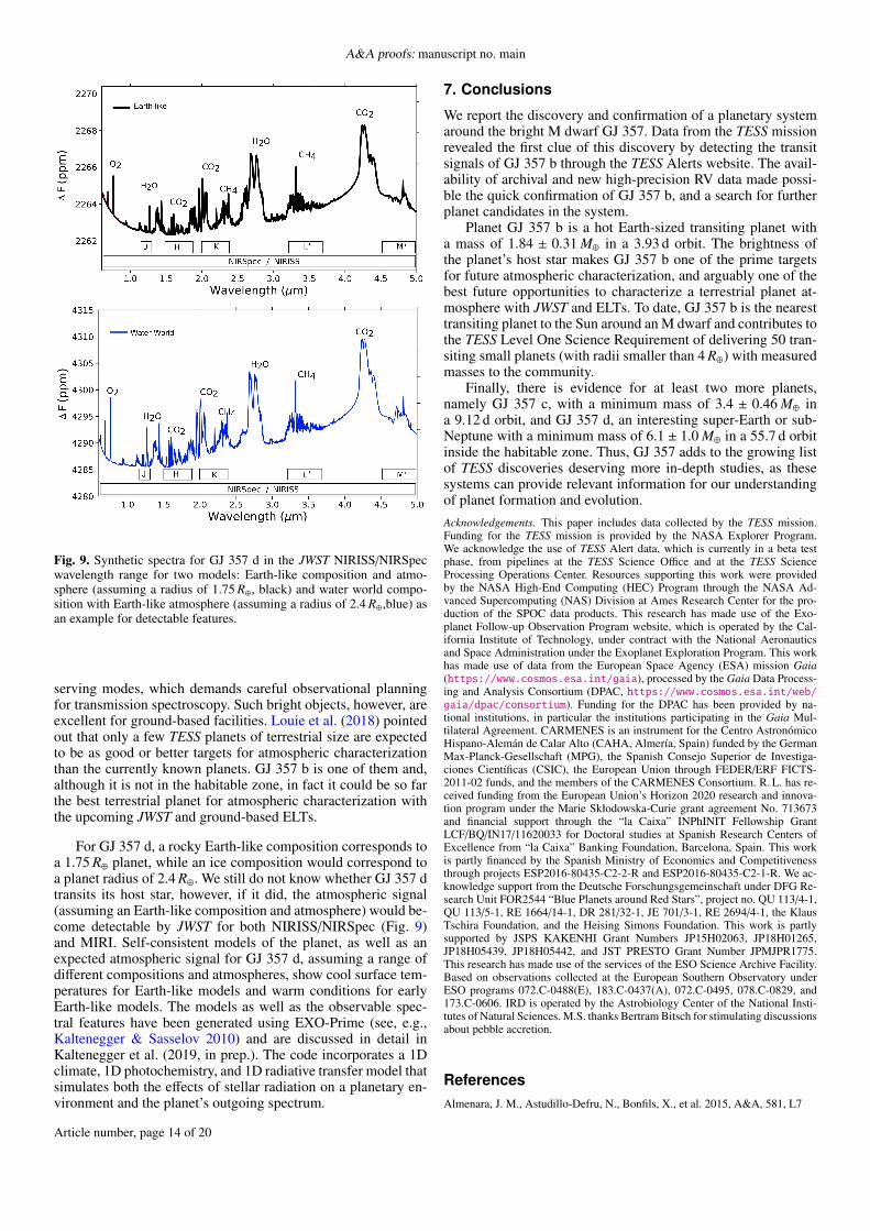
Fig. 9. Synthetic spectra for GJ 357 d in the JWST NIRISS/NIRSpecwavelength range for two models: Earth-like composition and atmo-sphere (assuming a radius of 1.75 R⊕, black) and water world compo-sition with Earth-like atmosphere (assuming a radius of 2.4 R⊕,blue) asan example for detectable features.

serving modes, which demands careful observational planningfor transmission spectroscopy. Such bright objects, however, areexcellent for ground-based facilities. Louie et al. (2018) pointedout that only a few TESS planets of terrestrial size are expectedto be as good or better targets for atmospheric characterizationthan the currently known planets. GJ 357 b is one of them and,although it is not in the habitable zone, in fact it could be so farthe best terrestrial planet for atmospheric characterization withthe upcoming JWST and ground-based ELTs.

For GJ 357 d, a rocky Earth-like composition corresponds toa 1.75 R⊕ planet, while an ice composition would correspond toa planet radius of 2.4 R⊕. We still do not know whether GJ 357 dtransits its host star, however, if it did, the atmospheric signal(assuming an Earth-like composition and atmosphere) would be-come detectable by JWST for both NIRISS/NIRSpec (Fig. 9)and MIRI. Self-consistent models of the planet, as well as anexpected atmospheric signal for GJ 357 d, assuming a range ofdifferent compositions and atmospheres, show cool surface tem-peratures for Earth-like models and warm conditions for earlyEarth-like models. The models as well as the observable spec-tral features have been generated using EXO-Prime (see, e.g.,Kaltenegger & Sasselov 2010) and are discussed in detail inKaltenegger et al. (2019, in prep.). The code incorporates a 1Dclimate, 1D photochemistry, and 1D radiative transfer model thatsimulates both the effects of stellar radiation on a planetary en-vironment and the planet’s outgoing spectrum.

7. Conclusions

We report the discovery and confirmation of a planetary systemaround the bright M dwarf GJ 357. Data from the TESS missionrevealed the first clue of this discovery by detecting the transitsignals of GJ 357 b through the TESS Alerts website. The avail-ability of archival and new high-precision RV data made possi-ble the quick confirmation of GJ 357 b, and a search for furtherplanet candidates in the system.

Planet GJ 357 b is a hot Earth-sized transiting planet witha mass of 1.84 ± 0.31 M⊕ in a 3.93 d orbit. The brightness ofthe planet’s host star makes GJ 357 b one of the prime targetsfor future atmospheric characterization, and arguably one of thebest future opportunities to characterize a terrestrial planet at-mosphere with JWST and ELTs. To date, GJ 357 b is the nearesttransiting planet to the Sun around an M dwarf and contributes tothe TESS Level One Science Requirement of delivering 50 tran-siting small planets (with radii smaller than 4 R⊕) with measuredmasses to the community.

Finally, there is evidence for at least two more planets,namely GJ 357 c, with a minimum mass of 3.4 ± 0.46 M⊕ ina 9.12 d orbit, and GJ 357 d, an interesting super-Earth or sub-Neptune with a minimum mass of 6.1 ± 1.0 M⊕ in a 55.7 d orbitinside the habitable zone. Thus, GJ 357 adds to the growing listof TESS discoveries deserving more in-depth studies, as thesesystems can provide relevant information for our understandingof planet formation and evolution.Acknowledgements. This paper includes data collected by the TESS mission.Funding for the TESS mission is provided by the NASA Explorer Program.We acknowledge the use of TESS Alert data, which is currently in a beta testphase, from pipelines at the TESS Science Office and at the TESS ScienceProcessing Operations Center. Resources supporting this work were providedby the NASA High-End Computing (HEC) Program through the NASA Ad-vanced Supercomputing (NAS) Division at Ames Research Center for the pro-duction of the SPOC data products. This research has made use of the Exo-planet Follow-up Observation Program website, which is operated by the Cal-ifornia Institute of Technology, under contract with the National Aeronauticsand Space Administration under the Exoplanet Exploration Program. This workhas made use of data from the European Space Agency (ESA) mission Gaia(https://www.cosmos.esa.int/gaia), processed by the Gaia Data Process-ing and Analysis Consortium (DPAC, https://www.cosmos.esa.int/web/gaia/dpac/consortium). Funding for the DPAC has been provided by na-tional institutions, in particular the institutions participating in the Gaia Mul-tilateral Agreement. CARMENES is an instrument for the Centro AstronómicoHispano-Alemán de Calar Alto (CAHA, Almería, Spain) funded by the GermanMax-Planck-Gesellschaft (MPG), the Spanish Consejo Superior de Investiga-ciones Científicas (CSIC), the European Union through FEDER/ERF FICTS-2011-02 funds, and the members of the CARMENES Consortium. R. L. has re-ceived funding from the European Union’s Horizon 2020 research and innova-tion program under the Marie Skłodowska-Curie grant agreement No. 713673and financial support through the “la Caixa” INPhINIT Fellowship GrantLCF/BQ/IN17/11620033 for Doctoral studies at Spanish Research Centers ofExcellence from “la Caixa” Banking Foundation, Barcelona, Spain. This workis partly financed by the Spanish Ministry of Economics and Competitivenessthrough projects ESP2016-80435-C2-2-R and ESP2016-80435-C2-1-R. We ac-knowledge support from the Deutsche Forschungsgemeinschaft under DFG Re-search Unit FOR2544 “Blue Planets around Red Stars”, project no. QU 113/4-1,QU 113/5-1, RE 1664/14-1, DR 281/32-1, JE 701/3-1, RE 2694/4-1, the KlausTschira Foundation, and the Heising Simons Foundation. This work is partlysupported by JSPS KAKENHI Grant Numbers JP15H02063, JP18H01265,JP18H05439, JP18H05442, and JST PRESTO Grant Number JPMJPR1775.This research has made use of the services of the ESO Science Archive Facility.Based on observations collected at the European Southern Observatory underESO programs 072.C-0488(E), 183.C-0437(A), 072.C-0495, 078.C-0829, and173.C-0606. IRD is operated by the Astrobiology Center of the National Insti-tutes of Natural Sciences. M.S. thanks Bertram Bitsch for stimulating discussionsabout pebble accretion.

ReferencesAlmenara, J. M., Astudillo-Defru, N., Bonfils, X., et al. 2015, A&A, 581, L7

Article number, page 14 of 20

R. Luque et al.: Planetary system around GJ 357

Alonso-Floriano, F. J., Morales, J. C., Caballero, J. A., et al. 2015, A&A, 577,A128

Ambikasaran, S., Foreman-Mackey, D., Greengard, L., Hogg, D. W., & O’Neil,M. 2015, IEEE Transactions on Pattern Analysis and Machine Intelligence,38, 252

Anglada-Escudé, G., Amado, P. J., Barnes, J., et al. 2016, Nature, 536, 437Anglada-Escudé, G., Tuomi, M., Gerlach, E., et al. 2013, A&A, 556, A126Astudillo-Defru, N., Delfosse, X., Bonfils, X., et al. 2017, A&A, 600, A13Bakos, G., Noyes, R. W., Kovács, G., et al. 2004, PASP, 116, 266Batalha, N. E., Lewis, N. K., Line, M. R., Valenti, J., & Stevenson, K. 2018, ApJ,

856, L34Berta-Thompson, Z. K., Irwin, J., Charbonneau, D., et al. 2015, Nature, 527, 204Birnstiel, T., Klahr, H., & Ercolano, B. 2012, A&A, 539, A148Bitsch, B., Izidoro, A., Johansen, A., et al. 2019, A&A, 623, A88Bonfils, X., Almenara, J. M., Cloutier, R., et al. 2018, A&A, 618, A142Bonfils, X., Delfosse, X., Udry, S., et al. 2013, A&A, 549, A109Boro Saikia, S., Marvin, C. J., Jeffers, S. V., et al. 2018, A&A, 616, A108Broeg, C., Fortier, A., Ehrenreich, D., et al. 2013, in European Physical Journal

Web of Conferences, Vol. 47, European Physical Journal Web of Conferences,03005

Brown, T. M., Baliber, N., Bianco, F. B., et al. 2013, Publications of the Astro-nomical Society of the Pacific, 125, 1031

Buchhave, L. A., Dressing, C. D., Dumusque, X., et al. 2016, AJ, 152, 160Buchner, J., Georgakakis, A., Nandra, K., et al. 2014, A&A, 564, A125Butler, R. P., Marcy, G. W., Williams, E., et al. 1996, PASP, 108, 500Butler, R. P., Vogt, S. S., Laughlin, G., et al. 2017, AJ, 153, 208Charbonneau, D., Irwin, J., Nutzman, P., & Falco, E. E. 2008, in Bulletin of

the American Astronomical Society, Vol. 40, American Astronomical SocietyMeeting Abstracts #212, 242

Chiang, E. I. & Goldreich, P. 1997, ApJ, 490, 368Christiansen, J. L., Vanderburg, A., Burt, J., et al. 2017, AJ, 154, 122Ciesla, F. J. & Cuzzi, J. N. 2006, Icarus, 181, 178Cloutier, R., Astudillo-Defru, N., Doyon, R., et al. 2017, A&A, 608, A35Collins, K. A., Kielkopf, J. F., Stassun, K. G., & Hessman, F. V. 2017, AJ, 153,

77Cortés Contreras , M. 2016, PhD thesis, Departamento de Astrofísica, Facul-

tad de Ciencias Físicas, Universidad Complutense de Madrid, 28040 Madrid,Spain

Cortés-Contreras, M., Béjar, V. J. S., Caballero, J. A., et al. 2017, A&A, 597,A47

Crane, J. D., Shectman, S. A., Butler, R. P., et al. 2010, in Proc. SPIE, Vol. 7735,Ground-based and Airborne Instrumentation for Astronomy III, 773553

Cumming, A., Butler, R. P., Marcy, G. W., et al. 2008, Publications of the Astro-nomical Society of the Pacific, 120, 531

Cuzzi, J. N. & Zahnle, K. J. 2004, ApJ, 614, 490Dai, F., Masuda, K., & Winn, J. N. 2018, ApJ, 864, L38Díez Alonso, E., Caballero, J. A., Montes, D., et al. 2019, A&A, 621, A126Dittmann, J. A., Irwin, J. M., Charbonneau, D., et al. 2017, Nature, 544, 333Drake, A. J., Graham, M. J., Djorgovski, S. G., et al. 2014, ApJS, 213, 9Endl, M., Kürster, M., & Els, S. 2000, A&A, 362, 585Espinoza, N. 2018, Research Notes of the American Astronomical Society, 2,

209Espinoza, N., Brahm, R., Henning, T., et al. 2019, arXiv e-prints,

arXiv:1903.07694Espinoza, N. & Jordán, A. 2015, MNRAS, 450, 1879Espinoza, N., Kossakowski, D., & Brahm, R. 2018, arXiv e-prints,

arXiv:1812.08549Feroz, F., Hobson, M. P., & Bridges, M. 2009, MNRAS, 398, 1601Foreman-Mackey, D., Agol, E., Ambikasaran, S., & Angus, R. 2017, celerite:

Scalable 1D Gaussian Processes in C++, Python, and JuliaFrance, K., Loyd, R. P., Youngblood, A., et al. 2016, The Astrophysical Journal,

820, 89Fulton, B. J., Petigura, E. A., Blunt, S., & Sinukoff, E. 2018, Publications of the

Astronomical Society of the Pacific, 130, 044504Fulton, B. J., Petigura, E. A., Howard, A. W., et al. 2017, AJ, 154, 109Gaia Collaboration, Brown, A. G. A., Vallenari, A., et al. 2018, A&A, 616, A1Gandolfi, D., Barragán, O., Hatzes, A. P., et al. 2017, AJ, 154, 123Gilliland, R. L., Marcy, G. W., Rowe, J. F., et al. 2013, ApJ, 766, 40Gillon, M., Jehin, E., Lederer, S. M., et al. 2016, Nature, 533, 221Gillon, M., Triaud, A. H. M. J., Demory, B.-O., et al. 2017, Nature, 542, 456Gliese, W. 1957, Astronomisches Rechen-Institut Heidelberg Mitteilungen Serie

A, 8, 1Greene, T. P., Line, M. R., Montero, C., et al. 2016, The Astrophysical Journal,

817, 17Günther, M. N., Pozuelos, F. J., Dittmann, J. A., et al. 2019, arXiv e-prints

[arXiv:1903.06107]Harpsøe, K. B. W., Hardis, S., Hinse, T. C., et al. 2013, A&A, 549, A10Hawley, S. L., Gizis, J. E., & Reid, I. N. 1996, AJ, 112, 2799Hayano, Y., Takami, H., Oya, S., et al. 2010, in Proc. SPIE, Vol. 7736, Adaptive

Optics Systems II, 77360N

Hébrard, E., Dobrijevic, M., Loison, J.-C., Bergeat, A., & Hickson, K. 2012,Astronomy & Astrophysics, 541, A21

Iyer, A. R., Swain, M. R., Zellem, R. T., et al. 2016, ApJ, 823, 109Jenkins, J. M., Twicken, J. D., McCauliff, S., et al. 2016, in Proc. SPIE, Vol.

9913, Software and Cyberinfrastructure for Astronomy IV, 99133EJensen, E. 2013, Tapir: A web interface for transit/eclipse observability, Astro-

physics Source Code LibraryJódar, E., Pérez-Garrido, A., Díaz-Sánchez, A., et al. 2013, MNRAS, 429, 859Johansen, A., Oishi, J. S., Mac Low, M.-M., et al. 2007, Nature, 448, 1022Kaltenegger, L. & Sasselov, D. 2010, ApJ, 708, 1162Kasting, J. F., Whitmire, D. P., & Reynolds, R. T. 1993, Icarus, 101, 108Kawashima, Y. & Rugheimer, S. 2019, AJ, 157, 213Kempton, E. M.-R., Bean, J. L., Louie, D. R., et al. 2018, PASP, 130, 114401Kipping, D. M. 2013, MNRAS, 435, 2152Klahr, H. & Bodenheimer, P. 2006, The Astrophysical Journal, 639, 432Kochanek, C. S., Shappee, B. J., Stanek, K. Z., et al. 2017, PASP, 129, 104502Kopparapu, R. K., Ramirez, R. M., SchottelKotte, J., et al. 2014, ApJ, 787, L29Kostov, V. B., Schlieder, J. E., Barclay, T., et al. 2019, AJ, 158, 32Kotani, T., Tamura, M., Nishikawa, J., et al. 2018, in Society of Photo-Optical

Instrumentation Engineers (SPIE) Conference Series, Vol. 10702, Ground-based and Airborne Instrumentation for Astronomy VII, 1070211

Kreidberg, L. 2015, Publications of the Astronomical Society of the Pacific, 127,1161

Kreidberg, L., Bean, J. L., Désert, J.-M., et al. 2014, Nature, 505, 69Kürster, M., Endl, M., Rouesnel, F., et al. 2003, A&A, 403, 1077Labadie, L., Rebolo, R., Femenía, B., et al. 2010, in Proc. SPIE, Vol. 7735,

Ground-based and Airborne Instrumentation for Astronomy III, 77350XLambrechts, M., Johansen, A., & Morbidelli, A. 2014, A&A, 572, A35Lendl, M., Ehrenreich, D., Turner, O. D., et al. 2017, A&A, 603, L5Lenz, C. T., Klahr, H., & Birnstiel, T. 2019, ApJ, 874, 36Levison, H. F., Kretke, K. A., & Duncan, M. J. 2015, Nature, 524, 322Li, J., Tenenbaum, P., Twicken, J. D., et al. 2019, PASP, 131, 024506Louie, D. R., Deming, D., Albert, L., et al. 2018, PASP, 130, 044401Lovis, C. & Pepe, F. 2007, A&A, 468, 1115Luque, R., Nowak, G., Pallé, E., et al. 2018, A&A, 620, A171Luyten, W. J. 1942, Publications of the Astronomical Observatory University of

Minnesota, 2, 242Mandel, K. & Agol, E. 2002, ApJ, 580, L171Marcy, G. W., Isaacson, H., Howard, A. W., et al. 2014, ApJS, 210, 20Maxted, P. F. L., Anderson, D. R., Collier Cameron, A., et al. 2011, PASP, 123,

547Mayor, M., Pepe, F., Queloz, D., et al. 2003, The Messenger, 114, 20Ment, K., Dittmann, J. A., Astudillo-Defru, N., et al. 2019, AJ, 157, 32Meschiari, S., Wolf, A. S., Rivera, E., et al. 2009, PASP, 121, 1016Molaverdikhani, K., Henning, T., & Mollière, P. 2019, The Astrophysical Jour-

nal, 873, 32Mollière, P., Wardenier, J. P., van Boekel, R., et al. 2019, A&A, 627, A67Montes, D., López-Santiago, J., Gálvez, M. C., et al. 2001, MNRAS, 328, 45Mordasini, C., Alibert, Y., Klahr, H., & Henning, T. 2012, A&A, 547, A111Motalebi, F., Udry, S., Gillon, M., et al. 2015, A&A, 584, A72Moutou, C., Hébrard, E. M., Morin, J., et al. 2017, MNRAS, 472, 4563Ofir, A. 2014, A&A, 561, A138Ofir, A., Dreizler, S., Zechmeister, M., & Husser, T.-O. 2014, A&A, 561, A103Ofir, A., Xie, J.-W., Jiang, C.-F., Sari, R., & Aharonson, O. 2018, The Astro-

physical Journal Supplement Series, 234, 9Ormel, C. W. & Klahr, H. H. 2010, A&A, 520, A43Ormel, C. W., Liu, B., & Schoonenberg, D. 2017, A&A, 604, A1Oscoz, A., Rebolo, R., López, R., et al. 2008, in Proc. SPIE, Vol. 7014, Ground-

based and Airborne Instrumentation for Astronomy II, 701447Otor, O. J., Montet, B. T., Johnson, J. A., et al. 2016, AJ, 152, 165Pallé, E., Zapatero Osorio, M. R., Barrena, R., Montañés-Rodríguez, P., &

Martín, E. L. 2009, Nature, 459, 814Parviainen, H. 2015, MNRAS, 450, 3233Pojmanski, G. 2002, Acta Astron., 52, 397Pollacco, D. L., Skillen, I., Collier Cameron, A., et al. 2006, PASP, 118, 1407Quinn, S. N., White, T. R., Latham, D. W., et al. 2015, ApJ, 803, 49Quirrenbach, A., Amado, P. J., Caballero, J. A., et al. 2014, in Proc. SPIE, Vol.

9147, Ground-based and Airborne Instrumentation for Astronomy V, 91471FQuirrenbach, A., Amado, P. J., Ribas, I., et al. 2018, in Society of Photo-Optical

Instrumentation Engineers (SPIE) Conference Series, Vol. 10702, Ground-based and Airborne Instrumentation for Astronomy VII, 107020W

Reiners, A., Zechmeister, M., Caballero, J. A., et al. 2018, A&A, 612, A49Ribas, I., Tuomi, M., Reiners, A., et al. 2018, Nature, 563, 365Ricker, G. R., Winn, J. N., Vanderspek, R., et al. 2015, Journal of Astronomical

Telescopes, Instruments, and Systems, 1, 014003Rowe, J. F., Bryson, S. T., Marcy, G. W., et al. 2014, ApJ, 784, 45Sarkis, P., Henning, T., Kürster, M., et al. 2018, AJ, 155, 257Schöfer, P., Jeffers, S. V., Reiners, A., et al. 2019, A&A, 623, A44Schoonenberg, D. & Ormel, C. W. 2017, A&A, 602, A21Schweitzer, A., Passegger, V. M., Cifuentes, C., et al. 2019, A&A, 625, A68

Article number, page 15 of 20

A&A proofs: manuscript no. main

Sinukoff, E., Howard, A. W., Petigura, E. A., et al. 2016, ApJ, 827, 78

Skrutskie, M. F., Cutri, R. M., Stiening, R., et al. 2006, AJ, 131, 1163

Smith, J. C., Stumpe, M. C., Van Cleve, J. E., et al. 2012, PASP, 124, 1000

Southworth, J. 2011, MNRAS, 417, 2166

Speagle, J. S. 2019, arXiv e-prints, arXiv:1904.02180

Stassun, K. G., Oelkers, R. J., Pepper, J., et al. 2018, AJ, 156, 102

Stelzer, B., Marino, A., Micela, G., López-Santiago, J., & Liefke, C. 2013, MN-RAS, 431, 2063

Stevenson, D. J. & Lunine, J. I. 1988, Icarus, 75, 146

Stumpe, M. C., Smith, J. C., Catanzarite, J. H., et al. 2014, PASP, 126, 100

Stumpe, M. C., Smith, J. C., Van Cleve, J. E., et al. 2012, PASP, 124, 985

Suárez Mascareño, A., Rebolo, R., González Hernández, J. I., & Esposito, M.2015, MNRAS, 452, 2745

Sullivan, P. W., Winn, J. N., Berta-Thompson, Z. K., et al. 2015, ApJ, 809, 77

Tal-Or, L., Trifonov, T., Zucker, S., Mazeh, T., & Zechmeister, M. 2019, MN-RAS, 484, L8

ter Braak, C. J. F. & Vrugt, J. A. 2008, Statistics and Computing, 18, 435

Trifonov, T., Kürster, M., Zechmeister, M., et al. 2018, A&A, 609, A117

Trotta, R. 2008, Contemporary Physics, 49, 71

Tuomi, M. & Anglada-Escudé, G. 2013, A&A, 556, A111

Twicken, J. D., Catanzarite, J. H., Clarke, B. D., et al. 2018, PASP, 130, 064502

Udry, S., Bonfils, X., Delfosse, X., et al. 2007, A&A, 469, L43

Van Eylen, V., Agentoft, C., Lundkvist, M. S., et al. 2018, MNRAS, 479, 4786

Vanderspek, R., Huang, C. X., Vanderburg, A., et al. 2019, ApJ, 871, L24

Venot, O., Hébrard, E., Agúndez, M., et al. 2012, Astronomy & Astrophysics,546, A43

Vogt, S. S., Allen, S. L., Bigelow, B. C., et al. 1994, in Proc. SPIE, Vol. 2198,Instrumentation in Astronomy VIII, ed. D. L. Crawford & E. R. Craine, 362

Vogt, S. S., Marcy, G. W., Butler, R. P., & Apps, K. 2000, ApJ, 536, 902

Wakeford, H. R., Sing, D. K., Kataria, T., et al. 2017, Science, 356, 628

Wozniak, P. R., Vestrand, W. T., Akerlof, C. W., et al. 2004, AJ, 127, 2436

Zacharias, N., Finch, C. T., Girard, T. M., et al. 2013, AJ, 145, 44

Zechmeister, M. & Kürster, M. 2009, A&A, 496, 577

Zechmeister, M., Kürster, M., & Endl, M. 2009, A&A, 505, 859

Zechmeister, M., Reiners, A., Amado, P. J., et al. 2018, A&A, 609, A12

Zeng, L., Sasselov, D. D., & Jacobsen, S. B. 2016, ApJ, 819, 127

1 Instituto de Astrofísica de Canarias (IAC), 38205 La Laguna, Tener-ife, Spain; e-mail: rluque@iac.es

2 Departamento de Astrofísica, Universidad de La Laguna (ULL),38206, La Laguna, Tenerife, Spain

3 Max-Planck-Institut für Astronomie, Königstuhl 17, 69117 Heidel-berg, Germany

4 Institut für Astrophysik, Georg-August-Universität, Friedrich-Hund-Platz 1, 37077 Göttingen, Germany

5 Landessternwarte, Zentrum für Astronomie der Universität Heidel-berg, Königstuhl 12, 69117 Heidelberg, Germany

6 Kavli Institute for Astrophysics and Space Research, MassachusettsInstitute of Technology, Cambridge, MA 02139, USA

7 School of Physics and Astronomy, Queen Mary, University of Lon-don, 327 Mile End Road, London, E1 4NS

8 Instituto de Astrofísica de Andalucía (IAA-CSIC), Glorieta de laAstronomía s/n, 18008 Granada, Spain

9 Centro de Astrobiología (CSIC-INTA), ESAC, Camino bajo delcastillo s/n, 28692 Villanueva de la Cañada, Madrid, Spain

10 Harvard-Smithsonian Center for Astrophysics, 60 Garden St, Cam-bridge, MA 02138, USA

11 Department of Physics and Astronomy, Vanderbilt University,Nashville, TN 37235, USA

12 Departamento de Física de la Tierra y Astrofísica & IPARCOS-UCM (Instituto de Física de Partículas y del Cosmos de la UCM),

Facultad de Ciencias Físicas, Universidad Complutense de Madrid,28040 Madrid, Spain

13 Department of Exploitation and Exploration of Mines, University ofOviedo, Oviedo, Spain

14 Department of Terrestrial Magnetism, Carnegie Institution for Sci-ence, 5241 Broad Branch Road, NW, Washington, DC 20015, USA

15 Thüringer Landessternwarte Tautenburg, Sternwarte 5, 07778 Taut-enburg, Germany

16 Astrophysics Group, Keele University, Staffordshire, ST5 5BG, UK17 Carl Sagan Institute, Cornell University, Ithaca, NY 14853, USA18 Astrobiology Center, 2-21-1 Osawa, Mitaka, Tokyo 181-8588, Japan19 JST, PRESTO, 2-21-1 Osawa, Mitaka, Tokyo 181-8588, Japan20 National Astronomical Observatory of Japan, 2-21-1 Osawa, Mi-

taka, Tokyo 181-8588, Japan21 Weizmann Institute of Science, 234 Herzl Street, Rehovot 761001,

Israel22 Department of Astrophysical Sciences, Princeton University, 4 Ivy

Lane, Princeton, NJ 08544, USA23 Centro de Astrobiología (CSIC-INTA), Carretera de Ajalvir km 4,

28850 Torrejón de Ardoz, Madrid, Spain24 Department of Astronomy and Astrophysics, University of Califor-

nia, Santa Cruz, CA 95064, USA25 SETI Institute, Mountain View, CA 94043, USA26 NASA Ames Research Center, Moffett Field, CA, 94035, USA27 Key Laboratory of Planetary Sciences, Purple Mountain Observa-

tory, Chinese Academy of Sciences, Nanjing 210008, China28 Observatories of the Carnegie Institution for Science, 813 Santa Bar-

bara Street, Pasadena, CA 91101, USA29 Department of Astronomy, The University of California, Berkeley,

CA 94720, USA30 Institut de Ciències de l’Espai (ICE, CSIC), Campus UAB, C/Can

Magrans s/n, 08193 Bellaterra, Spain31 Institut d’Estudis Espacials de Catalunya (IEEC), 08034 Barcelona,

Spain32 The Maury Lewin Astronomical Observatory, Glendora, California

91741, USA33 Proto-Logic LLC, 1718 Euclid Street NW, Washington, DC 20009,

USA34 Hamburger Sternwarte, Universität Hamburg, Gojenbergsweg 112,

21029 Hamburg, Germany35 Centro Astronómico Hispano-Alemán (CSIC-MPG), Observatorio

Astronómico de Calar Alto, Sierra de los Filabres-04550 Gérgal,Almería, Spain

36 School of Physical Sciences, The Open University, Milton KeynesMK7 6AA, UK

37 Department of Earth, Atmospheric and Planetary Sciences, Mas-sachusetts Institute of Technology, Cambridge, MA 02139, USA

38 Department of Aeronautics and Astronautics, MIT, 77 Mas-sachusetts Avenue, Cambridge, MA 02139, USA

39 Department of Astronomy, The University of Tokyo, 7-3-1 Hongo,Bunkyo-ku, Tokyo 113-0033, Japan

40 Torres Fellow41 NASA Hubble Fellow

Article number, page 16 of 20

R. Luque et al.: Planetary system around GJ 357

Appendix A: Joint fit priors.

Article number, page 17 of 20

A&A proofs: manuscript no. main

Table A.1. Priors used for the joint fit model 3pl+GPexp presented in Sect. 5.2.3 using juliet. The prior labels of N , U, and J representnormal, uniform, and Jeffrey’s distributions. The parametrization for (p, b) using (r1, r2) (Espinoza 2018) and the linear (q1) and quadratic (q1, q2)limb-darkening parametrization (Kipping 2013) are both described in Sect. 5.2.1.

Parameter name Prior Units Description

Stellar parametersρ? N(13600, 17002) kg m −3 Stellar density.

Planet parametersPb N(3.93079, 0.0012) d Period of planet b.Pc N(9.1, 0.12) d Period of planet c.Pd N(55.7, 0.52) d Period of planet d.t0,b − 2450000 N(8517.99, 0.12) d Time of transit-center of planet b.t0,c − 2450000 U(8312, 8318) d Time of transit-center of planet c.t0,d − 2450000 U(8310, 8340) d Time of transit-center of planet d.r1,b U(0, 1) . . . Parametrization for p and b.r2,b U(0, 1) . . . Parametrization for p and b.Kb U(0, 10) m s−1 RV semi-amplitude of planet b.Kc U(0, 10) m s−1 RV semi-amplitude of planet c.Kd U(0, 10) m s−1 RV semi-amplitude of planet d.S1,b,c,d =

√eb,c,d sinωb,c,d 0.0 (fixed) . . . Parametrization for e and ω.

S2,b,c,d =√

eb,c,d cosωb,c,d 0.0 (fixed) . . . Parametrization for e and ω.Photometry parameters

DTESS 1.0 (fixed) . . . Dilution factor.MTESS N(0, 0.12) ppm Relative flux offset for TESS.σTESS U(1, 500) ppm Extra jitter term for TESS.q1,TESS U(0, 1) . . . Quadratic limb-darkening parametrization for TESS.q2,TESS U(0, 1) . . . Quadratic limb-darkening parametrization for TESS.MLCO N(0, 0.12) ppm Relative flux offset for LCO.σLCO U(1, 2000) ppm Extra jitter term for LCO.q1,LCO U(0, 1) . . . Linear limb-darkening parametrization for LCO.

RV parametersµHIRES U(−10, 10) m s−1 Systemic velocity for HIRES.σHIRES U(0, 10) m s−1 Extra jitter term for HIRES.µUVES U(−10, 10) m s−1 Systemic velocity for UVES.σUVES U(0, 10) m s−1 Extra jitter term for UVES.µHARPS U(−10, 10) m s−1 Systemic velocity for HARPS.σHARPS U(0, 10) m s−1 Extra jitter term for HARPS.µPFSpre U(−10, 10) m s−1 Systemic velocity for PFSpre.σPFSpre U(0, 10) m s−1 Extra jitter term for PFSpre.µPFSpost U(−10, 10) m s−1 Systemic velocity for PFSpost.σPFSpost U(0, 10) m s−1 Extra jitter term for PFSpost.µCARMENES U(−10, 10) m s−1 Systemic velocity for CARMENES.σCARMENES U(0, 10) m s−1 Extra jitter term for CARMENES.

GP hyperparametersσGP,TESS J(10−2, 500) ppm Amplitude of GP component for TESS.TGP,TESS J(10−2, 1000) d Length scale of GP component for TESS.σGP,RV J(0.1, 10) m s−1 Amplitude of GP component for the RVs.TGP,RV J(10−4, 10) d Length scale of GP component for the RVs.

Article number, page 18 of 20

R. Luque et al.: Planetary system around GJ 357

Appendix B: RV time series of best joint fit

Article number, page 19 of 20

A&A proofs: manuscript no. main

10

5

0

5

10

RV

(m/s

)

HIRES UVES HARPS PFSPRE CARMENES PFSPOST

0 500 1000 1500 2000 250010

0

10

O-C

10

5

0

5

10

RV

(m/s

)

3000 3500 4000 4500 5000 550010

0

10

O-C

10

5

0

5

10

RV

(m/s

)

7000 7500 8000 8500 9000Time (BJD - 2450839)

10

0

10

O-C

Fig. B.1. RV measurements as a function of time along with the residuals obtained from subtracting our median best joint fit model (black line)and the 68%, 95%, and 99% posterior bands (shown in blue). The color coding of the datapoints for each instrument is shown at the top.

Article number, page 20 of 20