Astronomy & Astrophysics manuscript no. planck˙boosting c© ESO 2015July 23, 2015

Planck 2013 results. XXVII. Doppler boosting of the CMB:Eppur si muove?

Planck Collaboration: N. Aghanim56, C. Armitage-Caplan85, M. Arnaud69, M. Ashdown66,6, F. Atrio-Barandela16, J. Aumont56, C. Baccigalupi79,A. J. Banday87,9, R. B. Barreiro63, J. G. Bartlett1,64, K. Benabed57,86, A. Benoit-Levy22,57,86, J.-P. Bernard87,9, M. Bersanelli34,47, P. Bielewicz87,9,79,

J. Bobin69, J. J. Bock64,10, J. R. Bond8, J. Borrill12,83, F. R. Bouchet57,86, M. Bridges66,6,60, C. Burigana46,32, R. C. Butler46, J.-F. Cardoso70,1,57,A. Catalano71,68, A. Challinor60,66,11, A. Chamballu69,13,56, H. C. Chiang26,7, L.-Y Chiang59, P. R. Christensen76,37, D. L. Clements54,

L. P. L. Colombo21,64, F. Couchot67, B. P. Crill64,77, A. Curto6,63, F. Cuttaia46, L. Danese79, R. D. Davies65, R. J. Davis65, P. de Bernardis33, A. deRosa46, G. de Zotti42,79, J. Delabrouille1, J. M. Diego63, S. Donzelli47, O. Dore64,10, X. Dupac39, G. Efstathiou60, T. A. Enßlin74, H. K. Eriksen61,

F. Finelli46,48, O. Forni87,9, M. Frailis44, E. Franceschi46, S. Galeotta44, K. Ganga1, M. Giard87,9, G. Giardino40, J. Gonzalez-Nuevo63,79,K. M. Gorski64,89, S. Gratton66,60, A. Gregorio35,44,50, A. Gruppuso46, F. K. Hansen61, D. Hanson75,64,8, D. L. Harrison60,66, G. Helou10,

S. R. Hildebrandt10, E. Hivon57,86, M. Hobson6, W. A. Holmes64, W. Hovest74, K. M. Huffenberger24, W. C. Jones26, M. Juvela25, E. Keihanen25,R. Keskitalo19,12, T. S. Kisner73, J. Knoche74, L. Knox28, M. Kunz15,56,3, H. Kurki-Suonio25,41, A. Lahteenmaki2,41, J.-M. Lamarre68,

A. Lasenby6,66, R. J. Laureijs40, C. R. Lawrence64, R. Leonardi39, A. Lewis23, M. Liguori31, P. B. Lilje61, M. Linden-Vørnle14,M. Lopez-Caniego63, P. M. Lubin29, J. F. Macıas-Perez71, N. Mandolesi46,5,32, M. Maris44, D. J. Marshall69, P. G. Martin8,

E. Martınez-Gonzalez63, S. Masi33, M. Massardi45, S. Matarrese31, P. Mazzotta36, P. R. Meinhold29, A. Melchiorri33,49, L. Mendes39,M. Migliaccio60,66, S. Mitra53,64, A. Moneti57, L. Montier87,9, G. Morgante46, D. Mortlock54, A. Moss81, D. Munshi80, P. Naselsky76,37, F. Nati33,P. Natoli32,4,46, H. U. Nørgaard-Nielsen14, F. Noviello65, D. Novikov54, I. Novikov76, S. Osborne84, C. A. Oxborrow14, L. Pagano33,49, F. Pajot56,

D. Paoletti46,48, F. Pasian44, G. Patanchon1, O. Perdereau67, F. Perrotta79, F. Piacentini33, E. Pierpaoli21, D. Pietrobon64, S. Plaszczynski67,E. Pointecouteau87,9, G. Polenta4,43, N. Ponthieu56,51, L. Popa58, G. W. Pratt69, G. Prezeau10,64, J.-L. Puget56, J. P. Rachen18,74, W. T. Reach88,M. Reinecke74, S. Ricciardi46, T. Riller74, I. Ristorcelli87,9, G. Rocha64,10, C. Rosset1, J. A. Rubino-Martın62,38, B. Rusholme55, D. Santos71,

G. Savini78, D. Scott20 ??, M. D. Seiffert64,10, E. P. S. Shellard11, L. D. Spencer80, R. Sunyaev74,82, F. Sureau69, A.-S. Suur-Uski25,41,J.-F. Sygnet57, J. A. Tauber40, D. Tavagnacco44,35, L. Terenzi46, L. Toffolatti17,63, M. Tomasi34,47, M. Tristram67, M. Tucci15,67, M. Turler52,

L. Valenziano46, J. Valiviita41,25,61, B. Van Tent72, P. Vielva63, F. Villa46, N. Vittorio36, L. A. Wade64, B. D. Wandelt57,86,30, M. White27, D. Yvon13,A. Zacchei44, J. P. Zibin20, and A. Zonca29

(Affiliations can be found after the references)

A&A: submitted, 23 March 2013, accepted 3 January 2014.

ABSTRACT

Our velocity relative to the rest frame of the cosmic microwave background (CMB) generates a dipole temperature anisotropy on the sky whichhas been well measured for more than 30 years, and has an accepted amplitude of v/c = 1.23 × 10−3, or v = 369 km s−1. In addition to thissignal generated by Doppler boosting of the CMB monopole, our motion also modulates and aberrates the CMB temperature fluctuations (as wellas every other source of radiation at cosmological distances). This is an order 10−3 effect applied to fluctuations which are already one part inroughly 105, so it is quite small. Nevertheless, it becomes detectable with the all-sky coverage, high angular resolution, and low noise levels of thePlanck satellite. Here we report a first measurement of this velocity signature using the aberration and modulation effects on the CMB temperatureanisotropies, finding a component in the known dipole direction, (l, b) = (264◦, 48◦), of 384 km s−1 ± 78 km s−1 (stat.) ± 115 km s−1 (syst.). This isa significant confirmation of the expected velocity.

Key words. Cosmology: observations – cosmic background radiation – Reference systems – Relativistic processes

1. Introduction

This paper, one of a set associated with the 2013 release ofdata from the Planck† mission (Planck Collaboration I 2014),presents a study of Doppler boosting effects using the small-

? “And yet it moves,” the phrase popularly attributed to GalileoGalilei after being forced to recant his view that the Earth goes aroundthe Sun.?? Corresponding author: Douglas Scott, dscott@phas.ubc.ca.ca† Planck (http://www.esa.int/Planck) is a project of the

European Space Agency (ESA) with instruments provided by two sci-entific consortia funded by ESA member states (in particular the leadcountries France and Italy), with contributions from NASA (USA) andtelescope reflectors provided by a collaboration between ESA and a sci-entific consortium led and funded by Denmark.

scale temperature fluctuations of the Planck cosmic microwavebackground (CMB) maps.

Observations of the relatively large amplitude CMB temper-ature dipole are usually taken to indicate that our Solar Systembarycentre is in motion with respect to the CMB frame (de-fined precisely below). Assuming that the observed tempera-ture dipole is due entirely to Doppler boosting of the CMBmonopole, one infers a velocity v = (369 ± 0.9) km s−1 in thedirection (l, b) = (263.◦99 ± 0.◦14, 48.◦26 ± 0.◦03), on the bound-ary of the constellations of Crater and Leo (Kogut et al. 1993;Fixsen et al. 1996; Hinshaw et al. 2009).

In addition to Doppler boosting of the CMB monopole, ve-locity effects also boost the order 10−5 primordial temperaturefluctuations. There are two observable effects here, both at alevel of β ≡ v/c = 1.23 × 10−3. First, there is a Doppler “mod-

1

arX

iv:1

303.

5087

v3 [

astr

o-ph

.CO

] 2

2 Ju

l 201

5

Planck Collaboration: Doppler boosting of the CMB: Eppur si muove

ulation” effect, which amplifies the apparent temperature fluctu-ations in the velocity direction, and reduces them in the oppo-site direction. This is the same effect which converts a portionof the CMB monopole into the observed dipole. The effect onthe CMB fluctuations is to increase the amplitude of the powerspectrum by approximately 0.25% in the velocity direction, anddecrease it correspondingly in the anti-direction. Second, thereis an “aberration” effect, in which the apparent arrival direc-tion of CMB photons is pushed toward the velocity direction.This effect is small, but non-negligible. The expected velocityinduces a peak deflection of β = 4.′2 and a root-mean-squared(rms) deflection over the sky of 3′, comparable to the effectsof gravitational lensing by large-scale structure, which are dis-cussed in Planck Collaboration XVII (2014). The aberration ef-fect squashes the anisotropy pattern on one side of the sky andstretches it on the other, effectively changing the angular scale.Close to the velocity direction we expect that the power spec-trum of the temperature anisotropies, C`, will be shifted so that,e.g., `= 1000→ `= 1001, while `= 1000→ `= 999 in the anti-direction. In Fig. 1 we plot an exaggerated illustration of theaberration and modulation effects. For completeness we shouldpoint out that there is a third effect, a quadrupole of amplitudeβ2 induced by the dipole (see Kamionkowski & Knox 2003).However, extracting this signal would require extreme levels ofprecision for foreground modelling at the quadrupole scale, andwe do not discuss it further.

In this paper, we will present a measurement of β, exploitingthe distinctive statistical signatures of the aberration and mod-ulation effects on the high-` CMB temperature anisotropies. Inaddition to our interest in making an independent measurementof the velocity signature, the effects which velocity generates onthe CMB fluctuations provide a source of potential bias or con-fusion for several aspects of the Planck data. In particular, ve-locity effects couple to measurements of: primordial “τNL”-typenon-Gaussianity, as discussed in Planck Collaboration XXIV(2014); statistical anisotropy of the primordial CMB fluctua-tions, as discussed in Planck Collaboration XXIII (2014); andgravitational lensing, as discussed in Planck Collaboration XVII(2014). There are also aspects of the Planck analysis for whichvelocity effects are believed to be negligible, but only if they arepresent at the expected level. One example is measurement offNL-type non-Gaussianity, as discussed in Catena et al. (2013).Another example is power spectrum estimation — as discussedabove, velocity effects change the angular scale of the acous-tic peaks in the CMB power spectrum. Averaged over the fullsky this effect is strongly suppressed, as the expansion and con-traction of scales on opposing hemispheres cancel out. Howeverthe application of a sky mask breaks this cancellation to someextent, and can potentially be important for parameter estima-tion (Pereira et al. 2010; Catena & Notari 2013). For the 143and 217 GHz analysis mask used in the fiducial Planck CMBlikelihood (Planck Collaboration XV 2014), the average lensingconvergence field associated with the aberration effect (on theportion of the sky which is unmasked) has a value which is 13%of its peak value, corresponding to an expected average lensingconvergence of β× 0.13 = 1.5× 10−4. This will shift the angularscale of the acoustic peaks by the same fraction, which is degen-erate with a change in the angular size of the sound horizon atlast scattering, θ∗ (Burles & Rappaport 2006). A 1.5× 10−4 shiftin θ∗ is just under 25% of the Planck uncertainty on this param-eter, as reported in Planck Collaboration XVI (2014) — smallenough to be neglected, though not dramatically so. This there-fore motivates us to test that the observed aberration signal isnot significantly larger than expected. With such a confirmation

(a) T primordial

(b) Taberration

(c) Tmodulation

Fig. 1. Exaggerated illustration of the aberration and Dopplermodulation effects, in orthographic projection, for a velocityv = 260 000 km s−1 = 0.85c (approximately 700 times largerthan the expected magnitude) toward the northern pole (indi-cated by meridians in the upper half of each image on the left).The aberration component of the effect shifts the apparent posi-tion of fluctuations toward the velocity direction, while the mod-ulation component enhances the fluctuations in the velocity di-rection and suppresses them in the anti-velocity direction.

in hand, a logical next step is to correct for these effects by a pro-cess of de-boosting the observed temperature (Notari & Quartin2012; Yoho et al. 2012). Indeed, an analysis of maps correctedfor the modulation effect described here is performed in PlanckCollaboration XXIII (2014).

Before proceeding to discuss the aberration and modulationeffects in more detail, we note that in addition to the overall pe-culiar velocity of our Solar System with respect to the CMB,there is an additional time-dependent velocity effect from the or-bit of Planck (at L2, along with the Earth) about the Sun. Thisvelocity has an average amplitude of approximately 30 km s−1,less than one-tenth the size of the primary velocity effect. Theaberration component of the orbital velocity (more commonlyreferred to in astronomy as “stellar aberration”) has a maximumamplitude of 20.′′5 and is corrected for in the satellite pointing.The modulation effect for the orbital velocity switches signs be-tween each 6-month survey, and so is suppressed when usingmultiple surveys to make maps (as we do here, with the nominal

2

Planck Collaboration: Doppler boosting of the CMB: Eppur si muove

Planck maps, based on a little more than two surveys), and sowe will not consider it further.‡

2. Aberration and modulation

Here we will present a more quantitative description of the aber-ration and modulation effects described above. To begin, notethat, by construction, the peculiar velocity, β, measures the ve-locity of our Solar System barycentre relative to a frame, calledthe CMB frame, in which the temperature dipole, a1m, vanishes.However, in completely subtracting the dipole, this frame wouldnot coincide with a suitably-defined average CMB frame, inwhich an observer would expect to see a dipole C1 ∼ 10−10,given by the Sachs-Wolfe and integrated Sachs-Wolfe effects(see Zibin & Scott (2008) for discussion of cosmic variance inthe CMB monopole and dipole). The velocity difference betweenthese two frames is, however, small, at the level of 1% of our ob-served v.

If T ′ and n ′ are the CMB temperature and direction asviewed in the CMB frame, then the temperature in the observedframe is given by the Lorentz transformation (see, e.g., Challinor& van Leeuwen 2002; Sollom 2010),

T (n ) =T ′(n ′)

γ(1 − n · β), (1)

where the observed direction n is given by

n =n ′ + [(γ − 1)n ′ · v + γβ]v

γ(1 + n ′ · β), (2)

and γ ≡ (1 − β2)−1/2. Expanding to linear order in β gives

T ′(n ′) = T ′(n − ∇(n · β)) ≡ T0 + δT ′(n − ∇(n · β)), (3)

so that we can write the observed temperature fluctuations as

δT (n ) = T0 n · β + δT ′(n − ∇(n · β))(1 + n · β). (4)

Here T0 = (2.7255 ± 0.0006) K is the CMB mean temperature(Fixsen 2009). The first term on the right-hand side of Eq. (4) isthe temperature dipole. The remaining term represents the fluc-tuations, aberrated by deflection ∇(n · β) and modulated by thefactor (1 + n · β).

The Planck detectors can be modelled as measuring differ-ential changes in the CMB intensity at frequency ν given by

Iν(ν, n ) =2hν3

c2

1exp [hν/kBT (n )] − 1

. (5)

We can expand the measured intensity difference according to

δIν(ν, n ) =dIνdT

∣∣∣∣∣T0

δT (n ) +12

d2IνdT 2

∣∣∣∣∣∣T0

δT 2(n ) + . . . . (6)

Substituting Eq. (4) and dropping terms of order β2 and (δT ′)2,we find

δIν(ν, n ) =dIνdT

∣∣∣∣∣T0

[T0 n · β + δT ′(n ′)(1 + bν n · β)

], (7)

‡ Note that in both stellar and cosmological cases, the aberration isthe result of local velocity differences (Eisner 1967; Phipps 1989): inthe former case, between Earth’s velocity at different times of the year,and in the latter between the actual and CMB frames.

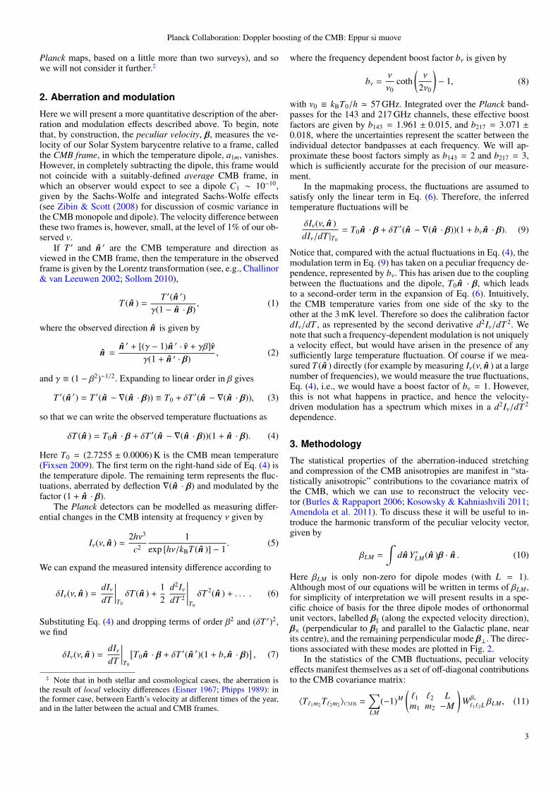
where the frequency dependent boost factor bν is given by

bν =ν

ν0coth

(ν

2ν0

)− 1, (8)

with ν0 ≡ kBT0/h ' 57 GHz. Integrated over the Planck band-passes for the 143 and 217 GHz channels, these effective boostfactors are given by b143 = 1.961 ± 0.015, and b217 = 3.071 ±0.018, where the uncertainties represent the scatter between theindividual detector bandpasses at each frequency. We will ap-proximate these boost factors simply as b143 = 2 and b217 = 3,which is sufficiently accurate for the precision of our measure-ment.

In the mapmaking process, the fluctuations are assumed tosatisfy only the linear term in Eq. (6). Therefore, the inferredtemperature fluctuations will be

δIν(ν, n )dIν/dT |T0

= T0 n · β + δT ′(n − ∇(n · β))(1 + bν n · β). (9)

Notice that, compared with the actual fluctuations in Eq. (4), themodulation term in Eq. (9) has taken on a peculiar frequency de-pendence, represented by bν. This has arisen due to the couplingbetween the fluctuations and the dipole, T0 n · β, which leadsto a second-order term in the expansion of Eq. (6). Intuitively,the CMB temperature varies from one side of the sky to theother at the 3 mK level. Therefore so does the calibration factordIν/dT , as represented by the second derivative d2Iν/dT 2. Wenote that such a frequency-dependent modulation is not uniquelya velocity effect, but would have arisen in the presence of anysufficiently large temperature fluctuation. Of course if we mea-sured T (n ) directly (for example by measuring Iν(ν, n ) at a largenumber of frequencies), we would measure the true fluctuations,Eq. (4), i.e., we would have a boost factor of bν = 1. However,this is not what happens in practice, and hence the velocity-driven modulation has a spectrum which mixes in a d2Iν/dT 2

dependence.

3. Methodology

The statistical properties of the aberration-induced stretchingand compression of the CMB anisotropies are manifest in “sta-tistically anisotropic” contributions to the covariance matrix ofthe CMB, which we can use to reconstruct the velocity vec-tor (Burles & Rappaport 2006; Kosowsky & Kahniashvili 2011;Amendola et al. 2011). To discuss these it will be useful to in-troduce the harmonic transform of the peculiar velocity vector,given by

βLM =

∫dn Y∗LM(n )β · n . (10)

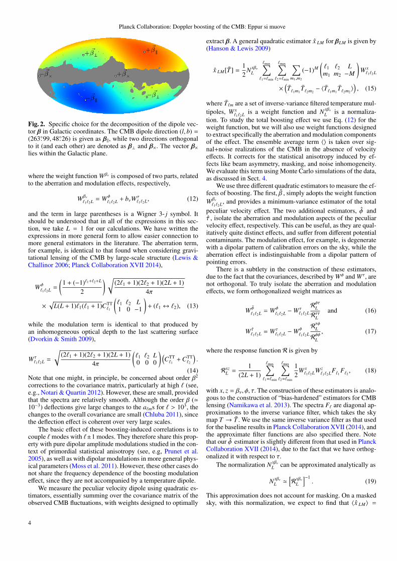
Here βLM is only non-zero for dipole modes (with L = 1).Although most of our equations will be written in terms of βLM ,for simplicity of interpretation we will present results in a spe-cific choice of basis for the three dipole modes of orthonormalunit vectors, labelled β‖ (along the expected velocity direction),β× (perpendicular to β‖ and parallel to the Galactic plane, nearits centre), and the remaining perpendicular mode β⊥. The direc-tions associated with these modes are plotted in Fig. 2.

In the statistics of the CMB fluctuations, peculiar velocityeffects manifest themselves as a set of off-diagonal contributionsto the CMB covariance matrix:

〈T`1m2 T`2m2〉cmb =∑LM

(−1)M(`1 `2 Lm1 m2 −M

)Wβν`1`2L βLM , (11)

3

Planck Collaboration: Doppler boosting of the CMB: Eppur si muove

+ ~β

−~β − ~β

+ ~β

+ ~β×− ~β×

Fig. 2. Specific choice for the decomposition of the dipole vec-tor β in Galactic coordinates. The CMB dipole direction (l, b) =(263.◦99, 48.◦26) is given as β‖, while two directions orthogonalto it (and each other) are denoted as β⊥ and β×. The vector β×lies within the Galactic plane.

where the weight function Wβν is composed of two parts, relatedto the aberration and modulation effects, respectively,

Wβν`1`2L = Wφ

`1`2L + bνWτ`1`2L, (12)

and the term in large parentheses is a Wigner 3- j symbol. Itshould be understood that in all of the expressions in this sec-tion, we take L = 1 for our calculations. We have written theexpressions in more general form to allow easier connection tomore general estimators in the literature. The aberration term,for example, is identical to that found when considering gravi-tational lensing of the CMB by large-scale structure (Lewis &Challinor 2006; Planck Collaboration XVII 2014),

Wφ`1`2L =

(1 + (−1)`1+`2+L

2

) √(2`1 + 1)(2`2 + 1)(2L + 1)

4π

×√

L(L + 1)`1(`1 + 1)CTT`1

(`1 `2 L1 0 −1

)+ (`1 ↔ `2), (13)

while the modulation term is identical to that produced byan inhomogeneous optical depth to the last scattering surface(Dvorkin & Smith 2009),

Wτ`1`2L =

√(2`1 + 1)(2`2 + 1)(2L + 1)

4π

(`1 `2 L0 0 0

) (CTT`1

+ CTT`2

).

(14)Note that one might, in principle, be concerned about order β2

corrections to the covariance matrix, particularly at high ` (see,e.g., Notari & Quartin 2012). However, these are small, providedthat the spectra are relatively smooth. Although the order β ('10−3) deflections give large changes to the a`ms for ` > 103, thechanges to the overall covariance are small (Chluba 2011), sincethe deflection effect is coherent over very large scales.

The basic effect of these boosting-induced correlations is tocouple ` modes with `±1 modes. They therefore share this prop-erty with pure dipolar amplitude modulations studied in the con-text of primordial statistical anisotropy (see, e.g, Prunet et al.2005), as well as with dipolar modulations in more general phys-ical parameters (Moss et al. 2011). However, these other cases donot share the frequency dependence of the boosting modulationeffect, since they are not accompanied by a temperature dipole.

We measure the peculiar velocity dipole using quadratic es-timators, essentially summing over the covariance matrix of theobserved CMB fluctuations, with weights designed to optimally

extract β. A general quadratic estimator x LM for βLM is given by(Hanson & Lewis 2009)

x LM[T ] =12

N xβνL

`max∑`1=`min

`max∑`2=`min

∑m1,m2

(−1)M(`1 `2 Lm1 m2 −M

)W x`1`2L

×(T`1m1

T`2m2− 〈T`1m1

T`2m2〉), (15)

where T`m are a set of inverse-variance filtered temperature mul-tipoles, W x

`1`2L is a weight function and N xβνL is a normaliza-

tion. To study the total boosting effect we use Eq. (12) for theweight function, but we will also use weight functions designedto extract specifically the aberration and modulation componentsof the effect. The ensemble average term 〈〉 is taken over sig-nal+noise realizations of the CMB in the absence of velocityeffects. It corrects for the statistical anisotropy induced by ef-fects like beam asymmetry, masking, and noise inhomogeneity.We evaluate this term using Monte Carlo simulations of the data,as discussed in Sect. 4.

We use three different quadratic estimators to measure the ef-fects of boosting. The first, β , simply adopts the weight functionWβν`1`2L, and provides a minimum-variance estimator of the total

peculiar velocity effect. The two additional estimators, φ andτ , isolate the aberration and modulation aspects of the peculiarvelocity effect, respectively. This can be useful, as they are qual-itatively quite distinct effects, and suffer from different potentialcontaminants. The modulation effect, for example, is degeneratewith a dipolar pattern of calibration errors on the sky, while theaberration effect is indistinguishable from a dipolar pattern ofpointing errors.

There is a subtlety in the construction of these estimators,due to the fact that the covariances, described by Wφ and Wτ, arenot orthogonal. To truly isolate the aberration and modulationeffects, we form orthogonalized weight matrices as

W φ`1`2L = Wφ

`1`2L −Wτ`1`2L

RφτL

RττLand (16)

W τ`1`2L = Wτ

`1`2L −Wφ`1`2L

RτφL

RφφL

, (17)

where the response function R is given by

RxzL =

1(2L + 1)

`max∑`1=`min

`max∑`2=`min

12

W x`1`2LWz

`1`2LF`1F`2

, (18)

with x, z = βν, φ, τ. The construction of these estimators is analo-gous to the construction of “bias-hardened” estimators for CMBlensing (Namikawa et al. 2013). The spectra F` are diagonal ap-proximations to the inverse variance filter, which takes the skymap T → T . We use the same inverse variance filter as that usedfor the baseline results in Planck Collaboration XVII (2014), andthe approximate filter functions are also specified there. Notethat our φ estimator is slightly different from that used in PlanckCollaboration XVII (2014), due to the fact that we have orthog-onalized it with respect to τ.

The normalization N xβνL can be approximated analytically as

N xβνL '

[R

xβνL

]−1. (19)

This approximation does not account for masking. On a maskedsky, with this normalization, we expect to find that 〈x LM〉 =

4

Planck Collaboration: Doppler boosting of the CMB: Eppur si muove

fLM, sky βLM , where

fLM, sky =

∫dn Y∗LM(n )M(n )β‖ · n . (20)

Here M(n ) is the sky mask used in our analysis. For the fiducialsky mask we use (plotted in Fig. 2, and which leaves approx-imately 70% of the sky unmasked), taking the dot product off1M, sky with our three basis vectors we find that f‖, sky = 0.82,f⊥, sky = 0.17, and f×, sky = −0.04. The large effective sky frac-tion for the β‖ direction reflects the fact that the peaks of theexpected velocity dipole are untouched by the mask, while thesmall values of fsky for the other components reflects that factthat the masking procedure does not leak a large amount of thedipole signal in the β‖ direction into other modes.

4. Data and simulations

Given the frequency-dependent nature of the velocity effects weare searching for (at least for the τ component), we will focusfor the most part on estimates of β obtained from individual fre-quency maps, although in Sect. 6 we will also discuss the analy-sis of component-separated maps obtained from combinations ofthe entire Planck frequency range. Our analysis procedure is es-sentially identical to that of Planck Collaboration XVII (2014),and so we only provide a brief review of it here. We use the143 and 217 GHz Planck maps, which contain the majority ofthe available CMB signal probed by Planck at the high mul-tipoles required to observe the velocity effects. The 143 GHzmap has a noise level that is reasonably well approximated by45 µK arcmin white noise, while the 217 GHz map has approxi-mately twice as much noise power, with a level of 60 µK arcmin.The beam at 143 GHz is approximately 7′ FWHM, while the217 GHz beam is 5′ FWHM. This increased angular resolu-tion, as well as the larger size of the τ-type velocity signal athigher frequency, makes 217 GHz slightly more powerful than143 GHz for detecting velocity effects (the HFI 100 GHz and LFI70 GHz channels would offer very little additional constrainingpower). At these noise levels, for 70% sky coverage we Fisher-forecast a 20% measurement of the component β‖ at 217 GHz(or, alternatively, a 5σ detection) or a 25% measurement ofβ‖ at 143 GHz, consistent with the estimates of Kosowsky &Kahniashvili (2011) and Amendola et al. (2011). As we willsee, our actual statistical error bars determined from simulationsagree well with these expectations.

The Planck maps are generated at HEALPix (Gorski et al.2005)§ Nside = 2048. In the process of mapmaking, time-domainobservations are binned into pixels. This effectively generates apointing error, given by the distance between the pixel centre towhich each observation is assigned and the true pointing direc-tion at that time. The pixels at Nside = 2048 have a typical dimen-sion of 1.′7. As this is comparable to the size of the aberrationeffect we are looking for, this is a potential source of concern.However, as discussed in Planck Collaboration XVII (2014), thebeam-convolved CMB is sufficiently smooth on these scales thatit is well approximated as a gradient across each pixel, and theerrors accordingly average down with the distribution of hits ineach pixel. For the frequency maps that we use, the rms pix-elization error is on the order of 0.′1, and not coherent over thelarge dipole scales which we are interested in, and so we neglectpixelization effects in our measurement.

We will use several data combinations to measure β. Thequadratic estimator of Eq. (15) has two input “legs,” i.e., the `1m1

§ http://healpix.jpl.nasa.gov

and `2m2 terms. Starting from the 143 and 217 GHz maps, thereare three distinct ways we may source these legs: (1) both legsuse either the individually filtered 143 GHz or 217 GHz maps,which we refer to as 143 × 143 and 217 × 217, respectively; (2)we can use 143 GHz for one leg, and 217 GHz for the other, re-ferred to as 143 × 217; and (3) we can combine both 143 and217 GHz data in our inverse-variance filtering procedure intoa single minimum-variance map, which is then fed into bothlegs of the quadratic estimator. We refer to this final combina-tion schematically as “143+217.” Combinations (2) and (3) mix143 and 217 GHz data. When constructing the weight functionof Eq. (12) for these combinations we use an effective bν = 2.5.Note that this effective bν is only used to determine the weightfunction of the quadratic estimator; errors in the approximationwill make our estimator suboptimal, but will not bias our results.To construct the T , which are the inputs for these quadratic esti-mators, we use the filtering described in Appendix A of PlanckCollaboration XVII (2014), which optimally accounts for theGalactic and point source masking (although not for the inho-mogeneity of the instrumental noise level). This filter inverse-variance weights the CMB fluctuations, and also projects out the857 GHz Planck map as a dust template.

To characterize our estimator and to compute the mean-fieldterm of Eq. (15), we use a large set of Monte Carlo simulations.These are generated following the same procedure as those de-scribed in Planck Collaboration XVII (2014); they incorporatethe asymmetry of the instrumental beam, gravitational lensingeffects, and realistic noise realizations from the FFP6 simula-tion set described in Planck Collaboration I (2014) and PlanckCollaboration (2013). There is one missing aspect of these simu-lations which we discuss briefly here: due to an oversight in theirpreparation, the gravitational lensing component of our simula-tions only included lensing power for lensing modes on scalesL ≥ 2, which leads to a slight underestimation of our simulation-based error bars for the φ component of the velocity estima-tor. The lensing dipole power in the fiducial ΛCDM model isCφφ

1 ' 6 × 10−8, which represents an additional source of noisefor each mode of β, given by σφ,lens = 1.2 × 10−4, or aboutone tenth the size of the expected signal. The φ part of the es-timator contributes approximately 46% of the total β estimatorweight at 143 GHz, and 35% at 217 GHz. Our measurement er-rors without this lensing noise on an individual mode of β areσβ ' 2.5 × 10−4, while with lensing noise included we would

expect this to increase to√σ2β + (4/10)2σ2

φ,lens = 2.54 × 10−4.This is small enough that we have neglected it for these results(rather than include it by hand).

We generate simulations both with and without peculiar ve-locity effects, to determine the normalization of our estimator,which, as we will see, is reasonably consistent with the analyt-ical expectation discussed around Eq. (20). All of our main re-sults with frequency maps use 1000 simulations to determine theestimator mean field and variance, while the component separa-tion tests in Sect. 6 use 300 simulations.

5. Results

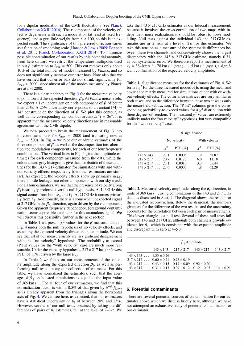
We present our results visually in Fig. 3, where we plot the to-tal measured dipole direction β as a function of the maximumtemperature multipole `max used as input to our quadratic esti-mators. We can see that all four of our 143/217 GHz based es-timators converge toward the expected dipole direction at high`max. At `max < 100, we recover the significantly preferred direc-tion of Hoftuft et al. (2009), which is identified when searching

5

Planck Collaboration: Doppler boosting of the CMB: Eppur si muove

for a dipolar modulation of the CMB fluctuations (see PlanckCollaboration XXIII 2014). The τ component of the velocity ef-fect is degenerate with such a modulation (at least at fixed fre-quency), and φ gets little weight from ` < 100, so this is an ex-pected result. The significance of this preferred direction variesas a function of smoothing scale (Hanson & Lewis 2009; Bennettet al. 2011; Planck Collaboration XXIII 2014). To minimizepossible contamination of our results by this potential anomaly,from here onward we restrict the temperature multipoles usedin our β estimation to `min = 500. This cut removes only about10% of the total number of modes measured by Planck, and sodoes not significantly increase our error bars. Note also that wehave verified that our error bars do not shrink significantly for`max > 2000, since almost all of the modes measured by Planckare at ` < 2000.

There is a clear tendency in Fig. 3 for the measured velocityto point toward the expected direction β‖. At Planck noise levels,we expect a 1σ uncertainty on each component of β of betterthan 25%. A 25% uncertainty corresponds to an arctan(1/4) =14◦ constraint on the direction of β. We plot this contour, aswell as the corresponding 2σ contour arctan(2/4) = 26◦. It isapparent that the measured velocity directions are in reasonableagreement with the CMB dipole.

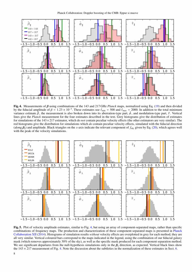
We now proceed to break the measurement of Fig. 3 intoits constituent parts for `max = 2000 (and truncating now at`min = 500). In Fig. 4 we plot our quadratic estimates of thethree components of β, as well as the decomposition into aberra-tion and modulation components, for each of our four frequencycombinations. The vertical lines in Fig. 4 give the amplitude es-timates for each component measured from the data, while thecoloured and grey histograms give the distribution of these quan-tities for the 143 × 217 estimator, for simulations with and with-out velocity effects, respectively (the other estimators are simi-lar). As expected, the velocity effects show up primarily in β‖;there is little leakage into other components with our sky mask.For all four estimators, we see that the presence of velocity alongβ‖ is strongly preferred over the null hypothesis. At 143 GHz thissignal comes from both φ ‖ and τ ‖. At 217 GHz it comes primar-ily from τ ‖. Additionally, there is a somewhat unexpected signalat 217 GHz in the β× direction, again driven by the τ component.Given the apparent frequency dependence, foreground contami-nation seems a possible candidate for this anomalous signal. Wewill discuss this possibility further in the next section.

In Table 1 we present χ2 values for the β measurements ofFig. 4 under both the null hypothesis of no velocity effects, andassuming the expected velocity direction and amplitude. We cansee that all of our measurements are in significant disagreementwith the “no velocity” hypothesis. The probability-to-exceed(PTE) values for the “with velocity” case are much more rea-sonable. Under the velocity hypothesis, 217×217 has the lowestPTE, of 11%, driven by the large β ×.

In Table 2 we focus on our measurements of the veloc-ity amplitude along the expected direction β‖, as well as per-forming null tests among our collection of estimates. For thistable, we have normalized the estimators, such that the aver-age of β ‖ on boosted simulations is equal to the input valueof 369 km s−1. For all four of our estimators, we find that thisnormalization factor is within 0.5% of that given by N xβν f‖,sky,as is already apparent from the triangles along the horizontalaxis of Fig. 4. We can see here, as expected, that our estimatorshave a statistical uncertainty on β‖ of between 20% and 25%.However, several of our null tests, obtained by taking the dif-ferences of pairs of β‖ estimates, fail at the level of 2–3σ. We

take the 143 × 217 GHz estimator as our fiducial measurement;because it involves the cross-correlation of two maps with in-dependent noise realizations it should be robust to noise mod-elling. Null tests against the individual 143 and 217 GHz es-timates are in tension at a level of 2σ for this estimator. Wetake this tension as a measure of the systematic differences be-tween these two channels, and conservatively choose the largestdiscrepancy with the 143 × 217 GHz estimate, namely 0.31,as our systematic error. We therefore report a measurement ofv ‖ = 384 km s−1 ± 78 km s−1 (stat.)± 115 km s−1 (syst.), a signif-icant confirmation of the expected velocity amplitude.

Table 1. Significance measures for the β estimates of Fig. 4. Weform a χ2 for the three measured modes of β, using the mean andcovariance matrix measured for simulations either with or with-out velocity effects. The covariance matrices are very similar inboth cases, and so the difference between these two cases is onlythe mean-field subtraction. The “PTE” columns give the corre-sponding probability-to-exceed values for a χ2 distribution withthree degrees of freedom. The measured χ2 values are extremelyunlikely under the “no velocity” hypothesis, but very compatiblefor the “with velocity” case.

β significance

No velocity With velocity

χ2 PTE [%] χ2 PTE [%]

143 × 143 . . . 27.1 0.0005 1.9 58.87217 × 217 . . . 20.7 0.0123 6.0 11.18143 + 217 . . . 25.1 0.0015 3.3 35.44143 × 217 . . . 27.6 0.0005 1.8 62.29

Table 2. Measured velocity amplitudes along the β‖ direction, inunits of 369 km s−1, using combinations of the 143 and 217 GHzdata, as discussed in Sect. 4. The diagonal shows the results forthe indicated reconstruction. Below the diagonal, the numbersgiven are for the difference of the two results, and the uncertaintyaccounts for the correlation between each pair of measurements.This lower triangle is a null test. Several of these null tests failbetween 143 and 217 GHz, although both channels provide ev-idence for β‖, which is consistent with the expected amplitudeand discrepant with zero at 4–5σ.

β ‖ Amplitude

143 × 143 217 × 217 143 + 217 143 × 217

143 × 143 . . . 1.35 ± 0.26 2.10 ± 0.41 2.27 ± 0.44 2.39 ± 0.46217 × 217 . . . 0.60 ± 0.21 0.75 ± 0.19 1.67 ± 0.38 1.79 ± 0.38143 + 217 . . . 0.43 ± 0.15 −0.17 ± 0.09 0.92 ± 0.20 1.96 ± 0.40143 × 217 . . . 0.31 ± 0.13 −0.29 ± 0.12 −0.12 ± 0.07 1.04 ± 0.21

6. Potential contaminants

There are several potential sources of contamination for our es-timates above which we discuss briefly here, although we havenot attempted an exhaustive study of potential contaminants forour estimator.

6

Planck Collaboration: Doppler boosting of the CMB: Eppur si muove

100 2000lmax

+ ~β

−~β

+ ~β

− ~β

+ ~β×− ~β×

Fig. 3. Measured dipole direction β in Galactic coordinates as a function of the maximum temperature multipole used in theanalysis, `max. We plot the results for the four data combinations discussed in Sect. 4: 143× 143 (H symbol); 217× 217 (N symbol);143 × 217 (× symbol); and 143 + 217 (+ symbol). The CMB dipole direction β‖ has been highlighted with 14◦ and 26◦ radiuscircles, which correspond roughly to our expected uncertainty on the dipole direction. The black cross in the lower hemisphere isthe modulation dipole anomaly direction found for WMAP at `max = 64 in Hoftuft et al. (2009), and which is discussed further inPlanck Collaboration XXIII (2014). Note that all four estimators are significantly correlated with one another, even the 143 × 143and 217 × 217 results, which are based on maps with independent noise realizations. This is because a significant portion of thedipole measurement uncertainty is from sample variance of the CMB fluctuations, which is common between channels.

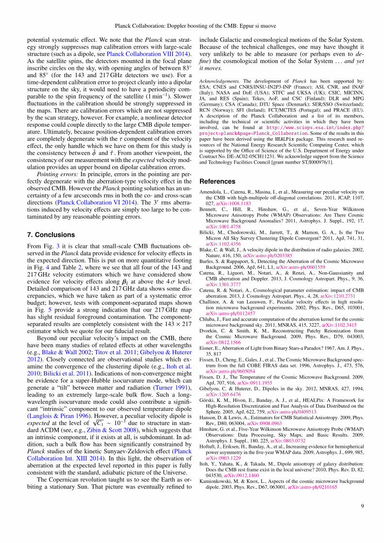
Galactic Foregrounds: Given the simplicity of the fore-ground correction we have used (consisting only of masking thesky and projecting out the Planck 857 GHz map as a crude dusttemplate), foreground contamination is a clear source of con-cern. The frequency dependence of the large β× signal seen at217 GHz, but not at 143 GHz, seems potentially indicative offoreground contamination, as the Galactic dust power is approx-imately 10 times larger at 217 than at 143 GHz. To test the pos-sible magnitude of residual foregrounds, we apply our veloc-ity estimators to the four component-separated CMB maps ofPlanck Collaboration XII (2014), i.e., NILC, SMICA, SEVEM, andCOMMANDER-RULER. Each of these methods combines the full setof nine Planck frequency maps from 30 to 857 GHz to obtain abest-estimate CMB map. To characterize the scatter and meanfield of each method’s map we use the set of common simula-tions which each method has been applied to. These simulationsinclude the effect of the aberration part of the velocity dipole,although not the frequency-dependent modulation part. For thisreason, it is difficult to accurately assess the normalization of ourestimators when applied to these maps, particularly as they canmix 143 and 217 GHz as a function of scale, and the modulationpart is frequency dependent. We can, however, study them at aqualitative level. The results of this analysis are shown in Fig. 5.

To construct our β estimator for the component-separated mapswe have used bν = 2.5, assuming that they contain roughly equalcontributions from 143 and 217 GHz. Note that, because the sim-ulations used to determine the mean fields of the component-separated map included the aberration part of the velocity effect,it will be absorbed into the mean field if uncorrected. Becausethe aberration contribution is frequency independent (so thereare no issues with how the different CMB channels are mixed),and given the good agreement between our analytical normaliza-tion and that measured using simulations for the frequency maps,when generating Fig. 5 we have subtracted the expected velocitycontribution from the mean field analytically. We see generallygood agreement with the 143 × 217 estimate on which we havebased our measurement of the previous section; there are no ob-vious discrepancies with our measurements in the β‖ direction,although there is a somewhat large scatter between methods forφ ‖. In the β× direction the component-separated map estimatesagree well with the 143 × 217 estimator, and do not show thesignificant power seen for 217 × 217, suggesting that the largepower that we see there may indeed be foreground in origin.

Calibration errors: Position-dependent calibration errors inour sky maps are completely degenerate with modulation-typeeffects (at fixed frequency), and so are very worrisome as a

7

Planck Collaboration: Doppler boosting of the CMB: Eppur si muove

1.5 1.0 0.5 0.0 0.5 1.0 1.5

β

143× 143

217× 217

143 + 217

143× 217

1.5 1.0 0.5 0.0 0.5 1.0 1.5

φ

1.5 1.0 0.5 0.0 0.5 1.0 1.5

τ

1.5 1.0 0.5 0.0 0.5 1.0 1.5

β

1.5 1.0 0.5 0.0 0.5 1.0 1.5

φ

1.5 1.0 0.5 0.0 0.5 1.0 1.5

τ

1.5 1.0 0.5 0.0 0.5 1.0 1.5

β×

1.5 1.0 0.5 0.0 0.5 1.0 1.5

φ×

1.5 1.0 0.5 0.0 0.5 1.0 1.5

τ×

Fig. 4. Measurements of β using combinations of the 143 and 217 GHz Planck maps, normalized using Eq. (19) and then dividedby the fiducial amplitude of β = 1.23 × 10−3. These estimates use `min = 500 and `max = 2000. In addition to the total minimumvariance estimate β , the measurement is also broken down into its aberration-type part, φ , and modulation-type part, τ . Verticallines give the Planck measurement for the four estimates described in the text. Grey histograms give the distribution of estimatesfor simulations of the 143×217 estimator, which do not contain peculiar velocity effects (the other estimators are very similar). Thered histograms give the distribution for simulations which do contain peculiar velocity effects, simulated with the fiducial direction(along β‖) and amplitude. Black triangles on the x-axis indicate the relevant component of fsky given by Eq. (20), which agrees wellwith the peak of the velocity simulations.

1.5 1.0 0.5 0.0 0.5 1.0 1.5

β

NILC

SMICA

SEVEM

RULER

1.5 1.0 0.5 0.0 0.5 1.0 1.5

φ

1.5 1.0 0.5 0.0 0.5 1.0 1.5

τ

1.5 1.0 0.5 0.0 0.5 1.0 1.5

β

1.5 1.0 0.5 0.0 0.5 1.0 1.5

φ

1.5 1.0 0.5 0.0 0.5 1.0 1.5

τ

1.5 1.0 0.5 0.0 0.5 1.0 1.5

β×

1.5 1.0 0.5 0.0 0.5 1.0 1.5

φ×

1.5 1.0 0.5 0.0 0.5 1.0 1.5

τ×

Fig. 5. Plot of velocity amplitude estimates, similar to Fig. 4, but using an array of component-separated maps, rather than specificcombinations of frequency maps. The production and characterization of these component-separated maps is presented in PlanckCollaboration XII (2014). Histograms of simulation results without velocity effects are overplotted in grey for each method; they areall very similar. Vertical coloured bars correspond to the maps indicated in the legend, using the combination of our fiducial galaxymask (which removes approximately 30% of the sky), as well as the specific mask produced for each component separation method.We see significant departures from the null-hypothesis simulations only in the β‖ direction, as expected. Vertical black lines showthe 143 × 217 measurement of Fig. 4. Note the discussion about the subtleties in the normalization of these estimates in Sect. 6.

8

Planck Collaboration: Doppler boosting of the CMB: Eppur si muove

potential systematic effect. We note that the Planck scan strat-egy strongly suppresses map calibration errors with large-scalestructure (such as a dipole, see Planck Collaboration VIII 2014).As the satellite spins, the detectors mounted in the focal planeinscribe circles on the sky, with opening angles of between 83◦and 85◦ (for the 143 and 217 GHz detectors we use). For atime-dependent calibration error to project cleanly into a dipolarstructure on the sky, it would need to have a periodicity com-parable to the spin frequency of the satellite (1 min−1). Slowerfluctuations in the calibration should be strongly suppressed inthe maps. There are calibration errors which are not suppressedby the scan strategy, however. For example, a nonlinear detectorresponse could couple directly to the large CMB dipole temper-ature. Ultimately, because position-dependent calibration errorsare completely degenerate with the τ component of the velocityeffect, the only handle which we have on them for this study isthe consistency between φ and τ . From another viewpoint, theconsistency of our measurement with the expected velocity mod-ulation provides an upper bound on dipolar calibration errors.

Pointing errors: In principle, errors in the pointing are per-fectly degenerate with the aberration-type velocity effect in theobserved CMB. However the Planck pointing solution has an un-certainty of a few arcseconds rms in both the co- and cross-scandirections (Planck Collaboration VI 2014). The 3′ rms aberra-tions induced by velocity effects are simply too large to be con-taminated by any reasonable pointing errors.

7. Conclusions

From Fig. 3 it is clear that small-scale CMB fluctuations ob-served in the Planck data provide evidence for velocity effects inthe expected direction. This is put on more quantitative footingin Fig. 4 and Table 2, where we see that all four of the 143 and217 GHz velocity estimators which we have considered showevidence for velocity effects along β‖ at above the 4σ level.Detailed comparison of 143 and 217 GHz data shows some dis-crepancies, which we have taken as part of a systematic errorbudget; however, tests with component-separated maps shownin Fig. 5 provide a strong indication that our 217 GHz maphas slight residual foreground contamination. The component-separated results are completely consistent with the 143 × 217estimator which we quote for our fiducial result.

Beyond our peculiar velocity’s impact on the CMB, therehave been many studies of related effects at other wavelengths(e.g., Blake & Wall 2002; Titov et al. 2011; Gibelyou & Huterer2012). Closely connected are observational studies which ex-amine the convergence of the clustering dipole (e.g., Itoh et al.2010; Bilicki et al. 2011). Indications of non-convergence mightbe evidence for a super-Hubble isocurvature mode, which cangenerate a “tilt” between matter and radiation (Turner 1991),leading to an extremely large-scale bulk flow. Such a long-wavelength isocurvature mode could also contribute a signifi-cant “intrinsic” component to our observed temperature dipole(Langlois & Piran 1996). However, a peculiar velocity dipole isexpected at the level of

√C1 ∼ 10−3 due to structure in stan-

dard ΛCDM (see, e.g., Zibin & Scott 2008), which suggests thatan intrinsic component, if it exists at all, is subdominant. In ad-dition, such a bulk flow has been significantly constrained byPlanck studies of the kinetic Sunyaev-Zeldovich effect (PlanckCollaboration Int. XIII 2014). In this light, the observation ofaberration at the expected level reported in this paper is fullyconsistent with the standard, adiabatic picture of the Universe.

The Copernican revolution taught us to see the Earth as or-biting a stationary Sun. That picture was eventually refined to

include Galactic and cosmological motions of the Solar System.Because of the technical challenges, one may have thought itvery unlikely to be able to measure (or perhaps even to de-fine) the cosmological motion of the Solar System . . . and yetit moves.

Acknowledgements. The development of Planck has been supported by:ESA; CNES and CNRS/INSU-IN2P3-INP (France); ASI, CNR, and INAF(Italy); NASA and DoE (USA); STFC and UKSA (UK); CSIC, MICINN,JA, and RES (Spain); Tekes, AoF, and CSC (Finland); DLR and MPG(Germany); CSA (Canada); DTU Space (Denmark); SER/SSO (Switzerland);RCN (Norway); SFI (Ireland); FCT/MCTES (Portugal); and PRACE (EU).A description of the Planck Collaboration and a list of its members,including the technical or scientific activities in which they have beeninvolved, can be found at http://www.sciops.esa.int/index.php?project=planck&page=Planck_Collaboration. Some of the results in thispaper have been derived using the HEALPix package. This research used re-sources of the National Energy Research Scientific Computing Center, whichis supported by the Office of Science of the U.S. Department of Energy underContract No. DE-AC02-05CH11231. We acknowledge support from the Scienceand Technology Facilities Council [grant number ST/I000976/1].

ReferencesAmendola, L., Catena, R., Masina, I., et al., Measuring our peculiar velocity on

the CMB with high-multipole off-diagonal correlations. 2011, JCAP, 1107,027, arXiv:1008.1183

Bennett, C., Hill, R., Hinshaw, G., et al., Seven-Year WilkinsonMicrowave Anisotropy Probe (WMAP) Observations: Are There CosmicMicrowave Background Anomalies? 2011, Astrophys. J. Suppl., 192, 17,arXiv:1001.4758

Bilicki, M., Chodorowski, M., Jarrett, T., & Mamon, G. A., Is the TwoMicron All Sky Survey Clustering Dipole Convergent? 2011, ApJ, 741, 31,arXiv:1102.4356

Blake, C. & Wall, J., A velocity dipole in the distribution of radio galaxies. 2002,Nature, 416, 150, arXiv:astro-ph/0203385

Burles, S. & Rappaport, S., Detecting the Aberration of the Cosmic MicrowaveBackground. 2006, ApJ, 641, L1, arXiv:astro-ph/0601559

Catena, R., Liguori, M., Notari, A., & Renzi, A., Non-Gaussianity andCMB aberration and Doppler. 2013, J. Cosmology Astropart. Phys., 9, 36,arXiv:1301.3777

Catena, R. & Notari, A., Cosmological parameter estimation: impact of CMBaberration. 2013, J. Cosmology Astropart. Phys., 4, 28, arXiv:1210.2731

Challinor, A. & van Leeuwen, F., Peculiar velocity effects in high resolu-tion microwave background experiments. 2002, Phys. Rev., D65, 103001,arXiv:astro-ph/0112457

Chluba, J., Fast and accurate computation of the aberration kernel for the cosmicmicrowave background sky. 2011, MNRAS, 415, 3227, arXiv:1102.3415

Dvorkin, C. & Smith, K. M., Reconstructing Patchy Reionization fromthe Cosmic Microwave Background. 2009, Phys. Rev., D79, 043003,arXiv:0812.1566

Eisner, E., Aberration of Light from Binary Stars-a Paradox? 1967, Am. J. Phys.,35, 817

Fixsen, D., Cheng, E., Gales, J., et al., The Cosmic Microwave Background spec-trum from the full COBE FIRAS data set. 1996, Astrophys. J., 473, 576,arXiv:astro-ph/9605054

Fixsen, D. J., The Temperature of the Cosmic Microwave Background. 2009,ApJ, 707, 916, arXiv:0911.1955

Gibelyou, C. & Huterer, D., Dipoles in the sky. 2012, MNRAS, 427, 1994,arXiv:1205.6476

Gorski, K. M., Hivon, E., Banday, A. J., et al., HEALPix: A Framework forHigh-Resolution Discretization and Fast Analysis of Data Distributed on theSphere. 2005, ApJ, 622, 759, arXiv:astro-ph/0409513

Hanson, D. & Lewis, A., Estimators for CMB Statistical Anisotropy. 2009, Phys.Rev., D80, 063004, arXiv:0908.0963

Hinshaw, G. et al., Five-Year Wilkinson Microwave Anisotropy Probe (WMAP)Observations: Data Processing, Sky Maps, and Basic Results. 2009,Astrophys. J. Suppl., 180, 225, arXiv:0803.0732

Hoftuft, J., Eriksen, H., Banday, A., et al., Increasing evidence for hemisphericalpower asymmetry in the five-year WMAP data. 2009, Astrophys. J., 699, 985,arXiv:0903.1229

Itoh, Y., Yahata, K., & Takada, M., Dipole anisotropy of galaxy distribution:Does the CMB rest frame exist in the local universe? 2010, Phys. Rev. D, 82,043530, arXiv:0912.1460

Kamionkowski, M. & Knox, L., Aspects of the cosmic microwave backgrounddipole. 2003, Phys. Rev., D67, 063001, arXiv:astro-ph/0210165

9

Planck Collaboration: Doppler boosting of the CMB: Eppur si muove

Kogut, A., Lineweaver, C., Smoot, G. F., et al., Dipole anisotropy in theCOBE DMR first year sky maps. 1993, Astrophys. J., 419, 1, arXiv:astro-ph/9312056

Kosowsky, A. & Kahniashvili, T., The Signature of Proper Motion in theMicrowave Sky. 2011, Phys. Rev. Lett., 106, 191301, arXiv:1007.4539

Langlois, D. & Piran, T., Cosmic microwave background dipole from an entropygradient. 1996, Phys. Rev. D, 53, 2908, arXiv:astro-ph/9507094

Lewis, A. & Challinor, A., Weak gravitational lensing of the cmb. 2006, Phys.Rept., 429, 1, arXiv:astro-ph/0601594

Moss, A., Scott, D., Zibin, J. P., & Battye, R., Tilted physics: A cosmologicallydipole-modulated sky. 2011, Phys. Rev. D, 84, 023014, arXiv:1011.2990

Namikawa, T., Hanson, D., & Takahashi, R., Bias-hardened CMB lensing. 2013,MNRAS, arXiv:1209.0091

Notari, A. & Quartin, M., Measuring our Peculiar Velocity by ’Pre-deboosting’the CMB. 2012, JCAP, 1202, 026, arXiv:1112.1400

Pereira, T. S., Yoho, A., Stuke, M., & Starkman, G. D., Effects of a Cut,Lorentz-Boosted sky on the Angular Power Spectrum. 2010, ArXiv e-prints,arXiv:1009.4937

Phipps, T. E., Relativity and aberration. 1989, Am. J. Phys., 57, 549Planck Collaboration. 2013, The Explanatory Supplement to the Planck 2013 re-

sults, http://www.sciops.esa.int/wikiSI/planckpla/index.php?title=Main Page(ESA)

Planck Collaboration I, Planck 2013 results: Overview of Planck Products andScientific Results. 2014, A&A, 571, A1

Planck Collaboration VI, Planck 2013 results: High Frequency Instrument DataProcessing. 2014, A&A, 571, A6

Planck Collaboration VIII, Planck 2013 results: HFI calibration and Map-making. 2014, A&A, 571, A8

Planck Collaboration XII, Planck 2013 results: Component separation. 2014,A&A, 571, A12

Planck Collaboration XV, Planck 2013 results: CMB power spectra and likeli-hood. 2014, A&A, 571, A15

Planck Collaboration XVI, Planck 2013 results: Cosmological parameters. 2014,A&A, 571, A16

Planck Collaboration XVII, Planck 2013 results: Gravitational lensing by large-scale structure. 2014, A&A, 571, A17

Planck Collaboration XXIII, Planck 2013 results: Isotropy and statistics of theCMB. 2014, A&A, 571, A23

Planck Collaboration XXIV, Planck 2013 results: Constraints on primordial non-Gaussianity. 2014, A&A, 571, A24

Planck Collaboration Int. XIII, Planck intermediate results. XIII. Constraints onpeculiar velocities. 2014, A&A, 561, A97

Prunet, S., Uzan, J.-P., Bernardeau, F., & Brunier, T., Constraints on mode cou-plings and modulation of the CMB with WMAP data. 2005, Phys. Rev. D,71, 083508, arXiv:astro-ph/0406364

Sollom, I. 2010, PhD thesis, University of Cambridge, United KingdomTitov, O., Lambert, S. B., & Gontier, A.-M., VLBI measurement of the secular

aberration drift. 2011, A&A, 529, A91, arXiv:1009.3698Turner, M. S., Tilted Universe and other remnants of the preinflationary

Universe. 1991, Phys. Rev. D, 44, 3737Yoho, A., Copi, C. J., Starkman, G. D., & Pereira, T. S., Real Space Approach to

CMB deboosting. 2012, ArXiv e-prints, arXiv:1211.6756Zibin, J. P. & Scott, D., Gauging the cosmic microwave background. 2008,

Phys. Rev. D, 78, 123529, arXiv:0808.2047

1 APC, AstroParticule et Cosmologie, Universite Paris Diderot,CNRS/IN2P3, CEA/lrfu, Observatoire de Paris, Sorbonne ParisCite, 10, rue Alice Domon et Leonie Duquet, 75205 Paris Cedex13, France

2 Aalto University Metsahovi Radio Observatory and Dept of RadioScience and Engineering, P.O. Box 13000, FI-00076 AALTO,Finland

3 African Institute for Mathematical Sciences, 6-8 Melrose Road,Muizenberg, Cape Town, South Africa

4 Agenzia Spaziale Italiana Science Data Center, Via del Politecnicosnc, 00133, Roma, Italy

5 Agenzia Spaziale Italiana, Viale Liegi 26, Roma, Italy6 Astrophysics Group, Cavendish Laboratory, University of

Cambridge, J J Thomson Avenue, Cambridge CB3 0HE, U.K.7 Astrophysics & Cosmology Research Unit, School of Mathematics,

Statistics & Computer Science, University of KwaZulu-Natal,Westville Campus, Private Bag X54001, Durban 4000, SouthAfrica

8 CITA, University of Toronto, 60 St. George St., Toronto, ON M5S3H8, Canada

9 CNRS, IRAP, 9 Av. colonel Roche, BP 44346, F-31028 Toulousecedex 4, France

10 California Institute of Technology, Pasadena, California, U.S.A.11 Centre for Theoretical Cosmology, DAMTP, University of

Cambridge, Wilberforce Road, Cambridge CB3 0WA, U.K.12 Computational Cosmology Center, Lawrence Berkeley National

Laboratory, Berkeley, California, U.S.A.13 DSM/Irfu/SPP, CEA-Saclay, F-91191 Gif-sur-Yvette Cedex,

France14 DTU Space, National Space Institute, Technical University of

Denmark, Elektrovej 327, DK-2800 Kgs. Lyngby, Denmark15 Departement de Physique Theorique, Universite de Geneve, 24,

Quai E. Ansermet,1211 Geneve 4, Switzerland16 Departamento de Fısica Fundamental, Facultad de Ciencias,

Universidad de Salamanca, 37008 Salamanca, Spain17 Departamento de Fısica, Universidad de Oviedo, Avda. Calvo

Sotelo s/n, Oviedo, Spain18 Department of Astrophysics/IMAPP, Radboud University

Nijmegen, P.O. Box 9010, 6500 GL Nijmegen, The Netherlands19 Department of Electrical Engineering and Computer Sciences,

University of California, Berkeley, California, U.S.A.20 Department of Physics & Astronomy, University of British

Columbia, 6224 Agricultural Road, Vancouver, British Columbia,Canada

21 Department of Physics and Astronomy, Dana and David DornsifeCollege of Letter, Arts and Sciences, University of SouthernCalifornia, Los Angeles, CA 90089, U.S.A.

22 Department of Physics and Astronomy, University CollegeLondon, London WC1E 6BT, U.K.

23 Department of Physics and Astronomy, University of Sussex,Brighton BN1 9QH, U.K.

24 Department of Physics, Florida State University, Keen PhysicsBuilding, 77 Chieftan Way, Tallahassee, Florida, U.S.A.

25 Department of Physics, Gustaf Hallstromin katu 2a, University ofHelsinki, Helsinki, Finland

26 Department of Physics, Princeton University, Princeton, NewJersey, U.S.A.

27 Department of Physics, University of California, Berkeley,California, U.S.A.

28 Department of Physics, University of California, One ShieldsAvenue, Davis, California, U.S.A.

29 Department of Physics, University of California, Santa Barbara,California, U.S.A.

30 Department of Physics, University of Illinois atUrbana-Champaign, 1110 West Green Street, Urbana, Illinois,U.S.A.

31 Dipartimento di Fisica e Astronomia G. Galilei, Universita degliStudi di Padova, via Marzolo 8, 35131 Padova, Italy

32 Dipartimento di Fisica e Scienze della Terra, Universita di Ferrara,Via Saragat 1, 44122 Ferrara, Italy

33 Dipartimento di Fisica, Universita La Sapienza, P. le A. Moro 2,Roma, Italy

34 Dipartimento di Fisica, Universita degli Studi di Milano, ViaCeloria, 16, Milano, Italy

35 Dipartimento di Fisica, Universita degli Studi di Trieste, via A.Valerio 2, Trieste, Italy

36 Dipartimento di Fisica, Universita di Roma Tor Vergata, Via dellaRicerca Scientifica, 1, Roma, Italy

37 Discovery Center, Niels Bohr Institute, Blegdamsvej 17,Copenhagen, Denmark

38 Dpto. Astrofısica, Universidad de La Laguna (ULL), E-38206 LaLaguna, Tenerife, Spain

39 European Space Agency, ESAC, Planck Science Office, Caminobajo del Castillo, s/n, Urbanizacion Villafranca del Castillo,Villanueva de la Canada, Madrid, Spain

40 European Space Agency, ESTEC, Keplerlaan 1, 2201 AZNoordwijk, The Netherlands

41 Helsinki Institute of Physics, Gustaf Hallstromin katu 2, Universityof Helsinki, Helsinki, Finland

10

Planck Collaboration: Doppler boosting of the CMB: Eppur si muove

42 INAF - Osservatorio Astronomico di Padova, Vicolodell’Osservatorio 5, Padova, Italy

43 INAF - Osservatorio Astronomico di Roma, via di Frascati 33,Monte Porzio Catone, Italy

44 INAF - Osservatorio Astronomico di Trieste, Via G.B. Tiepolo 11,Trieste, Italy

45 INAF Istituto di Radioastronomia, Via P. Gobetti 101, 40129Bologna, Italy

46 INAF/IASF Bologna, Via Gobetti 101, Bologna, Italy47 INAF/IASF Milano, Via E. Bassini 15, Milano, Italy48 INFN, Sezione di Bologna, Via Irnerio 46, I-40126, Bologna, Italy49 INFN, Sezione di Roma 1, Universita di Roma Sapienza, Piazzale

Aldo Moro 2, 00185, Roma, Italy50 INFN/National Institute for Nuclear Physics, Via Valerio 2,

I-34127 Trieste, Italy51 IPAG: Institut de Planetologie et d’Astrophysique de Grenoble,

Universite Joseph Fourier, Grenoble 1 / CNRS-INSU, UMR 5274,Grenoble, F-38041, France

52 ISDC Data Centre for Astrophysics, University of Geneva, ch.d’Ecogia 16, Versoix, Switzerland

53 IUCAA, Post Bag 4, Ganeshkhind, Pune University Campus, Pune411 007, India

54 Imperial College London, Astrophysics group, BlackettLaboratory, Prince Consort Road, London, SW7 2AZ, U.K.

55 Infrared Processing and Analysis Center, California Institute ofTechnology, Pasadena, CA 91125, U.S.A.

56 Institut d’Astrophysique Spatiale, CNRS (UMR8617) UniversiteParis-Sud 11, Batiment 121, Orsay, France

57 Institut d’Astrophysique de Paris, CNRS (UMR7095), 98 bisBoulevard Arago, F-75014, Paris, France

58 Institute for Space Sciences, Bucharest-Magurale, Romania59 Institute of Astronomy and Astrophysics, Academia Sinica, Taipei,

Taiwan60 Institute of Astronomy, University of Cambridge, Madingley Road,

Cambridge CB3 0HA, U.K.61 Institute of Theoretical Astrophysics, University of Oslo, Blindern,

Oslo, Norway62 Instituto de Astrofısica de Canarias, C/Vıa Lactea s/n, La Laguna,

Tenerife, Spain63 Instituto de Fısica de Cantabria (CSIC-Universidad de Cantabria),

Avda. de los Castros s/n, Santander, Spain64 Jet Propulsion Laboratory, California Institute of Technology, 4800

Oak Grove Drive, Pasadena, California, U.S.A.65 Jodrell Bank Centre for Astrophysics, Alan Turing Building,

School of Physics and Astronomy, The University of Manchester,Oxford Road, Manchester, M13 9PL, U.K.

66 Kavli Institute for Cosmology Cambridge, Madingley Road,Cambridge, CB3 0HA, U.K.

67 LAL, Universite Paris-Sud, CNRS/IN2P3, Orsay, France68 LERMA, CNRS, Observatoire de Paris, 61 Avenue de

l’Observatoire, Paris, France69 Laboratoire AIM, IRFU/Service d’Astrophysique - CEA/DSM -

CNRS - Universite Paris Diderot, Bat. 709, CEA-Saclay, F-91191Gif-sur-Yvette Cedex, France

70 Laboratoire Traitement et Communication de l’Information, CNRS(UMR 5141) and Telecom ParisTech, 46 rue Barrault F-75634Paris Cedex 13, France

71 Laboratoire de Physique Subatomique et de Cosmologie,Universite Joseph Fourier Grenoble I, CNRS/IN2P3, InstitutNational Polytechnique de Grenoble, 53 rue des Martyrs, 38026Grenoble cedex, France

72 Laboratoire de Physique Theorique, Universite Paris-Sud 11 &CNRS, Batiment 210, 91405 Orsay, France

73 Lawrence Berkeley National Laboratory, Berkeley, California,U.S.A.

74 Max-Planck-Institut fur Astrophysik, Karl-Schwarzschild-Str. 1,85741 Garching, Germany

75 McGill Physics, Ernest Rutherford Physics Building, McGillUniversity, 3600 rue University, Montreal, QC, H3A 2T8, Canada

76 Niels Bohr Institute, Blegdamsvej 17, Copenhagen, Denmark

77 Observational Cosmology, Mail Stop 367-17, California Instituteof Technology, Pasadena, CA, 91125, U.S.A.

78 Optical Science Laboratory, University College London, GowerStreet, London, U.K.

79 SISSA, Astrophysics Sector, via Bonomea 265, 34136, Trieste,Italy

80 School of Physics and Astronomy, Cardiff University, QueensBuildings, The Parade, Cardiff, CF24 3AA, U.K.

81 School of Physics and Astronomy, University of Nottingham,Nottingham NG7 2RD, U.K.

82 Space Research Institute (IKI), Russian Academy of Sciences,Profsoyuznaya Str, 84/32, Moscow, 117997, Russia

83 Space Sciences Laboratory, University of California, Berkeley,California, U.S.A.

84 Stanford University, Dept of Physics, Varian Physics Bldg, 382 ViaPueblo Mall, Stanford, California, U.S.A.

85 Sub-Department of Astrophysics, University of Oxford, KebleRoad, Oxford OX1 3RH, U.K.

86 UPMC Univ Paris 06, UMR7095, 98 bis Boulevard Arago,F-75014, Paris, France

87 Universite de Toulouse, UPS-OMP, IRAP, F-31028 Toulouse cedex4, France

88 Universities Space Research Association, StratosphericObservatory for Infrared Astronomy, MS 232-11, Moffett Field,CA 94035, U.S.A.

89 Warsaw University Observatory, Aleje Ujazdowskie 4, 00-478Warszawa, Poland

11