Embed Size (px)
Citation preview

Journal of Physics Conference Series
OPEN ACCESS
Planar Doppler velocimetry using a Mach-Zehnderinterferometric filterTo cite this article Z-H Lu et al 2007 J Phys Conf Ser 85 012011
View the article online for updates and enhancements
You may also likeRelaxation Effects of the NegativeElectrode Tisnsb Using 119sn Moumlssbauerand 7li MAS NMR SpectroscopiesNicolas Dupre Karen Johnston AliDarwiche et al
-
Demonstration of Large Flatband VoltageShift by Designing Al2O3SiO2 LaminatedStructures with Multiple Interface DipoleLayersKoji Kita and Hironobu Kamata
-
(Invited) Characterization of InterfacialDipoles at Dielectric Stacks by XPSAnalysisSeiichi Miyazaki Akio Ohta and NobuyukiFujimura
-
This content was downloaded from IP address 1032375677 on 17022022 at 0951
Planar Doppler velocimetry using a Mach-Zehnder interferometric filter
Z-H Lu T O H Charrett H D Ford and R P Tatam
Engineering Photonics Group School of Engineering Cranfield University Cranfield Bedford MK43 OAL UK
Email rptatamcranfieldacuk
Abstract A planar Doppler velocimetry system to measure flow velocity fields is described The technique uses a Mach-Zehnder interferometric filter to convert Doppler frequency shifts into intensity variations The free spectral range of the filter can be selected by adjusting the optical path difference of the interferometer This allows the velocity measurement range sensitivity and resolution to be varied An experimental arrangement is described that incorporates a phase-locking system designed to stabilise the interferometric filter Two methods to process the interference fringe images are presented the first uses the shift of the fringe pattern to determine the Doppler shift along profiles The second provides a full-field measurement of the Doppler shift by determining the phase at each pixel in the images Results are presented here for measurements of velocity fields on a rotating disc with maximum velocities at the edge of plusmn70ms Measurements on a seeded air jet with a nozzle diameter of 20mm and an exit velocity of ~85ms are also presented
1 Introduction Planar Doppler Velocimetry (PDV) [1-5] also called Doppler Global Velocimetry (DGV) [67] measures the Doppler shift in the laser light scattered by particles embedded in a flow and thus determines the flow velocity using the Doppler equation (1)
c
)io(vv L Vsdotminus
=∆ˆˆ
(1)
where Lννν minus=∆ is the difference between the scattered light frequency ν and the original laser light frequency Lν V is the velocity vector associated with the scattering particles and c the free
space speed of light o and i are unit vectors in the observation and illumination directions respectively (Figure 1) In PDV the Doppler shift is measured at each pixel in a CCD camera image of the flow which is illuminated using a laser light sheet Measurement of the frequency shift is achieved using a frequency-to-intensity converter to date the most common method has been to use a molecular filter typically iodine vapour By selecting the illumination frequency to coincide with an absorption line the received intensity at the CCD camera is related to the Doppler shift and hence the flow velocity A reference camera viewing the flow directly is needed to normalise the signal for differences in scattered light intensity
This paper investigates a PDV system using a Mach-Zehnder interferometric filter (MZI) instead of a molecular filter The use of a Mach-Zehnder interferometer provides two complementary outputs
Third International Conference on Optical and Laser Diagnostics IOP PublishingJournal of Physics Conference Series 85 (2007) 012011 doi1010881742-6596851012011
ccopy 2007 IOP Publishing Ltd 1
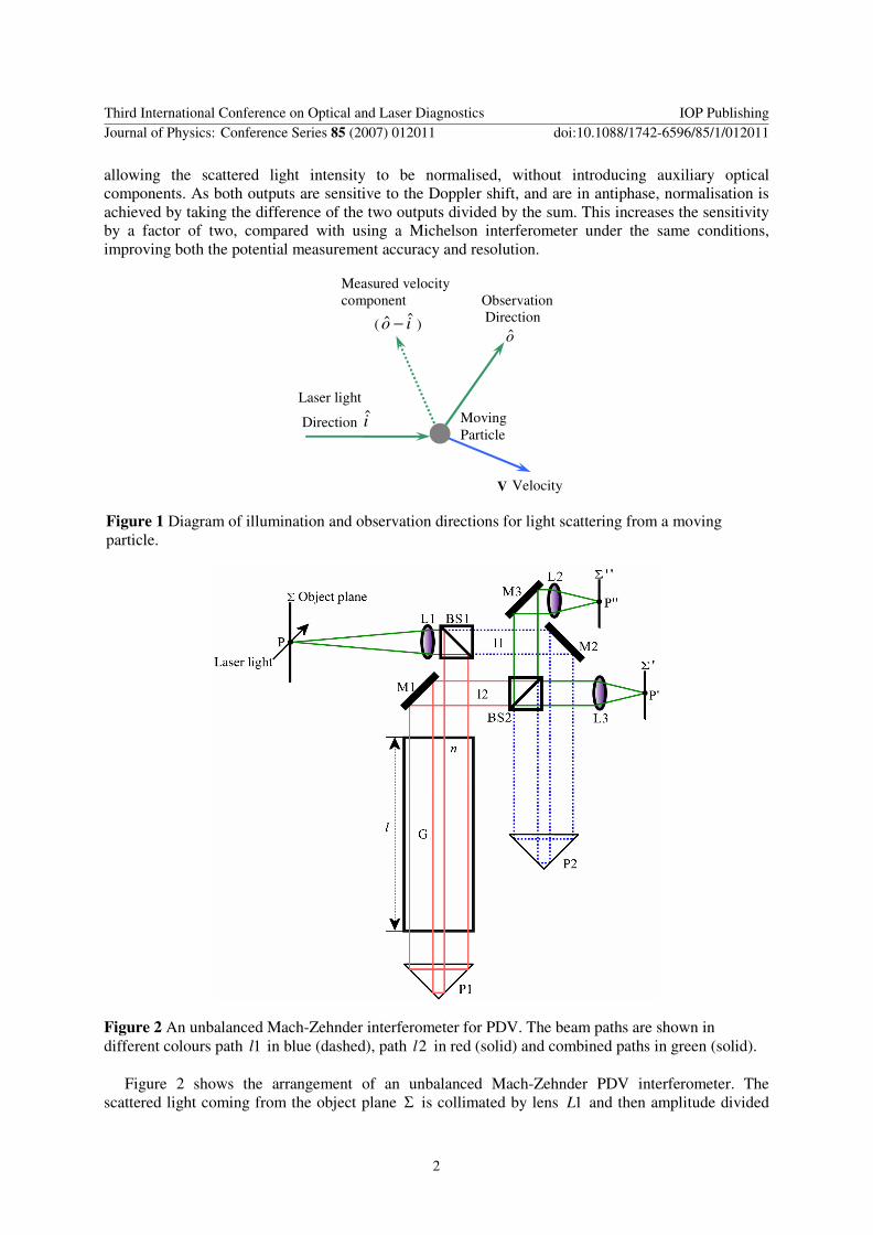
allowing the scattered light intensity to be normalised without introducing auxiliary optical components As both outputs are sensitive to the Doppler shift and are in antiphase normalisation is achieved by taking the difference of the two outputs divided by the sum This increases the sensitivity by a factor of two compared with using a Michelson interferometer under the same conditions improving both the potential measurement accuracy and resolution
Figure 1 Diagram of illumination and observation directions for light scattering from a moving particle
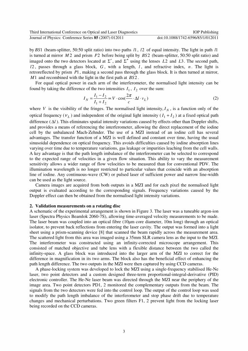
Figure 2 An unbalanced Mach-Zehnder interferometer for PDV The beam paths are shown in different colours path 1l in blue (dashed) path 2l in red (solid) and combined paths in green (solid)
Figure 2 shows the arrangement of an unbalanced Mach-Zehnder PDV interferometer The
scattered light coming from the object plane Σ is collimated by lens 1L and then amplitude divided
Measured velocity component
( io ˆˆ minus )
Observation Direction o
Laser light
Direction i
V Velocity
Moving Particle
Third International Conference on Optical and Laser Diagnostics IOP PublishingJournal of Physics Conference Series 85 (2007) 012011 doi1010881742-6596851012011
2
by 1BS (beam-splitter 5050 split ratio) into two paths 1l 2l of equal intensity The light in path 1l is turned at mirror 2M and prism 2P before being split by 2BS (beam-splitter 5050 split ratio) and imaged onto the two detectors located at Σprime and Σ primeprime using the lenses 2L and 3L The second path 2l passes through a glass block G with a length l and refractive index n The light is
retroreflected by prism 1P making a second pass through the glass block It is then turned at mirror 1M and recombined with the light in the first path at 2BS For equal optical power in each arm of the interferometer the normalised light intensity can be
found by taking the difference of the two intensities 1I 2I over the sum
)2
cos(21
21LN vl
cV
IIII
I sdot∆sdotsdotprop+minus
= π (2)
where V is the visibility of the fringes The normalised light intensity NI is a function only of the optical frequency ( Lν ) and independent of the original light intensity ( 21 II + ) at a fixed optical path difference ( l∆ ) This eliminates spatial intensity variations caused by effects other than Doppler shifts and provides a means of referencing the interferometer allowing the direct replacement of the iodine cell by the unbalanced Mach-Zehnder The use of a MZI instead of an iodine cell has several advantages The transfer function of a MZI is well defined and constant over time having the usual sinusoidal dependence on optical frequency This avoids difficulties caused by iodine absorption lines varying over time due to temperature variations gas leakage or impurities leaching from the cell walls A key advantage is that the path length imbalance of the interferometer can be selected to correspond to the expected range of velocities in a given flow situation This ability to vary the measurement sensitivity allows a wider range of flow velocities to be measured than for conventional PDV The illumination wavelength is no longer restricted to particular values that coincide with an absorption line of iodine Any continuous-wave (CW) or pulsed laser of sufficient power and narrow line-width can be used as the light source
Camera images are acquired from both outputs in a MZI and for each pixel the normalised light output is evaluated according to the corresponding signals Frequency variations caused by the Doppler effect can then be obtained from the normalised light intensity variations
2 Validation measurements on a rotating disc A schematic of the experimental arrangement is shown in Figure 3 The laser was a tuneable argon-ion laser (Spectra Physics Beamlok 2060-7S) allowing time-averaged velocity measurements to be made The laser beam was coupled into an optical fibre (10m core diameter 10m long) through an optical isolator to prevent back reflections from entering the laser cavity The output was formed into a light sheet using a prism-scanning device [8] that scanned the beam rapidly across the measurement area The scattered light from this area was imaged using a 35mm SLR camera lens as the input to the MZI The interferometer was constructed using an infinity-corrected microscope arrangement This consisted of matched objective and tube lens with a flexible distance between the two called the infinity-space A glass block was introduced into the larger arm of the MZI to correct for the difference in magnification in its two arms The block also has the beneficial effect of enhancing the path length difference The two outputs in the MZI were then captured by using CCD cameras
A phase-locking system was developed to lock the MZI using a single-frequency stabilised He-Ne laser two point detectors and a custom designed three-term proportional-integral-derivative (PID) electronic controller The He-Ne laser beam was directed through the MZI near the periphery of the image area Two point detectors PD1 2 monitored the complementary outputs from the beam The signals from the two detectors were fed into the control loop The output of the control loop was used to modify the path length imbalance of the interferometer and stop phase drift due to temperature changes and mechanical perturbations Two green filters F1 2 prevent light from the locking laser being recorded on the CCD cameras
Third International Conference on Optical and Laser Diagnostics IOP PublishingJournal of Physics Conference Series 85 (2007) 012011 doi1010881742-6596851012011
3
Figure 3 Single velocity component measurement Mach-Zehnder interferometric filter based PDV system HWP half-wave plate BS1 BS2 non-polarization beam splitters L1 standard camera lens L2 3 tube lenses L4 lens M1 2 3 4 5 mirrors F1 2 green filters P1 2 right-angle prisms
A rotating disc was used to generate a well-defined velocity field with which to characterise the
performance of the system The disk was 200mm in diameter and coated with white paint in order to enhance the light scattering The maximum velocity was ~plusmn70ms which was measured independently using an optical tachometer The observation direction was at an angle of ~18ordm to the surface of the disc measured from the centre of the disc to the centre of the imaging lens The illumination direction was at an angle of ~14ordm to the observation direction The geometry was selected to have a high sensitivity to the horizontal velocity component Figure 4 shows one pair of fringe images recorded by two cameras for the rotating disc
Two methods of calculating the velocity have been investigated the first uses the shift of the fringe pattern to determine the Doppler shift similar to the method reported by Seiler et al [9] The second provides a measurement of the Doppler shift at each pixel in the images by normalising the received light intensity using the two outputs of the MZI
Third International Conference on Optical and Laser Diagnostics IOP PublishingJournal of Physics Conference Series 85 (2007) 012011 doi1010881742-6596851012011
4
-80
-40
0
40
80
-100 -50 0 50 100Position (mm)
Vel
ocit
y (m
s)
CCD1
CCD2
Opticaltachometer
Figure 4 One pair of fringe images recorded by CCD1 (top) and CCD2 (bottom) for the rotating disc
Figure 5 Vertical velocity profile taken through the centre of the disc using the dark fringe shift method
Using the fringe shift method the velocity at each point along the fringe was calculated Figure 5
shows the computed velocity at points through the centre of the disc The solid line represents the velocity calculated from the optical tachometer measurements The velocity error for this technique is about plusmn5ms As previously mentioned the use of a MZI allows twice the number of measurement profiles compared to a Michelson interferometer using a single output the measurement profiles would be spaced at ~40pixels (22mm) apart but using the two outputs available with the MZI arrangement allows the number of profiles to be doubled giving a spacing of ~20pixels (11mm) This can be seen in Figure 5 where values from the two outputs are plotted with different symbols
X[mm]
Y[m
m]
-100 -50 0 50 100
-100
-50
0
50
100
-60
-40
-20
0
20
40
60
-80
-40
0
40
80
-100 -50 0 50 100Position (mm)
Vel
ocit
y (m
s)
PDV
Opticaltachometer
Figure 6 Computed velocity component of the rotating disc using the normalised light intensity method
Figure 7 Velocity profile taken through the centre of the disc using the normalised light intensity method
Figure 6 shows the computed horizontal velocity component made by calculating the normalised
light intensity at each pixel in the interference images Figure 7 shows a velocity profile taken through the centre of the disc The measured velocities correspond very well with the values calculated from the optical tachometer measurement The measurements towards the edge of the disc vary more from
ms
Third International Conference on Optical and Laser Diagnostics IOP PublishingJournal of Physics Conference Series 85 (2007) 012011 doi1010881742-6596851012011
5
the expected values possibly due to worse interference fringe quality in these regions and lower signal levels resulting from the lsquovignetting effectrsquo in the infinity-corrected optical system
3 Measurements on a seeded jet flow The system was used to make measurements on a seeded air jet with a 20mm diameter smooth contraction nozzle [5] The exit velocity of the jet is ~85ms The air intake to the jet and the surrounding co-flow were seeded using a Concept Engineering ViCount compact smoke generator which produces particles in the 02-03m-diameter range The main flow direction was opposite to the laser illumination direction and the observation direction perpendicular to this This provides a measured velocity component that is at an angle of ~45ordm from the main flow direction The measured area was approximately 50x50mm and a camera exposure time of 10 seconds was used
X[mm]
Y[m
m]
50 40 30 20 10 0
-10
0
10 20
40
60
80
100
Figure 8 One pair of fringe images recorded by CCD1 (top) and CCD2 (bottom) for the jet flow
Figure 9 The computed velocity component of the air jet flow made using the MZI-PDV system (the area in the rectangle in Figure 8)
One pair of images recorded by the two cameras for the jet flow is shown in Figure 8 The data was
first processed using the fringe shifting method and the results are shown Figure 10 This shows the computed velocity profiles vertically across the main flow direction along with the theoretical velocity distribution derived from knowledge of the jet dimensions and the exit velocity [10] The profiles are located at 05 1 15 2 and 25 diameters downstream from the nozzle (xd) There is good agreement between the two sets of profiles The steps in the measured velocities are due to the processing method whereby only whole pixel shifts can be measured
Figure 9 shows the computed velocity component based on calculating the normalised light intensity at each pixel Figure 11 shows the computed velocity component profiles vertically across the main flow direction along with the theoretical velocity distribution The profiles are located at 05 1 15 2 and 25 diameters downstream from the nozzle There is generally good agreement between the two sets of profiles
Because of optical distortions the fringe amplitude in some regions is less than unity To correct for this the nearest maximum and minimum are located for each pixel allowing the local fringe amplitude to be measured This is used to remove amplitude variations in the fringe pattern
The lsquostripingrsquo effect in the image in Figure 9 results from the processing method Close to maxima and minima the velocity sensitivity is lower than at the quadrature positions Also small deviations from a sinusoidal form resulting from smoothing are largest close to maximaminima and can result in slight velocity errors
ms
Third International Conference on Optical and Laser Diagnostics IOP PublishingJournal of Physics Conference Series 85 (2007) 012011 doi1010881742-6596851012011
6
The measurements towards the outside edge of the jet flow vary more from the calculated values than those at the centre This is attributed to worse interference fringe quality in these regions lower signal levels resulting from the lsquovignetting effectrsquo in the infinity-corrected optical system and lower seeding levels in these regions as well The uneven power distribution in the illumination light sheet results in reduced fringe quality away from the image centre as seen in Figure 8 The magnitudes differ between the two sets of values This can be explained by the simplified empirical equations used to calculate the theoretical profiles and possible differences between the theoretical jet flow and that generated by the real jet
0
50
100
-20 -10 0 10 20Position (mm)
Vel
ocit
y (m
s)
xd = 25
0
50
100
-20 -10 0 10 20Position (mm)
Vel
ocit
y (m
s)
xd = 25
0
50
100
-20 -10 0 10 20Position (mm)
Vel
ocit
y (m
s)
xd = 2
0
50
100
-20 -10 0 10 20Position (mm)
Vel
ocit
y (m
s)
xd = 2
0
50
100
-20 -10 0 10 20Position (mm)
Vel
ocit
y (m
s)
xd = 15
0
50
100
-20 -10 0 10 20Position (mm)
Vel
ocit
y (m
s)
xd = 15
0
50
100
-20 -10 0 10 20Position (mm)
Vel
ocit
y (m
s)
xd = 1
0
50
100
-20 -10 0 10 20Position (mm)
Vel
ocit
y (m
s)
xd = 1
0
50
100
-20 -10 0 10 20Position (mm)
Vel
ocit
y (m
s)
xd = 05
0
50
100
-20 -10 0 10 20Position (mm)
Vel
ocit
y (m
s)
xd = 05
Figure 10 A comparison between computed velocity profiles taken thorough the centre of the jet at xd = 05 1 15 2 and 25 diameters downstream from the nozzle using the fringe shift method and the theoretical jet profile mdash Theoretical values times MZI-PDV
Figure 11 A comparison between computed velocity profiles taken thorough the centre of the air jet at xd = 05 1 15 2 and 25 diameters downstream from the nozzle using the normalised light intensity method and the theoretical jet profile mdash Theoretical values times MZI-PDV
Third International Conference on Optical and Laser Diagnostics IOP PublishingJournal of Physics Conference Series 85 (2007) 012011 doi1010881742-6596851012011
7
4 Conclusions A Mach-Zehnder interferometric filter based planar Doppler velocimeter has been demonstrated The results of measurements from a rotating disc have been used to validate this system It has several advantages over an iodine cell based system The path length imbalance can be selected to correspond to the expected range of velocities in a given flow situation The illumination wavelength is no longer restricted to particular values Any cw or pulsed laser of sufficient power can be used as the light source The MZI provides normalised light intensity automatically based on its complementary outputs while a Michelson interferometer cannot do this without additional optical components
Measurements on a seeded air jet were made demonstrating good agreement with the expected velocities calculated using empirical equations for the jet velocity profile
Acknowledgements Zenghai Lu acknowledges an Overseas Research Scholarship (ORS) award from the Committee of Vice Chancellors and Principals UK This work was supported by a Paul Instrument Fund grant from the Royal Society UK
References [1] Elliott Gregory S and Beutner Thomas J 1999 Molecular filter based planar Doppler velocimetry Progress
in Aerospace Sciences 35 799-845
[2] Elliott G S Crafton J Baust H D Beutner T J Carter C D and Tyler C 2005 Evaluation and optimization of a multi-component planar Doppler velocimetry system 43rd AIAA Aerospace Sciences Meeting and Exhibit Reno NV United States 6695-6717
[3] Ford H D and Tatam R P 1997 Development of extended field Doppler velocimetry for turbomachinery applications Optics and Lasers in Engineering 27 675-96
[4] Nobes D S Ford H D and Tatam R P 2004 Instantaneous three-component planar Doppler velocimetry using imaging fibre bundles Experiments in Fluids 36 3-10
[5] Charrett T O H and Tatam R P 2006 Single camera three component planar velocity measurements using two-frequency planar Doppler velocimetry (2v-PDV) Measurement Science and Technology 17 1194-1206
[6] Komine H Brosnan S Litton A and Stappaers E 1991 Real-Time Doppler Global Velocimetry AIAA 29th Aerospace Sciences Meeting Reno NV Paper 91-0337
[7] Ainsworth R W Thorpe S J and Manners R J 1997 New approach to flow-field measurement - a view of Doppler global velocimetry techniques International Journal of Heat and Fluid Flow 18 116-130
[8] Roehle I Schodl R Voigt P and Willert C 2000 Recent developments and applications of quantitative laser light sheet measuring techniques in turbomachinery components Measurement Science and Technology 11 1023-35
[9] Seiler F Havermann M George A Leopold F and Srulijes J 2003 Planar velocity visualization in high-speed wedge flow using Doppler picture velocimetry (DPV) compared with particle image velocimetry (PIV) Journal of Visualization 6 253-62
[10] Rajaratnam N 1976 Turbulent jets Elsevier Amsterdam Netherlands
Third International Conference on Optical and Laser Diagnostics IOP PublishingJournal of Physics Conference Series 85 (2007) 012011 doi1010881742-6596851012011
8
Planar Doppler velocimetry using a Mach-Zehnder interferometric filter
Z-H Lu T O H Charrett H D Ford and R P Tatam
Engineering Photonics Group School of Engineering Cranfield University Cranfield Bedford MK43 OAL UK
Email rptatamcranfieldacuk
Abstract A planar Doppler velocimetry system to measure flow velocity fields is described The technique uses a Mach-Zehnder interferometric filter to convert Doppler frequency shifts into intensity variations The free spectral range of the filter can be selected by adjusting the optical path difference of the interferometer This allows the velocity measurement range sensitivity and resolution to be varied An experimental arrangement is described that incorporates a phase-locking system designed to stabilise the interferometric filter Two methods to process the interference fringe images are presented the first uses the shift of the fringe pattern to determine the Doppler shift along profiles The second provides a full-field measurement of the Doppler shift by determining the phase at each pixel in the images Results are presented here for measurements of velocity fields on a rotating disc with maximum velocities at the edge of plusmn70ms Measurements on a seeded air jet with a nozzle diameter of 20mm and an exit velocity of ~85ms are also presented
1 Introduction Planar Doppler Velocimetry (PDV) [1-5] also called Doppler Global Velocimetry (DGV) [67] measures the Doppler shift in the laser light scattered by particles embedded in a flow and thus determines the flow velocity using the Doppler equation (1)
c
)io(vv L Vsdotminus
=∆ˆˆ
(1)
where Lννν minus=∆ is the difference between the scattered light frequency ν and the original laser light frequency Lν V is the velocity vector associated with the scattering particles and c the free
space speed of light o and i are unit vectors in the observation and illumination directions respectively (Figure 1) In PDV the Doppler shift is measured at each pixel in a CCD camera image of the flow which is illuminated using a laser light sheet Measurement of the frequency shift is achieved using a frequency-to-intensity converter to date the most common method has been to use a molecular filter typically iodine vapour By selecting the illumination frequency to coincide with an absorption line the received intensity at the CCD camera is related to the Doppler shift and hence the flow velocity A reference camera viewing the flow directly is needed to normalise the signal for differences in scattered light intensity
This paper investigates a PDV system using a Mach-Zehnder interferometric filter (MZI) instead of a molecular filter The use of a Mach-Zehnder interferometer provides two complementary outputs
Third International Conference on Optical and Laser Diagnostics IOP PublishingJournal of Physics Conference Series 85 (2007) 012011 doi1010881742-6596851012011
ccopy 2007 IOP Publishing Ltd 1
allowing the scattered light intensity to be normalised without introducing auxiliary optical components As both outputs are sensitive to the Doppler shift and are in antiphase normalisation is achieved by taking the difference of the two outputs divided by the sum This increases the sensitivity by a factor of two compared with using a Michelson interferometer under the same conditions improving both the potential measurement accuracy and resolution
Figure 1 Diagram of illumination and observation directions for light scattering from a moving particle
Figure 2 An unbalanced Mach-Zehnder interferometer for PDV The beam paths are shown in different colours path 1l in blue (dashed) path 2l in red (solid) and combined paths in green (solid)
Figure 2 shows the arrangement of an unbalanced Mach-Zehnder PDV interferometer The
scattered light coming from the object plane Σ is collimated by lens 1L and then amplitude divided
Measured velocity component
( io ˆˆ minus )
Observation Direction o
Laser light
Direction i
V Velocity
Moving Particle
Third International Conference on Optical and Laser Diagnostics IOP PublishingJournal of Physics Conference Series 85 (2007) 012011 doi1010881742-6596851012011
2
by 1BS (beam-splitter 5050 split ratio) into two paths 1l 2l of equal intensity The light in path 1l is turned at mirror 2M and prism 2P before being split by 2BS (beam-splitter 5050 split ratio) and imaged onto the two detectors located at Σprime and Σ primeprime using the lenses 2L and 3L The second path 2l passes through a glass block G with a length l and refractive index n The light is
retroreflected by prism 1P making a second pass through the glass block It is then turned at mirror 1M and recombined with the light in the first path at 2BS For equal optical power in each arm of the interferometer the normalised light intensity can be
found by taking the difference of the two intensities 1I 2I over the sum
)2
cos(21
21LN vl
cV
IIII
I sdot∆sdotsdotprop+minus
= π (2)
where V is the visibility of the fringes The normalised light intensity NI is a function only of the optical frequency ( Lν ) and independent of the original light intensity ( 21 II + ) at a fixed optical path difference ( l∆ ) This eliminates spatial intensity variations caused by effects other than Doppler shifts and provides a means of referencing the interferometer allowing the direct replacement of the iodine cell by the unbalanced Mach-Zehnder The use of a MZI instead of an iodine cell has several advantages The transfer function of a MZI is well defined and constant over time having the usual sinusoidal dependence on optical frequency This avoids difficulties caused by iodine absorption lines varying over time due to temperature variations gas leakage or impurities leaching from the cell walls A key advantage is that the path length imbalance of the interferometer can be selected to correspond to the expected range of velocities in a given flow situation This ability to vary the measurement sensitivity allows a wider range of flow velocities to be measured than for conventional PDV The illumination wavelength is no longer restricted to particular values that coincide with an absorption line of iodine Any continuous-wave (CW) or pulsed laser of sufficient power and narrow line-width can be used as the light source
Camera images are acquired from both outputs in a MZI and for each pixel the normalised light output is evaluated according to the corresponding signals Frequency variations caused by the Doppler effect can then be obtained from the normalised light intensity variations
2 Validation measurements on a rotating disc A schematic of the experimental arrangement is shown in Figure 3 The laser was a tuneable argon-ion laser (Spectra Physics Beamlok 2060-7S) allowing time-averaged velocity measurements to be made The laser beam was coupled into an optical fibre (10m core diameter 10m long) through an optical isolator to prevent back reflections from entering the laser cavity The output was formed into a light sheet using a prism-scanning device [8] that scanned the beam rapidly across the measurement area The scattered light from this area was imaged using a 35mm SLR camera lens as the input to the MZI The interferometer was constructed using an infinity-corrected microscope arrangement This consisted of matched objective and tube lens with a flexible distance between the two called the infinity-space A glass block was introduced into the larger arm of the MZI to correct for the difference in magnification in its two arms The block also has the beneficial effect of enhancing the path length difference The two outputs in the MZI were then captured by using CCD cameras
A phase-locking system was developed to lock the MZI using a single-frequency stabilised He-Ne laser two point detectors and a custom designed three-term proportional-integral-derivative (PID) electronic controller The He-Ne laser beam was directed through the MZI near the periphery of the image area Two point detectors PD1 2 monitored the complementary outputs from the beam The signals from the two detectors were fed into the control loop The output of the control loop was used to modify the path length imbalance of the interferometer and stop phase drift due to temperature changes and mechanical perturbations Two green filters F1 2 prevent light from the locking laser being recorded on the CCD cameras
Third International Conference on Optical and Laser Diagnostics IOP PublishingJournal of Physics Conference Series 85 (2007) 012011 doi1010881742-6596851012011
3
Figure 3 Single velocity component measurement Mach-Zehnder interferometric filter based PDV system HWP half-wave plate BS1 BS2 non-polarization beam splitters L1 standard camera lens L2 3 tube lenses L4 lens M1 2 3 4 5 mirrors F1 2 green filters P1 2 right-angle prisms
A rotating disc was used to generate a well-defined velocity field with which to characterise the
performance of the system The disk was 200mm in diameter and coated with white paint in order to enhance the light scattering The maximum velocity was ~plusmn70ms which was measured independently using an optical tachometer The observation direction was at an angle of ~18ordm to the surface of the disc measured from the centre of the disc to the centre of the imaging lens The illumination direction was at an angle of ~14ordm to the observation direction The geometry was selected to have a high sensitivity to the horizontal velocity component Figure 4 shows one pair of fringe images recorded by two cameras for the rotating disc
Two methods of calculating the velocity have been investigated the first uses the shift of the fringe pattern to determine the Doppler shift similar to the method reported by Seiler et al [9] The second provides a measurement of the Doppler shift at each pixel in the images by normalising the received light intensity using the two outputs of the MZI
Third International Conference on Optical and Laser Diagnostics IOP PublishingJournal of Physics Conference Series 85 (2007) 012011 doi1010881742-6596851012011
4
-80
-40
0
40
80
-100 -50 0 50 100Position (mm)
Vel
ocit
y (m
s)
CCD1
CCD2
Opticaltachometer
Figure 4 One pair of fringe images recorded by CCD1 (top) and CCD2 (bottom) for the rotating disc
Figure 5 Vertical velocity profile taken through the centre of the disc using the dark fringe shift method
Using the fringe shift method the velocity at each point along the fringe was calculated Figure 5
shows the computed velocity at points through the centre of the disc The solid line represents the velocity calculated from the optical tachometer measurements The velocity error for this technique is about plusmn5ms As previously mentioned the use of a MZI allows twice the number of measurement profiles compared to a Michelson interferometer using a single output the measurement profiles would be spaced at ~40pixels (22mm) apart but using the two outputs available with the MZI arrangement allows the number of profiles to be doubled giving a spacing of ~20pixels (11mm) This can be seen in Figure 5 where values from the two outputs are plotted with different symbols
X[mm]
Y[m
m]
-100 -50 0 50 100
-100
-50
0
50
100
-60
-40
-20
0
20
40
60
-80
-40
0
40
80
-100 -50 0 50 100Position (mm)
Vel
ocit
y (m
s)
PDV
Opticaltachometer
Figure 6 Computed velocity component of the rotating disc using the normalised light intensity method
Figure 7 Velocity profile taken through the centre of the disc using the normalised light intensity method
Figure 6 shows the computed horizontal velocity component made by calculating the normalised
light intensity at each pixel in the interference images Figure 7 shows a velocity profile taken through the centre of the disc The measured velocities correspond very well with the values calculated from the optical tachometer measurement The measurements towards the edge of the disc vary more from
ms
Third International Conference on Optical and Laser Diagnostics IOP PublishingJournal of Physics Conference Series 85 (2007) 012011 doi1010881742-6596851012011
5
the expected values possibly due to worse interference fringe quality in these regions and lower signal levels resulting from the lsquovignetting effectrsquo in the infinity-corrected optical system
3 Measurements on a seeded jet flow The system was used to make measurements on a seeded air jet with a 20mm diameter smooth contraction nozzle [5] The exit velocity of the jet is ~85ms The air intake to the jet and the surrounding co-flow were seeded using a Concept Engineering ViCount compact smoke generator which produces particles in the 02-03m-diameter range The main flow direction was opposite to the laser illumination direction and the observation direction perpendicular to this This provides a measured velocity component that is at an angle of ~45ordm from the main flow direction The measured area was approximately 50x50mm and a camera exposure time of 10 seconds was used
X[mm]
Y[m
m]
50 40 30 20 10 0
-10
0
10 20
40
60
80
100
Figure 8 One pair of fringe images recorded by CCD1 (top) and CCD2 (bottom) for the jet flow
Figure 9 The computed velocity component of the air jet flow made using the MZI-PDV system (the area in the rectangle in Figure 8)
One pair of images recorded by the two cameras for the jet flow is shown in Figure 8 The data was
first processed using the fringe shifting method and the results are shown Figure 10 This shows the computed velocity profiles vertically across the main flow direction along with the theoretical velocity distribution derived from knowledge of the jet dimensions and the exit velocity [10] The profiles are located at 05 1 15 2 and 25 diameters downstream from the nozzle (xd) There is good agreement between the two sets of profiles The steps in the measured velocities are due to the processing method whereby only whole pixel shifts can be measured
Figure 9 shows the computed velocity component based on calculating the normalised light intensity at each pixel Figure 11 shows the computed velocity component profiles vertically across the main flow direction along with the theoretical velocity distribution The profiles are located at 05 1 15 2 and 25 diameters downstream from the nozzle There is generally good agreement between the two sets of profiles
Because of optical distortions the fringe amplitude in some regions is less than unity To correct for this the nearest maximum and minimum are located for each pixel allowing the local fringe amplitude to be measured This is used to remove amplitude variations in the fringe pattern
The lsquostripingrsquo effect in the image in Figure 9 results from the processing method Close to maxima and minima the velocity sensitivity is lower than at the quadrature positions Also small deviations from a sinusoidal form resulting from smoothing are largest close to maximaminima and can result in slight velocity errors
ms
Third International Conference on Optical and Laser Diagnostics IOP PublishingJournal of Physics Conference Series 85 (2007) 012011 doi1010881742-6596851012011
6
The measurements towards the outside edge of the jet flow vary more from the calculated values than those at the centre This is attributed to worse interference fringe quality in these regions lower signal levels resulting from the lsquovignetting effectrsquo in the infinity-corrected optical system and lower seeding levels in these regions as well The uneven power distribution in the illumination light sheet results in reduced fringe quality away from the image centre as seen in Figure 8 The magnitudes differ between the two sets of values This can be explained by the simplified empirical equations used to calculate the theoretical profiles and possible differences between the theoretical jet flow and that generated by the real jet
0
50
100
-20 -10 0 10 20Position (mm)
Vel
ocit
y (m
s)
xd = 25
0
50
100
-20 -10 0 10 20Position (mm)
Vel
ocit
y (m
s)
xd = 25
0
50
100
-20 -10 0 10 20Position (mm)
Vel
ocit
y (m
s)
xd = 2
0
50
100
-20 -10 0 10 20Position (mm)
Vel
ocit
y (m
s)
xd = 2
0
50
100
-20 -10 0 10 20Position (mm)
Vel
ocit
y (m
s)
xd = 15
0
50
100
-20 -10 0 10 20Position (mm)
Vel
ocit
y (m
s)
xd = 15
0
50
100
-20 -10 0 10 20Position (mm)
Vel
ocit
y (m
s)
xd = 1
0
50
100
-20 -10 0 10 20Position (mm)
Vel
ocit
y (m
s)
xd = 1
0
50
100
-20 -10 0 10 20Position (mm)
Vel
ocit
y (m
s)
xd = 05
0
50
100
-20 -10 0 10 20Position (mm)
Vel
ocit
y (m
s)
xd = 05
Figure 10 A comparison between computed velocity profiles taken thorough the centre of the jet at xd = 05 1 15 2 and 25 diameters downstream from the nozzle using the fringe shift method and the theoretical jet profile mdash Theoretical values times MZI-PDV
Figure 11 A comparison between computed velocity profiles taken thorough the centre of the air jet at xd = 05 1 15 2 and 25 diameters downstream from the nozzle using the normalised light intensity method and the theoretical jet profile mdash Theoretical values times MZI-PDV
Third International Conference on Optical and Laser Diagnostics IOP PublishingJournal of Physics Conference Series 85 (2007) 012011 doi1010881742-6596851012011
7
4 Conclusions A Mach-Zehnder interferometric filter based planar Doppler velocimeter has been demonstrated The results of measurements from a rotating disc have been used to validate this system It has several advantages over an iodine cell based system The path length imbalance can be selected to correspond to the expected range of velocities in a given flow situation The illumination wavelength is no longer restricted to particular values Any cw or pulsed laser of sufficient power can be used as the light source The MZI provides normalised light intensity automatically based on its complementary outputs while a Michelson interferometer cannot do this without additional optical components
Measurements on a seeded air jet were made demonstrating good agreement with the expected velocities calculated using empirical equations for the jet velocity profile
Acknowledgements Zenghai Lu acknowledges an Overseas Research Scholarship (ORS) award from the Committee of Vice Chancellors and Principals UK This work was supported by a Paul Instrument Fund grant from the Royal Society UK
References [1] Elliott Gregory S and Beutner Thomas J 1999 Molecular filter based planar Doppler velocimetry Progress
in Aerospace Sciences 35 799-845
[2] Elliott G S Crafton J Baust H D Beutner T J Carter C D and Tyler C 2005 Evaluation and optimization of a multi-component planar Doppler velocimetry system 43rd AIAA Aerospace Sciences Meeting and Exhibit Reno NV United States 6695-6717
[3] Ford H D and Tatam R P 1997 Development of extended field Doppler velocimetry for turbomachinery applications Optics and Lasers in Engineering 27 675-96
[4] Nobes D S Ford H D and Tatam R P 2004 Instantaneous three-component planar Doppler velocimetry using imaging fibre bundles Experiments in Fluids 36 3-10
[5] Charrett T O H and Tatam R P 2006 Single camera three component planar velocity measurements using two-frequency planar Doppler velocimetry (2v-PDV) Measurement Science and Technology 17 1194-1206
[6] Komine H Brosnan S Litton A and Stappaers E 1991 Real-Time Doppler Global Velocimetry AIAA 29th Aerospace Sciences Meeting Reno NV Paper 91-0337
[7] Ainsworth R W Thorpe S J and Manners R J 1997 New approach to flow-field measurement - a view of Doppler global velocimetry techniques International Journal of Heat and Fluid Flow 18 116-130
[8] Roehle I Schodl R Voigt P and Willert C 2000 Recent developments and applications of quantitative laser light sheet measuring techniques in turbomachinery components Measurement Science and Technology 11 1023-35
[9] Seiler F Havermann M George A Leopold F and Srulijes J 2003 Planar velocity visualization in high-speed wedge flow using Doppler picture velocimetry (DPV) compared with particle image velocimetry (PIV) Journal of Visualization 6 253-62
[10] Rajaratnam N 1976 Turbulent jets Elsevier Amsterdam Netherlands
Third International Conference on Optical and Laser Diagnostics IOP PublishingJournal of Physics Conference Series 85 (2007) 012011 doi1010881742-6596851012011
8
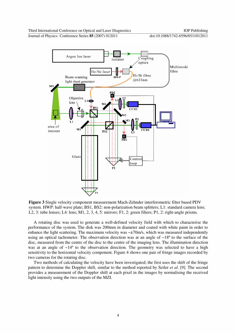
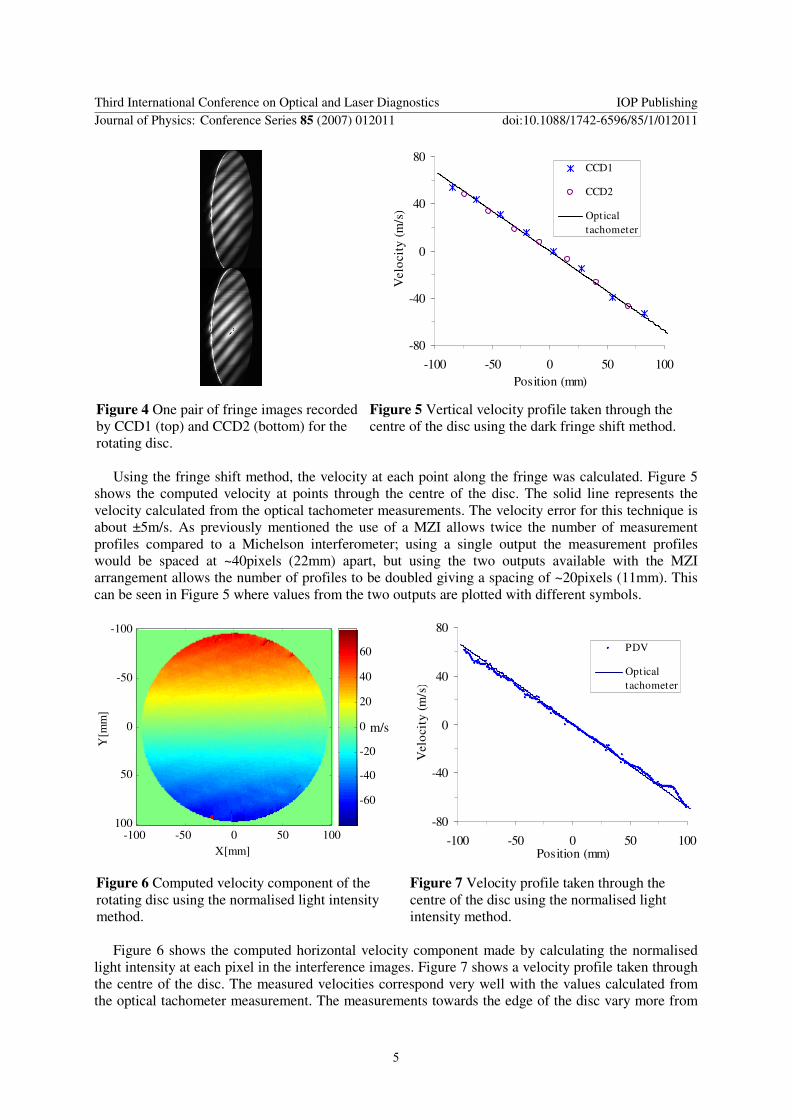
-80
-40
0
40
80
-100 -50 0 50 100Position (mm)
Vel
ocit
y (m
s)
CCD1
CCD2
Opticaltachometer
Figure 4 One pair of fringe images recorded by CCD1 (top) and CCD2 (bottom) for the rotating disc
Figure 5 Vertical velocity profile taken through the centre of the disc using the dark fringe shift method
Using the fringe shift method the velocity at each point along the fringe was calculated Figure 5
shows the computed velocity at points through the centre of the disc The solid line represents the velocity calculated from the optical tachometer measurements The velocity error for this technique is about plusmn5ms As previously mentioned the use of a MZI allows twice the number of measurement profiles compared to a Michelson interferometer using a single output the measurement profiles would be spaced at ~40pixels (22mm) apart but using the two outputs available with the MZI arrangement allows the number of profiles to be doubled giving a spacing of ~20pixels (11mm) This can be seen in Figure 5 where values from the two outputs are plotted with different symbols
X[mm]
Y[m
m]
-100 -50 0 50 100
-100
-50
0
50
100
-60
-40
-20
0
20
40
60
-80
-40
0
40
80
-100 -50 0 50 100Position (mm)
Vel
ocit
y (m
s)
PDV
Opticaltachometer
Figure 6 Computed velocity component of the rotating disc using the normalised light intensity method
Figure 7 Velocity profile taken through the centre of the disc using the normalised light intensity method
Figure 6 shows the computed horizontal velocity component made by calculating the normalised
light intensity at each pixel in the interference images Figure 7 shows a velocity profile taken through the centre of the disc The measured velocities correspond very well with the values calculated from the optical tachometer measurement The measurements towards the edge of the disc vary more from
ms
Third International Conference on Optical and Laser Diagnostics IOP PublishingJournal of Physics Conference Series 85 (2007) 012011 doi1010881742-6596851012011
5
the expected values possibly due to worse interference fringe quality in these regions and lower signal levels resulting from the lsquovignetting effectrsquo in the infinity-corrected optical system
3 Measurements on a seeded jet flow The system was used to make measurements on a seeded air jet with a 20mm diameter smooth contraction nozzle [5] The exit velocity of the jet is ~85ms The air intake to the jet and the surrounding co-flow were seeded using a Concept Engineering ViCount compact smoke generator which produces particles in the 02-03m-diameter range The main flow direction was opposite to the laser illumination direction and the observation direction perpendicular to this This provides a measured velocity component that is at an angle of ~45ordm from the main flow direction The measured area was approximately 50x50mm and a camera exposure time of 10 seconds was used
X[mm]
Y[m
m]
50 40 30 20 10 0
-10
0
10 20
40
60
80
100
Figure 8 One pair of fringe images recorded by CCD1 (top) and CCD2 (bottom) for the jet flow
Figure 9 The computed velocity component of the air jet flow made using the MZI-PDV system (the area in the rectangle in Figure 8)
One pair of images recorded by the two cameras for the jet flow is shown in Figure 8 The data was
first processed using the fringe shifting method and the results are shown Figure 10 This shows the computed velocity profiles vertically across the main flow direction along with the theoretical velocity distribution derived from knowledge of the jet dimensions and the exit velocity [10] The profiles are located at 05 1 15 2 and 25 diameters downstream from the nozzle (xd) There is good agreement between the two sets of profiles The steps in the measured velocities are due to the processing method whereby only whole pixel shifts can be measured
Figure 9 shows the computed velocity component based on calculating the normalised light intensity at each pixel Figure 11 shows the computed velocity component profiles vertically across the main flow direction along with the theoretical velocity distribution The profiles are located at 05 1 15 2 and 25 diameters downstream from the nozzle There is generally good agreement between the two sets of profiles
Because of optical distortions the fringe amplitude in some regions is less than unity To correct for this the nearest maximum and minimum are located for each pixel allowing the local fringe amplitude to be measured This is used to remove amplitude variations in the fringe pattern
The lsquostripingrsquo effect in the image in Figure 9 results from the processing method Close to maxima and minima the velocity sensitivity is lower than at the quadrature positions Also small deviations from a sinusoidal form resulting from smoothing are largest close to maximaminima and can result in slight velocity errors
ms
Third International Conference on Optical and Laser Diagnostics IOP PublishingJournal of Physics Conference Series 85 (2007) 012011 doi1010881742-6596851012011
6
The measurements towards the outside edge of the jet flow vary more from the calculated values than those at the centre This is attributed to worse interference fringe quality in these regions lower signal levels resulting from the lsquovignetting effectrsquo in the infinity-corrected optical system and lower seeding levels in these regions as well The uneven power distribution in the illumination light sheet results in reduced fringe quality away from the image centre as seen in Figure 8 The magnitudes differ between the two sets of values This can be explained by the simplified empirical equations used to calculate the theoretical profiles and possible differences between the theoretical jet flow and that generated by the real jet
0
50
100
-20 -10 0 10 20Position (mm)
Vel
ocit
y (m
s)
xd = 25
0
50
100
-20 -10 0 10 20Position (mm)
Vel
ocit
y (m
s)
xd = 25
0
50
100
-20 -10 0 10 20Position (mm)
Vel
ocit
y (m
s)
xd = 2
0
50
100
-20 -10 0 10 20Position (mm)
Vel
ocit
y (m
s)
xd = 2
0
50
100
-20 -10 0 10 20Position (mm)
Vel
ocit
y (m
s)
xd = 15
0
50
100
-20 -10 0 10 20Position (mm)
Vel
ocit
y (m
s)
xd = 15
0
50
100
-20 -10 0 10 20Position (mm)
Vel
ocit
y (m
s)
xd = 1
0
50
100
-20 -10 0 10 20Position (mm)
Vel
ocit
y (m
s)
xd = 1
0
50
100
-20 -10 0 10 20Position (mm)
Vel
ocit
y (m
s)
xd = 05
0
50
100
-20 -10 0 10 20Position (mm)
Vel
ocit
y (m
s)
xd = 05
Figure 10 A comparison between computed velocity profiles taken thorough the centre of the jet at xd = 05 1 15 2 and 25 diameters downstream from the nozzle using the fringe shift method and the theoretical jet profile mdash Theoretical values times MZI-PDV
Figure 11 A comparison between computed velocity profiles taken thorough the centre of the air jet at xd = 05 1 15 2 and 25 diameters downstream from the nozzle using the normalised light intensity method and the theoretical jet profile mdash Theoretical values times MZI-PDV
Third International Conference on Optical and Laser Diagnostics IOP PublishingJournal of Physics Conference Series 85 (2007) 012011 doi1010881742-6596851012011
7
4 Conclusions A Mach-Zehnder interferometric filter based planar Doppler velocimeter has been demonstrated The results of measurements from a rotating disc have been used to validate this system It has several advantages over an iodine cell based system The path length imbalance can be selected to correspond to the expected range of velocities in a given flow situation The illumination wavelength is no longer restricted to particular values Any cw or pulsed laser of sufficient power can be used as the light source The MZI provides normalised light intensity automatically based on its complementary outputs while a Michelson interferometer cannot do this without additional optical components
Measurements on a seeded air jet were made demonstrating good agreement with the expected velocities calculated using empirical equations for the jet velocity profile
Acknowledgements Zenghai Lu acknowledges an Overseas Research Scholarship (ORS) award from the Committee of Vice Chancellors and Principals UK This work was supported by a Paul Instrument Fund grant from the Royal Society UK
References [1] Elliott Gregory S and Beutner Thomas J 1999 Molecular filter based planar Doppler velocimetry Progress
in Aerospace Sciences 35 799-845
[2] Elliott G S Crafton J Baust H D Beutner T J Carter C D and Tyler C 2005 Evaluation and optimization of a multi-component planar Doppler velocimetry system 43rd AIAA Aerospace Sciences Meeting and Exhibit Reno NV United States 6695-6717
[3] Ford H D and Tatam R P 1997 Development of extended field Doppler velocimetry for turbomachinery applications Optics and Lasers in Engineering 27 675-96
[4] Nobes D S Ford H D and Tatam R P 2004 Instantaneous three-component planar Doppler velocimetry using imaging fibre bundles Experiments in Fluids 36 3-10
[5] Charrett T O H and Tatam R P 2006 Single camera three component planar velocity measurements using two-frequency planar Doppler velocimetry (2v-PDV) Measurement Science and Technology 17 1194-1206
[6] Komine H Brosnan S Litton A and Stappaers E 1991 Real-Time Doppler Global Velocimetry AIAA 29th Aerospace Sciences Meeting Reno NV Paper 91-0337
[7] Ainsworth R W Thorpe S J and Manners R J 1997 New approach to flow-field measurement - a view of Doppler global velocimetry techniques International Journal of Heat and Fluid Flow 18 116-130
[8] Roehle I Schodl R Voigt P and Willert C 2000 Recent developments and applications of quantitative laser light sheet measuring techniques in turbomachinery components Measurement Science and Technology 11 1023-35
[9] Seiler F Havermann M George A Leopold F and Srulijes J 2003 Planar velocity visualization in high-speed wedge flow using Doppler picture velocimetry (DPV) compared with particle image velocimetry (PIV) Journal of Visualization 6 253-62
[10] Rajaratnam N 1976 Turbulent jets Elsevier Amsterdam Netherlands
Third International Conference on Optical and Laser Diagnostics IOP PublishingJournal of Physics Conference Series 85 (2007) 012011 doi1010881742-6596851012011
8
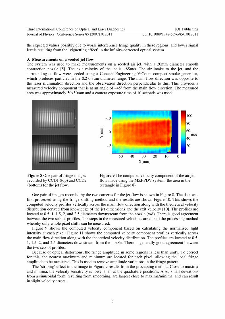
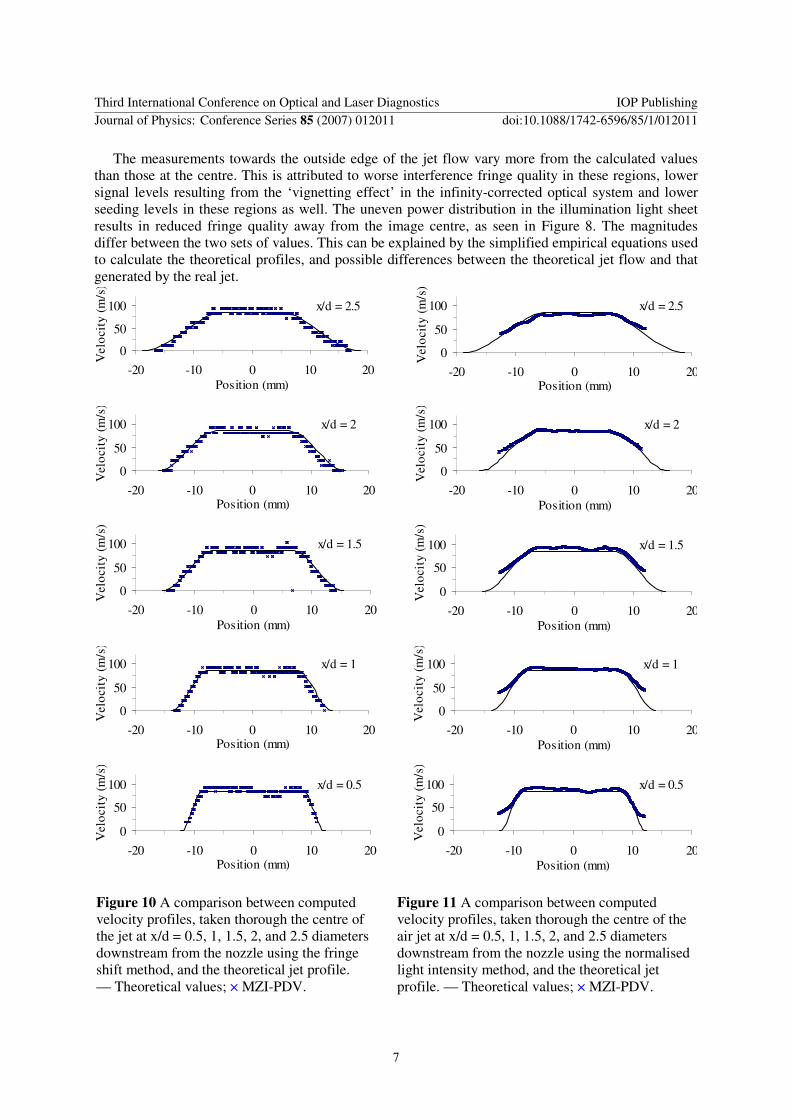