PivotTables: Easily Organize, Summarize, and Analyze Data

PivotTables: Easily Organize, Summarize, and Analyze Data

Patricia McCarthy

Course # 2164542, Version 2007, 5 CPE Credits

Course CPE Information

i

Course CPE Information Course Expiration Date Per AICPA and NASBA Standards (S9-06), QAS Self-Study courses must include an expiration date that is no longer than one year from the date of purchase or enrollment. Field of Study Computer Software & Applications. Some state boards may count credits under different categories—check with your state board for more information. Course Level Intermediate. Prerequisites Familiarity with Excel. Advance Preparation Designed for Excel 2019 and Microsoft 365 users, however excel 2010 and 2013 users should experience little difficulty. This course is NOT intended for 2007 or earlier versions of Excel. Course Description PivotTables are one of Excel’s best features. They allow you to slice and dice complex data so you can analyze it in a variety of ways. If you have ever had a large list of data and tried to analyze it or predict a trend from just looking at the numbers, then you know how difficult that can be. This course will help you maximize the flexibility of PivotTables by showing you how to easily move, summarize, analyze, and interact with data in a variety of ways. Helpful tips and exercises presented in the course make this a valuable and hands-on resource. © Copyright Mill Creek Publishing LLC 2020 Publication/Revision Date July 2020

Instructional Design

ii

Instructional Design This Self-Study course is designed to lead you through a learning process using instructional methods that will help you achieve the stated learning objectives. You will be provided with course objectives and presented with comprehensive information and facts demonstrated in exhibits and/or case studies. Review questions will allow you to check your understanding of the material, and a qualified assessment will test your mastery of the course. Please familiarize yourself with the following instructional features to ensure your success in achieving the learning objectives. Course CPE Information The preceding section, “Course CPE Information,” details important information regarding CPE. If you skipped over that section, please go back and review the information now to ensure you are prepared to complete this course successfully. Table of Contents The table of contents allows you to quickly navigate to specific sections of the course. Learning Objectives and Content Learning objectives clearly define the knowledge, skills, or abilities you will gain by completing the course. Throughout the course content, you will find various instructional methods to help you achieve the learning objectives, such as examples, case studies, charts, diagrams, and explanations. Please pay special attention to these instructional methods, as they will help you achieve the stated learning objectives. Review Questions The review questions accompanying this course are designed to assist you in achieving the course learning objectives. The review section is not graded; do not submit it in place of your qualified assessment. While completing the review questions, it may be helpful to study any unfamiliar terms in the glossary in addition to course content. After completing the review questions, proceed to the review question answers and rationales. Review Question Answers and Rationales Review question answer choices are accompanied by unique, logical reasoning (rationales) as to why an answer is correct or incorrect. Evaluative feedback to incorrect responses and reinforcement feedback to correct responses are both provided. Glossary The glossary defines key terms. Please review the definition of any words you are not familiar with. Index The index allows you to quickly locate key terms or concepts as you progress through the instructional material.

Instructional Design

iii

Qualified Assessment Qualified assessments measure (1) the extent to which the learning objectives have been met and (2) that you have gained the knowledge, skills, or abilities clearly defined by the learning objectives for each section of the course. Unless otherwise noted, you are required to earn a minimum score of 70% to pass a course. If you do not pass on your first attempt, please review the learning objectives, instructional materials, and review questions and answers before attempting to retake the qualified assessment to ensure all learning objectives have been successfully completed. Answer Sheet Feel free to fill the Answer Sheet out as you go over the course. To enter your answers online, follow these steps:

1. Go to www.westerncpe.com. 2. Log in with your username and password. 3. At the top right side of your screen, hover over “My Account” and click “My CPE.” 4. Click on the big orange button that says “View All Courses.” 5. Click on the appropriate course title. 6. Click on the blue wording that says “Qualified Assessment.” 7. Click on “Attempt assessment now.”

Evaluation Upon successful completion of your online assessment, we ask that you complete an online course evaluation. Your feedback is a vital component in our future course development.

Western CPE Self-Study 243 Pegasus Drive

Bozeman, MT 59718 Phone: (800) 822-4194

Fax: (206) 774-1285 Email: [email protected] Website: www.westerncpe.com

Notice: This publication is designed to provide accurate information in regard to the subject matter covered. It is sold with the understanding that neither the author, the publisher, nor any other individual involved in its distribution is engaged in rendering legal, accounting, or other professional advice and assumes no liability in connection with its use. Because regulations, laws, and other professional guidance are constantly changing, a professional should be consulted should you require legal or other expert advice. Information is current at the time of printing.

http://www.westerncpe.com/

Table of Contents

iv

Table of Contents Course CPE Information .............................................................................................................. i Instructional Design ...................................................................................................................... ii Table of Contents ......................................................................................................................... iv

PivotTables: Easily Organize, Summarize, and Analyze Data ................................................. 1

Learning Objectives .................................................................................................................................. 1

Pivot Table Overview ............................................................................................................................... 1

Creating a Pivot Table .............................................................................................................................. 1

Rearranging a Pivot Table ........................................................................................................................ 6 Rearrange data in a Pivot Table by right-clicking a field name ........................................................................... 7 Rearrange data in a Pivot Table by dragging a field name into the Pivot Table .................................................. 7 Rearrange data in an existing Pivot Table. ........................................................................................................... 8 To Add a Field to the Pivot Table ........................................................................................................................ 9 To Remove a Field from the Pivot Table ........................................................................................................... 10

Review Questions ........................................................................................................................ 12

Modifying a Pivot Table ......................................................................................................................... 13 Filtering/Hiding Data ......................................................................................................................................... 13 Hide a Single Field using the Pivot Table Fields Pane ...................................................................................... 15 Hiding an Item using Selected Items .................................................................................................................. 16

Slicers ..................................................................................................................................................... 18

Slicer Properties ...................................................................................................................................... 21 Sorting and Grouping ......................................................................................................................................... 23 Creating a Sort Group ........................................................................................................................................ 25

Drilling Down – The Detail .................................................................................................................... 26 Creating Multiple Reports from One Pivot Table: ............................................................................................. 28

Grouping ................................................................................................................................................. 30 Ungroup ............................................................................................................................................................. 32

Review Practice Exercise ....................................................................................................................... 33 Grouping Dates .................................................................................................................................................. 35 Pivot Dates - Excel 2010 and earlier .................................................................................................................. 39


Review/Feedback Exercise ..................................................................................................................... 42 Summarizing a Value Field ................................................................................................................................ 45 Formatting Calculations ..................................................................................................................................... 46 Subtotals and Totals ........................................................................................................................................... 47 Totals.................................................................................................................................................................. 48 Using Excel Preset Calculations ........................................................................................................................ 48

Create Calculated Fields within a Pivot Table ....................................................................................... 54

Create a Calculated Item within a Pivot Table ....................................................................................... 57 Modifying/Deleting Calculated Fields and Items............................................................................................... 61 Formula List ....................................................................................................................................................... 61

Table of Contents

v

Auto Formatting a Pivot Table ............................................................................................................... 62 PivotTable Styles Gallery .................................................................................................................................. 65 To remove a Pivot Table style ........................................................................................................................... 65 To Format a PivotTable ..................................................................................................................................... 65 To Format individual parts of the PivotTable .................................................................................................... 66 Subtotals and Totals ........................................................................................................................................... 68


Pivot Table Charts .................................................................................................................................. 70

Creating a Pivot Chart from Excel Data ................................................................................................. 70

Creating a Pivot Chart from a Pivot Table ............................................................................................. 73

Pivot Charts in earlier Excel versions (Excel 2013 or earlier) ............................................................... 74


Options ................................................................................................................................................... 77

Data Source ............................................................................................................................................ 78 Automatically Update a Pivot Table with New Data ......................................................................................... 79 Create a Table .................................................................................................................................................... 80 Create a Dynamic Range .................................................................................................................................... 80

Get Pivot Data ........................................................................................................................................ 81


Review/Feedback Exercise ..................................................................................................................... 84

Review/Feedback Answers..................................................................................................................... 84

Review Question Answers and Rationales ................................................................................ 87

Glossary ....................................................................................................................................... 91

Index ............................................................................................................................................. 92

Qualified Assessment .................................................................................................................. 93

Answer Sheet ............................................................................................................................... 98

Course Evaluation ....................................................................................................................... 99


1

PivotTables: Easily Organize, Summarize, and Analyze Data Learning Objectives After completing this section of the course, you will be able to:

• Identify the purpose, characteristics, and various components of a Pivot Table • Identify the steps needed to create a Pivot Table • Recognize the process of modifying and formatting a Pivot Table • Recognize how to use and modify slicers • Recognize how to create fields, items, and calculations in a Pivot Table • Identify how to change, refresh, and/or update the underlying data in a pivot table • Recognize the process of creating a PivotTable Chart, noting allowed chart types and

how a PivotTable chart differs from a regular chart • Identify methods to update a Pivot Table and locate its data source

Pivot Table Overview Pivot Tables are probably the single best feature of Excel, allowing users to slice and dice complex data so that it can be analyzed in a variety of ways. If you have ever tried to analyze a large list of data or predict a trend from just looking at the numbers, then you know how difficult or impossible that can be.

Pivot Tables allow users to specify what data (fields) should display in row(s) and/or column(s), transforming raw data into valuable information. They are extremely flexible, allowing users to easily move and interact with the data to change how the data is summarized and displayed, which in turn makes it easier to analyze. Once you have created a Pivot Table, you can refresh the data (from the Ribbon), and Excel will take a fresh look at your source data and update the PivotTable to reflect any changes.

Creating a Pivot Table is easy as Excel displays a blank framework that allows you to specify where the data should go. You can either drag the data or drop it into the blank framework itself, or you can drag the column headings (“fields”) to the area in the bottom of the PivotTable Field List dialog box and Excel will then display it. You can use either method or a combination of the two.

Once the fields of data are displayed, you can move them around however you want. For example, if you want a salesperson to be on a row instead of the column, you can just drag it to its new location. It really is that easy! The Pivot Table “pulls” its data from the Excel source data so the Pivot Table itself is read-only. If you wish to change a piece of the data, you must do that in the source data instead of the Pivot Table.

For purposes of this course, we will be primarily using the PivotTable Fields list dialog box to display our data as it is easier to see and visualize.

Creating a Pivot Table To create a pivot table, you will need to select a single cell within your data or select all of your data. You will then select Insert from the Ribbon and click the Pivot Table icon in the Tables


2

group. If you select a single cell in the data range, it is important to not have any empty rows or columns, as Excel assumes an empty row or column means the end of the data range. When creating a Pivot Table, it is generally recommended that you select New Worksheet and not Existing Worksheet. Excel will overwrite if you select an existing location and data already exists there. Note: In Excel 2013/2016, the default is set to New Worksheet. In earlier versions of Excel, the default was Existing Worksheet. Select New Worksheet and a blank Pivot Table layout will display and you can drag the fields to the display areas as you wish. Let’s walk through the steps together. Open Pivot_Data.xlsx and select the sheet named Data 1. Select a single cell in the data range or select all of the data. (Data range is A1.N3684).

2. Click the Insert tab on the Ribbon

3. Click on the PivotTable icon. (it is the first icon on the Insert tab.) 4. Specify your data range, if necessary. The default is the data range where your cursor is

(Excel considers all data to be part of a range until it runs into a totally empty row or column.)


3

5. Leave the default of New Worksheet. 6. Click OK.

A blank PivotTable layout will display on the left side of the Excel worksheet and a Pivot Table Fields pane will display over on the right side. Both are shown together in the screen shot below.

Debra Dylan

I didn’t mean to backspace over this. Please see


4

Note: If you do not see the dialog box named Pivot Table Fields, click on the Field List Icon, located on the far right of the PivotTable contextual toolbar, called PivotTable Analyze or Analyze, depending upon your Excel version, to force it to display. You may have to resize the Pivot Table Fields dialog box so that you can see the bottom section.

7. In the PivotTable Fields list pane, click and drag the Ship Via field to the Rows section. 8. Drag the Product Name field to the Columns section. 9. Drag the Customer Name field to the Filters section. 10. Drag the Order Amount field to the Values section.


5

Excel automatically creates the Pivot Table based upon what you specified in the PivotTable Fields pane. You should see a Pivot Table similar to the one below on a new worksheet named Sheet 1.

Note: Your Pivot Table may be formatted differently, but the numbers and layout should be similar.


6

Before, we just had rows of data, however, now the pivot table we created has now instantly summarized all of the data for us. Tip: Data Items should be entered into the Pivot Table last. In earlier versions, Excel draws up the Pivot Table when the data items are added, assuming the table is complete. If you wish to compare answers, click on the sheet named Data-Answer Create Pivot Table.

Tip: If you expect that the data you are pulling into the Pivot Table will continue to expand, then you should consider turning the data range into an Excel table so that any new data will be automatically included. This is discussed in more detail in the Data Source section of the course. Rearranging a Pivot Table As mentioned earlier, the beauty of the Pivot Table is that it is totally flexible. You can rearrange the rows and columns of data as well as add or remove additional rows or columns of data. If you want to switch Ship Via and Product Name, all you have to do is switch it in the PivotTable Fields list pane and the Pivot Table will automatically redisplay the data in the manner you specified. If you wanted to see multiple column fields or rows you can. For example, if you want to see the Customer and the Product name on the row, and Ship Via on the column, you could move everything around on the PivotTable Fields pane or in the Pivot Table itself and it would display as you specified. The Filters section, previously called the Report Filter and/or the Page section in earlier Excel versions, is extremely important as it controls all of the other data. In the Pivot Table screenshot below, Customer Name is in the Filters section, so currently we are seeing the data for all the customers. If you click on the drop-down arrow at cell B1 and select a specific customer, Excel changes all the data in the Pivot Table and you are just looking at data for that specific customer. This is exciting stuff!


7

Typically, Pivot Tables are used when you are dealing with a lot of data, so do not panic if the first couple of Pivot Tables you create seem to be a bit of jumble, and do not appear to show anything useful. As you move data around, add, or remove fields from the Pivot Table, you may suddenly see a trend or something that catches your eye. There are a variety of ways to rearrange the data in a Pivot Table. A couple of methods are listed below.

Rearrange data in a Pivot Table by right-clicking a field name 1. In the PivotTable Fields pane, right-click on the field you want to move. 2. Select the area you want to add the field to (e.g., Add to Report Filter, Add to Row

Labels, etc.) In the screenshot below, I right-clicked on Customer Name and now I can select the area I want to add it to.

If you cannot see the Pivot Table Fields List, make sure you click in the Pivot Table itself. If you still cannot see it, click on the Pivot Table contextual ribbon, and click the Field List icon to show it.

Rearrange data in a Pivot Table by dragging a field name into the Pivot Table 1. Click on the field in the top section of the PivotTable Fields pane. 2. Drag the field into the actual PivotTable. 3. Release the mouse button when the field is in the desired area of the Pivot Table.


8

Rearrange data in an existing Pivot Table. Open Pivot_Rearrange.xlsx and select the sheet named Data. The Pivot Table in this file is identical to the Pivot Table you created in the last exercise. Remember if you do not see the PivotTable Field dialog box, click in the Pivot Table.

1. Click the Product Name field in the Columns area and drag it to the Rows area. 2. Click on the Ship Via field in the Rows area and drag it to the Columns area. 3. You should see that the Pivot Table rearranges itself as shown below. We are looking at

how all the individual products are being shipped for ALL customers.

Note: If you are comfortable with it, you can just drag the fields in the worksheet around rather than doing it in the PivotTable Fields dialog box. It is just a little harder for some people to visualize. Let’s practice this so you can see how flexible a Pivot Table is and how much information it can display.

4. Click on Product Name and drag it under Ship Via in the Columns area (in the PivotTable Fields pane).

Debra Dylan

I don’t know why this line spit like this.


9

To Add a Field to the Pivot Table 5. Drag Product Name back to the Rows section and then drag Size to the Rows section

and place it under Product Name.

Debra Dylan

Replace the number 1 with a 2.

Debra Dylan

Replace 2 with 3.

Debra Dylan

Change 3 to 4.

Debra Dylan

Change 4 to 5.


10

To Remove a Field from the Pivot Table 6. Click on Size in Rows and drag it out of the dialog box. (You should see the field attach

itself to your cursor along with a black x.) 7. Release your mouse when you have dragged it out of the dialog box and into the

worksheet, and you will see that the field has been removed from the Rows area of the dialog box and from the Pivot Table itself.

An alternative method to remove a field is to right-click on it, in the worksheet, and select Remove.

Debra Dylan

Change 5 to 6.


11

Once you have created the Pivot Table, you can be as creative as you wish. You can add additional column and/or row headings or move the existing fields around.

8. Click the Save As icon and save as MyPivotTable.xlsx.

Debra Dylan

Change 6 to 7.

Debra Dylan

Change 7 to 8.

Review Questions

12

Review Questions The review questions accompanying this course are designed to assist you in achieving the course learning objectives. The review section is not graded; do not submit it in place of your qualified assessment. While completing the review questions, it may be helpful to study any unfamiliar terms in the glossary in addition to course content. After completing the review questions, proceed to the review question answers and rationales. 1. When creating a Pivot Table, numeric fields such as Unit Sales or Order Amount should

be dragged to the _______ area. a. Filters. b. Columns. c. Rows. d. Values.

2. Which of the following statements is FALSE?

a. When creating a Pivot Table, the source of the data displayed can be an existing

worksheet of data. b. When creating a Pivot Table, data can be imported from an external source. c. When creating a Pivot Table, the Pivot Table by default is placed in a new file. d. When creating a Pivot Table in Excel 2013 and higher, the Pivot Table by default is

placed in a new worksheet.

3. If you had the following fields, Salesperson, Region, and Unit Sales, and wanted to display information by different Regions, where would you place that field? a. Filters. b. Columns. c. Rows. d. Values.

Debra Dylan

Change 8 to 9.


13

Modifying a Pivot Table Once you have created a Pivot Table and determined what data you want to display, you can modify the Pivot Table. Modifications include:

• Filtering your data • Changing the sort order of fields and rows • Creating and modifying formulas

Filtering/Hiding Data Many people use Hide and Filter interchangeably when discussing pivot tables. We are going to look at a couple of different methods to remove specific data you do not want displayed in the Pivot Table. When you use hide or filter, your data is no longer visible, however it is not deleted – it still exists so do not panic. Filtering Pivot Table Data Let’s change the Filter so it only displays information for a specific year.

Open Pivot_Modify.xlsx and select Sheet 1. 1. This Pivot Table shows data for all of the Shippers, and the Grand Total (row 129) is

$8,376,579.34.

2. Click on the drop-down arrow at B2 and click on the checkmark beside All to deselect it. 3. Click on the checkmark beside FedEx to select only that one specific shipping carrier and

its associated information.


14

4. Click OK. Notice that all the data in the Pivot Table has changed. Now, only data for FedEx shipments is displayed. The Grand Total for Orders Shipped for just FedEx is now displayed – $1,409,574.45.

5. Click the drop-down arrow at B2 again and uncheck FedEx. 6. Select Purolator from the Ship Via list. 7. Click OK.

Notice that B2 now displays Purolator and shows a Filter icon. This lets you know that this field has been filtered and that we are only seeing shipments for Purolator. If you scroll down to cell C129, you will see the grand total is now $1,265,491.38. You can also select multiple shippers.


15

8. Click the drop-down at B2. 9. Select Loomis, Purolator, and UPS.

10. Click OK.

B2 now shows (Multiple Items) . However, you cannot see which of the shippers has been selected unless you go and click on the filter icon. (We will discuss how to view the multiple items in the Slicer section of this course.)

11. Deselect all the selected shippers and select all 12. Click OK.

Hide a Single Field using the Pivot Table Fields Pane To hide a single field, go to the PivotTable Fields list pane and remove the checkmark from Size, or drag it out of the Rows section if you prefer. Alternatively, you can right-click on it, in the pivot table, and select Remove Size.


16

Excel hides the field Size; it is no longer displayed in the Pivot Table. Hiding an Item using Selected Items If you have items that you do not want to display in the Pivot Table (perhaps an item that is now discontinued), you can right click on it and select Filter, and then select Hide Selected Items. You need to be very careful with this so that you understand what you are hiding. For example, if I filtered cell A6, it would hide all of the Active Outdoor Crochet Gloves. If I filtered B9, then Excel would filter and hide all the size XLRG in all the Product groups. In the screenshot below, I right-clicked on A9 and selected Filter>Hide Selected Items and Excel removed all of the Active Outdoor Crochet Glove information. It is removed from the Pivot Table and the Pivot Table Total also reflects this removal.


17

Now Active Outdoors Lycra Glove appears first in the list. Notice the Filter icon beside the Product Name. This indicates that something has been filtered or hidden.

Tip: To quickly hide the selected item(s) in the Pivot Table, use the keyboard short-cut Ctrl + – (hyphen).


18

You can also right-click and select Filter>Keep Only Selected Items if you only want to display certain items (e.g., the first three months of a year). We will talk more about dates in a later section. Before we move on, your PivotTable Field pane should look like the following screenshot:

Slicers In earlier versions of Excel, filtering was limited. In some cases, it was difficult to determine what data was actually displayed in the Pivot Table. For example, if you were trying to do a presentation and you couldn’t tell what Shipping Company’s data was displayed without clicking on the filter icon at B2. If you had a long list of Shippers, it could also be difficult to locate the name you were looking for. To remedy this problem, Excel 2010 introduced the slicer.

Slicer allows you to see what has actually been filtered. A slicer provides buttons you can click to filter PivotTable data. In addition to quick filtering, slicers also indicate the current filtering state, which makes it easy to understand what exactly is shown in a filtered PivotTable report. Even better, you can select fields that are not actually displaying in your Pivot Table!


19

Slicers are extremely popular in dashboards. Let’s see how the slicer works. (Note that we are still using Sheet 1 in the Pivot_Modify Excel spreadsheet.)

1. Remove Ship Via from the Filters section by dragging it off the PivotTable Fields pane.

2. Click on the contextual toolbar named PivotTable Analyze. (In earlier versions, it was called PivotTable Tools or Analyze and may look slightly different than my screenshots.) If you don’t see the contextual toolbar, make sure your cursor is in the PivotTable.

3. Depending on your version, the Slicer icon will be in different places. In Excel 2019 and higher, click on Insert Slicer in the PivotTable Analyze ribbon. In Excel 2010, click on the Options ribbon and then select Insert Slicers.

In Excel 2013 and 2016, click the Insert Slicer icon on the Analyze ribbon.

A slicer will display


20

4. Click on Ship Via and click OK. 5. You now have a list of all the shippers on a Slicer dialog box. Click Parcel Post and

notice that all the data in the PivotTable changes.


21

6. Hold down the Control key and select FedEx and UPS.

Now you can see exactly what is being filtered in the PivotTable. Let’s add another slicer next to Ship Via and filter for Customer Name.

7. Click anywhere in the in the Pivot Table. 8. In the Options tab, click on the Insert Slicer icon again. 9. Select Customer Name. 10. Click OK.

Note: The slicer for Customer Name may appear on top of the Ship Via slicer. Simply click and drag the box to the right and you will see both slicers.

11. Click on Alley Cat.

Now the data is showing the Alley Cat shipments via FedEx, Parcel Post and UPS. Just imagine what you can do with this!

Slicer Properties If you click on the slicer, you will see a contextual slicer ribbon appear. You can resize or move a slicer just as you would a chart or an object. You can also format it. If you click on the slicer, a contextual Slicer ribbon appears.

On this contextual ribbon, you can change the height, width, colors, and style of the slicer. If you are using multiple slicers, you can also align them, which is nice if you are doing a presentation and want everything to look neat.


22

On the far left of the ribbon, you can change the name of the slicer by changing the Slicer Caption. In addition, you can change a slicer’s settings by clicking on Slicer Settings. This Slicer Settings dialog box allows you to change the name of the slicer and it allows you to control how to sort. It also allows you to control items that do not have any data.

Let’s put Ship Via back into the pivot table so it is visible. To do this, in the PivotTable Fields pane, drag Ship Via to the Columns section.


23

Notice that the only Shippers that display are the ones shown in the Slicer.

If you click different shippers on the Slicer, you will see that the Pivot Table continually updates to reflect those changes. You can have multiple slicers for your pivot table. In the screenshot below, I added a second slicer for Product Name and then selected FedEx on Ship Via and Descent and Endorphin on the Product Name Slicer. You can see that the information in the pivot table now reflects only FedEx shipments for those two products.

You can click on the filter icon and press Delete to delete a filter. You can also move and resize filters as they are considered graphic objects by Excel. Sorting and Grouping Pivot Tables are very flexible and it is easy to sort and group data.


24

In this example, lets sort the Ship Via carriers in descending order. Open Pivot_Sort_Group.xlsx and select Sheet 1.

1. Click and select the Ship Via labels in the Pivot Table (cells C5.H5).

2. Click on the Data Ribbon and select the descending Sort icon . You should see that the Ship Via carriers are now sorted with UPS displayed first (see the screenshot below). Note the small arrow showing a descending sort order (in cell C4, beside the Ship Via label).

An alternative way to sort the data is to click the drop-down arrow beside the field in the Pivot Table.

1. Right-click on the Ship Via column label at cell C4. 2. Select Sort. 3. Make your sort selections…


25

4. Click Sort A to Z. The Products reorder themselves. 5. Click the Undo icon so that the data is sorted in descending order again.

Creating a Sort Group In this Pivot Table, I think it would look better if the size was displayed by size (extra small, small, medium etc.) rather than alphabetical order. Let’s use the Pivot_Sort_Group.xlsx file that we used in the previous example.

1. Right-click on cell B5 where the word Size is located.

2. Select Sort. 3. Select More Sort Options…. 4. Click Manual.

5. Click OK. 6. Now click on cell B10 (which displays xsm) and drag it to B6 and let go of the mouse.

You should now see that xsm is the first size for any product that has that size.


26

Tip: An alternate and easier method is to simply type over the label. For example, at cell B7, (which says lrg), select it and type sm. You will see that sm is now the label and the numbers correspond to sm and that lrg is displayed in row 8. If you are using a custom sort and it is set to automatic, the pivot table will remember when you refresh. If the custom sort is set to manual, the pivot table will not remember the custom sort. If you are familiar with creating custom lists, you can use them in pivot tables. However, if you are manually sorting your pivot table, the custom sort may not work the way you want it to if you are manually sorting your pivot table. Drilling Down – The Detail Pivot Tables summarize data, but what if you want to see more detail? Accessing the detailed information supporting the Pivot Table is easy to do—all you need to do is double-click on the data. Let’s view the product detail behind the orders from Alley Cat Cycles. Open Pivot_multiple.xlsx and click on the sheet named Multiple. This worksheet shows FedEx shipments for Customers.

Debra Dylan

This confuses me. If the size displayed by size?


27

1. Double-click on cell A4 (where the Customer Name Alley Cat Cycles displays). A Show Detail dialog box will appear.

2. Select Product Name. 3. Click OK.

The detail behind Alley Cat Cycles’ order amount of 21,096.6 is displayed and broken down by Product Name.

Are you starting to see why pivot tables can be so useful? Notice that Alley Cat Cycles now has a minus next to its name at Row 4. If you click the minus sign, all the detail will disappear and a plus will display. If you want to see the detail for Alley Cat Cycles or any other customer by Product Name, just click on the plus sign beside the Customer’s Name.

Another way to view the detail is to take a look at the underlying data values. In this example, instead of double-clicking on the name in A4, I double-clicked on B4 (the Order Amount 21096.6). This caused Excel to create a new sheet that displays all the related data for Alley Cat Cycles’ orders shipped by FedEx.


28

If you change the report filter to All and then double-click on the Alley Cat Cycles Order Amount (cell B4), you would see the same information, only it would be longer because it shows all of the shippers. If you do not like to double-click, an alternative is to right-click and select Show Detail.

Creating Multiple Reports from One Pivot Table: Filter is the most powerful feature within the Pivot Table, as it controls all the information seen in the Pivot Table and allows you to easily generate multiple pivot reports. All you need to do is select a cell in the pivot table, go to Options, and select Show Report Filters. The Options icon is located on the PivotTable Analyze contextual menu for Excel 2016 and later (in earlier versions it is on the Options contextual toolbar). In either case, Options is in the first group on the contextual ribbon. Let’s see how it works. Open Pivot_Multiple.xlsx and click on the sheet named Detail.

1. Click in the Pivot Table. Note that the Report Filter is currently showing data only for FedEx.

2. Select the contextual Options (or Analyze toolbar depending upon your version).


29

3. Click the drop-down arrow beside Options. 4. Select Show Report Filter Pages…

5. Select Ship Via. (Ship Via is the only option as we only have one report filter. If you had multiple Report Filters, they would all be reflected in the dialog box.)

6. Click OK. It may seem as though nothing has happened, but take a look at the sheet names and you will see that Excel has added one for every shipper, except for FedEx. The reason that there is not one for FedEx is that FedEx was already displayed on the initial sheet. If you click on the sheet named Multiple, you will see FedEx information. Before:

After:

If we had the Report Filter display as All, then Excel would have created a separate sheet for every single carrier including FedEx.


30

If you click on the different sheets you will see they are all set up the same and display the same information – for each particular shipping carrier (e.g., if you click on the Purolator sheet you will see orders – but only for Purolator).

Grouping Grouping is a powerful feature that many Excel users are unaware of. This feature allows you to merge fields together and can be particularly useful, for example, if internal divisions are merging or if you want to view products by product line instead of by individual products. You can also group days into other time periods such as months and quarters. In this next example, two customers, Aruba Sports and Barbados Sports, have merged. We need to group their orders.


31

Open Pivot_Group.xlsx and select the sheet labeled Aruba Sports.

1. Select cell A10. 2. Hold down the Control key and click on Barbados Sports, Ltd at cell A15. 3. Right-click and select Group.

Row 16 has been created and you can see that the cells containing the Aruba Sport and Barbados Sports, Ltd. labels are now labeled as Group 1, with the specific data to the right.

Click the minus symbol in front of Group 1 and the field will collapse to show you the combined figures for the two customers.


32

Group 1 is not a particularly helpful name especially if you are creating several groups, such as different product lines. To change the name, click in cell A16 and type over Group 1. In the screenshot below, I typed in Aruba-Barbados Consolidated Sports over Group 1.

Note: Excel tracks the new name that was manually typed in. If you click on the drop-down arrow beside Row Label, (Customer Name) at cell A3, you will now see that Aruba-Barbados Consolidated Sports is the choice on the filter list, and Customer Name 2 has been added on the PivotTable Field pane.

An alternative to right-clicking is selecting the Group Selection icon from the contextual ribbon. If you have Excel 2016 or later, you will find it on the contextual PivotTable Analyze ribbon. In earlier versions, it should be on the Options ribbon.

Ungroup


33

If you want to separate the two customers, simply click on the plus to the left of Group1 and the data will redisplay. To ungroup permanently, click on the Ungroup icon on the Group tab or right-click and select Ungroup. Review Practice Exercise This review practice exercise walks through another way to group fields. In this exercise, one of the field names is M/F (for Male/Female) but this doesn’t really show the data clearly. M/F is currently made up of the following list: boys, girls, ladies, mens, youth, and blank. Let’s create a new field name called kids to consolidate the data for boys, girls, and youth.

1. Open Review_Grouping.xlsx and click on the sheet named Kids if necessary. 2. Select cells A5, A6, and A9 (Tip: the control key allows you select nonadjacent data).

3. Right-click and select Group.


34

4. Type over the text Group 1 in cell A5 and enter kids. 5. Press Enter.

If you now look at the PivotTable Fields pane dialog box, you will see that Excel has created a new field called MF/2.

6. Uncheck M/F. In the Rows section, only M/F2 is displayed. We now have all the data consolidated.


35

Reference the “Review_Grouping_Answer.xlsx ” if you want to compare your answer or you get stuck. Grouping Dates A Pivot Table works best with lots of data. Sometimes, however, a Pivot Table needs to be summarized. A good example is a Pivot Table that contains invoice dates or shipping dates. By using the grouping feature within Pivot Tables, you can summarize dates by month, quarter and/or year. The data must be actual dates for this to work. Grouping Dates has become more flexible with each version of Excel. If you have Excel 2010 or an earlier version, please use the file labeled Pivot_Date_OlderV.xlsx and skip down in this section to the steps for the older version as there are some differences.

1. Click on Insert>Pivot Table and click OK so that the pivot table is put on a new worksheet.

2. Click on the Pivot Table layout if you do not see the Field List.

3. Drag Ship Via to the Columns section and Order Amount to the Values section.


36

4. Drag Ship Date to the Rows section.

In the latest version of Excel, the dates are automatically grouped into years. If you look at the PivotTable Fields pane, you will see that the Rows section now displays Years, and Quarters as well as Ship Date.


37

The pivot table should look similar to the following screenshot:

4. If you click on the + to the left of 2019 at cell A5, the detail will display. You can view the details by quarter or by month

5. If you click on the + beside Qtr1, at cell A6, the detail will further display.


38

6. If you right-click on month, you can expand or collapse it down to the actual ship date. As you can see from the dialog box, there are a lot of options.

Years and Quarters are automatically added to the Pivot Table Field pane so if you only want to display year or quarter you can do that.


39

Pivot Dates - Excel 2010 and earlier If you have an older version of Excel, use the file labeled Pivot_Date_OlderV.xlsx. In earlier versions, Excel does not automatically group the dates. Instead, as this screenshot shows, each date is listed individually.

1. If you right-click on the Ship Date at A5 and select Group Field, you can group the dates manually.

2. Select Group or .

A Grouping dialog box displays. The dialog box will show the start and end dates of the data and allows you to select from days, months, quarters, and years.

3. To select both Months and Years, hold down the Control key and after selecting Months.


40

Warning: You must select Years. If you have data for more than one year, Excel lumps it all together by month if you do not tell it to group by years first!

4. Click OK.

Review Questions

41

Review Questions The review questions accompanying this course are designed to assist you in achieving the course learning objectives. The review section is not graded; do not submit it in place of your qualified assessment. While completing the review questions, it may be helpful to study any unfamiliar terms in the glossary in addition to course content. After completing the review questions, proceed to the review question answers and rationales. 4. Excel introduced buttons called _______ where a user can click to filter the PivotTable

data and the filtered information remains visible on the worksheet. a. Oranges. b. Slicers. c. Peelers. d. Filters.

5. You have a workbook that contains 2 sheets. One sheet contains all your data for 4 sales

regions, and the other contains a Pivot Table as shown below. If you select the Show Report Filter, how many additional pages would be added to the file?

a. 0. b. 3. c. 4. d. 5.

6. To display individual products as a product line in your Pivot Table, select:

a. Group. b. Merge. c. Summarize Values As. d. Refresh.


42

Review/Feedback Exercise Open Review_Feedback.xlsx and click on Sheet 1.

1. First determine what areas the Northeast Region is comprised of by showing the detail. 2. Ungroup the Northeast Region. 3. Change the Report Filter so that it displays 2019 instead of 2020. 4. Add the Month field so that it displays under Year.

Your Pivot Table should resemble the screenshot below:

5. Remove Region and Region 2 off the Pivot Table. 6. Add Salesperson to the Row section.


43

7. Group Helstrom and McCarthy. 8. Rename the Group1 field to New Employees by typing over it. 9. Sort Product A to Z sort order (Hint: Just select cell B5 – not all of the column headings.) 10. Select September from the drop-down box in the Report Filter.

You should see something that resembles the following Pivot Table:

Currently your report is for September of 2019, but it would be nice to see the detail for each month.


44

11. Select Show Report Filter Pages and just display Months.

You should see a series of new sheets with the month names on them.

To review the answer file, open Review-Feedback_Answers.xlsx. By the way, you can group the group that you create into another group which can be helpful if you are rolling up data by product lines.


45

PivotTable Calculations You can display a lot of different calculations in a Pivot Table. The default is that all the data is summed; however, this is easy to change if you want to see the average or the minimum or maximum. You can also use Excel’s custom calculations to see percentages or to compare one field to another. You can even create your fields and use them to create your own user-defined calculations. Summarizing a Value Field When you create a Pivot Table, the default function is typically Sum. In the Pivot Table we created earlier, Excel automatically added up the Orders field and displayed the total. You can easily change the type of calculation that you want to use to summarize the data. All you have to do is double-click on the Sum of __ field in the Pivot Table and a dialog box of choices will display. Open Pivot_Calculations.xlsx and select Sheet 1.

1. Right-click on Sum of Order Amount at cell A3 in the Pivot Table. 2. Select Summarize Values By. 3. Click on Average.


46

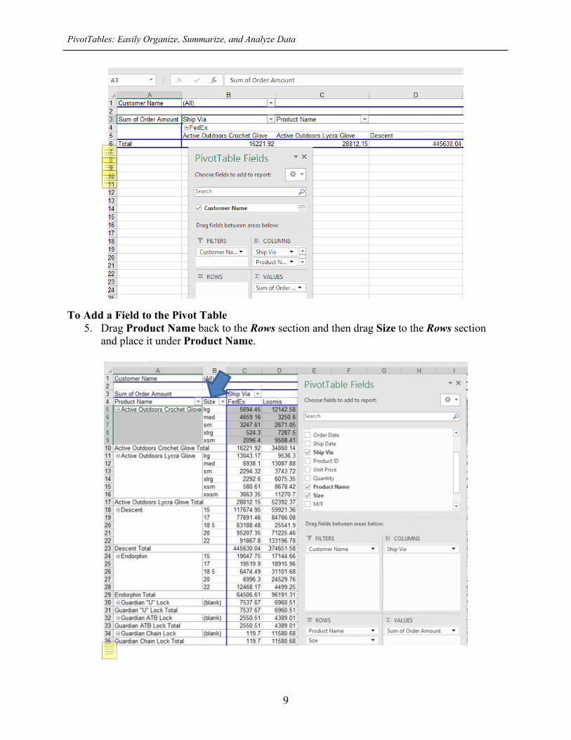
The Pivot Table now says Average Order Amount and the data now reflects the averages.

Formatting Calculations

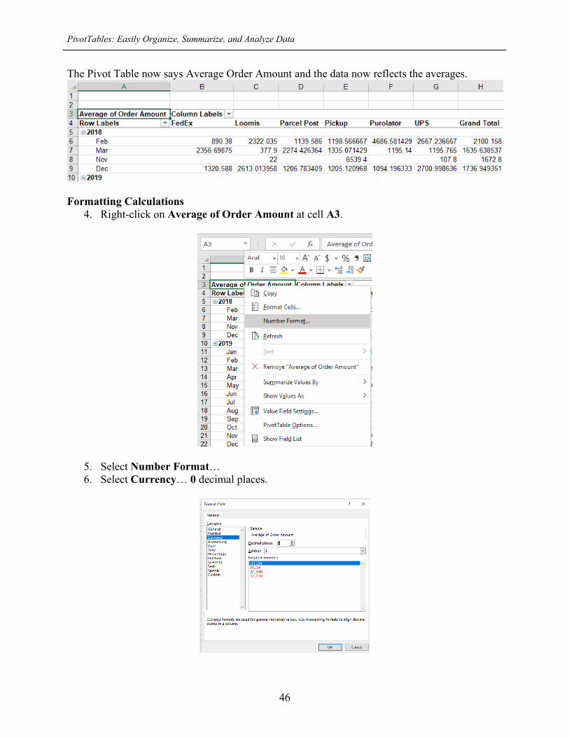
4. Right-click on Average of Order Amount at cell A3.

5. Select Number Format… 6. Select Currency… 0 decimal places.


47

7. Click OK.

The advantage of using the Pivot Table Format dialog box is that when you move, add data, or refresh in the Pivot Table, the formatting will still be applied. This is not true if you use the Ribbon formatting that you apply to cells. Subtotals and Totals Depending upon your data, Excel may include or exclude subtotals by default; however, you can control whether to add or remove subtotals and totals.

8. Make sure your cursor is in the pivot table. 9. Click on the contextual Design toolbar and click on the Subtotal icon. (Earlier versions

may find the Design icon on another contextual Pivot toolbar).


48

10. Select Show all Subtotals at Bottom of Group. We do not have any filtered items, but if you did, you would be able to specify if they should be included in the totals. You should now see totals for each year.

Totals If you click on the Grand Totals icon, you can see that you have a lot of options there as well.

Using Excel Preset Calculations Sometimes, numbers by themselves don’t tell the story. Excel offers some alternative ways to show the values. For example, percentages generally tell a more powerful story than just


49

numbers. Let’s take a look at ways to use percentages in the Pivot Table with minimal work on our part. Open Pivot_Value_Fields.xlsx and select Sheet 1.

At a glance, this Pivot Table does not seem to be very helpful. It’s hard to identify which shipper we use the most and which shipper we use the least. Let’s change it to a percentage and see if it is any clearer.


50

1. Right-click on Sum of Order Amount or one of the order amounts in the Pivot Table. 2. Select Show Values As.

3. Select % of Grand Total. Your Pivot Table should resemble the screenshot below:


51

Wasn’t that easy? As an added bonus, Excel is completing the calculations for you, which is quite nice. You could also right-click on one of the Order Amounts and sort by smallest to largest. Let’s see what else we can do.


52

Open Pivot_Value_Fields.xlsx and select Sheet 1 if necessary.

1. Right-click on Sum of Order Amount again. 2. Select Show Values As. 3. Select % Difference From. 4. Select Ship Via as your Base Field: 5. Select Loomis as your Base Item:

All the other Shippers will be compared against Loomis.

6. Click OK.

The Loomis row is blank as that is the base that everything is being compared against. The field must be in the Pivot Table in order for you to compare it. This comparison can be useful if you wanted to compare products or sales regions against each other. It is often easier to see trends with a percentage.


53

An alternate method is: 1. Right-click on the Pivot Table data and select Value Field Settings. 2. You can then select the Show Values As tab. 3. Click on the drop-down and select % Difference From or whatever else you want to

choose.

1. Click OK

Different Ways to Look at the Same Data Below are three Pivot Tables from the same data source that are presented differently. These custom calculations allow you to slice and dice the same data in multiple ways. In this example, sales are shown by product, by region, by sales dollar volume


54

In this example, sales are shown by percentages, by product, by region.

In this example, produce is being compared against dairy.

Create Calculated Fields within a Pivot Table Excel allows you to create a new calculated field in your Pivot Table which is based on calculations using existing fields in your table. Once created, it can be used in your table as if it were a data source. However, if you wish to use it in other tables, you must base your new table off the table with the calculation in it. In the example below, we have our list of customers with last year’s orders. In the following steps, we are going to create a new field named Commission and then use it in the Pivot Table.


55

Open Pivot_Calculated_Field.xlsx.

Excel 2013 users and earlier, please skip the next two steps and instead go to the steps for earlier versions. For newer versions, please do step 1 and 2 and then go to step 3.

1. Click on the contextual ribbon named PivotTable Analyze. 2. Click on the drop-down arrow beside the Fields, Items & Sets icon.

Step 1 and 2 for earlier versions:

1. Click on the contextual ribbon named Options 2. Click on the drop-down arrow beside the Fields, Items & Sets icon.

3. Click on Calculated Field…


56

A dialog box will display.

4. In the Name: field, type in Commission. 5. In the Formula: field, type or select Last Year’s Sales and then click Insert Field. 6. Type *10% in the Formula section

The example creates a new field name called Commission, which is calculated as 10% of Last Year’s Sales.

7. Click Add. 8. Click OK.

A new column named Commissions has been added to the existing Pivot Table, and the field has been added to the Pivot Table Fields pane, so it can be used in other calculations if need be.


57

Excel automatically includes the new field in the table for you.

Formulas for calculated fields operate on the sum of the underlying data for any fields in the formula. The formula does not multiply each individual sale by 10% and then sum the multiplied amounts. Tip: If you base a new Pivot Table on an existing table that has a calculated field, then you will see the calculated field on the Field Pivot Table pane as well.

Create a Calculated Item within a Pivot Table Excel allows you to create calculated items as well as calculated fields. When you first see this option, you may find it hard to imagine what you would do with it. However, it does have its uses. For example, you may want to consolidate products into a product line or perhaps you are merging a division or a department into another.


58

As you can see from the screenshot below, we have a lot of products and that makes the Pivot Table a bit unwieldy. It would be a simpler and easier to read the Pivot Table if we could simply roll the products up.

Let’s add all the Guardian products together and create a product line called Guardian Locks. We will be focusing on Column A, which is text, since we are in essence going to be adding text items together using the plus (+) symbol. Open Pivot_Calculated_Item.xlsx.

1. Click on a cell in Column A (Column A contains text). 2. Select the drop-down arrow under Fields, Items & Settings on the contextual ribbon.

3. Select Calculated Item… An Insert Calculated Item dialog box displays


59

4. In the Name: section, type over Formula1 and replace it with Guardian Locks. 5. In the Formula: section, select the 0 to overwrite it and then click on Guardian “U”

lock in the Items: list. 6. Click Insert Item. 7. Type + . 8. Click on the next Guardian item (Guardian ATB Lock) and then click Insert Item.

9. Continue until all 5 of the Guardian items are selected.


60

10. Click OK.

If you click on the filter icon of Product Name at cell A3 and scroll all the way down, you will now see Guardian Locks as the last item on the list.

If you deselect all other items except for Guardian Locks, the following displays:


61

This is a summary of the order amount for all of the Guardian Lock products. You could do this for all the other product lines if you wanted to nicely display a summarized Pivot Table. Modifying/Deleting Calculated Fields and Items. If you wish to delete or modify a calculated item or field, go back to the Calculated Item dialog box and then click the drop-down arrow beside Name: to access the calculated field. Once it is selected, you can modify or delete it.

Formula List If you’ve used calculated items and calculated fields in your Pivot Tables, you can create a list of all the formulas to keep track of them.


62

1. Click the drop-down arrow on the Fields, Items & Settings icon. 2. Select List Formulas.

Excel will display all calculated fields and items on a new sheet in the workbook.

Auto Formatting a Pivot Table Excel offers a variety of formatting options. You can easily format your Pivot Table using the contextual Design Ribbon. Excel also offers a number of predefined Pivot Table Styles. If you elect to use the predefined styles, add them at the very end as sometimes the styles will move your data around a bit or they will make formatting the Pivot Table more difficult. Click on the contextual Design tab to see your choices. They do differ slightly depending upon your version of Excel.


63

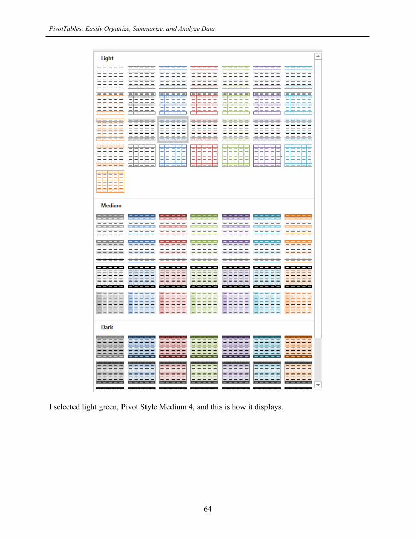
If you click the arrows at the end of the PivotTable Styles section, you can scroll through and see designs using the scroll buttons or click on the bottom button (More) to display the entire gallery of styles.


64

I selected light green, Pivot Style Medium 4, and this is how it displays.


65

PivotTable Styles Gallery You can further change your table’s formatting by selecting options such as:

• Hiding or displaying the header row • Displaying Banded Rows or Banded Columns, in which the even rows or Columns are

formatted differently from the odd rows and columns, much like the old accounting greenbar report

• Displaying subtotals and grand totals • Modifying the report layout.

To remove a Pivot Table style

1. Display the Pivot Table Style gallery. 2. Choose Clear from the bottom of the dialog box.

3. The PivotTable will display in the default format.

To Format a PivotTable

1. Click anywhere within the PivotTable to select it. 2. Click the contextual Design Ribbon.


66

3. Click the More button on the PivotTable Styles group to see the gallery of available styles. Tip: You can preview a style by moving your cursor over the styles.

4. Click the style that you want.

To Format individual parts of the PivotTable 1. Click anywhere within the PivotTable to select it. 2. Click the contextual Design Ribbon (under Table Tools). 3. On the PivotTable Style Options group, do one of the following:

• To turn the header rows on or off, select or clear the Row Headers or Columns Headers check box.

• To display odd and even rows with different formatting, select the Banded Rows check box.

• To display odd and even Columns with different formatting, select the Banded Columns check box.

• Click the Report Layout button to change the report layout to compact, outline or tabular.

• To insert or remove a blank row after each item, click the Blank Row button.

Remember—if you do not see a contextual toolbar then your cursor is not in the Pivot Table. Open Pivot_Format.xlsx and select Sheet 1.

1. Click on a cell in the Pivot Table. 2. Click the contextual Design tab. (If you can’t see it, make sure that your cursor is in the

Pivot Table) 3. Scroll through the gallery of PivotTable Syles and select Light green, Pivot Style Medium

25. Put a checkmark in the Banded Row box.

Excel will apply formatting to every other row. Depending upon your version, your worksheet may look slightly different than the screen shot below.


67

The banded rows definitely help make a long Pivot Table more readable. Try clicking on Banded Columns and see the difference.


68

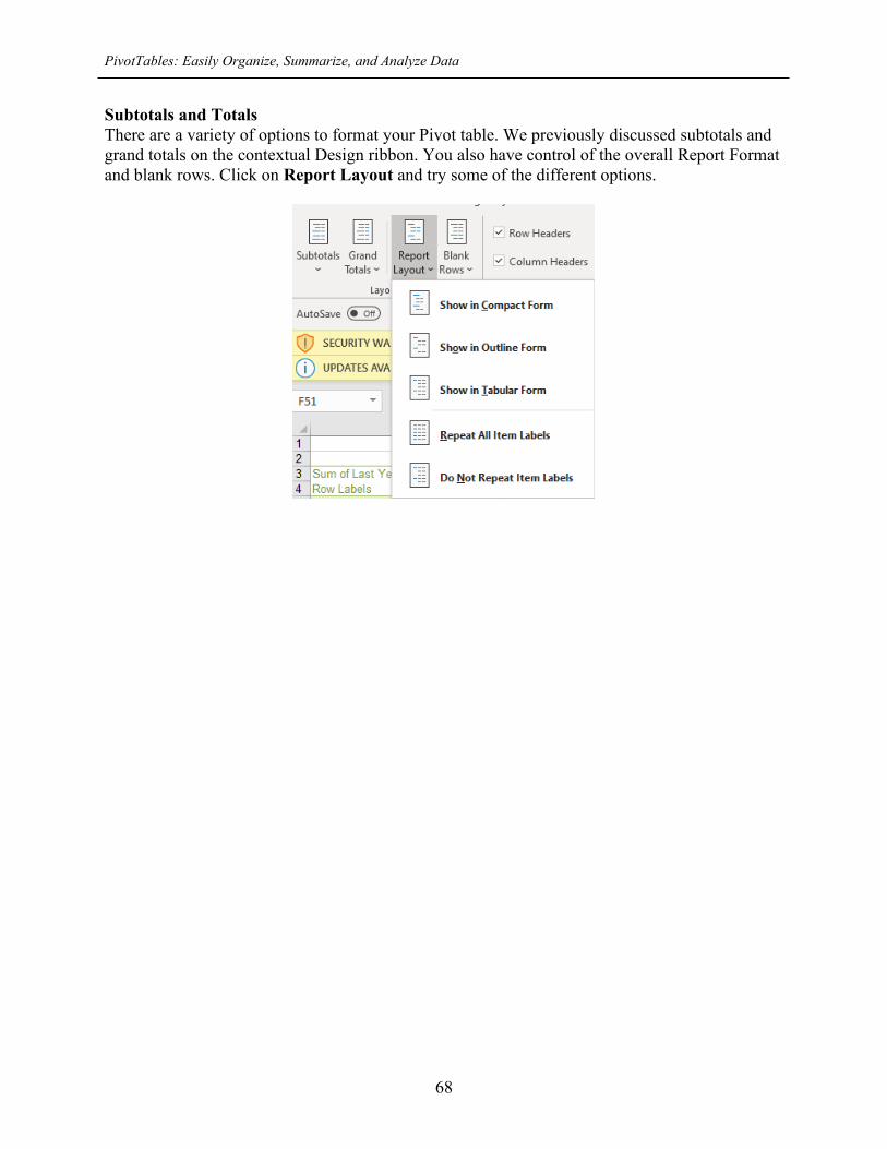
Subtotals and Totals There are a variety of options to format your Pivot table. We previously discussed subtotals and grand totals on the contextual Design ribbon. You also have control of the overall Report Format and blank rows. Click on Report Layout and try some of the different options.

Review Questions

69

Review Questions The review questions accompanying this course are designed to assist you in achieving the course learning objectives. The review section is not graded; do not submit it in place of your qualified assessment. While completing the review questions, it may be helpful to study any unfamiliar terms in the glossary in addition to course content. After completing the review questions, proceed to the review question answers and rationales. 7. When you create a new calculation in a Pivot Table, the field displays automatically in

the: a. Pivot Table Fields Pane. b. In the Column section. c. In the Row section. d. It does not automatically display anywhere.

8. To quickly make a Pivot Table “look pretty,” use the:

a. Report Layout command. b. Pivot Table Styles. c. Blank Rows icon. d. Quick Format button.


70

Pivot Table Charts A Pivot Chart is just as flexible as a PivotTable and can be arranged to organize your data in any manner you wish. A PivotChart report changes if you change the underlying PivotTable report and vice versa, as the chart is based on the underlying Pivot Table. You can format your PivotChart (chart type, chart options, etc.) just as you would a standard chart. Best of all, you can generate a PivotChart very easily. Having said all of that, let me add this caveat. Pivot Tables have a lot of data, and often your data is not going to be summarized down to a level appropriate for a chart. In other words, if your data is not summarized well, a Pivot Chart is not going to be very useful. Certain chart types such as scatter, bubble, and stock charts cannot be made from a Pivot Table. In Excel 2016, you can create a Pivot Chart directly from your data or from the Pivot Table itself. Let’s take a look at how to create one by selecting the data. Creating a Pivot Chart from Excel Data Open Pivot_chart.xlsx and select the sheet named Data.

1. Click in your data and then select the Insert menu. 2. Double-click on the PivotChart icon or click the drop-down arrow under the icon select

Pivot Chart.

3. Double-check the data range and location and click OK.


71

A PivotChart Field pane appears as does a chart layout and a Pivot Table Layout.

4. Click and drag Last Year’s Sales to the Value section and Product Name to the Axis

category.


72

A chart will display similar to the one below.

A Pivot Chart is interactive and can be useful in a presentation. If you look at the Pivot Chart, you will see that Product Name has a drop-down so you can actually click in the chart and display or exclude different products. If you had “rolled items up” into calculated items, as we did earlier, you could display the calculated items or all of the separate items.

In some Excel versions, you can double-click on the Sum of Sales and change it immediately to Average or another function. Or you may have to right-click and then select Value Field Settings.


73

When I clicked on the Product Name drop-down and selected just Guardian products, the chart becomes a little more useful.

Creating a Pivot Chart from a Pivot Table If you have created a Pivot Table and then decide a Pivot Chart would be helpful, you can create one directly from the Pivot Table itself.

1. Simply click in the Pivot Table. 2. Click on the PivotTable Analyze contextual toolbar and select PivotChart.


74

You can also take a look at Recommended PivotTables to see some different formats.

Pivot Charts in earlier Excel versions (Excel 2013 or earlier)

1. Select a single cell in your data. 2. Click on the Insert Ribbon and click the drop-down arrow under PivotTable.

3. Select PivotChart. 4. Specify the location of the PivotChart and click OK.

A blank pivot chart is created and the PivotTable Field appears. 5. Move the fields to your desired location in the chart.

When you create a chart from the Pivot Table, Excel does all the work. It automatically creates your chart and uses the layout of the Pivot Table Report to determine the placement of fields. Row fields in the table become category fields (X axis) in the Pivot Chart Report, and column fields in the table become series fields (Y axis) in the chart. When you create a PivotChart, you will notice that there is an additional contextual toolbar that pops up. The Format tab allows you to insert shapes and to format shapes. The Design tab allows you to change chart type as well as select different Chart Styles. The Design tab


75

The Format tab

Review Questions

76

Review Questions The review questions accompanying this course are designed to assist you in achieving the course learning objectives. The review section is not graded; do not submit it in place of your qualified assessment. While completing the review questions, it may be helpful to study any unfamiliar terms in the glossary in addition to course content. After completing the review questions, proceed to the review question answers and rationales. 9. If you are creating a PivotChart from a PivotTable, you will need to select the PivotChart

icon from the _______ contextual toolbar. a. PivotChart icon b. 3D Map icon c. Pivot icon d. Column chart icon


77

Options Pivot Tables have a variety of options you can change.

1. Click in a Pivot Table and then click the Options icon.

2. Select Options and a PivotTable Options dialog box appears. (An alternative method is to right-click on the pivot table and select PivotTable Options.

There are a lot of options (no pun intended) in this dialog box. You can change the Layout and Format and specify how many empty cells and error values to display. The default is for grand totals; however, if you don’t like that, you can change it on the Totals & Filters tab. If you are old school and like the old classic Pivot Table style, you can find that under the Display tab.


78

The Data tab is very important.

The default is that the source data is saved with the Pivot Table in a pivot cache. So, even if you move or copy the sheet to another file, please keep in mind that all of the supporting data is there. This is of particular importance if you are emailing a pivot table to someone else. You can also specify if you want the table to be refreshed or updated whenever you open it, or you may view the table in its most recent form without updates. If you do not save the Source Data your file will be smaller and will need to be refreshed after opening the file. In addition, you can also change the Pivot Table Name, which is useful if you have multiple pivot tables in one file or if you want to reference the pivot table in a formula. Data Source If you are moving Pivot Tables and/or data around or using someone else’s Pivot Tables, you may need to locate the data source.

1. Click on a cell in a Pivot Table. 2. On the contextual ribbon, click the Change Data Source drop-down. If you have an

earlier version, you may need to click on the Options contextual toolbar and then select the Change Data Source icon.


79

3. Click Change Data Source and the following dialog box will display.

In this example, it is showing that the data is actually on another worksheet named Data. The actual source data will display behind the dialog box if the file is open. In the screenshot below, I had saved the pivot table in a new file and when I clicked Change Data Source, it displayed the location and name of the file where the source data is located.

Automatically Update a Pivot Table with New Data What happens when additional data is added to the source data? First, changes to the existing data are automatically updated when you select the Refresh button located on the contextual ribbon.

If you add additional rows of data, Excel does not automatically add that information to the Pivot Table. If it a static range, it will only continue to reference those specific cells.


80

However, it is easy to set it up so that Excel automatically updates the Pivot Table for any additional data. Starting with Excel 2010, you can turn your data into a table. If you do this, Excel will automatically update the Pivot Table. This is by far the easiest way to keep your table up to date. Create a Table Let’s turn a data list into a table so that it displays alternating row shading and AutoFilter drop down boxes.

1. Click in the data. 2. Click the Insert tab. 3. Click Table. 4. Verify the data range and click OK.

Excel now considers the data to be a table and it will incorporate new rows and columns of information as they are added. If you open your Pivot Table and re-select your data source, the Pivot Table will update as the range changes. As data is added, it will automatically be incorporated into the parameters of the original source data. If you don’t control the data, then you may not be able to turn it into a table. In that case, the process is a bit more involved as you need to create a dynamic range. It is definitely worth the effort. Create a Dynamic Range

1. Click in the source data. 2. Select the Formulas tab and click on Define Name. 3. In the New Name dialog box, name your data. In the screenshot below, I named the data

sales_data.

4. The Scope: field should stay at the default level of Workbook. 5. In the Refers to: section, type the following:

=OFFSET(Sheet1!$A$1,0,0,COUNTA(Sheet1!$A:$A),COUNTA(Sheet1!$1:$1)) 6. Click OK.


81

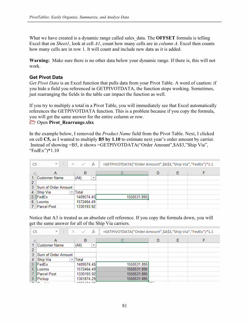
What we have created is a dynamic range called sales_data. The OFFSET formula is telling Excel that on Sheet1, look at cell A1, count how many cells are in column A. Excel then counts how many cells are in row 1. It will count and include new data as it is added. Warning: Make sure there is no other data below your dynamic range. If there is, this will not work. Get Pivot Data Get Pivot Data is an Excel function that pulls data from your Pivot Table. A word of caution: if you hide a field you referenced in GETPIVOTDATA, the function stops working. Sometimes, just rearranging the fields in the table can impact the function as well. If you try to multiply a total in a Pivot Table, you will immediately see that Excel automatically references the GETPIVOTDATA function. This is a problem because if you copy the formula, you will get the same answer for the entire column or row. Open Pivot_Rearrange.xlsx In the example below, I removed the Product Name field from the Pivot Table. Next, I clicked on cell C5, as I wanted to multiply B5 by 1.10 to estimate next year’s order amount by carrier. Instead of showing =B5, it shows =GETPIVOTDATA(“Order Amount”,$A$3,”Ship Via”, “FedEx”)*1.10

Notice that A3 is treated as an absolute cell reference. If you copy the formula down, you will get the same answer for all of the Ship Via carriers.


82

As a workaround, you can copy and paste the pivot table into another workbook if you want to do any math on the Pivot Table. However, the following is a great tip from the MrExcel.com website on how to avoid this problem.

1. Go up the Options icon and click the drop-down arrow to the right. 2. Uncheck Generate GetPivotData.

If you go back to cell C5 and recreate the formula, you will see the formula bar shows =B5*1.10. It will now copy down correctly. (Excel will not correct the GETPIVOTDATA formula, so you need to delete it and then type in =B5*1.1.)

The best part is that once you uncheck Generate GetPivotData, Excel remembers so you do not have to keep unchecking the icon every time you want to use a formula that references the pivot table.

Debra Dylan

CHECK FOR ACCURACY.

Review Questions

83

Review Questions The review questions accompanying this course are designed to assist you in achieving the course learning objectives. The review section is not graded; do not submit it in place of your qualified assessment. While completing the review questions, it may be helpful to study any unfamiliar terms in the glossary in addition to course content. After completing the review questions, proceed to the review question answers and rationales. 10. The _______ tab allows you to select and change the chart type.

a. Layout. b. Design. c. Format. d. Analyze.

11. Which of the following defaults can you change on a Pivot Table?

a. Change the color of Pivot Table to dark blue. b. Change font size. c. Print data and PivotTable together automatically. d. Tell Excel to refresh data when file is opened.

12. If you want to have your chart update automatically as data is entered into it, use the

_______ in conjunction with the OFFSET function. a. COUNT. b. COUNTA. c. COUNTIF. d. COUNTBLANK.


84

Review/Feedback Exercise Open Pivot_Table_on_your_own.xlsx.

1. Click on the Sales Info worksheet. 2. Create a PivotTable from the sales data list and place the PivotTable in a new worksheet. 3. Add Salesperson to the Report filter area. 4. Add Month Ending to the Row section. 5. Add Product Line to the Column section. 6. Add Sales Volume to the Values section. 7. Change the function so that the table displays Average Sales Volume. 8. Format the data so that it displays as Number or as currency with 0 decimals. 9. Filter Category so that Video Games does not display. 10. Create a PivotChart from the Pivot Table using the Column default. 11. Change the chart so that it only displays Susie Loftus instead of all salespeople. 12. Save the file.

If you wish to compare your answers, reference Pivot_Table_on_your_own_answer.xlsx. Review/Feedback Answers

1. Click in the data and go to the Insert ribbon. Select the PivotTable icon’s drop-down arrow and then select PivotTable.

2. Drag Salesperson, Month Ending, Product Line, and Sales Volume to the appropriate places in the PivotTable Fields pane.

Your worksheet should resemble the one below. You can also reference it in Pivot_Table_on_your_own_answer.xlsx.


85

3. Right-click on the Sum of Sales Volume>Summarize Values by and select Average.

4. Right-click on the sales volume number in cell A3 and select Number format (there are several ways to do this.)

5. Click the drop down arrow beside Product Line (Column Labels) in the pivot table and remove the checkmark from Video Games.


86

6. Click the PivotChart icon on the contextual toolbar to create a PivotChart (columni chart

is the default) and have it display just for the salesperson named Susie Loftus.

Review Question Answers and Rationales

87

Review Question Answers and Rationales Review question answer choices are accompanied by unique, logical reasoning (rationales) as to why an answer is correct or incorrect. Evaluative feedback to incorrect responses and reinforcement feedback to correct responses are both provided. 1. When creating a Pivot Table, numeric fields such as Unit Sales or Order Amount should

be dragged to the _______ area. a. Filters. Incorrect. Unit Sales, if displayed in the Filters section, would not provide

useful information and the sales could not be summarized. b. Columns. Incorrect. Columns are designed for text or date fields. A field such as Unit

Sales could create a massive Pivot Table, as the data could not be summarized well. c. Rows. Incorrect. Rows are designed for text or date fields, and a number field, such

as Unit Sales, would not be summarized well. d. Values. Correct. The Values area allows numbers to be summarized and a total

to be displayed 2. Which of the following statements is FALSE?

a. When creating a Pivot Table, the source of the data displayed can be an existing

worksheet of data. Incorrect. This is true statement. A Pivot Table can be based upon existing data in an Excel worksheet.

b. When creating a Pivot Table, data can be imported from an external source. Incorrect. This is a true statement. A Pivot Table’s data source can be from external sources such as Access or QuickBooks.

c. When creating a Pivot Table, the Pivot Table by default is placed in a new file. Correct. This statement is false. The default for Pivot Table creation is in an existing worksheet, not a new file.

d. When creating a Pivot Table in Excel 2013 and higher, the Pivot Table by default is placed in a new worksheet. Incorrect. This statement is true. The default location for a Pivot Table in Excel 2013 and higher is in a new worksheet.

3. If you had the following fields, Salesperson, Region, and Unit Sales, and wanted to

display information by different Regions, where would you place that field? a. Filters. Correct. The Filters essentially controls the data as it summarizes the

values by whatever field is displayed the report filter. b. Columns. Incorrect. The Columns area displays data but does not control what is

summarized c. Rows. Incorrect. The Rows area displays data but does not control what is

summarized. d. Values. Incorrect. The Values field is where values are displayed and summarized but

it does not control what data displays.


88

4. Excel introduced buttons called _______ where a user can click to filter the PivotTable data and the filtered information remains visible on the worksheet. a. Oranges. Incorrect. Oranges are a fruit. b. Slicers. Correct. Slicers were introduced in Excel 2010 so that when a user filters

data in a Pivot Table, they can see what was actually filtered. c. Peelers. Incorrect. Peelers are a kitchen utensil used to peel fruit. d. Filters. Incorrect. Filters hide data and they do not remain visible in the worksheet.

Filters have also existed in earlier versions of Excel.

5. You have a workbook that contains 2 sheets. One sheet contains all your data for 4 sales regions, and the other contains a Pivot Table as shown below. If you select the Show Report Filter, how many additional pages would be added to the file?

a. 0. Incorrect. You have regions on the Report Filter so region information would display if you selected Show Report Filter Pages.

b. 3. Incorrect. If B1 had displayed a region such as East, then this 3 would be correct, but since it displays All, this is not the correct answer.

c. 4. Correct. Since B1 shows All, Excel would display a detail page for each of the 4 regions.

d. 5. Incorrect. Excel can only display available data. Since there are only 4 regions of data, only 4 regions or less can display.

6. To display individual products as a product line in your Pivot Table, select: a. Group. Correct. The Group command allows you to combine fields and display

as a single entity in the Pivot Table. b. Merge. Incorrect. Excel does not offer a command called Merge. c. Summarize Values As. Incorrect. Summarize Values As allows you to do

mathematical calculations on values. It does not allow you to group fields together. d. Refresh. Incorrect. Refresh merely updates the data in the existing Pivot Table.


89

7. When you create a new calculation in a Pivot Table, the field displays automatically in the: a. Pivot Table Field Pane. Correct. When you create a new calculation in a Pivot

Table, it automatically displays in the Pivot Table and on the Pivot Table Field Pane.

b. In the Column section. Incorrect. The field does not automatically display in the Column section – you would have to drag it to the column area manually.

c. In the Row section. Incorrect. The field does not automatically display in the Row section – you would have to drag it there manually.

d. It does not automatically display anywhere. Incorrect. The field automatically displays in the Pivot Table itself as well as the Pivot Table Field Pane.

8. To quickly make a Pivot Table “look pretty,” use the:

a. Report Layout command. Incorrect. The Report Layout changes the display of the

Pivot Table report. It does not format. b. Pivot Table Styles. Correct. The Pivot Table Style feature allows you to select a

style, and Excel will then do all the formatting, such as color and fonts, based upon the style you chose.

c. Blank Rows icon. Incorrect. The Blank Row icon just creates blank rows, which may make the report more readable, but it does not make it prettier.

d. Quick Format button. Incorrect. Excel does not offer a Quick Format button.

9. If you are creating a PivotChart from a PivotTable, you will need to select the PivotChart icon from the _______ contextual toolbar. a. PivotChart icon. Correct. The Pivot chart icon is located on the contextual

toolbar and allows you to create a Pivot Chart. b. 3D Map icon. Incorrect. The 3D Map does not allow you to create a PivotChart. c. Pivot icon. Incorrect. There is no Pivot icon in Excel. d. Column chart icon. Incorrect. A column chart does not create a PivotChart. A

column chart will not allow you to have the drop-down interfaces that the PivotChart allows you.

10. The _______ tab allows you to select and change the chart type.

a. Layout. Incorrect. The Layout tab allows you to add items such as trend lines and to

document, but it does not allow you to change the chart type. b. Design. Correct. The Design tab allows you to change the chart type of the pivot

chart. c. Format. Incorrect. The Format tab, as the name says, allows you to change formatting

features such as color or font size; however, it does not allow you to change the chart type

d. Analyze. Incorrect. The Analyze tab allows you to do things such as add slicers; however, it does not allow you to change the chart type.


90

11. Which of the following defaults can you change on a Pivot Table?

a. Change the color of Pivot Table to dark blue. Incorrect. The color of a Pivot Table

cannot be changed by default. b. Change font size. Incorrect. A Pivot Table has a standardized font size that cannot be

changed by default. c. Print data and Pivot Table together automatically. Incorrect. Data and the Pivot Table

do not automatically print together if they are on separate pages and this cannot be changed as a default.

d. Tell Excel to refresh data when the file is opened. Correct. Excel’s default is that data is not automatically refreshed when the workbook is open; however, you can change this default in the Options section.

12. If you want to have your chart update automatically as data is entered into it, you should

use the ___________ in conjunction with the OFFSET function. a. COUNT. Incorrect. COUNT would be correct, but only if you are counting numbers.

It is not the best answer available. b. COUNTA. Correct. COUNTA counts both numbers and text so you would be

sure that Excel is accounting for all new data entered. c. COUNTIF. Incorrect. The COUNTIF function only counts data if a certain condition

is set. This will not work with OFFSET to automatically include all data entered into the chart.

d. COUNTBLANK. Incorrect. COUNTBLANK counts blank cells and would not be helpful in updating a chart for new data automatically.

Glossary

91

Glossary This is a glossary of key terms with definitions. Please review any terms with which you are not familiar. Pivot Chart: A graphical representation of a Pivot Table. Pivot Table: A data summarization tool. Among other functions, pivot table tools can automatically sort, count, total, or give the average of the data stored in one table or spreadsheet. It displays the results in a second table (called a "Pivot Table") showing the summarized data.1 Refresh: A method used to connect to the source data and the update function. Slicer: A visual control or button that allows the user to quickly filter data. A slicer floats above the worksheet is visible. In addition, a slicer allows the user to filter fields not actually displayed in the Pivot Table. Source Data: Underlying numbers or foundation.

1 Wikipedia

Index

92

Index A

automatically updated .............................................. 79

C

calculated field ................................................... 54, 57 calculated items ........................................... 57, 61, 95 Calculations ............................................................. 45 Column Labels ........................................................... 8 Control key ....................................................... 21, 39 COUNTA ................................................................ 80

D

data source ......................................................... 54, 78 dates ......................................................................... 35 default function ........................................................ 45 Design ......................................................... 62, 65, 66 Drilling Down .......................................................... 26 dynamic range ......................................................... 81

F

Field List task pane ............................................ 57, 84 Fields, Items & Settings ........................................... 58 filter ................................................. 13, 14, 42, 43, 84 filter your fields ...................................................... 13 formatting .............................................. 47, 62, 65, 66 Formula .................................................................. 56 formulas .................................................................. 13 function .................................................................... 45

G

Group ........................................................... 31, 39, 43 Grouping .......................................... 23, 30, 33, 35, 39

L

List Formulas ......................................................... 62

O

OFFSET.................................................................. 80

P

Pivot Chart ......................................................... 70, 74 PivotTable Field List ..................................... 1, 5, 6, 7 preset calculations.................................................... 48

R

Refresh ................................................................. 1, 93 Report Filter .......................................................... 5, 6 Review ......................................................... 33, 42, 84

S

Show Report Filter Pages .......................... 29, 44, 96 Slicers ................................................................ 18, 91 sort ............................................................... 13, 24, 43 Sort ........................................................ 24, 25, 43, 94 sort order .................................................... 13, 24, 43 Subtotals .................................................................. 68 Sum of Sales ............................................... 45, 46, 52

T

Table Styles removing ............................................................. 65

Totals ....................................................................... 68

U

Ungroup ....................................................... 32, 33, 42

V

value field ................................................................ 95 Value Field .................................................. 45, 53, 94 Values ..................................................................... 45

Debra Dylan

CHECK FOR ACCURACY.

Qualified Assessment

93

Qualified Assessment PivotTables: Easily Organize, Summarize and Analyze Data

Course # 2164542, Version 2007 Publication/Revision Date:

July 2020 Course Expiration Date Per AICPA and NASBA Standards (S9-06), QAS Self-Study courses must include an expiration date that is no longer than one year from the date of purchase or enrollment. Complete this assessment online at www.westerncpe.com and receive your certificate and results instantly! 1. Which of the following is NOT a true statement?

a. Pivot Tables allow you to analyze complex data. b. The data in a Pivot Table is read-only. c. Once you have created a Pivot Table, you can refresh the data (from the Ribbon). d. Pivot Tables are extremely difficult to create.

2. To create a Pivot Table, click the _______ tab on the ribbon.

a. Create. b. Insert. c. Design. d. Pivot.

3. Pivot Tables by default will be placed

a. In a new worksheet. b. In a new workbook. c. In an existing worksheet. d. In a new file.

4. Which of the following is a part or section of a Pivot Table Field pane?

a. Corners. b. Squares. c. Variances. d. Filters.

5. Which of the following is NOT a true statement? a. You can rearrange data by right-clicking on a field name in the Pivot Table. b. You can rearrange data by dragging a field name onto the Pivot Table. c. The PivotTable Fields pane is always visible. d. Fields in the Pivot Table can be sorted.



94

6. The _______ is extremely important as it controls all of the other data. a. Filters section. b. Value section. c. Rows section. d. Data section.

7. To see the PivotTable Fields pane, the cursor needs to be:

a. In the source data. b. In the Pivot Table. c. Anywhere in the worksheet. d. Anywhere in the file.

8. To create a Pivot Table that displays both total and average sales, you will need to:

a. Create a slicer to display the average. b. Drag the Sales field into the Pivot Table Value field twice and change one of the

Value Fields to Average. c. Click on the rearrange button in the Pivot Table. d. Create a calculation using the AVERAGE function.

9. Which of the following statements is True?

a. When you hide a field in the Pivot Table, the total excludes the hidden field. b. You can only hide multiple fields. c. If you use a custom sort, the sort order is retained when the data refreshes, if set to

manual. d. You can only sort data in a Pivot Table in ascending order.

10. Slicers: a. Can be resized and formatted. b. Display in green. c. Are shaped as ovals. d. Are orange.

11. Which of the following statements about sorting is FALSE?

a. You can sort field names in a Pivot Table by clicking on the Sort icon. b. You can sort field names by right-clicking and selecting sort. c. You can manually sort by clicking field names and dragging them. d. You can sort fields by color.


95

12. Which of the following statements is FALSE? a. You can rename a field name simply by clicking on it and typing over it. b. The only way to remove a field from a Pivot Table is by dragging it off the Pivot

Table. c. Dates cannot be grouped in a Pivot Table. d. You can right-click on the value field and change the function from Sum to Average.

13. To drill down and have summary information display

a. Click on the Drill Down icon found on the Pivot Table ribbon. b. Click the Report Layout icon on the Layout group of the Pivot Table ribbon. c. Double-click on the detail in the Pivot Table. d. Click on the Summary button.

14. Which of the following statements about formatting is FALSE?

a. When you select Banded Rows on the Design ribbon, the Pivot Table will display odd

and even rows with different formatting to make the data more readable. b. You can change Pivot Table numbers to display as percentages. c. Pivot Table number formatting remains when data is refreshed if you used the Format

dialog box on the Home ribbon. d. When you select Banded Column on the Design ribbon, the Pivot Table will display

odd and even Columns with different formatting to make the data more readable. 15. To keep track of calculated items and calculated fields in your Pivot Table, you can

create a list of formulas to keep track of them. To do so, select _______ from the Calculations icon on the contextual toolbar. a. List Calculations. b. List Formulas. c. Track Calculations. d. Track Formulas.

16. Which of the following statements about PivotCharts is TRUE?

a. You can create a PivotChart from either a PivotTable or data in a worksheet. b. You can create a bubble chart Pivot Chart. c. The more data you have the more useful a PivotChart becomes. d. A Pivot Chart is static – it never refreshes.


96

17. Which of the following statements is TRUE? a. When you create a new field such as Commission, that field will then display in the

PivotTable Field Pane. b. To turn a Header row on, clear the Columns Headers check box. c. If you place a checkmark in Banded Row, all row formatting disappears. d. If you place a checkmark in Banded Row, alternate Columns blue formatting appears.

18. To generate multiple reports from a Pivot Table:

a. Select the Show Report Filter. b. Double-click on the Filter icon. c. Click the filter icon and select Multiple Items. d. You cannot generate multiple reports.

19. A _______ chart can be made from a Pivot Table.

a. Line. b. Scatter. c. Bubble. d. Stock.

20. To locate the source of the underlying data of the Pivot Table:

a. Select Change Data Source. b. Double-click on a field. c. Select Find Data Source. d. Select Show Data Source.

21. To create a dynamic range, you can use the _______ function.

a. PIVOT. b. GETDATA. c. OFFSET. d. DYNAMIC.

22. To change the defaults of a Pivot Table you would need to select _______ tab.

a. Options. b. Design. c. View. d. Developer.


97

23. The Excel function that pulls data from your Pivot Table is called _______. a. GETPIVOTDATA. b. PULLPIVOTDATA. c. GENERATEPIVOTDATA. d. YANKPIVOTDATA.

24. One way to update your data in a Pivot Table is by: a. Clicking Refresh on the ribbon. b. Clicking Update. c. Clicking Find New Data on the ribbon. d. Right-clicking in the data and selecting Update.

25. The easiest way to have a Pivot Table automatically update as new data is added is to:

a. Turn data into a table. b. Turn data into a delimited file. c. Turn data into a chart. d. Turn data into an object.

Answer Sheet

98

Answer Sheet PivotTables: Easily Organize, Summarize and Analyze Data

Course # 2164542, Version 2007 5 CPE Credits

Date:

Name:

Phone:

Address:

City:

State:

Zip:

Fax:

E-mail*:

*E-mail address MUST be unique (not shared with another CPA) for Western CPE to grade your assessment

Name of purchaser (if other than person taking assessment):

If course was purchased as part of the MEGA TAX LIBRARY please include $4/credit for grading: VISA/MC/Discover/Amex # Exp.

Course expires 1 Year from date of purchase or

enrollment

Online Grading: visit www.westerncpe.com to complete your assessment online and receive your certificate of completion and results instantly.

1. ___ 6. ___ 11. ___ 16. ___ 21. ___

2. ___ 7. ___ 12. ___ 17. ___ 22. ___

3. ___ 8. ___ 13. ___ 18. ___ 23. ___

4. ___ 9. ___ 14. ___ 19. ___ 24. ___

5. ___ 10. ___ 15. ___ 20. ___ 25. ___


Course Evaluation

99

Course Evaluation PivotTables: Easily Organize, Summarize and Analyze Data

Course # 2164542, Version 2007

Thank you for taking the time to fill out this course and customer experience evaluation. Your responses help us to build better courses and maintain the highest levels of service. If you have comments not covered by this evaluation, or need immediate assistance, please contact us at 800.822.4194 or [email protected]. Course and Instructor Evaluation 1. Please answer the following related to the content of the course: Strongly

Disagree Disagree Neutral Agree Strongly Agree

The stated learning objectives were met. O O O O O

The course materials were accurate, relevant, and contributed to the achievement of the learning objectives. O O O O O

The stated prerequisites were appropriate and sufficient. O O O O O

Based on 50 minutes per credit hour, the time to take this course accurately reflects the credit hours assigned to it. O O O O O

The instructor was knowledgeable and effective. O O O O O

2. Were there any questions you felt were confusing or had incorrect answers listed? If so, please give the question

number and a brief description of the issue:

3. Please provide any additional comments specific to the educational content or author of this course:

mailto:[email protected]

Course Evaluation

100

4. Do you have ideas for future course topics? If so, please list them along with any known subject matter experts we might contact to develop the course:

Customer Experience 5. Please rate your overall experience with Western CPE:

Unsatisfactory Improvement Needed

Meets Expectations

Exceeds Expectations Exceptional

If you interacted with our Customer Service team, please rate the quality of service you received.

O O O O O

If you purchased your course online, please rate the quality of your e-commerce experience.

O O O O O

“My Account” information includes the tools necessary to access courses and track those completed.

O O O O O

6. Please indicate the likelihood of your purchasing the listed course formats from Western CPE:

Not at all Not very likely Possibly Likely Highly

Likely

Self-Study O O O O O

Webcast OnDemand O O O O O

Live Webcast O O O O O

Resort Conference or Seminar O O O O O

Course Evaluation

101

7. Please use the box below to provide any additional comments related to your educational experience with Western CPE.

8. If you are willing to provide a quote about this course, or Western CPE in general, that we may use in our

promotional materials, please state it below. Be sure to include your name, title, city, and state.

Documents

PivotTables: Easily Organize, Summarize, and Analyze Data