Pit of Consumption…SAVINGS, CONSUMPTION AND REAL INCOME

Economics: the Dismal Science… based on assumptions…

• Assume businesses pay no indirect (sales) taxes

• Assume businesses distribute all of their profits to shareholders

• Assume there is no depreciation (gross investment = net investment)

• Assume economy is closed (no trade)

• This all is the basis of Real Disposable Income (RDI for short)

• RDI = Real GDP – taxes (direct)

Can only consume or save•Option of 2 things you can do with $1 of RDI:

•Consume now

•Save to consume later

What is consumption?•Using Income for purchasing consumption goods

•Consumption Goods: household immediate goods/services

Saving or Savings?

• FLOW= something that happens over time

• STOCK = certain point in time

• Saving: “rate” at which you put money away (flow)

• Savings: result of past saving ($1000 in the bank) (stock)

•Consumption is an example of flow

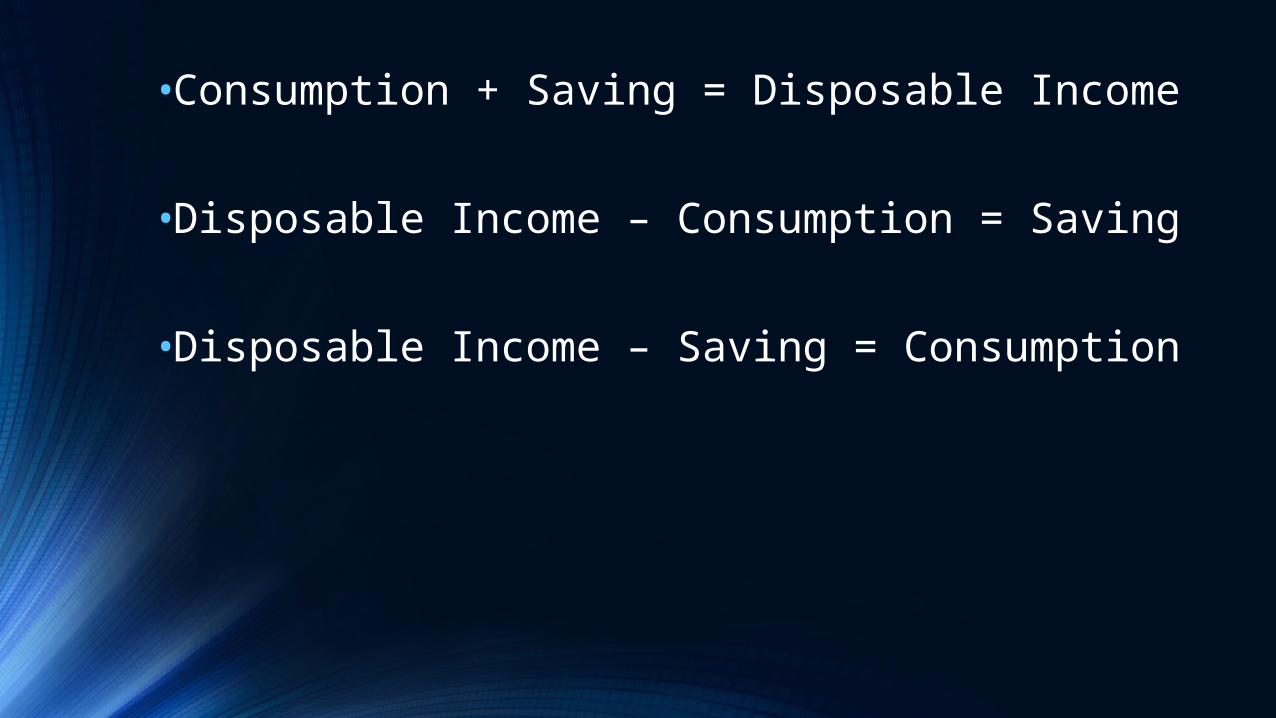
•Consumption + Saving = Disposable Income

•Disposable Income – Consumption = Saving

•Disposable Income – Saving = Consumption

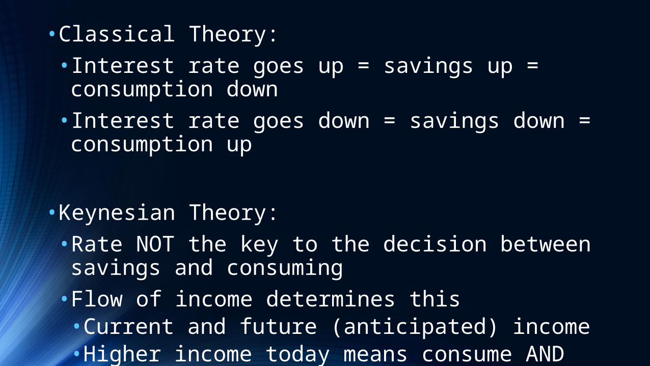
•Classical Theory: • Interest rate goes up = savings up = consumption down• Interest rate goes down = savings down = consumption up

• Keynesian Theory:• Rate NOT the key to the decision between savings and consuming• Flow of income determines this•Current and future (anticipated) income •Higher income today means consume AND save more•Anticipated income means consume and save more

•Consumption and Savings are compliments of one another

•Life-Cycle Theory of Consumption:• How a person varies consumption/savings over their lifetime• Anticipated income up = consumption up = savings up• Anticipated income down = consumption down = savings down

•Permanent Income Hypothesis:• Average Lifetime Income• Consumption only goes up if the average lifetime income goes up•A little change (or assumed temporary change) results in the same amount of consumption and saving the rest

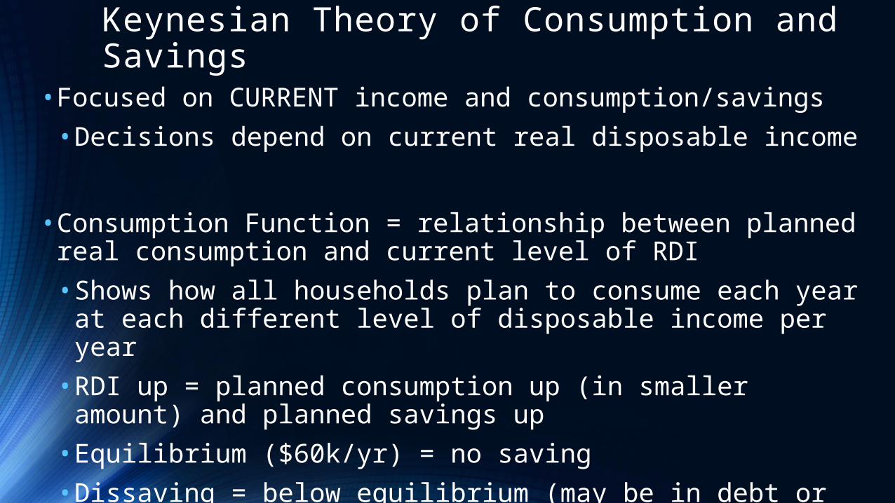
Keynesian Theory of Consumption and Savings

• Focused on CURRENT income and consumption/savings

• Decisions depend on current real disposable income

• Consumption Function = relationship between planned real consumption and current level of RDI

• Shows how all households plan to consume each year at each different level of disposable income per year

• RDI up = planned consumption up (in smaller amount) and planned savings up

• Equilibrium ($60k/yr) = no saving

• Dissaving = below equilibrium (may be in debt or using other wealth)

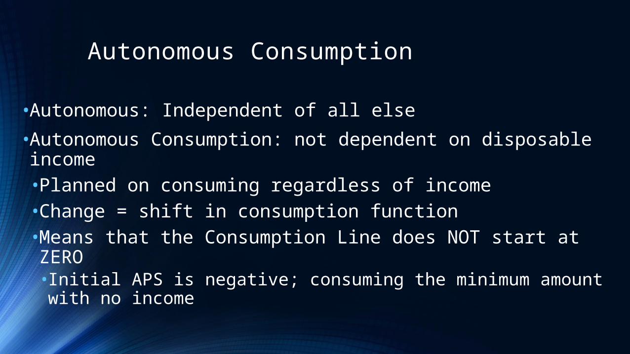
Autonomous Consumption

•Autonomous: Independent of all else

•Autonomous Consumption: not dependent on disposable income• Planned on consuming regardless of income•Change = shift in consumption function•Means that the Consumption Line does NOT start at ZERO• Initial APS is negative; consuming the minimum amount with no income

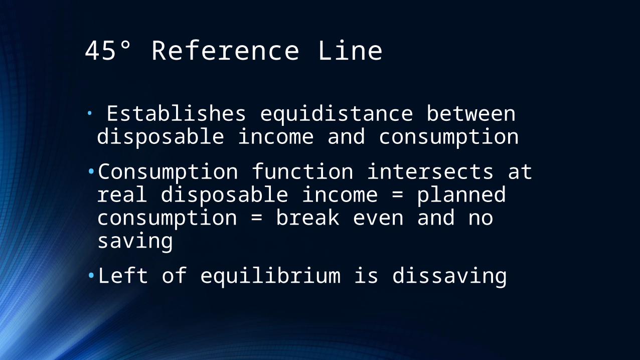
45° Reference Line

• Establishes equidistance between disposable income and consumption

•Consumption function intersects at real disposable income = planned consumption = break even and no saving

• Left of equilibrium is dissaving

Aggregate Expenditure = Consumption Function

• Total amount of real planned spending (consumption): C, I, G, NX

• Label of the vertical axis• NOT the same as the AD/AS where the vertical is price index

• Horizontal is Real GDP, not GDI

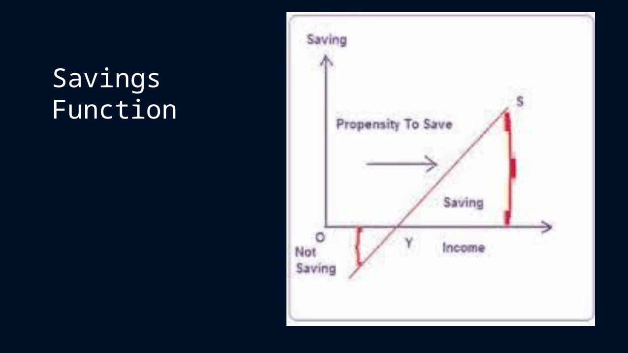
Savings Function

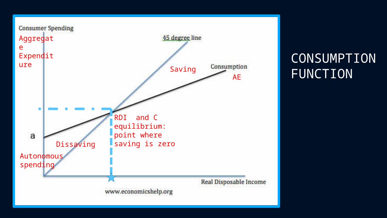
CONSUMPTION FUNCTIONSaving

Dissaving

Autonomous spending

RDI and C equilibrium: point where saving is zero

Aggregate Expenditure

AE

APC and APS

• Average Propensity to Consume = Real Consumption/Real Disposable Income• For any level of real income, proportion of total RDI that is consumed

• Average Propensity to Save = Real Saving/Real Disposable Income• For any level of real income, proportion of total RDI that is saved• Can be NEGATIVE (Dissavings)

• Based on average proportions: so as average propensity consumes decreases as income goes up. Average amount of income going toward consumption falls as income goes up. Average propensity to save will go up as income goes up because spending a smaller proportion, relative to higher income, on consumption

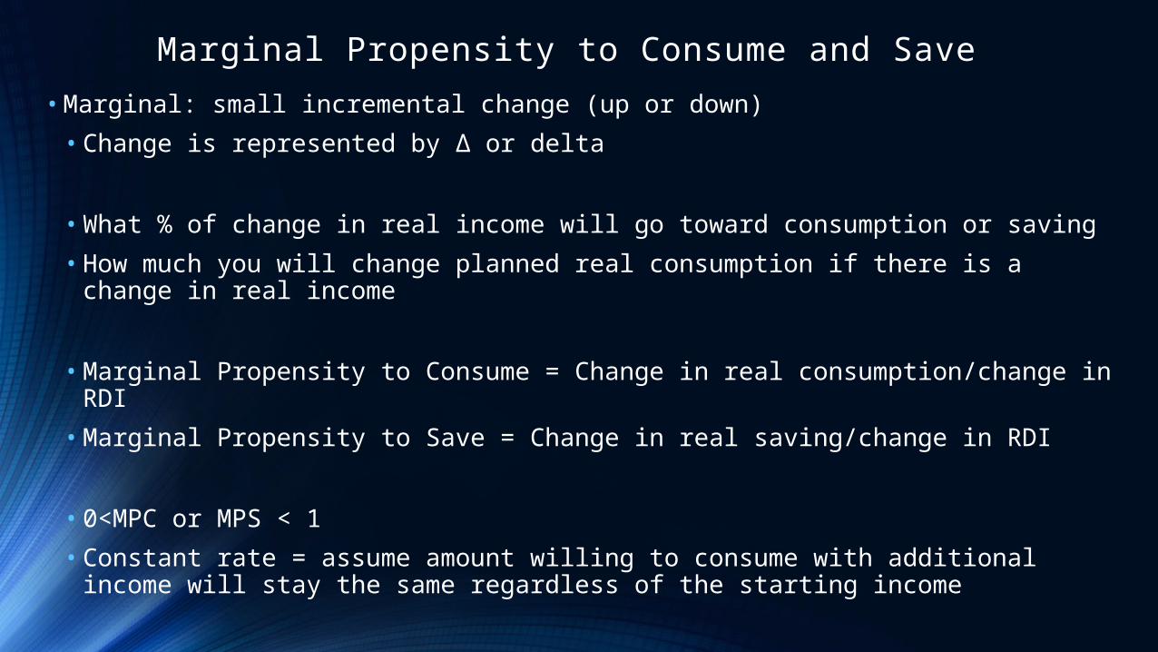
Marginal Propensity to Consume and Save• Marginal: small incremental change (up or down)

• Change is represented by Δ or delta

• What % of change in real income will go toward consumption or saving

• How much you will change planned real consumption if there is a change in real income

• Marginal Propensity to Consume = Change in real consumption/change in RDI

• Marginal Propensity to Save = Change in real saving/change in RDI

• 0<MPC or MPS < 1

• Constant rate = assume amount willing to consume with additional income will stay the same regardless of the starting income

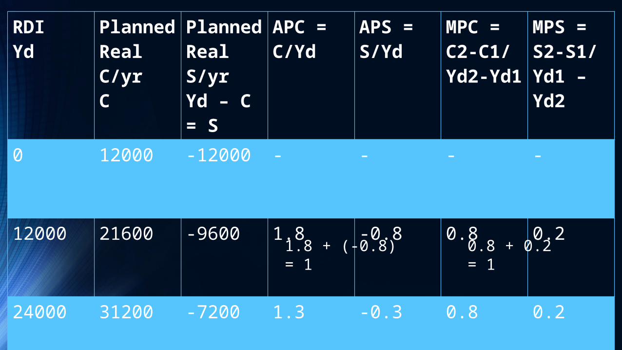
RDIYd

Planned Real C/yrC

Planned Real S/yrYd – C = S

APC =C/Yd

APS = S/Yd

MPC =C2-C1/Yd2-Yd1

MPS =S2-S1/Yd1 – Yd2

0 12000 -12000 - - - -

12000 21600 -9600 1.8 -0.8 0.8 0.2

24000 31200 -7200 1.3 -0.3 0.8 0.2

1.8 + (-0.8) = 1

0.8 + 0.2 = 1

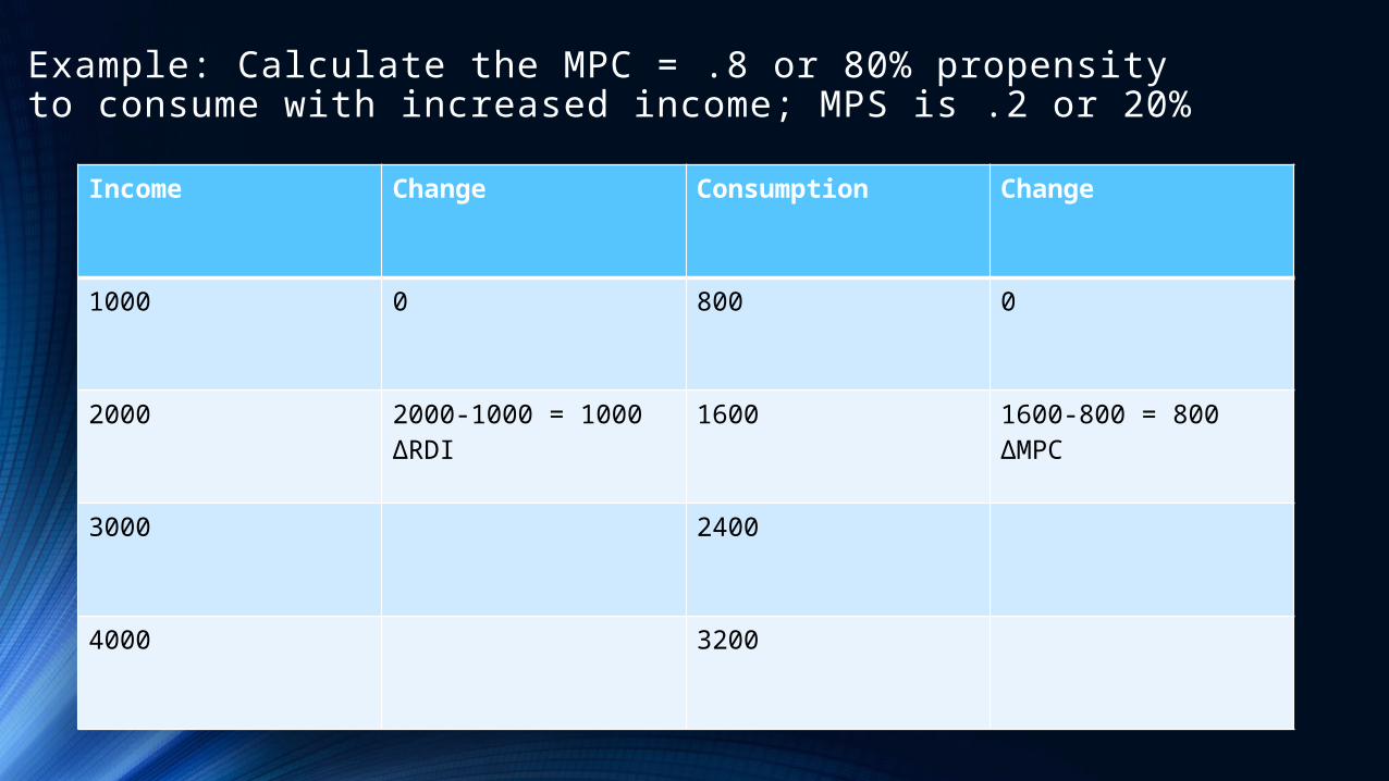
Example: Calculate the MPC = .8 or 80% propensity to consume with increased income; MPS is .2 or 20%

Income Change Consumption Change

1000 0 800 0

2000 2000-1000 = 1000∆RDI

1600 1600-800 = 800∆MPC

3000 2400

4000 3200

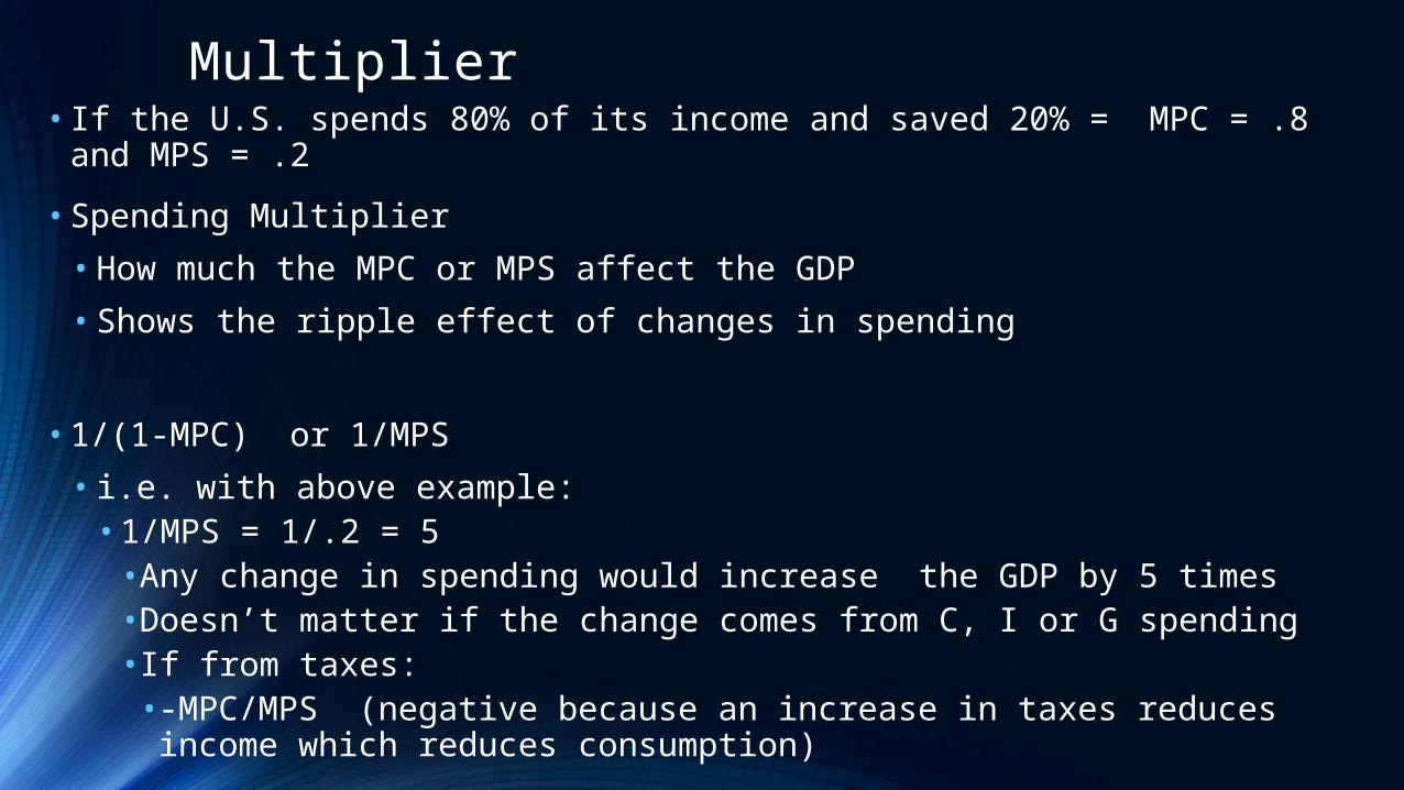
Multiplier• If the U.S. spends 80% of its income and saved 20% = MPC = .8 and MPS

= .2

• Spending Multiplier

• How much the MPC or MPS affect the GDP

• Shows the ripple effect of changes in spending

• 1/(1-MPC) or 1/MPS

• i.e. with above example:• 1/MPS = 1/.2 = 5• Any change in spending would increase the GDP by 5 times•Doesn’t matter if the change comes from C, I or G spending• If from taxes:• -MPC/MPS (negative because an increase in taxes reduces income which reduces consumption)

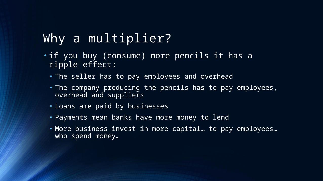
Why a multiplier?• if you buy (consume) more pencils it has a ripple effect:• The seller has to pay employees and overhead

• The company producing the pencils has to pay employees, overhead and suppliers

• Loans are paid by businesses

• Payments mean banks have more money to lend

• More business invest in more capital… to pay employees… who spend money…

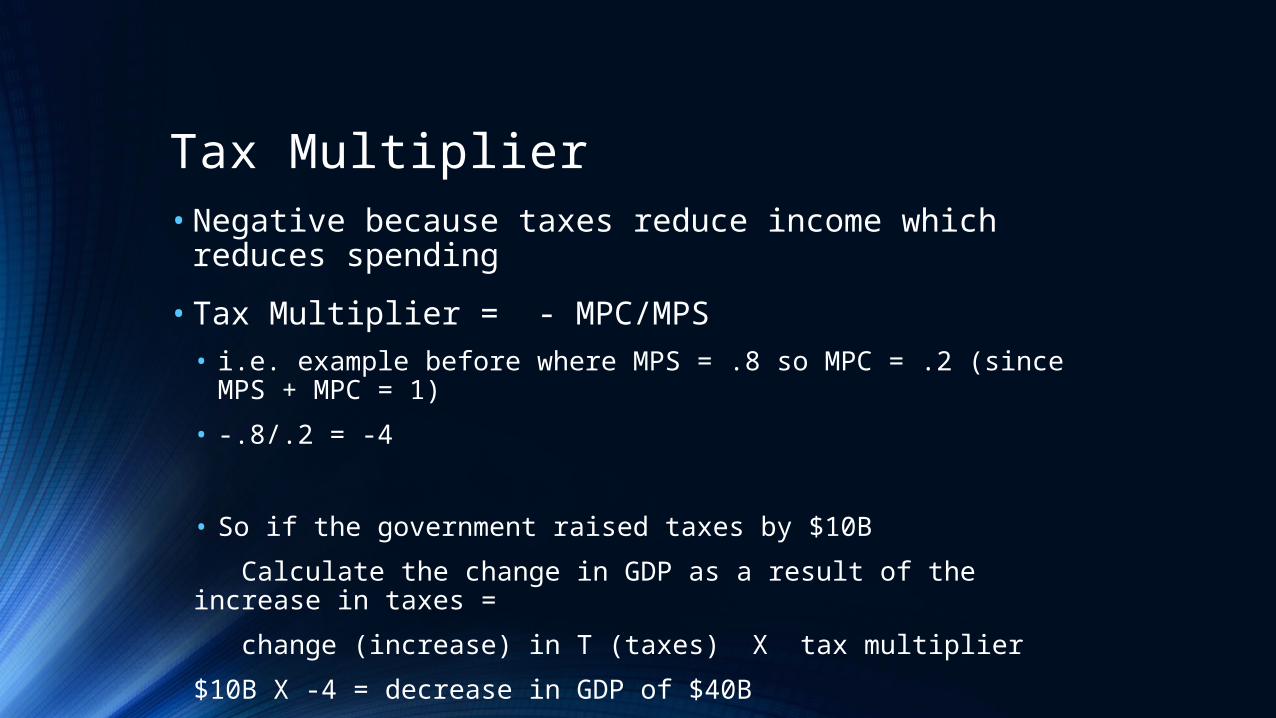
Tax Multiplier• Negative because taxes reduce income which reduces

spending

• Tax Multiplier = - MPC/MPS • i.e. example before where MPS = .8 so MPC = .2 (since MPS +

MPC = 1)

• -.8/.2 = -4

• So if the government raised taxes by $10B

Calculate the change in GDP as a result of the increase in taxes =

change (increase) in T (taxes) X tax multiplier

$10B X -4 = decrease in GDP of $40B

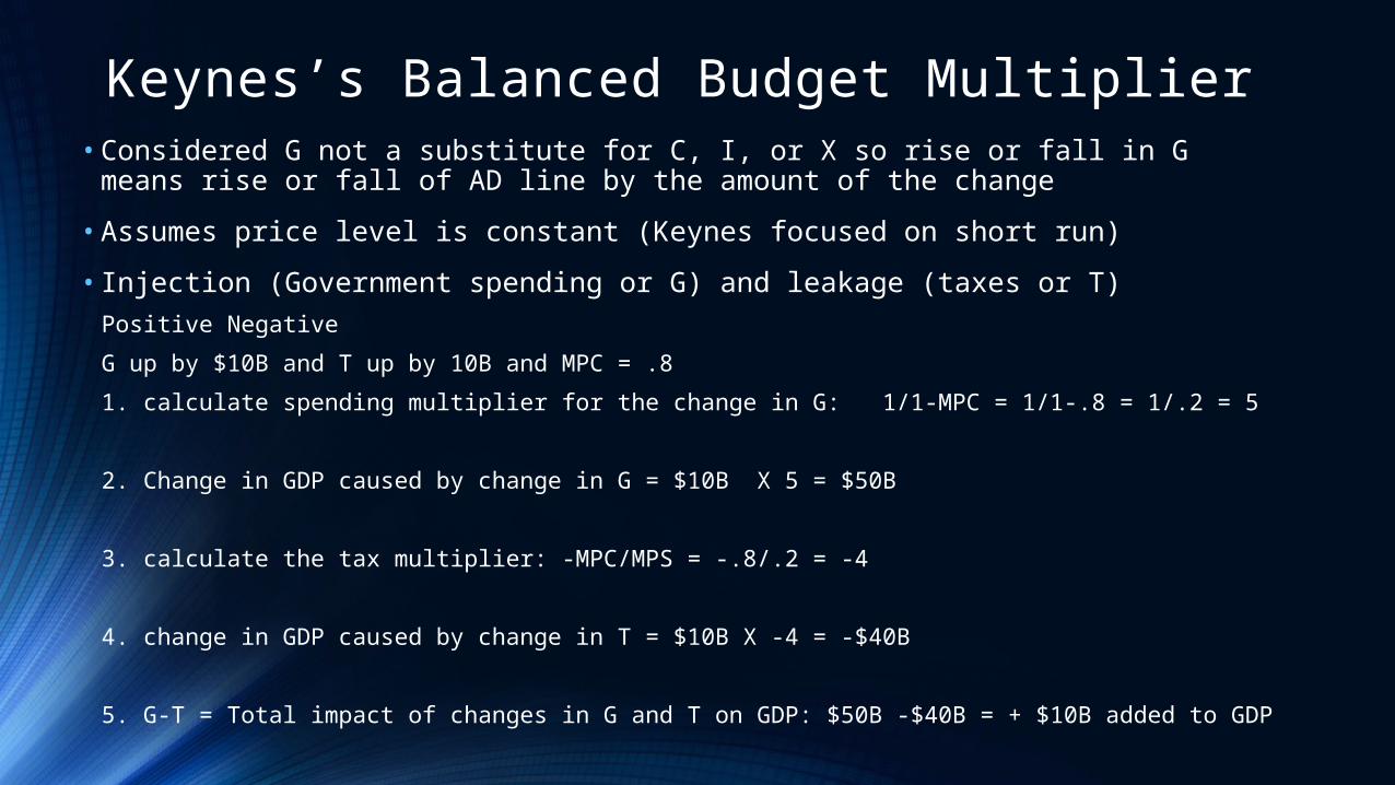
Keynes’s Balanced Budget Multiplier• Considered G not a substitute for C, I, or X so rise or fall in G means rise or fall

of AD line by the amount of the change

• Assumes price level is constant (Keynes focused on short run)

• Injection (Government spending or G) and leakage (taxes or T)Positive Negative

G up by $10B and T up by 10B and MPC = .8

1. calculate spending multiplier for the change in G: 1/1-MPC = 1/1-.8 = 1/.2 = 5

2. Change in GDP caused by change in G = $10B X 5 = $50B

3. calculate the tax multiplier: -MPC/MPS = -.8/.2 = -4

4. change in GDP caused by change in T = $10B X -4 = -$40B

5. G-T = Total impact of changes in G and T on GDP: $50B -$40B = + $10B added to GDP

Sample problem using Balanced Budget Multiplier• Government is spending up by $30B and taxes were raised by

$30B

• MPC = .7 MPS = .3

• 1/.3 = 3.3 = spending multiplier

• 3.3 X $30B = $99B

• -.7/.3 = - 2.3 = tax multiplier

• -2.3 X $30B = - $69B

• 99-69 = $30B difference to GDP

• Shift of AD upward

Shifts in Consumption Function• Any economic variable besides RDI

• i.e. Real Household Net Wealth (after debts are subtracted):

• Goes up, line shifts up

• Goes down, line shifts down

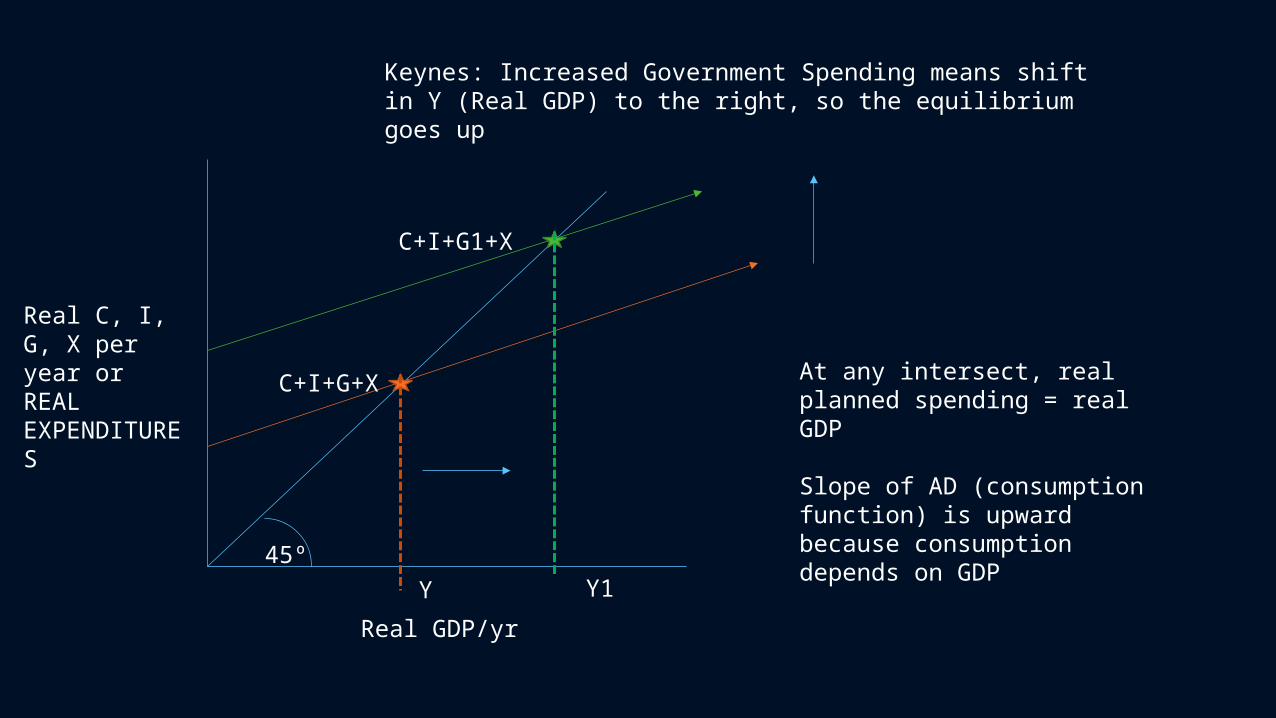
Keynes: Increased Government Spending means shift in Y (Real GDP) to the right, so the equilibrium goes up

45º

C+I+G1+X

C+I+G+X

Y Y1

Real C, I, G, X per year or REAL EXPENDITURES

Real GDP/yr

At any intersect, real planned spending = real GDP

Slope of AD (consumption function) is upward because consumption depends on GDP

Equilibrium

•Real Disposable Income = Real GDP – Real Net Taxes• (Real Net Taxes = Taxes – Transfer Payments)•Account for about 14- 21% of the GDP

Disposable Income (on average) = 82% of the GDP

Equilibrium Continued• Consumption as function of GDP

• Assumption that RDI differs from Real GDP by same amount each year

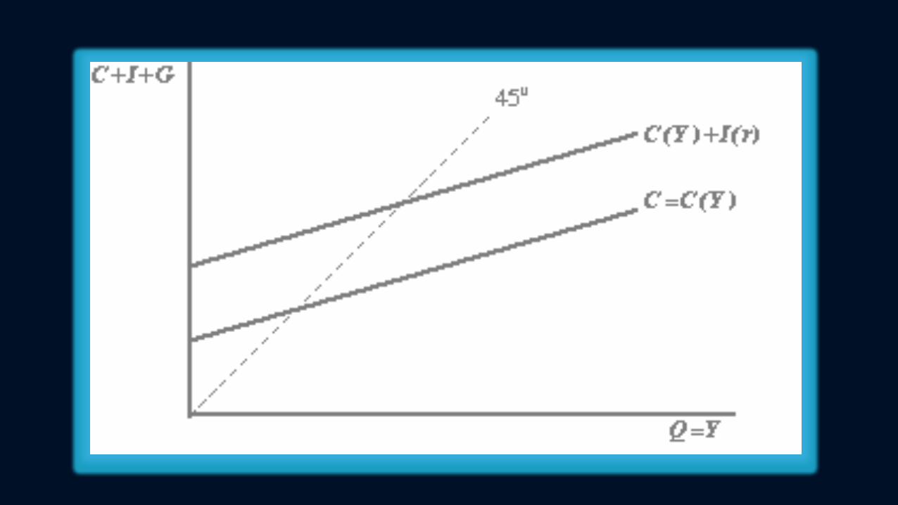
• Intersect with 45° is where real consumption expenditures equal real GDP• C = Y

• Investment Function

• I + C called consumption and investment line

• Intersect at 45° where expenditures (C + I) = real GDP • C + I = Y

The economy on a bigger scale• Investment:

• Flow

• Definition (in Economics): used to produce goods and services in the future; capital goods (fixed investment, non-consumable); inventory investment

• Planned Investment Function:• Only profitable if opportunity cost < return• Market interest rate determines amount of investment•Rate is down = planned investment up• Investment Function shows the inverse relationship between interest rate and value of planned real investment• Shifts: non-interest rate variables• i.e. business expenses, technology, taxes

Who cares?• The government uses GDP, CPI, and things like number of

building permits filed as LEADING INDICATORS for tracking the health of the economy.

• They use unemployment as well, but this is a LAGGING INDICATOR because of the long-term measurements (how long people are unemployed, how soon they find jobs and the figures change)

• COINCIDENTAL INDICATORS show things like how many employees are on payrolls or personal incomes

• Changes in these things are measured and applied to show trends. We can’t predict the future, but we can use the past as a guide (marginal changes over time)