Physics 247 Lab Manual Mechanics, Heat, Sound/Waves · S-2 Velocity of Sound in Air 50 ... Heading of the Experiment: Copy from the manual the number and name of the ... lab report

Physics 247 Lab Manual

Mechanics, Heat, Sound/Waves

R. Rollefson, H.T. Richards, M.J. Winokur, J.C. Reardon

September 13, 2016

Contents

Introduction 2

Errors and Uncertainties 4Characterization of Uncertainties . . . . . . . . . . . . . . . . . . . . . . . . 5Error Distribution and Error Bars . . . . . . . . . . . . . . . . . . . . . . . 6Propagation of Uncertainties . . . . . . . . . . . . . . . . . . . . . . . . . . 7Significant Figures . . . . . . . . . . . . . . . . . . . . . . . . . . . . . . . . 8

M-1 Errors & Motion 9M-1a Measurement and Error . . . . . . . . . . . . . . . . . . . . . . . . . 9M-1b Errors and the Density of a Solid . . . . . . . . . . . . . . . . . . . . 12M-1c Motion, Velocity and Acceleration . . . . . . . . . . . . . . . . . . . . 16

M-4 Acceleration in Free Fall 20

H-3 Latent heat of vaporization of liquid-N2 24

M-11b Air Track Collisions 27

M-7 Simple Pendulum 31

M-5 Projectile Motion 34

M-12b Simple Harmonic Motion and Resonance (Air Track) 37

S-1 Transverse Standing Waves on a String 46

S-2 Velocity of Sound in Air 50

A Appendices 51A Precision Measurement Devices . . . . . . . . . . . . . . . . . . . . . . . . . 51B PARALLAX and Notes on using a Telescope . . . . . . . . . . . . . . . . . 55

NOTE: M=Mechanics, H=Heat, S=Sound/Waves

1

INTRODUCTION 2

Introduction

General Instructions and Helpful Hints

Physics is an experimental science. In this laboratory, we hope you gain a realisticfeeling for the experimental origins, and limitations, of physical concepts; an awareness ofexperimental errors, of ways to minimize them and how to estimate the reliability of theresult in an experiment; and an appreciation of the need for keeping clear and accuraterecords of experimental investigations.

Physics is also a social activity. We expect you will find it useful to discuss all phases ofthe experiment with your lab partners. During set-up, establish the purpose of each pieceof apparatus; during data-taking, cooperate to choose who does what, and critique thedata as it is taken (is it as expected?); during analysis, perform calculations independently,and then compare results to check each others’ work; when drawing conclusions, debatethe reliability of the results, and what may fairly be concluded from them.

Maintaining a clearly written laboratory notebook is crucial. This lab notebook, at aminimum, should contain the following:

1. Heading of the Experiment: Copy from the manual the number and name of theexperiment.Include both the current date and the name(s) of your partner(s).

2. Original data: Original data must always be recorded directly into your notebookas they are gathered. “Original data” are the actual readings you have taken. Allpartners should record all data, so that in case of doubt, the partners’ lab notebookscan be compared to each other. Arrange data in tabular form when appropriate.A phrase or sentence introducing each table is essential for making sense out of thenotebook record after the passage of time.

3. Housekeeping deletions: You may think that a notebook combining all work wouldsoon become quite a mess and have a proliferation of erroneous and supersededmaterial. Indeed it might, but you can improve matters greatly with a little house-keeping work every hour or so. Just draw a box around any erroneous or unnecessarymaterial and hatch three or four parallel diagonal lines across this box. (This wayyou can come back and rescue the deleted calculations later if you should discoverthat the first idea was right after all. It occasionally happens.) Append a note tothe margin of box explaining to yourself what was wrong.

We expect you to keep up your notes as you go along. Don’t take your notebookhome to “write it up” – you probably have more important things to do than makinga beautiful notebook. (Instructors may permit occasional exceptions if they aresatisfied that you have a good enough reason.)

4. Remarks and sketches: When possible, make simple, diagrammatic sketches (ratherthan “pictorial” sketches” of apparatus. A phrase or sentence introducing eachcalculation is essential for making sense out of the notebook record after the passageof time. When a useful result occurs at any stage, describe it with at least a wordor phrase.

5. Graphs: There are three appropriate methods:

INTRODUCTION 3

A. Affix furnished graph paper in your notebook with transparent tape.

B. Affix a computer generated graph paper in your notebook with transparenttape.

C. Mark out and plot a simple graph directly in your notebook.

Show points as dots, circles, or crosses, i.e., ·, ◦, or ×. Instead of connecting pointsby straight lines, draw a smooth curve which may actually miss most of the pointsbut which shows the functional relationship between the plotted quantities. Fastendirectly into the notebook any original data in graphic form (such as the spark tapesof Experiment M4).

6. Units, coordinate labels: Whenever you write down a physical quantity, always writedown its units. Likewise, whenever you make a graph, always label the abscissa(horizontal coordinate) and ordinate (vertical coordinate), so that the reader (whomight be yourself at a later time) knows what has been graphed.

7. Final data, results and conclusions: At the end of an experiment some writtencomments and a neat summary of data and results will make your notebook moremeaningful to both you and your instructor. The conclusions must be faithful tothe data. It is often helpful to formulate conclusion using phrases such as “thediscrepancy between our measurements and the theoretical prediction was largerthan the uncertainty in our measurements.”

COMPLETION OF WORKPlan your work so that you can complete calculations, graphing and miscellaneous

discussions before you leave the laboratory. Your instructor will check each completedlab report and will usually write down some comments, suggestions or questions in yournotebook. Approach your instructor the way you would approach a senior colleague, whocan help deepen your understanding and “feel” for the subject.

ERRORS AND UNCERTAINTIES 4

Errors and Uncertainties

Reliability estimates of measurements greatly enhance their value. Thus, saying that theaverage diameter of a cylinder is 10.00±0.02 mm tells much more than the statement thatthe cylinder is a centimeter in diameter. The reliability of a single measurement (such asthe diameter of a cylinder) depends on many factors:

FIRST, are actual variations of the quantity being measured, e.g. the diameter ofa cylinder may actually be different in different places. You must then specify where themeasurement was made; or if one wants the diameter in order to calculate the volume,first find the average diameter by means of a number of measurements at carefully selectedplaces. Then the scatter of the measurements will give a first estimate of the reliability ofthe average diameter.

SECOND, the micrometer caliper used may itself be in error. The errors thus intro-duced will of course not lie equally on both sides of the true value so that averaging a largenumber of readings is no help. To eliminate (or at least reduce) such errors, we calibratethe measuring instrument: in the case of the micrometer caliper by taking the zero error(the reading when the jaws are closed) and the readings on selected precision gauges ofdimensions approximately equal to those of the cylinder to be measured. We call sucherrors systematic, and these cause errors in accuracy.

THIRD, Another type of systematic error can occur in the measurement of a cylin-der: The micrometer will always measure the largest diameter between its jaws; hence ifthere are small bumps or depressions on the cylinder, the average of a large number ofmeasurements will not give the true average diameter but a quantity somewhat larger.(This error can of course be reduced by making the jaws of the caliper smaller in crosssection.)

FINALLY, if one measures something of definite size with a calibrated instrument,one’s measurements will vary. For example, the reading of the micrometer caliper may varybecause one can’t close it with the same force every time. Also the observer’s estimate ofthe fraction of the smallest division varies from trial to trial. Hence the average of a numberof these measurements should be closer to the true value than any one measurement.


Characterization of Uncertainties

The experimenter cannot immediately determine the cause of the variation of a set ofmeasurements. A simpler task is to characterize this variation.

Consider the data below. Column 1 represents 10 readings of the diameter of a cylindertaken at one place, so that variations in the cylinder do not come into consideration. Themean of these 10 readings turns out to be 9.9427 mm. Column 2 gives the magnitude(absolute) of each reading’s deviation from the mean.

Measurements Deviation from Mean9.943 mm 0.00039.942 0.00079.944 0.00139.941 0.00179.943 0.00039.943 0.00039.945 0.00239.943 0.00039.941 0.00179.942 0.0007

How should one state the results of these measurements in a scientific fashion?A quick way to estimate the reliability of a set of measurements is to calculate the

average deviation from the mean. Expressed algebraically, the mean is x̄ =∑xi/n,

and the average deviation from the mean is = (∑|xi − x̄|)/n), where n is the number of

measurements taken and xi is the ith measurement.A more formal measure of the reliability of a set of measurements is the standard

deviation σ (also known as the “root mean square deviation”). You calculate σ as

σ =

√√√√ 1

(n− 1)

n∑i=1

(xi − x̄)2

Note that if you make one measurement of some quantity x, then n = 1 and x̄ = x1 in theabove equation: the standard deviation of your measurement is

√0/0, which is undefined.

You don’t know how reliable your measurement is.Assuming you make more than one measurement, σ tells you the typical deviation from

the mean you will find for an individual measurement. It depends on your experimentaltechnique. If you make more measurements, σ cannot be expected to change much.

However, the more measurements you make, the more accurately you can expect toknow the value of the mean. The uncertainty of the value of the mean is called thestandard deviation of the mean σµ, and in general it is less than σ:

σµ = standard deviation of the mean =σ√n

=1√n

√√√√ 1

n− 1

n∑i=1

(xi − x̄)2

The process of taking more measurements in order to minimize σµ is often referred to as“gathering statistics”.

One states one’s results as mean ± standard deviation of the mean. From thedata above, the diameter of the cylinder was measured to be 9.9427 ± 0.0004 mm.


Error Distribution and Error Bars

For a wide variety of measurements it may be assumed that the error distribution is“normal”: the probability of a given error ε is proportional to e−ε

2. If the error distribution

is normal, then on average 68% of a large number of measurements will lie closer than σto the true value.

The purpose of the error bars shown on a graph in a technical report is as follows: ifthe reader attempts to reproduce the results in the graph using the procedure describedin the report, the reader should expect his or her results to have a 50% chance of fallingwith the range indicated by the error bars.

If the error distribution is normal, the error bars should be of length ±0.6745σ.

For a clear discussion of the theory of errors, as it relates to experimental measurementsin the physical sciences, see P.R. Bevington and D.K Robinson, Data Reduction and ErrorAnalysis for the Physical Sciences, 3rd ed., McGraw Hill 2003, p. 11.


Propagation of Uncertainties

Let R = f(x, y, z) be a result R which depends on measurements of three different quan-tities x, y, and z. The uncertainty ∆R in R which results from an uncertainty ∆x in themeasurement of x is then

∆R =∂f

∂x∆x ,

and the fractional uncertainty in R is

∆R

R=

∂f∂x

f∆x .

In most experimental situations, the errors are uncorrelated and have a normal distribu-tion. In this case the uncertainties add in quadrature (the square root of the sum of thesquares):

∆R

R=

√√√√( ∂f∂x

f∆x

)2

+

(∂f∂y

f∆y

)2

+

(∂f∂z

f∆z

)2

.

Some examples:

A.) R = x + y. If errors in x and y each have a normal or Gaussian distributionand are independent, they combine in quadrature:

∆R =√

∆x2 + ∆y2 .

Note that if R = x− y, then ∆R/R can become very large if x is nearly equal to y. Henceavoid, if possible, designing an experiment where one measures two large quantities andtakes their difference to obtain the desired quantity.

B.) R = xy. If the measurement errors have a normal distribution and are independent,the relative errors combine in quadrature:

∆R

R=

√(∆x

x)2 + (

∆y

y)2 .

Note the same result occurs for R = x/y.C.) Consider the density of a solid (Exp. M1):

ρ =m

πr2L

where m = mass, r = radius, L = length, are the three measured quantities and ρ =density. Hence

∂ρ

∂m=

1

πr2L

∂ρ

∂r=−2m

πr3L

∂ρ

∂L=−mπr2L2

.

If the errors have normal distribution and are uncorrelated, then

∆ρ

ρ=

√(∆m

m

)2

+

(2

∆r

r

)2

+

(∆L

L

)2


Significant Figures

Suppose you have measured the diameter of a circular disc and wish to compute its areaA = πd2/4 = πr2. Let the average value of the diameter be 24.326± 0.003 mm; dividingd by 2 to get r we obtain 12.163± 0.0015 mm with a relative error ∆r

r of 0.001512 = 0.00012.

Squaring r (using a calculator) we have r2 = 147.938569, with a relative error 2∆r/r =0.00024, or an absolute error in r2 of 0.00024 × 147.93 · · · = 0.036 ≈ 0.04. Thus we canwrite r2 = 147.94 ± 0.04, any additional places in r2 being unreliable. Hence for thisexample the first five figures are called significant.

Now in computing the area A = πr2 how many digits of π must be used? A pocketcalculator with π = 3.141592654 gives

A = πr2 = π × (147.94± 0.04) = 464.77± 0.11 mm2

Note that ∆AA = 2∆r

r = 0.00024. Note also that the same answer results from π = 3.1416,but that π = 3.142 gives A = 464.83 ± 0.11 mm2 which differs from the correct value by0.06 mm2, an amount comparable to the estimated uncertainty.

A good rule is to use one more digit in constants than is available in your measure-ments, and to save one more digit in computations than the number of significant figuresin the data. When you use a calculator you usually get many more digits than you need.Therefore at the end, be sure to round off the final answer to display the correctnumber of significant figures.

SAMPLE QUESTIONS

1. How many significant figures are there in the following numbers?

(a) 976.45

(b) 4.000

(c) 10

2. Round off each of the following numbers to three significant figures.

(a) 4.455

(b) 4.6675

(c) 2.045

3. A function has the relationship Z(A,B) = A+B3 where A and B are found to haveuncertainties of ±∆A and ±∆B respectively. Find ∆Z in term of A, B and therespective uncertainties assuming the errors are uncorrelated.

4. What happens to σ, the standard deviation, as you make more and more measure-ments? what happens to σ, the standard deviation of the mean?

(a) They both remain same

(b) They both decrease

(c) σ increases and σ decreases

(d) σ approachs a constant and σ decreases

M-1 ERRORS & MOTION 9

M-1 Errors & Motion

M-1a Measurement and Error

OBJECTIVES:The major objectives of M-1a are to develop a basic understanding of what it meansto make an experimental measurement, and to provide a methodology for assessingrandom and systematic errors in this measurement process. In addition this lab willintroduce you to the PASCO interface hardware and software.

THEORY:How long is one second? The formal definition–the second is the duration of9,192,631,770 periods of the radiation corresponding to the transition between thetwo hyperfine levels of the ground state of the Cesium-133 atom–is unhelpful foreveryday affairs. In this lab you will test your ability to internalize the one secondtime interval by flicking your finger back and forth through an infrared beam sensoronce per second. The duration of each full cycle (back and forth, approximately2 seconds) will be simultaneously recorded, plotted and tabulated by the PASCOinterface software.

Your goal in this experiment is to learn to distinguish systematic and randomerrors, and assess the size of the systematic and random errors in your data set.SYSTEMATIC ERRORS: These are errors which affect the accuracy of a measure-ment. Typically they are reproducible so that they always affect the data in thesame way. For instance, if a clock runs slowly, its measurement of some durationwill be less than the true duration.RANDOM ERRORS: These are errors which affect the precision of a measurement.A process itself may have a random component (as in radioactive decay) or themeasurement technique may introduce noise that causes the readings to fluctuate.If many measurements are made, a statistical analysis will reduce the uncertaintyfrom random errors by averaging.

APPARATUS:

⇒ A PASCO photogate and stand: This device emits a narrow infrared beam in thegap and occluding the beam prevents it from reaching a photodetector. When thebeam is interrupted the red LED should become lit.

⇒ A PASCO 850 Universal Interface monitors the photogate output vs time and canbe configured to tabulate, plot and analyze this data.

PROCEDURE:

To configure the experiment you should refer to Fig. 1 below. Adjust the photogateso that one member can easily and repetitively flick his/her finger through the gap.Insert the phone-jack cable from the photogate into the DIGITAL INPUT #1 socket.

To launch the Pasco interface software, Capstone, you will need to click on the“Experiment M-1a” file in the PASCO/Physics201 folder on the desktop. Fig. 2below gives a good idea of how the display should appear.

You will note that a “dummy” first data set already exists on start-up showing atypical data run. In the table you can view all of the data points and the statisticalanalysis, including mean and standard deviation. In addition there should be a plotof this data and a histogram.


Figure 1: A schematic of the M-1a components and layout.

SUGGESTED PROCEDURE:

1. Start recording data by clicking on the “Record” icon and practice flicking afinger back and forth so that a two second interval appears in the window. The

Record icon has now changed to the “Stop” icon ; click the Stop icon when done.Since the program started with one set of data, this will produce a second set.

2. Each run gets its own data set in the “Data Summary” tab under the ToolsPalette. (If there are any data sets in existence you will not be able to reconfigurethe interface parameters or sensor inputs.) A data set can be deleted by selectingthe data set and clicking the red X to the right of the name. You can select whichdata set is displayed on a particular graph by clicking on the Data Summary iconthat appears on that graph.

Figure 2: The PASCO Capstone display window


3. Once you are comfortable with the procedure then click on the Record icon, cycle afinger back and forth over fifty times, then click on the Stop icon. DO NOT watchthe time display while you do this, since you want to find out how accurately andprecisely you can reproduce a time interval of 2 s using only your mind.

4. What is the mean time per cycle? What is the standard deviation? The mean t andstandard deviation σ are given by:

t =N∑i=1

ti/N and σ =

√√√√ N∑i=1

(ti − t)2/[N − 1] .

Click on the Statistics icon to ask PASCO to calculate the mean and standarddeviation of the data. Is your mean suggestive of a systematic error?

5. Look at the Histogram of the data. Does your data qualitatively give the appear-ance of a normal distribution (a Gaussian bell curve)?

6. For analyzing and quantifying random errors, you need to assess how a data set isdistributed about the mean. The standard deviation σ is one common calculationthat does this. In the case of a normal distribution approximately 68% of the datapoints fall within ±1σ of the mean (90% within ±2σ). Is your data consistent withthis attribute?

7. Assessing the possibility of systematic behavior is somewhat more subtle. In generalσ is a measure of how much a single measurement fluctuates from the mean. Inthis run you have made fifty presumed identical measurements. A better estimate ofhow well you have really determined the mean is to calculate the standard deviationof the mean σ = σ/

√N . After recording σ in your lab book, can you now observe

any evidence that there is a systemic error in your data? Answer this same questionwith respect to the first “sample” data set.

8. OPTIONAL: Systematic errors can sometimes drift over time. In the best-casescenario they drift up and down so that they average out to zero. (Clearly it wouldbe better if they could be eliminated entirely.) With respect to t and σ for the first25 and second 25 cycles do you observe any systematic trends? Click on the Data

Highlight icon . Dragging the mouse will highlight a subset of the data. Themean, σ, and other statistical attributes will appear at the bottom of the table.


M-1b Errors and the Density of a Solid

OBJECTIVES:

To learn about systematic and random errors; to understand significant figures; toestimate the reliability of one’s measurements; to propagate uncertainties; and tocalculate the reliability of the final result.

NOTE: This experiment illustrates the earlier section on Errors and Uncertainties.The accuracy of your estimate of reliability will show whether you have masteredthe material in this section.

APPARATUS:

Metal cylinders of varying sizes; micrometer; vernier calipers; precision gaugeblocks; precision balance.

PRECAUTIONS:

Avoid dropping the metal cylinders, or deforming them in any other way.

Avoid damage to the precision screw of the micrometer by turning only the ratchetknob to open or close the jaws.

The caliper has a lock which lets you preserve a reading—be sure to disengage thecaliper lock before using.

Improper weighing procedures may damage the precision balance. Consult yourinstructor if in doubt.

In handling the gauge blocks avoid touching the polished surfaces since body acidsare corrosive.

INTRODUCTION:

First read the material on Errors and Uncertainties and Significant Figures in thelab manual Introduction. Since density is the mass per unit volume, you mustmeasure the mass (on a balance), and compute the volume (hπr2 = hπd2/4) frommeasurements of the cylinder’s diameter d and height h. Any one of three length-measuring devices may be used. These include a micrometer, a vernier caliperand/or a simple metric ruler. The micrometer will permit the highest precisionmeasurements but using one can be cumbersome, especially when reading the vernierscale. All methods will demonstrate the aforementioned objectives. Your instructorwill give you guidance in choosing an appropriate measurement device.

THE MICROMETER:

Record the serial number of your micrometer. Then familiarize yourself with theoperation of the caliper and the reading of the scales: work through Appendix Aon the Micrometer. Note that use of the ratchet knob in closing the jaws insuresthe same pressure on the measured object each time. Always estimate tenths of thesmallest division. Some micrometers have verniers to assist the estimation.


THE VERNIER CALIPER:

The vernier scale was invented in 1631 by Pierre Vernier. Work through AppendixA for practice reading a vernier scale. Experiment with one of the large verniers inthe lab until you are confident you can use it correctly.

Precautions on use of the calipers:

1. Unclamp both top thumbscrews to permit moving caliper jaws.

2. Open caliper to within a few mm of the dimension being measured.

3. Close right thumbscrew to lock position of lower horizontal knurled cylinder, whichexecutes fine motions of caliper jaw. Never over tighten!

CALIBRATION:

1. Zero Error: For those using the calipers: wipe the caliper jaws with cleaningpaper. Close the jaws and make a reading. Record the reading, separate the jaws,close them again, and make another reading. Continue in this way until you haverecorded five readings. The mean of these readings is the zero error. The variationof the readings gives you an estimate of the reproducibility of caliper measurements.

For those using the micrometers: follow the same procedure above; refer to AppendixA for instruction on how to read the zero error.

2. Measure all four calibration gauge blocks (6, 12, 18 and 24 mm): Set the gaugeblocks on end, well-in from the edge of the table, and thus freeing both hands tohandle the caliper. Record the actual (uncorrected) reading. A single measurementof each block will suffice.

3. Plot a correction curve for your measuring device: plot errors as ordinates andnominal blocks sizes (0, 6, 12, 18, and 24 mm) as abscissa. Normally the correctionwill not vary from block to block by more than 0.003 mm (for the micrometer). Ifit is larger, consult your instructor.

DENSITY DETERMINATION:

1. Make five measurements (should be in millimeters) of the height and five of thediameter. Since our object is to determine the volume of the cylinder, distributeyour measurements so as to get an appropriate average length and average diameter.Avoid any small projections which would result in a misleading measurement. If notpossible to avoid, estimate their importance to the result. Record actual readingsand indicate, in your lab book, how you distributed them.

2. Calculate the average length, average diameters and the respective standard devia-tion.

3. Use your correction curve to correct these average readings. If you were to use theuncorrected values, how much relative error would this introduce?

4. Weigh the cylinder twice on the electronic balance; estimate to 0.1 mg.


5. From the average dimensions and the mass, calculate the volume and density. Makea quantitative (refer to the Propagation of Uncertainties section on page 7) estimateof the uncertainty in the density. The sample worksheet asks for both the maximumand minimum values. You should use, as your starting point:

Density(ρ±∆ρ) = ρ(h±∆h, d±∆d,m±∆m) =m

π(d/2)2 h

6. Compare the density with the tabulated value. Tabulated values are averages oversamples whose densities vary slightly depending upon how the material was cast andworked; also on impurity concentrations.

7. Summarize the data and results in your notebook. Also record your result on theblackboard. Is the distribution of blackboard values reasonable, i.e. is it a “normal”distribution (refer to the section on page 6)?

To test how accurately you can estimate a fraction of a division, estimate the frac-tions on the vernier caliper before reading the vernier. Record both your estimateand the vernier reading.

Link to the world’s premier institution devoted to improving the accuracy of mea-surements:

National Institute of Science & Technology at http://www.nist.gov/


Experiment 1b Worksheet

1.CALIBRATION TABLE

Micrometer Serial # =MEASUREMENTS

Zero gap 1 = ±2 =3 =4 =5 =

Mean±σ= ±Gauge block 6 mm

12 mm18 mm24 mm

2. Make a plot of Gauge block thickness (x-axis) versus Micrometer reading.Next fit the data to a line; this generates a correction curve whereCorrected value = actual × slope + interceptslope =intercept =

3. Now for the unknown value:

CYLINDER Height (± ) Width (± ) Mass (± )1=2=3=4=5=

Mean±σ = ± ± ±Corrected Mean±σ= ± ± ±

Density =Max. Density =Min. Density =

4. Final result, density = ±

5. Cut and tape this into your lab notebook.

6. Answer the following questions in your notebook.A. Identify two sources of systematic error and give their magnitude.B. Identify two examples of random error and give their magnitude.


M-1c Motion, Velocity and Acceleration

OBJECTIVES:

The two objectives of this exploratory computer lab are: become familiar withthe PASCO interface hardware and software; develop an intuition for Newtonianmechanics by experimenting with 1-D motion.

THEORY:

The motion of an object is described by indicating its distances x1 and x2 from afixed reference point at two different times t1 and t2. From the change in positionbetween these two times one calculates the average velocity (remember velocity is avector, and specifies direction) for the time interval:

average velocity ≡ v =x2 − x1

t2 − t1=

∆x

∆tm/s

The acceleration of an object may be calculated by finding its velocity v1 and v2 attwo different times t1 and t2. From the change in velocity between t1 and t2 onecalculates the average acceleration for the time interval:

average acceleration ≡ a =v2 − v1

t2 − t1=

∆v

∆tm/s2

FUNDAMENTAL CONCEPTS OF LINEAR MOTION:

1. The equation that describes the motion of an object that moves with constant ve-locity is: x = A+B · t.If you make a plot of x versus t, you find that it describes a straight line. The letterA indicates the position of the object at time t = 0. The letter B is the slope of theline, and is equal to the velocity of the object. So we can rewrite this x = x0 + v · t.

2. The equation that describes the motion of an object that moves with constant ac-celeration is: x = x0 + v0 · t+ 1

2at2 and v = v0 + at.

So we can rewrite this as: x = A + Bt + Ct2 and v = B + 2Ct. A indicates theposition of the object at time t = 0. B is the the velocity of the object at time t = 0,and is the slope of the graph at this time. C is equal to half the acceleration.

PRECAUTIONS:

In order for the motion sensor to work properly it must be pointed in such awaythat it “sees” the vane, and doesn’t “see” the front of the cart; that means thatit must be pointed slightly upwards. The motion sensor tends to “see” the closestreflecting surface. In addition the minimum range is approximately 20 cm.

Make sure you do not drop the carts or allow them to roll off the table.This damages the bearings and drastically increases the friction.


APPARATUS

⇒ A PASCO motion sensor; this device emits a series of short pulses of sound, andreceives a series of echoes reflected from a nearby object. The length of the timeinterval between the emission and the reception of the sound pulse depends on thedistance to the reflecting object.This method of locating an object is the same as the one used by bats to find flyinginsects or by navy ships to locate submarines.

⇒ A PASCO Interface; this converts the time interval between the emission and re-ception of the sound pulse to digital form, i.e., numbers that can be stored by thecomputer. Connect yellow plug to digital channel 1.

⇒ PASCO dynamic track with magnetic bumpers; cart with reflecting vane; meterstick; one or two steel blocks.

PROCEDURE:

Your instructor will demonstrate how to configure the experiment. To initiate thePASCO interface software you will need to double click the “Experiment M-1c” filein the PASCO/Physics201 folder on the desktop. Fig. 1 below shows how the displayshould appear. All three measured quantities, position, velocity, and acceleration,are displayed simultaneously. Since velocity is determined from the position dataand acceleration from the velocity the “scatter” in the data will become progressivelymore pronounced.

Figure 1: The PASCO Capstone display format

EXPERIMENT I: BASIC OPERATION AND MOTION SENSOR CALIBRATION:

1. To start the data acquisition click on the Record icon . To stop it click on the

same icon which will now become the Stop icon . Each run gets its own data set

in the Data Summary tab under the Tools Palette. If there are any data sets


in existence you will not be able to reconfigure the interface parameters or sensorinputs, unless you clear (delete) all data.

2. With the data acquisition started move the cart to and fro and watch the position,velocity and acceleration displays.

3. Stop the data acquisition.

4. Click on the Zoom-to-Fit icon on one of the plots. Click on the Data Highlight

icon and the Zoom-to-Fit icon to zoom in to particular regions of interest.

Use Ctrl-Z to get back to the original plot area. Click on the Crosshair icon

and move about within a plot window. Click on the Statistics icon to bring upstatistics for a given set of data. Make sure that all members of the group have anopportunity to test these components. It will facilitate the rest of the course if thebasic operations on the software interface are understood by everyone!

5. Delete the data set by clicking on the red ‘X’ next to RUN #1 item in the Data

Summary tab under the Tools Palette.

6. Start the data acquisition and find the closest distance to the motion sensor at whichit still functions. This value is supposed to be close to 20 cm. If it is much larger,re-aim the motion sensor.

7. Configure the distances so that when the cart nearly touches the near magneticbumper the motion sensor still records accurately.

8. Measure the position at two distances approximately 0.8 m apart and compare theprinted centimeter scale with the motion sensor readout. By how much do thereadings differ?

EXPERIMENT II: INCLINED PLANE AND MOTION:

1. Raise the side of the track closest to the position sensor using one of the suppliedblocks.

2. Find an appropriate release point that allows the cart to roll down the track slowlyenough that it bounces off the magnetic bumper without striking it.

3. Click the Record button and release the cart, letting it bounce three or four times,and then click the Stop button.

4. Qualitatively describe the shape of the three curves: position, velocity and acceler-ation and discuss how they evolve with time.

5. Obtain a hard copy of this data by pressing CTRL-p.

6. Label/identify the various key features in the various curves by writing directly onthe hard copies. Paste the graphs in your note book.

QUESTIONS: (to be discussed as a group)

1. Does the velocity increase or decrease linearly with time when the cart is slidingup/down the track?


2. When the velocity is close to zero can you observe any nonlinear oscillations in thedata? Can you think of a reason for any deviations from linearity?

3. Why does the cart bounce less high with each subsequent bounce?

4. Is the collision with the magnetic bumper or the residual friction in the bearing themost likely source of loss?

5. Can you think of a method using your data to determine which of these two proposedmechanisms is the most likely culprit?

EXPERIMENT III: MOVING THE CART BY HAND:

1. Remove the block so that the track is no longer raised.

2. Start a new data set (by clicking the Record button) and try to move the cart backand forth at constant velocity using your hand from the side.

3. Using the cross hair estimate the velocity in either m/s or cm/s.

4. Repeat step 2, but now try to obtain (for a limited time) a constant acceleration.

EXPERIMENT IV: ACCELERATION AT g (9.8 m/s2):

1. Have one member of the group stand carefully on a chair and hold the position sensorfacing downward above a second member’s head, while the second member holds anotebook above his or her head.

2. Start a new data set and have the student holding the notebook jump up and downa few times.

3. Stop the recording and determine whether free-fall yields a constant accelerationclose to the accepted value.

4. Try to measure the acceleration by making fits to data. First use the Data Highlight

icon to choose a range of data. Then click on the Fit icon to get at thepull-down menu. You have three choices: fit a quadratic function to the positiondata, fit a straight line to the velocity data, or find the mean of the acceleration.Which method seems least accurate? Which seems most accurate?

M-4 ACCELERATION IN FREE FALL 20

M-4 Acceleration in Free Fall

OBJECTIVE: To measure g, the acceleration of gravity; to propagate uncertainties.

APPARATUS:

Free fall equipment: cylindrical bobs (identical except in mass) which attach to papertape for recording spark positions; spark timer giving sparks every 1/60 second;cushion; non-streamline bobs to study air resistance (by adding a front plate).

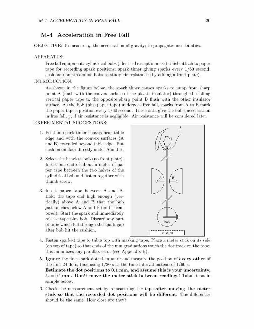
INTRODUCTION:

As shown in the figure below, the spark timer causes sparks to jump from sharppoint A (flush with the convex surface of the plastic insulator) through the fallingvertical paper tape to the opposite sharp point B flush with the other insulatorsurface. As the bob (plus paper tape) undergoes free fall, sparks from A to B markthe paper tape’s position every 1/60 second. These data give the bob’s accelerationin free fall, g, if air resistance is negligible. Air resistance will be considered later.

EXPERIMENTAL SUGGESTIONS:

1. Position spark timer chassis near tableedge and with the convex surfaces (Aand B) extended beyond table edge. Putcushion on floor directly under A and B.

2. Select the heaviest bob (no front plate).Insert one end of about a meter of pa-per tape between the two halves of thecylindrical bob and fasten together withthumb screw.

3. Insert paper tape between A and B.Hold the tape end high enough (ver-tically) above A and B that the bobjust touches below A and B (and is cen-tered). Start the spark and immediatelyrelease tape plus bob. Discard any partof tape which fell through the spark gapafter bob hit the cushion.

A B

bob

cushion

4. Fasten sparked tape to table top with masking tape. Place a meter stick on its side(on top of tape) so that ends of the mm graduations touch the dot track on the tape;this minimizes any parallax error (see Appendix B).

5. Ignore the first spark dot; then mark and measure the position of every other ofthe first 24 dots, thus using 1/30 s as the time interval instead of 1/60 s.Estimate the dot positions to 0.1 mm, and assume this is your uncertainty,δr = 0.1 mm. Don’t move the meter stick between readings! Tabulate as insample below.

6. Check the measurement set by remeasuring the tape after moving the meterstick so that the recorded dot positions will be different. The differencesshould be the same. How close are they?


EXAMPLE OF TABULAR FORM FOR DATA:

Dot Time Position Average velocity Average accelerationi t(i) r(i) v(i) a(i)

sec cm cm/sec cm/sec2

δt = δr = δv = δa =

0 t(0) a — —1 t(1) b b− a (c− b)− (b− a)2 t(2) c c− b (d− c)− (c− b)3 t(3) d d− c (e− d)− (d− c)4 t(4) e e− d (f − e)− (e− d)5 t(5) f f − e (g − f)− (f − e)6 t(6) g g − f (h− g)− (g − f)7 t(7) h h− g (i− h)− (h− g)8 t(8) i i− h (j − i)− (i− h)9 t(9) j j − i (k − j)− (j − i)

10 t(10) k k − j (l − k)− (k − j)11 t(11) l l − k (m− l)− (l − k)...

......

......

SUGGESTIONS ON HANDLING DATA:

1. Analysis may be conveniently done using Excel.

2. Record your estimates of the uncertainties in measurement: δt, the uncertainty inthe times of the sparks; δr, the uncertainty in the positions of the dots on the paper.

3. Let t = 0 represent where your readings start (the actual starting value is arbitrary).Tabulate the readings, r(i), on the meter stick at the end of each time interval as incolumn 3 above.

4. Calculate the average velocity, v in each interval; then calculate the average accel-eration, a during each interval, as shown in the table.

5. Calculate the uncertainty in each measurement of v and a by using the appropriatetechnique described in “Propagation of Uncertainties” on page 7, and record it inyour table.

6. Define 〈a〉 to be the average of all the readings in the “average acceleration” column.Find 〈a〉. This “average of the average” is more accurate than fluctuations in thea column might indicate. Explain why. (Hint: Are the values independent? Seesuggestion 8, below.)

7. With 1/30 s as the time interval, plot r vs time, v vs time, and a vs time. Notethat for v the value is the average of v between to adjacent rows, i and i + 1, andtherefore equals the instantaneous v at the middle of the interval.

8. Plot velocity as a function of time. Fit a straight line to the plot; equate the slopeof the fit to the acceleration, and the uncertainty in the slope to the uncertainty inthe acceleration. This approach is a better way of using all the data than the abovenumerical one since averaging the a column involves summing the a column and insuch a sum all readings except (b− a) and (m− l) drop out!


ERROR ANALYSIS:

Spark timing errors are negligible. However, spark position errors are not. The sparkin the spark timer does not follow the same path every time. Assume the deviation ofthe path of a particular spark from the mean spark path is characterized by σ = 0.5mm. Thus the computed value of (b − a) would be subject to an error ∼ 0.7 mm.This is in excess of the 0.1 mm measurement uncertainty.

However, successive measurements of v are correlated: since v(1) ∝ b−a and v(2) ∝c − b, a fluctuation in b will always push v(1) and v(2) apart. This in turn meansthe uncertainty calculated for the slope of v̄ will be larger than it really is.

Calculate the slope using only every other v(i) because v(1), v(3), v(5) etc. use in-dependent data. Estimate the uncertainty in the slope. Compare to the uncertaintyin the slope calculated in step 8 above.

Calculate g, the free-fall acceleration of the bob, using whichever method gives thesmallest uncertainty, and record both g and the uncertainty.

QUESTION:

The local value of g has been measured to be 9.803636 ± 0.000001 m/s2.1 Is thediscrepancy between this value of g and your value of g larger or smaller than theuncertainty in your value of g?

OPTIONAL EXPERIMENTS

A. EQUIVALENCE OF GRAVITATIONAL AND INERTIAL MASS:

Galileo showed (crudely) that the acceleration of falling bodies was independent ofthe mass. Check Galileo’s experiment by measuring the free-fall acceleration of thelight plastic bob (identical in size and shape to the heavy metal bob), and comparingit to the free-fall acceleration of the heavy metal bob.

Is the difference between the two measurements of the free-fall acceleration largerthan the uncertainties in both, or smaller than the uncertainty in either, or some-where in between?

B. EFFECT OF AIR RESISTANCE:

The effect of air resistance is small for streamlined objects at low velocities, but canbecome large for non-streamlined objects, such as a parachute. To quantify it, firstmake both bobs non-streamlined by inserting into the bottom of the bob the bananaplug holding a small flat plate. Then repeat the experiment for the non-streamlinedbobs. Since the force of air resistance, f(v), is a function of only velocity if thesize, shape and roughness are the same, then f(v) on the two bobs will be almostthe same since their velocities are similar. The net force on the falling body is thenF = mg − f(v). Hence

a =F

m=mg − f(v)

m= g − f(v)

m

1Wollard and Rose, “International Gravity Measurements”, UW Geophysical and Polar Research Cen-ter, (1963) p. 211 and p. 236.


and

〈a〉 ≈ g −(

1

m

)〈f(v)〉 .

Thus if we measure 〈a〉 for bobs identical except in mass and plot 〈a〉 against 1/m,we should obtain a straight line. The slope of this line is the force 〈f(v)〉 due to airresistance, and the extrapolation of the line to (1/m) = 0 gives g.To improve the accuracy of your measurements of 〈f(v)〉 and g, pool your datawith other lab groups.

C. MEASUREMENT OF REACTION TIME BY FREE FALL:

(1) Have your partner hold the vertical meter stick while you place your thumb andforefinger opposite the 50 cm mark but not grasping it. When your partnerreleases the stick, grab it as soon as possible. From the distance through whichthe 50 cm mark fell, calculate the time of free fall of the meter stick. This isyour “reaction time”.

(2) With thumb and forefinger, grasp a vertical meter stick at the 50 cm mark.Release and grab it again as quickly as possible. From the distance throughwhich the 50 cm mark fell, calculate the time of free fall of the meter stick.This is your “time scale for coordinated movement”. Compare this time toyour reaction time. Why might the two be different?

OPTIONAL QUESTIONS:

1. Estimate the effect on your value of g of the air’s buoyant force, Fa. For air density,use ρ = 1.2 kg/m3 and for brass density (bob), ρbob = 8700 kg/m3.

Hints: Fa = ρambobg/ρbob (why?); a = g[1− (ρa/ρbob)] (why?)

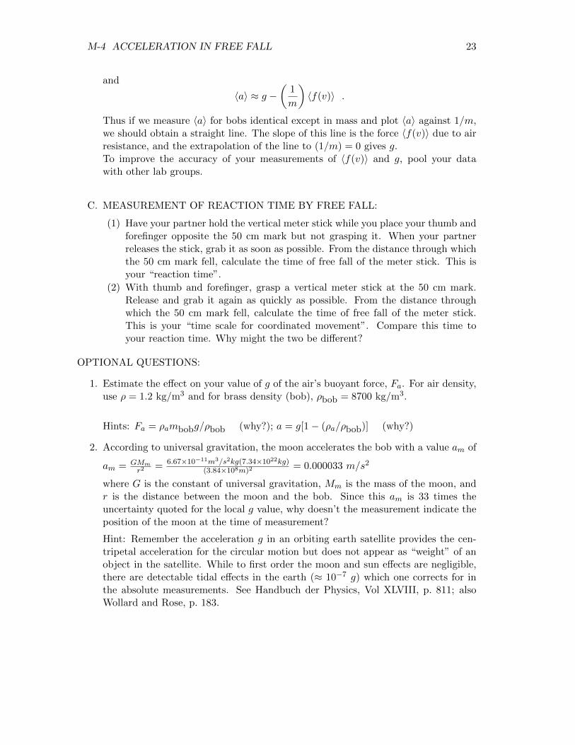
2. According to universal gravitation, the moon accelerates the bob with a value am of

am = GMmr2

= 6.67×10−11m3/s2kg(7.34×1022kg)(3.84×108m)2

= 0.000033 m/s2

where G is the constant of universal gravitation, Mm is the mass of the moon, andr is the distance between the moon and the bob. Since this am is 33 times theuncertainty quoted for the local g value, why doesn’t the measurement indicate theposition of the moon at the time of measurement?

Hint: Remember the acceleration g in an orbiting earth satellite provides the cen-tripetal acceleration for the circular motion but does not appear as “weight” of anobject in the satellite. While to first order the moon and sun effects are negligible,there are detectable tidal effects in the earth (≈ 10−7 g) which one corrects for inthe absolute measurements. See Handbuch der Physics, Vol XLVIII, p. 811; alsoWollard and Rose, p. 183.

H-3 LATENT HEAT OF VAPORIZATION OF LIQUID-N2 24

H-3 Latent heat of vaporization of liquid-N2

OBJECTIVE:

To measure the heat of vaporization of liquid nitrogen, Lv, at its boiling point(Tb = 77 K at standard atmospheric pressure).

APPARATUS:

Dewar flask; liquid nitrogen (ask for help in getting it from a large storage De-war in room 4329 Chamberlin Hall); aluminum cylinder on a long thread; doublepan balance; calorimeter plus water jacket for thermal ballast (as in H-2a); timer;thermocouple-type digital thermometer; selection of slotted masses; coffee pot forhot water.

PRECAUTIONS:

Liquid N2 is fascinating to work with. However, keep in mind the following simplesafety precautions.

1. Never stopper a flask of liquid N2 with an unperforated stopper. Thiscan result in a dangerous explosion with risk of major injury. Stu-dents found attempting this will be referred to the Dean of Studentsfor disciplinary action.

2. Have a perforated stopper on the Dewar throughout the experiment to preventcondensation of moisture from the air on the inside of the flask.

3. Avoid prolonged contact of liquid N2 with your skin. The insulatingvapor layer may disappear and severe frost-bite may result.

INTRODUCTION:

When one lowers an aluminum cylinder of mass mAl, that is at room temperature,Tr, into liquid N2 at its boiling temperature, Tb, the cylinder cools to Tb. The heatgiven off during this cooling, QAl, will vaporize a mass mN of liquid N2.

You might expect to find Lv, of the nitrogen by setting

mNLv = QAl = mAlcAl(Tr − Tb) .

This method fails because cAl is not constant over the ∼ 220◦C temperature rangebetween Tr and Tb. See figure 1.

We can avoid this difficulty by noting that QAl is also the heat needed to warm thesame aluminum cylinder to from Tb to Tr. You can measure this heat by placing thecold aluminum cylinder (at temperature Tb) in a “calorimeter” that contains waterand observing the change in temperature of the water, −∆T , –provided that thefinal temperature of the water, Tf , is room temperature, Tr. It is hard to arrangefor Tf to end up exactly at room temperature, but if Tf is close to Tr, one canaccurately correct the calorimeter data for the small additional heat term, namelymAlcAl(Tr − Tf ), since over the small Tr − Tf interval, cAl = 0.212 cal/g/K isconstant.

SUGGESTIONS ON PROCEDURE:

1. To maximize sensitivity (i.e. to get a large temperature change in the water) useonly enough water (∼125-150 grams) in the calorimeter to cover the metal cylinder.


-300 -200 -100 0 100T (˚C)

CAl

.1

.2

kca

l/kg

Tb

Tr

Figure 1: Specific heat capacity of Al vs. temperature.

2. The calorimeter is designed to thermally isolate the water from the surroundings.The inner vessel of the calorimeter is mounted within, but thermally isolated from,a surrounding water jacket, which is close to room temperature. The isolation isn’tperfect, so here will be some small amount of heat flow between the calorimeter andthe jacket. To minimize the net heat exchange with the water jacket, you will wantto make the initial water temperature as far above the jacket temperature as youexpect it to end up below the jacket temperature after the water in the inner vesselhas been cooled by your Al cylinder. (The jacket temperature will remain fairlyconstant during the experiment.) Estimate roughly the proper initial water andcalorimeter temperature. [Use the measured mass of the aluminum cylinder, mAl,its specific heat (0.212 kcal/kg◦C) and the b.p. of liquid N2, Tb = 77 K. For thisrough calculation, assume that the specific heat of Al is constant with temperature.]Determine the water mass, mw, and appropriate starting temperature.

3. Place the flask containing liquid nitrogen (plus perforated stopper) on one pan ofa balance and record the mass each minute for 10 minutes. (Why is the massdecreasing?)

4. Record the temperature of the metal cylinder, TR, and then lower it (by a thread)gently to the bottom of the flask. Replace the stopper (perforated) on the top ofthe flask and continue recording the total mass each minute until it shows a slowsteady decrease.

5. Record the initial temperature, Ti, of the calorimeter, which you have chosen socleverly in section 2. Transfer the cold metal cylinder into the calorimeter, andnote the calorimeter temperature every two minutes (while gently stirring). Recordthe mass of the flask of liquid N2 on alternate minutes. When the calorimetertemperature has reached a slow steady rate of change and the mass of the flask ofliquid N2 is falling at a slow steady rate, discontinue the readings.


6. Plot the mass of the flask plus nitrogen as a function of time. For the minutes thatthe cylinder of metal was in the flask, subtract the mass of the cylinder. See thefigure for a typical plot.

t

m

ab

cd

e

f

g

How much of the N2 mass changewas caused by the heat from thecylinder? If a-b and c-d were paral-lel, it would be the vertical distancebetween these lines. But c-d ordi-narily has a smaller slope than a-b,possibly because the evaporation ofliquid nitrogen between b and c hascooled the upper part of the flask.

Hence we use the average of the two rates of fall by drawing a vertical line throughe, (the midpoint of line b-c). Then f-g estimates the mass, mN , evaporated by theheat from the cylinder.

7. The final temperature, Tf , of the Al cylinder in the calorimeter usually will notbe quite the same as the initial temperature (= Tr) of the cylinder before it waslowered into the liquid nitrogen.

Hence QAl will be the heat to warm the Al cylinder in the calorimeter to Tf plusthe mass of the cylinder × (specific heat of aluminum) × (Tr − Tf ).

Specifically if:

Lv = latent heat of vaporization of nitrogenmN = mass of nitrogen evaporated by heat from the cylindermAl, cAl= mass and specific heat of Al cylinder

Ti = initial temperature of water and calorimetermw, cw = mass and specific heat of watermc, cc = mass and specific heat of calorimeter and stirrer

ht = heat capacity of immersed part of thermometer,

then, if we neglect ht:

QAl = mNLv = (mwcw + mccc)(Ti − Tf ) + mAlcAl(Tr − Tf ) .

Calculate Lv from the above relation. The accepted value is 47.8 kcal/kg.

OPTIONAL:

1. Calculate the apparent specific heat of the Al block by use of

cAl =Q

mAl(Tr − Tb)

and your data. How does your result compare with the accepted value of cAl = 0.212kcal/kg? Explain. (See Introduction).

2. Observe (but do not touch) the following items after immersion in liquid N2: rubber(get a piece from the instructor), pencil eraser.

3. Pour a little liquid N2 onto the floor. Explain the behavior of the small droplets ofliquid N2.

M-11B AIR TRACK COLLISIONS 27

M-11b Air Track Collisions

OBJECTIVE: To study conservation of energy and momentum in collisions.APPARATUS:

Air track; assorted slotted masses; air supply; hose; gliders; photogates & supportstands; PASCO interface and computer.

PRECAUTIONS: The soft aluminum gliders and track surfaces dam-age easily: Don’t drop!With the air pressure on, use a glider to check that the track is level, andfree of high friction areas from scratches or plugged air holes.All collisions must be free from any glider contact with the rail. In gen-eral speeds which are too slow are overly influenced by residual frictionand air track leveling errors. On the other hand, speeds which too highinvariably cause pitch and yaw motions of the gliders which increase thelikelihood of physical contact with the track. You should perform a num-ber of preliminary trials to discern which speeds work best.Good alignment of the needle assembly is a necessity.

SUGGESTIONS:

1. Use the large gliders whenever possible. Small ones often tilt upon impact and hencegive excessive friction.

2. Turn on the air supply and experiment with the gliders. Adjust the leveling screwso that the nominal cart acceleration is minimized. Adjust the air flow so the glidersmove freely without rocking side to side.

3. Make sure that the photogates are plugged into the first two phone jack inputs inthe PASCO interface module. Also set the two photogates approximately 40 to 50cm apart and so that they track the 10-cm-long stripe in the picket fence.

4. Start the PASCO software by double-clicking “Experiment M11” in thePASCO/Physics 201 folder on the desktop. The monitor should now look as shownin Figure 1 below. Be sure to check the “Flag Length” constant for BOTH photo-gates in the setup window. It should be set to 10 cm.

5. To start the data acquisition, click Record. To stop it, click Stop. Each time a gliderpasses the photogate an entry will appear in the appropriate table column. NOTE:The photogates measure the speed but do NOT sense the direction of motion. Youare responsible for the latter.

6. The results of this experiment are very technique-sensitive. Take a single glider andpractice sending it through both photogates until you are able to get reasonablyequivalent speed readings from both photogates. Check the behavior by launchingthe glider from both ends and record, in your lab book, the speed measured in fouror five satisfactory trials. Do not delete the data, because it will be useful in the“Measurement of Friction” section later. Estimate the precision associated with apair of velocity measurements, and show how this will affect your momentum andkinetic energy measurements.


Figure 1: The Pasco Capstone display for M11.

EXPERIMENT I: ELASTIC COLLISIONS, ONE CART INITIALLY AT REST

1. Choose gliders of equal mass (or make them approximately the same by fasteningweights on one). Set them on the track as in the figure below. Read step 2, andpredict what will happen before attempting.

2. With glider #1 at the end of track and glider #2 at rest near the center, give #1 apush toward glider #2. After the collision, stop glider #2 before it bounces back.

Perform multiple trials until you achieve consistent results and record a few of them.

Check conservation of momentum and energy in the impact. In equation,

m1u1 +m2u2 = m1v1 +m2v2,

call velocities to the right positive, those to the left negative.

3. Comment on how well these two quantities are conserved and, if your results seempoorer than expected, suggest possible sources of error.

4. Devise a method for determining how elastic is a rubber band collision and recordyour results.

Suggested tabulations:

Glider: #1 #2 Velocity Readings: #1 #2

mass Before impact (u)

length After impact (v)


elasticspade

elasticspade

elasticspade

Figure 2: Sketch of the glider configuration for elastic collisions.

Before Impact After Impact

u1 = u2 = v1 = v2 =

m1u1 = m2u2 = m1v1 = m2v2 =

12m1u2

1 = 12m2u2

2 = 12m1v2

1 = 12m2v2

2 =

change in momentum = ; % change in momentum = .

change in energy = ; % change in energy = .

EXPERIMENT II: ELASTIC COLLISIONS, BOTH CARTS INITIALLY MOVING

Perform the same procedure as Exp. I (steps 1, 2 and 3), except start both glidersfrom opposite ends of the air track and with considerably different (but not too largeor too small) velocities.

EXPERIMENT III: INELASTIC COLLISIONS

Repeat Exp. II but for inelastic collisions by attaching cylinders with needle andwax inserts. Note that the needle must lines up exactly with the insert or there willbe significant sideways motion when the two gliders strike.

elasticspade wax

elasticspade

needle

Figure 3: Sketch of the glider configuration for inelastic collisions.


EXPERIMENT IV:

Increase m1 by adding masses and repeat Exp. I.

MEASUREMENT OF FRICTION:

Estimate the frictional force between the glider and track by using the velocity datarecorded before Exp. I. From any net decrease in velocity you should be able to obtainthe frictional force. Does this information help you understand the experimentaldata?

M-7 SIMPLE PENDULUM 31

M-7 Simple Pendulum

OBJECTIVES:

1. To measure how the period of a simple pendulum depends on amplitude.

2. To measure how the pendulum period depends on length if the amplitude is smallenough that the variation with amplitude is negligible.

3. To measure the acceleration of gravity.

APPARATUS:

Basic equipment: Pendulum ball, with bifi-lar support so ball swings in a plane parallelto wall; protractor; infrared photogate andmount; single pan balance.

Computer equipment: PASCO interfacemodule; photogate sensor (plugged intoDIGITAL input #1).

NOTE:The period is the time for a com-plete swing of the pendulum. For themost sensitivity the start and stop of thephotogate timer should occur at the bottomof the swing where the velocity is maximum.

L

Fig. 1: Side view of pendulum balland bifilar support.

SUGGESTED EXPERIMENTAL TECHNIQUE:

1. Adjust the infrared photogate height so that the bob interrupts the beam at thebottom of the swing. (Make sure the PASCO interface is on and that the phoneplug is connected to Digital Input 1.) The red LED on the photogate lights up whenthe bob interrupts the beam. Rotating the photogate may help you to intercept thebob at the bottom of the swing (but perfect alignment is not essential).

2. To initiate the PASCO interface software double click the “Experiment M-7” file inthe PASCO/Physics201 folder on the desktop. There will be just a single table forrecording the measured period.

3. Start the pendulum swinging and then start the data acquisition by clicking the

Record icon . Let the bob swing for about 17 periods. Click on the Statistics icon

, and view the statistics the computer calculates. Does it calculate the standarddeviation, or the standard deviation of the mean? See the “Characterization ofUncertainties” section on page 5 for the distinction between the two. Record themean, the standard deviation, and the standard deviation of the mean.

REQUIRED INVESTIGATIONS:

1. Period vs Length: The period of the pendulum for small oscillations (for θ in radians,θ � 1) is T = 2π

√L/g, where L is the length from the support to the center of the

bob.


For small oscillations, measure how T changes with L. Try five lengths from 0.10m to 0.50 m. Change lengths by loosening the two spring-loaded clamps aboveprotractor. Make sure to note θ for each length.

Plot the square of the measured period, (T 2), versus length (L), and extend thecurve to L = 0. Add error bars. Plot the theoretical prediction that T 2 = (2π)2L/gon the same graph. Is the discrepancy between measurement and prediction lessthan the uncertainty of the measurement?

2. Measurement of g: With pendulum length at its maximum, measure L and T forsmall-amplitude oscillations. Determine g, the acceleration of gravity.

Calculate the uncertainty in your determination of g. Note that ∆g =

g√

(∆L/L)2 + (2∆T/T )2 (see the “Errors and Uncertainties” section of this man-

ual).

Is the accepted value of g = 9.803636±0.000001 m/s2 within the uncertainty of yourmeasurement?

See the “optional calculations” section below for possible real-life effects that onemust take into account if one wants to be as accurate as possible

3. Period vs Amplitude: For a pendulum of length L = 0.5 m, determine the depen-dence of period on angular amplitude. Use amplitudes between 5 and 50 degrees. Becareful when measuring the angle: to avoid parallax (see Appendix B on page 55)effects, position your eye so the two strings are aligned with each other when readingthe protractor.

The amplitude of the swing will decrease slowly because of friction, so keep thenumber of swings that you time small enough that the amplitude changes by wellunder 5◦ during the timing. This effect is especially apparent at large amplitudes.

For each group of swings timed, record the average angular amplitude and the stan-dard deviation in a table in your lab book.

The theoretical prediction for the period of an ideal pendulum as a function ofamplitude θ is:

T = T0

(1 +

1

22sin2 θ

2+

1(32)

22(42)sin4 θ

2+ · · ·

)where T0 = 2π

√(L/g) and θ is the angular amplitude. This gives:

θ(deg) T/T0 (T − T0)/T0

5 1.0005 0.0510 1.0019 0.1915 1.0043 0.4320 1.0077 0.7725 1.0120 1.2030 1.0174 1.7435 1.0238 2.3840 1.0313 3.1345 1.0400 4.0050 1.0498 4.98

0.99

1.01

1.02

1.03

1.04

1.05

0 10 20 30 40 50

1.00

Amplitude (deg.)

1.06

Re

lative

Pe

rio

d


Plot your measurements of period as a function of angular amplitude. Include errorbars. Plot the theoretical prediction on the same graph. Is the discrepancy betweenmeasurement and prediction less than the uncertainty of the measurement?

4. Compound Pendulum: There is a bar that you can swinginto place which will give half the swing at length L1 + L2

and the other half of the swing at length L2. The bar shouldbe positioned so the right face just touches the string whenthe pendulum is at rest and hangs freely. In your lab bookfirst estimate the period of the motion (explain your logic)and then conduct the experiment (stating the steps in yourexperiment). Is your measured value close to what youexpected?

OPTIONAL CALCULATIONS (these pertain to item 3 above):

1. Show that the buoyant force of air increases the period to

T = T0

(1 +

ρair2ρbob

)where T0 is the period in vacuum and ρ is the density. Test byswinging simultaneously two pendula of equal length but withbobs of quite different densities: aluminum, lead, and woodenpendulum balls are available. (Air resistance will also increaseT a comparable amount. See Birkhoff, “Hydrodynamics,”p. 155.)

2. The finite mass of the string, m, decreases the period to

T = T0

(1− m

12M

)where M is the mass of the bob (S.T. Epstein and M.G. Ols-son, American Journal of Physics 45, 671, 1977). Correctyour value of g for the mass of the string.

L

L

1

2

12

3

Fig. 2: A compoundpendulum.

3. The finite size of a spherical bob with radius r increases the period slightly. WhenL is the length from support to center of the sphere, then the period becomes (seeTipler, “Physics” 4nd ed. p. 436, problem 67):

T = T0

√1 +

2r2

5L2' T0

(1 +

r2

5L2

).

What is the resulting percent error in your determination of “g”?

NOTE: For a comprehensive discussion of pendulum corrections needed for an accuratemeasurement of g to four significant figures, see R. A. Nelson and M. G. Olsson,American Journal of Physics 54, 112, (1986).

M-5 PROJECTILE MOTION 34

M-5 Projectile Motion

OBJECTIVE: To find the initial velocity and predict the range of a projectile.APPARATUS:

Ballistic pendulum with spring gun and plumb bob, projectile, single pan balance,elevation stand.

PART I. BALLISTIC PENDULUM INTRODUCTION:

protractor

spring guncatcher

Figure 1: The spring gun.

Figure 2: A side view of the catcher

A ballistic pendulum is a device commonly used to determine the initial velocityof a projectile. A spring gun shoots a ball of mass m into a pendulum catcher ofmass M (See Figures 1 and 2). The catcher traps the ball; thereafter the two movetogether. Linear momentum is conserved, so the momentum of ball before impactequals the momentum of ball plus catcher after impact:

mu = (m+M)V (1)

where u = ball’s velocity before impact and V = initial velocity of combined catcherplus ball.


To find V , note that motion after impact conserves mechanical energy. Hence thekinetic energy of the ball plus catcher at A in Fig. 2, just after impact, equals thepotential energy of the two at the top of the swing (at B). Thus

1

2(M +m)V 2 = (M +m)gh . Hence, V =

√2gh . (2)

ALIGNMENT:

If properly aligned, the suspension for the pendulum (see Figs. 1 and 2) preventsrotation of the catcher. The motion is pure translation. To ensure proper alignment,adjust the three knurled screws on the base so that

a. the plumb bob hangs parallel to the vertical axis of the protractor;

b. the uncocked gun axis points along the axis of the cylindrical bob. You mayneed to adjust the lengths of the supporting strings.

PROCEDURE:

1. Measure m, M and the length L of the pendulum (see Figure 2).

2. Cock the gun and fire the ball into the catcher. Record the maximum angulardeflection of the pendulum. Repeat your measurements until you are confident inyour result to within one degree.

3. Find the maximum height h = L− L cos θ of the pendulum.

4. Calculate the initial velocity of the ball, u, as it leaves the gun.

5. Estimate the uncertainty in u. Hint: Since the largest uncertainty is likely ∆V , then∆h is important. While h is a function of the measured L and θ, the uncertainty inthe angle measurement, ∆θ, will probably dominate. Estimate the uncertainty in uby calculating u for θ+ ∆θ and for θ−∆θ. Remember to use absolute, not relativeerrors when propagating errors through addition (see “Propagation of Uncertainties”on page 7). Also make sure to use θ in radians.

PART II. RANGE MEASUREMENTS HORIZONTAL SHOT:

1. After finding u (the velocity of the ball leaving the gun), predict the impact pointon the floor for the ball when shot horizontally from a position on the table.

2. To check your prediction experimentally:

(i) Use the plumb bob to check that the initial velocity is horizontal.

(ii) Measure all distances from where the ball starts free fall (not from the cockedposition). All measurements refer to the bottom of the ball, so x = 0 corre-sponds to one ball radius beyond the end of the gun rod. Check that the gun’srecoil does not change x.

(iii) Tape a piece of paper to the floor at the calculated point of impact, and justbeyond the paper place a box to catch the ball on the first bounce.

(iv) Record results of several shots. (The ball’s impact on the paper leaves a visiblemark.) Estimate the uncertainty in the observed range.

(v) Is the observed range (including uncertainty) within that predicted?


R

h

3. Work backwards from the observed range to calculate the initial velocity u. Comparethis u to the u calculated in Part I.

4. Do the two u’s agree to within the uncertainty of the u calculated in Part I?

ELEVATED SHOT:

1. Use the stand provided to elevate the gun at an angle above the horizontal. Thisangle can be read with the plumb bob and protractor as 90◦ - protractor reading.For the elevated gun, be sure to include the additional initial height above the floorof the uncocked ball.

2. Before actually trying a shot at an angle, again predict the range but use the valueof u which you found from item 3 of the horizontal shot procedure.

3. Make several shots, record the results and compare with predictions.

QUESTION:

From the measured values of u and V in Part I of this experiment, calculate the ki-netic energy of the ball before impact, 1

2mu2, and of the ball and pendulum together

after impact, 12(m+M)V 2. What became of the difference?

OPTIONAL:

1. Derive the result that for momentum to be conserved,KEbefore impact

KEafter impact

=m+M

m

Is this supported by your data?

2. Find the spring constant k of the gun from 12mu

2 = 12kx

2.

M-12B SIMPLE HARMONIC MOTION AND RESONANCE (AIR TRACK) 37

M-12b Simple Harmonic Motion and Resonance (AirTrack)

This lab introduces the harmonic oscillator, and several phenomena pertaining thereto.

OBJECTIVES:

1. To study the period of the simple harmonic oscillator as a function of oscillationamplitude.

2. To investigate whether Hooke’s Law holds for real springs.

3. To observe the transfer of energy from potential energy to kinetic energy, and backagain, as the phase of oscillation changes.

4. To observe the exponential decay of amplitude of the damped harmonic oscillator.

5. To investigate the phenomenon of resonance in the damped, driven harmonic oscil-lator.

THEORY:

The restoring force F on a mass m attached to a “simple” one-dimensional springis proportional to the displacement from equilibrium: F = −k(x − x0), where k isthe spring constant (or “stiffness”) in N/m, x0 is the position of equilibrium (no netforce) and x is the actual position of the object. This is Hooke’s Law.

The equation of motion of the simple spring-mass system, F = ma = −k(x− x0), isa 2nd order differential equation:

a =d2x′

dt2= − k

m(x′) ,

where x′ ≡ x− x0. The most general solution for this equation may be given as

x′(t) = C1 cos(ω0t) + C2 sin(ω0t) ,

where ω0 ≡√k/m. In mathematics the adjective “harmonic” has the meaning

“capable of being represented by sine or cosine function”, so the spring-mass systemis often referred to as a harmonic oscillator. ω0 is the natural frequency of theharmonic oscillator. C1 and C2 are arbitrary initial displacement parameters.

Alternatively the general solution may be written

x′(t) = A sin(ω0t+ φ0) ,

where φ0 is the starting phase and A is the amplitude.

The general solutions written above are time dependent and periodic. When thephase varies by 2π (when one period T = 1/f = 2π/ω0 has elapsed), both the po-sition, x′(t+T ) = x′(t), and velocity, v′(t+T ) = v′(t) return to their previous values.

Total energy (TE) is conserved in harmonic oscillation. As time passes kinetic energy(KE) is transformed to potential energy (PE) and back again. Thus at any time t:

TE = constant = KE(t) + PE(t) =1

2m[v′(t)]2 +

1

2k[x′(t)]2 .


APPARATUS:

Basic equipment: Air track; assorted slotted masses; air supply; hose; adjustablestop; glider; springs; timer; photogate & support stand; Hooke’s law apparatus.

Computer equipment: PASCO interface; photogate; motion sensor; speaker withdriver stem; power amplifier module.

PRECAUTIONS:

The soft aluminum gliders and track surfaces damage easily: Don’t drop!With the air pressure on, check that the glider moves freely, and that the track islevel, and free of high-friction areas from scratches or plugged air holes.

Figure 1: Sketch of the air track configuration for Expt. 0.

EXPERIMENT 0: EQUIPMENT SETUP AND CHECKOUT:

1. Choose two springs of similar lengths.

2. Attach the springs to the air track as in the diagram above, setting the adjustableend stop so that the springs are neither stretched beyond their elastic limits norcapable of sagging onto the track as the glider oscillates (oscillation amplitudes ≤20 cm will be requested below).

3. Choose the horizontal position of the photogate so the timing plate just cuts off thebeam when glider is in the equilibrium position (x− x0 = 0). The photogate phonejack should be in the PASCO input 1.

4. Turn on the air supply and increase the blower speed until the the force of frictionappears to be small.

5. Displace the glider from equilibrium and then release it. Use your natural time-keeping ability to estimate the period of oscilllation.

6. Initiate the Pasco software by double-clicking the “Experiment M-12 Part I” file inthe PASCO/Physics201 folder on the desktop.

7. Displace the glider from equilibrium, release it, and click Record. Let the glideroscillate for about 10 periods. Click Stop.

8. Compare the mean period calculated by the computer to your estimate from above.Do you trust the computer’s calculation?


9. Click on the “Glider Period (Small Amplitude) (s)” button near the top of the datatable. Note that there are two choices for “Custom Timer”: “Glider Period (SmallAmplitude)” and “Glider Period (Large Amplitude)”.

10. Inspect the “Timer Setup” window, in particular the “Timing Sequence” section,which gives the algorithm for how the computer calculates the glider period. Com-pare the timing sequences of the two custom timer measurements noted in the laststep.

11. What is the minimum amplitude of oscillation that requires use of the Glider Period(Large Amplitude) custom timer, and what is special about this amplitude?

EXPERIMENT I: DEPENDENCE OF PERIOD ON AMPLITUDE:

1. Use the computer to measure the period for oscillation with initial amplitudes of4 cm, 8 cm, 12 cm, 16, and 20 cm: acquire data for 10 oscillations for each initialamplitude. Use the appropriate custom timer for each measurement. If any periodmeasurements seem untrustworthy, reject them and take another dataset.

2. Make a table with the following columns: “initial amplitude of oscillations A (cm)”;“mean period T (s)”; “standard deviation of the mean σT (s)”. Recall the distinctionbetween “standard deviation” and “standard devation of the mean” (see “Charac-terization of Uncertainties” on page 5). Which of the two does the Pasco softwaretell you?

3. The theory presented in the “Theory” section predicts that period is independentof amplitude. Does your data support this? Frame your answer using the formallanguage of error analysis, e.g. “The discrepancies between the five measurementsof mean amplitude are of the same order as the uncertainties in each measurement(as characterized by the standard deviation of the mean), so therefore yes, theexperimental measurements are consistent with the theoretical prediction that periodis independent of amplitude.”

EXPERIMENT II: DOES HOOKE’S LAW HOLD FOR REAL SPRINGS?:

1. Make two sketches in your lab book, of the glider at equilibrium and after a dis-placement from equilibrium.

2. Show that the effective force constant for two identical springs of force constant kon either side of an oscillating mass is 2k.

3. Let us try to verify whether real springs satisfy Hooke’s Law, F = −k(x − x0).Choose one of your two springs, hang it vertically from the Hooke’s Law apparatus,and set the vertical scale so that the “zero” mark aligns with the bottom end of thespring.

4. Make a table with columns “mass m (g)”, “weight F (N)”, “elongation x−x0 (cm)”.Your first row of data should have zeroes in all three columns.

5. Starting with 2 g, add 5 g masses to the bottom of the spring, and measure theelongation x − x0 of the spring for successively larger masses, until the elongationexceeds the 14.5 cm range of the vertical scale.


6. Plot the data using Excel in such a way that the slope of a straight line fit to thedata is k.

7. Inspect the plot: do all data points fall neatly on a straight line?If “yes”: fit a straight line to the points, and write down “k” as given by the fit.If “no”: is it possible that if a data point or range of data points were excluded,the remainder could be well fit by a straight line? If it is, fit a straight line to theremainder points, and write down k as given by the fit, as well as the range of valuesof F which went into this determination of k.

8. Measure the mass m of the glider.

9. Using these measurements of k and m, calculate the period of the glider in the setupfor Expt. 1. Compare to what was actually observed: of the three quantities involvedin the comparison (T as measured in Expt. 1, m and k found here) identify the onethat has the greatest uncertainty, estimate that uncertainty, and then compare it tothe discrepancy between T and 2π

√m/k. Which is larger, the uncertainty or the

discrepancy?

EXPERIMENT III: MEASURING x(t):

As mentioned in the “Theory” section, the general solution of the equation of motionof the harmonic oscillator may be written

x′(t) = A sin(ω0t+ φ0) ,

which implies

v′(t) = Aω0 cos(ω0t+ φ0) = Aω0 sin(ω0t+ φ0 +π

2)

where A is the amplitude and ω0 the natural angular frequency, as before, and φ0

is the starting phase. Notice that the velocity has a phase shift of π2 relative to the

displacement.

This means that kinetic energy of motion (1/2mv′2) is transferred into potentialenergy (1/2 kx′2) and back again.

To capture this cyclic process we will again use the PASCO interface, replacing thephotogate with the motion sensor.

1. Remove the timing plate and attach an aluminum vane to the glider. Measure themass of this glider and predict the new natural frequency.

2. See setup picture above. Place the motion sensor approximately 60 cm from thevane, collinear with the direction of oscillatory motion. Point the motion sensor atthe vane and tilt it about 10◦ upwards, and orient the vane so that its normal pointstoward the motion sensor. Make sure the yellow phone jack is in Digital Input 1 andthe black phone jack is in Digital Input 2.


Figure 2: Photo of setup for Expt. III.

3. Double click on the “Experiment M-12 Part III” file in the PASCO/Physics201 folderon the desktop.

4. Displace the glider approximately 20 cm from equilibrium to initiate the oscillatorymotion. Click on the the Record icon to start your data acquisition. The graph willsimultaneously display both absolute position and velocity versus time.

5. Inspect the position measurement for “outlier” data points which indicate faultymeasurement. If any appear, stop the data acquisition, reorient the motion sensorand/or the aluminum vane, and try again.

6. Practice a few times to make sure you can reliably obtain outlier-free, smoothly-varying sinusoidal curves. Then run the data acquisition for just over five cycles.

7. Determine the initial phase (i.e., at t = 0), and the equilibrium position (x0).

8. Use the Data Highlight feature of the graph toolbar to better view a single full

cycle by highlighting the desired data and then clicking the Zoom-to-Fit button .

9. Using the cross-hair option to read out the relevant time, position and velocity,make a table as below and fill in the missing entries. Identify units.

time phase( ω0t+ φ0 ) x′(t) v′(t) KE PE TE0

π/4 ( 45 deg)π/2 ( 90 deg)3π/4 (135 deg)π (180 deg)

10. Is the total energy a constant of the motion?

11. What fraction of the initial energy is lost after five full cycles?

EXPERIMENT IV: DAMPING OF THE MOTION:

We expect that by this point in the lab you have seen the the amplitude of themotion diminishes over time. This suggests there might be friction. To our model


from the “Theory” section, add a velocity-dependent friction force Ffriction = mRv′,where R is the drag coefficient, so that the equation of motion becomes

F = ma = −kx′ −mRv′ .

This is still a linear, second-order differential equation, so the solution can still bewritten with two free parameters, as in the “Theory” section, and turns out to be

x′(t) = Ae−Rt/2 sin(ωt+ φ) ,

where ω =√k/m−R2/4. The graph below shows an example of this “exponential

damping”.

Figure 3: Exponential damping: R=0.344 s−1, ω = 5.17 s−1.

1. Displace the cart by approximately 20 cm from equilibrium, let it go, and clickRecord. Make sure the position measurement is reliably free from outliers.

2. Once the position measurement is reliably free of outliers, start over: displace thecart by 20 cm from equilibrium, let it go, and click Record. Keep recording datauntil the amplitude of the motion has reduced to 10 % of what it was initially. Thisshould take a few minutes.

3. Use the Data Highlight button to select as much data as possible, then click the

button and choose the Damped Sine fit to estimate the drag coefficient, R. Ifthere are outliers, the fit may be visibly poor.

4. State the mathematical condition that the approximation ω ∼√k/m is valid. Is

this condition satisfied by your values of R and√k/m?


EXPERIMENT V: RESONANCE:In the real world an oscillator is often set oscillating by an external driving force which

continues to drive the oscillator as the oscillator moves. Suppose the driving force isFd cosωdt, where Fd is a constant, and there is damping as in the previous section. Thenew equation of motion is then:

F = ma = −kx′ −mRv′ + Fd cosωdt orFdm

cosωdt =d2x′

dt2+R

dx′

dt+k

mx′ .

As we know from the previous section, in the absence of the driving force the sys-tem exhibits exponentially damped oscillations. If the driving force has a frequency ωdsufficiently close to the natural oscillation frequency

√k/m, energy may be fed into the

oscillator faster than the damping can take it away, and the amplitude of oscillation maybecome very large. This is called “resonance”.

The exact solution of the equation of motion of the damped, driven oscillator is te-dious. Since we are interested only in resonance, we assume oscillatory solutions (the“underdamped” case) and can quickly find solutions of the form

x′ = Atransiente−(R/2)t sin(

√k/m−R2/4t+φ1)+

Fdm [(k/m− ω2

d)2 + ω2

dR2]1/2

cos(ωdt−φ2),

where the first term is the transient solution, identical to the damped harmonic oscillatordescribed in the last section, and the second term is the steady-state solution. At “large”times t� 2/R, the transient solution has decayed away, and only the steady-state solutionremains, so that

x′(t� 2/R) ∼ Fdm [(k/m− ω2

d)2 + ω2

dR2]1/2

cos(ωdt− φ2) .

The decay of the transient is illustrated in the figure below. As long as the amplitude ofthe transient is similar to the amplitude of the steady-state term, one observes a “beat”between the two frequencies.

Figure 4: Transient decay:√k/m = 0.824 Hz, ωd = 0.810 Hz

Suppose that ωd can be varied while k, m, and R remain fixed. Observe that ifωd =

√k/m, the steady state amplitude A ≡ Fd

m [(k/m−ω2d)2+ω2

dR2]1/2

reaches its maximum

value, Amax, which can be written Amax = (Fd/k)(√k/m/R) . The first element in this


product is the extension x − x0 the force Fd would produce if it were statically applied.The second element is a dimensionless number which could be much greater than one ifthe damping is small (as it is in the air track system). This is why resonance is important!

In this lab we will only investigate the amplitude of the steady-state solution as afunction of driver frequency. If

√k/m� 2/R, we expect this to be sharply peaked about

ωd =√k/m, as sketched in the figure below.

Figure 5: Sketch of the relative steady-state amplitude squared vs driver frequency.

1. Detach the fixed spring end stop and place the speaker as shown in the picturebelow. Loop the spring through the small slot in the speaker driver stem using thesame considerations for the spring extension as in the previous experiments.

Figure 6: Photo of air track setup with motion sensor and speaker.

2. Make sure the speaker power leads are plugged into the red and black outputs ofthe Pasco 850.

3. Double click on the “M-12 Experiment IV” file in the PASCO/Physics201 folder onthe desktop.

4. On the 850 Output 1 section of the “Signal Generator” window (see figure below),set “frequency” to your best estimate of

√k/m, and set “amplitude” to 1 V. Make

sure “Waveform” is set to “Sine”. Click the “On” button when you are ready totake data. NOTE: The nominal step sizes for adjusting the amplifier frequency and

voltage are larger than you will want. To alter the step size use the buttons.

5. With maximum blower airflow, displace the cart approximately 20 cm from equi-librium to initiate the oscillatory motion. Click the Record icon to start data ac-quisition. Verify the data is free of outliers. If not, reorient motion sensor and/or


Figure 7: Pasco software Signal Generator window.

aluminum vane. You may need to give the glider a push to keep the amplitude near20 cm. Once outliers are gone, stop taking data.

6. Make a table with three columns: “Driver Frequency ωd (Hz)”, “Steady-state Am-plitude A (m)”, “Steady-state Frequency (Hz)”.

7. Displace the cart approximately 20 cm from equilibrium to initiate the oscillatorymotion. Click Record, and wait long enough (likely several minutes) for the transientto decay. While you are waiting, look for “beating” between the driver frequency andthe natural frequency. Once the transient has decayed to nothing, record data for

another 30 seconds. Highlight these last 30 seconds of data, click the button,and choose the “Sine” option to fit a sinusoid to them. The software lets you choosedata points to exclude; if there are outliers, use the software to exclude them. Verifythe steady-state amplitude and frequency returned by the fit seem reasonable, andrecord them in the table.

8. Set the amplifier frequency 0.01 Hz steps above and below resonance and record datauntil you achieve steady-state behavior. Repeat for 0.10 Hz and (if time permits)0.40 Hz steps.

9. Does the “Steady-state frequency” returned by the fits match the driver frequency?

10. Plot the relative amplitude squared (A/Amax)2 vs frequency offset (ωd −√k/m).

Estimate the full width at half maximum for this curve: it should equal R fromExpt. IV.

11. Write down one example of resonance that you have experienced in ordinary life.

S-1 TRANSVERSE STANDING WAVES ON A STRING 46

S-1 Transverse Standing Waves on a String

OBJECTIVE: To study propagation of transverse waves in a stretched string.

INTRODUCTION:

A standing wave in a string stretched between two points is equivalent to superposingtwo traveling waves on the string of equal frequency and amplitude, but oppositedirections. The distance between nodes (points of minimum motion) is one halfwavelength, (λ/2). Since the ends of the string are fixed, the only allowed values ofλ are are λk = 2L/k, k = 1, 2, 3 . . .

The wave velocity, v, for a stretched string is v =√F/µ where F = tension in

the string and µ = mass per unit length. But v = fλ and hence only certainfrequencies are allowed:

fk =

√F/µ

λk. (1)

N

A

N

N N

A

N

First mode

Second mode

Fourth modeN N

Figure 1: The Modes of a String

λ

2

λ

Figure 2: A close-up

PART A: Waves from a mechanical driver (i.e. a speaker)

APPARATUS:

Basic equipment: Pasco interface; electrically driven speaker; pulley & table clampassembly; weight holder & selection of slotted masses; black Dacron string; electronicbalance; stroboscope.

The set-up consists of an electrically driven speaker which sets up a standing wavein a string stretched between the speaker driver stem and a pulley. Hanging weightson the end of the string past the pulley provides the tension.

The computer is configured to generate a digitally synthesized sine wave (in voltsversus time) with adjustable frequency and amplitude (max: ∼10 V).PASCO interface: This transforms the digital signal into a smooth analog signal.


Precautions: Decrease the amplitude of the signal if the speaker makes a rattlingsound. The generator is set to produce sine waves; do not change the waveform.

Note: Although the speaker is intended to excite string vibrations only in a plane,the resultant motion often includes a rotation of this plane. This arises from non-linear effects since the string tension cannot remain constant under the finite ampli-tude of displacement. [See Elliot, Am. J Phys. 50, 1148, (1982)]. Other oscillatoryeffects arise from coupling to resonant vibrations of the string between pulley andthe weight holder; hence keep this length short.

BridgeSpeaker

L

Table

Figure 3: The apparatus

PROCEDURE: CHECKING EQUATION (1)

1. Procure a length of string about 1.5 meters long.

2. Carefully weigh the string, and calculate µ. Note this in your lab notebook.

3. Set up the speaker, bridge, pulley and string as in the above figure. Make thedistance, L, between the bridge and the pin of the speaker be about 1.2 m, andmeasure it accurately using the two meter ruler; record this in your lab notebook.

4. Place the sheet of paper provided on the table; this will make it easier to see thevibration of the string.

5. Double click on the “Experiment S-1” file in the PASCO/Physics202 folder on thedesktop. The display will appear as shown in Fig. 4.

6. You will see that the computer is set to produce a 60 Hz sine wave with an amplitudeof 2 V . To start the string vibrating click the “On” button.

7. Click on the up/down arrow in order to change the amplitude or the frequency ofthe signal.

NOTE: The nominal step sizes for adjusting the amplifier frequency and voltage

may be much too large. To alter the step size use the buttons. To alter the

current or voltage use the buttons. You can also change the value directly byclicking the mouse cursor in the numeric window and entering a new value withkeyboard number entry.


Figure 4: The Pasco Capstone display.

8. Stop the signal generator, put a 200 g mass on the mass hanger and restart the signalgenerator. Record the total mass and tension in your lab notebook. In the next fewsteps you’ll keep the tension in the string constant and look for the frequencies ofdifferent modes.

9. Measure the frequency f2 of the k = 2 mode using the following method. Once youhave observed the k = 2 mode, decrease the voltage to the smallest value at whichyou can clearly see it.

10. Next, decrease the frequency until the mode is too small to see. Then, increasethe frequency in 1 Hz steps, noting the frequency at which the mode amplitude ismaximum. Continue increasing the frequency until the mode amplitude is again toosmall to see. Then, decrease the frequency by 1 Hz steps, and note when the modeamplitude is maximum. Once you have done this, discuss with your lab partnerswhat is the best choice for f2.

11. (Optional) Use the stroboscope to confirm f2 (note the stroboscope is calibrated incycles per minute, not Hz). The value should be close to 70 Hz.

12. Find and record the frequencies f3, f4, f5,...of as many higher-order modes as youcan.

13. Find and record f1. Be especially careful to use the lowest possible voltage, becausethe mode amplitude can become large.


14. Divide the various frequencies fk by k and enter the values in a table. Calculate theaverage value of fk/k.

QUESTION:

Q1: Use this average value of fk/k to calculate the mass per unit length of thestring. How does it compare with your measurement?

15. Choose six masses between 100 g and 1 kg and enter the values in a data table.

16. Determine the resonant frequency of the second mode of the string under thesedifferent tensions and record your results. (Hint: increasing the mass by a factor oftwo increases f2 by nominally a factor of

√2.)

17. Plot a graph of frequency versus mass, m, and include the zero value.

18. Plot a graph of frequency versus√m and again include the zero value.

QUESTIONS:

Q2: Which of the two graphs can be fitted with a straight line? A parabola? Why?

Q3: From the slope of the graph having the linear relationship obtain the mass perunit length of the string.

Q4: Which of the three methods of estimating the mass per unit length of the stringseems most accurate?

FOR FURTHER INVESTIGATION:

Vibrations on a circular membrane are made visible here:

http://www.acs.psu.edu/drussell/Demos/MembraneCircle/Circle.html

S-2 VELOCITY OF SOUND IN AIR 50

S-2 Velocity of Sound in Air

OBJECTIVE:

To calculate the velocity of sound from measurement of the wavelength in air forsound of a certain frequency.

APPARATUS:

Resonance tube with arrangement for varying water level (use only distilled water);rubber tipped hammer; tuning fork; Hg thermometer.

INTRODUCTION:

For a closed tube, resonance occurs at tube lengths of an odd multiple of one-fourthwavelength, i.e. at λ/4, 3λ/4, 5λ/4 etc.

SUGGESTIONS:

1. Find the positions of the water level in the tube for the first three of theseresonances. Use these readings to calculate the speed of sound, v = |~v|. Initiallyhave enough water that you can raise the level above the first resonance position.The tuning fork frequency is on the fork.

Since the effective end of the resonance tube is not at the tube’s end, donot use the position of the tube’s top in your calculations, but rather takedifferences between the other readings.

2. Sound waves in gases have a speed v =√γRT/M . (Recall the formula for the speed

of sound on a string, v =√T/µ (e.g., Lab S-1)). Correct your value of v to 0◦C

(T = 273.16 K) and compare with that accepted for dry air at 0◦C: 331.29 ± .07 m/s,[Wong, J. Acoust. Soc. Am., 79, 1559, (1986)]. For humid air see 3. below.

3. We quantify proportions in gas mixtures by the pressure each gas contributes to thetotal pressure. This is called the “partial” or “vapor” pressure. Think of the speedas resulting from an average < γ/M >,

< γ/M > = [(γa/Ma)Pa + (γw/Mw)Pw] /(Pa + Pw) ,

so that

vdry ∼= vhumid√

(γa/Ma)/ < γ/M > ,

where γair = 1.40, γw = 1.33, Pa is the partial pressure of air, Pw is the vaporpressure of water, Ma ∼ 29 kg and Mw = 18 kg.

How should the vapor pressure of water, Pw, in the tube affect the speed?

OPTIONAL: Humidity changes will affect tuning of what musical instruments?

4. What effect does atmospheric pressure have on the velocity of sound in dry air?(Assume air at these pressures is an ideal gas.)

5. Viscosity and heat conduction in the tube may reduce v by ∼0.1%. See N. Feather,“The Physics of Vibrations and Waves”, Edinburgh Univ. Press, (1961), p. 110-120;this reference also has a delightful historical account (including Newton’s famousgoof).

A APPENDICES 51

A Appendices

A Precision Measurement Devices

Vernier Calipers:

outside calipers

01 2 3 4 5

1 2 3 4 5 6 7 8 9 10 11 12 13

INCH

mm

cenco3

8 9

inside calipers

vernier scale

depth gauge

fixed scale

Figure 1: The vernier caliper

A vernier caliper consists of a fixed scale and a moving vernier scale. In a metricvernier the fixed scale is marked in centimeters and millimeters, the vernier scale isnine millimeters long, and is divided into ten parts each 0.9 millimeters long. Thedistances of each line from the first are therefore 0.9, 1.8, 2.7, . . . ,mm or generally:di = 0.9 × i, where di is the distance between the zero line and the ith line ofthe vernier scale. If the vernier caliper is closed, so that the two jaws touch eachother, the zero of the fixed scale should coincide with the zero of the vernier scale.Opening the jaws 0.03 cm = 0.3 mm will cause the fourth line (the three line whichis a distance of 2.7 mm from the zero line of the of the vernier scale) to coincidewith the 3 mm line of the fixed scale as shown below.

01

Figure 2: The vernier reads 0.03 cm

Below is another example of vernier reading; the arrow shows which mark on thevernier scale is being used.

9 10

Figure 3: The vernier reads 9.13 cm

A APPENDICES 52

EXERCISES:

A. Close the vernier and observe that the first vernier mark coincides with the zero ofthe centimeter scale.

B. Open the jaws of the vernier very slowly and observe how the different vernier markscoincide successively with the millimeter marks on the fixed scale: the first markcoincides with the 1 mm mark on the fixed scale; then the second mark coincideswith the 2 mm mark on the fixed scale; then the third mark coincides with the 3mm mark on the fixed scale and so on.

C. Estimate the dimension of an object using a meter stick and then use the verniercaliper to measure the dimension precisely.

D. In the four examples of Fig. 4 determine the actual reading.

3 4 4 5

a) b)

6 7 1 2

c) d)

Figure 4: Test cases

Micrometer:

A micrometer can measure distances with more precision than a vernier caliper. Themicrometer has a 0.5 mm pitch screw, this means that you read millimeters and halfmillimeters along the barrel. The sleeve is divided into 50 divisions correspondingto one hundredth of a millimeter (0.01 mm) or 10 µ each. The vernier scale on themicrometer barrel has ten divisions, marked from 2 to 10 in steps of two. The “zero”line is not marked ‘0’, but is longer than the others. The vernier allows you to read tothe nearest thousandth of a millimeter, i.e., to the nearest micron (0.001 mm = 1 µ).

Precaution:

Great care must be taken in using the micrometer caliper; a ratchetknob is provided for closing the caliper on the object being mea-sured without exerting too much force. Treat the micrometer withcare, ALWAYS close the calipers using the ratchet knob, this pre-vents tightening the screw too strongly. Closing the calipers too harddamages the precision screw.

A APPENDICES 53

Mitutoyo

0-25 mm 0.001 mm

24

680

0 5

0

5

10

40

45

frame

anvil spindle

sleeveratchet

spindle lock

barrel

Figure 5: The micrometer calipers

Below are two examples of micrometer reading. The arrow shows which mark onthe vernier scale is being used.

2

4

680

0 5 10 15 20 25

40

45

0

35

Figure 6: The micrometer reads 20.912 mm

2

4

680

0 5 10 15 20 25

0

5

10

40

45

Figure 7: The micrometer reads 3 µ

Fig. 7 introduces “zero error”, which occurs when the micrometer doesn’t read zeroeven though anvil and spindle are touching. The zero line on the barrel is barelyvisible, and the vernier reads 0.003 mm = 3 µ; the zero error is ε0 = 3µ.

A APPENDICES 54

A negative zero error, as shown below, requires a moment of thought.

2

4

680

0 5 10 15 20 25

0

5

10

40

45

Figure 8: The micrometer reads -4 µ

In Fig. 8 the zero line on the barrel of the micrometer is obscured by the sleeve,(the “zero” line on the sleeve is above the “zero” line on the barrel) this correspondsto a reading of -0.5 mm; the vernier reads 0.496 mm the zero error is then ε0 =−0.5 + 0.496 = −0.004mm = −4 µ.

A APPENDICES 55

B PARALLAX and Notes on using a Telescope

1. PARALLAX:

To do quantitative work in optics one must understand parallax and how it may beeliminated. PARALLAX is defined as apparent motion of an object caused by actualmotion of the observer.

As the observer moves left and right, object 1appears to move to the left and right of object2. The amount by which object 1 appears tomove is proportional to the distance betweenobject 1 and object 2. If object 1 comes infront of object 2, the direction of its apparentmotion reverses.

eye

2

1

Try this with two fingers.

Note that if object 1 is an image and object 2 a cross hair, the absence of parallaxshows that the cross hairs are in the plane of the image.

2. Focusing a Telescope for Parallel Rays:

O = objective lens

E= eye piece. It

may be a single

C=cross-hairs

eye

lens or several

E

lens.

C

TB

O

The eyepiece E slides back and forth in the tube T and one should first adjust theeyepiece to give a clear image of the cross hairs. Then move the tube T back andforth in the barrel B until the image of a distant object, formed by the objectiveO, falls on the plane of the cross hairs. The test for this is the absence of parallaxbetween the cross hairs and image.

The rays from a distant object are nearly parallel. For viewing a distant object, usean open window if the window glass is not accurately plane. Otherwise poor imageformation may result. You can check by trying it both ways. At night use a distantobject in the hallway.

The telescope, now focused for parallel rays, will stay so as long as the distancebetween O and C is unchanged. One may still adjust the eyepiece position to suitthe observer.

3. Finding an Image in a Telescope:

If you have trouble finding an image in a telescope, locate the image first with yourunaided eye, and then pull the telescope in front of your eye, aligning it with yourline of sight. With high magnification it is difficult to find the image in the telescopebecause the alignment must be nearly perfect before the image appears in the fieldof view. The eye has a rather large field of view so that the image will be visibleover a range of positions.

Documents

Physics 247 Lab Manual Mechanics, Heat, Sound/Waves · S-2 Velocity of Sound in Air 50 ... Heading of the Experiment: Copy from the manual the number and name of the ... lab report