1

PHYSICS 126, MESA COLLEGE

Laboratory Manual

Table of Content

1. Scotch Tape Electricity 2. Charging Processes 3. Equipotential Surfaces 4. Simple Circuits 5. Measurement of e/m 6. Magnetic Fields of Current Carrying Wires 7. Ray Tracing 8. Image Formation with Lenses 9. Interference and Diffraction 10.Photoelectric Effect

2

1. Scotch Tape Electricity Objectives To explore some basic properties of electric charges. Background Objects can become charge bearing through charge separation by rubbing. Charge separation also occurs when a piece of scotch tape is peeled off from a surface. The charge acquired by the tape can be removed by rubbing it against a faucet head. Procedure 1. Indication of charge bearing. Cut a 10-20cm long tape and stick it on a tabletop. Then peel it off and hang

it from the table edge. Describe what happens when a pen or pencil is brought close to the tape. Describe what happens after the tape is rubbed against a faucet head. Hence state what indicates charge bearing.

2. The occurrence of two kinds of charges. Tapes carrying opposite charges can be prepared as follows.

Stick a tape on the table and label it B (for bottom). Stick another tape on top of B and label it T (for top). Peel the two together off the table and rub it against the faucet to ensure no net charge. Then peel tape T off tape B. Test both tapes for the signature of charge bearing as in step 1. Do they both carry charge according to the criterion in step 1 ?

3. Interaction between charges Prepare two sets of T and B tapes. Describe the interaction between T and T,

B and B, and finally T and B by bringing the pairs together but at various distances apart. State your observations and your conclusions.

4. Sign of charge Determine the signs of the charges carried by the T and B tapes, using a rubber rod and fur,

given that by convention, the rod becomes negatively charged after rubbing with fur. 5. Polarisation Describe what happens when a T tape is brought close to small pieces of freshly prepared

shredded paper. Repeat using a B tape. How would you explain the observations? Does the same explanation apply to the observation in step 1?

3

2. Charging Processes Objectives To study the characteristics of charging processes using an electrometer. Background We use two electrically isolated concentric wire cages, with the outer one grounded to provide screening. The electric potential difference between the cages is read by the electrometer. The potential difference is created either by transferring a net charge to the inner cage through contact with a charged object, or by lowering a charged object into the inner cage but not touching it (induction). In the former case, the voltage is proportional to the charge on the inner cage. In the latter, it is proportional to the charge on the inducing object. The potential difference between the cages can be equalized, thus removing the excess charge on the inner cage, by momentarily connecting the two cages with your fingers, or by zeroing the electrometer A source of charge can be obtained by connecting a small metal sphere to a DC power supply. A net charge then exists on the surface of the sphere. An “electric wand” can be used to transfer part of this charge to the inner cage. Charge transfer takes place upon contact with the “proof plane” of the wand. Through rubbing together, charges can also be generated on the proof planes of three kinds of electric wands: the aluminum, the blue, and the white. Procedure 1. Charging by contact. Charge up the small metal sphere by connecting it to the DC power supply set at

800V. Charge up a aluminum wand by touching it with the sphere. Insert the wand into the inner cage, touch the cage and withdraw the wand. Record the electrometer reading. Record the reading again after zeroing the electrometer and touching the same wand with the inner cage. Can you draw conclusion as to whether the charge transferred from the wand to the cage is complete upon first contact?

2. Charging by induction. Introduce a charged aluminum wand well into the inner cage without touching the

cage. Record the electrometer reading. Note its sign and compare with the reading in step 1. Withdraw the wand and note the reading again. What conclusions can you draw from your observation?

3. Charge separation by friction. Insert both a blue wand and a white wand into the inner cage and rub their

proof planes together and then separate them, leaving both inside the cage. Note the electrometer reading. Withdraw one wand and note the reading. Put it back in and withdraw the other, noting the reading again. What do the three readings say about the signs of the charge on the wands? Does this verify the conservation of charge?

4. Electrostatic series By using the method described in step 3, produce an ordered list of the aluminum, the

blue and the white wands so that if a material lower on the list is rubbed against a material higher on the list, the charge on the higher listed material is always positive. You need to perform three tests: aluminum/blue, aluminum/white, and blue/white.

4

5. Distribution of induced charge. Charge the small metal sphere to 1000V using the DC power supply.

Bring an isolated metal sphere to 1 cm from the charged sphere. Determine the charge density at a number of locations on the isolated sphere by touching with an aluminum wand and inserting the latter into the inner cage without touching. Record the electrometer readings for a number of chosen locations. Repeat with spheres at 5cm and 10cm apart. What conclusions can you draw regarding the charge distribution on the isolated sphere, and how it varies with distance?

6. Charging a metal sphere by induction With the two spheres in step 5 at 1cm apart, momentarily ground

the side of the surface of the isolated sphere farthest from the charged sphere (This can be done by touching with your hand). Move the spheres far apart. Determine the charge density at the same locations selected in step 4 on the isolated sphere using the wand. Note the electrometer readings and draw conclusions.

5

3. Equipotential Surfaces Objectives To draw the equipotential surfaces and field lines of a number of electrode configurations. Background Three electrode configurations are provided on sheets of carbonised paper. A potential difference between the electrodes can be created by connecting them to a DC power supply, with one of the electrode grounded. The potential difference between any point on the carbonised paper and the grounded electrode can be measured using a voltmeter.

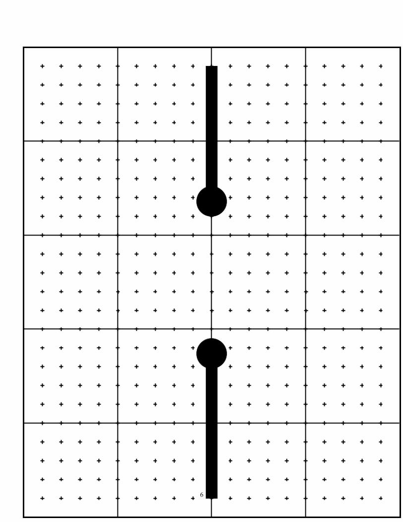
Procedure 1. Mapping equipotentials Tape one carbonised sheet on the cork board and apply 12V across the electrodes

using the DC power supply. Connect the grounded lead of the voltmeter to the grounded electrode and the other lead to the needle probe. Use the probe to identify points on the paper at 2, 4, 6, 8, and 10V. Identify five or six points for each choice of voltage. Mark the points on a template on which the electrode configuration has been copied. Draw and label lines of equal potentials. Repeat using the other two carbonized sheets.

2. Field lines. On each template, draw a number of field lines extending from one electrode to the other.

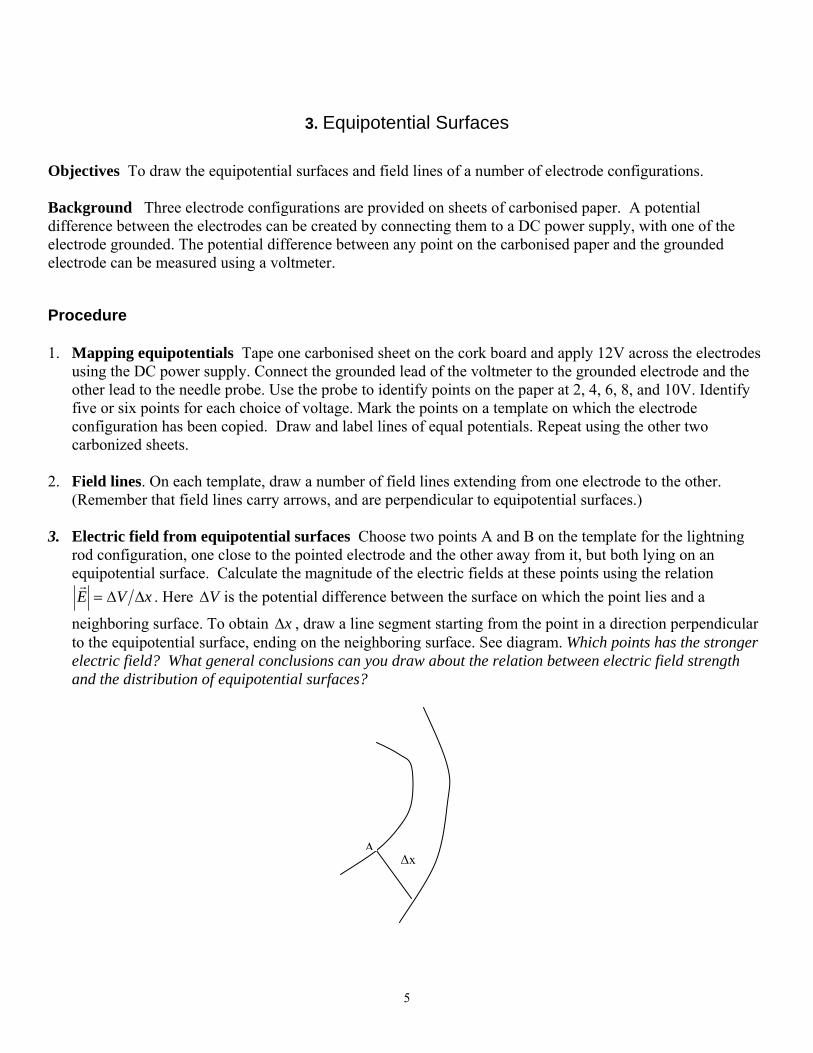
(Remember that field lines carry arrows, and are perpendicular to equipotential surfaces.) 3. Electric field from equipotential surfaces Choose two points A and B on the template for the lightning

rod configuration, one close to the pointed electrode and the other away from it, but both lying on an equipotential surface. Calculate the magnitude of the electric fields at these points using the relation

xVE ΔΔ=r

. Here VΔ is the potential difference between the surface on which the point lies and a

neighboring surface. To obtain xΔ , draw a line segment starting from the point in a direction perpendicular to the equipotential surface, ending on the neighboring surface. See diagram. Which points has the stronger electric field? What general conclusions can you draw about the relation between electric field strength and the distribution of equipotential surfaces?

AΔx

6

7

8

9

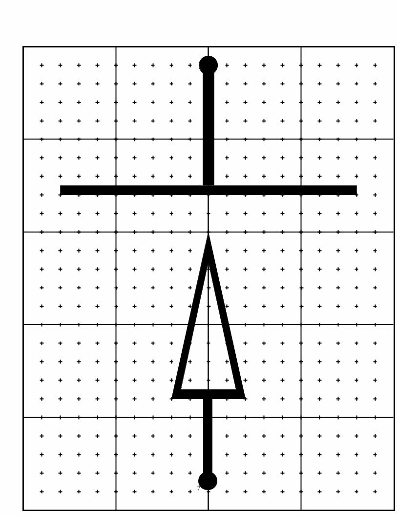
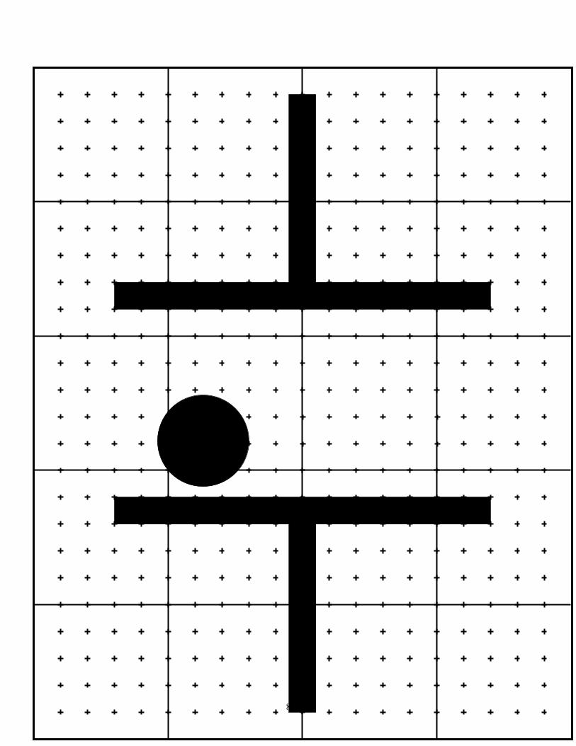
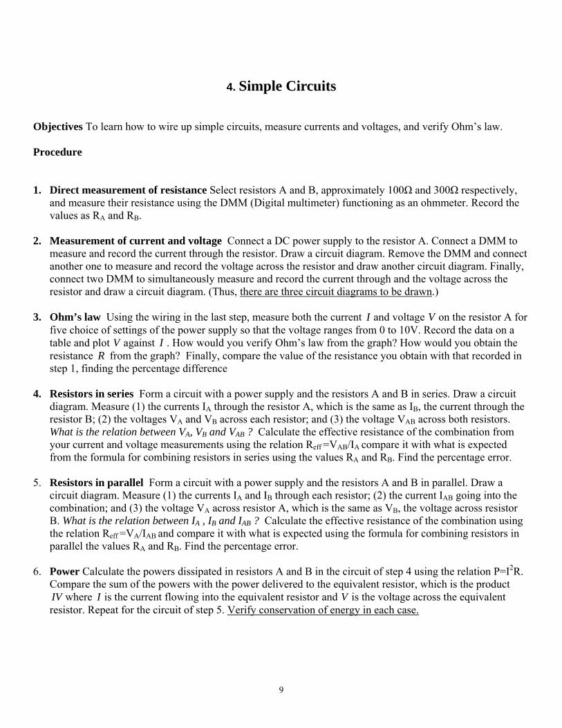
4. Simple Circuits Objectives To learn how to wire up simple circuits, measure currents and voltages, and verify Ohm’s law. Procedure 1. Direct measurement of resistance Select resistors A and B, approximately 100Ω and 300Ω respectively,

and measure their resistance using the DMM (Digital multimeter) functioning as an ohmmeter. Record the values as RA and RB.

2. Measurement of current and voltage Connect a DC power supply to the resistor A. Connect a DMM to

measure and record the current through the resistor. Draw a circuit diagram. Remove the DMM and connect another one to measure and record the voltage across the resistor and draw another circuit diagram. Finally, connect two DMM to simultaneously measure and record the current through and the voltage across the resistor and draw a circuit diagram. (Thus, there are three circuit diagrams to be drawn.)

3. Ohm’s law Using the wiring in the last step, measure both the current I and voltage V on the resistor A for

five choice of settings of the power supply so that the voltage ranges from 0 to 10V. Record the data on a table and plot V against I . How would you verify Ohm’s law from the graph? How would you obtain the resistance R from the graph? Finally, compare the value of the resistance you obtain with that recorded in step 1, finding the percentage difference

4. Resistors in series Form a circuit with a power supply and the resistors A and B in series. Draw a circuit

diagram. Measure (1) the currents IA through the resistor A, which is the same as IB, the current through the resistor B; (2) the voltages VA and VB across each resistor; and (3) the voltage VAB across both resistors. What is the relation between VA, VB and VAB ? Calculate the effective resistance of the combination from your current and voltage measurements using the relation Reff =VAB/IA compare it with what is expected from the formula for combining resistors in series using the values RA and RB. Find the percentage error.

5. Resistors in parallel Form a circuit with a power supply and the resistors A and B in parallel. Draw a

circuit diagram. Measure (1) the currents IA and IB through each resistor; (2) the current IAB going into the combination; and (3) the voltage VA across resistor A, which is the same as VB, the voltage across resistor B. What is the relation between IA , IB and IAB ? Calculate the effective resistance of the combination using the relation Reff =VA/IAB and compare it with what is expected using the formula for combining resistors in parallel the values RA and RB. Find the percentage error.

6. Power Calculate the powers dissipated in resistors A and B in the circuit of step 4 using the relation P=I2R.

Compare the sum of the powers with the power delivered to the equivalent resistor, which is the product IV where I is the current flowing into the equivalent resistor and V is the voltage across the equivalent resistor. Repeat for the circuit of step 5. Verify conservation of energy in each case.

10

5. Measurement of e/m Objective To measure the e/m for electrons from cyclotron motion Background An electron moving perpendicularly to a uniform magnetic field B travels in a circle of radius r given by

eBmvr =

where v is its velocity. If the electron has been accelerated from rest by a voltage V , its velocity can be obtained from the relation

eVmv =2

21

In both equations, the charge and mass of the electron occur in the combination me . Eliminating v from the above equation leads to the relation

22

2rB

Vme=

Thus me can be determined if rBV ,, are measured. In this experiment, a source of electrons is supplied from the filament circuit, which consists of a filament heated by the current from a power supply. The electrons are accelerated using the accelerating circuit, which applies a voltage across the filament and an anode using a high voltage power supply. The electrons then enter the evacuated space inside a glass tube filled with mercury vapor. The track they follow is made visible from ionisation of the mercury vapor. The tube is surrounded by a pair of Helmholtz coils, which produces a magnetic field equal to

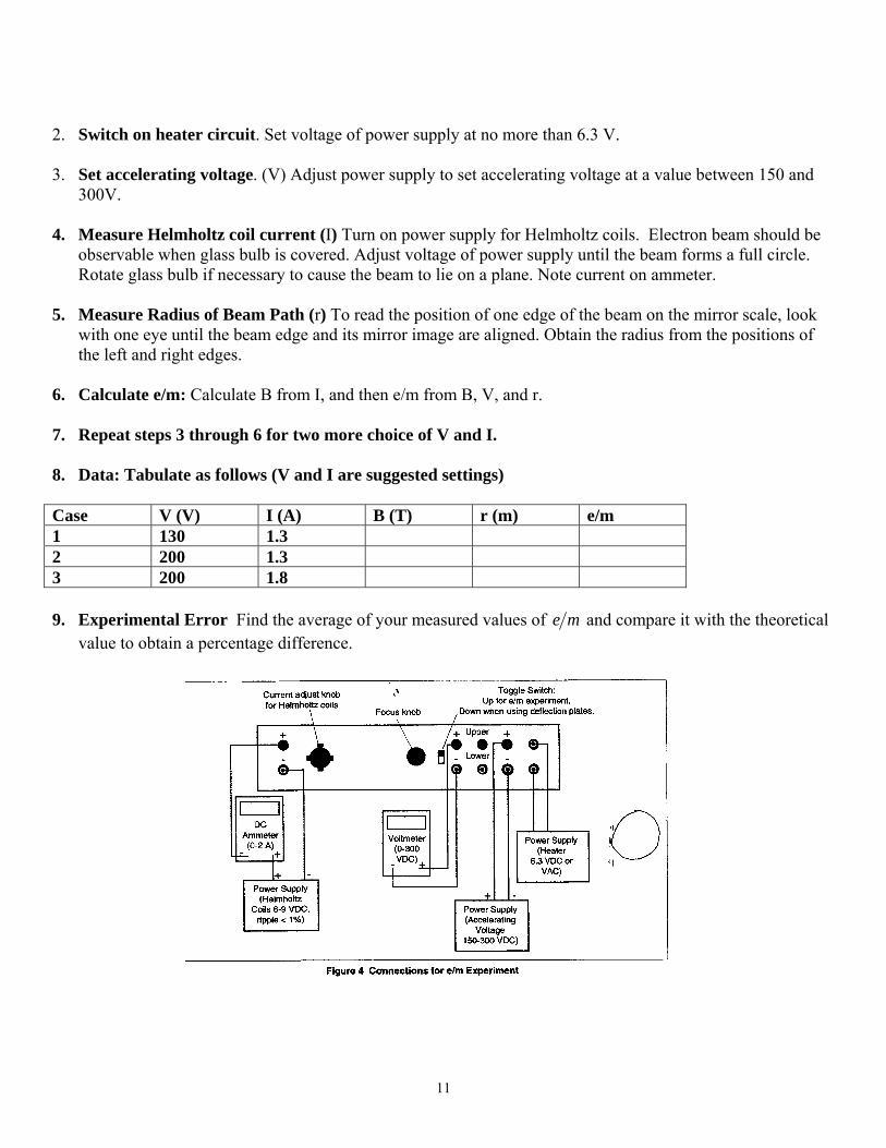
IB 41080.7 −×= in Tesla (T) when a current I (in ampere) flows through the coils. Procedure 1. Connect circuits as shown.

Toggle switch: up position Heater circuit: Power Supply set at 6.3V Helmholtz coil circuit: Ammeter connected. Power supply variable ( 6-9 V) Accelerating circuit: Voltmeter connected. Power supply variable (150-300 V)

11

2. Switch on heater circuit. Set voltage of power supply at no more than 6.3 V. 3. Set accelerating voltage. (V) Adjust power supply to set accelerating voltage at a value between 150 and

300V. 4. Measure Helmholtz coil current (I) Turn on power supply for Helmholtz coils. Electron beam should be

observable when glass bulb is covered. Adjust voltage of power supply until the beam forms a full circle. Rotate glass bulb if necessary to cause the beam to lie on a plane. Note current on ammeter.

5. Measure Radius of Beam Path (r) To read the position of one edge of the beam on the mirror scale, look

with one eye until the beam edge and its mirror image are aligned. Obtain the radius from the positions of the left and right edges.

6. Calculate e/m: Calculate B from I, and then e/m from B, V, and r. 7. Repeat steps 3 through 6 for two more choice of V and I. 8. Data: Tabulate as follows (V and I are suggested settings) Case V (V) I (A) B (T) r (m) e/m 1 130 1.3 2 200 1.3 3 200 1.8 9. Experimental Error Find the average of your measured values of me and compare it with the theoretical

value to obtain a percentage difference.

12

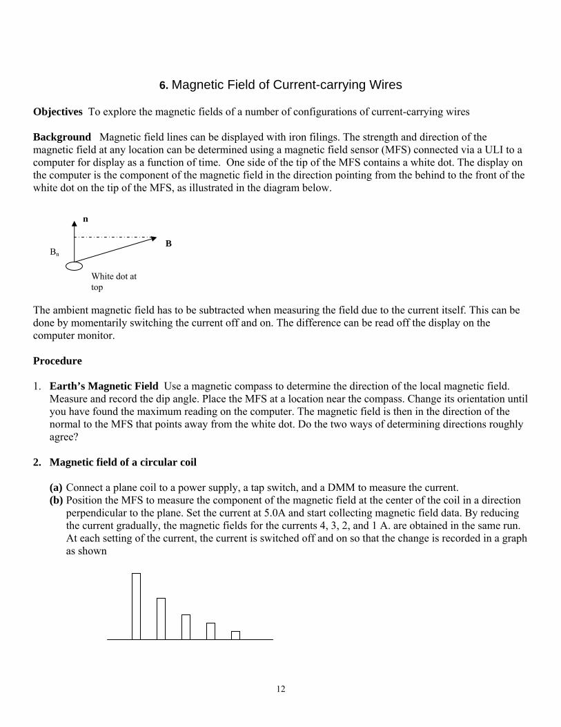
6. Magnetic Field of Current-carrying Wires Objectives To explore the magnetic fields of a number of configurations of current-carrying wires Background Magnetic field lines can be displayed with iron filings. The strength and direction of the magnetic field at any location can be determined using a magnetic field sensor (MFS) connected via a ULI to a computer for display as a function of time. One side of the tip of the MFS contains a white dot. The display on the computer is the component of the magnetic field in the direction pointing from the behind to the front of the white dot on the tip of the MFS, as illustrated in the diagram below.

The ambient magnetic field has to be subtracted when measuring the field due to the current itself. This can be done by momentarily switching the current off and on. The difference can be read off the display on the computer monitor. Procedure 1. Earth’s Magnetic Field Use a magnetic compass to determine the direction of the local magnetic field.

Measure and record the dip angle. Place the MFS at a location near the compass. Change its orientation until you have found the maximum reading on the computer. The magnetic field is then in the direction of the normal to the MFS that points away from the white dot. Do the two ways of determining directions roughly agree?

2. Magnetic field of a circular coil

(a) Connect a plane coil to a power supply, a tap switch, and a DMM to measure the current. (b) Position the MFS to measure the component of the magnetic field at the center of the coil in a direction

perpendicular to the plane. Set the current at 5.0A and start collecting magnetic field data. By reducing the current gradually, the magnetic fields for the currents 4, 3, 2, and 1 A. are obtained in the same run. At each setting of the current, the current is switched off and on so that the change is recorded in a graph as shown

B

n

Bn

White dot at top

13

Plot the magnetic field of the current against the current. Can you conclude that the magnetic field is proportional to the current? (c) If you look at the coil from a position where the current is counter clockwise, is the direction of the

measured magnetic field pointing toward or away from you? Does this agree with what you expect?

3. Magnetic field of a straight wire

1. Display field lines Connect a long straight wire to a power supply and a switch. The wire pierces through a piece of horizontal card board paper. Sprinkle iron filings on the paper around the wire. Pass a current through the wire. Lightly tap on the paper and observe the pattern formed by the filings.

2. Measure field strength

(a) Azimuthal dependence Use the MFS to measure both the directions and the magnitudes of the

magnetic field on four locations on the paper around the wire but at the same distance of about 1cm from the wire. You will need to switch the current on and off to subtract out the Earth’s field as in step 2. What conclusions can you draw? How is the direction of the magnetic field related to the direction of the current?

(b) Radial dependence Measure the magnetic fields on the paper at four or five locations along a

direction that goes out radially from the wire. Plot the magnetic field strength against r/1 where r is the distance between the location and the wire. Draw your conclusions based on the graph.

4. Solenoid Display the field lines inside a current-carrying solenoid using iron filings on a thin strip of paper

inserted into the solenoid. Do the same in the region immediately outside the two ends of the solenoid. (You can accomplish both tasks by cutting the paper into a T shape.) Sketch the field lines based on these observations.

Equipment: A straight wire A multiloop coil A solenoid A compass A lambda power supply A high current power supply A tap switch A 5-Ohm rheostat One DMM Iron filings Index cards Computer A magnetic field sensor

14

7. Ray Tracing Objectives To study the laws of reflection and refraction by tracing rays. Background The line of sight of a small object is the straight line from the object that goes through one eye. It can be identified by positioning two pins between the object and the eye so that they are all lined up. A ray can be identified by drawing a straight line on a piece of paper taped on a cork board and inserting two pins on the line. Procedure

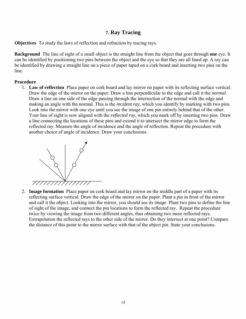
1. Law of reflection Place paper on cork board and lay mirror on paper with its reflecting surface vertical. Draw the edge of the mirror on the paper. Draw a line perpendicular to the edge and call it the normal. Draw a line on one side of the edge passing through the intersection of the normal with the edge and making an angle with the normal. This is the incident ray, which you identify by marking with two pins. Look into the mirror with one eye until you see the image of one pin entirely behind that of the other. Your line of sight is now aligned with the reflected ray, which you mark off by inserting two pins. Draw a line connecting the locations of these pins and extend it to intersect the mirror edge to form the reflected ray. Measure the angle of incidence and the angle of reflection. Repeat the procedure with another choice of angle of incidence. Draw your conclusions.

2. Image formation Place paper on cork board and lay mirror on the middle part of a paper with its

reflecting surface vertical. Draw the edge of the mirror on the paper. Plant a pin in front of the mirror and call it the object. Looking into the mirror, you should see its image. Plant two pins to define the line of sight of the image, and connect the pin locations to form the reflected ray. Repeat the procedure twice by viewing the image from two different angles, thus obtaining two more reflected rays. Extrapolation the reflected rays to the other side of the mirror. Do they intersect at one point? Compare the distance of this point to the mirror surface with that of the object pin. State your conclusions.

15

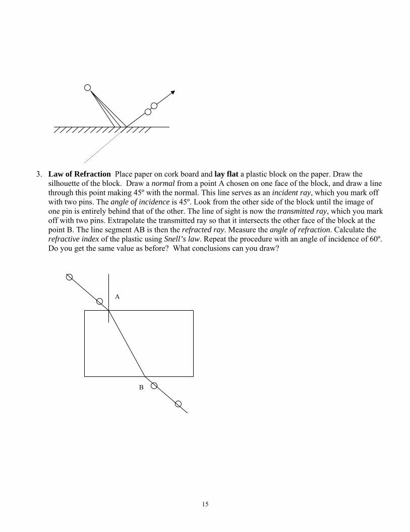
3. Law of Refraction Place paper on cork board and lay flat a plastic block on the paper. Draw the

silhouette of the block. Draw a normal from a point A chosen on one face of the block, and draw a line through this point making 45º with the normal. This line serves as an incident ray, which you mark off with two pins. The angle of incidence is 45º. Look from the other side of the block until the image of one pin is entirely behind that of the other. The line of sight is now the transmitted ray, which you mark off with two pins. Extrapolate the transmitted ray so that it intersects the other face of the block at the point B. The line segment AB is then the refracted ray. Measure the angle of refraction. Calculate the refractive index of the plastic using Snell’s law. Repeat the procedure with an angle of incidence of 60º. Do you get the same value as before? What conclusions can you draw?

A

B

16

8. Image Formation with a Convex Lens Background The lens equation

fdd io

111=+

relates the object distance od , the image distance id , and the focal length f of a single lens. For a convex lens, when the object is far away, the approximate relation odf ≈ holds. The magnification m , defined by the ratio of the image to the object sizes,

o

i

hh

m =

is also related to these distances by

o

i

dd

m −=

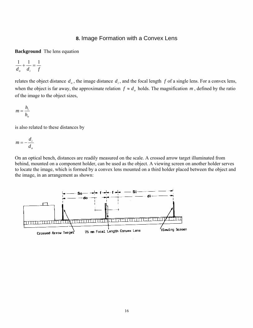
On an optical bench, distances are readily measured on the scale. A crossed arrow target illuminated from behind, mounted on a component holder, can be used as the object. A viewing screen on another holder serves to locate the image, which is formed by a convex lens mounted on a third holder placed between the object and the image, in an arrangement as shown:

17

Procedure 1. The Focal Length Determine the focal length of a thin lens by locating the image of a far away object. This can be accomplished by locating the image as the smallest spot when the separation between the object and the lens is as long as allowed by the optical bench.

mf = 2. Validity of the Thin Lens Equation Determine the locations of the images formed by the lens of objects at the following distances from the lens: 40cm, 30cm, 20cm, 10cm. Measure the size of the object oh . Also measure the size of the image in each case. Verify the thin lens equation by completing the table below:

mmho =

)(mdo ( )mdi ( )mhi io dd 11 + f1 oi hh oi dd− It is expected that the 4th and 5th columns, and the 6th and the 7th columns, should be equal. 3. Application of Lens Equation Calculate the location and magnification of the image of an object at a distance of 15cm from the lens. Determine the same quantities using ray tracing on a graph paper. Verify these results by locating the image on the optical bench. 4. Virtual Image Calculate the location and magnification of the image if the object is at 5cm from the lens. Can the image be located using the screen? Explain why or why not.

18

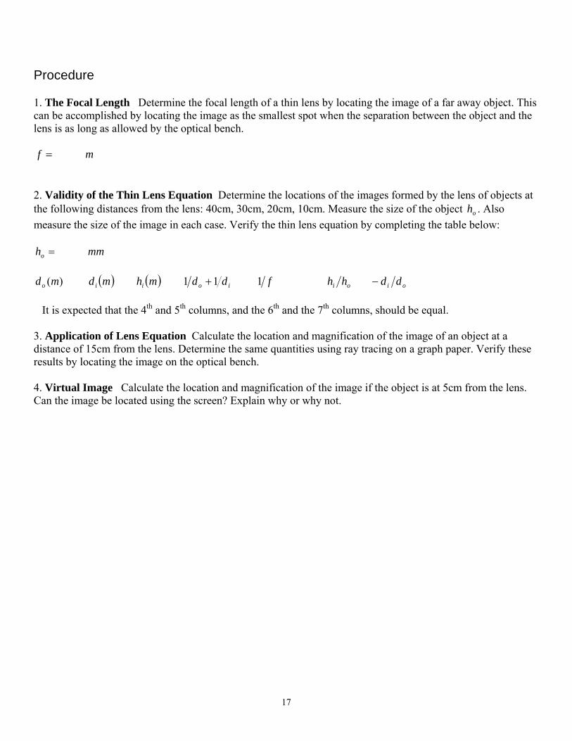
9. Interference and Diffraction Using Laser Background Single Slit Diffraction When a plane light wave of wavelength λ is incident perpendicularly on a single slit with width w , it spreads out on the other side due to diffraction. The intensity depends on the direction of the transmitted ray, which is identified by the angle θ that the ray makes with the normal to the plane of the slit as shown. The angle θ is usually small, and is conveniently measured in radian.

The intensity is largest at 0=θ , and is equal to zero when θ satisfies the condition

wnnλθ =

where K,2,1,0 ±±=n . . Between nθ and 1+nθ , the intensity rises and falls, showing a diffraction peak. The central diffraction peak is between 1−θ and 1θ ,, so that

angular width of central diffraction peak wλ2

=

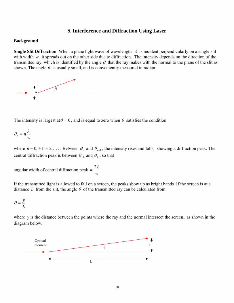
If the transmitted light is allowed to fall on a screen, the peaks show up as bright bands. If the screen is at a diatance L from the slit, the angle θ of the transmitted ray can be calculated from

Ly

=θ

where y is the distance between the points where the ray and the normal intersect the screen., as shown in the diagram below.

w θ

L

θ

Optical element y

19

Double Slit Interference If a double slit with infinitely small slit width is used, and the slit separation is d , the transmitted wave in the direction θ with the normal shows a maximum whenever

dn λθ = L,2,1,0 ±±=n

and complete darkness when

dn λθ ⎟

⎠⎞

⎜⎝⎛ +=

21

The angular separation between successive dark spots (or fringes) is therefore given by

dλθ =Δ

Taking the finiteness of the slit width w into account, the single slit diffraction central peak would show a number of dark fringes. Diffraction Grating The diffraction grating contains a large number of slits that are very close together. The spacing is characterized by the grating constant, which is the number of slits per unit length. If d is once again to denote the distance between neighboring slits, it is no longer much smaller than the wavelength λ so that small angle approximation can no longer be used. The condition for a direction to show maximum intensity is now

λθ nd =sin and the angle θ can be determined from the image on the screen using

Ly

=θtan

In this experiment, a laser beam is used as the monochromatic light source. On the diffraction plate, the following elements will be used: A: single slit ( mmw 04.0= ) B: single slit ( mmw 08.0= ) D: double slit ( mmwmmd 04.0125.0 == ) E: double slit ( mmwmmd 04.0250.0 == ) The grating plate contains 5276 lines per cm.

20

Procedure Attach diffraction plate and white screen on separate stands, and place stands and laser on optical bench. .

1. Single Slit Diffraction

(a) Place diffraction plate and screen 30 cm apart and train laser beam on element A on the diffraction plate. Observe intensity pattern on the screen. How many diffraction peaks do you see?

(b) Measure the width of the central diffraction peak on the screen, and determine the wavelength of

the laser.

Distance between single slit and screen =L Half width of central diffraction peak =y Angular width of half peak in radian =1θ Slit width =w Wavelength =λ

(c) Train laser beam on element B on diffraction plate and observe intensity pattern on screen. How

does the width of the central peak depend on the slit width?

2. Double Slit Interference

(a) Train laser beam on element D and observe intensity pattern on screen. How many dark fringes do you see inside of the single slit diffraction central peak? Fringes can be made more discernable by slanting the screen.

(b) Calculate number of dark fringes in (a) from theory:

Slit separation =d Wavelength (from part 1) =λ Angular separation between dark fringes in radian =Δθ Angular width of central peak (from part 1) in radian =12θ Number of dark fringes =

Does this number depend on wavelength? (c) Train laser beam on element E and observe intensity pattern. How does the spacing between dark

fringes depend on the separation between the slits?

21

3. Diffraction Grating. Mount diffraction grating on stand and place it 10 cm from the screen on the optical bench. Train laser beam on grating and locate central bright spot and a fainter spot that corresponds to the first order maximum intensity. Measure the distance between the faint spot and the central spot and hence calculate the wavelength of the laser.

Separation between neighboring slits =d Distance between grating and screen =L Distance between central and first order bright spots on screen =y Direction of first order bright spot from normal =)deg( reeinθ Wavelength =λ

22

10. Photoelectric Effect Background Photons can dislodge electrons from a metal and impart kinetic energy to them. The maximum kinetic energy of these electrons released from the metal surface, called the photocathode, is given by the equation

WhfK −=max where f is the frequency of the photon, W is the work function of the metal, and h is Planck’s constant. Traveling in the evacuated space in a tube from the cathode to the anode, these electrons form a photocurrent. The current can be reduced by biasing the anode at a lower potential than the cathode. It can be completely stopped if the potential difference is SV so that

maxKeVS = where e is the electron charge. The quantity SV , called the stopping potential, can be readily measured. Combining the two equations leads to the equation

eWf

ehVS −=

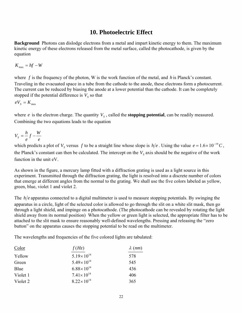
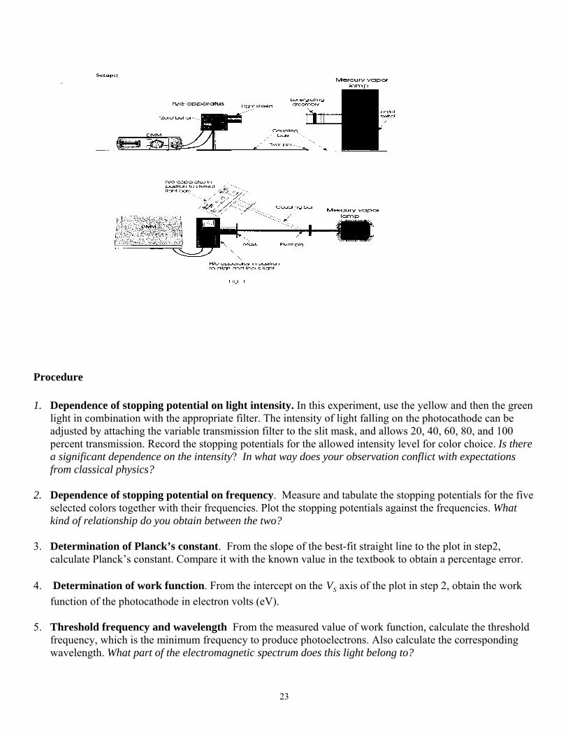
which predicts a plot of SV versus f to be a straight line whose slope is eh . Using the value Ce 19106.1 −×= , the Planck’s constant can then be calculated. The intercept on the SV axis should be the negative of the work function in the unit eV. As shown in the figure, a mercury lamp fitted with a diffraction grating is used as a light source in this experiment. Transmitted through the diffraction grating, the light is resolved into a discrete number of colors that emerge at different angles from the normal to the grating. We shall use the five colors labeled as yellow, green, blue, violet 1 and violet 2. The eh apparatus connected to a digital multimeter is used to measure stopping potentials. By swinging the apparatus in a circle, light of the selected color is allowed to go through the slit on a white slit mask, then go through a light shield, and impinge on a photocathode. (The photocathode can be revealed by rotating the light shield away from its normal position) When the yellow or green light is selected, the appropriate filter has to be attached to the slit mask to ensure reasonably well-defined wavelengths. Pressing and releasing the “zero button” on the apparatus causes the stopping potential to be read on the multimeter. The wavelengths and frequencies of the five colored lights are tabulated: Color )(Hzf )(nmλ

Yellow 141019.5 × 578 Green 141049.5 × 545 Blue 141088.6 × 436 Violet 1 141041.7 × 406 Violet 2 141022.8 × 365

23

Procedure 1. Dependence of stopping potential on light intensity. In this experiment, use the yellow and then the green

light in combination with the appropriate filter. The intensity of light falling on the photocathode can be adjusted by attaching the variable transmission filter to the slit mask, and allows 20, 40, 60, 80, and 100 percent transmission. Record the stopping potentials for the allowed intensity level for color choice. Is there a significant dependence on the intensity? In what way does your observation conflict with expectations from classical physics?

2. Dependence of stopping potential on frequency. Measure and tabulate the stopping potentials for the five

selected colors together with their frequencies. Plot the stopping potentials against the frequencies. What kind of relationship do you obtain between the two?

3. Determination of Planck’s constant. From the slope of the best-fit straight line to the plot in step2,

calculate Planck’s constant. Compare it with the known value in the textbook to obtain a percentage error. 4. Determination of work function. From the intercept on the SV axis of the plot in step 2, obtain the work

function of the photocathode in electron volts (eV). 5. Threshold frequency and wavelength From the measured value of work function, calculate the threshold

frequency, which is the minimum frequency to produce photoelectrons. Also calculate the corresponding wavelength. What part of the electromagnetic spectrum does this light belong to?