PHY 252 Lab 3: Millikan oil drop/charge of electron

Fall 2008

The purpose of this experiment is to measure the smallest unit into which electric charge canbe divided, that is, the charge e of an electron. The method is essentially the one employed byR.A. Millikan in 1910. The essence of the experiment is to measure the terminal velocity of afalling droplet to measure its radius r and thus mass m, and then to suspend the droplet with anelectric field so that one can measure its charge q from qE = mg. By repeating many measure-ments, Millikan was able to show that charge comes in integer multiples of a fundamental value.Millikin used oil droplets for his experiments; you’ll use micrometer-scale polystyrene spheresinstead.

When objects move through a fluid, one can have either turbulent or laminar flow. The dividingline between the two is given by the Reynolds number R = !vL/", which is the ratio of inertialto viscuous forces found from the fluid density !, dynamic viscosity " (some books use µ torepresent this), velocity v, and characteristic length L of the object moving through the fluid. LowReynolds number (R <! 30) corresponds to laminar flow, while high Reynolds number (R >! 3000)corresponds to turbulent flow. In the low Reynolds number limit (appropriate for micrometer-scaleobjects moving through air), the drag forces on a sphere with radius r is given by

Fd = 6#"rv. (1)

In the high Reynolds number limit (appropriate for people and cars moving through air), dragforces are given by

Fd =1

2!v2ACd (2)

where A is the area of the object and Cd is a coefficient of drag which is typically in the range 0.2–1. The appearance of (1/2)!v2 tells you that the kinetic energy of the air pushed aside in turbulentflow is what determines the drag force. In the low Reynolds number limit (and neglecting thebuoyant force of air, since its density is a thousand times lower than that of polystyrene), terminalvelocity vT is reached when Fd = mg so that there is no net acceleration; from this fact, Eq. 1, andm = (4/3)#r3!, one can find the radius r of the sphere to be

r2 =9"vT

2!g(3)

and its mass to bem =

4

3(9

2)3/2(

"vT

g)3/2 1

"!. (4)

1

Air at 25!C has a dynamic viscosity of 1.85# 10"5 N·s/m2, and polystyrene has a density of 1050kg/m3, so for the polystyrene spheres used in this experiment you can readily determine their massfrom their terminal velocity. Then, if you create an electric field E = V/d from a voltage Vapplied to plates a distance d apart, and thereby suspend a sphere by counteracting gravity, you canmeasure its charge from qE = mg or

q =mg

E=

mgd

V. (5)

1 ApparatusA schematic of the apparatus is shown in Fig. 1, and a photograph is shown in Fig. 2. In the closedchamber, a uniform electric field E = V/d can be applied between two capacitor plates d = 0.40cm apart by adjusting a voltage V using the right-hand knob on the power supply shown in Fig. 3.The chamber is illuminated by a small lamp. Charged spheres (a suspension of latex in water andalcohol) can be blown into the chamber through a tubing and a nozzle, and be viewed there througha telescope with a calibrated scale (the spacing of graduations is 0.5 mm). Note that the telescopegives an inverted image.

1. Turn on the light and focus the telescope on the end of the nozzle which is used to blowspheres into the chamber. Then pull the nozzle back out of the field of view. Spheres cannow be blown into the chamber by squeezing the rubber bulb.

2. Blow some spheres into the chamber and watch them (they will look tiny). They will quicklyreach terminal velocity vT and should all be falling at the same rate in the absence of anelectric field. Measure this velocity by timing the travel of particles over a known distancewith a stop watch. Repeat several times until you get a set of consistent values. Calculatethe mass from the average terminal velocity.

3. Blow more spheres into the chamber and watch them falling. Now turn up the electric field.You will see them reverse direction and reach a new terminal velocity, which now dependson their charge q. Since you want to measure small charges, select one that is least affectedby the E field and adjust the voltage V to hold it stationary. Write down the value of V(which determines E), and repeat the measurement 20 or more times, trying to find sphereswith slightly different charges.

4. Calculate q for each sphere, using Eqs. 4 and 5.

Now that you have a set of qi measurements with i = 1, 2, . . . , N , you should make a histogramof your measurements. On the horizontal axis, pick intervals of charge q (for example, q = 0 to0.2# 1019C, 0.2 to 0.4# 10"19C, and so on), and then within each bin plot on the vertical axis thenumber of measurements that fall within that q range. Ideally you’ll get one or more peaks aroundparticular values of q! Assign successive integers k = 1, 2, . . . to these peaks. Now plot q versus kfor all of your data. Since we expect the relationship q = ke, the slope of a least squares fit shouldgive you the electron charge e!

2

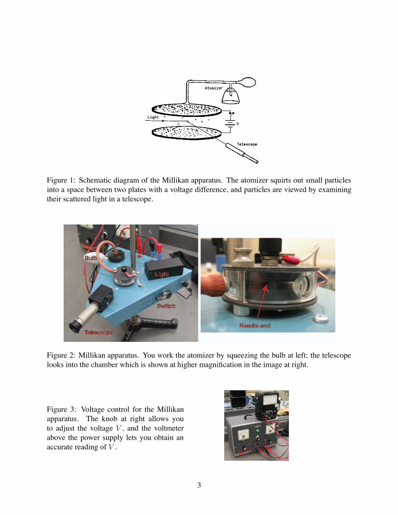
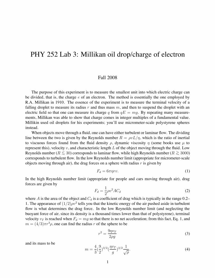
Figure 1: Schematic diagram of the Millikan apparatus. The atomizer squirts out small particlesinto a space between two plates with a voltage difference, and particles are viewed by examiningtheir scattered light in a telescope.

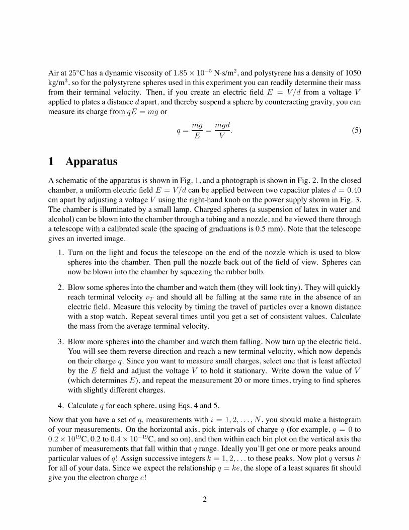
Figure 2: Millikan apparatus. You work the atomizer by squeezing the bulb at left; the telescopelooks into the chamber which is shown at higher magnification in the image at right.

Figure 3: Voltage control for the Millikanapparatus. The knob at right allows youto adjust the voltage V , and the voltmeterabove the power supply lets you obtain anaccurate reading of V .

3