Performance prediction of a constructed wetland wastewater

1 1, 2 & V. Popov1

1Wessex Institute of Technology, Southampton, UK 2

(Central University), New Delhi India

Abstract

performance of a constructed wetland wastewater treatment plant (CWWTP). The model assesses the Biochemical Oxygen Demand (BOD) concentration at outlet of a treatment plant. Training of ANN models was based on experimental results of a pilot plant study in India. The data used in this work were obtained under various hydraulic and BOD loading. Regular records of BOD were made at inlet, and outlet levels through various stages of the treatment process for over 18 months. The ANN-based models were found to provide an efficient and a robust tool in predicting CWWTP performance. Keywords: neural networks, constructed wetland, model studies, prediction, optimization, biochemical oxygen demand.

1 Introduction

The proper operation and management of constructed wetland wastewater treatment plants (CWWTP) is receiving attention because of the rising concern about environmental issues and growing importance of sustainable and natural wastewater treatment techniques. Improper design and operation of a CWWTP may cause serious environmental and public health implications, as its effluent may contaminate receiving water body, causing severe aquatic pollution and spread various water born diseases. For proper design and assessment of quality of non-conventional wastewater treatment and thereafter to conserve the receiving water bodies, reliable prediction of effluent from Constructed Wetland (CW) is essential. A better control can be achieved by developing a

www.witpress.com, ISSN 1743-3541 (on-line)

© 2006 WIT PressWIT Transactions on Ecology and the Environment, Vol 92,

Waste Management and the Environment III 143

V. Tomenko , S. Ahmed

Artificial neural network (ANN) models were developed to predict the

Department of Civil Engineering, Jamia Millia Islamia

wetland wastewater treatment plant Performance prediction of a constructed

doi:10.2495/WM060161

mathematical tool for predicting the plant performance based on past observations of certain key parameters. However, modeling a CWWT is a difficult task due to the complexity of the treatment processes. The complex physical, biological and chemical processes involved in constructed wetland treatment process exhibit non-linear behaviors, which are difficult to describe by linear mathematical models. This paper presents predictive models based on the concept of neural networks (NN). Artificial intelligence concepts have been successfully used in a range of engineering, environmental, and financial problems [1, 2]. The NN-based model that was applied to a pilot plant study of CW in India have performed consistently well in the face of varying accuracy and size of input data. Using these models, the planner and decision maker can easily make assessment of the expected plant effluent.

2 Constructed wetland pilot plant and experimental set up

Wetlands are considered as low-cost alternatives for treating municipal, industrial, and agricultural effluents. Constructed wetlands (CW) are preferred because of low maintenance, shock loading absorbance capacity and less energy consumption [3]. They may be classified as surface flow marshes, vegetated subsurface flow beds, submerged aquatic beds, and floating leaved aquatics [4] This new developing technology may offer a low cost and low maintenance alternative for treatment of domestic wastewater which is especially suitable for developing countries [5, 6]. The scheme of the units designed in New Delhi is presented in Fig. 1.

Figure 1: Pilot plant scheme.



144 Waste Management and the Environment III

Construction was completed in August 2001. The initial sampling started after eight months i.e. April –2002 giving sufficient time for full growth of reeds since wetlands typically require a few months for vegetation and bio-film establishment according to [7]. Sizing of the wetland units was done by using basic relationship for plug flow reactor for the BOD loading as recommended by [8]:

( )0ln lndQ C CtA

K−

= (1)

where A is the plane area of the wetland unit, (m2), K is the specific removal rate constant for given constituent at 200C, (d-1), dQ is the average flow rate of wastewater (m3 d-1), 0C is the average BOD5 of the influent (mg/l) and tC is the average BOD5 of the effluent (mg/l). Each unit has length = 6.6 m, width = 5.3 m. and depth = 0.6m. Two parallel Subsurface Horizontal Flow Constructed wet land units A and B with same filler material were used in this study. The inlet zone (first 100 cm) of unit B has coarse sand filler matrix. Both were planted with Phragmites australis. Different hydraulic loading starting from 34 l/m2/d to 200l/m2/d were used in the experiments. The BOD loading of the pilot plant was varied from 45 mg/l to 1580 mg/l, so that it can be tested for wide range of conditions. The flow meters were provided before the inlet zone to record the average flow rate and total quantity of waste-water feeded in each bed. All precautions were taken for equal distribution of wastewater in each of the CW beds. Five different triplicate samples including three intermediate were collected for set of parameters. Intermediate samples were collected from different ports at downstream distance of 3.15 m, 4.15 m and 5.15 m respectively. Acrylic sheets of 45 cm height were embedded up to 30 cm in the soil filter at inlet zone to avoid any over flow condition in CWs. Wastewater influent and effluent from the CW units were monitored and recorded after giving at least 15 days of acclimatization period to the CW. After fifteenth day, five daily samples were taken for given hydraulic and organic loading and mean values were obtained. In situ measurements for temperature and pH were also recorded at the influent, effluent and intermediate sampling points. The wastewater samples were not collected simultaneously but after giving due consideration of lack time for different hydraulic loading. Samples were analyzed for Chemical Oxygen Demand (COD), Biochemical Oxygen Demand (BOD), Phosphate (PO4) Faceal Coliform (FC) and Total Coliform (TC). All these analyses were conducted in accordance with [9]. In this study only BOD values were considered for development of ANN model.

3 Neural network modelling

During several last decades neural networks have been successfully applied for prediction and pattern recognition tasks. Their potential is especially high for the systems with complex non-linear behavior, when the laws governing the system are not known or poorly understood. Artificial neural networks are superior to




other computational formalisms in the case of noisy and ill-defined data, massively parallel computation, collective effects and signal dynamics [10]. There is a wide variety of wastewater treatment problems, where neural networks have been applied successfully, including modelling of the physicochemical water treatment process [11], prediction of wastewater treatment plant performance [12], photocatalytic treatment of waste waters [8] etc. The performance of the network strongly depends on the choice of process variables. The data available is also of great importance, especially in terms of representing the domain of experiment. Another important point is data preprocessing. Usually, the range of model variables varies and, therefore, some data preprocessing technique should be utilized. The most widely applied NN for modeling of steady-state systems are of feed-forward type. In such networks, the signal propagates in one direction via weighted connections between neurons of different layers (Fig. 2). The network model includes three layers of neurons: input, hidden and output layer. The neurons of input layer do not perform any calculations; they just store the input variables and propagate them to neurons of hidden layer. Each neuron of hidden and output layers (Fig. 3) calculates the weighted sum of inputs plus bias as follows:

∑=

+=N

jijjii xwu

1, θ (2)

Figure 2: Structure of feed-forward artificial neural network.




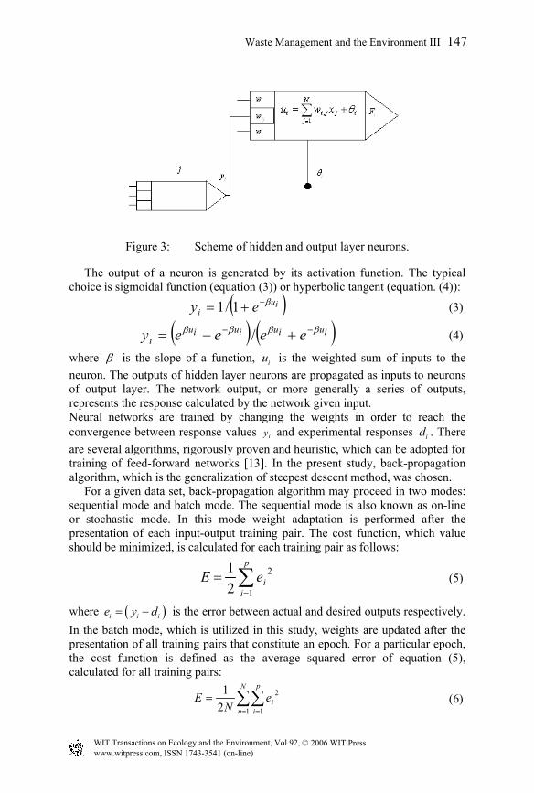
Figure 3: Scheme of hidden and output layer neurons.

The output of a neuron is generated by its activation function. The typical choice is sigmoidal function (equation (3)) or hyperbolic tangent (equation. (4)):

( )iui ey β−+= 1/1 (3)

( ) ( )iuiuiuiui eeeey ββββ −− +−= / (4)

where β is the slope of a function, iu is the weighted sum of inputs to the neuron. The outputs of hidden layer neurons are propagated as inputs to neurons of output layer. The network output, or more generally a series of outputs, represents the response calculated by the network given input. Neural networks are trained by changing the weights in order to reach the convergence between response values iy and experimental responses id . There are several algorithms, rigorously proven and heuristic, which can be adopted for training of feed-forward networks [13]. In the present study, back-propagation algorithm, which is the generalization of steepest descent method, was chosen. For a given data set, back-propagation algorithm may proceed in two modes: sequential mode and batch mode. The sequential mode is also known as on-line or stochastic mode. In this mode weight adaptation is performed after the presentation of each input-output training pair. The cost function, which value should be minimized, is calculated for each training pair as follows:

∑=

=p

iieE

1

2

21

(5)

where ( )i i ie y d= − is the error between actual and desired outputs respectively. In the batch mode, which is utilized in this study, weights are updated after the presentation of all training pairs that constitute an epoch. For a particular epoch, the cost function is defined as the average squared error of equation (5), calculated for all training pairs:

∑∑= =

=N

n

p

iie

NE

1 1

2

21

(6)




The objective of the learning process is to adjust the free parameters (weights, biases) of the network to minimize E. In the process of learning, the adjustments of the weights are calculated for each training pair according to delta rule [14]:

ji

zji w

Ew,

, ∂∂

−=∆ η (7)

where η is the learning-rate parameter, E is calculated by equation (5). The arithmetic mean of individual adjustments over the learning set gives estimate of the change that would minimize the cost function E and the weights are updated as follows:

( ) ( ) zji

zji

zji wtwtw ,,, 1 ∆+=+ (8)

For the neurons of output layer, the adjustments of weights are calculated in a straightforward manner:

( ) ( ) 11

,,,

−− ′−=′−=∂∂

∂∂

∂∂

∂∂

−=∂∂

−=∆ zjiii

zjiiiz

ji

i

i

i

i

i

iz

ji

zji yuyeyuye

wu

uy

ye

eE

wEw ηηηη (9)

If neuron j is located in the hidden layer z of the network, there is no specified desired response for that neuron. Therefore, the error for such neuron is determined with the help of error signals of neurons of output layer. Taking into account:

( ) 1,

1

111

11

1

1

1

11

1 )( +

=

+++

=+

+

+

+

+=

+ ∑∑∑ ′−=∂∂

∂∂

∂∂

=∂∂

=∂∂ z

ji

p

i

zi

zii

zi

p

izi

zi

zi

zi

zi

ip

izi

izj

wuydyxu

uy

yE

xE

yE (10)

Adjustments of weights of neurons of hidden layer can be calculated in the following way:

( )

′−′=

∂

∂

∂

∂

∂∂

−=∂∂

−=∆ +

=

+++∑ 1,

1

111

,,, )()( z

ji

p

i

zi

zii

zi

zi

zj

zjz

ji

zj

zj

zj

zj

zij

zij wuydyxuy

w

u

u

y

yE

wEw ηη (11)

During the learning process, not only weights and biases are varied, but also the number of neurons of hidden layer, learning-rate parameter (η ) and even the structure of the network itself (some connections can be eliminated). Generally, the number of neurons of hidden layer should be reduced to prevent network from over-fitting. On the other hand, elimination of too many neurons leads to reducing the performance of the network. Moreover, convergence of the solution is extremely sensitive to the adequate choice of η [13]. In general, back-propagation algorithm cannot be shown to converge. Therefore, the typical stopping criteria are the number of iterations or the sufficiently small gradient values [13].

4 Experimental results

NN model adopted contains three layers (input, hidden and output layers) as illustrated in Fig. 2. The aim of the learning procedure was to predict outBOD as a function of input variables. Six input variables were chosen:




1) inBOD , influent contamination (mg/l); 2) HL :, hydraulic Loading (l/m2/d); 3) OL :, organic loading (g/ m2/d); 4) t : temperature (0C); 5) v : velocity of the stream (m/s); 6) d : distance from the CWWTP influent (m).

The output variable (response) is the level of outBOD after treatment. Therefore, the output layer of the neural network includes one neuron. The distribution of the data pairs ( ) ( )( ), , , , , ,in outBOD HL OL t v d BOD into the learning set (LS) and test set (TS) was based on the experimental design and dataset properties. The LS and TS are comprised of 78 and 17 input-output pairs, respectively. The convergence criterion utilized was the cost function, defined by equation (6). Since the determination of the adequate number of neurons ( )m in hidden layer is important to prevent network from over-fitting, a number of learning procedures were performed in order to find the optimal combination of m and number of learning procedure epochs ( )NE . The number of neurons in the hidden layer varied between 6 and 14 and the number of epochs ranged from 500 to 1500. The values of cost function decreased as m increased from 6 to 12 for both data sets (LS and TS). For 12m > E calculated for TS increased (the network became over-fitted). According to the results, m was chosen to be 12 and 800NE = . When the cost function reached its minimum value, the weights of the network were fixed. Fig. 4 shows a comparison of calculated and experimental values of outBOD for both sets. The agreement between actual and predicted values is adequate for both LS and TS ( 2 0,997R = for LS and 2 0,995R = for TS).

Figure 4: Comparison of calculated and experimental values of BODout.




Given fixed values of , , , ,HL OL t v d , Figs. 5, 6 and 7 respectively show

outBOD as a function of distance from the influent of CW for three initial values of inBOD ( 45inBOD = , 156inBOD = , 784inBOD = ). The approximation is accurate; therefore, the neural network model is able to describe adequately the process kinetics under different conditions (initial values of input variables).

Figure 5: outBOD for inBOD = 45.


5 Conclusions

The neural network was adopted for prediction of constructed wetland contamination treatment performance for given hydraulic and BOD loading. The




NN model adequately describes the behavior of complex CWWTP within the range of different experimental conditions. Thus, if experimental data for a given system are available and cover the whole domain of interest, a simplified mathematical model of the wastewater treatment process may be obtained by utilizing feed-forward neural networks. Simulations based on the neural networks can then be performed to estimate the behavior of the system under different conditions.


This new developing technology may offer a low cost and maintenance to domestic wastewater treatment, which is especially suitable for developing countries.

References

[1] Jean P. Hybrid Fuzzy Neural Network for Diagnosis. Application of Anaerobic Treatment of Wine Distillery Waste Water Treatment in Fluidized Bed Reactor. Water Science Technology, Vol. 36 No 6-7 pp. 209-217, 1997.

[2] Mohammed F. Integrated Waste Water treatment Plant Performance Evaluation Using Artificial Neural Network. Water Science Technology, Vol. 40 No 7 pp. 55-65, 1999

[3] Vymazal J. The use of sub-surface constructed wetlands for wastewater treatment in the Czech Republic: 10 years experience. Ecological Engineering 18, pp. 633–646, 2002

[4] Reed SC, Middle brooks EJ, Crites RW. Natural systems for waste management and treatment. New York, NY: McGraw-Hill, 1988.

[5] SÇ Ayaz and I Akca. Treatment of wastewater by constructed wetland in small settlements. Water Science and Technology Vol. 41 No 1 pp 69–72, 2000.




[6] Ahmed Sirajuddin, Application of Root Zone Treatment System for Dairy Wastewater. Proceedings of the Mother Dairy International Conference on Constructed Wetlands for Waste Water Treatment in Tropical And Subtropical Regions. Anna University, Channai, December 11-13 2002.

[7] Billore SK, Singh N, Sharma JK, Dass P, Nelson RM. Horizontalsubsurf ace flow gravel bed constructed wetland with Phragmites karka in central India. Water Sci Technol 1999;40(3):163–71.

[8] Wood A. Constructed wetlands for wastewater treatment— engineering and design considerations. Proceedings of the International Conference on the use of Constructed Wetlands in Water Pollution Control. Cambridge, UK, 24–28 September 1990.

[9] APHA. Standard methods for the examination of water and wastewater, 19th ed. Washington, DC, USA: American Public Health Association/American Water Works Association Water Environment Federation; 1995

[10] Kohonen T. Self-Organizing Maps. Berlin: Springer, 1995. [11] Gob S., Oliveros E., Bossmann S. H., Braun A. M., Guardani R.,

Nascimento C.A.O. Modeling the kinetics of a photochemical water treatment process by means of artificial neural networks. Chemical Engineering and Processing 38, 373–382, 1999.

[12] Hamed M. M., Khalafallah M. G., Hassanien E. A. Prediction of wastewater treatment plant performance using artificial neural networks. Environmental Modelling & Software 19, 919–928, 2004

[13] S. Haykin, Neural Networks: a Comprehensive Foundation, 2nd Ed. Upper Saddle River, NJ: Prentice Hall, 1999.

[14] Widrow B., Hoff M.E. Adaptive switching circuits. In 1960 IRE WESCON Convention Record, pp. 96-104, 1960.




Documents

Performance prediction of a constructed wetland wastewater