Embed Size (px)
Citation preview

Performance Assessment of a Flow Balancing and WetlandTreatment System - Toronto,Ontario
2005


PERFORMANCE ASSESSMENT OF A FLOW BALANCING AND
WETLAND TREATMENT SYSTEM - TORONTO, ONTARIO
a report prepared by the
STORMWATER ASSESSMENT MONITORING
AND PERFORMANCE (SWAMP) PROGRAM
for
Great Lakes Sustainability Fund of the Government of Canada
Ontario Ministry of the Environment
Toronto and Region Conservation Authority
Municipal Engineers Association of Ontario
City of Toronto
April 2005
© Toronto and Region Conservation Authority

Dunkers Flow Balancing System
Final Report Page i
NOTICE The contents of this report are the product of the SWAMP program and do not necessarily represent the
policies of the supporting agencies. Although every reasonable effort has been made to ensure the integrity of
the report, the supporting agencies do not make any warranty or representation, expressed or implied, with
respect to the accuracy or completeness of the information contained herein. Mention of trade names or
commercial products does not constitute endorsement or recommendation of those products. No financial
support was received from developers, manufacturers or suppliers of technologies used or evaluated in this
study.
PUBLICATION INFORMATION Comments on this document, or requests for other documents in this series should be directed to: Tim Van Seters Water Quality and Monitoring Supervisor Toronto and Region Conservation Authority 5 Shoreham Drive, Downsview, Ontario M3N 1S4 Tel: 416-661-6600, Ext. 5337 Fax: 416-661-6898 E-mail: [email protected]

Dunkers Flow Balancing System
Final Report Page ii
THE SWAMP PROGRAM
The Stormwater Assessment Monitoring and Performance (SWAMP) Program is an initiative of the Government of Canada’s Great Lakes Sustainability Fund, the Ontario Ministry of the Environment, the Toronto and Region Conservation Authority, and the Municipal Engineer’s Association. A number of individual municipalities and other owner/operator agencies have also participated in SWAMP studies. During the mid to late 1980s, the Great Lakes Basin experienced rapid urban growth. Stormwater runoff
associated with this growth has been identified as a major contributor to the degradation of water quality and
the destruction of fish habitats. In response to these concerns, a variety of stormwater management
technologies have been developed to mitigate the impacts of urbanization on the natural environment. These
technologies have been studied, designed and constructed on the basis of computer models and pilot-scale
testing, but have not undergone extensive field-level evaluation in southern Ontario. The SWAMP Program
was intended to address this need.
The SWAMP Program’s objectives are:
* to monitor and evaluate new and conventional stormwater management technologies; and
* to disseminate study results and recommendations within the stormwater management industry.
For more information about the SWAMP Program, please contact: Mr. Weng Yau Liang Ontario Ministry of the Environment Phone: 416-327-6409 Fax: 416-327-9091 Email: [email protected] Additional information concerning SWAMP and the supporting agencies is included in Appendix A.

Dunkers Flow Balancing System
Final Report Page iii
ACKNOWLEDGEMENTS This report was prepared for the Steering Committee of the Stormwater Assessment Monitoring and Performance (SWAMP) Program. The SWAMP Program Steering Committee is comprised of representatives from: • the Government of Canada’s Great Lakes Sustainability Fund, • the Ontario Ministry of the Environment, • the Toronto and Region Conservation Authority, • the Municipal Engineers Association of Ontario. This study was jointly funded by the Ontario Ministry of the Environment (OMOE), the Great Lakes Sustainability Fund (formerly the Great Lakes 2000 Clean-up Fund) and the City of Toronto. The OMOE also provided office facilities and logistic support for the SWAMP program. The Laboratory Services Branch of the OMOE provided laboratory analyses. Staff at the City of Toronto provided permission to conduct the monitoring study, and assisted with the installation and operation of monitoring equipment. The Toronto and Region Conservation Authority (TRCA) provided administrative support for the SWAMP program. An interim report and a series of technical memorandums were prepared by SWAMP staff. The final report was prepared by TRCA. The following individuals provided technical advice and guidance: • Dale Henry Ontario Ministry of the Environment • Weng-Yau Liang Ontario Ministry of the Environment • Sonya Meek Toronto and Region Conservation Authority • Tim Van Seters Toronto and Region Conservation Authority • Bill Snodgrass City of Toronto (formerly representing the Ontario Ministry of Transportation) • Sandra Kok Great Lakes Sustainability Fund, Environment Canada • Peter Seto National Water Research Institute, Environment Canada • Michael D’Andrea City of Toronto, Municipal Engineers Association of Ontario • Pat Chessie City of Toronto • Sandra Ormonde City of Toronto • Les Arishenkoff City of Toronto • Vicky (Ying) Shi City of Toronto

Dunkers Flow Balancing System
Final Report Page iv

Dunkers Flow Balancing System
Final Report Page v
EXECUTIVE SUMMARY
Background and Objectives In 1990, the City of Scarborough (now part of the City of Toronto) undertook a feasibility study to examine the option of constructing a Dunkers Flow Balancing System (DFBS) at a storm sewer outfall discharging to Lake Ontario.1 The Bluffers Park embayment, which receives stormwater and combined sewer overflows (CSOs) from the Brimley Road drainage area, was identified in the study as the most suitable of the six outfall sites for the DFBS. The study recommended that an Environmental Assessment (EA) be undertaken to determine the most appropriate strategy from a set of alternative options aimed at reducing the impacts of stormwater and CSO pollution to Lake Ontario.
An environmental assessment study was commissioned in 1993. The study reported on existing environmental conditions, identified potential impacts of stormwater and CSO discharges and evaluated alternative solutions and design concepts.2 The preferred water quality enhancement strategies recommended for the Brimley Road Drainage area included pollution prevention (e.g.: water conservation, public education), roof downspout disconnection, and construction of a DFBS facility. One of the primary objectives of the flow balancing facility was to demonstrate the effectiveness of the technology in terms of contaminant reduction and habitat creation. Fulfilment of this objective was to be determined through an extensive post-construction monitoring program.
In 1999, the City of Toronto, the Ministry of the Environment and Environment Canada (Great Lakes 2000 Clean-up Fund) established a partnership to monitor the DFBS facility with respect to design and compliance parameters through the Stormwater Assessment Monitoring and Performance (SWAMP) Program. The study was to assess the overall effectiveness of the facility in meeting its original design objectives through a detailed monitoring program conducted between May and November in 2000, 2001 and 2002. Specific objectives included:
(i) evaluating the water quality treatment efficiency of the system, with specific attention given to the concentrations of contaminants in water discharged from the facility;
(ii) assessing flow paths of stormwater discharge through the facility using dye tests; and
(iii) identifying predominant zones of settling through discrete monitoring of suspended solids and analysis of bottom sediments.
1 Paul Theil Associates Limited. 1991. Feasibility Study of the Dunkers Flow Balancing System. Prepared for the City of Scarborough. 2 Aquafor Beech Limited. 1994. Environmental Study Report, Brimley Road Drainage Area – Water Quality Enhancement Strategy. Prepared for the City of Scarborough.

Dunkers Flow Balancing System
Final Report Page vi
The water quality sampling and dye tests were to provide the basis for making recommendations on potential design improvements, operation and maintenance needs (e.g. dredging intervals) and transferability of the technology to other locations. These activities, together with a separate multi-year fisheries habitat and vegetation assessment currently being undertaken by the Ontario Ministry of Natural Resources, are aimed at providing a complete and balanced evaluation of the environmental performance of the technology.
Study Site
The facility treats runoff from a 171 hectare drainage area, of which 159.1 hectares are serviced by storm sewers and 11.9 hectares are serviced by combined sewers. Approximately 60% of land use within the catchment is residential, and the remaining 40% is a combination of industrial, institutional, commercial and open space. In a typical year, the combined sewers overflow roughly 15 times and comprise less than 5% of the total annual runoff.
Figure 1: Flow balance and wetland treatment system schematic

Dunkers Flow Balancing System
Final Report Page vii
The design of the City of Toronto facility was based on the Dunkers Flow Balancing System, developed in Sweden by Karl Dunkers. The facility consists of 5 cells built within a natural embayment and separated by pontoon-supported solid and perforated curtains anchored to the bottom with weights. The perforated curtains have variable width openings designed to promote plug flow conditions and minimize short-circuiting. During a rain event, stormwater enters the first cell, displacing the cleaner water into the second cell. Similarly, the remaining cells are filled in sequence before the polluted water can enter the lake. Retained water is pumped through a sedimentation cell (cell 4) and a wetland (cell 5) before being released to the lake. The volume pumped out of the storage cells is replaced by lake water that is pumped into cell 3.
The two pumps discharging into cell 3 and cell 4 operate at a constant rate of 4 m3/min. A third pump operating at the same rate transfers water from cell 1 to cell 4 during and after wet-weather events. The second pump is triggered if the peak inflow rate exceeds 4 m3/s. The normal hydraulic load on cells 4 and 5 is thus doubled, and the chance of discharging untreated stormwater/CSO from cell 3 is reduced. Once triggered, the second pump remains on for 60 hours. The total volume of water pumped out of cell 1 at 8 m3/min over this period is approximately equal to the total storage volume of cells 1 to 3 (28,500 m3).
The total storage volume of the five cells is 39,200 m3, representing a volume per catchment hectare of 229 m3/ha (cells 1 to 3 = 167 m3/ha), including the 11.9 hectare CSO area. Based on a design runoff coefficient of 0.39, cells 1 to 3 would capture flow from a one-year rain event, estimated at approximately 42 mm.
Monitoring Program
Intensive monitoring was undertaken from May to December in 2000, 2001 and 2002. The monitoring program included measurements of rainfall, flow, water quality, sediment quality, water temperature and two detailed dye tests.
Flow data used in the study were determined from continuous measurements taken at the inlet flow control structure. The cell 3 outlet was not conducive to flow monitoring. Hence, for the purpose of estimating removal efficiencies, the volume of water entering and exiting the facility during rain events was assumed to be equal. Comparative inlet and outlet measurements during low flow periods confirmed this assumption to be reasonable. Water levels were also monitored continuously at 5 minute recording intervals in several cells.
Based on flow measurements at the cell 5 control structure, it was determined that approximately 25% of the total flow volume entering the facility exited via cell 5, and 75% exited cell 3. These proportions were assumed to be constant over all rain events. Varying the proportions had little effect on load-based removal efficiency estimates because effluent concentrations at the two stations were similar.
The cell 5 outlet channel was blocked by beach sediment for most of the early part of the 2000 monitoring season when lake levels were high, and over most of the 2002 season. During this period, flow through the cell 5 outlet was assumed to be zero or negligible.

Dunkers Flow Balancing System
Final Report Page viii
Wet weather flow entering the facility overland through the sediment ponds (dotted lines in Figure 1) was discounted as it was observed to be a negligible proportion of total flow.
Water quality samples were collected with automated samplers at the inlet, the outlets of cells 3 and 5, and the inlet and outlet of cell 4. In 2001 and 2002, samples were also collected at the downstream end of cells 1 and 2. Sampling was conducted during dry and wet weather, as well as during the ‘post event’ period as the contents of cells 1 to 3 were pumped to cell 4 and out to the lake. Analysis was conducted by the Ontario Ministry of the Environment laboratories following standard methods for general chemistry (e.g. pH, alkalinity, conductivity), metals, nutrients (P and N), bacteria, polynuclear aromatic hydrocarbons (PAHs), herbicides/pesticides, and toxicity.
Water temperature was monitored continuously every 30 minutes at the inlet and at the cell 3 and cell 5 outlets. In 2002, temperature was measured at 10 minute intervals near the outlet to cell 1 at 0.5, 1.5 and 2.5 m below the dry weather water surface. The depth integrated measurements indicated the degree of thermal stratification present in the pond during the summer, and provided insights into flow dynamics during storm events.
Bottom sediment samples were collected on November 16th, 2001 in cell 1, cell 3, cell 4, cell 5, and in Lake Ontario, both downstream of the outlet channels and at a control site on the south side of the embayment. All sites were sampled in triplicate using an Ekman Dredge and processed according to established protocols. Samples were analyzed for general chemistry, metals, nutrients, PAHs, PCBs and organochlorine pesticides.
Two dye tests were conducted during the 2001 monitoring season. The first test was conducted during a wet-weather event on October 23rd to measure flow paths of stormwater through the facility. The second test, conducted on November 21st, traced the flow path of lake water being pumped into cell 3 during dry weather.
Study Results
Water quantity Flow was monitored for 110 rain and snowmelt events. Combined sewer overflows occurred during 32 of these events, but represented only 1.6% of the total runoff volume. Average runoff coefficients were relatively consistent over the three monitoring seasons, with seasonal averages ranging from 0.29 to 0.32. Comparison of continuous water level measurements on either side of the solid curtain separating cell 4/5 from cell 3 showed negligible differences in water level fluctuations during runoff events. If the pump station were the only source of flow into cell 4/5, a greater differential in water levels would have been expected. Dye tests in cell 4 later confirmed that flow around or under the curtain - and possibly flow through holes or tears in the curtain - were allowing significant runoff to enter cells 4 and 5 from cell 3.

Dunkers Flow Balancing System
Final Report Page ix
Dye Tests A wet weather dye test was conducted to assess the hydraulic efficiency of the system. This test was conducted during a relatively small but intense event (7.1 mm over 1.5 hours). Detailed sampling and volumetric calculations indicated that new influent water (represented by the dye) moved much further and over a shorter period of time than would be expected under plug flow conditions. Samples collected off two pontoons at various water depths revealed that the influent water was not vertically integrated. Instead of displacing water in the cells, the new influent water moves first across the surface and only later mixes with cell contents. The purpose of the dry weather dye test was to chart the course of water pumped (at a rate of 4 m3/min) into cell 3 from the lake. From cell 3 the water could either exit cell 3 or move back towards cell 1 where it would be pumped into cell 4 and flow through cell 5 out to the lake. Dry-weather test results demonstrated that, as intended, the majority of the lake water pumped into cell 3 moved toward cell 1 and was subsequently transferred to cells 4 and 5. However, residence time calculations indicated significant departure from plug flow conditions. Observations of dye patterns in cells 3 and 2 in particular revealed that the recirculation patterns are very complex and, at least at the surface, are strongly influenced by wind speed and direction. Settling Dynamics Discrete total suspended solids (TSS) monitoring during selected wet weather events at seven locations within the facility provided the basis for characterizing the movement of suspended solids through the facility, and identifying predominant zones of settling. Cell 1 was the major zone of deposition; at least 60% of the influent TSS load during wet weather events was removed in this cell. An additional 15-25% of the TSS load was removed in cells 2 and 3. Not all of the solid mass ‘removed’ in these cells was deposited there; a portion is pumped to cell 4 during and after the rain events. As expected, mass peaks in TSS decreased with increasing distance from the inlet. During large events, a 15-20 minute time delay was typically observed between mass peaks at the inlet and cell 1, and between cell 1 and cell 2. Most events discretely sampled showed outlet suspended solids concentrations at or close to background levels over the duration of storm outflows, indicating that the facility was successful in storing and treating the majority of solids discharged into the facility. Particle size analysis results demonstrated that the facility was effective in removing all particle sizes greater than 30 μm. The median suspended particle size of 7.5 μm in the influent was reduced to 3.5 μm at the pump intake to cell 4 and to 2 μm at the two outlet stations. Other studies of detention basins conducted by SWAMP suggest that even with larger permanent pools and longer settling times, it is not practical to expect reductions beyond a median effluent particle size of 2 μm.

Dunkers Flow Balancing System
Final Report Page x
Water Quality The wet weather effluent water quality data set consisted of 52 and 38 samples collected at the cell 5 and 3 outlets, respectively. Water samples were analyzed for a wide range of water quality variables. As there are no effluent standards in Ontario, effluent concentrations were compared to provincial receiving water quality guidelines. Only total phosphorus and E.coli had median effluent event mean concentrations (EMCs) above receiving water guidelines (Table 1). Concentrations of both constituents were at the low end of the range of effluent concentrations reported for other ‘enhanced’ protection level end of pipe facilities monitored in the GTA (see other SWAMP studies in this series). Effluent concentrations of TSS were below levels considered detrimental to aquatic life. Average TSS event mean concentrations were 11 and 14 mg/L at the two outlets, with a range from 3 to 67 mg/L. All samples tested for acute toxicity, including the facility influent, were found to be non-lethal to test organisms. Table 1: Wet weather effluent quality and performance summary for selected constituents
Median Effluent Concentrations1 Variable
Receiving Water Guideline Cell 3 Cell 5
Overall % removal2
Total suspended solids n/a 11.2 mg/L 13.8 mg/L 81
Total phosphorus 0.03 mg/L 0.07 mg/L 0.06 mg/L 77
Lead 5 μg/L < RMDL3 < RMDL3 73
Copper 5 μg/L 4.1 μg/L 3.4 μg/L 85
Zinc 20 μg/L 10 μg/L 7 μg/L 89
E. coli 100 CFU/100 mL 240 CFU/100 mL 60 CFU/100 ml 75
Notes: 1. n = 52 and 38 at the cell 3 and 5 outlets, respectively. The E. coli data set was smaller: n = 10 and 7, respectively. 2. Values represent load based removal efficiencies. n = 30 for TSS, n = 11 for all other variables except E.coli (n = 4). 3. RMDL = reporting method detection limit.
Although effluent concentrations of indicator bacteria were within the expected range, there was some concern that E.coli inputs to the lake from the facility could contribute to poor water quality at Bluffers Park beach, which is located less than half a kilometre east of the site. Comparison of E.coli levels in facility effluents with daily sampling results at the beach and grab samples collected in the lake downstream of the outlets did not suggest any connection between facility effluents and beach concentrations of E.coli.

Dunkers Flow Balancing System
Final Report Page xi
Pollutant Removal Total suspended solids removal efficiencies were calculated for 30 rain events, of which 14 were classified as small (<10 mm), 6 as mid sized (10 – 20 mm) and 10 as large (>20 mm). The average size of the 30 storm events was 14 mm, with a range between 3 and 31 mm. The overall load based TSS removal efficiency for these storm events was 81% (Table 1). This rate compares favourably to the 60% design target for the facility. Storms with more than 20 mm of rain tended to have lower removal efficiencies (74%) and higher effluent TSS event mean concentrations (24 mg/L) than events with less than 20 mm (91% and 12 mg/L respectively). The facility was designed to store and treat runoff from storms as large as 42 mm in size. A storm as large as 42 mm was not observed during the study period, however two back-to-back events, each with approximately 25 mm of rainfall, had removal efficiencies of 72 and 80%, indicating that if 50 mm falls over a 48 hour period, the facility would be reasonably effective in treating most of the volume discharged. Sediment Quality Sediment chemistry samples collected at various locations both in and downstream of the facility showed progressively better sediment quality with distance from the inlet. Among the samples collected within the facility, cell 5 sediment was the cleanest, and was the only cell where sediment quality met the MOE’s ‘lowest effect level’ guidelines for the protection of aquatic life. Average sediment particle size distributions (PSD) at the chemistry sampling sites indicated that influent sediment loads are settling out primarily in cells 1 to 4, and that only a small proportion of the very fine suspended solids entering cell 5 are being deposited in this cell. Operation and Maintenance Functional components in the Dunkers facility requiring on-going maintenance include the pontoons, cell divider curtains, recirculation pumps, weirs and outlet channels. The life expectancy for these components ranges from 15 years for the pumps to 35 years for pontoons if they are maintained appropriately. The cell 5 outlet channel was originally designed to discharge to the lake westward via a short and straight channel section. However, natural coastal geomorphic processes resulted in beach sand being pushed or carried into the channel when lake levels were high, causing flow through this outlet to be blocked. The channel eventually formed its own channel parallel to the beach such that it discharges in a location sheltered from the waves (Figure 1). This longer, naturally formed channel has required less frequent maintenance and dredging than the original channel.

Dunkers Flow Balancing System
Final Report Page xii
Other operational issues included holes and tears in the solid curtains caused by beavers, and damage to the lake inlet pipe from shore currents. These components of the Dunkers system must be carefully designed to avoid frequent and expensive repairs. Periodic removal of contaminated sediments deposited in the facility is crucial to ensure the facility continues to function effectively. Based on measured sediment loads and removal rates, it was estimated that clean-out of deposited solids in cells 1 and 4 would be required after 32 and 22 years following construction, respectively. Other cells would need dredging less frequently.
Conclusions and Recommendations The primary goal of the three year monitoring study was to evaluate the effectiveness of the Toronto Dunkers Flow Balancing System in reducing influent concentrations of suspended solids and associated contaminants from storm and combined sewage discharge. Fulfilment of this objective was achieved through co-ordinated monitoring of rainfall, flow and water quality, dye tests, sediment sampling, and discrete suspended solids monitoring at multiple locations within the facility. Although the pumps were not operating as designed for the entire study period, and the smaller of the two outlets was intermittently blocked with beach sediment, the system nevertheless performed exceptionally well, exceeding the original design targets with respect to water quality treatment. The following recommendations are provided based on study results and observations made during the course of the monitoring study. 1. The outlet channel to cell 5 was periodically blocked with sediment throughout the study period,
especially when lake water levels were high. Dredging the channel parallel to the beach appears to have been an effective and relatively low cost solution to this problem for the past two years. However, if the problem persists in future high lake water level years, consideration should be given to other alternatives, such as a buried pipe where the current channel lies, to ensure uninterrupted conveyance of cell 5 flows to the lake.
2. Bottom sediments should be removed every 4 to 6 years from the cell 1 and cell 4 forebays to avoid re-
suspension and distribution of this sediment over the remaining cells, and to extend the period over which dredging of the entire facility would be required. The precise interval of sediment removal should be determined from direct measurements of sediment accumulation in these areas.
3. Sediment sampling results and dye test residence time calculations suggested that flow in cell 5 was
short circuiting along the west side of the island. Extending the cobblestone spit immediately downstream of the cell 4 outlet would help to improve residence time by diverting flow around the east side of the island.
Dunkers Flow Balancing System
Final Report Page xiii
4. As mentioned earlier, there was significant flow across the solid curtain separating cell 3 from cells 4 and 5, even after the City repaired and re-anchored the curtain to the bottom in November, 2001. Despite the relatively pervious nature of the curtain, however, the facility provided excellent water quality treatment. Further, the quality of wetland sediments met provincial sediment quality standards, suggesting that the water that is entering from cell 3 (probably from the bottom of the cell) is relatively free of contaminated sediment. It is recommended, therefore, that no further attempts be made to repair the curtain, and that the facility continue to operate as a more connected unit than was intended in the original design.
5. Residence times in the original design brief for the facility were calculated on the assumption of plug-
flow conditions (no mixing of the influent flow and facility contents). Dye tests and suspended solids monitoring demonstrated that the plug flow assumption is not valid, even as an approximation of actual conditions. In reality, considerable mixing occurs and influent sediment plumes travel much further than would be anticipated under strict plug flow conditions. Future flow balancing systems of a similar design should be based on conceptual and physical models that better represent the underlying complexity of the system and processes involved.
6. In the initial planning stages of the project, there was some discussion about whether the treatment
effectiveness of the facility would be significantly compromised if cell 5 was entirely isolated from the system by impermeable barriers and functioned solely as wetland habitat. In this scenario, all stormwater flows would pass through cells 1 to 3 before exiting to the lake and the recirculation pumps would be removed or relocated. The findings of this study suggest that this change in design would likely reduce the capacity of the facility to treat flows. Cell 5 provides an important polishing function to flows that are pumped through cell 4. If flows were restricted entirely to cells 1 to 3, flow rates and volumes exiting cell 3 would increase, resulting in shorter residence times and poorer overall removal. The current design has been shown to provide reasonably good quality habitat for aquatic life while providing ancillary benefits in terms of treatment. Changes to the existing design are, therefore, not recommended.
7. Further study is required to determine whether the pumps provide an indispensable benefit to the system
both in terms of increased residence times and better circulation during dry weather. The results collected thus far appear to suggest that the pumps are dispensable. There was, for instance, no difference in the quality of effluent or efficiency of removal when the lake pump was shut down for extended periods. Continuous influent baseflow of between 5 and 15 L/s provides a recirculation function, similar to that of the pumps (albeit at a considerably lower rate). If the cell 1 pumps were shutdown, flow would still enter cells 4 and 5 via cell 3 through the curtain; this flow path could be opened up further if necessary, preferably at the downstream end. Water entering cell 5 from cell 3 is relatively clean, since most of the treatment occurs in the first two cells. Hence, shut-down of the pumps would not jeopardize the function of the wetland as habitat for waterfowl and aquatic life. Further consideration of the utility of ‘pump-back’ in flow balancing systems should consider

Dunkers Flow Balancing System
Final Report Page xiv
monitoring results from the flow-balancing system in Etobicoke, which provides passive treatment through a series of interconnected cells separated by solid and perforated curtains attached to pontoons.

Dunkers Flow Balancing System
Final Report Page xv
TABLE OF CONTENTS 1.0 BACKGROUND AND OBJECTIVES……………………… …………………...……………….1 1.1 Design objectives and Regulatory Requirements……………………..……….……......…….....…1 1.2 Study Objectives ........................................................................................................... 2
2.0 STUDY SITE..........................................................................................................................3 2.1 Facility Design ..............................................................................................................3
3.0 MONITORING APPROACH ............................................................................................10 3.1 Rainfall ........................................................................................................................10 3.2 Runoff..........................................................................................................................10 3.3 Storage.........................................................................................................................12 3.4 Dye Tests.....................................................................................................................12
3.4.1 Calibration ...................................................................................................... 13 3.4.2 Wet Weather Test ............................................................................................ 14 3.4.3 Dry Weather Test ............................................................................................ 15
3.5 Water Quality Sampling..............................................................................................15 3.5.1 June to December, 2000.................................................................................. 15 3.5.2 May to December 2001 ................................................................................... 16 3.5.3 May to December 2002 ................................................................................... 17 3.5.4 Dry Weather Sampling………………………………………………………………17 3.5.5 Temperature Monitoring ................................................................................. 17
3.6 Sediment Sampling .....................................................................................................19 3.7 Statistical Methods ......................................................................................................19
4.0 STUDY FINDINGS ............................................................................................................. 21 4.1 Summary of Events Monitored and System Operation...............................................21 4.2 Water Quantity ............................................................................................................21
4.2.1 Rainfall and Runoff ......................................................................................... 21 4.3 Dye Tests.....................................................................................................................30
4.3.1 Wet Weather Dye Test ..................................................................................... 30 4.3.1.1 Residence Times ................................................................................. 39 4.3.1.2 Depth Profiles...................................................................................... 39 4.3.1.3 Summary ............................................................................................. 41
4.3.2 Dry Weather Dye Test.....................................................................................42 4.3.2.1 Depth Profiles...................................................................................... 50 4.3.2.2 Rain Events ......................................................................................... 50 4.3.2.3 Summary ............................................................................................. 53
4.4 Settling Dynamics .......................................................................................................54 4.4.1 Event of October 23, 2001............................................................................... 54 4.4.2 Event of June 21, 2002 .................................................................................... 56 4.4.3 Event of July 21, 2002 ..................................................................................... 58 4.4.4 Event of July 22, 2002 ..................................................................................... 60 4.4.5 Particle Size Distributions .............................................................................. 62
4.5 Water Quality ..............................................................................................................64 4.5.1 Wet Weather Concentrations .......................................................................... 64

Dunkers Flow Balancing System
Final Report Page xvi
4.5.1.1 Effluent................................................................................................ 64 4.5.1.2 Sedimentation Cell .............................................................................. 66 4.5.1.3 Acute Toxicity..................................................................................... 67 4.5.1.4 Beach Impact Assessment ................................................................... 67
4.5.2 Post Event Sampling........................................................................................ 68 4.5.3 Dry Weather Concentrations .......................................................................... 69 4.5.4 Water Temperature ......................................................................................... 72
4.6 Sediment Quality.........................................................................................................73 4.6.1 Sediment Chemistry......................................................................................... 73 4.6.2 Sediment Particle Size Distributions............................................................... 76
4.7 Pollutant Removal .......................................................................................................77
5.0 OPERATION AND MAINTENANCE CONSIDERATIONS ........................................82 5.1 Recirculation pumps....................................................................................................82 5.2 Pontoons and Curtains.................................................................................................82 5.3 Outlet Channels ...........................................................................................................82 5.4 Sediment Removal Requirements ...............................................................................83
6.0 CONCLUSIONS AND RECOMMENDATIONS.............................................................85 6.1 Water Quantity ............................................................................................................85 6.2 Dye Tests.....................................................................................................................85 6.3 Settling Dynamics .......................................................................................................86 6.4 Water Quality Treatment.............................................................................................86 6.5 Sediment Quality.........................................................................................................87 6.6 Operation and Maintenance ........................................................................................88 6.7 Site Selection Criteria..................................................................................................88 6.8 Recommendations .......................................................................................................89
7.0 REFERENCES.....................................................................................................................91 Appendix A: Historical Context of the SWAMP Program Appendix B: Sampling Method Error Analysis Appendix C: Water Level Data Appendix D: Mass-based Analysis of Two Rain Events Appendix E: Individual Event Particle Size Distributions Appendix F: Water Quality Summary Statistics Appendix G: Water Temperature Data Appendix H: Sediment Quality and Particle Size Distributions

Dunkers Flow Balancing System
Final Report Page xvii
List of Figures
Figure 2.1: Brimley road drainage area.............................................................................................4 Figure 2.2: Original Dunkers flow balancing system concept ..........................................................5 Figure 2.3: City of Toronto Dunkers flow balancing system, showing monitoring locations..........7 Figure 2.4: Outlet structures at cells 3 and 5.....................................................................................8 Figure 3.1: Sewer outfall structure..................................................................................................11 Figure 3.2: Complete calibration curve...........................................................................................13 Figure 3.3: Low range calibration curve .........................................................................................14 Figure 3.4: Regression relationships used to convert turbidity measurements to TSS conc. .........18 Figure 4.1: Water level hydrographs...............................................................................................28 Figure 4.2: Hyetographs and hydrographs at the inlet, cell 5 outlet and the cell 3-4 curtain .........29 Figure 4.3: Hydrographs, hyetographs and dye concentrations during the initial runoff period ...............31 Figure 4.4: Photographs of dye entering the forebay and cell 1 ....................................................33 Figure 4.5: Photographs of Dye Entering Cells 2 and 3..................................................................34 Figure 4.6: Interpolated Dye Wavefronts........................................................................................35 Figure 4.7: Hyetographs, hydrographs and dye concentrations over the period of monitoring ................38 Figure 4.8: Depth profiles conducted on October 23rd....................................................................40 Figure 4.9: Hyetograph and inlet hydrograph for the dry weather dy test – Nov 21 to Nov 30, 2001.......42 Figure 4.10: Photographs of dye in cell 3 - first few minutes of test ................................................44 Figure 4.11: Photographs of dye approaching the cell 2-3 curtain ....................................................45 Figure 4.12: Dye patterns in cells 3 and 2..........................................................................................46 Figure 4.13: Interpolated dye wavefronts ..........................................................................................47 Figure 4.14: Dye concentrations – all stations ...................................................................................49 Figure 4.15: Dry weather dye tracer depth profiles ...........................................................................51 Figure 4.16: Hyetograph, hydrographs and dye concentrations for the Nov. 25th rain event ............52 Figure 4.17: Hyetograph, hydrograph, dye and TSS concentrations on Oct. 23rd, 2001 ...................55 Figure 4.18: Hyetograph, hydrograph, dye and TSS concentrations on June 21, 2002.....................57 Figure 4.19: Hyetograph, hydrograph, dye and TSS concentrations on July 21st, 2002....................59 Figure 4.20: Hyetograph, hydrograph, dye and TSS concentrations on July 22nd, 2002...................61 Figure 4.21: Average cumulative particle size distributions of wet weather samples .......................63 Figure 4.22: Average cumulative particle size distributions of dry weather samples........................63 Figure 4.23: Sediment sampling sites ................................................................................................74 Figure 4.24: Average cumulative particle size distributions of sediment samples ............................76 Figure 4.25: Relationship between runoff volume and removal efficiencies.....................................79 Figure 4.26: Relationship between runoff volume and TSS event mean concentrations ..................79 Figure 4.27: Load-based removal efficiencies for storm events in 2000 ...........................................81 Figure C1: Water level fluctuations in cells 1 to 3 during the 2000 monitoring season................C-1 Figure C2: Water level fluctuations in cells 1 to 3 during the 2001 monitoring season................C-2 Figure C3: Water level fluctuations in cells 1 to 3 during the 2002 monitoring season................C-4 Figure D1: Hydrographs, hyetographs and pollutographs for the back-to-back events of
July 21 and July 22, 2002 ...........................................................................................D-3 Figure E1: Cumulative wet weather particle size distribution at the inlet and cell 3 and 5 ...........E-1 Figure G1: Temperature fluctuations .............................................................................................G-1 Figure G2: Continuous water temperature data collected from June 11 to October 18, 2001 .................G-2 Figure G3: Water temperature measurements................................................................................G-3

Dunkers Flow Balancing System
Final Report Page xviii
Figure H1: Sediment sampling sites...............................................................................................H-1 Figure H2: Sediment particle size distributions .............................................................................H-3
List of Tables
Table 2.1: Storage volumes, average cell depths, pump-out times and equivalent rainfall depths..............9 Table 3.1: Fluorometer calibration..................................................................................................12 Table 4.1a: Summary of sample collection, pump logs, and other operational features...................22 Table 4.1b: Summary of sample collection, pump logs, and other operational features.... ..............23 Table 4.2: Hydrologic summary of events, 2000 monitoring season..............................................24 Table 4.3: Hydrologic summary of events, 2001 monitoring season..............................................25 Table 4.4: Hydrologic summary of events, 2002 monitoring season..............................................26 Table 4.5: Dye test observations .....................................................................................................32 Table 4.6: Dye test observations and key to Photographs...............................................................43 Table 4.7: Characterization of events selected for discrete TSS analysis .......................................54 Table 4.8: Effluent water quality statistics......................................................................................65 Table 4.9: Wet weather concentrations at the inlet and outlet to cell 4 ..........................................66 Table 4.10: Summary of toxicity results ...........................................................................................67 Table 4.11: E.coli concentrations:facility effluent vs. Bluffers Park Beach .....................................68 Table 4.12: Event and post event composite samples for selected water quality variables ..............70 Table 4.13: Dry weather median concentrations and detection frequencies.....................................71 Table 4.1.4: Water temperature statistics ...........................................................................................72 Table 4.15: Mean sediment chemistry results ...................................................................................75 Table 4.16: TSS loads and removal efficiencies ...............................................................................78 Table B1: Comparison of TSS concentrations determined by different methods.........................B-1 Table F1: Wet weather water quality summary statistics – inlet (2000 monitoring season) ........ F-1 Table F2: Wet weather water quality summary statistics – cell1 outlet (2001 and 2002 monitoring
seasons)....................................................................................................................... F-2 Table F3: Wet weather water quality summary statistics – cell 2 outlet (2001 and 2002 monitoring
seasons)....................................................................................................................... F-3 Table F4: Wet weather water quality summary statistics – cell 4 inlet (2000, 2001 and 2002
monitoring season)...................................................................................................... F-4 Table F5: Wet weather water quality summary statistics – cell 4 outlet (2000, 2001 and 2002
monitoring seasons) .................................................................................................... F-5 Table F6: Wet weather water quality summary statistics – cell 3 outlet (2000, 2001 and 2002
monitoring seasons) .................................................................................................... F-6 Table F7: Wet weather water quality summary statistics – cell 5 (2000, 2001 and 2002 monitoring
seasons)....................................................................................................................... F-7 Table F8: Dry weather water quality statistics- inlet .................................................................... F-8 Table F9: Dry weather water quality statistics- Cell 4 inlet.......................................................... F-9 Table F10: Dry weather water quality statistics- Cell 3 outlet...................................................... F-10 Table F11: Dry weather water quality statistics- Cell 5 outlet...................................................... F-11 Table F12: Dry weather water quality statistics- Lake Ontario .................................................... F-12 Table F13: Detection Limits and PWQOs for Pesticides/Herbicides and PAHs.......................... F-13 Table H1: Sediment chemistry data ..............................................................................................H-2 Table I1: Total load (kg) and performance data for events monitored in 2000 ........................... I-1

Dunkers Flow Balancing System
Final Report Page 1
1.0 BACKGROUND AND OBJECTIVES
In 1990, the City of Scarborough (now part of the City of Toronto) undertook a feasibility study to examine the option of constructing a Dunkers Flow Balancing System (DFBS) at a storm sewer outfall discharging to Lake Ontario (Paul Theil Associates Limited, 1991). The Bluffers Park embayment, which receives stormwater and combined sewer overflows (CSOs) from the Brimley Road drainage area, was identified in the study as the most suitable of the six outfall sites for the DFBS. The study recommended that an Environmental Assessment (EA) be undertaken to determine the most appropriate strategy from a set of alternative options aimed at reducing the impacts of stormwater and CSO pollution to Lake Ontario.
An environmental assessment study was commissioned in 1993. The study reported on existing environmental conditions, identified potential impacts of stormwater and CSO discharges and evaluated alternative solutions and design concepts (Aquafor Beech Ltd, 1994). The preferred water quality enhancement strategies recommended for the Brimley Road Drainage area included pollution prevention (e.g.: water conservation, public education), roof downspout disconnection, and construction of a DFBS facility. One of the primary objectives of the flow balancing facility was to demonstrate the effectiveness of the technology in terms of contaminant reduction from storm and combined sewers and habitat creation. Fulfilment of this objective was to be determined through an extensive post-construction monitoring program.
In 1999, the City of Toronto, the Ministry of the Environment and Environment Canada (Great Lakes 2000 Clean-up Fund) established a partnership to monitor the DFBS facility with respect to design and compliance parameters through the Stormwater Assessment Monitoring and Performance (SWAMP) Program. The study was to demonstrate improvements from pre-construction conditions and assess the overall effectiveness of the facility in meeting its original design objectives. This report provides an assessment of the facility based on monitoring conducted between May and November in 2000, 2001 and 2002. Lessons from this project will help to guide future initiatives aimed at improving water quality in the City of Toronto.
1.1 Design Objectives and Regulatory Requirements
In 1997, the Ontario Ministry of Environment and Energy issued a Certificate of Approval to the City of Scarborough for construction of a Dunkers Flow Balancing System at Bluffers Park1. The C of A document included a stipulation that a monitoring program be conducted to measure the effectiveness of the system in water quality enhancement relative to the stormwater outfall from the Brimley Road drainage area. The minimum requirements included the undertaking of dye tests under both dry-weather and wet-weather conditions. Dye tests were intended to identify any dead zones and short-circuiting, and to determine flow patterns and hydraulic efficiency. Water quality monitoring was to include, as a minimum, grab samples for suspended solids analysis at the inlet, the wetland outlet and at the intake of the recirculation water system. Long-term monitoring of sediment accumulation and removal was also specified.
1 Certificate of Approval, Sewage, Number 3-0136-97-006.

Dunkers Flow Balancing System
Final Report Page 2
The City of Scarborough was also granted a permit to take water for water treatment purposes, with respect to the recirculation water supply.
The design brief that was submitted in conjunction with the C of A application indicated that the Dunkers Flow Balancing System was designed as a demonstration project, within an established urban tributary area. The project was not required to mitigate effects of other proposed works, such as a subdivision development. An average suspended solids removal efficiency of 60% was assumed, based on available settling rate data. Residence times were calculated on the assumption of plug-flow conditions (no mixing of the influent flow and the facility contents).
The federal Department of Fisheries and Oceans, under section 35(2) of the Fisheries Act, provided Authorization for Works or Undertakings Affecting Fish Habitat2 with respect to the DFBS project. The Authorization required that a number of conditions be met, some as part of the design and some related to construction activities. Compensation for the loss of fish habitat due to construction of the facility in the existing embayment was achieved by inclusion of a wetland cell. The Authorization also required that a fish habitat monitoring plan be developed and implemented.
1.2 Study Objectives
The overall goal of the three year monitoring study was to evaluate the effectiveness of this innovative and transferable technology in removing solids and associated contaminants from storm and combined sewage discharge to a receiving water body. Specific objectives include:
(i) evaluating the water quality treatment efficiency of the system, with specific attention given to the concentrations of contaminants in water discharged from the facility;
(ii) assessing flow paths of stormwater discharge through the facility through dye tests; and
(iii) identifying predominant zones of settling through discrete monitoring of suspended solids and analyses of bottom sediments.
The water quality sampling and dye tests were to provide the basis for making recommendations on potential design improvements, operation and maintenance needs (e.g. dredging intervals) and transferability of the technology to other locations.
These activities, together with a separate multi-year fisheries habitat and vegetation assessment currently being undertaken by the Ministry of Natural Resources, are aimed at providing a complete and balanced evaluation of the environmental performance of the technology.
2 Authorization No. 5250-351, dated January 18, 1995 and amended May 26, 1997

Dunkers Flow Balancing System
Final Report Page 3
2.0 STUDY SITE
The study area (Figure 2.1) is located in Scarborough, within the City of Toronto. The area is roughly bounded by Lake Ontario to the south, St. Clair and Anson Avenues to the north, Brimley Road to the east and Birchlawn and Ridgemoor Avenues to the west. The total drainage area is 171 hectares, of which 159.1 hectares are serviced by storm sewers and 11.9 hectares are serviced by combined sewers. Approximately 60% of land use within the catchment is residential, and the remaining 40% is a combination of industrial, institutional, commercial and open space (Aquafor Beech, 1994).
Several years ago the City underwent a sewer separation program in which roadway catchbasins were disconnected from the original combined sewers and reconnected to new storm sewers. At about the same time, a voluntary roof leader disconnection program was implemented to reduce stormwater flow to combined and storm sewers.
Two pumping stations (Wirral Court and Midland Avenue) receive most of the combined and sanitary sewer flows. This flow is treated at the Ashbridges Bay Sewage Treatment Plant in Toronto, except during large rain events, when the capacity of the Midland Pumping station is exceeded. During these times, a portion of the combined sewer flows are directed east through the storm sewer where they mix with stormwater flows from the 159.1 hectare drainage basin and are discharged to the Dunkers Flow Balancing System. Prior to the roof leader disconnection program and various infrastructure improvements, the CSOs were estimated to occur approximately 30 times from April to October (Aquafor Beech, 1994). Less than 15 overflows per year were observed in 2000, 2001 and 2002.
2.1 Facility Design
The design of the facility was based on a stormwater/CSO treatment system originally developed and patented in 1978 by Karl Dunkers in Sweden. In its basic form, the Dunkers Flow Balancing System (DFBS) is a storage device consisting of series-connected cells that are created by suspending plastic curtains from pontoons (Figure 2.2). The DFBS is typically constructed on the shores of a lake or ocean. Construction costs are relatively low because the system does not require any land and because it is made from simple, light-weight materials.
When not in use, the DFBS storage cells contain lake water. During a rain event, stormwater or CSO enters the first cell, displacing the cleaner water into the second cell. Similarly, the remaining cells are filled in sequence before the polluted water can enter the lake. The location and configuration of the openings between the cells are designed to promote plug-flow conditions and minimize short-circuiting.

Dunkers Flow Balancing System
Final Report Page 4
Figure 2.1: Brimley road drainage area, including CSO area

Dunkers Flow Balancing System
Final Report Page 5
Figure 2.2: The original Dunkers flow balancing system concept
After the storm event, when the sewage treatment plant has sufficient spare capacity, the stored wastewater is pumped back into the sewer system from the first cell where it is directed to the wastewater treatment plant. Thus, the flow direction in the DFBS is reversed as lake water enters the last cell and moves back up the system replacing the volume of urban runoff that was pumped out.
The City of Toronto Dunkers facility consists of five cells (Figure 2.3). The outer perimeter consists of shoreline or artificial berm and one of the dividing walls between cells is a berm. Pontoon-supported solid and perforated curtains anchored to the bottom with weights provide the remaining cell dividers. The perforated curtains have variable width openings designed to extend residence times by reducing the

Dunkers Flow Balancing System
Final Report Page 6
potential for short circuiting of flow. Unlike the original concept, the City of Toronto Dunkers facility incorporates both storage and treatment components. The first three cells function in the conventional storage mode. Stormwater enters cell 1 displacing the current contents of the storage cells into Lake Ontario through a swing gate overflow structure in cell 3. The collected runoff in cells 1 to 3 is pumped, not to the sewage treatment plant, but into the treatment system consisting of cells 4 and 5.
Cell 4 was designed as a long rectangular vessel, intended to serve as a sedimentation basin for the removal of suspended solids. Cell 5 is a wetland, intended to remove the lighter suspended pollutants and some dissolved pollutants. Cell 5 discharges to Lake Ontario through a separate outlet weir that is 1 cm lower than the cell 3 outlet (Figure 2.4). Cells 1 to 3 provide hydraulic buffering such that the flow through cells 4 and 5 can be controlled to provide optimum treatment.
The division of the facility into storage and treatment components is conceptual. In practice, the settling of suspended material and other pollutant removal mechanisms will affect the water quality wherever conditions are suitable. For example, much of the larger and heavier suspended particles are expected to settle out of the stormwater in the forebay and in the first storage cell.
The City of Toronto Dunkers facility does not rely on lake water flowing back into cell 3 via the outlet structure to replace the pumped-out volume. In fact, the swing gate outlet structure in cell 3 inhibits the flow of lake water into the facility, and protects the facility from turbulence caused by lake waves or storm surges. Lake water is pumped continuously into cell 3 and another pump continuously transfers water from cell 1 to cell 4. Thus, under dry-weather conditions, water is circulated continuously through the five cells. This circulation inhibits anaerobic conditions and helps maintain the health of the wetland. The two pumps operate at a constant rate of 4 m3/min. At that rate, the time required for an element of water entering cell 3 to exit cell 5 would be approximately 7 days under plug-flow conditions.
A second 4 m3/min pump was installed to transfer water from cell 1 to cell 4 during and after wet-weather events. The second pump is triggered if the peak inflow rate exceeds 4 m3/s. The normal hydraulic load on cells 4 and 5 is thus doubled, and the chance of discharging untreated stormwater/CSO from cell 3 is reduced. Once triggered, the second pump remains on for 60 hours. The total volume of water pumped out of cell 1 at 8 m3/min over this period is approximately equal to the total storage volume of cells 1 to 3 (28,500 m3).
Table 2.1 lists some design features of the facility. The total storage volume of the five cells is 39,200 m3, representing a volume per catchment hectare of 229 m3/ha (cells 1-3 = 167 m3/ha), including the 11.9 hectare CSO area. Rainfall accumulation depths were calculated using a design runoff coefficient for medium sized storms of 0.39 (Aquafor Beech, 1994). Based on this coefficient, cells 1 to 3 would capture flow from a one-year rain event, estimated at approximately 42 mm.
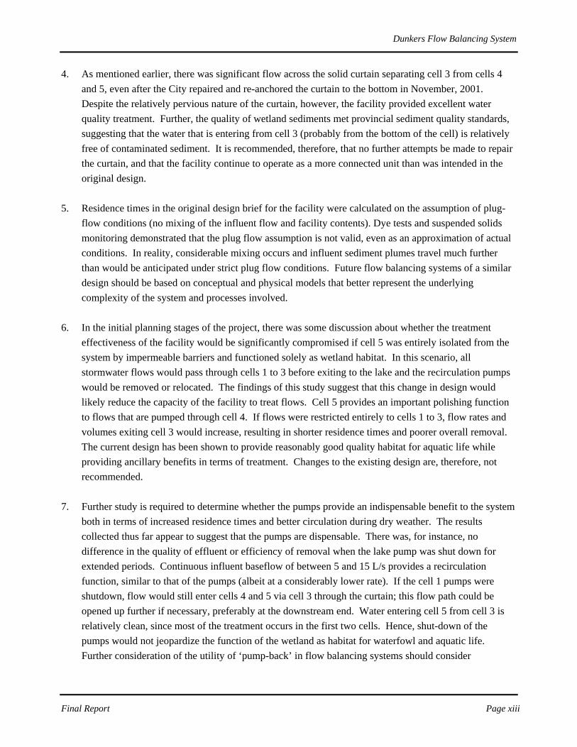
Figure 2.3: The City of Toronto Dunkers flow balancing system, indicating the location of re-circulation pumps and monitoring stations.

Dunkers Flow Balancing System
Final Report Page 8
Figure 2.4: Outlet structures at cell 3 (top) and cell 5 (bottom).

Dunkers Flow Balancing System
Final Report Page 9
Table 2.1: Storage volumes, average cell depths, pump-out times and equivalent rainfall depths for the Dunkers flow balancing system
Cell # Storage volume
(m3)
Cell area
(m2)
Maximum cell depth
(m)1
Pump-out time (hrs)2
“Retention time” (hrs)3
Rainfall depth (mm)4
1 7,900 4,720 2.6 32.9 16.5 11.6 2 9,400 5,440 2.6 39.2 52.5 13.8 3 11,200 5,510 3.2 46.7 95.5 16.5 4 2,900 1,220 3.2 12.1 12.1 4.3 5 7,800 7,060 2.0 32.5 32.5 11.5
Total 39,200 23,950 ---- ---- 104.0 5 57.8 Notes: 1. Determined from bathymetric survey. 2. Calculated as the cell storage volume divided by the pump rate, assuming only one pump is running at 4 m3/min. 3. Theoretical value based on plug-flow conditions and an event volume equal to the storage volume. 4. Equivalent to the cell storage volumes, but expressed in millimetres based on a design runoff coefficient of 0.39 for mid-sized storms. 5. Overall residence time = volume-weighted average of residence times in cells 1 to 3 plus residence times in cells 4 & 5.
The theoretical retention times shown in Table 2.1 were determined for an event volume that exactly filled the three storage cells. The theoretical values were based on plug-flow conditions and were calculated only for the pump-out operation, ignoring the fill time. In reality, the hydraulic behaviour of the system would be very complex and would include short-circuiting and dead space.
For events that discharge runoff through the cell 3 outlet structure, estimation of both the flow-through and pump-out residence times would be necessary. The former component could be estimated based on plug-flow conditions through cells 1 to 3.
In addition to providing treatment of stormwater runoff, the facility was also designed to restore the productive capacity of terrestrial and aquatic environments for fish and wildlife, an activity in keeping with the Remedial Action Plan (RAP) objective of offsetting past wetland losses in the central waterfront area wherever shelter areas exist. The cell 5 wetland was the primary means of fulfilling this goal. The extent to which the facility provides improved fish habitat in the surrounding area as compared with pre-construction degraded conditions will serve as a measure of the effectiveness of the various habitat enhancement and creation efforts.
Dunkers Flow Balancing System
Final Report Page 10
3.0 MONITORING APPROACH
This section describes the wet and dry weather monitoring program conducted in 2000, 2001 and 2002. Section 4 summarizes monitoring results for the study period.
3.1 Rainfall
Rainfall data were collected during the summer/fall and winter/spring periods using a continuous tipping bucket rain gauge, maintained by the City of Toronto, and located at the St. Augustine Seminary, south-west of Kingston and Brimley Roads (Figure 2.1). Rainfall data were also collected during the summer/fall period using similar instruments at the Dunkers facility.
3.2 Runoff
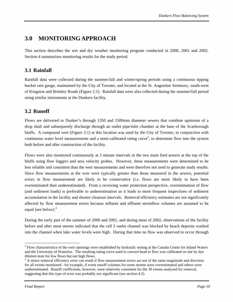
Flows are delivered to Dunker’s through 1350 and 1500mm diameter sewers that combine upstream of a drop shaft and subsequently discharge through an outlet pipe/inlet chamber at the base of the Scarborough bluffs. A compound weir (Figure 3.1) at this location was used by the City of Toronto, in conjunction with continuous water level measurements and a semi-calibrated rating curve3, to determine flow into the system both before and after construction of the facility.
Flows were also monitored continuously at 5 minute intervals in the two main feed sewers at the top of the bluffs using flow loggers and area velocity probes. However, these measurements were determined to be less reliable and consistent than the weir measurements and were therefore not used to generate study results. Since flow measurements at the weir were typically greater than those measured in the sewers, potential errors in flow measurement are likely to be conservative (i.e. flows are more likely to have been overestimated than underestimated). From a receiving water protection perspective, overestimation of flow (and sediment loads) is preferable to underestimation as it leads to more frequent inspections of sediment accumulation in the facility and shorter cleanout intervals. Removal efficiency estimates are not significantly affected by flow measurement errors because influent and effluent stormflow volumes are assumed to be equal (see below).4
During the early part of the summer of 2000 and 2001, and during most of 2002, observations of the facility before and after most storms indicated that the cell 5 outlet channel was blocked by beach deposits washed into the channel when lake water levels were high. During that time no flow was observed to occur through
3 Flow characteristics of the weir openings were established by hydraulic testing at the Canada Centre for Inland Waters and the University of Waterloo. The resulting rating curve used to convert head to flow was calibrated on site by dye dilution tests for low flows but not high flows. 4 A minor removal efficiency error can result if flow measurement errors are not of the same magnitude and direction for all events monitored - for example, if event runoff volumes for some storms were overestimated and others were underestimated. Runoff coefficients, however, were relatively consistent for the 30 events analyzed for removal, suggesting that this type of error was probably not significant (see section 4.2).
Dunkers Flow Balancing System
Final Report Page 11
the cell 5 outlet. The alternative outlet for cell 5 would be under, or through possible holes or tears in the curtains separating cell 5 from cells 3 and 4. For the purpose of data analysis, the flow out of cell 5 was assumed to be zero when the outlet channel was blocked. Ideally, both the influent and effluent flows should be measured in a monitoring study of this type. However, the design of the cell 3 and cell 5 outlets is not conducive to flow measurement. Therefore, it was assumed that the quantity of flow entering the facility was the same as the quantity of flow exiting the facility (i.e. a perfect flow balance is assumed during rain events). This was thought to be a reasonable assumption as measured baseflow influent and effluent flow rates were similar when the lake pump was shut off.
Outflow was proportioned between cell 3 and 5 based on approximations using a standard weir equation and continuous water level measurements at cell 5. These calculations revealed that, on average, roughly 25% of the total flow entering the facility during storm events exited cell 5 when the channel was clear of beach sediment. It was therefore assumed that 25% of the total flow volume entering the facility exited via cell 5, and 75% exited cell 3. The potential error in removal efficiency estimates associated with varying these relative percentages is very small because effluent concentrations at the two stations are similar (see section 3.7).
Figure 3.1: Sewer outfall structure

Dunkers Flow Balancing System
Final Report Page 12
3.3 Storage
Water level changes were measured at 5-minute intervals with Telog pressure transducers (1 psi) at the forebay, cell 2, cell 3 and at cell 5 (Figure 2.3). Water level data were combined with cell areas to determine the volume of water temporarily stored within the facility during storm events. Cell areas (m2) are based on the permanent pool elevation, 75 meters above sea level (m.a.s.l.), as estimated from a bathymetric survey of the facility in 1998.
3.4 Dye Tests
Two dye tests were conducted during the 2001 monitoring season. The first test was conducted during a wet-weather event on October 23rd to measure flow paths of stormwater through the facility. The second test, conducted on November 21st, traced the flow of the lake water being pumped into cell 3 during dry weather. Table 3.1: Fluorometer calibration
Dye Concentration
(ppb)
Fluorometer Dial
Reading
Visibility(subjective)
Scale Factor
Adjusted Fluorometer
Reading* 4760 293.9 high 1.0 9286.6 4327 287.6 high " 9086.9 3808 286.0 high " 9037.0 3173 273.3 high " 8637.5 2856 268.6 high " 8487.8 2380 246.5 moderate " 7788.8 1904 230.7 moderate " 7289.5 1269 178.5 moderate " 5641.9 952 148.5 moderate " 4693.2 476 82.2 moderate " 2596.3 428 70.0 moderate 3.16 700.0 381 66.0 moderate " 660.0 333 58.0 moderate " 580.0 286 50.0 moderate " 500.0 238 42.0 moderate " 420.0 190 35.0 moderate " 350.0 143 26.7 moderate 10.0 84.4 95.2 18.6 low " 58.9 85.7 18.0 low " 56.9 71.2 16.1 low " 50.9 66.6 14.5 low " 45.9 57.1 12.3 low " 38.9 47.6 11.1 low " 34.9 38.1 9.0 faint 31.6 9.0 28.6 7.2 faint " 7.2 19 5.0 none " 5.0
* adjusted to use the dial reading at the greatest multiplication factor as baseline

Dunkers Flow Balancing System
Final Report Page 13
3.4.1 Calibration
A series of dilutions were performed to prepare samples of the Rhodomine WT dye for analysis. The results are summarized in Table 3.1. These observations have been referenced to the lowest concentration range, at which the instrument applies a multiplier of 31.6 in order to obtain a reportable value on the read-out dial. Hence, all other observations are divided by the respective multiplier and multiplied by 31.6 to produce the adjusted reading. Visibility tests were conducted in order to relate field observations to approximate concentrations. The complete fitted curve is illustrated in Figure 3.2. Because all samples but the first bottle collected at the inlet were highly diluted, a second calibration curve was produced for the low-concentration range (Figure 3.3). The regression equation associated with this low-concentration range was used to convert fluorometer readings to dye concentrations.
0
500
1000
1500
2000
2500
3000
3500
4000
4500
5000
0 50 100 150 200 250 300 350
Voltage Reading (x31.6)
Con
cent
ratio
n (p
pb)
Figure 3.2: Complete calibration curve

Dunkers Flow Balancing System
Final Report Page 14
y = 0.0769x2 + 3.4669xR2 = 0.9911
0
10
20
30
40
50
60
70
80
90
100
0 2 4 6 8 10 12 14 16 18 20
Voltage Reading (x31.6)
Con
cent
ratio
n (p
pb)
Figure 3.3: Low-range calibration curve 3.4.2 Wet Weather Test A volume of Rhodomine WT dye (1.5 litre) was poured into the Undercliff Drive storm sewer, upstream of the drop shaft. The automatic samplers used in the regular sampling program (see figure 2.3 and section 3.5) were configured to take discrete samples at 20-minute intervals. The inlet sampler was activated by a water level change and other samplers were activated by rain gauges. The initial samples in the cells were collected after 8 hours. Samples were collected subsequently at the cell 4 inlet and the cell 3 and cell 5 outlets based on the selected sampling frequencies (1 hour for the cell 4 inlet and 2 hours for the other locations). Depth profiles of dye were determined at specific locations along the cell 1-2 pontoon and the cell 2-3 pontoon in order to detect areas where short circuiting may be occurring. Immediately following collection, samples were transported to the Ministry of the Environment laboratory for analysis. The fluorometer used for these tests was a Turner model CIO-005. The instrument includes a flow-through detection cell; a peristaltic pump was used to withdraw water from the 24 1-litre sample bottles in each sampler base, pass the sample through the instrument and return it to the sample bottle. Between samples, the tubing and detection cell were flushed with demineralized water and purged with air.

Dunkers Flow Balancing System
Final Report Page 15
3.4.3 Dry Weather Test A volume of Rhodomine WT dye (2.0 litres) was poured into the well to which lake water is pumped before being discharged through the forcemain into cell 3. Automatic discrete samplers were used for the dye test. They were positioned as in the normal monitoring program. The samplers were configured to take discrete samples at various intervals, with higher frequency sampling selected for the initial part of the test. The samplers were activated manually. The samples were collected after each 24-bottle set had been filled. As in the wet weather test, depth profiles of dye were measured at specific locations off the cell 2-3 and cell 1-2 pontoons. Once collected, samples were transported to the Ministry of the Environment laboratory and analyzed according to procedures described in section 3.4.2.
3.5 Water Quality Sampling
Samples for wet-weather water quality analysis were collected using ISCO 3700 and 6700 automated wastewater samplers at the inlet, the outlets of cells 3 and 5, the inlet and outlet of cell 4, and during 2001 and 2002, at the cell 1 and cell 2 outlets (Figure 2.3). The inlet auto-sampler was initiated by an increase in water level behind the weir; all other auto-samplers were connected to rain gauges and enabled when rainfall intensity exceeded 2 mm/hr. Start-time delays were programmed into each unit based on the observed lag between rainfall initiation and flow initiation at each of the monitoring stations.
The sampling protocol was refined over the course of the study period as new information became available and additional research questions emerged. The following sub-sections provide a summary of the water quality sampling approaches employed during each of the three monitoring seasons.
3.5.1 June to December, 2000
In 2000, all samples were time-weighted composites, collected every 5 minutes at the inlet (over a period of 120 minutes, or as long as water depths behind the weir remained 50 mm above baseflow levels), and every 10 minutes (over a maximum period of 4 hours) at cell 3, cell 5, cell 4 inlet and cell 4 outlet.
The intent of the sampling program was to attain average pollutant concentrations over a substantial portion of the event duration using unattended, automated samplers. However, during large events, influent flows may have exceeded the 120-minute sampling period and effluent flows from cell 3 and cell 5 may have exceeded the 4-hour sampling period. Also, since the influent composite samples were not flow-proportioned, substantial variation in the hydrographs and pollutographs may have resulted in errors in the estimation of average influent concentrations and pollutant mass. Potential errors in influent concentrations averaged over several events using this approach were estimated to be within ±10% (see analysis in Appendix B).

Dunkers Flow Balancing System
Final Report Page 16
Errors in the estimation of effluent concentrations using a time paced method are less than ±2% because: (i) hydrographs are not flashy; (ii) hydrographs and pollutographs do not peak simultaneously, and (iii) discrete sampling results from 2001 and 2002 monitoring indicate that concentrations are relatively uniform over the duration of most flow events (see Appendix B). At the cell 4 inlet, samples are collected from within the inlet pipe where flows are constant, either at 4 or 8 m3/min, depending on whether the second pump has been activated. A flow weighting error occurs at this station only when the second pump has been activated after the sampler has been triggered.
3.5.2 May to December 2001
Based on data analysis from the first year of monitoring, several changes to the sampling protocol were implemented at the start of the 2001 monitoring season. These changes included:
• increasing maximum sampling durations to 8 hours at all monitoring stations (20 minute sampling intervals);
• adding samplers at the downstream ends (or outlets) of cells 1 and 2, and ‘post-event’ samplers at the cell 4 inlet and cell 5 outlet; and
• flow proportioning samples for TSS based on discrete turbidity measurements and TSS-turbidity correlations.
The increase in the maximum sampling period to 8 hours more closely approximates the average duration of inflow and outflow observed in 2000. Unfortunately, time integrated composite samples collected at the inlet over an 8 hour period provide a significant underestimate of the average influent concentration because of substantial variations in pollutant concentrations and hydraulic loading, especially during the ‘first flush’. Thus inlet samples were analyzed discretely for turbidity, converted to TSS using an empirical relationship between turbidity and TSS generated from samples analyzed at each of the stations over the study period (see Figure 3.4), and then later proportioned according to flow to determine the EMC for each event. The same method was used at cells 1 and 2, but because flow was not measured at these locations, discrete turbidity samples were proportioned based on cell water level measurements.5 At the outlets to cells 3, 4 and 5, time integrated and flow proportioned composite sample results did not differ significantly, hence the 8 hour composite was taken to represent the event mean concentration for all water quality variables analyzed.
The addition of auto-samplers at cell 1 and 2 was intended to help identify where sediment and associated pollutants were settling out and how these deposition locations varied during events of different sizes and durations. Samples collected at these stations were analyzed primarily for turbidity and suspended solids.
5 Proportioning (or weighting) discrete sample concentrations based on water levels is not as accurate a representation of the EMC as proportioning discrete samples according to flow, but considerably more accurate than not proportioning at all. When pollutographs and hydrographs peak at, or close to the same time, water level proportioning typically results in an underestimate of the true EMC. This general tendency towards underestimation should be borne in mind when interpreting cell 1 and cell 2 water quality results.

Dunkers Flow Balancing System
Final Report Page 17
The intent of the ‘post event’ sampling was to characterize the change in water quality after a runoff event as water stored in cells 1 to 3 was being pumped into cells 4 and 5, and out to the lake. The additional auto-samplers were initiated with a time delay of 8 hours to correspond with the end of event sampling. Samplers were programmed to collect samples every hour at the inlet to cell 4 for a period of 24 hours, and every two hours at the cell 5 outlet for a period of 48 hours. Selection of sampling intervals was based on the expectation that the majority of suspended solids would settle over a 48 hour sampling period.
3.5.3 May to December 2002
In the 2002 season, the monitoring protocol was further improved to include discrete TSS analysis of all samples (instead of turbidity) and a second inlet sampler. The second sampler was programmed to collect samples every 10 minutes (4 hour duration) so that the ‘first flush’ into the facility could be better characterized. The sampling interval of the first sampler was maintained at 20 minutes (8 hour duration) both as a back-up to the second sampler in case of malfunction and to ensure that the entire event hydrograph was sampled.
The sampling protocol at the other monitoring stations was the same as during 2001, except that all samples for events larger than 5 mm were analyzed discretely for TSS.
Samples collected over the entire study period were preserved and submitted to the Ontario Ministry of Environment laboratory at 125 Resources Road in Etobicoke. Analysis was conducted following principles outlined in standard methods (Eaton et al., 1995) for metals, nutrients (P and N), bacteria, polynuclear aromatic hydrocarbons (PAHs), herbicides/pesticides and general chemistry (e.g. pH, alkalinity, conductivity). A portion of the discrete TSS samples analyzed in 2002 were conducted by the City of Toronto’s Dee Avenue laboratory.
3.5.4 Dry weather sampling
Grab samples were collected at the inlet, cell 3 outlet, cell 5 outlet and the lake (i.e. pumped lake water entering cell 3) during dry weather periods throughout the summer and fall of 2000 and the winter of 2001.
3.5.5 Temperature monitoring
Temperature was monitored continuously every 30 minutes at the inlet and at the cell 3 and cell 5 outlets with Ryan Temperature Monitors (RTM). In 2002, temperature was measured with the same monitors at 10 minute intervals near the outlet to cell 1 at 0.5, 1.5 and 2.5 m below the dry weather water surface. The depth integrated measurements indicated the degree of thermal stratification present in the pond during the summer, and helped to better understand flow dynamics during storm events.
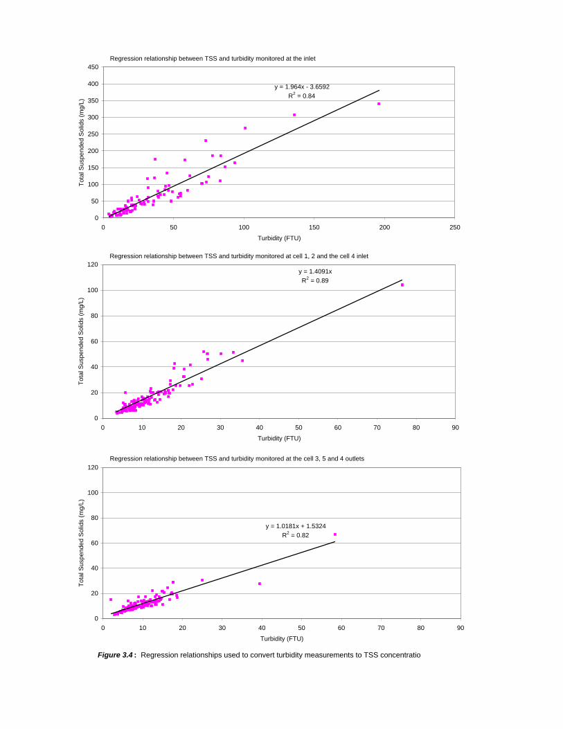
Figure 3.4 : Regression relationships used to convert turbidity measurements to TSS concentration
Regression relationship between TSS and turbidity monitored at the inlet
y = 1.964x - 3.6592R2 = 0.84
0
50
100
150
200
250
300
350
400
450
0 50 100 150 200 250
Turbidity (FTU)
Tota
l Sus
pend
ed S
olid
s (m
g/L)
Regression relationship between TSS and turbidity monitored at cell 1, 2 and the cell 4 inlet
y = 1.4091xR2 = 0.89
0
20
40
60
80
100
120
0 10 20 30 40 50 60 70 80 90
Turbidity (FTU)
Tota
l Sus
pend
ed S
olid
s (m
g/L)
Regression relationship between TSS and turbidity monitored at the cell 3, 5 and 4 outlets
y = 1.0181x + 1.5324R2 = 0.82
0
20
40
60
80
100
120
0 10 20 30 40 50 60 70 80 90
Turbidity (FTU)
Tota
l Sus
pend
ed S
olid
s (m
g/L)
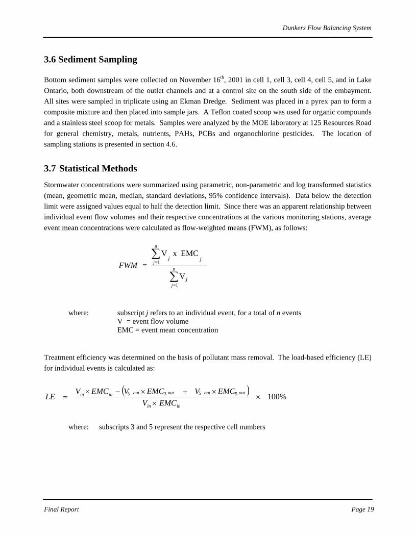
Dunkers Flow Balancing System
Final Report Page 19
3.6 Sediment Sampling
Bottom sediment samples were collected on November 16th, 2001 in cell 1, cell 3, cell 4, cell 5, and in Lake Ontario, both downstream of the outlet channels and at a control site on the south side of the embayment. All sites were sampled in triplicate using an Ekman Dredge. Sediment was placed in a pyrex pan to form a composite mixture and then placed into sample jars. A Teflon coated scoop was used for organic compounds and a stainless steel scoop for metals. Samples were analyzed by the MOE laboratory at 125 Resources Road for general chemistry, metals, nutrients, PAHs, PCBs and organochlorine pesticides. The location of sampling stations is presented in section 4.6.
3.7 Statistical Methods
Stormwater concentrations were summarized using parametric, non-parametric and log transformed statistics (mean, geometric mean, median, standard deviations, 95% confidence intervals). Data below the detection limit were assigned values equal to half the detection limit. Since there was an apparent relationship between individual event flow volumes and their respective concentrations at the various monitoring stations, average event mean concentrations were calculated as flow-weighted means (FWM), as follows:
∑
∑n
1=
1=
V
EMCx V =
j
n
j
j
jjFWM
where: subscript j refers to an individual event, for a total of n events V = event flow volume
EMC = event mean concentration
Treatment efficiency was determined on the basis of pollutant mass removal. The load-based efficiency (LE) for individual events is calculated as:
( )%1005533 ×
××+×−×
=inin
outoutoutoutinin
EMCVEMCVEMCVEMCV
LE
where: subscripts 3 and 5 represent the respective cell numbers

Dunkers Flow Balancing System
Final Report Page 20
Similarly, the long-term (or seasonal) load-based efficiency (SLE) is:
( )[ ]
[ ]%100
1
15533
××
×+×−×=
∑
∑
=
=n
iinin
n
ioutoutoutoutinin
ii
iiiiii
EMCV
EMCVEMCVEMCVSLE
where: subscript i refers to an individual event, for a total of n events
As noted above, outflow was assumed to be equal to inflow during rain events and the proportion of outflow exiting cell 3 and 5 was estimated, based on cell 5 flow measurements, to be constant at 75 and 25% of the total inflow, respectively. Since concentrations were not significantly different at the two outlets, modifying the proportion of flow exiting cell 3 and 5 resulted in relatively small changes in overall removal efficiencies. For instance, varying the proportion of flow exiting cell 5 by ±20% (i.e. from an assumed 25% downwards to 10% and upwards to 40%, and a corresponding change in cell 3 proportions) resulted in a difference in the overall (sum-of-loads) TSS removal efficiency for the same events of only ±1.7%. If events during which the cell 5 channel was blocked (i.e. when all flow exited cell 3) are included in this calculation, the error range falls from ±1.7 to ±0.6%. On this basis, a general proportioning assumption based on cell 5 flow estimates was considered to be reasonable, and efforts to establish a more precise stage-discharge curve at cell 5 were abandoned.
Dunkers Flow Balancing System
Final Report Page 21
4.0 STUDY FINDINGS
4.1 Summary of Events Monitored and System Operation
Table 4.1 summarizes the sample collection history at each monitoring station and documents changes to system function based on the operation of recirculation pumps and flow through the cell 5 outlet. Samples were collected during 64 wet-weather and 27 dry-weather events from March, 2000 to November, 2002. Among the wet-weather events monitored, not all stations were sampled, often because rainfall intensity did not exceed levels required to trigger all of the autosamplers, but also due to equipment malfunction or vandalism. Cell 1 and cell 2 stations were not monitored in 2000.
The continuous recirculation pumps (cell 3 and cell 4 feeds) were shut off for repair at various intervals over the study period. The cell 3 pump was shut down for all events monitored in 2002. Pump records indicate that the second pump at cell 1 was triggered during 11 of the storms, all of which had recorded peak inflows close to or greater than 4 m3/s. The cell 5 outlet channel was blocked by beach sediment for most of the early part of the 2000 monitoring season when lake levels were high, and over most of the 2002 season. During this period, flow through the cell 5 outlet was assumed to be zero or negligible.
When water levels in Lake Ontario are below the elevation of the two facility outlet structures, flow occurs in only one direction from the facility to the lake. As lake water levels rise above the elevation of the outlet structures, a direct two-way hydraulic connection exists between the lake and stored water in the facility. During these periods, flow continues to be discharged to the lake in response to storm runoff from the drainage catchment, but after the event, water may enter or exit the facility depending on the trend in lake levels. If, for example, lake water levels are rising over the course of a runoff event, the reduced hydraulic gradient towards the lake will help to retain the stormwater influent within the facility. Conversely, if lake water levels are declining, the increased hydraulic gradient will serve to draw new runoff water from the facility out to the lake. The lake water levels relative to the outlet structure elevations were monitored during field visits to help characterize the potential influence of lake levels on system performance (Table 4.1). Facility water level data provide in Appendix C show the trend of lake water levels during specific events.
4.2 Water Quantity
4.2.1 Rainfall and Runoff
A summary of rainfall and runoff statistics for each of the monitoring seasons is presented in Tables 4.2 to 4.4. Average rainfall over the study period ranged from 8.2 mm in 2002 to 12.3 mm in 2000. Many of the events with less than 5 mm of rain were not sampled. The 2002 monitoring season was a particularly dry year.

Inlet Cell 1 Cell 2Cell 3 outlet
Cell 4 inlet
Cell 4 outlet
Cell 5 outlet Lake ON OFF ON OFF Clear Blocked Yes No
March 15 dw C C x x x xJune 12 dw G x x x xJune 13 C x x x xJune 15 G x x x xJune 21 C x x x xJune 24 C x x x xJune 25 C x x x xJune 26 C C x x x xJune 29 C x x x xJune 29 C x x x xJuly 3 C C x x x xJuly 14 CC C C xx x x xJuly 17 C C C C xx x x xJuly 27 dw G G x x x xJuly 31 C C C C C xx x x xAugust 1 dw G G G x x x xAugust 7 C x x x xAugust 8 C C C C C xx x x xAugust 11 C x x x xAugust 23 C C C C G x x x xSeptember 2 C C C C x x x xSeptember 7 dw G G G x x x xSeptember 10 C C C C C xx x x xSeptember 11 G x x x xSeptember 14 C C C C C G x x x xSeptember 20 dw G G G G x x x xSeptember 22 C C C C C x x x xOctober 3 dw G G G G x x x xOctober 4 C C C C x x x xOctober 6 C x x x xOctober 18 dw G G G G x x x xOctober 27 C C C C C x x x xNovember 7 dw G G G G x x x xNovember 10 C C x x x x* two X's indicates second pump was triggered during rain event LegendC = Composite Sample dw = Dry weather sampleG = Grab sample
Two-way Hydraulic Connection btwn Cell
3 and the Lake
2000
Table 4.1a : Summary of sample collection, pump logs, status of the cell 5 outlet and facility-lake water connections from May 11 to November 20, 2000.
Cell 5 outletLake Ontario pumpCell 1 pumps*Monitoring Locations
Sampling Date
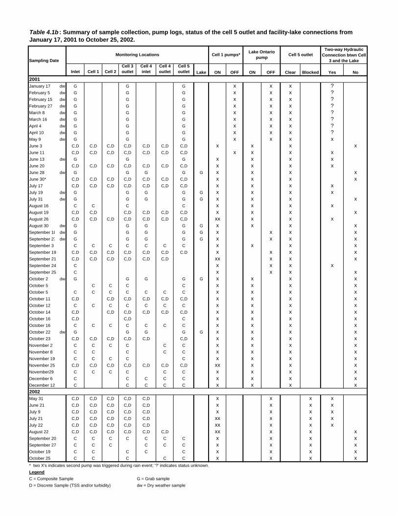
Inlet Cell 1 Cell 2Cell 3 outlet
Cell 4 inlet
Cell 4 outlet
Cell 5 outlet Lake ON OFF ON OFF Clear Blocked Yes No
January 17 dw G G G x x x ?February 5 dw G G G x x x ?February 15 dw G G G x x x ?February 27 dw G G G x x x ?March 8 dw G G G x x x ?March 16 dw G G G x x x ?April 4 dw G G G x x x ?April 10 dw G G G x x x ?May 9 dw G G G x x x xJune 3 C,D C,D C,D C,D C,D C,D C,D x x x xJune 11 C,D C,D C,D C,D C,D C,D C,D x x x xJune 13 dw G G G x x x xJune 20 C,D C,D C,D C,D C,D C,D C,D x x x xJune 28 dw G G G G G x x x xJune 30* C,D C,D C,D C,D C,D C,D C,D x x x xJuly 17 C,D C,D C,D C,D C,D C,D C,D x x x xJuly 19 dw G G G G G x x x xJuly 31 dw G G G G G x x x xAugust 16 C C C C x x x xAugust 19 C,D C,D C,D C,D C,D C,D x x x xAugust 26 C,D C,D C,D C,D C,D C,D C,D xx x x xAugust 30 dw G G G G G x x x xSeptember 18 dw G G G G G x x x xSeptember 27 dw G G G G G x x x xSeptember 3 C C C C C C C x x x xSeptember 19 C.D C,D C,D C,D C,D C,D C.D x x x xSeptember 21 C,D C,D C,D C,D C,D C,D xx x x xSeptember 24 C x x x xSeptember 25 C x x x xOctober 2 dw G G G G G x x x xOctober 5 C C C C x x x xOctober 5 C C C C C C C x x x xOctober 11 C,D C,D C,D C,D C,D C,D x x x xOctober 12 C C C C C C C x x x xOctober 14 C,D C,D C,D C,D C,D C,D x x x xOctober 16 C,D C,D C x x x xOctober 16 C C C C C C C x x x xOctober 22 dw G G G G G x x x xOctober 23 C,D C,D C,D C,D C,D C,D x x x xNovember 2 C C C C C C x x x xNovember 8 C C C C C x x x xNovember 19 C C C C C x x x xNovember 25 C,D C,D C,D C,D C,D C,D C,D xx x x xNovember29 C C C C C C x x x xDecember 6 C C C C C x x x xDecember 12 C C C C C x x x x
May 31 C,D C,D C,D C,D C,D x x x xJune 21 C,D C,D C,D C,D C,D x x x xJuly 9 C,D C,D C,D C,D C,D x x x xJuly 21 C,D C,D C,D C,D C,D xx x x xJuly 22 C,D C,D C,D C,D C,D xx x x xAugust 22 C,D C,D C,D C,D C,D C,D xx x x xSeptember 20 C C C C C C C x x x xSeptember 27 C C C C C C x x x xOctober 19 C C C C C x x x xOctober 25 C C C C C x x x x* two X's indicates second pump was triggered during rain event; '?' indicates status unknown.LegendC = Composite Sample G = Grab sampleD = Discrete Sample (TSS and/or turbidity) dw = Dry weather sample
2001
2002
Table 4.1b : Summary of sample collection, pump logs, status of the cell 5 outlet and facility-lake connections from January 17, 2001 to October 25, 2002.
Two-way Hydraulic Connection btwn Cell
3 and the LakeCell 1 pumps* Lake Ontario
pump Cell 5 outletMonitoring LocationsSampling Date

Table 4.2 : Hydrologic summary of events from June 13 to November 18, 2000
Date Time depth max. 5 min int. mean int. duration CSO(mm) (mm/5 min) (mm/hr) (hrs) Total Baseflow Runoff cell 3 cell 5 vol.
13-Jun-00 3:25 33.8 2.2 3.7 9.2 29247 444.6 28802 29247 0 1017 0.5018-Jun-00 7:40 9.2 0.8 1.7 5.3 4244 562 3682 4244 0 0 0.2521-Jun-00 2:15 7.4 1.2 0.9 8.5 3697 723 2974 3697 0 0 0.2522-Jun-00 11:40 5.6 1.8 1.1 5.3 1640 294 1346 1640 0 0 0.1524-Jun-00 17:55 1.0 0.4 3.3 0.3 349 97 252 349 0 0 0.16
24-Jun-00 b 21:05 30.6 3.0 3.1 9.8 20401 1509 18892 20401 0 219 0.3626-Jun-00 21:10 3.6 0.4 1.8 2.0 1857 444 1413 1857 0 0 0.2529-Jun-00 8:35 7.8 2.0 0.8 9.9 3095 659 2436 3095 0 27 0.183-Jul-00 2:05 3.2 0.2 0.2 12.9 1923 559 1364 1923 0 0 0.2714-Jul-00 11:00 21.6 4.6 2.0 10.6 19342 629 18713 19342 0 659 0.5115-Jul-00 20:40 5.5 2.0 7.3 0.8 4115 346 3769 4115 0 0 0.4316-Jul-00 7:25 12.2 3.8 1.2 10.1 6550 542 6008 6550 0 362 0.2917-Jul-00 19:20 31.2 4.2 23.5 1.3 29148 2283 26865 29148 0 980 0.5030-Jul-00 22:40 30.2 7.2 8.8 3.4 18987 880 18107 14240 4747 1126 0.357-Aug-00 4:00 3.1 1.3 2.2 1.4 965 208 757 965 0 0 0.158-Aug-00 15:20 19.4 4.0 2.8 7.0 11993 659 11334 11993 0 413 0.3411-Aug-00 3:10 7.2 2.4 9.6 0.8 2110 230 1881 2110 0 0 0.1623-Aug-00 1:05 23.2 2.2 3.1 7.5 12166 475 11691 9125 3042 280 0.292-Sep-00 14:25 5.5 0.7 0.8 6.9 2551 394 2157 2551 0 0 0.2510-Sep-00 18:15 18.0 5.4 6.5 2.8 10555 175 10380 7916 2639 685 0.3411-Sep-00 0:25 11.0 3.0 1.7 6.6 7093 543 6550 5320 1773 0 0.3714-Sep-00 12:45 22.0 2.0 2.9 7.5 10263 655 9608 7697 2566 0 0.2722-Sep-00 22:40 18.6 1.0 1.1 17.0 10154 487 9667 7616 2539 45 0.3023-Sep-00 18:10 5.8 5.4 23.2 0.3 3346 403 2943 2510 837 18 0.304-Oct-00 4:50 6.6 0.8 1.2 5.4 2500 250 2250 2500 0 0 0.215-Oct-00 16:50 2.4 0.2 0.4 5.5 1819 486 1333 1819 0 0 0.356-Oct-00 17:30 3.2 0.2 0.2 17.3 168 84 84 168 0 0 0.0224-Oct-00 12:05 4.2 0.6 0.4 10.6 1346 112 1234 1346 0 0 0.1827-Oct-00 8:55 2.6 1.2 1.0 2.6 1034 104 930 1034 0 0 0.2210-Nov-00 3:20 13.8 0.6 1.6 8.8 8194 410 7784 6146 2049 0 0.35Averages
all storms 12.3 2.2 3.9 6.6 7695 522 7174 7022 673 194 0.29storms with rain > 5mm 15.2 2.6 4.7 6.8 9709 614 9096 8832 878 254 0.32
2. Catchment area with and without combined sewer overflow is 171 and 159.1 ha, respectively.
Runoff Coeff.2
Flow Volume (m3)RainInlet Outlets1
1. When the cell 5 outlet channel was clear of sediment, outflow through cell 3 and 5 was assumed to be 75 and 25% of total inflow, respectively.

Table 4.3 : Hydrologic summary of events from January 30 to November 30, 2001
Date Time depth max. 5 min int. mean int. duration CSO(mm) (mm/5 min) (mm/hr) (hrs) Total Baseflow Runoff cell 3 cell 5 vol.
30-Jan-01 4:40 5.6 0.2 0.8 7.3 3460 7 3453 2595 865 15 0.368-Feb-01 23:10 24.6 1.2 1.3 18.7 31884 1322 30562 23913 7971 1360 0.73
25-Feb-01 0:50 18.4 1.6 4.3 4.3 17524 1078 16446 13143 4381 0 0.5613-Mar-01 5:25 8.4 0.8 1.4 6.0 6242 651 5591 4682 1561 50 0.397-Apr-01 8:10 1.6 0.2 0.8 1.9 739 124 615 554 185 0 0.24
7-Apr-01 b 21:20 8.2 3.2 4.3 1.9 5146 452 4695 3860 1287 92 0.339-Apr-01 11:15 6.6 1.0 1.7 3.8 7671 460 7211 5753 1918 0 0.6912-Apr-01 3:25 2.6 0.8 0.4 5.8 1728 333 1395 1296 432 0 0.3421-May-01 12:25 7.4 1.0 3.2 2.3 3399 189 3210 2549 850 0 0.2721-May-01 23:05 9.4 0.8 3.1 3.0 5959 443 5516 4469 1490 0 0.37
22-May-01 b 16:35 21.4 1.4 3.2 6.6 14981 1006 13975 11236 3745 351 0.3827-May-01 12:50 16.4 2.0 5.7 2.9 8015 370 7645 6011 2004 0 0.2928-May-01 4:25 0.8 2.2 0.1 7.5 1169 749 420 877 292 0 0.331-Jun-01 10:35 6.4 0.8 0.7 9.8 3326 519 2807 2495 832 0 0.283-Jun-01 0:45 5.2 1.4 4.3 1.2 2378 206 2172 1784 595 0 0.2611-Jun-01 0:45 18.2 1.7 2.0 8.9 8555 590 7965 6416 2139 0 0.2820-Jun-01 2:05 4.1 1.3 0.8 5.3 1344 239 1105 1008 336 0 0.1722-Jun-01 1:25 2.6 0.4 0.4 6.2 1156 389 767 867 289 0 0.1930-Jun-01 20:10 5.6 2.2 7.0 0.8 2041 242 1799 1531 510 0 0.201-Jul-01 9:00 10.8 5.8 36.0 0.3 5072 254 4818 3804 1268 345 0.2617-Jul-01 0:15 12.4 1.6 1.7 7.5 4646 514 4132 3485 1162 0 0.2116-Aug-01 17:50 5.2 0.6 0.5 11.4 2682 435 2247 2012 671 0 0.2719-Aug-01 7:05 9.2 0.6 1.5 6.1 6035 663 5372 4526 1509 0 0.3726-Aug-01 13:40 11.2 5.0 2.9 3.8 5202 419 4784 3902 1301 248 0.253-Sep-01 21:55 4.0 1.2 0.6 6.8 2379 467 1912 1784 595 0 0.28
19-Sep-01 14:30 24.4 1.8 2.1 11.5 15520 1010 14510 11640 3880 0 0.3721-Sep-01 13:40 22.4 2.6 2.6 8.6 14030 724 13306 10523 3508 279 0.3525-Sep-01 6:15 2.2 0.4 0.9 2.4 1887 691 1196 1415 472 0 0.3426-Sep-01 1:20 2.0 0.2 0.9 2.3 1216 399 817 912 304 0 0.26
26-Sep-01 b 19:10 2.0 0.2 0.5 4.1 768 297 471 576 192 0 0.154-Oct-01 22:15 7.0 0.6 1.0 7.3 2355 286 2069 1766 589 0 0.195-Oct-01 7:10 38.8 0.6 5.3 7.3 21407 1600 19807 16055 5352 0 0.32
11-Oct-01 17:15 19.2 0.6 1.2 15.9 9878 675 9203 7409 2470 0 0.3014-Oct-01 9:50 7.6 1.2 0.8 10.0 4722 859 3863 3542 1181 0 0.3216-Oct-01 5:30 11.4 0.4 0.9 12.2 7608 984 6624 5706 1902 0 0.3723-Oct-01 11:40 7.1 1.8 5.1 1.4 3255 338 2917 2441 814 0 0.262-Nov-01 7:25 10.0 0.6 2.0 5.0 6145 437 5708 4609 1536 0 0.3625-Nov-01 2:40 25.2 4.5 4.5 5.6 15000 301 14699 11250 3750 452 0.3429-Nov-01 1:35 11.4 0.4 0.8 14.4 6830 277 6553 5123 1708 0 0.3629-Nov-01 20:50 16.0 0.4 1.2 13.3 10409 1943 8466 7807 2602 0 0.33
Averagesall storms 10.8 1.4 3.0 6.5 6844 573 6271 5133 1711 80 0.32storms with rain > 5mm 13.0 1.6 3.6 7.1 8242 616 7626 6182 2061 100 0.34
2. Catchment area with and without combined sewer overflow is 171 and 159 ha, respectively.
Runoff Coef.2
Rain Flow Volume (m3)Inlet Outlets1
1. Outflow through cell 3 and 5 was assumed to be 75 and 25% of total inflow, respectively.

Table 4.4: Hydrologic summary of events from February 20 to November 5, 2002
Date Time depth max. 5 min int. mean int. duration CSO(mm) (mm/5 min) (mm/hr) (hrs) Total Baseflow Runoff Cell 3 Cell 5 vol.
20-Feb-02 6:10 13.2 0.6 1.1 11.8 21242 2980 18262 21242 0 10 0.813-Mar-02 20:05 14.0 0.8 2.1 6.6 18279 885 17394 18279 0 52 0.7312-Apr-02 13:05 22.0 2.8 2.2 10.2 11954 894 11060 11954 0 302 0.2913-Apr-02 12:20 6.0 0.6 1.5 3.9 6578 2683 3895 6578 0 0 0.4128-Apr-02 3:00 11.4 0.4 0.7 17.0 12176 2075 10101 12176 0 4 0.522-May-02 3:45 8.2 1.0 2.6 3.1 8364 831 7533 8364 0 178 0.54
2-May-02 b 21:30 3.6 2.4 1.4 2.5 1767 638 1129 1767 0 0 0.2013-May-02 15:10 8.0 0.4 1.1 7.0 8646 2365 6281 8646 0 0 0.4916-May-02 8:10 2.4 0.4 1.4 1.8 1303 428 875 1303 0 0 0.23
16-May-02 b 17:25 16.8 0.8 2.9 5.8 12277 2592 9685 12277 0 40 0.3431-May-02 5:00 6.8 1.5 3.8 1.8 3577 421 3156 3577 0 0 0.2911-Jun-02 21:45 3.0 0.6 2.3 1.3 1040 184 856 1040 0 0 0.1812-Jun-02 3:35 3.0 0.8 1.2 2.6 1480 279 1201 1480 0 0 0.2514-Jun-02 10:25 4.4 1.2 1.2 3.8 2685 360 2325 2685 0 0 0.3315-Jun-02 9:50 1.4 0.4 2.8 0.5 505 170 335 505 0 0 0.15
15-Jun-02 b 17:20 6.2 0.8 1.3 4.6 2643 343 2300 2643 0 0 0.2316-Jun-02 5:05 2.4 0.4 0.8 3.1 1429 277 1152 1429 0 0 0.30
16-Jun-02 b 12:15 3.6 1.6 9.0 0.4 1427 284 1143 1427 0 0 0.2021-Jun-02 14:55 12.7 5.1 3.2 4.0 5704 494 5210 5704 0 0 0.2626-Jun-02 20:20 2.0 0.4 1.8 1.1 661 153 508 661 0 0 0.169-Jul-01 3:30 5.0 1.5 1.8 2.8 2157 375 1782 2157 0 0 0.2218-Jul-02 16:25 6.2 1.0 5.6 1.1 3592 351 3241 3592 0 0 0.3321-Jul-02 22:40 25.7 4.3 10.7 2.4 12338 466 11872 12338 0 364 0.2722-Jul-02 14:45 23.3 5.7 6.1 3.8 12603 443 12160 12603 0 1771 0.3123-Jul-02 1:15 3.4 1.0 0.8 4.3 2018 514 1504 2018 0 0 0.2828-Jul-02 9:25 3.8 0.4 3.2 1.2 1883 297 1586 1883 0 0 0.2629-Jul-02 21:00 2.0 0.4 2.9 0.7 1133 261 872 1133 0 0 0.2722-Aug-02 9:50 7.5 3.5 4.7 1.6 3850 440 3410 3850 0 58 0.2714-Sep-02 20:55 15.7 3.2 1.9 8.2 10525 645 9880 10525 0 0 0.4015-Sep-02 18:35 2.0 0.2 1.1 1.8 1008 323 685 1008 0 0 0.2220-Sep-02 6:20 3.0 0.8 2.7 1.1 1249 248 1002 937 312 0 0.2121-Sep-02 3:45 1.2 0.2 0.5 2.3 553 234 319 415 138 0 0.1727-Sep-02 7:45 36.8 1.2 3.8 9.6 23397 713 22684 17548 5849 115 0.362-Oct-02 2:00 2.2 0.8 0.6 3.4 1481 367 1114 1111 370 0 0.324-Oct-02 22:00 4.2 0.8 2.3 1.8 2263 297 1966 1697 566 21 0.2716-Oct-02 12:55 3.4 0.2 0.5 6.5 1101 344 757 826 275 0 0.1418-Oct-02 20:15 10.8 0.6 0.7 15.7 5013 573 4440 3760 1253 0 0.2622-Oct-02 4:50 5.4 0.4 0.8 7.1 3203 722 2481 2402 801 0 0.2925-Oct-02 20:30 8.8 0.4 1.4 6.5 4813 310 4503 3610 1203 0 0.325-Nov-02 21:00 4.8 0.2 0.7 6.8 2338 175 2163 1754 585 0 0.28Averages
all storms 8.2 1.2 2.4 4.5 5506 686 4821 5223 191 73 0.31storms with rain > 5mm 13.3 1.8 2.9 6.6 9539 1061 8477 9083 455.3 145 0.39
2. Catchment area with and without combined sewer overflow is 171 and 159.1 ha, respectively.
Runoff Coeff.2
Rain Flow Volume (m3)Inlet Outlets1
1. Inflow and outflow volumes were assumed to be equal during storm events. The cell 5 outlet channel was blocked with beach sediment for the entire 2002 monitoring season.

Dunkers Flow Balancing System
Final Report Page 27
Influent baseflow was continuous throughout the monitoring period with typical dry weather summer values between 5 and 10 L/s. Combined sewer overflows occurred during 32 of the 110 events monitored, but represented only 1.6% of total runoff volumes. Average runoff coefficients were relatively consistent over the three monitoring seasons ranging from 0.29 to 0.32. Runoff coefficients were particularly high during the winter when rain combined with snow melt can result in high runoff values. Significant departures in individual runoff coefficients from seasonal averages during non-winter periods (e.g. Oct 16, 2002; July 17, 2000) reflect a combination of errors in rainfall and flow measurements, differences in antecedent moisture conditions (especially in the spring) and the statistical tendency for larger events to generate proportionately more runoff than smaller events.
Event based water level changes at the inlet chamber and cells 1, 2, 3 and 5 are presented in Figure 4.1. The time delay between level increases at the inlet chamber and cell 3 averaged less than 10 minutes during rain events. As expected, level fluctuations in cells 2 and 3 were almost identical. Cell 1 changes were also similar, but, during high flow, the permeable curtain immediately upstream of the measurement point tended to produce erratic water level fluctuations (i.e. waves) when flow input exceeded the hydraulic capacity of the curtain to conduct water. The time required for water levels to return to baseflow levels was similar at cells 1, 2 and 3, averaging approximately 11 hours (Figure 4.1).
Throughout the study period, there was little difference in water level fluctuations between cell 4/5 and cells 1 to 3 during runoff events (Fig. 4.1).1 If the pump station were the only source of flow into cell 4/5, a greater differential in water levels would have been expected. Flow around or under the curtain - and possibly flow through holes in the curtain created by beavers - were apparently allowing the runoff to enter cells 4 and 5 from cell 3. Raising the cell 3-4 curtain to eliminate obvious gaps near the banks in September 2000, and repair and re-anchoring of the curtain in late 2001 had little effect on creating even short-term water level differentials between cell 5 and cells 1 to 3 during storm events.2
Figure 4.2 shows flow hydrographs at the inlet, cell 5 outlet and at the curtain separating cell 3 and 4 for events on August 23rd and September 14th, 2000. Flow volumes through the curtain represent the product of incremental storage volumes in cell 4 and 5 (area = 8280 m2) and estimated flow from cell 5 to the lake. Short-term fluctuations in the curve resulting from small variations ("1 to 2 mm) in level measurements (perhaps due to wave action) were reduced by pooling each set of three data points (5 minutes each) into 15 minute moving averages. The graphs indicate that cell 5 provided significant peak flow attenuation. Note that the water elevations and flows are presented relative to the dry-weather baseline; baseflow is not shown.
1 A previous interim report indicated minor differences in peak water levels between cell 3 and cell 5 in August and September 2000. These differences were later determined to have been caused by the location of the sensor in the narrow cell 5 channel where some throttling of flow occurs. In 2001 and 2002 the sensor was relocated to the open water portion of cell 5. 2 Note that the solid curtain was not intended to be completely impervious to flow. However, there was an expectation that the solid curtain would prevent flow from entering cells 4 and 5 during large runoff events, creating an observable difference in surface water fluctuations on short time scales.
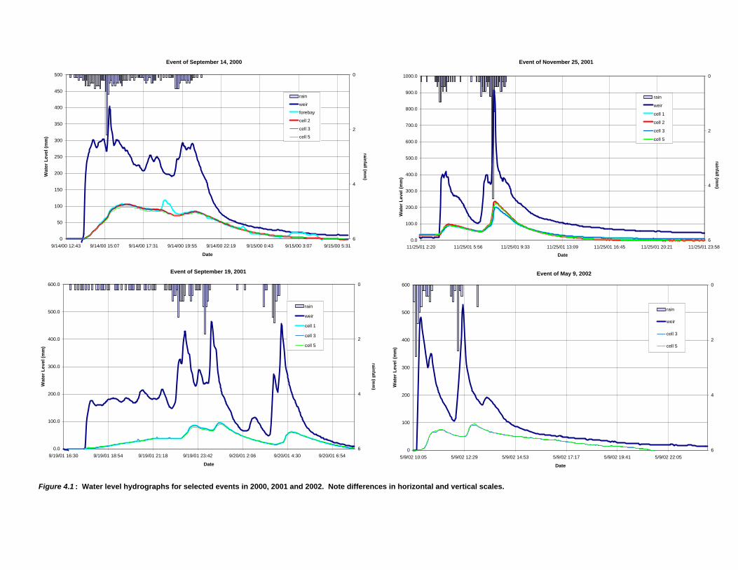
Figure 4.1 : Water level hydrographs for selected events in 2000, 2001 and 2002. Note differences in horizontal and vertical scales.
Event of November 25, 2001
0.0
100.0
200.0
300.0
400.0
500.0
600.0
700.0
800.0
900.0
1000.0
11/25/01 2:20 11/25/01 5:56 11/25/01 9:33 11/25/01 13:09 11/25/01 16:45 11/25/01 20:21 11/25/01 23:58
Date
Wat
er L
evel
(mm
)
0
2
4
6
rainfall (mm
)
rain
weir
cell 1
cell 2
cell 3
cell 5
Event of September 14, 2000
0
50
100
150
200
250
300
350
400
450
500
9/14/00 12:43 9/14/00 15:07 9/14/00 17:31 9/14/00 19:55 9/14/00 22:19 9/15/00 0:43 9/15/00 3:07 9/15/00 5:31
Date
Wat
er L
evel
(mm
)
0
2
4
6
rainfall (mm
)
rain
weir
forebay
cell 2
cell 3
cell 5
Event of September 19, 2001
0.0
100.0
200.0
300.0
400.0
500.0
600.0
9/19/01 16:30 9/19/01 18:54 9/19/01 21:18 9/19/01 23:42 9/20/01 2:06 9/20/01 4:30 9/20/01 6:54
Date
Wat
er L
evel
(mm
)
0
2
4
6
rainfall (mm
)
rain
weir
cell 1
cell 3
cell 5
Event of May 9, 2002
0
100
200
300
400
500
600
5/9/02 10:05 5/9/02 12:29 5/9/02 14:53 5/9/02 17:17 5/9/02 19:41 5/9/02 22:05
Date
Wat
er L
evel
(mm
)
0
2
4
6
()
rain
weir
cell 3
cell 5

Dunkers Flow Balancing System
Final Report Page 29
August 23, 2000
0
500
1000
1500
2000
2500
3000
3500
4000
1:24 2:36 3:48 5:00 6:12 7:24 8:36 9:48 11:00
Flow
(L/s
)
0
2
4
6
8
10
Rainfall (m
m)
rainfall
Inlet
cell 3 to cell 4
cell 5 to Lake
Sept 14, 2000
0
100
200
300
400
500
600
700
800
12:00 13:12 14:24 15:36 16:48 18:00 19:12 20:24 21:36 22:48
Flow
(L/s
)
0
2
4
6
8
10
Rainfall (mm
)
rainfall
Inlet (calibrated weir)
cell 3 to cell 4
cell 5 to Lake
Figure 4.2: Hyetographs and hydrographs at the inlet, cell 5 outlet and at the curtain separating cells 3 and 4 for events on August 23 and September 14, 2000.
(Flow through the curtain was calculated from cell 5 outflow and incremental storage changes in cells 4 & 5.)
Dunkers Flow Balancing System
Final Report Page 30
4.3 Dye Tests Two dye tests were conducted in 2001: one during wet weather and one during dry weather. The purpose of the wet weather test was to delineate flow paths of stormwater through the facility and identify dead zones (if any) or areas of short circuiting. The dry weather test aimed to trace the path of lake water being pumped into cell 3 in order to characterize the nature and efficiency of the post-event recirculation process. 4.3.1 Wet Weather Dye Test On October 23rd, a rain event began at 12:10 (daylight savings time) but the initial precipitation was minor. The wind was moderate and from the west. The dye was applied to the storm sewer upstream of the dropshaft at 12:49 when a more intense period of rain began. The total rainfall was 7.1 mm, of which 6.7 mm fell in less than one hour. The rain event ended at 13:30. Figure 4.3 shows the hyetograph, inlet hydrograph, facility water levels and dye concentrations during the initial period of runoff. The location of sampler intakes is the same as that for the regular monitoring program (see Figure 2.3). Over this period, dye was detected at all stations except the cell 3 and cell 5 outlets. Dye did reach these stations, but only after baseflow had been re-established, as discussed below. The sampler information was supplemented with detailed visual observations. These visual observations and a chronology of the test are summarized in Table 4.5. Figures 4.4 and 4.5 show photographs taken during the test. Figure 4.6 illustrates the progression of the dye through the system based on visual observations (Table 4.5) and initial detection in the samplers (Figure 4.3). The dye wave-front lines in this figure were obtained by interpolation. The lines representing approximately the first two hours are based mostly on visual observations and are reasonably accurate. Later wave-front line shapes are estimated, with the time scale based on sampler data. Note that the wavefront line interval varies in this Figure. During the initial part of the event, the interval is 5 minutes; it increases to 10 minutes as the event slows and subsequently transitions to 1 hour after the event.

Figure 4.3 : Hydrographs, hyetographs and dye concentrations during the initial period of runoff. Note that the cell 4 inlet sampler malfunctioned and was initiated manually 3 hours after the start of runoff.
0
0.5
1
1.5
2
2.5
12:15 12:55 13:35 14:15 14:55 15:35 16:15 16:55 17:35 18:15 18:55
Rai
n (m
m)
0
250
500
750
1000
1250
1500
1750
12:15 12:55 13:35 14:15 14:55 15:35 16:15 16:55 17:35 18:15 18:55
FLow
(L/s
)
020406080100120140160180
Wat
er L
evel
(mm
)
Inlet Flow
Facility Water Level
0
20
40
60
80
100
120
12:15 12:55 13:35 14:15 14:55 15:35 16:15 16:55 17:35 18:15 18:55
Dye
Con
cent
ratio
n (p
pb) Cell 1 Cell 2
Cell 4 in Cell 4 out
Cell 3 cell 5
Total Precipitation = 7.1 mm
Total Inflow Volume = 3,300 m3
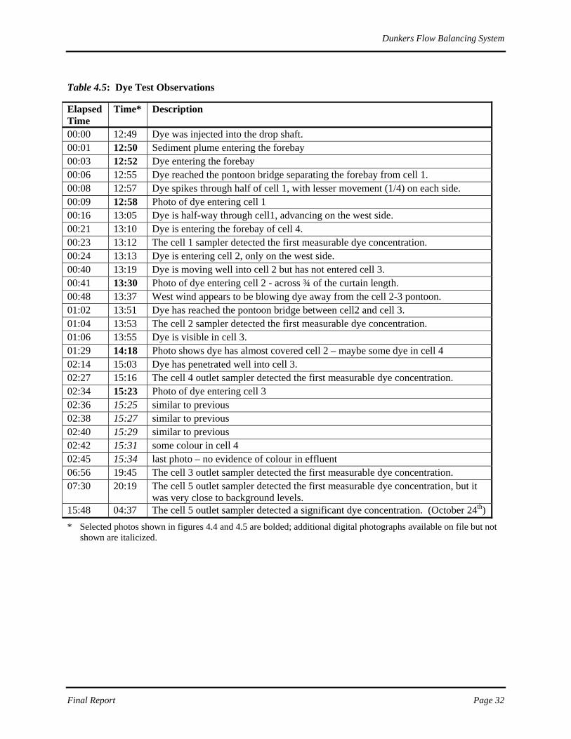
Dunkers Flow Balancing System
Final Report Page 32
Table 4.5: Dye Test Observations
Elapsed Time
Time* Description
00:00 12:49 Dye was injected into the drop shaft. 00:01 12:50 Sediment plume entering the forebay 00:03 12:52 Dye entering the forebay 00:06 12:55 Dye reached the pontoon bridge separating the forebay from cell 1. 00:08 12:57 Dye spikes through half of cell 1, with lesser movement (1/4) on each side. 00:09 12:58 Photo of dye entering cell 1 00:16 13:05 Dye is half-way through cell1, advancing on the west side. 00:21 13:10 Dye is entering the forebay of cell 4. 00:23 13:12 The cell 1 sampler detected the first measurable dye concentration. 00:24 13:13 Dye is entering cell 2, only on the west side. 00:40 13:19 Dye is moving well into cell 2 but has not entered cell 3. 00:41 13:30 Photo of dye entering cell 2 - across ¾ of the curtain length. 00:48 13:37 West wind appears to be blowing dye away from the cell 2-3 pontoon. 01:02 13:51 Dye has reached the pontoon bridge between cell2 and cell 3. 01:04 13:53 The cell 2 sampler detected the first measurable dye concentration. 01:06 13:55 Dye is visible in cell 3. 01:29 14:18 Photo shows dye has almost covered cell 2 – maybe some dye in cell 4 02:14 15:03 Dye has penetrated well into cell 3. 02:27 15:16 The cell 4 outlet sampler detected the first measurable dye concentration. 02:34 15:23 Photo of dye entering cell 3 02:36 15:25 similar to previous 02:38 15:27 similar to previous 02:40 15:29 similar to previous 02:42 15:31 some colour in cell 4 02:45 15:34 last photo – no evidence of colour in effluent 06:56 19:45 The cell 3 outlet sampler detected the first measurable dye concentration. 07:30 20:19 The cell 5 outlet sampler detected the first measurable dye concentration, but it
was very close to background levels. 15:48 04:37 The cell 5 outlet sampler detected a significant dye concentration. (October 24th) * Selected photos shown in figures 4.4 and 4.5 are bolded; additional digital photographs available on file but not
shown are italicized.
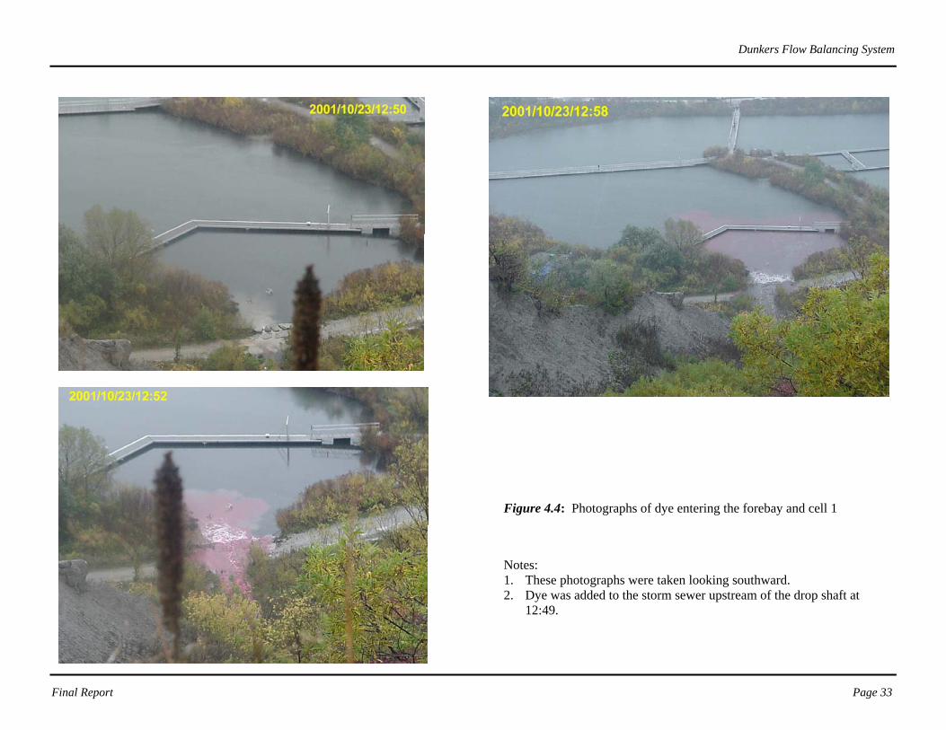
Dunkers Flow Balancing System
Final Report Page 33
Figure 4.4: Photographs of dye entering the forebay and cell 1 Notes: 1. These photographs were taken looking southward. 2. Dye was added to the storm sewer upstream of the drop shaft at
12:49.

Dunkers Flow Balancing System
Final Report Page 34
Figure 4.5: Photographs of Dye Entering Cells 2 and 3 Notes: 1. The sampler on the cell 1 side of the cell 1-2 curtain first detected the
dye at 13:12. 2. The sampler on the cell 2 side of the cell 2-3 curtain first detected the
dye at 13:53. 3. Subsequent photographs provide little additional information because
of the overcast conditions, the dilution of the dye and the slow progression of the dye beyond this time.
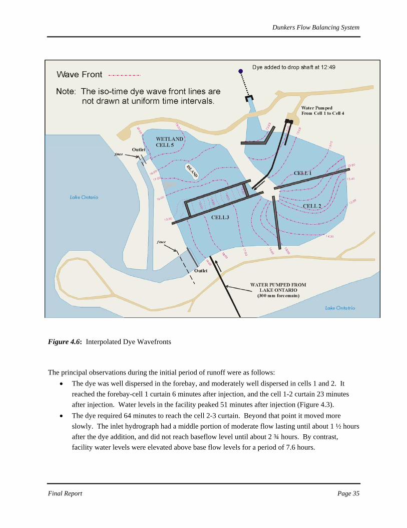
Dunkers Flow Balancing System
Final Report Page 35
Figure 4.6: Interpolated Dye Wavefronts The principal observations during the initial period of runoff were as follows:
• The dye was well dispersed in the forebay, and moderately well dispersed in cells 1 and 2. It reached the forebay-cell 1 curtain 6 minutes after injection, and the cell 1-2 curtain 23 minutes after injection. Water levels in the facility peaked 51 minutes after injection (Figure 4.3).
• The dye required 64 minutes to reach the cell 2-3 curtain. Beyond that point it moved more slowly. The inlet hydrograph had a middle portion of moderate flow lasting until about 1 ½ hours after the dye addition, and did not reach baseflow level until about 2 ¾ hours. By contrast, facility water levels were elevated above base flow levels for a period of 7.6 hours.

Dunkers Flow Balancing System
Final Report Page 36
• The dye dispersion pattern at the surface for the initial hour suggested that the desired horizontal plug-flow conditions of the storage facility were achieved, within the practical constraints of the system geometry.
• Visual observations at the surface indicated that dye reached the cell 1 pump station intake location in about 10 minutes, but was visually detected at the forcemain headwall in the cell 4 forebay only after 21 minutes. Since the intake is located near the bottom of cell 1, the 11 minute difference suggests that dye was moving more quickly across the surface than at the bottom of the pond (i.e. vertical plug flow conditions were achieved only after a delay). Dye was detected at the cell 1-2 curtain two minutes after detection at the cell 4 headwall.
• The previous observation is also confirmed through simple volume calculations. The total volume of inflow during the event was approximately 3300 m3. If plug flow conditions prevailed, the water would enter the facility, and travel only as far as would be required to displace an equivalent volume of water. Since the volume of cell 1 is 7900 m3, one would expect, under strict plug flow conditions, that the dye would progress through only half of the cell. This was, of course, not the case, indicating that a plug flow assumption drastically underestimates the distance that new influent runoff will travel in wet pond type facilities.
• The dye required a little more than 2 hours to move through cell 4 and be detected at the cell 4 outlet sampler. Plug flow in this cell (volume = 2,900 m3) at a pumping rate of 4 m3/min would require approximately 12 hours to move from one end to the other. With two pumps running, the theoretical residence time would be 6 hours; however, the second pump was not triggered during this event. There are two possible explanations for the reduced residence time in cell 4: (i) flow through cell 4 was not uniform in cross-section (i.e. flow moved more quickly across the surface where the sampler intake was located), or (ii) flow was entering cell 4 from cell 3 through holes in or beneath the curtain causing the dye to move at a faster rate than it otherwise would have. This is not to suggest that dye was entering cell 4 from cell 3 (the timing of dye observations in cell 3 would not support that interpretation), but rather that flow into cell 4 caused by a head differential across the leaky curtain pushed the dye through the cell at a rate faster than could be explained by pump discharge alone.
• The dye required 5.9 hours to cross cell 3 (6.5 hours after dye was added to the storm sewer). After dye entered cell 3 from cell 2, facility water levels were receeding (Figure 4.3), causing the dye to move more slowly than at the beginning of the event. The dye was detected at the cell 3 outlet only 25 minutes before facility water levels returned to pre-event baseflow levels. Flow through the cell would have been opposed by the pumped lake water that moves in the opposite direction, although the actual two-directional flow pattern, and the pattern of dye movement, would depend on many factors including wind and water temperature.
• The dye required approximately 5 hours to cross cell 5 (7.5 hours after dye was added to the sewer). However the initial fluorometer readings were so close to background levels that it was uncertain whether dye was indeed present. Significant dye concentration occurred at the cell 5 outlet 13.3 hours after detection at the cell 4 outlet (15.9 hours after dye was added to the sewer). Dye transport would have been caused by diffusion and the pumped flow rate (plus or minus any leakage through or under the cell 3-4-5 curtain). The fact that the dye concentration increased

Dunkers Flow Balancing System
Final Report Page 37
significantly about 8.5 hours after first detection (13.5 hour residence time) may have been due to additional precipitation. There was some rain on the morning of the 24th, more during the early hours of the 25th and traces of precipitation on the 26th.
The dye tracer fluorometer results for the event and post event period are presented in Figure 4.7. Post event sampling was conducted at the two facility outlets and at the cell 4 inlet. Sampling was not continued for a sufficient period of time to provide a complete dye tracer curve. A discussion of the results follows:
• The event on October 23rd was followed by three other smaller rain events: 2 mm from 10:40 to 11:40 on October 24th, 4.8 mm from 0:15 to 3:15 on October 25th, and 0.8 mm from 14:50 to 15:15 on October 26th (Figure 4.7).
• At approximately 8:10 on the 24th of October, water levels in the facility started to rise independently of rainfall within the catchment. These levels continued to rise until midnight on the 29th (see Appendix C) and are attributed to rising lake levels. Once the lake level rises above the base of the cell 3 and 5 outlet structures, water level fluctuations in the facility parallel those of the lake.
• The concentration peaks at the cell 1, cell 2 and cell 3 sampling locations follow a progression as would be expected.
• The second peak in the cell 3 outlet curve corresponds with the decline in water level after the small event on October 24th. As the water level declines, dye exits the facility. When the direction of flow reversed (beginning at roughly 20:00, October 24th) lake water starts to flow into the facility, and cell 3 concentrations begin to decline.
• The cell 4 influent curve reflects the fact that the stormwater was being held in cell 1 and transferred to cell 4 by pump. The rainfall event on the morning of the 24th also seems to have influenced the curve shape by causing a second peak.
• The weak concentration in the cell 4 outlet curve suggests dilution from water entering cell 3 through the cell 3-4 curtain (see Figure 4.7). If cell 4 had been isolated, the conservative dye should have appeared almost as concentrated in the effluent as it was in the influent, but with the time of appearance shifted by an amount equal to the residence time in cell 4.
• On October 25th, when 4.8 mm of rain fell between 00:15 and 03:15, the cell 4 influent dye concentration again appears to have responded to the residual dye in the forebay and cell 1. Only the cell 5 outlet concentration was being monitored when a small rainfall event occurred on the 26th.
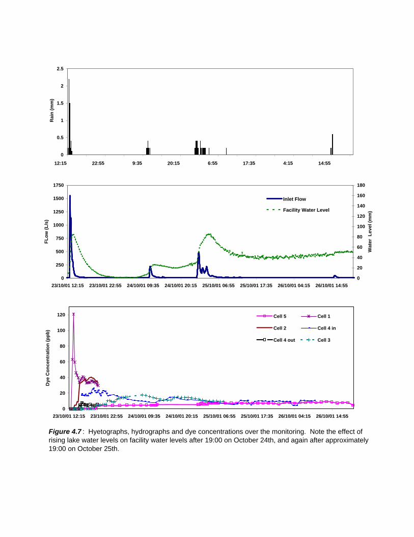
Figure 4.7 : Hyetographs, hydrographs and dye concentrations over the monitoring. Note the effect of rising lake water levels on facility water levels after 19:00 on October 24th, and again after approximately 19:00 on October 25th.
0
0.5
1
1.5
2
2.5
12:15 22:55 9:35 20:15 6:55 17:35 4:15 14:55
Rai
n (m
m)
0
20
40
60
80
100
120
23/10/01 12:15 23/10/01 22:55 24/10/01 09:35 24/10/01 20:15 25/10/01 06:55 25/10/01 17:35 26/10/01 04:15 26/10/01 14:55
Dye
Con
cent
ratio
n (p
pb)
Cell 5 Cell 1
Cell 2 Cell 4 in
Cell 4 out Cell 3
0
250
500
750
1000
1250
1500
1750
23/10/01 12:15 23/10/01 22:55 24/10/01 09:35 24/10/01 20:15 25/10/01 06:55 25/10/01 17:35 26/10/01 04:15 26/10/01 14:55
FLow
(L/s
)
0
20
40
60
80
100
120
140
160
180
Wat
er L
evel
(mm
)
Inlet Flow
Facility Water Level
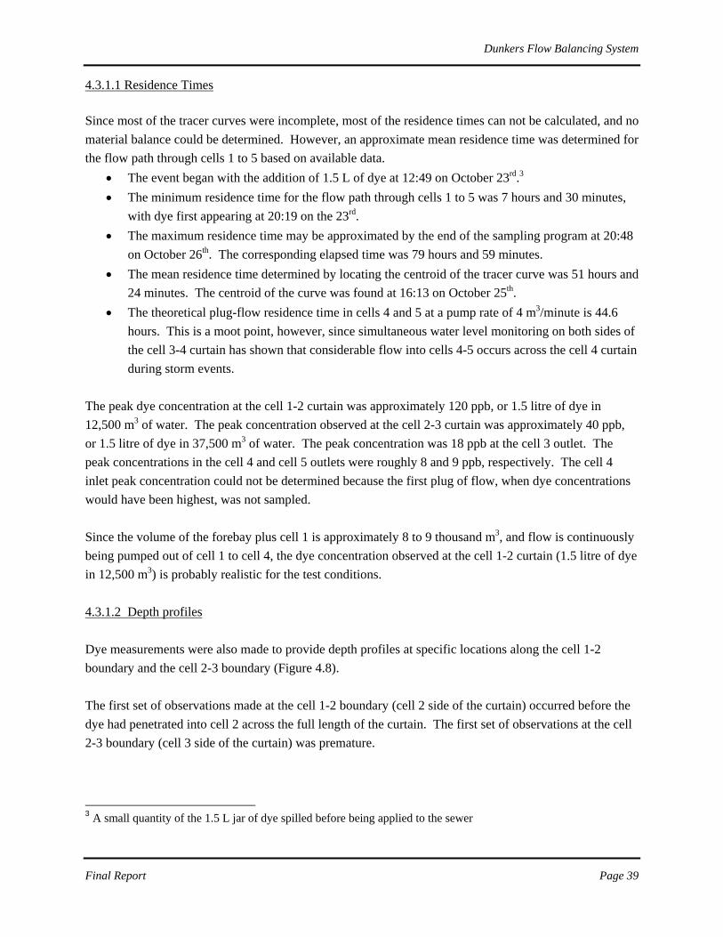
Dunkers Flow Balancing System
Final Report Page 39
4.3.1.1 Residence Times Since most of the tracer curves were incomplete, most of the residence times can not be calculated, and no material balance could be determined. However, an approximate mean residence time was determined for the flow path through cells 1 to 5 based on available data.
• The event began with the addition of 1.5 L of dye at 12:49 on October 23rd.3
3 A small quantity of the 1.5 L jar of dye spilled before being applied to the sewer
• The minimum residence time for the flow path through cells 1 to 5 was 7 hours and 30 minutes, with dye first appearing at 20:19 on the 23rd.
• The maximum residence time may be approximated by the end of the sampling program at 20:48 on October 26th. The corresponding elapsed time was 79 hours and 59 minutes.
• The mean residence time determined by locating the centroid of the tracer curve was 51 hours and 24 minutes. The centroid of the curve was found at 16:13 on October 25th.
• The theoretical plug-flow residence time in cells 4 and 5 at a pump rate of 4 m3/minute is 44.6 hours. This is a moot point, however, since simultaneous water level monitoring on both sides of the cell 3-4 curtain has shown that considerable flow into cells 4-5 occurs across the cell 4 curtain during storm events.
The peak dye concentration at the cell 1-2 curtain was approximately 120 ppb, or 1.5 litre of dye in 12,500 m3 of water. The peak concentration observed at the cell 2-3 curtain was approximately 40 ppb, or 1.5 litre of dye in 37,500 m3 of water. The peak concentration was 18 ppb at the cell 3 outlet. The peak concentrations in the cell 4 and cell 5 outlets were roughly 8 and 9 ppb, respectively. The cell 4 inlet peak concentration could not be determined because the first plug of flow, when dye concentrations would have been highest, was not sampled. Since the volume of the forebay plus cell 1 is approximately 8 to 9 thousand m3, and flow is continuously being pumped out of cell 1 to cell 4, the dye concentration observed at the cell 1-2 curtain (1.5 litre of dye in 12,500 m3) is probably realistic for the test conditions. 4.3.1.2 Depth profiles Dye measurements were also made to provide depth profiles at specific locations along the cell 1-2 boundary and the cell 2-3 boundary (Figure 4.8). The first set of observations made at the cell 1-2 boundary (cell 2 side of the curtain) occurred before the dye had penetrated into cell 2 across the full length of the curtain. The first set of observations at the cell 2-3 boundary (cell 3 side of the curtain) was premature.
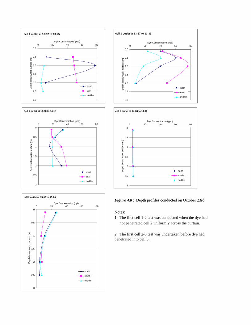
Figure 4.8 : Depth profiles conducted on October 23rd
Notes:1. The first cell 1-2 test was conducted when the dye had not penetrated cell 2 uniformly across the curtain.
2. The first cell 2-3 test was undertaken before dye had penetrated into cell 3.
cell 1 outlet at 13:12 to 13:25
0.0
0.5
1.0
1.5
2.0
2.5
3.0
0 20 40 60 80Dye Concentration (ppb)
Dep
th b
elow
wat
er s
urfa
ce (m
)
west
east
middle
cell 1 outlet at 13:27 to 13:39
0.0
0.5
1.0
1.5
2.0
2.5
3.0
0 20 40 60 80Dye Concentration (ppb)
Dep
th b
elow
wat
er s
urfa
ce (m
)
west
east
middle
Cell 1 outlet at 14:08 to 14:18
0
0.5
1
1.5
2
2.5
3
0 20 40 60 80Dye Concentration (ppb)
Dep
th b
elow
wat
er s
urfa
ce (m
)
west
east
middle
cell 2 outlet at 14:08 to 14:18
0
0.5
1
1.5
2
2.5
3
0 20 40 60 80Dye Concentration (ppb)
Dep
th b
elow
wat
er s
urfa
ce (m
)
north
south
middle
cell 2 outlet at 15:03 to 15:20
0
0.5
1
1.5
2
2.5
3
0 20 40 60 80Dye Concentration (ppb)
Dep
th b
elow
wat
er s
urfa
ce (m
)
north
south
middle

Dunkers Flow Balancing System
Final Report Page 41
The depth profiles suggest that the dye (i.e., the influent) initially moves across the top of the cell contents, which is consistent with earlier observations. While the new fluid remains in the system, and the farther it moves through the system, it tends to sink toward the bottom. This effect is probably influenced by system geometry, inertia and temperature/density factors. Since the influent enters the system near the surface, inertia will tend to keep it there, as long as structures are not put in place to create a more uniform vertical distribution. The curtains that were designed to restrict and distribute flow consist of vertical panels with spaces between them. The spaces extend from the pontoons to the bottom of the cells and would not be expected to impose much vertical redistribution of the flow. If the influent were warmer than the system contents, it would tend to remain on top, assuming that the temperatures are above the maximum density point of 4°C. If the influent is colder than the cell contents, or when it cools, it will eventually sink to the bottom. Temperature data were not available for the date of the dye test; the record stops on October 18th in 2001. The records show that the influent was colder than the pond contents prior to October 9, but warmer than the pond contents after that date. However, most of that data pertained to baseline or dry-weather flow.4 4.3.1.3 Summary The wet weather dye test showed that for a 7.1 mm event with a maximum intensity of 6.7 mm/hr, the facility was effective in retaining the influent for at least seven hours before measurable discharge through one or both of the outlets occurred. This 7 hour period roughly corresponds to the initial period during which the facility water levels were elevated above baseflow levels (i.e. the period of high discharge to receiving waters). Once dye started to be detected at the cell 3 outlet, effluent flows had returned to baseflow levels and thus pollutant loading rates would have been small. Upon first inspection, the dispersion patterns through the forebay, cell 1 and cell 2 were consistent with the principle of establishing plug-flow-like conditions with the displacement of cell contents by the new influent flow. However, the combination of depth profiles and consideration of the runoff volume indicate that the influent flow can not be well-distributed vertically, such that some of the influent flow exits the cells before all of the current contents have been displaced. This observation is consistent with simple volume displacement calculations. Approximately 3,300 m3 of stormwater was discharged during the event. If the new water simply displaced the contents of each cell sequentially, then it would not have moved further than cell 1, which has a volume of 7,900 m3. Instead, the dye is observed to penetrate through cell 2 and into cell 3 (combined volume of cell 1 and 2 is approximately 17,300 m3) before the end of the runoff event.
4 Season 2002 observations include continuous depth-profiles of water temperature (see sections 4.4, 4.4.5 and Appendix G).
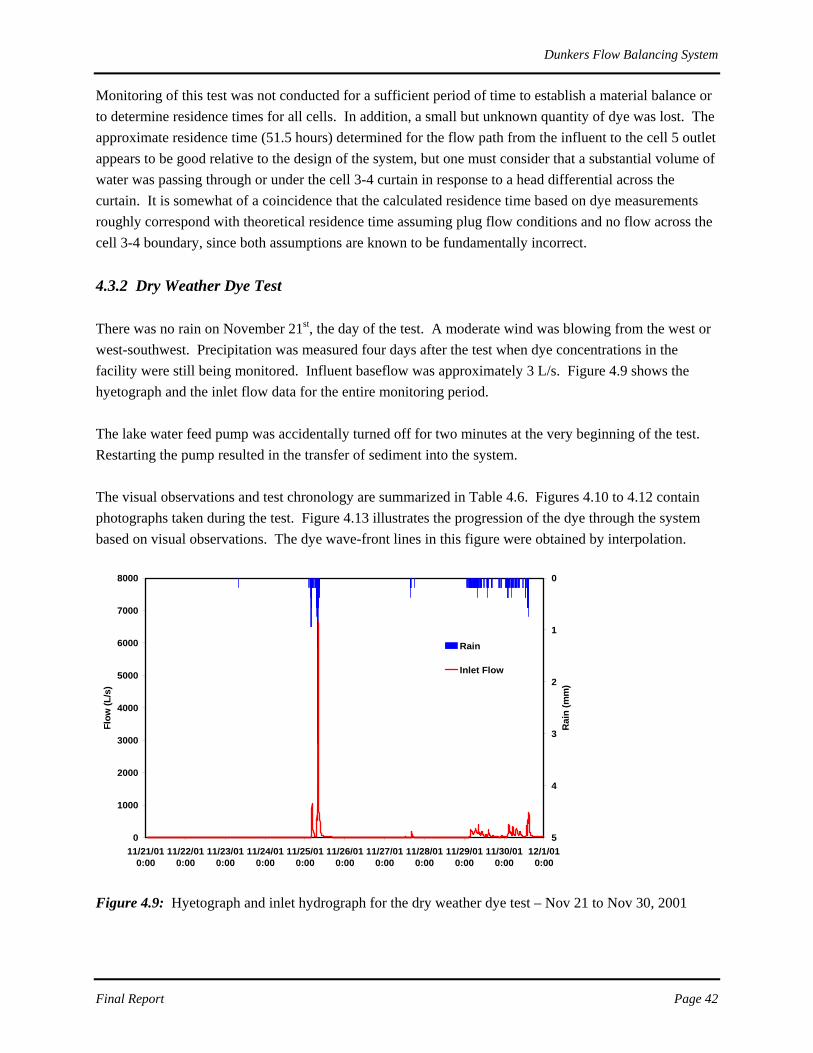
Dunkers Flow Balancing System
Final Report Page 42
Monitoring of this test was not conducted for a sufficient period of time to establish a material balance or to determine residence times for all cells. In addition, a small but unknown quantity of dye was lost. The approximate residence time (51.5 hours) determined for the flow path from the influent to the cell 5 outlet appears to be good relative to the design of the system, but one must consider that a substantial volume of water was passing through or under the cell 3-4 curtain in response to a head differential across the curtain. It is somewhat of a coincidence that the calculated residence time based on dye measurements roughly correspond with theoretical residence time assuming plug flow conditions and no flow across the cell 3-4 boundary, since both assumptions are known to be fundamentally incorrect. 4.3.2 Dry Weather Dye Test There was no rain on November 21st, the day of the test. A moderate wind was blowing from the west or west-southwest. Precipitation was measured four days after the test when dye concentrations in the facility were still being monitored. Influent baseflow was approximately 3 L/s. Figure 4.9 shows the hyetograph and the inlet flow data for the entire monitoring period. The lake water feed pump was accidentally turned off for two minutes at the very beginning of the test. Restarting the pump resulted in the transfer of sediment into the system. The visual observations and test chronology are summarized in Table 4.6. Figures 4.10 to 4.12 contain photographs taken during the test. Figure 4.13 illustrates the progression of the dye through the system based on visual observations. The dye wave-front lines in this figure were obtained by interpolation.
0
1000
2000
3000
4000
5000
6000
7000
8000
11/21/010:00
11/22/010:00
11/23/010:00
11/24/010:00
11/25/010:00
11/26/010:00
11/27/010:00
11/28/010:00
11/29/010:00
11/30/010:00
12/1/010:00
Flow
(L/s
)
0
1
2
3
4
5
Rai
n (m
m)
Rain
Inlet Flow
Figure 4.9: Hyetograph and inlet hydrograph for the dry weather dye test – Nov 21 to Nov 30, 2001

Dunkers Flow Balancing System
Final Report Page 43
Table 4.6: Dye test observations and key to photographs Elapsed Time
Time* Description
00:00 10:00 Two litres of dye was injected into the lake water entering cell 3 00:00 10:00 Dye was injected into the lake water entering cell 3 (close-up). The dye is spreading
radially with some bias toward the east. Turbulence is causing foam formation. 00:01 10:01 Photo of dye moving eastward along the south shore in cell 3 10:05 The lake water feed pump was accidentally shut off for 2 minutes. 00:09 10:09 Photo of dye about ½ way to the cell 2-3 curtain. 10:10 10:10 Red foam has floated/blown to the cell 2-3 curtain. 00:32 10:32 Photo of dye reaching the cell 2-3 curtain, still mostly along the south shore 00:34 10:34 (close-up, similar to previous) 10:40 10:40 Dye enters cell 2. 00:41 10:41 Dye moves diagonally (north-westerly) toward the cell 3 outlet. This flow pattern
may indicate an interaction with the dry-weather baseflow. 00:51 10:51 Photo of dye distribution pattern in cell 3 00:51 10:51 Close-up photo of the dye entering cell 2 00:58 10:58 Similar to previous photo 01:38 11:38 Dye dispersion in cells 2 and 3 01:39 11:39 Dye pattern along the south shore of cell 2 01:45 11:45 Dye dispersion in cells 2 and 3 01:47 11:47 Dye moves along the east shore of cell 2 01:52 11:52 Dye diffusion increases in cell 3 01:53 11:53 Dye moves along the south and east shores of cell 2 02:06 12:06 Dye is in the vicinity of the mud flat
Dye has reached the cell 1-2 curtain at the westerly end. 02:25 12:25 Dye exits cell 3 to the outlet channel. 02:32 12:32 Dye leaves cell 3 through the outlet gate 02:35 12:35 Dye is observed in the cell 3 outlet channel 02:39 12:39 Dye enters cell 1 02:49 12:49 Dye enters the mud flat 03:00 13:00 Dye moves westward along the cell 1-2 curtain 03:46 13:46 Dye spreads throughout cell 2 04:17 14:17 Dye is well-distributed in cell 3 04:37 14:37 Same as previous 04:39 14:39 Photos (almost identical) of cells 1 and 2, with faint colour but good dispersion in
cell 2 and possibly some colour in cell 1 04:45 14:45 Dye is well-dispersed in cell 3 26:09 Nov 22 Photos taken on November 22nd show good dye dispersion in cells 1, 2 and 3, with
possibly a trace of dye in cells 4 and 5 * Selected photos shown in figures 4.10 to 4.12 are bolded; additional digital photographs available on file but not
shown are italicized.

Figure 4.10: Photographs of dye in cell 3 - first few minutes of test Notes: 1. These photographs were taken looking southward. 2. Dye was added at the holding well between the lake and cell 3 at
10:00.

Figure 4.11: Photographs of dye approaching the cell 2-3 curtain Notes:
1. Dye was observed entering cell 2 adjacent to the south shore at 10:40.
2. The sampler on the cell 2-3 pontoon, with its intake located on the cell 2 side of the curtain, first detected a concentration above baseline at 11:50.
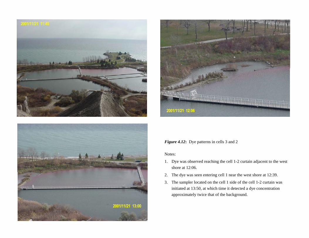
Figure 4.12: Dye patterns in cells 3 and 2 Notes:
1. Dye was observed reaching the cell 1-2 curtain adjacent to the west shore at 12:06.
2. The dye was seen entering cell 1 near the west shore at 12:39.
3. The sampler located on the cell 1 side of the cell 1-2 curtain was initiated at 13:50, at which time it detected a dye concentration approximately twice that of the background.

Dunkers Flow Balancing System
Final Report Page 47
Figure 4.13: Interpolated dye wavefronts The principal visual observations were:
• Shortly after addition, the dye moved easterly along the south shore of cell 3, and moved north toward the centre of cell 3 at a slower rate. Some dye-bearing foam was blown in an easterly direction, reaching the cell 2-3 curtain 10 minutes after dye addition.
• The dye reached the cell 2-3 curtain after 40 minutes, still predominantly adjacent to the south shore of cell 3.
• The dye moved east in cell 2, remaining close to the south shore, then moved northerly following the east shore. There was no visual evidence of dye migrating toward the centre of cell 2.
• The dye required 86 minutes to travel between the cell 2-3 curtain and the cell 1-2 curtain (2 hr. 6 min. elapsed time).
• Upon reaching the cell 1-2 curtain, the dye moved west along the curtain. No dye was seen in cell 1 until approximately 30 minutes after it had reached the cell 2 side of the cell 1-2 curtain.

Dunkers Flow Balancing System
Final Report Page 48
• In cell 3, over a time period of about two hours, some dye was seen moving north from the point of addition in the general direction of the north end of the cell 3 outlet structure. After approximately 2 ½ hours, some dye was observed in the outlet channel.
The flow patterns observed in cells 2 and 3 are interesting. Conceptually, there are two opposing flows during dry weather. One flow consists of the lake water entering cell 3 at 67 L/s and moving to cell 1 where water is pumped at the same rate into cell 4. The second flow consists of a smaller dry-weather flow, at an average rate of approximately 3 L/s, which moves from the inlet structure, through cells 1 to 3 and into the lake. Obviously, these flows will mix to some extent but the dominant flow will be from the much greater volume of lake water entering cell 3. The relative temperatures of the pond contents, the lake water, pumping at cell 4 and the influent water would all be expected to influence the flow patterns. Wind is also a significant factor.5
5 It is conceivable that if wind were from the east instead of the west, much more of the dye (i.e. lake water) would have exited through the cell 3 outlet. Higher influent baseflows would also contribute to this result.
The circular flow pattern in cell 2 may have resulted from the near-shore (tangential) input(s) reinforced by the coriolis effect. However, when considering the pumping rate, the apparent reluctance of the dye to enter cell 1 is unexpected. Perhaps a circular flow similar to that observed in cell 2 is occurring in cell 1, causing a tangential flow on both sides of the cell 1-2 curtain. The combination of influent flow directed into the centre of cell 1, wind from the west, and pumping of water near the east shore of the cell may encourage a circular flow pattern. The gaps in the curtain would be expected to distribute the flow and, hence, would also have contributed to the dispersion along the length of the curtain. The dye tracer concentrations are presented in Figure 4.14. The sampler intake locations used for this test were the same as those employed for the monitoring of runoff events, as illustrated in Figure 2.3. The cell 3 sample station was intended to represent the outlet water quality. The sampler intake was located at the mid-point of the outlet gate structure, and about 4 metres upstream of the gate. The offset was chosen to avoid possible turbulence and sediment resuspension at the shallow end of cell 3 when sampling runoff events. Although visual observations showed a slow progression of dye toward the outlet, the sampler intake was located relatively close to the dye plume and has measured significant concentrations of dye. Sampling was continued until mid-December using a combination of automated and grab sampling techniques. A discussion of the results follows:
• There was a progression of concentration peaks between cells 2 and 1, with the latter curve being broader and having a lower peak, as would be expected.
• The cell 4 influent curve, the cell 4 effluent curve and the cell 5 effluent curve initially have the relative shapes that may be expected for this system.
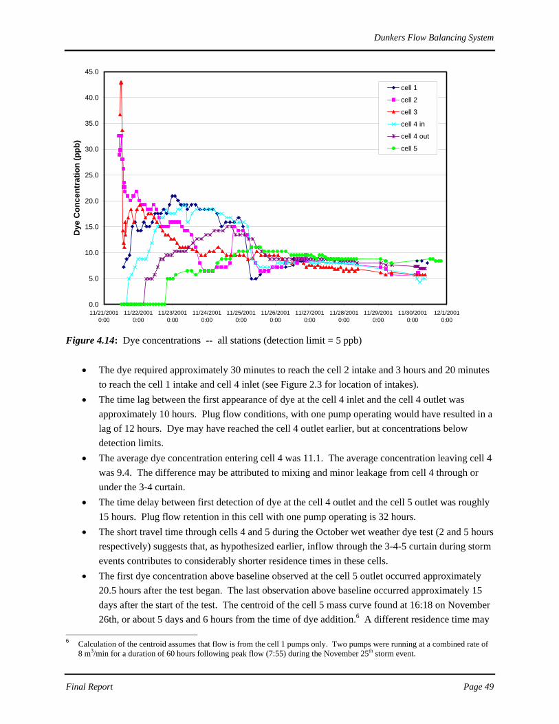
Dunkers Flow Balancing System
Final Report Page 49
0.0
5.0
10.0
15.0
20.0
25.0
30.0
35.0
40.0
45.0
11/21/20010:00
11/22/20010:00
11/23/20010:00
11/24/20010:00
11/25/20010:00
11/26/20010:00
11/27/20010:00
11/28/20010:00
11/29/20010:00
11/30/20010:00
12/1/20010:00
Dye
Con
cent
ratio
n (p
pb)
cell 1
cell 2
cell 3
cell 4 in
cell 4 out
cell 5
Figure 4.14: Dye concentrations -- all stations (detection limit = 5 ppb)
• The dye required approximately 30 minutes to reach the cell 2 intake and 3 hours and 20 minutes to reach the cell 1 intake and cell 4 inlet (see Figure 2.3 for location of intakes).
• The time lag between the first appearance of dye at the cell 4 inlet and the cell 4 outlet was approximately 10 hours. Plug flow conditions, with one pump operating would have resulted in a lag of 12 hours. Dye may have reached the cell 4 outlet earlier, but at concentrations below detection limits.
• The average dye concentration entering cell 4 was 11.1. The average concentration leaving cell 4 was 9.4. The difference may be attributed to mixing and minor leakage from cell 4 through or under the 3-4 curtain.
• The time delay between first detection of dye at the cell 4 outlet and the cell 5 outlet was roughly 15 hours. Plug flow retention in this cell with one pump operating is 32 hours.
• The short travel time through cells 4 and 5 during the October wet weather dye test (2 and 5 hours respectively) suggests that, as hypothesized earlier, inflow through the 3-4-5 curtain during storm events contributes to considerably shorter residence times in these cells.
• The first dye concentration above baseline observed at the cell 5 outlet occurred approximately 20.5 hours after the test began. The last observation above baseline occurred approximately 15 days after the start of the test. The centroid of the cell 5 mass curve found at 16:18 on November 26th, or about 5 days and 6 hours from the time of dye addition.6 A different residence time may
6 Calculation of the centroid assumes that flow is from the cell 1 pumps only. Two pumps were running at a combined rate of
8 m3/min for a duration of 60 hours following peak flow (7:55) during the November 25th storm event.

Dunkers Flow Balancing System
Final Report Page 50
have resulted if there had been no rain during the monitoring period. Theoretical plug flow conditions through cells 3, 2, 1, 4 and 5 at a flow rate of 4 m3/minute would result in a residence time of 6.8 days.
• Samples collected up to November 30th indicated significant residual concentrations at all locations except possibly cell 1. Grab samples collected at the cell 3 and cell 5 outlets on December 4th, 6th and 13th indicated that the dye concentrations did eventually return to baseline conditions, but only after 22 days.
4.3.2.1 Depth Profiles Dye concentration depth profiles were also measured at 3 intervals along the cell 2-3 and cell 1-2 curtain (Figure 4.15). Initially, the dye approaching cell 2 was concentrated at mid-depth on the cell 3 side of the curtain. Twenty minutes later, on the cell 2 side of the curtain, dye was more concentrated near the surface. Later observations in cells 1 and 2 showed fairly uniform depth distributions. 4.3.2.2 Rain Events Figure 4.17 shows the movement of dye within the facility in response to the rain event on the 25th of November, almost 4 days after dye injection. Total rainfall and flow during this event was 25.2 mm and 15,000 m3, respectively . A second pump at cell 1 was triggered at 7:55 for a period of 60 hours when the peak inflow rate exceeded 4000 L/s causing the pumping rate to increase from 67 to 133 L/s. The influent runoff flushed the residual dye out of cells 1 and 2. Consequently, the dye concentration in these cells and the cell 4 influent decreased suddenly. The displacement of dye from cells 1 and 2 resulted in a minor increase in dye concentration at the cell 3 outlet station. Mixing of new and old water may explain subsequent decreases in dye concentrations at 3 and the cell 4 and 5 outlets. Identical water levels on either side of the cell 3-4-5 curtain indicated that considerable flow through or under the curtain was occurring throughout the event. After facility water levels had reached a steady state, the dye stored in cell 3 was subsequently drawn back into cells 2, 1 and 4 as seen by a concentration decrease in cell 3, and concentration increases at the other monitoring stations. During this period, water was being transferred from cell 1 to cell 4 at double the rate that lake water was entering cell 3, resulting in a stronger reverse hydraulic gradient than would have been the case if only one pump was running. The dye concentrations in cells 1 and 2 can also be seen to respond in a similar fashion to the much smaller rainfall events on November 29th and November 30th.

Figure 4.15 : Dye tracer depth profiles -- dry weather test
Notes:1. The first set of observations was made on the cell 3 side of the cell 2-3 curtain.2. All other cell 2 observations were made on the cell 2 side of the cell 2-3 curtain.3. The cell 1 observations were made on the cell 1 side of the cell 1-2 curtain.
cell 3 10:42 to 10:49
0
0.5
1
1.5
2
2.5
3
0 10 20 30 40 50 60 70 80 90
Dye Concentration (ppb)
Dep
th b
elow
wat
er s
urfa
ce (m
)
south
cell 2 at 11:08 to 11:15
0
0.5
1
1.5
2
2.5
3
0 10 20 30 40 50 60 70 80 90Dye Concentration (ppb)
Dep
th b
elow
wat
er s
urfa
ce (m
)
south
middle
cell 2 at 12:35 to 12:45
0
0.5
1
1.5
2
2.5
3
0 10 20 30 40 50 60 70 80 90Dye Concentration (ppb)
Dep
th b
elow
wat
er s
urfa
ce (m
)
south
middle
north
cell 2 at 13:58 to 14:05
0
0.5
1
1.5
2
2.5
3
0 10 20 30 40 50 60 70 80 90Dye Concentration (ppb)
Dep
th b
elow
wat
er s
urfa
ce (m
)
south
middle
north
cell 1 at 14:23 to 14:30
0
0.5
1
1.5
2
2.5
3
0 10 20 30 40 50 60 70 80 90Dye Concentration (ppb)
Dep
th b
elow
wat
er s
urfa
ce (m
)
west
middle
east
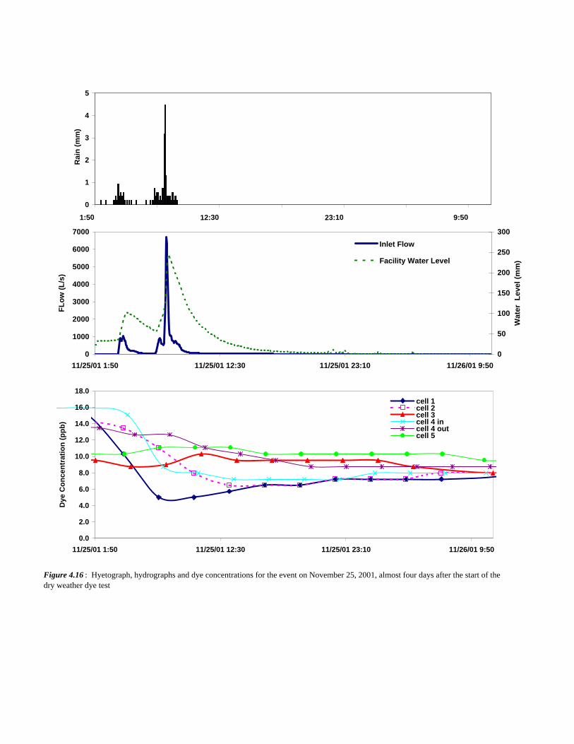
Figure 4.16 : Hyetograph, hydrographs and dye concentrations for the event on November 25, 2001, almost four days after the start of the dry weather dye test
0.0
2.0
4.0
6.0
8.0
10.0
12.0
14.0
16.0
18.0
11/25/01 1:50 11/25/01 12:30 11/25/01 23:10 11/26/01 9:50
Dye
Con
cent
ratio
n (p
pb)
cell 1cell 2cell 3cell 4 incell 4 outcell 5
0
1000
2000
3000
4000
5000
6000
7000
11/25/01 1:50 11/25/01 12:30 11/25/01 23:10 11/26/01 9:50
FLow
(L/s
)
0
50
100
150
200
250
300
Wat
er L
evel
(mm
)
Inlet Flow
Facility Water Level
0
1
2
3
4
5
1:50 12:30 23:10 9:50
Rai
n (m
m)

Dunkers Flow Balancing System
Final Report Page 53
4.3.2.3 Summary The dry-weather and wet-weather flow patterns observed in the dye test demonstrated that the facility was performing generally as intended, retaining runoff and processing it through cells 4 and 5. Visual observations and dye concentration measurements indicated significant departure from plug flow conditions. Dye was first detected at cell 5 less than a day after the start of the test, and continued to be detected 15 days later. At a pump rate of 4 m3/minute, theoretical plug flow through cells 3, 2, 1, 4 and 5 would result in a residence time of 6.8 days. The dye patterns observed in cells 3 and 2 confirmed that the hydraulic conditions were very complex. The hydraulic performance of cell 4 - based on initial lag time and average concentrations – was considerably longer than observed during the wet weather dye test. After dye was first detected at the cell 4 inlet, approximately 10 hours passed before it first appeared at the cell 4 outlet. Plug flow conditions, with one pump operating indicate a theoretical lag time of 12 hours. The short travel time through cells 4 during the October wet weather dye test (2 hours) suggests that, as hypothesized earlier, inflow through the 3-4 curtain during storm events contributes to considerably shorter residence times in these cells. The dry-weather flow from the sewer system and the pumped flow appear to remain separate to a large extent. Hence, the dry-weather flow would be expected to displace some of the stormwater from the storage cells into the lake through the cell 3 outlet gate. Simultaneously, the pumped lake water would be displacing stored stormwater toward cell 1 for transfer to cells 4 and 5. Some pumped lake water would intermix with the dry-weather flow and the stored stormwater, diluting the effluent from cell 3, but the amount of intermixing appears to be minor. Although this test did not provide exclusively dry-weather data, the system’s response to the rain event of November 25th was very informative. Analysis suggested that during a large event of this nature, the facility was effective in storing most of the new influent water. This interpretation is consistent with the analysis of discrete suspended solids data discussed in later in this chapter. After the event, the displaced residual dye in cells 1 and 2 was subsequently returned to cell 1 and transferred to cells 4 and 5 by pumping. If additional dye tests are to be conducted, tracing of the dry-weather flow by adding dye to the influent would be informative. Different dyes may be considered for the influent and lake water in a simultaneous test of the two streams, assuming that the dyes can be measured at different wavelengths in a common sample. An additional change is recommended: the cell 3 effluent should be sampled in the outlet channel to avoid sampling the lake water plume in cell 3.
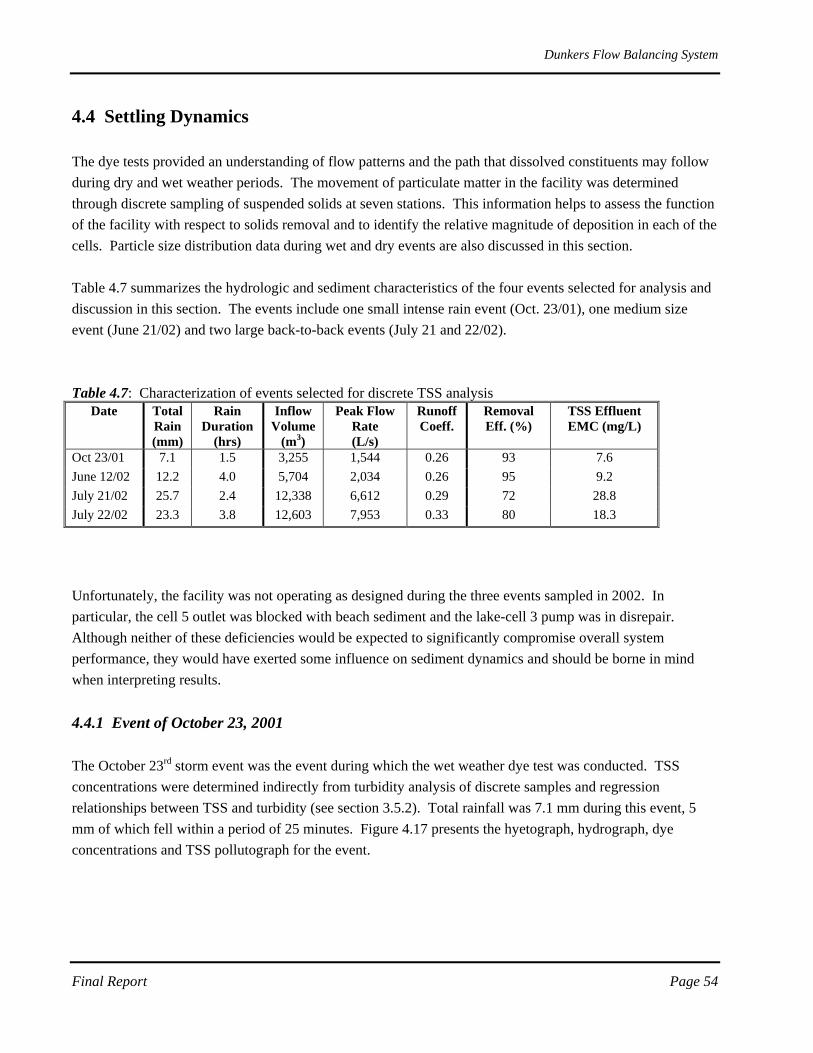
Dunkers Flow Balancing System
Final Report Page 54
4.4 Settling Dynamics The dye tests provided an understanding of flow patterns and the path that dissolved constituents may follow during dry and wet weather periods. The movement of particulate matter in the facility was determined through discrete sampling of suspended solids at seven stations. This information helps to assess the function of the facility with respect to solids removal and to identify the relative magnitude of deposition in each of the cells. Particle size distribution data during wet and dry events are also discussed in this section. Table 4.7 summarizes the hydrologic and sediment characteristics of the four events selected for analysis and discussion in this section. The events include one small intense rain event (Oct. 23/01), one medium size event (June 21/02) and two large back-to-back events (July 21 and 22/02). Table 4.7: Characterization of events selected for discrete TSS analysis
Date Total Rain (mm)
Rain Duration
(hrs)
Inflow Volume
(m3)
Peak Flow Rate (L/s)
Runoff Coeff.
Removal Eff. (%)
TSS Effluent EMC (mg/L)
Oct 23/01 7.1 1.5 3,255 1,544 0.26 93 7.6 June 12/02 12.2 4.0 5,704 2,034 0.26 95 9.2 July 21/02 25.7 2.4 12,338 6,612 0.29 72 28.8 July 22/02 23.3 3.8 12,603 7,953 0.33 80 18.3
Unfortunately, the facility was not operating as designed during the three events sampled in 2002. In particular, the cell 5 outlet was blocked with beach sediment and the lake-cell 3 pump was in disrepair. Although neither of these deficiencies would be expected to significantly compromise overall system performance, they would have exerted some influence on sediment dynamics and should be borne in mind when interpreting results. 4.4.1 Event of October 23, 2001 The October 23rd storm event was the event during which the wet weather dye test was conducted. TSS concentrations were determined indirectly from turbidity analysis of discrete samples and regression relationships between TSS and turbidity (see section 3.5.2). Total rainfall was 7.1 mm during this event, 5 mm of which fell within a period of 25 minutes. Figure 4.17 presents the hyetograph, hydrograph, dye concentrations and TSS pollutograph for the event.

Figure 4.17 : Hyetograph, hydrograph, dye and TSS concentrations for the event on October 23rd, 2001
0
20
40
60
80
100
120
140
160
180
200
12:15 12:55 13:35 14:15 14:55 15:35 16:15 16:55 17:35 18:15 18:55
TSS
Con
cent
ratio
n (m
g/L)
Inlet Cell 1 Cell 2
Cell 4 in Cell 4 out Cell 3
0
0.5
1
1.5
2
2.5
12:15 12:55 13:35 14:15 14:55 15:35 16:15 16:55 17:35 18:15 18:55
Rai
n (m
m)
0
10
20
30
40
50
60
70
80
90
100
110
120
130
12:15 12:55 13:35 14:15 14:55 15:35 16:15 16:55 17:35 18:15 18:55
Dye
Con
cent
ratio
n (p
pb)
Cell 1 Cell 2
Cell 4 in Cell 4 out
Cell 3 cell 5
0
250
500
750
1000
1250
1500
1750
12:15 12:55 13:35 14:15 14:55 15:35 16:15 16:55 17:35 18:15 18:55
FLow
(L/s
)
0
20
40
60
80
100
120
140
Wat
er L
evel
(mm
)
flow
water level

Dunkers Flow Balancing System
Final Report Page 56
The influent hydrograph and pollutograph peaked simultaneously, resulting in a flow weighted mean influent concentration for the event of 116 mg/L. Water levels peaked approximately 1 hour after the peak of the inflow hydrograph, and at roughly the same time as the peak of the cell 1 TSS pollutograph. The dye and suspended solids concentrations at the cell 1 station showed a similar pattern during the first 2 hours of runoff. After this time, TSS concentrations in cell 1 declined considerably, whereas the dissolved dye increased slightly and remained at higher levels relative to baseline, as would be expected. Under strict plug flow conditions (i.e. no mixing), the entire inflow volume from the storm (3220 m3) would have been captured in cell 1 (volume = 7900 m3), and there would have been no evidence of suspended solids or dye in cell 2. In reality, however, there is considerably mixing between new influent and stored water, and not all of the available storage is being used to maximum effect. Therefore, it is not surprising to see a modest jump in suspended solids at the cell 2 outlet after the first two hours of the storm. The similarity of the observed concentrations to those in cell 1, and the extended length of the peak suggest that the cell 2 concentrations are comprised primarily of relatively fine particles that settle out of suspension only under highly quiescent conditions. Dye concentrations in cell 2 experience a rapid rise about 20 minutes after the jump in cell 2 TSS concentrations, although the first signs of dye at the monitoring location occurred roughly an hour earlier. The cell 4 inlet sampler malfunctioned during the storm and had to be initiated manually, resulting in a significant delay in sample collection. TSS concentrations at this station during the last three hours of outflow were in the same range as at the cell 1 and 2 stations. Dye concentrations at the cell 4 inlet were lower than at the other two stations over the same period. Since the intake to the cell 4 inlet pump is located near the bottom of cell 1, upstream of the cell 1 intake, it may be assumed that the dissolved dye, which is not subject to settling, was more concentrated near the surface. The cell 3 outlet showed no significant change in TSS concentrations. This was also true of the cell 4 outlet, although dye concentrations at that location show a minor increase about 3 hours after the start of runoff. Turbidity measurements were not measured on cell 5 samples, but TSS concentrations of 4 composite samples collected during and two days after the event were not significantly different. 4.4.2 Event of June 21, 2002 Figure 4.18 shows the hydrographs, pollutographs and a depth profile of water temperature during the June 21st event. The temperature depth profile was measured on the downstream side of the cell 1-2 curtain near the centre. This event had 12.2 mm of rain distributed as three peaks approximately one hour and 30 minutes apart. Approximately 67% of the total mass of suspended solids was discharged over the first 30 minutes of the storm. The flow weighted influent TSS concentration for the event was 197 mg/L.

Figure 4.18 : hyetograph, hydrographs, TSS concentrations and depth profiles of temperature at the cell 1-2 curtain for the event on June 21, 2002
0
1
2
3
4
5
6
15:55 16:35 17:15 17:55 18:35 19:15 19:55 20:35 21:15 21:55 22:35 23:15 23:55
Rai
n (m
m)
0
50
100
150
200
250
300
350
400
450
15:55 16:35 17:15 17:55 18:35 19:15 19:55 20:35 21:15 21:55 22:35 23:15 23:55
TSS
Con
cent
ratio
n (m
g/L)
Inlet Cell 1
Cell 2 Cell 3
Cell 4 in
15
17
19
21
23
25
27
15:55 16:35 17:15 17:55 18:35 19:15 19:55 20:35 21:15 21:55 22:35 23:15 23:55
Wat
er T
empe
ratu
re(D
egre
es C
elsi
us)
surface depth (0.5 m)mid depth (1.5 m)bottom depth (2.5 m)
0
500
1000
1500
2000
15:55 16:35 17:15 17:55 18:35 19:15 19:55 20:35 21:15 21:55 22:35 23:15 23:55
FLow
(L/s
)
0
20
40
60
80
100
120
140
160
Wat
er L
evel
(mm
)
flow
Facility Water Level

Dunkers Flow Balancing System
Final Report Page 58
Lake levels were above the concrete sill of the cell 3 outlet weir during this event. Prior to the event, lake water was flowing into the facility through the cell 3 weir, as seen by the rising facility water levels. Event runoff reversed the direction of flow from the lake into the facility to the facility out to the lake.6 Over the course of the event, lake waters decreased by about 2 cm below pre-event levels, then started to increase again. Cell 1 was the only station within the facility that showed distinct variations in discrete TSS concentrations. The peak concentration at this station occurred 23 minutes after the influent peak and corresponded with the maximum facility water level. The absence of a similar rise in TSS concentrations at the cell 4 inlet station suggests that new runoff may have short circuited across the top of the cell. The relatively constant temperatures at the 1.5 and 2.5 m depths during the initial stages of the storm lend support to this interpretation. After the second plug of flow, a small but distinguishable rise in TSS concentrations can be observed at the cell 4 inlet and the cell 2 outlet. A small change in cell 2 inlet water temperatures (all depths) can be observed at roughly the same time. Overall, however, the pre-event thermal stratification is maintained throughout the event, suggesting minimal vertical mixing. The absence of any change in cell 3 concentrations indicates that the entire influent volume (5,704 m3) was stored and treated. 4.4.3 Event of July 21, 2002 During the July 21st event, 26 mm of rain fell over a period of 2 hours and 25 minutes (Figure 4.19). The total flow volume of 12,338 m3 was sufficient to fill all of cell 1 (7900 m3) and part of cell 2 (9400 m3). The second pump transferring water to cell 4 was automatically triggered 1 hour and 15 minutes after the initiation of runoff, in response to peak inflow exceeding 4000 L/s. The second pump remained on for 60 hours. The combined transfer rate of the two pumps to cell 4 was 8 m3/min or 480 m3/hour.7 A mass based analysis of this event and a second large event occurring on the following day is provided in Appendix D. The influent hydrograph had two peaks occurring one hour and 20 minutes apart. Mass loading of suspended solids was greatest during the second hydrograph peak. The mean flow weighted influent TSS concentration for the event was 104 mg/L.
6 The cell 3 gates swing out towards the lake to protect the facility from storm surges, but water can still enter at the interface between the gate and concrete sill. The uneven response of water levels to runoff during this event may reflect the resistance that high lake levels exert on the gates. 7 Note that even with two pumps running, the total volume of water transferred to cell 4 during the period of runoff is less than 10% of the total inflow volume.

Figure 4.19 : Hyetograph, hydrographs, TSS concentrations and temperature depth profiles at the cell 1-2 curtain for the event on July 21, 2002
0
20
40
60
80
100
120
140
160
22:30 23:10 23:50 0:30 1:10 1:50 2:30 3:10 3:50 4:30 5:10 5:50
TSS
Con
cent
ratio
n (m
g/L)
Inlet Cell 1
Cell 2 Cell 3
Cell 4 in
0
1
2
3
4
5
6
22:30 23:10 23:50 0:30 1:10 1:50 2:30 3:10 3:50 4:30 5:10 5:50
Rai
n (m
m)
20
22
24
26
28
30
22:30 23:10 23:50 0:30 1:10 1:50 2:30 3:10 3:50 4:30 5:10 5:50
Cel
l 2 W
ater
Tem
pera
ture
(Deg
rees
Cel
sius
)
surface depth (0.5 m)mid depth (1.5 m)bottom depth (2.5 m)
0
1000
2000
3000
4000
5000
6000
7000
8000
22:30 23:10 23:50 0:30 1:10 1:50 2:30 3:10 3:50 4:30 5:10 5:50
InfL
ow (L
/s)
0
50
100
150
200
250
300
350
Wat
er L
evel
(mm
)
flow
Facility water level
Dunkers Flow Balancing System
Final Report Page 60
The peaks of the TSS pollutographs at the cell 4 inlet and cell 1 stations corresponded with peak water levels in the facility. The cell 2 pollutograph peaked 20 minutes later. As during the October 23rd event, the rise and fall of TSS concentrations at cell 2 were slower and less pronounced than in cell 1, suggesting a finer particle size distribution at this station. All of the effluent exited through cell 3. There was a gradual rise in cell 3 TSS concentrations from 15 to 30 mg/L during the initial stages of the storm. The cause of this early rise was probably related to the re-suspension of previously settled solids as the flow rate through the gates increased. Another jump in concentrations from 30 to 50 mg/L occurred later in the storm. It is tempting to attribute this increase to the effect of new influent water. However, the rise is brief and may be simply the result of wash off from the pontoons or suspended material from elsewhere in the facility (e.g. sediment ponds) that was mobilized during high flow. Although influent temperature was not measured, the cell 2 temperature response suggests an average influent temperature of roughly 23°C, which is lower than the pre-event 0.5 and 1.5 m temperatures in cell 2 and higher than the temperature at 2.5 m. The water temperature starts to change slowly after the first hour of flow. Sharp temperature fluctuations occur over a period of 43 minutes from 23:53 to 0:36, corresponding to the second and larger plug of stormwater runoff. The drop in surface water temperature corresponds with the peak in the cell 1 and cell 4 inlet suspended solids concentration. Temperatures stabilize 10 minutes earlier at the surface than at the two lower depths, suggesting marginally faster flow across the surface, but overall the flow appears to be well integrated vertically. Unlike the June 21st storm, temperatures continue to change until about 4:40 in the morning, when a stable, relatively well mixed equilibrium is reached. 4.4.4 Event of July 22, 2002 The July 22nd event arrived before inflow rates from the previous event had returned to baseflow levels. Another 23 mm of rain fell during this event, most of concentrated in a single hydrograph peak (Figure 4.20). Peak flow would have been sufficient to trigger the second pump at cell 1 but this was not necessary because the pump was still on from the previous event. Despite significant wash off from the earlier rain event, the first flush phenomenon was still recognizable. Within the facility, TSS pollutographs at the cell 4 inlet and cell 1 outlet peaked before the influent TSS peak. The peak of the cell 2 and 3 pollutographs occurred 0.7 and 2.3 hours later, respectively. In this case, the peaks may be interpreted as the progress of influent water as it travels through the system, a small portion of which is eventually discharged to the lake (also see mass based analysis in Appendix D).

Figure 4.20 : Hyetograph, hydrographs, TSS concentrations and temperature depth profiles at the cell 1-2 curtain for the event on July 22, 2002
0
1
2
3
4
5
6
14:40 15:20 16:00 16:40 17:20 18:00 18:40 19:20 20:00
Rai
n (m
m)
0
20
40
60
80
100
120
140
160
14:40 15:20 16:00 16:40 17:20 18:00 18:40 19:20 20:00
TSS
Con
cent
ratio
n (m
g/L)
Inlet
Cell 1
Cell 2
Cell 3
Cell 4 in
20
22
24
26
28
30
14:40 15:20 16:00 16:40 17:20 18:00 18:40 19:20 20:00
Wat
er T
empe
ratu
re
(Deg
rees
Cel
sius
)
surface depth (0.5 m)mid depth (1.5 m)bottom depth (2.5 m)
0
1000
2000
3000
4000
5000
6000
7000
8000
14:40 15:20 16:00 16:40 17:20 18:00 18:40 19:20 20:00
InfL
ow (L
/s)
0
50
100
150
200
250
300
350
Wat
er L
evel
(mm
)
flow
Facility Water Level

Dunkers Flow Balancing System
Final Report Page 62
Water temperatures at all depths in cell 2 respond (i.e. rise at 1.5 and 2.5 m and decline at 0.5 m) to the influent at the same time suggesting a plug flow that is relatively well integrated vertically. That the surface water temperature does not drop as far as during the previous event (26 vs 24 °C) may be explained by the timing of the events: the first event occurred in the early morning whereas this event occurred in the late afternoon, when influent temperatures would be expected to be warmer. 4.4.5 Particle size distributions
Figures 4.21 and 4.22 compare average particle size distributions at each of the monitoring stations during wet and dry weather. Only data from the 2000 monitoring season were available.8 Distributions for individual events are presented in Appendix E.
During wet weather, the average particle size distributions at cells 3, 4 and 5 were all significantly different than that of the inlet at the 95% confidence level. The median particle size was approximately 7.5 μm at the inlet, compared to 3.5 μm at the pump intake at cell 4 and 2 μm at the two outlets.9 Particle size ranges at the inlet and outlets were 0.17 - 175 and 0.17 - 30 μm, respectively, indicating that the system was effective in removing all particle sizes greater than 30 μm.
During dry weather, 6 of the 20 grab samples collected had particle concentrations less than that required to undertake particle size analysis by the method employed in the laboratory. Among the remaining samples, outlet and inlet average size distributions had high standard deviations and were not found to be significantly different at the 95% confidence level. The median particle size was approximately 5.5 and 2 μm at the inlet and two outlets, respectively. Note that the dry and wet median effluent particle sizes were both 2 μm. Other studies of detention basins conducted by SWAMP suggest that even with larger permanent pools and longer settling times, it is not practical to expect reductions beyond a median effluent particle size of 2 μm.
8 Samples were submitted for analysis of particle size during the 2001 and 2002 seasons, but after the 2000 monitoring season, the laboratory dramatically raised the threshold beyond which samples were considered to be too clear for analysis. Hence, only a small number of influent and cell 1 samples were analyzed. 9 An influent median particle size of 11 μm was used in the design of the facility (Aquafor Beech, 1994).

Figure 4.21: Average cumulative particle size distributions of wet weather samples collected from May 10 to November 16, 2000
Figure 4.22: Average cumulative particle size distributions of dry weather samples collected from May 10 to November 16, 2000
0
10
20
30
40
50
60
70
80
90
100
0.1 1 10 100 1000Particle Size (µm)
% G
reat
er T
han
INLET
CELL 3
CELL 4INLET
CELL 4OUTLET
CELL 5
LAKE
0
10
20
30
40
50
60
70
80
90
100
0.1 1 10 100 1000Particle Size (µm)
% G
reat
er T
han
INLET
CELL 3
CELL 4INLET
CELL 5
LAKE

Dunkers Flow Balancing System
Final Report Page 64
4.5 Water Quality
The following sections summarize water quality and temperature monitoring results for wet and dry weather, and during the post event period. Detailed water quality summary statistics are provided in Appendix F.
4.5.1 Wet weather concentrations 4.5.1.1 Effluent
Comparison of wet weather effluent concentrations with receiving water standards developed by government agencies for a range of water quality variables provides an indirect measure of the potential impact that facility discharges may have on the health of receiving waters with respect to aquatic life and other recreational uses. While effluent concentrations are not necessarily expected to meet receiving water guidelines, the comparison provides a general indication of which variables may be of concern and allows for a qualitative assessment of whether or not the observed concentrations are likely to cause impairment of lake water quality once discharge has occurred.
Table 4.8 summarizes average event mean concentrations (AEMCs), ranges and detection frequencies at each of the two outlet stations during wet weather. Only those organic compounds (PAHs, OC pesticides) that were detected above the reporting method detection limit (RMDL) were included in the table. Appendix F lists all organic parameters analyzed, their detection limits, and associated Provincial Water Quality Objectives (PWQOs) (MOEE, 1994). Metals with low detection frequencies include vanadium, lead, selenium, arsenic, beryllium, chromium, cobalt, molybdenum, nickel and cadmium.
The only water quality variables with average effluent event mean concentrations above provincial water quality objectives (PWQOs) were total phosphorus, copper and E.coli. The detection limit for lead (10 ug/L) exceeded the PWQO. Lead was above the detection limit in only 2 and 5% of samples collected at the cell 3 and 5 outlets. Mean concentrations of iron exceeded the PWQO at cell 5 only. Other variables that occasionally exceeded available guidelines in facility effluents included cadmium, cobalt and 2,4-D. Although, there is no provincial receiving water guideline for TSS, a value of approximately 30 mg/L (25 mg/L + background levels) in suggested in the Canadian Water Quality Guidelines. Only two of the effluent samples (one at cell 3, the other at cell 5) had concentrations that exceeded this value; both of which occurred during storms with greater than 30 mm of rainfall in less than 4 hours.
Use of the facility by wildlife, particularly birds, was thought to be a factor contributing to the presence of phosphorus and faecal bacteria in the effluents. Geese, sea gulls and other waterfowl enjoyed perchering on the gated pontoons, resulting in the accumulation of large quantities of faecal matter, some of which would invariably wash off during rain events. This result is not unique to this facility; other studies of ponds and wetlands in the GTA have shown similar results with respect to phosphorus and E.coli (SWAMP 2002, 2003).
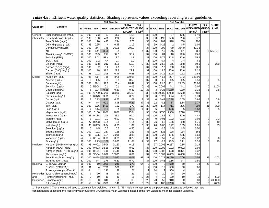
Table 4.8 : Effluent water quality statistics. Shading represents values exceeding receiving water guidelines
N %>DL MIN MAX MEDIANFLOW
WEIGHTED MEAN1
% > GUIDE-LINE2
N %>DL MIN MAX MEDIANFLOW
WEIGHTED MEAN1
% > GUIDE-LINE2
General Suspended Solids (mg/L) 53 100 3.3 67 11.0 18.8 38 100 6 37 13.5 17.9Chemistry Dissolved Solids (mg/L) 53 100 160 486 232 257 38 100 190 506 236 272
Total Solids (mg/L) 53 100 170 495 244 275 38 100 202 528 250 290Oil and grease (mg/L) 50 36 0.25 4 0.95 1.17 36 39 0.25 2 0.5 1.04Conductivity (uS/cm) 52 100 247 748 362.5 397.0 37 100 292 779 364.0 421.8pH 52 100 7.41 8.56 8.1 8.0 4 37 100 7.9 8.45 8.1 8.1 0 6.5-8.5Alkalinity (mg/L CaCO3) 52 100 53.5 217 97.5 96.7 37 100 84 110 98.0 95.0Turbidity (FTU) 53 100 2.01 58.4 8.2 14.8 37 100 5.79 31.8 12.6 15.4BOD (mg/L) 12 100 1.2 4.4 2.7 2.9 5 100 0.4 4 3.4 3.1Chloride (mg/L) 52 100 23.8 212 38.5 53.8 0 37 100 28.2 165 38.8 60.1 0 250Carbon (DOC) (mg/L) 52 100 2 8.2 2.9 3.3 37 100 2.3 7.8 3.0 3.5Carbon (DIC) (mg/L) 52 100 18 31.2 22.8 22.9 37 100 18.8 25.6 22.6 22.2Silicon (mg/L) 52 98 0.02 1.08 0.46 0.53 37 100 0.16 1.08 0.52 0.53
Metals Aluminum (ug/L) 52 98 7.14 736 84.6 130.08 38 100 46.5 297 97.3 129.90Arsenic (ug/L) 52 0 0.5 0.5 0.5 0.50 0 37 0 0.5 0.5 0.5 0.50 0 5Barium (ug/L) 52 100 20.1 39.9 26.4 28.47 38 100 21.3 41.1 27.85 30.06Beryllium (ug/L) 52 0 7E-04 0.1 0.1 0.05 0 38 0 0.009 0.1 0.1 0.07 0 1100Cadmium (ug/L) 52 6 0.04 0.88 0.30 0.37 10 38 3 0.23 0.69 0.30 0.32 5 0.5Calcium (ug/L) 52 100 29700 50200 37000 37753 38 100 29200 45900 37650 37481Chromium (ug/L) 52 6 0.073 3.01 0.7 0.79 38 0 0.322 1.24 0.7 0.74Cobalt (ug/L) 52 2 0.33 5.36 0.65 1.02 2 38 0 0.47 0.98 0.65 0.68 3 0.9Copper (ug/L) 52 94 0.8 52.3 3.95 5.21 37 38 92 0.8 67 3.18 9.77 24 5Iron (ug/L) 52 100 2.76 1450 192 270 17 38 100 114 711 236 304 21 300Lead (ug/L) 52 2 0.14 15.7 5 5.19 4 38 5 5 14.6 5 5.68 5 5Magnesium (ug/L) 52 100 5160 11900 7880 7554 38 100 5550 9980 7720 7675Manganese (ug/L) 52 98 0.134 206 33.3 56.0 38 100 22.2 82.7 31.9 43.7Mercury (ug/L) 37 3 0.01 0.2 0.02 0.02 0 27 0 0.01 0.02 0.02 0.02 0 0.2Molybdenum (ug/L) 52 27 0.223 10.1 0.8 1.14 0 38 26 0.8 9.56 0.8 1.76 0 40Nickel (ug/L) 52 35 0.053 3.84 0.65 1.09 0 38 26 0.65 8.22 0.65 1.01 0 25Selenium (ug/L) 52 0 0.5 0.5 0.5 0.50 37 0 0.5 0.5 0.5 0.50Strontium (ug/L) 52 100 121 237 165 159 38 100 125 198 164 162Titanium (ug/L) 52 98 0.25 13.4 3.095 3.85 38 100 1.28 11.6 4.55 5.63Vanadium (ug/L) 52 2 0.164 3.08 0.75 0.79 0 38 0 0.557 1.4 0.75 0.82 0 6Zinc (ug/L) 52 100 2.23 106 5.855 11.68 2 38 97 0.3 15.5 5.11 6.35 0 20
Nutrients Nitrogen (NH3+NH4) (mg/L) 52 98 0.001 0.506 0.123 0.15 37 97 0.002 0.237 0.15 0.13Nitrogen (NO2) (mg/L) 52 100 0.003 0.528 0.035 0.07 37 100 0.002 0.22 0.032 0.04Nitrogen (NO2+NO3) (mg/L) 52 100 0.121 1.16 0.448 0.47 37 100 0.008 1.28 0.371 0.37Phosphate (mg/L) 52 69 3E-04 0.039 0.0085 0.01 37 62 0.002 0.039 0.008 0.01Total Phosphorus (mg/L) 52 100 0.028 0.156 0.052 0.08 98 37 100 0.028 0.129 0.06 0.08 97 0.03TKN Nitrogen (mg/L) 52 100 0.4 1.76 0.63 0.77 37 100 0.48 2.16 0.7 0.80
Bacteria E. coli (c/100mL)* 11 100 10 9000 240 279 64 7 100 8 650 60 74 29 100F. strep. (c/100mL)* 11 91 4 5700 500 235 7 100 12 500 60 66P. aeruginosa (c/100mL)* 11 64 2 290 28 21 7 14 2 300 4 6
Herbicides 2,4,6 -trichlorophenol (ng/L) 30 7 20 48 20 21 26 4 20 28 20 20and Pentachlorophenol (ng/L) 30 7 10 19 10 11 0 25 4 10 170 10 13 0 500Pesticides Dicamba (ng/L) 30 13 50 340 50 68 0 25 20 50 910 50 89 0 200000
2,4 -D (ng/L) 38 58 100 2300 140 200 0 29 38 100 9700 100 532 3 4000
1. See section 3.7 for the method used to calculate flow weighted means. 2. '% > Guideline' represents the percentage of samples collected that have concentrations exceeding the receiving water guideline. 3.Geometric mean was used instead of the flow weighted mean for bacteria variables.
Category GUIDE-LINE
Cell 3 outlet Cell 5 outlet
Variable

Dunkers Flow Balancing System
Final Report Page 66
In general, Cell 5 effluents were marginally cleaner than those of Cell 3. For example, at cell 5, only 29% of samples had E.coli densities above the provincial guideline, compared to 64% at cell 3. Copper, which is one of the most common road runoff contaminants, was also observed less frequently above the guideline at the cell 5 outlet. These results are not unexpected since the dominant flow path for new event water is through cells 1 to 3 (see mass-based analysis in Appendix D).
4.5.1.2 Sedimentation Cell
As indicated earlier, cell 4 was intended to remove contaminants from water pumped out of cell 1during and after storm events. Water exiting cell 4 subsequently passes through the cell 5 wetland and out to the lake. Table 4.9 shows the cell 4 influent and effluent concentrations for key water quality variables of concern. Only events with paired samples at the inlet and outlet of cell 4 were included. At this location flow proportioning or load based analyses is not required since pumping occurs at a constant rate.1
Table 4.9: Wet weather concentrations for selected water quality variables at the inlet and outlet of cell 4
Cell 4 Inlet Cell 4 Outlet
Min Max Mean Median Min Max Mean Median
TSS (mg/L) 6.0 50.5 19.6 15.5 3.0 35.5 11.1 10.0
TP (mg/L) 0.04 0.20 0.11 0.11 0.03 0.15 0.07 0.06
Copper (ug/L) 2.1 40.0 7.4 7.4 0.8 81.3 6.5 3.7
Zinc (ug/L) 3.4 28.8 16.3 14.5 0.7 24.4 6.3 5.8
E.coli (c./100 mL) 76 30000 2343** 1535 20 17000 275** 380 *n = 29 for TSS, TP, Cu, Zn; n = 6 for E.coli ; ** geomean
Results indicate that cell 4 reduced the concentration of all water quality variables measured in the study. Cell 4 effluent concentrations were similar to those reported for the cell 5 outlet, indicating that pollutant loading into cell 5 from cell 4 was relatively minor and that the wetland does not significantly augment treatment provided by upstream cells. There also appeared to be no significant increase in cell 4 effluent concentrations during large events when the second pump was running, even though the increase in discharge 1 The pump rate varies only when a second pump is triggered by high influent discharge after the cell 4 auto-sampler has begun to collect samples (see section 2.1). This did not occur during any of the events summarized in Table 4.9. Removal efficiencies are not reported because influent concentrations are below the level at which this indicator of performance provides meaningful results (see for example Strecker, 1994).

Dunkers Flow Balancing System
Final Report Page 67
associated with two pumps significantly reduces cell 4 residence time. These results are encouraging since the wetland was partly intended to provide healthy habitat for aquatic organisms and wildlife.
4.5.1.3 Acute toxicity
Large volume samples were collected at the inlet (n = 3) and cell 4 outlet (n = 3) during the 2000 monitoring season to test for acute toxicity to rainbow trout and Daphnia Magna. All samples were found to be non-toxic to test organisms (Table 4.10). Based on these results, toxicity testing was discontinued in 2001 and 2002. Table 4.10: Summary of toxicity results
Inlet Cell 4 outlet Date Rainbow
trout Daphnia Magna
Rainbow trout
Daphnia Magna
September 23/00 -- -- non-lethal non-lethal October 4/00 non-lethal non-lethal non-lethal non-lethal October 27/00 non-lethal non-lethal non-lethal non-lethal November 10/00 non-lethal non-lethal -- -- November 20/00 non-lethal non-lethal -- -- Note: rainbow trout 96 hour acute lethality test; daphnia magna 48 hour acute lethality test
4.5.1.4 Beach impact assessment
One of the reasons that a stormwater facility was built in Bluffers Park was to protect the swimming area approximately half a kilometre east of the facility from high loads of bacteria (Figure 2.1). Historically, the beach has been closed for much of the season because of bacterial contamination. The facility does not appear to have significantly improved this situation, despite significant reductions in E.coli through the facility during rain events (see section 4.7).
To assess the potential impact of effluent E.coli concentrations on beach closings, the geometric mean of five E.coli samples collected at the beach area are compared to effluent event mean concentrations from the facility on the same day (Table 4.11). The data do not suggest any connection between facility effluents and beach concentrations of E.coli. On some occasions, effluent concentrations are high but beach concentrations are low and vice versa. An adverse impact of facility effluent on the beach would likely require much higher concentrations than were observed because of significant dilution in Lake Ontario.

Dunkers Flow Balancing System
Final Report Page 68
Table 4.11: Comparison of facility effluent and Bluffers Park beach E.coli densities.
E.coli Concentrations (coliforms/100 mL)*
Date Cell 3 Cell 5 Bluffers Park Beach
June 13, 2000 3400 blocked (no flow) 1105
June 15, 2000 80** blocked (no flow) 777
July 17, 2000 9000 blocked (no flow) 50++
August 8, 2000 700 blocked (no flow) 580++
September 11, 2000 4000** 650 762
October 4, 2000 10 n/a 11
June 11, 2001 180 n/a 1238
June 20, 2001 16 60 434
July 17, 2001 1400 620 3365
August 16, 2001 n/a 50 80
October 16, 2001 80 60 1086
Provincial guideline for body contact recreation is 100 coliforms/100 mL *Dunkers samples are 24 bottle composites collected over 4 hours; Bluffers Park beach sample concentrations represent the geometric mean of 5 grab samples collected along the shore of the beach. **Grab samples collected from Lake Ontario immediately downstream of the facility had E.coli concentrations of 80 and 72 c./100 mL on June 15th and September 11th , respectively. ++The storm occurred late in the day. Beach samples were collected the following morning.
4.5.2 Post Event Sampling
Sampling after runoff events (hereafter referred to as ‘post event sampling’) was conducted for selected events in 2001 to determine changes in effluent water quality as runoff stored from a previous event was pumped continuously into cell 4, through cell 5 and out to the lake. Complete pump-out of water in cells 1, 2 and 3 requires roughly 120 hours; or 60 hours with both cell 4 pumps running. Automated ‘post event samplers’ were stationed next to event samplers at the cell 4 inlet and cell 5 outlet and were programmed with an 8 hour delay (representing the event duration) to collect 24 discrete samples over a period of 24 and 48 hours respectively. The discrete samples were subsequently divided into 3 composites, representing 8 hour time intervals at cell 4 and 16 hour time intervals at cell 5.

Dunkers Flow Balancing System
Final Report Page 69
Table 4.12 presents the results of event and post event sampling for two mid-sized events and two large events. The event sample composites were collected during the runoff event (8 hour duration). The post event samples at the cell 4 inlet and cell 5 outlet were collected after the end of runoff over 3 consecutive 8 and 16 hour time periods, respectively. The second pump at cell 1 was triggered during the August 26th and September 21st events, causing a doubling of the rate at which water was transferred from cell 1 to cell 4. All events show a gradual decline in suspended solids over time to a background concentration consisting primarily of very fine particles of between 8 and 12 mg/L. Concentrations of other constituents that are strongly adsorbed by suspended solids, such as phosphorus, copper and zinc, displayed a more significant reduction at the cell 4 station. The same is true for oil and grease, which was below detection levels at cell 5. These results demonstrate the water quality benefit associated with incremental increases in the settling period, as well as the concentration limits (sometimes referred to as ‘irreducible concentrations’) beyond which further reductions are either impossible or very slow (given a fixed baseflow rate and in-pond sources of these pollutants). 4.5.3 Dry Weather Concentrations
Table 4.13 summarizes average event mean concentrations (AEMCs) and detection frequencies at the inlet and outlet during dry weather. Under dry-weather conditions, the influent is storm sewer baseflow that consists primarily of groundwater that has infiltrated into the pipes through cracks and fissures; it contains little suspended material but can contain somewhat elevated concentrations of constituents related to alkalinity, salinity and soluble metals. The storage and treatment cells contain residual suspended material from previous runoff events. The suspended material in the wetland (cell 5) may also originate from algae growth and sediment resuspension induced by wind, fish or waterfowl.
During dry weather, outlet AEMC detection frequencies below 20% were noted for arsenic, beryllium, cadmium, chromium, cobalt, lead, mercury, selenium vanadium, 2-4-6 trichlorophenol, dicamba, 2-4-D and several other organic parameters not included in Table 4.13, but listed in Appendix F. Suspended solids displayed a slight increase through the pond, while other common stormwater contaminants, including zinc, copper, phosphorus and bacteria showed significant reductions. Chloride was reduced because it is denser than water and tends to concentrate at the bottom of stormwater ponds during dry periods (i.e. it shows net removal); this constituent is flushed from the facility during large storm events.
Despite these reductions, average concentrations of total phosphorus, iron and E.coli exceeded PWQOs (MOEE, 1994) at one or both of the two outlets. All lake water pollutant concentrations were consistently less than their respective PWQO values.

Table 4.12 : Event and post event composite samples for selected water quality variables
Event EventHours from start of runoff 0 - 8 hrs 8 - 16 hrs 16 - 24 hrs 24 - 32 hrs 0 - 8 hrs 8 - 24 hrs 24 - 40 hrs 40 - 56 hrsAug 19/01 (rain = 9.2 mm)TSS (m/L) 25.5 18.0 13.5 11.5 19.5 16.0 14.0 12.5Total Solids (mg/L) 236 214 210 218 256 250 242 240TDS (mg/L) 212 196 196 206 236 232 228 228Oil and Grease (mg/L) 1.2 1.4 1.4 1.2 <dl <dl <dl <dlTotal Phosphorus (mg/L) 0.11 0.09 0.08 0.07 0.07 0.06 0.06 0.06TKN (mg/L) 0.82 0.76 0.72 0.72 0.80 0.72 0.76 0.72Copper (ug/L) 6.8 6.5 5.1 4.1 4.1 2.7 3.0 2.5Iron (ug/L) 419 427 295 264 310 246 236 186Zinc (ug/L) 19.6 17.2 14.0 9.1 7.0 6.9 6.3 5.3
Aug 26/01 (rain = 11.2 mm)TSS (m/L) 50.5 29.0 18.0 8.5 16.0 12.5 11.0 10.0Total Solids (mg/L) 266 232 218 320 238 238 232 230TDS (mg/L) 216 202 200 312 220 226 220 220Oil and Grease (mg/L) 1.4 n/a n/a n/a <dl n/a n/a n/aTotal Phosphorus (mg/L) 0.17 0.17 0.12 0.07 0.08 0.06 0.08 0.07TKN (mg/L) 1.20 1.04 0.92 0.76 0.80 0.68 0.80 0.68Copper (ug/L) 7.5 6.5 4.6 2.8 2.5 2.1 2.5 2.6Iron (ug/L) 367 213 158 87 121 92 98 97Zinc (ug/L) 27.6 20.2 12.4 6.6 5.6 4.1 4.8 3.9
Sep 19/01 (rain = 24.4 mm)TSS (m/L) 16.5 13.5 10.0 8.5 24.5 17.0 14.5 10.5Total Solids (mg/L) 172 160 164 178 250 240 228 224TDS (mg/L) 156 146 156 170 226 224 214 212Oil and Grease (mg/L) 1.0 1.4 1.4 1.2 <dl <dl <dl <dlTotal Phosphorus (mg/L) 0.11 0.10 0.08 0.07 0.06 0.06 0.07 0.05TKN (mg/L) 0.72 0.72 0.68 0.68 0.76 0.64 0.68 0.64Copper (ug/L) 9.1 7.6 5.9 5.1 3.0 2.4 2.6 2.3Iron (ug/L) 275 238 197 188 284 265 263 168Zinc (ug/L) 21.5 17.9 12.8 12.9 4.5 5.4 6.1 4.4
Sep 21/01 (rain = 22.4 mm)TSS (m/L) 23.0 20.0 19.0 15.5 n/a 14.5 13.5 8.0Total Solids (mg/L) 172 154 156 166 n/a 210 198 180TDS (mg/L) 148 134 136 152 n/a 196 184 172Oil and Grease (mg/L) 1.8 1.6 1.5 1.4 n/a <dl <dl <dlTotal Phosphorus (mg/L) 0.11 0.10 0.09 0.08 n/a 0.08 0.07 0.05TKN (mg/L) 0.80 0.76 0.76 0.78 n/a 0.76 0.72 0.64Copper (ug/L) 7.2 7.0 5.7 4.9 n/a 3.4 2.6 2.6Iron (ug/L) 340 332 296 244 n/a 254 221 165Zinc (ug/L) 24.7 23.4 18.4 13.2 n/a 8.1 7.2 6.6
* Cell 4 and 5 event composites were collected over 8 hours. Cell 4 and 5 post event samples were collected over 24 and 48 hour periods. Each post event composite sample represents a period of 8 and 16 hours, respectively.
Cell 4 Inlet Composite Samples Cell 5 Outlet Composite SamplesPost Event Post Event

Table 4.13 : Dry weather median concentrations and detection frequencies GUIDE-
Category Variable RMDL %>RMDL MEDIAN %>RMDL MEDIAN %>RMDL MEDIAN %>RMDL MEDIAN %>RMDL MEDIAN LINEGeneral Suspended Solids (mg/L) 2.5 46 2.5 100 11.25 93 8 100 11 29 1.25Chemistry Dissolved Solids (mg/L) 10 100 913 100 226 100 254 100 294 100 192
Total Solids (mg/L) 10 100 918 100 239 100 266 100 308 100 196Oil and Grease (mg/L) 1 41 1 30 0.5 27 0.5 35 0.5 21 0.5Conductivity (uS/cm) 1 100 1505 100 348.5 100 391 100 453 100 296pH 0.1 100 8.2 100 8.1 100 8.2 100 8.2 100 8.3Alkalinity (mg/L CaCO3) 2.5 100 219.5 100 98.25 100 97 100 107 100 92Turbidity (FTU) 0.01 100 2.1 100 10 100 7.1 100 11.5 100 0.78BOD (mg/L) 0.2 89 2.2 100 2.8 100 2.2 100 3 100 0.7Chloride (mg/L) 0.2 100 315 100 36.6 100 52.8 100 56.8 100 21.8 250Carbon (DOC) (mg/L) 0.1 100 3.5 100 3 100 3.4 100 3.4 100 1.9Carbon (DIC) (mg/L) 0.2 100 51.4 100 22.3 100 23.2 100 24.6 100 21.6Silicon (mg/L) 0.02 100 4.02 100 0.38 100 0.7 100 0.6 100 0.13
Metals Aluminum (ug/L) 11 100 64.05 100 77.5 100 64.1 100 102 71 19.1Arsenic (ug/L) 1 0 0.5 0 0.5 0 0.5 0 0.5 0 0.5 0.1Barium (ug/L) 0.2 100 57.95 100 26.4 100 26.7 100 31.1 100 21.35Beryllium (ug/L) 0.2 0 0.1 0 0.1 0 0.1 0 0.1 0 0.1 1100Cadmium (ug/L) 0.6 14 0.3 0 0.3 0 0.3 4 0.3 0 0.3 0.5Calcium (ug/L) 5 100 112500 100 36900 100 36400 100 42300 100 33500Chromium (ug/L) 1.4 25 0.7 0 0.7 19 0.7 22 0.7 14 0.7Cobalt (ug/L) 1.3 4 0.65 0 0.65 0 0.65 0 0.65 0 0.65 0.9Copper (ug/L) 1.6 100 8.87 60 1.74 70 3.41 78 2.82 36 0.8 5Iron (ug/L) 0.8 100 100.6 100 182.5 100 126 100 216 100 29.6 300Lead (ug/L) 10 4 5 0 5 4 5 0 5 7 5 5Magnesium (ug/L) 8 100 16650 100 7790 100 8130 100 8640 100 8455Manganese (ug/L) 0.2 100 18.6 100 37.5 100 44.9 100 49.5 100 2.315Mercury (ug/L) 0.02 4 0.02 0 0.02 0 0.02 0 0.02 0 0.02 0.2Molybdenum (ug/L) 1.6 46 0.8 30 0.8 56 1.69 52 1.65 7 0.8 40Nickel (ug/L) 1.3 36 0.65 30 0.65 48 0.65 39 0.65 21 0.65 25Selenium (ug/L) 1 0 0.5 0 0.5 0 0.5 0 0.5 0 0.5Strontium (ug/L) 0.1 100 347 100 162 100 166 100 181 100 160.5Titanium (ug/L) 0.5 43 0.25 100 2.515 89 1.89 100 3.97 43 0.25Vanadium (ug/L) 1.5 4 0.75 0 0.75 4 0.75 0 0.75 0 0.75 6Zinc (ug/L) 0.6 100 16.3 100 5.65 100 6.17 100 7.58 79 1.0285 20
Nutrients Nitrogen (NH3+NH4) (mg/L) 0.002 93 0.109 100 0.136 93 0.128 96 0.098 86 0.03Nitrogen (NO2) (mg/L) 0.001 100 0.064 100 0.035 100 0.037 100 0.034 100 0.012Nitrogen (NO2+NO3) (mg/L) 0.005 100 2.725 100 0.3555 100 0.364 100 0.437 100 0.362Phosphate (mg/L) 0.005 96 0.076 50 0.006 48 0.005 43 0.0025 7 0.0025Total Phosphorus (mg/L) 0.002 100 0.127 100 0.053 100 0.054 100 0.06 100 0.012 0.03TKN Nitrogen (mg/L) 0.02 100 0.64 100 0.65 100 0.68 100 0.72 100 0.27
Bacteria E. coli (c/100mL) 4 100 1400 100 140 100 50 100 70 100 42 100F. streptococcus (c/100mL) 4 100 2050 100 50 100 50 100 25 70 40P. aeruginosa (c/100mL) 4 100 70 37.5 4 29 4 17 4 10 4
Herbicides & 2,4,6 -trichlorophenol (ng/L) 20 11 20 0 20 11 20 5 20 11 20Pesticides Pentachlorophenol (ng/L) 10 11 10 0 10 22 10 17 10 0 10 500
Dicamba (ng/L) 50 33 50 25 50 22 50 39 50 0 50 2E+052,4 -D (ng/L) 100 39 100 25 11.25 59 205 53 11 13 100 4000
PAHs none detected
Note: see Appendix F for detailed dry weather statistics.
Lake OntarioInlet Cell 4 inlet Cell 3 Outlet Cell 5 Outlet

Dunkers Flow Balancing System
Final Report Page 72
4.5.4 Water Temperature
Table 4.14 compares the average, minimum, maximum and frequency above 21°C at each monitoring station for the 2000 to 2002 monitoring seasons. The generally accepted limit for cold water fisheries habitat is 21°C. Graphs of continuous temperature data are provided in Appendix G. As indicated earlier, the 2002 temperature measurements were taken at three depths on the cell 2 side of the cell 1-2 pontoon.
These temperature data indicate an average temperature rise of between 7.1 and 8.7°C as water passes through the facility. The maximum temperature observed at the inlet was 25°C, compared to 29°C at the outlets. Only rarely did inlet temperatures rise above 21°C, whereas outlet temperatures were frequently above the threshold. Fortunately, warm water discharges from the facility do not affect the lake in the way they would affect small streams, and are therefore not a concern from a receiving water protection perspective. These discharges do, however, influence the type and diversity of aquatic species that may find their way into the wetland.
The temperature depth profile conducted in 2002 indicates a difference in maximum temperature measured at the surface (0.5 m) and that measured at 1.5 and 2.5 m depths of 5.0 and 6.4°C, respectively. During especially warm periods, the temperature differential between the surface and bottom temperatures increases to as much as 9°C.
Water temperature in the facility responded primarily to diurnal fluctuations in air temperature and solar radiation. Inlet water temperatures, by contrast, fluctuated mostly in response to surface runoff during rain events.
Table 4.14: Water temperature statistics
Monitoring station
Average °C
Minimum °C
Maximum °C
Frequency above 21°C (%)
July 13 – August 9, 2000+ Inlet 15.5 13.4 25.0 1 Cell 3 22.6 18.7 28.6 78 Cell 5 23.0 18.7 29.4 85 June 12 – August 31, 2001+ Inlet 14.1 11.8 23.5 0.1 Cell 4 inlet 21.8 16.5 27.8 65 Cell 5 22.8 17.4 28.9 77 June 6 – August 31, 2002* Cell 2 (0.5 m) 24.5 15.6 31.5 88 Cell 2 (1.5 m) 22.4 15.6 26.5 77 Cell 2 (2.5 m) 20.9 14.1 25.1 68 +Temperature measurements in 2000 and 2001 were taken 0.5 m below the water surface at locations shown in Figure 2.3. *Measurements in cell 2 were taken off the cell 1-2 pontoon and represent depths below the water surface. During wet weather, the pontoon and measurement locations float up and down as water levels in the facility fluctuate.

Dunkers Flow Balancing System
Final Report Page 73
4.6 Sediment Quality The quality and particle size distribution of bottom sediments were determined in order to characterize the location and relative magnitude of contaminant deposition within each of the cells, and to assess potential impacts of effluent discharges on receiving waters. Figure 4.23 shows the location of sediment sampling conducted on November 16, 2001.
4.6.1 Sediment Chemistry
Table 4.15 presents the mean sediment chemistry data at each sampling location and compares these to provincial sediment quality guidelines. Sediment chemistry within the facility are not required or expected to meet these guidelines; they are provided only as a standard of comparison. All of the sediment chemistry data are presented in Appendix H.
Sediment chemistry results show that quality generally improves as distance from the inlet increases, which is consistent with characterizations of the depositional environment reported in section 4.4. Although water is continuously transferred directly from cell 1 to cell 4, the latter cell has considerably cleaner sediment and lower organic carbon levels. The exception is oil and grease (solvent extractable), which had much higher levels in cell 4. Oil and grease, unlike most other contaminants reported, is lighter than water and therefore may remain in the water column longer after a storm where it is more susceptible than other contaminants to capture by the cell 1 pump. Sample A, collected closest to the cell 4 pump outfall, had much higher levels of oil and grease and other contaminants relative to downstream samples (see Appendix H). Individual samples at cell 3 showed a similar pattern to that of cell 4, with poorer sediment quality in samples A and B relative to sample C, indicating that most contaminants were removed in the upstream portions of cell 3. Cell 5 had the lowest sediment contaminant levels and can be considered suitable for aquatic habitat based on Provincial Sediment Quality Guidelines for Aquatic Life (MOE, 1993). Interestingly, among individual cell 5 sediment samples, sample C, collected closest to the outlet, had marginally higher contaminant levels than samples B and A. Dye test results indicated that flow is short circuiting through cell 5 along the west side of the island, which may explain the slightly higher contaminant levels in sample C. Extending the cobblestone spit located downstream of the cell 4 outlet (Figure 4.23) would help to improve residence time by diverting flow around the east side of the island. Lake Ontario sediments were collected immediately downstream of the facility outfalls and on the south side of the embayment (control) (Figure 4.23). As expected, the Lake Ontario sediment samples were substantially cleaner than the facility sediments. Relative to the Lake Ontario outfall site, the control had less copper, similar levels of zinc, lead and nutrients, and higher levels of PCBs, iron and oil and grease. Lake sediments are highly mobile and thus the relatively clean sediments at the Lake Ontario outfall station should not be

Sediment Pond
Mud Flat
Sediment Pond
OutletStructure
OutletStructure
Fence
Fence
Water Pumped from Lake Ontario
Sewer Outfall Structureand Inlet Weir
Stilling Well
Ils and
Lake Ontario
Lake Ontario
PumpStation
CELL 4
CELL 1
CELL 5WETLAND
CELL 3
CELL 2
Lake OntarioControl
A
B
C
C
B
A
A
BC
A
BC
A
B
C
Sediment Sampling Sites
Figure 4.23: Sediment sampling sites
A B C

Table 4.15: Mean sediment chemistry results, provincial sediment quality guidelines (PSQG) and soil background concentrations in Ontario
Lake Ont. Background Conc.Group Variable Units C ell 1 Cell 3 Cell4 Cell 5 Lake Ontario Control LEL SEL** Agr. Non Agr.General Chemistry Carbon; total organic mg/g dry 30.0 31.7 21.0 5.3 1.7 2.0 1% 10%
Total Solids; loss on ignition mg/g dry 57.0 58.7 49.0 10.4 6.2 4.2Oil and grease mg/L 8600 6000 18800 420 113 217
Metals Mercury ug/g dry 0.16 0.04 0.02 0.01 0.01 0.01 0.20 2.00 0.16 0.23Beryllium ug/g dry 0.5 0.7 0.6 0.5 0.5 0.5 1.2 1.2Magnesium ug/g dry 14667 12200 13000 5533 3767 3833Aluminum ug/g dry 12000 14933 16333 4700 3567 2500Calcium ug/g dry 96333 88333 87000 44333 43667 57000Vanadium ug/g dry 35.3 38.7 41.7 18.0 13.0 18.7 91 91Chromium ug/g dry 39.3 34.7 36.7 10.3 7.3 7.0 26 110 67 71Manganese ug/g dry 453 460 503 217 170 183 460 1100Iron ug/g dry 19333 14267 24000 9333 6467 8000 2% 4%Cobalt ug/g dry 8.1 9.2 10.2 4.1 2.9 2.7 19 21Nickel ug/g dry 21.3 24.3 25.7 8.6 6.4 4.5 16 75 43 43Copper ug/g dry 66.0 49.7 46.7 9.0 5.7 1.3 16 110 56 85Zinc ug/g dry 233.3 166.3 156.7 29.0 12.0 13.0 120 820 150 160Molybdenum ug/g dry 0.7 0.7 0.5 0.6 0.5 0.5 2.5 2.5Cadmium ug/g dry 1.3 1.1 1.0 0.4 0.4 0.3 0.60 10.00 1 1Barium ug/g dry 78.3 82.0 89.0 19.3 11.7 8.3 190 210Lead ug/g dry 53.0 35.7 36.3 7.7 4.3 5.3 31 250 55 120Strontium ug/g dry 146.7 139.7 136.7 75.3 78.0 84.0Titanium ug/g dry 643 690 743 460 357 590Arsenic ug/g dry 3.3 4.2 4.3 1.4 1.0 1.4 6.0 33.0 14 17Selenium ug/g dry 0.3 0.5 0.4 0.2 0.2 0.2
Nutrients Nitrogen; total Kjeldahl mg/g dry 1.7 2.2 1.6 0.6 0.2 0.2 0.55 4.80Phosphorus; total mg/g dry 0.81 0.83 0.78 0.51 0.48 0.49 0.60 2.00
PCBs and OC PCB; total ng/g dry 60.0 73.3 66.7 33.3 20.0 33.3 70 15900 300 300Pesticides* Hexachlorobenzene ng/g dry 1.3 1.0 1.3 1.0 1.0 1.0 20 720
pp-DDE ng/g dry 5.7 3.3 3.7 1.0 1.0 1.0 5 570PAHs Naphthalene ng/g dry 20 20 20 20 20 20 50 90
Acenaphthylene ng/g dry 33 20 20 20 20 20 80 80Acenaphthene ng/g dry 40 20 20 20 20 20 50 70Flourene ng/g dry 100 20 20 20 20 20 190 4800 50 120Phenanthrene ng/g dry 1567 273 200 73 20 20 560 28500 190 690Anthracene ng/g dry 173 33 20 20 20 20 220 11100 50 160Flouranthene ng/g dry 3600 713 633 113 20 20 750 30600 240 1100Pyrene ng/g dry 2767 553 480 100 20 20 490 25500 190 1000Benzo(a)anthracene ng/g dry 1113 207 173 47 20 20 320 44400 100 740Chrysene ng/g dry 1833 413 360 67 20 20 340 13800 180 690Benzo(b)fluoranthene ng/g dry 2267 527 480 73 20 20 300 470Benzo(k)fluoranthene ng/g dry 787 180 160 27 20 20 240 40200 50 480Benzo(a)pyrene ng/g dry 1233 253 227 53 40 40 370 43200 100 490Indeno(1,2,3-c,d)pyrene ng/g dry 1247 320 307 53 40 40 200 9600 110 380Dibenzo(a,h)anthracene ng/g dry 253 67 40 40 40 40 60 3900 150 160Benzo(g,h,i)perylene ng/g dry 993 267 240 40 40 40 170 9600 200 680d8-naphthalene %R 40 46 46 59 70 62d10-phenanthrene %R 95 91 89 90 97 103d12-chrysene %R 69 70 69 84 81 85
*none of the other 32 pesticides/herbicides analyzed were detected above laboratory analytical detection limits** SEL values for PAHs and PCBs/Organochlorine Pesticides are converted to bulk sediment values based on a total organic carbon content of 3%.
PSQGMean Concentrations (n=3)
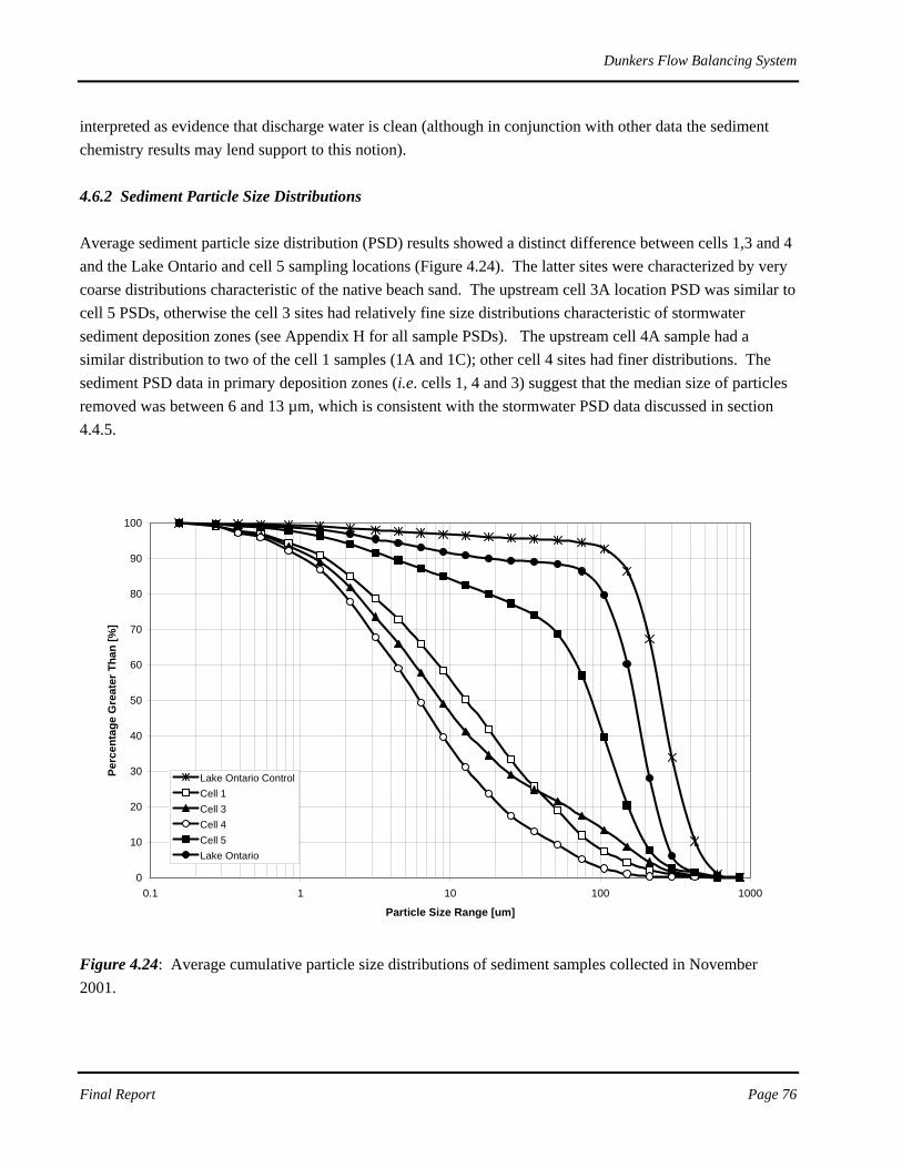
Dunkers Flow Balancing System
Final Report Page 76
interpreted as evidence that discharge water is clean (although in conjunction with other data the sediment chemistry results may lend support to this notion). 4.6.2 Sediment Particle Size Distributions Average sediment particle size distribution (PSD) results showed a distinct difference between cells 1,3 and 4 and the Lake Ontario and cell 5 sampling locations (Figure 4.24). The latter sites were characterized by very coarse distributions characteristic of the native beach sand. The upstream cell 3A location PSD was similar to cell 5 PSDs, otherwise the cell 3 sites had relatively fine size distributions characteristic of stormwater sediment deposition zones (see Appendix H for all sample PSDs). The upstream cell 4A sample had a similar distribution to two of the cell 1 samples (1A and 1C); other cell 4 sites had finer distributions. The sediment PSD data in primary deposition zones (i.e. cells 1, 4 and 3) suggest that the median size of particles removed was between 6 and 13 µm, which is consistent with the stormwater PSD data discussed in section 4.4.5.
0
10
20
30
40
50
60
70
80
90
100
0.1 1 10 100 1000
Particle Size Range [um]
Perc
enta
ge G
reat
er T
han
[%]
Lake Ontario ControlCell 1Cell 3Cell 4Cell 5Lake Ontario
Figure 4.24: Average cumulative particle size distributions of sediment samples collected in November 2001.
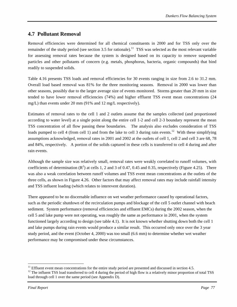
Dunkers Flow Balancing System
Final Report Page 77
4.7 Pollutant Removal
Removal efficiencies were determined for all chemical constituents in 2000 and for TSS only over the remainder of the study period (see section 3.5 for rationale).11 TSS was selected as the most relevant variable for assessing removal rates because the system is designed based on its capacity to remove suspended particles and other pollutants of concern (e.g. metals, phosphorus, bacteria, organic compounds) that bind readily to suspended solids.
Table 4.16 presents TSS loads and removal efficiencies for 30 events ranging in size from 2.6 to 31.2 mm. Overall load based removal was 81% for the three monitoring seasons. Removal in 2000 was lower than other seasons, possibly due to the larger average size of events monitored. Storms greater than 20 mm in size tended to have lower removal efficiencies (74%) and higher effluent TSS event mean concentrations (24 mg/L) than events under 20 mm (91% and 12 mg/L respectively).
Estimates of removal rates to the cell 1 and 2 outlets assume that the samples collected (and proportioned according to water level) at a single point along the entire cell 1-2 and cell 2-3 boundary represent the mean TSS concentration of all flow passing these boundaries. The analysis also excludes consideration of TSS loads pumped to cell 4 (from cell 1) and from the lake to cell 3 during rain events.12 With these simplifying assumptions acknowledged, removal rates in 2001 and 2002 at the outlets of cell 1, cell 2 and cell 3 are 68, 78 and 84%, respectively. A portion of the solids captured in these cells is transferred to cell 4 during and after rain events.
Although the sample size was relatively small, removal rates were weakly correlated to runoff volumes, with coefficients of determination (R2) at cells 1, 2 and 3 of 0.47, 0.45 and 0.35, respectively (Figure 4.25). There was also a weak correlation between runoff volumes and TSS event mean concentrations at the outlets of the three cells, as shown in Figure 4.26. Other factors that may affect removal rates may include rainfall intensity and TSS influent loading (which relates to interevent duration).
There appeared to be no discernable influence on wet weather performance caused by operational factors, such as the periodic shutdown of the recirculation pumps and blockage of the cell 5 outlet channel with beach sediment. System performance (removal efficiencies and effluent EMCs) during the 2002 season, when the cell 5 and lake pump were not operating, was roughly the same as performance in 2001, when the system functioned largely according to design (see table 4.1). It is not known whether shutting down both the cell 1 and lake pumps during rain events would produce a similar result. This occurred only once over the 3 year study period, and the event (October 4, 2000) was too small (6.6 mm) to determine whether wet weather performance may be compromised under these circumstances.
11 Effluent event mean concentrations for the entire study period are presented and discussed in section 4.5. 12 The influent TSS load transferred to cell 4 during the period of high flow is a relatively minor proportion of total TSS load through cell 1 over the same period (see Appendix D).

Table 4.16 : TSS loads and removal efficiencies
Event Flow TSS Removal Efficiency (%)Date Total (mm) Duration (h) Volume (m3) Inlet Cell 1 Cell 2 Outlet** Inlet Cell 1* Cell 2* Outlet** Cell 1 Cell 2 Outlet
14-Jul-00 20.9 3.1 19342 230.0 n/a n/a 29.0 4448.7 n/a n/a 560.9 n/a n/a 87.417-Jul-00 31.2 1.3 29148 117.0 n/a n/a 67.0 3410.3 n/a n/a 1952.9 n/a n/a 42.730-Jul-00 30.2 3.4 18987 134.0 n/a n/a 23.5 2544.3 n/a n/a 446.2 n/a n/a 82.58-Aug-00 19.4 7 11993 341.0 n/a n/a 20.5 4089.6 n/a n/a 245.9 n/a n/a 94.023-Aug-00 23.2 7.5 12166 120.0 n/a n/a 17.5 1459.9 n/a n/a 212.9 n/a n/a 85.42-Sep-00 5.5 6.9 2551 268.0 n/a n/a 14.0 683.7 n/a n/a 35.7 n/a n/a 94.810-Sep-00 18 2.8 10555 79.0 n/a n/a 13.8 833.8 n/a n/a 145.1 n/a n/a 82.614-Sep-00 22 7.5 10263 38.5 n/a n/a 15.5 395.1 n/a n/a 159.1 n/a n/a 59.723-Sep-00 5.8 0.3 3346 63.5 n/a n/a 12.8 212.5 n/a n/a 42.7 n/a n/a 79.94-Oct-00 6.6 5.4 2500 97.5 n/a n/a 6.5 243.8 n/a n/a 16.3 n/a n/a 93.327-Oct-00 2.6 2.6 1034 74.5 n/a n/a 10.0 77.0 n/a n/a 10.3 n/a n/a 86.63-Jun-01 5.2 1.1 2376 61.6 14.5 14.5 18.0 146.4 34.5 34.5 42.8 76.5 76.5 70.811-Jun-01 18.2 8.9 8555 71.9 25.3 12.6 8.7 615.1 216.4 107.8 74.4 64.8 82.5 87.920-Jun-01 4.1 5.2 1344 86.6 7.0 8.0 14.4 116.4 9.4 10.8 19.4 91.9 90.8 83.430-Jun-01 5.6 0.8 2041 155.9 n/a n/a 6.6 318.2 n/a n/a 13.5 n/a n/a 95.817-Jul-01 12.4 7.5 4646 68.9 8.0 13.5 9.4 320.1 37.2 62.7 43.6 88.4 80.4 86.419-Aug-01 9.8 6.1 6035 51.0 12.5 n/a 10.5 307.8 75.4 n/a 63.4 75.5 n/a 79.426-Aug-01 7 3.1 5202 251.0 36.3 19.5 10.8 1305.7 188.8 101.4 55.9 85.5 92.2 95.719-Sep-01 24.4 11.5 15520 43.5 14.3 8.9 11.8 675.1 221.9 138.1 183.1 67.1 79.5 72.921-Sep-01 22.4 8.6 14030 58.4 20.5 13.2 10.4 819.4 287.6 185.2 145.9 64.9 77.4 82.211-Oct-01 19.2 15.9 9878 31.5 n/a 6.5 11.3 311.2 n/a 64.2 111.1 n/a 79.4 64.316-Oct-01 8.6 3.9 4890 52.1 26.4 14.5 10.2 254.8 129.1 70.9 49.9 49.3 72.2 80.423-Oct-01 6.2 1.3 3255 115.7 27.2 15.3 7.6 376.6 88.5 49.8 24.8 76.5 86.8 93.425-Nov-01 25.2 5.6 15000 79.7 52.9 33.0 14.7 1195.5 793.5 495.0 220.5 33.6 58.6 81.631-May-02 6.8 1.8 3577 131.7 32.8 n/a 13.5 471.1 117.3 n/a 48.3 75.1 n/a 89.721-Jun-02 12.7 4 5704 197.4 28.0 9.5 9.2 1126.0 159.7 54.2 52.5 85.8 95.2 95.39-Jul-02 5 2.8 2157 188.0 12.0 8.7 10.2 405.5 25.9 18.8 22.0 93.6 95.4 94.621-Jul-02 25.7 2.4 12338 104.3 34.6 32.4 28.8 1286.9 426.9 399.8 355.3 66.8 68.9 72.422-Jul-02 23.3 3.8 12603 92.8 62.7 39.9 18.3 1169.6 790.2 502.9 230.6 32.4 57.0 80.322-Aug-02 7.5 1.6 3850 107.5 10.0 11.0 14.0 413.9 38.5 42.4 53.9 90.7 89.8 87.0Summary Mean2000 16.9 4.3 11080 142.1 n/a n/a 20.9 18398.7 n/a n/a 3828.0 n/a n/a 79.22001 12.9 6.1 7136 86.8 22.3 14.5 11.1 6762.1 2082.4 1320.4 1048.3 66.0 78.5 84.52002 13.5 2.7 6705 137.0 30.0 20.3 15.7 4872.9 1558.5 1017.9 762.6 68.0 76.9 84.32001 and 2002 13.1 5.0 7000 102.6 25.0 16.3 12.5 11635.0 3640.9 2338.3 1810.9 67.8 77.8 84.4events >20 mm 24.9 5.5 15939.7 101.8 37.0 25.5 23.7 17404.7 n/a n/a 4467.5 n/a n/a 74.3events < 20mm 9.3 4.5 4774.5 124.7 20.0 12.1 11.6 12629.0 n/a n/a 1171.4 n/a n/a 90.7all events 14.5 4.8 8496 117.1 25.0 16.3 15.6 30033.7 n/a n/a 5638.9 n/a n/a 81.2
** Outlet values represent a weighted average of the cell 3 and cell 5 outets, as discussed in section 3.7. During the 10 events when cell 5 was blocked with beach sediment all flow was assumed to exit through cell 3.
*Loads at cell 1 and 2 are calculated based on total inflow volumes and do not consider volumes pumped to cell 4 during the event. Note: See section 3.5 for details on how Event Mean Concentrations were determined.
TSS Concentration (mg/L)Precipitation TSS Load (kg)
Load-based TotalTotalMeanMean
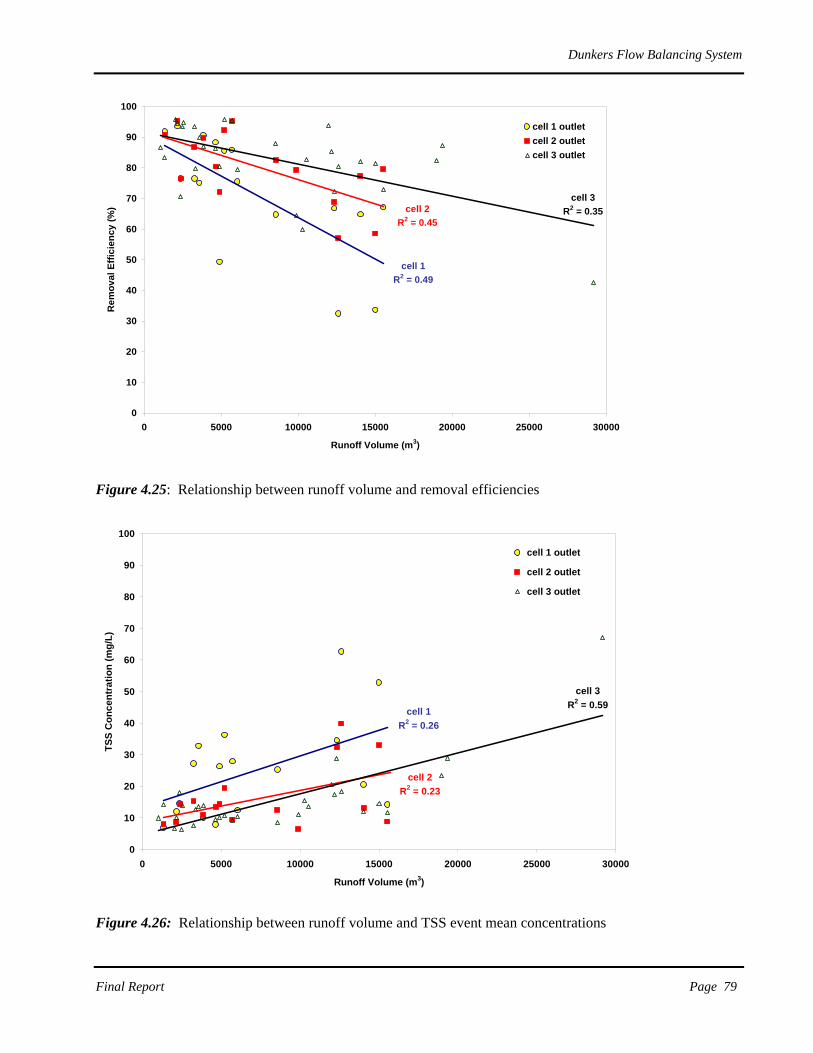
Dunkers Flow Balancing System
Final Report Page 79
cell 3R2 = 0.35
cell 1R2 = 0.49
cell 2R2 = 0.45
0
10
20
30
40
50
60
70
80
90
100
0 5000 10000 15000 20000 25000 30000
Runoff Volume (m3)
Rem
oval
Effi
cien
cy (%
)cell 1 outletcell 2 outletcell 3 outlet
Figure 4.25: Relationship between runoff volume and removal efficiencies
cell 1R2 = 0.26
cell 2R2 = 0.23
cell 3R2 = 0.59
0
10
20
30
40
50
60
70
80
90
100
0 5000 10000 15000 20000 25000 30000
Runoff Volume (m3)
TSS
Con
cent
ratio
n (m
g/L)
cell 1 outlet
cell 2 outlet
cell 3 outlet
Figure 4.26: Relationship between runoff volume and TSS event mean concentrations

Dunkers Flow Balancing System
Final Report Page 80
Figure 4.27 presents removal efficiencies for all water quality variables based on 11 events monitored in 2000. These results indicate overall removal of 79% for TSS, 77% for total phosphorus, and 75% for E.coli (n = 4).
Performance for most metals exceeded 70%, except magnesium and calcium, which would not necessarily be expected to decline, and trace metals that had very low inlet concentrations (e.g. titanium, barium, arsenic, cobalt, molybdenum). Cadmium is one of the few heavy metals that is found mostly in dissolved form. Hence, BMPs such as the Dunkers FBS that rely on sedimentation for treatment are often not effective in removing this constituent. Effluent concentrations for this metal did not exceed receiving water guidelines.
Negative removal rates were rare but can occur if the effluent concentration of a particular constituent is greater than its respective influent concentration due to in-facility sources of contaminants that are either present naturally in native soils or were deposited during dry weather (or previous events). These negative removal rates are only a concern if effluent concentrations are elevated above guideline levels, which was not the case in the Dunkers facility.
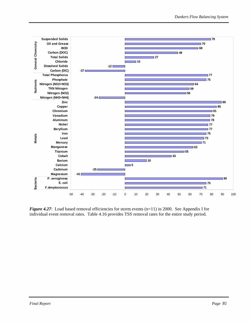
Dunkers Flow Balancing System
Final Report Page 81
7175
90-41
-255
2043
5563
7173
757777
7879
8185
89-24
5659
647577
-37-12
1027
4968
7079
-50 -40 -30 -20 -10 0 10 20 30 40 50 60 70 80 90 100
F.streptococcus E. coli
P. aeruginosa Magnesium
Cadmium Calcium Barium Cobalt
Titanium Manganese
Mercury Lead Iron
Beryllium Nickel
Aluminum Vanadium Chromium
Copper Zinc
Nitrogen (NH3+NH4)Nitrogen (NO2)TKN Nitrogen
Nitrogen (NO2+NO3)Phosphate
Total Phosphorus Carbon (DIC)
Dissolved Solids Chloride
Total Solids Carbon (DOC)
BOD Oil and Grease
Suspended Solids B
acte
riaM
etal
sN
utri
ents
Gen
eral
Che
mis
try
Figure 4.27: Load based removal efficiencies for storm events (n=11) in 2000. See Appendix I for individual event removal rates. Table 4.16 provides TSS removal rates for the entire study period.

Dunkers Flow Balancing System
Final Report Page 82
5.0 OPERATION AND MAINTENANCE CONSIDERATIONS
Components of the Dunkers FBS, such as recirculation pumps, curtains, and pontoons, require ongoing maintenance and eventual replacement as the system ages. Contaminated sediment must also be removed periodically to ensure that the treatment capacity of the system is maintained and that downstream receiving waters are adequately protected. The following sections provide a general discussion of these operation and maintenance considerations.
5.1 Recirculation pumps The DFBS includes three recirculation pumps that run continuously during the ice free period from April to December. The pumps are inspected and logs are downloaded 2 to 4 times per month. Sludge accumulation in the pumphouse requires periodic removal. The two pumps at cell 1 are rotated every 6 months. Reported problems causing shutdown of the pumps during the study period included electrical outages, pump or phase voltage monitor malfunctions, and damage to the lake intake by shore currents. Lake inlet pipes must be designed carefully to withstand the forces of The pumps have an expected life span of 15 years (Aquafor Beech, 1994).
5.2 Pontoons and Curtains The pontoons were a favourite roosting location for geese and other waterfowl, resulting in substantial build-up of faecal matter, especially in areas shut off from public use. Hosing down the pontoons became a required maintenance activity at the site. The pontoons otherwise required little maintenance and appeared to stand up to winter conditions very well. The expected life span of the pontoons is 35 years (Aquafor Beech, 1994). The solid curtains separating cell 4 from cell 3 and cell 5 were damaged early in the study by beavers. The animals were successfully trapped and removed from the area, but new pairs appeared the following season. Apparently the beavers are attracted to the sound of running water created by the recirculation pumps. Divers were contracted by the City of Toronto to repair the holes and re-anchor the curtain in November 2001, however continuous water level measurements on either side of the cell 3/4 curtain indicated that substantial volumes of water continued to flow across the curtain (likely underneath) during rain events. The anticipated life span of the curtains is 20 years (Aquafor Beech, 1994).
5.3 Outlet Channels Stormwater and baseflow exits the facility through two channels at cell 3 and cell 5. The cell 3 channel is well sheltered from lake wave action and required very little maintenance. Cell 5 effluent was designed to

Dunkers Flow Balancing System
Final Report Page 83
discharge directly westward to the lake via a short and straight channel section. However, natural coastal geomorphic processes resulted in beach sand being pushed or carried into the channel when lake levels were high, causing flow through this outlet to be blocked. Ultimately this was a problem that even frequent maintenance could not correct. Attempts to dredge the channel solved the problem for a short time, but invariably the beach sediment would refill the channel at the whim of lake levels and currents. A new channel formed naturally parallel to the shoreline to join up with the cell 3 outlet channel behind a protective headland (see Figure 2.3). The new channel is an improvement since dredging requirements are considerably less frequent. After formation, the new channel was dredged in May 2003 and may require additional dredging in the near future due to the recent grow of vegetation in the channel.
5.4 Sediment Removal Requirements Sediment removal is the most costly maintenance activity for stormwater ponds. Removal frequency requirements depend on rainfall, sediment loads, and the distribution of sediment loads in each of the cells. The Ontario Stormwater Management Planning and Design Manual suggests removal of sediment when TSS removal rates decline by 5%. At the Dunkers facility, this recommendation translates into a storage volume reduction of approximately 25 m3/ha (OMOEE, 1994), or a decrease in permanent pool storage of 11%. Annual TSS loading into the facility was estimated from flow measurements and TSS average event mean concentrations. Annual flow volume for a typical year (based on Pearson airport 30 year normals) was calculated to be roughly 550,000 m3, of which 61% occurs during storm events and the remainder during dry periods. Wet and dry weather TSS average event mean concentrations were 117 and 7 mg/L, respectively. Distribution of the total sediment load over the various cells was determined from individual cell influent/effluent loading and removal rates provided in section 4.7.1 The sediment load input from the lake pump was judged to be too small to warrant inclusion in the calculations. Assuming a wet sediment bulk density of 1230 kg/m3 (OMOEE, 1994), the total mass of sediment loading to each cell converts to sediment accumulation rates of approximately 6 and 12 mm/yr in cells 1 and 4, and less than 2 mm/yr in each of the remaining cells. This calculation assumes equal distribution of accumulated sediment over the bottom of each cell. If clean out is required after a permanent pool storage reduction of 11% (as suggested above), cell 1 and cell 4 will require sediment removal after approximately 32 and 22 years, respectively, whereas the other cells will need to be cleaned out much less frequently. Of course, as sediment accumulates in the upstream cells, the opportunity for re-suspension increases, and subsequent cells
1 Cell 4 loading was determined from cell 4 influent/effluent TSS loading and pumping rates. It was assumed that the second pump is activated 3 times during a typical year for a duration of 180 hours. Sediment transfer with flow through the cell 3/4 curtain was not considered

Dunkers Flow Balancing System
Final Report Page 84
will receive a rising portion of the influent sediment load over time. For this reason, it would be both more effective and cheaper to clean-out the cell 1 and 4 forebays at roughly 5 year time intervals. The intent of these simple calculations is to provide a rough estimate of sediment accumulation under specified conditions as a general maintenance guide. Direct measurements of sediment accumulation should be performed at regular intervals to verify these estimates, especially in the forebays, where sediment accumulation may be 2 or 3 times that estimated for the entire cell. Other factors, such as the distance between the cell 1 pump intake and the bottom of the cell should also be considered when determining sediment removal intervals. Sediment disposal options are limited by the quality of the soil to be removed. Sediment chemistry data provided in section 4.6 indicate that quality improves with increasing distance from the influent source. The sediment chemistry data also indicate that cell 1 and cell 4 sediments would likely require disposal in a registered non-hazardous waste disposal facility. Other options such as land spreading may be considered for downstream cells depending on the quality of sediments at the time of dredging. For detailed methods of sediment removal, regulatory criteria and disposal options, the reader is directed to the following two documents: Stormwater Management Facility Sediment Maintenance Guide (Greenland Int., 1999) and Mississauga’s Stormwater Pond Sediment Management Strategy (Golder, 2003).

Dunkers Flow Balancing System
Final Report Page 85
6.0 CONCLUSIONS AND RECOMMENDATIONS
The primary goal of the three year monitoring study was to evaluate the effectiveness of the Toronto Dunkers Flow Balancing System in reducing influent concentrations of suspended solids and associated contaminants from storm and combined sewage discharge. Fulfilment of this objective was achieved through co-ordinated monitoring of rainfall, flow and water quality, dye tests, sediment sampling, and discrete suspended solids monitoring at multiple locations within the facility. Although the pumps were not operating as designed for the entire study period, and the smaller of the two outlets was intermittently blocked with beach sediment, the system nevertheless performed exceptionally well, exceeding the original design targets with respect to water quality treatment. The following provides a summary of the main study findings.
6.1 Water quantity Unlike other wet-pond type BMPs, quantity or erosion control was not a significant concern in the design of the Dunkers facility because the receiving water is a large lake, not a river or stream. Consequently, design targets and monitoring were focussed primarily on water quality and habitat creation. Catchment runoff and baseflow rates were monitored continuously from a weir constructed at the base of the bluffs. Combined sewer overflows occurred during 32 of the 110 events monitored for flow, but represented only 1.6% of total runoff volumes. Runoff coefficients were relatively consistent among events, with seasonal averages ranging from 0.29 to 0.32. There was greater flow than expected across the solid curtain separating cell 4/5 from cell 3. Continuous water level measurements on either side of the curtain showed negligible differences in water level fluctuations during runoff events. Flow around or under the curtain - and possibly flow through holes in the curtain created by beavers - were apparently allowing the runoff to enter cells 4 and 5 from cell 3.
6.2 Dye Tests A wet weather dye test was conducted to assess the hydraulic efficiency of the system. This test was conducted during a relatively small (7.1 mm) but intense event. Photographs of the test from the top of the bluffs appeared to suggest that influent water moves through the facility as a concentrated plug of water, as assumed in the design of the facility. However, water sampling and volumetric calculations indicated that influent water (represented by the dye) travelled much further and faster then would be predicted under plug flow conditions. Samples collected at various water depths off the pontoons revealed that the influent water was not vertically integrated. Instead of displacing the contents of the cells, influent water moved first across the surface and only later mixed with cell contents.
Dunkers Flow Balancing System
Final Report Page 86
The purpose of the dry weather dye test was to chart the course of water pumped (at a rate of 4 m3/min) into cell 3 from the lake. Test results demonstrated that, as intended, the majority of the lake water pumped into cell 3 moved toward cell 1 and was subsequently transferred to cells 4 and 5. Only a relatively small quantity exited cell 3. However, residence time calculations indicated significant departure from plug flow conditions. Observations of dye patterns in cells 3 and 2 in particular revealed that the recirculation patterns are very complex and, at least at the surface, are strongly influenced by wind speed and direction.
6.3 Settling Dynamics Discrete suspended solids monitoring during selected wet weather events at seven locations within the facility, provided the basis for characterizing the movement of suspended solids through the facility, and identifying predominant zones of settling. Cell 1 was the major zone of deposition; at least 60% of the influent suspended solids load during wet weather events was removed in this cell. An additional 15-25% of the suspended solids load was removed in cells 2 and 3, respectively. Not all of the solid mass ‘removed’ in these cells was deposited there; a portion (varying with event size) was pumped to cell 4 during and after the rain events. As expected, mass peaks in suspended solids decreased with increasing distance from the inlet. During large events, a 15-20 minute time delay was typically observed between mass peaks at the inlet and cell 1, and between cell 1 and cell 2. Most events discretely sampled showed only minor variations in outlet suspended solids concentrations over the duration of storm outflows, indicating that the facility was successful in capturing and treating the majority of suspended matter discharged into the facility. Particle size analysis results demonstrated that the facility was effective in removing all particle sizes greater than 30 μm. The median suspended particle size of 7.5 μm in the influent was reduced to 3.5 μm at the pump intake to cell 4 and to 2 μm at the two outlet stations. Other studies of detention basins conducted by SWAMP suggest that even with larger permanent pools and longer settling times, it is not practical to expect reductions beyond a median effluent particle size of 2 μm.
6.4 Water Quality Treatment Total suspended solids removal efficiencies were calculated for 30 events, of which 14 were classified as small (<10 mm), 6 as mid sized (10 – 20 mm) and 10 as large (>20 mm). The average size of storm events monitored was 14 mm, with a range between 3 and 31 mm. The data set also includes two large discretely sampled back-to-back events. The overall load based TSS removal efficiency for these storm events was 81%, which is considerably greater than the 60% design target for the facility. Individual event removal efficiencies tended to be lower during larger events; the reverse was true for effluent suspended solids concentrations.

Dunkers Flow Balancing System
Final Report Page 87
The facility was designed to store and treat runoff from storms as large as 42 mm in size (Aquafor Beech, 1994). A storm as large as 42 mm was not observed during the study period, however removal efficiencies for two back-to-back events, each with approximately 25 mm of rainfall, had removal efficiencies of 72 and 80%, indicating that if such an event occurs over a period of a day or two, the facility would be reasonably effective in treating most of the volume discharged. The wet weather effluent water quality data set consisted of 52 and 37 samples collected at the cell 3 and 5 outlets, respectively. Effluent concentrations were compared to provincial or federal receiving water quality guidelines, while recognizing that effluent quality would not normally be expected to meet these guidelines. Only total phosphorus and E.coli had median event mean concentrations above receiving water guidelines. Concentrations of these two constituents were at the low end of the range of effluent concentrations reported for other ‘enhanced’ protection level end of pipe facilities monitored in the GTA (see other SWAMP studies in this series). TSS concentrations were also very low, averaging 11 and 14 mg/L at the two outlets with a range from 3 to 67 mg/L. Based on this analysis, the overall quality of discharges from the facility was judged to be very good. Although effluent concentrations of indicator bacteria were within the expected range, there was some concern that E.coli inputs to the lake from the facility could contribute to poor water quality at Bluffers Park beach, which is located less than half a kilometre east of the site. To assess potential links between the two sites, facility effluent E.coli levels were compared with daily sampling results at the beach and grabs collected in the lake immediately downstream of the facility. The data did not suggest any connection between facility effluents and beach concentrations of E.coli. On several occasions, facility effluent levels of bacteria were lower than those observed at the beach.
6.5 Sediment Quality Sediment chemistry samples collected at various locations both in and downstream of the facility showed progressively better sediment quality with distance from the inlet. Among the facility samples collected, cell 5 sediment was the cleanest, and was the only cell where sediment quality met the MOE’s ‘lowest effect level’ guidelines for the protection of aquatic life. Lake sediment samples collected downstream of facility outlets and at a control site on the south side of the embayment had similar chemical compositions. Average sediment particle size distributions (PSD) at the chemistry sampling sites showed a distinct difference between primary deposition zones (cells 1,3 and 4), and the Lake Ontario and cell 5 sampling locations (cell 2 PSD was not determined). Whereas the Lake Ontario and cell 5 sites were characterized by very coarse distributions characteristic of native beach sand (median PSDs between 85 and 250 microns), the upstream locations in cell 1, 3 and 4 consisted primarily of finer sediments (median PSDs ranging from 6 to 13 microns), similar to those observed in influent runoff. These data indicate that influent sediment loads are settling out primarily in cells 1 to 4, and that only a small proportion of the very fine suspended solids entering cell 5 are being deposited in this cell.

Dunkers Flow Balancing System
Final Report Page 88
6.6 Operation and Maintenance The Dunkers system contains several functional components that require on-going maintenance. These include the pontoons, cell divider curtains, recirculation pumps, weirs and outlet channels. The life expectancy for these components ranges from 15 years for the pumps to 35 years for pontoons if they are maintained appropriately (Aquafor Beech, 1994). The original cell 5 outlet channel was frequently blocked by sediment carried onto the beach during high lake water levels, despite periodic dredging of the channel. The channel eventually formed its own channel parallel to the beach such that it discharges in a location sheltered from the waves. This longer, naturally formed channel has required less frequent maintenance and dredging than the original channel. Other operational issues included holes and tears in the solid curtains caused by beavers, and damage to the lake inlet pipe from shore currents. These components of the Dunkers system must be carefully designed to avoid frequent and expensive repairs. Periodic removal of contaminated sediments deposited in the facility is crucial to ensure the facility continues to function effectively. Removal frequencies were estimated from measured sediment loading into and out of each cell and storage-removal efficiency relationships developed by the Ministry of the Environment. Assuming equal distribution of deposited sediment over the bottom of each cell, sediment removal in cells 1 and 4 were estimated to be required after 32 and 22 years following construction, respectively. Other cells would need dredging much less frequently. Forebays (cell 1 and cell 4) should be inspected and cleaned out regularly to avoid re-suspension of accumulated sediment.
6.7 Site Selection Criteria This study has demonstrated that flow balancing systems can be an effective means of pollution control and, as such, are suitable for replication elsewhere along the waterfront. The following criteria should be considered in selecting other potential locations for implementation of the technology:
• sheltered embayments where waves and lake surges will not interfere with quiescent settling processes within the facility;
• the area to be replaced by the proposed facility does not currently provide high quality fish or wildlife habitat;
• discharges to be treated by the proposed facility have been demonstrated to adversely impact receiving waters, and are composed of no more than 5% CSO, unless pump-back to a water pollution control plant is included as part of the system;
Dunkers Flow Balancing System
Final Report Page 89
• sufficient space is available to accommodate a facility that has at least a 3:1 length-to-width ratio and permanent pool storage requirements in line with MOE enhanced level criteria (125 m3/ha at 45% imperviousness) for wet ponds; and
• the proposed location is not immediately adjacent to areas designated for swimming. These criteria should not be interpreted as hard and fast rules, but rather as general guidelines that may be flexible depending on specific design features of the facility.
6.8 Recommendations The following recommendations are provided based on study results and observations made during the course of the monitoring study. 1. The outlet channel to cell 5 was periodically blocked with sediment throughout the study period,
especially when lake water levels were high. Dredging the channel parallel to the beach appears to have been an effective and relatively low cost solution to this problem for the past two years. However, if the problem persists in future high lake water level years, consideration should be given to other alternatives, such as a buried pipe where the current channel lies, to ensure uninterrupted conveyance of cell 5 flows to the lake.
2. Bottom sediments should be removed every 4 to 6 years from the cell 1 and cell 4 forebays to avoid re-
suspension and distribution of this sediment over the remaining cells, and to extend the period over which dredging of the entire facility would be required. The precise interval of sediment removal should be determined from direct measurements of sediment accumulation in these areas.
3. Sediment sampling results and dye test residence time calculations suggested that flow in cell 5 was short
circuiting along the west side of the island. Extending the cobblestone spit immediately downstream of the cell 4 outlet would help to improve residence time by diverting flow around the east side of the island.
4. As mentioned earlier, there was significant flow across the solid curtain separating cell 3 from cells 4 and
5, even after the City repaired and re-anchored the curtain to the bottom in November, 2001. Despite the relatively pervious nature of the curtain, however, the facility provided excellent water quality treatment. Further, the quality of wetland sediments met provincial sediment quality standards, suggesting that the water that is entering from cell 3 (probably from the bottom of the cell) is relatively free of contaminated sediment. It is recommended, therefore, that no further attempts be made to repair the curtain, and that the facility continue to operate as a more connected unit than was intended in the original design.
5. Residence times in the original design brief for the facility were calculated on the assumption of plug-
flow conditions (no mixing of the influent flow and facility contents). Dye tests and suspended solids

Dunkers Flow Balancing System
Final Report Page 90
monitoring demonstrated that the plug flow assumption is not valid, even as an approximation of actual conditions. In reality, considerable mixing occurs and influent sediment plumes travel much further than would be anticipated under strict plug flow conditions. Future flow balancing systems of a similar design should be based on conceptual and physical models that better represent the underlying complexity of the system and processes involved.
6. In the initial planning stages of the project, there was some discussion about whether the treatment
effectiveness of the facility would be significantly compromised if cell 5 was entirely isolated from the system by impermeable barriers and functioned solely as wetland habitat. In this scenario, all stormwater flows would pass through cells 1 to 3 before exiting to the lake and the recirculation pumps would be removed or relocated. The findings of this study suggest that this change in design would likely reduce the capacity of the facility to treat flows. Cell 5 provides an important polishing function to flows that are pumped through cell 4. If flows were restricted entirely to cells 1 to 3, flow rates and volumes exiting cell 3 would increase, resulting in shorter residence times and poorer overall removal. The current design has been shown to provide reasonably good quality habitat for aquatic life while providing ancillary benefits in terms of treatment. Changes to the existing design are, therefore, not recommended.
7. Further study is required to determine whether the pumps provide an indispensable benefit to the system
both in terms of increased residence times and better circulation during dry weather. The results collected thus far appear to suggest that the pumps are dispensable. There was, for instance, no difference in the quality of effluent or efficiency of removal when the lake pump was shut down for extended periods. Continuous influent baseflow of between 5 and 15 L/s provides a recirculation function, similar to that of the pumps (albeit at a considerably lower rate). If the cell 1 pumps were shutdown, flow would still enter cells 4 and 5 via cell 3 through the curtain; this flow path could be opened up further if necessary, preferably at the downstream end. Water entering cell 5 from cell 3 is relatively clean, since most of the treatment occurs in the first two cells. Hence, shut-down of the pumps would not jeopardize the function of the wetland as habitat for waterfowl and aquatic life. Further consideration of the utility of ‘pump-back’ in flow balancing systems should consider monitoring results from the flow-balancing system in Etobicoke, which provides passive treatment through a series of interconnected cells separated by solid and perforated curtains attached to pontoons.

Dunkers Flow Balancing System
Final Report Page 91
7.0 REFERENCES Aquafor Beech Limited. 1994. Environmental Study Report, Brimley Road Drainage Area – Water Quality
Enhancement Strategy. Prepared for the City of Scarborough. Eaton, A.D., Clesceri, L.S., and Greenberg, A.E. (Eds). 1995. Standard Methods for the Examination of
Water and Wastewater, 19th edition, published jointly by: American Public Health Association, American Water Works Association and Water Environment Federation, Washington D.C.
Golder Associates Ltd. 2003. Stormwater Pond Sediment Management Strategy, Mississauga, Ontario,
Mississauga. Greenland International Consulting Inc. 1999. Storm Water Management Facility Sediment Maintenance
Guide, Concord, Ontario. OMNR (Ontario Ministry of Natural Resources). 2000. Fisheries Assessment Study, Dunkers Flow
Balancing System, prepared for the City of Toronto’s water pollution control division. OMOEE (Ontario Ministry of the Environment and Energy) 1993. Guidelines for the Protection and
Management of Aquatic Sediment Quality in Ontario, Queen’s Printer of Ontario. OMOEE (Ontario Ministry of the Environment and Energy) 1994. Water Management: Policies, Guidelines,
Provincial Water Quality Objectives of the Ministry of the Environment and Energy. Queen’s Printer, Toronto.
OMOEE (Ontario Ministry of the Environment and Energy). 1994. Stormwater Management Practices
Planning and Design Manual, Queen’s Printer for Ontario, Toronto. OMOEE (Ontario Ministry of the Environment and Energy). 1997. Guideline for use at contaminated sites in
Ontario. Queen’s Printer for Ontario. OMOE (Ontario Ministry of the Environment). 2003. Stormwater Management Practices Planning and
Design Manual, Queen’s Printer for Ontario, Toronto. Paul Theil Associates Limited. 1991. Feasibility Study of the Dunkers Flow Balancing System. Prepared for
the City of Scarborough. USEPA (United States Environmental Protection Agency) 1983. Final Report of the National Urban Runoff
Program. Water Planning Division Report WH-554, Washington D.C.

APPENDIX A
Historical Context of the SWAMP Program
Dunkers Flow Balancing System
Appendix A: Historical Context Page A-1
HISTORICAL CONTEXT OF THE SWAMP PROGRAM In the latter part of the 20th century, the Great Lakes Basin experienced rapid urban growth. Stormwater runoff associated with this growth has been identified as a major contributor to the degradation of water quality and the destruction of fish habitats. In response to these concerns, a variety of stormwater management programs have been developed in the Great Lakes basin. A number of complementary programs have been established at the international, national, provincial and municipal levels to protect the Great Lakes ecosystem. The SWAMP program and the study that is the subject of this report are parts of the overall effort.
International Joint Commission The International Joint Commission (IJC) prevents and resolves disputes between the United States of America and Canada under the Boundary Waters Treaty of 1909. The IJC pursues the common good of both countries as an independent and objective advisor of the two governments. In particular, the IJC rules upon applications for approval of projects affecting boundary or transboundary waters and may regulate the operation of these projects; it assists the two countries in the protection of the transboundary environment. Among the responsibilities of the IJC is the implementation of the Great Lakes Water Quality Agreement.
Great Lakes Water Quality Agreement The first Great Lakes Water Quality Agreement (GLWQA) between Canada and the United States was signed in 1972 in recognition of the urgent need to improve environmental conditions in the Great Lakes. The focus of the agreement was to improve water quality through pollution control programs. Objectives included the reduction of nuisance conditions and control of toxic substances. Specific numerical targets were included for the reduction of phosphorus loadings. The Great Lakes Water Quality Agreement was amended in 1978 to include the objective of controlling persistent toxic substances. The new agreement also incorporated the ecosystem approach to environmental management. In 1987, the Canadian and U.S. governments signed a protocol that identified local Areas of Concern (AOC’s) where beneficial uses of the ecosystem had been significantly degraded. Remedial Action Plans (RAP’s) were to be prepared by various levels of government for the AOC’s. The plans would contain

Dunkers Flow Balancing System
Appendix A: Historical Context Page A-2
strategies to clean up problem areas in the Great Lakes region. In addition, the 1987 protocol included annexes addressing specific subjects such as non-point contaminant sources and contaminated sediments. In total, 43 Areas of Concern were identified throughout the Great Lakes basin. Of the total, 17 AOC’s were in Canada.
Great Lakes Sustainability Fund The Canadian federal government’s commitment to the Great Lakes ecosystem was initially managed through the Great Lakes Action Plan (GLAP). In 1990, the Great Lakes Cleanup Fund (GLCuF) was created to provide support for environmental projects designed to benefit the Great Lakes basin ecosystem. In 1994, GLAP was replaced by the Great Lakes 2000 Program. GLCuF was extended and renamed the Great Lakes 2000 Cleanup Fund. In 2000, the Great Lakes Basin 2020 Action Plan was introduced in addition to the successor to the GLCuF, the Great Lakes Sustainability Fund (GLSF). The new plan and fund place priority on the restoration of environmental quality in Canada’s remaining 16 Areas of Concern. The GLSF supports the implementation of remedial actions falling within federal responsibilities that will lead to the restoration of beneficial uses in the Canadian Great Lakes Areas of Concern. The five-year, $30 million GLSF builds on past successes and is administered by Environment Canada on behalf of eight Government of Canada departments. To restore these beneficial uses in the Great Lakes Areas of Concern, joint Canada-Ontario teams work in consultation with local Public Advisory Committees to develop Remedial Action Plans (RAPs) aimed at eliminating or reducing the major sources of contamination in these areas. When all beneficial uses in an AOC have been restored, the area is delisted. The RAPs have had some important successes. Collingwood Harbour was delisted in 1994, and Spanish Harbour was designated an Area of Recovery in 1999.
Canada – Ontario Agreement Canada and Ontario have had Great Lakes environmental agreements in effect since 1971. The latest version of the Canada-Ontario Agreement Respecting the Great Lakes Basin Ecosystem (COA) was signed in June, 2002. The agreement provides the framework for systematic and strategic coordination of shared federal and provincial responsibilities for environmental management in the Great Lakes basin. The main objectives are to restore degraded areas, to prevent and control pollution, and to conserve and protect human and ecosystem health.

Dunkers Flow Balancing System
Appendix A: Historical Context Page A-3
Ontario Ministry of the Environment The Ontario Ministry of the Environment (OMOE) manages a number of programs that contribute to the protection and clean-up of the Great Lakes basin. The Provincial Water Protection Fund assists municipalities to address water and sewage treatment problems and to undertake related studies. The Ontario Great Lakes Renewal Foundation, established in 1998, provides seed money to support local projects that include habitat restoration and stormwater management. The OMOE works in partnership with federal and state agencies and municipal governments to achieve numerous environmental goals; the Great Lakes Remedial Action Plans have been a prominent example of such work.
Toronto and Region Conservation Authority The Toronto and Region Conservation Authority (TRCA) is one of 38 conservation authorities in Ontario that develop and implement programs for the management of water and natural resources on a watershed basis. Conservation authorities are created and given their mandate under the Conservation Authorities Act and involve a partnership of the municipalilties within a watershed and the Province of Ontario. The TRCA jurisdiction includes nine watersheds in the Toronto Region. The TRCA and the Waterfront Regeneration Trust are the local coordinating agencies for the Toronto and Region Remedial Action Plan. The two agencies help the provincial and federal governments fulfill their obligations under the Great Lakes Water Quality Agreement and Canada-Ontario Agreement. The TRCA’s general RAP role is to focus implementation activities on an individual watershed basis and provide technical expertise to its implementation partners. Stormwater management and the remediation of combined sewer overflows are integral to the restoration of the Toronto and Region Area of Concern.
SWAMP In 1995, the Storm Water Assessment Monitoring and Performance Program (SWAMP) was created as a cooperative initiative of agencies interested in monitoring and evaluating the performance of various stormwater management technologies. The SWAMP program acts as a vehicle whereby federal, provincial, municipal and other interested agencies can pool their resources in support of shared research interests. The objective of SWAMP is to collect data and report on the performance of stormwater treatment facilities. SWAMP is supported by the Great Lakes Sustainability Fund, the Ontario Ministry of the Environment, the Toronto and Region Conservation Authority, the Municipal Engineers Association, a number of individual municipalities in Great Lakes Areas of Concern, and other owner/operator agencies. A variety of stormwater management technologies have been developed to mitigate the impacts of urbanization on the natural environment. Prior to the creation of SWAMP, these technologies had been

Dunkers Flow Balancing System
Appendix A: Historical Context Page A-4
studied using computer models and pilot-scale testing, but had not undergone extensive field-level evaluation in southern Ontario. The objectives of the SWAMP Program are:
to monitor and evaluate the effectiveness of new or innovative stormwater management technologies, to disseminate study results and recommendations within the stormwater management community.
Technologies that have been addressed by the SWAMP program include:
wet ponds and constructed wetlands, underground storage tanks, flow balancing systems, oil and grit separators, conveyance exfiltration systems.
A number of people have been part of the SWAMP team since the inception of the program. In alphabetical order, the staff members have been:
David Averill Program Co-ordinator [July 2001 to May 2003] David Fellowes Rene Gagnon Dajana Grgic Weng Liang Program Co-ordinator [1995 to 2000] Serge Ristic Derek Smith Sheldon Smith William Snodgrass Program Co-ordinator [December 2000 to June 2001] Michael Thompson Tim Van Seters
In addition, several student employees contributed to the success of the projects. Staff of the Ontario Ministry of the Environment, Standards Development Branch, provided administrative and facility support.

Dunkers Flow Balancing System
Appendix A: Historical Context Page A-5
Contacts Mr. Weng Liang Pollution Control Engineering Advisor Ontario Ministry of the Environment Phone: 416-327- 6409 Fax: 416-327- 9091 E-mail: [email protected] Mr. Tim Van Seters Water Quality and Monitoring Supervisor Toronto and Region Conservation Authority Phone: 416-661-6600 ext. 5337 Fax: 416-661-6898 E-mail: [email protected] Ms. Sandra Kok Senior Project Engineer Environment Canada Great Lakes Sustainability Fund Phone: 905-336-6281 Fax: 905-336-6272 E-mail: [email protected]

APPENDIX B
Sampling Method Error Analysis
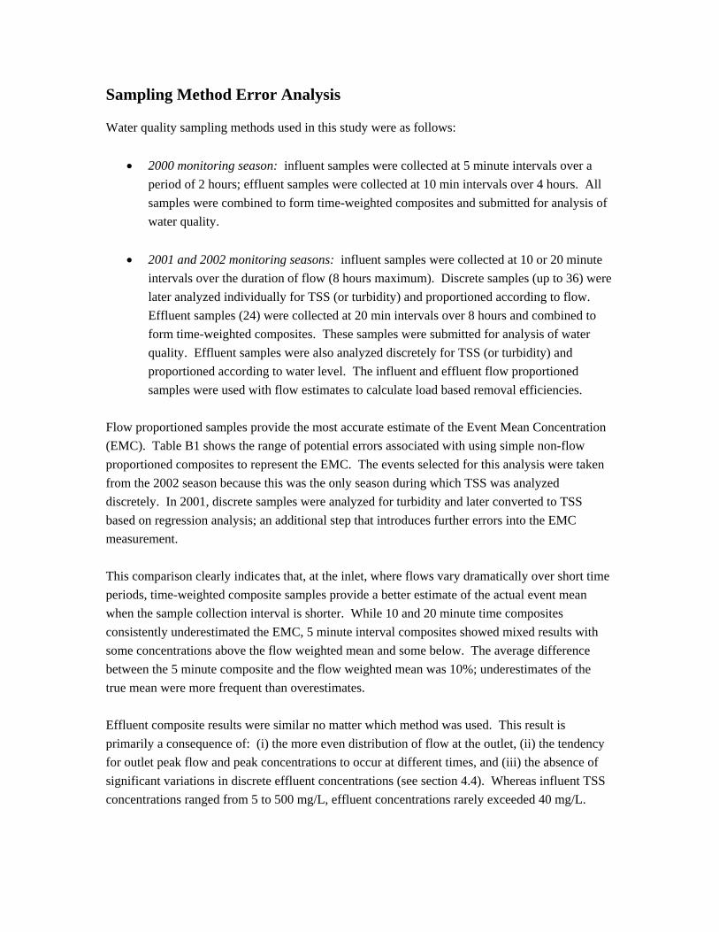
Sampling Method Error Analysis Water quality sampling methods used in this study were as follows:
2000 monitoring season: influent samples were collected at 5 minute intervals over a period of 2 hours; effluent samples were collected at 10 min intervals over 4 hours. All samples were combined to form time-weighted composites and submitted for analysis of water quality.
2001 and 2002 monitoring seasons: influent samples were collected at 10 or 20 minute
intervals over the duration of flow (8 hours maximum). Discrete samples (up to 36) were later analyzed individually for TSS (or turbidity) and proportioned according to flow. Effluent samples (24) were collected at 20 min intervals over 8 hours and combined to form time-weighted composites. These samples were submitted for analysis of water quality. Effluent samples were also analyzed discretely for TSS (or turbidity) and proportioned according to water level. The influent and effluent flow proportioned samples were used with flow estimates to calculate load based removal efficiencies.
Flow proportioned samples provide the most accurate estimate of the Event Mean Concentration (EMC). Table B1 shows the range of potential errors associated with using simple non-flow proportioned composites to represent the EMC. The events selected for this analysis were taken from the 2002 season because this was the only season during which TSS was analyzed discretely. In 2001, discrete samples were analyzed for turbidity and later converted to TSS based on regression analysis; an additional step that introduces further errors into the EMC measurement. This comparison clearly indicates that, at the inlet, where flows vary dramatically over short time periods, time-weighted composite samples provide a better estimate of the actual event mean when the sample collection interval is shorter. While 10 and 20 minute time composites consistently underestimated the EMC, 5 minute interval composites showed mixed results with some concentrations above the flow weighted mean and some below. The average difference between the 5 minute composite and the flow weighted mean was 10%; underestimates of the true mean were more frequent than overestimates. Effluent composite results were similar no matter which method was used. This result is primarily a consequence of: (i) the more even distribution of flow at the outlet, (ii) the tendency for outlet peak flow and peak concentrations to occur at different times, and (iii) the absence of significant variations in discrete effluent concentrations (see section 4.4). Whereas influent TSS concentrations ranged from 5 to 500 mg/L, effluent concentrations rarely exceeded 40 mg/L.

TableB1: Comparison of TSS concentrations determined by different methods.
Influent TSS Conc. (mg/L) Effluent TSS Conc. (mg/L) Simple Average~ Simple Average~
Date
Rain (mm)
5 min; 2 h
10 min. 4 h.
20 min. 8 h.
Flow Propor-tioned
10 min. 4 h.
20 min. 8 h.
Flow Propor-tioned+
May 31/02 6.8 142.0 80.7 46.2 131.7 13.3 13.5* 13.4
June 21/02 12.7 231.0 143.2 79.1 197.4 10.7 8.1 9.2
July 9/02 5.0 121.9 98.7 54.2 188.0 10.0 10.2 10.6
July 21/02 25.7 104.5 69.8 37.2 104.3 29.1 25.2 28.8
July 22/02 23.3 81.9 44.6 24.2 92.8 19.8 17.9 18.3
Aug 22/02 7.5 65.9 51.1* 51.5* 107.5 13.0 15.0 14.0
Sept 21/01++ 22.4 48.0 45.3 31.5 58.5 14.3 12.0 10.4
Mean 14.8 113.6 76.2 46.3 125.7 15.7 14.6 15.0 + Flow was not measured. Samples were proportioned according to outlet water level. * Samples collected over 5 hours (May 31) and 3.3 hours (Aug 22), but include the period of major flow. ~ Mean composite sample concentrations are based on 24 samples collected at the indicated time interval and duration, except where otherwise noted. ++ TSS concentrations are based on the conversion of discrete sample turbidity measurements to TSS (see section 3.5 for turbidity – TSS relationships) Overall, this analysis suggests that time weighted effluent concentration data provides a reasonably accurate depiction of the true mean effluent concentration and should, therefore, be relied upon as a central component of this performance assessment. The 2000 removal efficiency data is more prone to error. If the analysis provided here is representative of the 2000 season, and time weighted influent concentrations exceed flow weighted EMCs, then the reported results for the 2000 year of monitoring likely underestimates true removal. The removal efficiency data for the 2001 and 2002 season are based on flow proportioned samples and are, therefore, not subject to the errors associated with 2000 removal efficiency estimates.

APPENDIX C
Water Level Data

Figure C1 : Water level fluctuations in cells 1 to 3 during the 2000 monitoring season. Note that the water elevations are presented relative to an arbritrary dry-weather baseline.
0
100
200
300
400
500
600
700
800
900
09/06/0010:10
12/06/0021:30
16/06/0008:50
19/06/0020:10
23/06/0007:30
26/06/0018:50
30/06/0006:10
03/07/0017:30
07/07/0004:50
10/07/0016:10
14/07/0003:30
17/07/0014:50
21/07/0002:10
24/07/0013:30
28/07/0000:50
31/07/0012:10
03/08/0023:30
Wat
er le
vel (
mm
)
0
1
2
3
4
5
6
7
8
9
10
Rai
n (m
m)
0
100
200
300
400
500
600
07/08/0010:30
10/08/0021:50
14/08/0009:10
17/08/0020:30
21/08/0007:50
24/08/0019:10
28/08/0006:30
31/08/0017:50
04/09/0005:10
07/09/0016:30
11/09/0003:50
14/09/0015:10
18/09/0002:30
21/09/0013:50
25/09/0001:10
28/09/0012:30
01/10/0023:50
Wat
er le
vel (
mm
)
0
1
2
3
4
5
6
7
8
9
10
Rai
n (m
m)
0
100
200
300
400
500
600
05/10/0011:10
08/10/0022:30
12/10/0009:50
15/10/0021:10
19/10/0008:30
22/10/0019:50
26/10/0007:10
29/10/0018:30
02/11/0005:50
05/11/0017:10
09/11/0004:30
12/11/0015:50
Wat
er le
vel (
mm
)
0
1
2
3
4
5
6
7
8
9
10
Rai
n (m
m)

Figure C2 : Water level fluctuations in cells 1 to 3 during the 2001 monitoring season (May to August). Note that the water elevations are presented relative to an arbritrary dry-weather baseline.
0102030405060708090
100110120130140150160170180190200210
5/17/0114:05
5/22/0114:05
5/27/0114:05
6/1/0114:05
6/6/0114:05
6/11/0114:05
6/16/0114:05
6/21/0114:05
6/26/0114:05
7/1/0114:05
7/6/0114:05
Dep
th (m
m)
0
1
2
3
4
5
6
rainfall (mm
)
0102030405060708090
100110120130140150160170180190200210
7/8/0115:50
7/13/0115:50
7/18/0115:50
7/23/0115:50
7/28/0115:50
8/2/0115:50
8/7/0115:50
8/12/0115:50
8/17/0115:50
8/22/0115:50
8/27/0115:50
Dep
th (m
m)
0
1
2
3
4
5
6
rainfall (mm
)
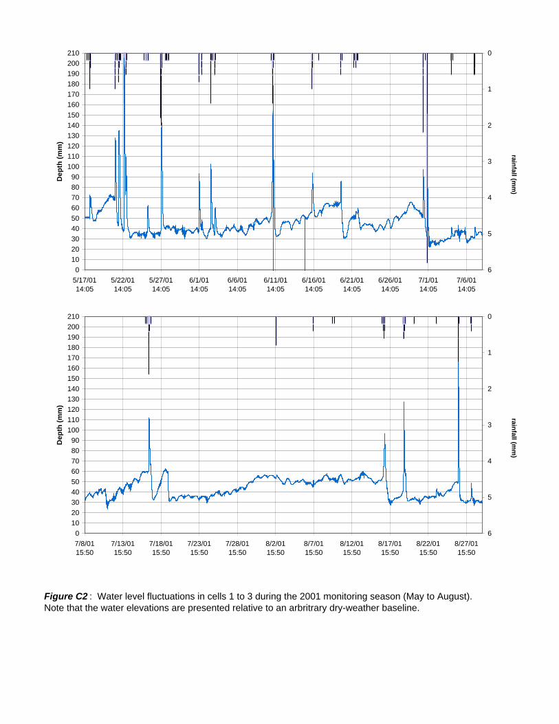

Figure C3 : Water level fluctuations in cells 1 to 3 during the 2002 monitoring season. Note that the water elevations and flows are presented relative to an arbritrary dry-weather baseline.
020406080
100120140160180200220240260280300320340360380400
5/22/0212:25
5/28/0212:25
6/3/0212:25
6/9/0212:25
6/15/0212:25
6/21/0212:25
6/27/0212:25
7/3/0212:25
7/9/0212:25
7/15/0212:25
7/21/0212:25
7/27/0212:25
Dep
th (m
m)
0
1
2
3
4
5
6
7
8
rainfall (mm
)
020406080
100120140160180200220240260280300320340360380400
7/27/0218:10
8/2/0218:10
8/8/0218:10
8/14/0218:10
8/20/0218:10
8/26/0218:10
9/1/0218:10
9/7/0218:10
9/13/0218:10
9/19/0218:10
9/25/0218:10
Dep
th (m
m)
0
1
2
3
4
5
6
7
8
rainfall (mm
)

APPENDIX D
Mass-based Analyisis of Two Rain Events
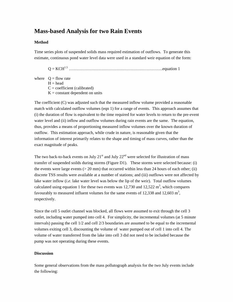
Mass-based Analysis for two Rain Events Method Time series plots of suspended solids mass required estimation of outflows. To generate this estimate, continuous pond water level data were used in a standard weir equation of the form:
Q = KCH1.5 ………………………………………………………….equation 1 where Q = flow rate H = head C = coefficient (calibrated) K = constant dependent on units The coefficient (C) was adjusted such that the measured inflow volume provided a reasonable match with calculated outflow volumes (eqn 1) for a range of events. This approach assumes that (i) the duration of flow is equivalent to the time required for water levels to return to the pre-event water level and (ii) inflow and outflow volumes during rain events are the same. The equation, thus, provides a means of proportioning measured inflow volumes over the known duration of outflow. This estimation approach, while crude in nature, is reasonable given that the information of interest primarily relates to the shape and timing of mass curves, rather than the exact magnitude of peaks. The two back-to-back events on July 21st and July 22nd were selected for illustration of mass transfer of suspended soilds during storms (Figure D1). These storms were selected because: (i) the events were large events (> 20 mm) that occurred within less than 24 hours of each other; (ii) discrete TSS results were available at a number of stations; and (iii) outflows were not affected by lake water inflow (i.e. lake water level was below the lip of the weir). Total outflow volumes calculated using equation 1 for these two events was 12,730 and 12,522 m3, which compares favourably to measured influent volumes for the same events of 12,338 and 12,603 m3, respectively. Since the cell 5 outlet channel was blocked, all flows were assumed to exit through the cell 3 outlet, including water pumped into cell 4. For simplicity, the incremental volumes (at 5 minute intervals) passing the cell 1/2 and cell 2/3 boundaries are assumed to be equal to the incremental volumes exiting cell 3, discounting the volume of water pumped out of cell 1 into cell 4. The volume of water transferred from the lake into cell 3 did not need to be included because the pump was not operating during these events. Discussion Some general observations from the mass pollutograph analysis for the two July events include the following:
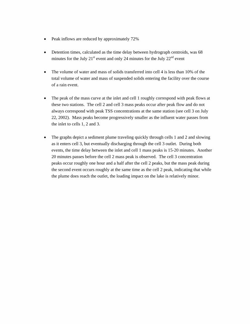
Peak inflows are reduced by approximately 72%
Detention times, calculated as the time delay between hydrograph centroids, was 68
minutes for the July 21st event and only 24 minutes for the July 22nd event
The volume of water and mass of solids transferred into cell 4 is less than 10% of the total volume of water and mass of suspended solids entering the facility over the course of a rain event.
The peak of the mass curve at the inlet and cell 1 roughly correspond with peak flows at
these two stations. The cell 2 and cell 3 mass peaks occur after peak flow and do not always correspond with peak TSS concentrations at the same station (see cell 3 on July 22, 2002). Mass peaks become progressively smaller as the influent water passes from the inlet to cells 1, 2 and 3.
The graphs depict a sediment plume traveling quickly through cells 1 and 2 and slowing
as it enters cell 3, but eventually discharging through the cell 3 outlet. During both events, the time delay between the inlet and cell 1 mass peaks is 15-20 minutes. Another 20 minutes passes before the cell 2 mass peak is observed. The cell 3 concentration peaks occur roughly one hour and a half after the cell 2 peaks, but the mass peak during the second event occurs roughly at the same time as the cell 2 peak, indicating that while the plume does reach the outlet, the loading impact on the lake is relatively minor.

July 21, 2002 -- 26 mm of rain over 2 hours and 25 minutes July 22, 2002 -- 23 mm of rain over 3 hours and 50 minutes
Figure D1 : Hydrographs, hyetographs and pollutographs for the back-to-back events on July 21 and July 22, 2002.
0
20
40
60
80
100
120
140
160
22:30 23:10 23:50 0:30 1:10 1:50 2:30 3:10 3:50 4:30 5:10 5:50
TSS
Con
cent
ratio
n (m
g/L)
InletCell 1Cell 2Cell 3Cell 4 in
0
1
2
3
4
5
6
22:30 23:10 23:50 0:30 1:10 1:50 2:30 3:10 3:50 4:30 5:10 5:50
Rai
n (m
m)
0
1000
2000
3000
4000
5000
6000
7000
8000
22:30 23:10 23:50 0:30 1:10 1:50 2:30 3:10 3:50 4:30 5:10 5:50
FLow
(L/s
)
inflow
cell 3 (outflow)
cell 4 (pumped inflow)
pump #2 is triggered at 12:05 AM and remains on for 60 hours
0
50
100
150
200
250
300
350
400
450
500
550
22:30 23:10 23:50 0:30 1:10 1:50 2:30 3:10 3:50 4:30 5:10 5:50
Mas
s (k
g)
InletCell 1Cell 2Cell 3Cell 4 in
0
1
2
3
4
5
6
14:40 15:20 16:00 16:40 17:20 18:00 18:40 19:20 20:00
Rai
n (m
m)
0
1000
2000
3000
4000
5000
6000
7000
8000
14:40 15:20 16:00 16:40 17:20 18:00 18:40 19:20 20:00
Flow
(L/s
)
inflow
cell 3 (outflow)cell 4 (pumped inflow)
0
20
40
60
80
100
120
140
160
14:40 15:20 16:00 16:40 17:20 18:00 18:40 19:20 20:00TS
S C
once
ntra
tion
(mg/
L)
Inlet
Cell 1
Cell 2
Cell 3
Cell 4 in
0
50
100
150
200
250
300
350
400
450
500
550
14:40 15:20 16:00 16:40 17:20 18:00 18:40 19:20 20:00
Mas
s (k
g)
Inlet
Cell 1
Cell 2
Cell 3
Cell 4 in

APPENDIX E
Individual Event Particle Size Distributions
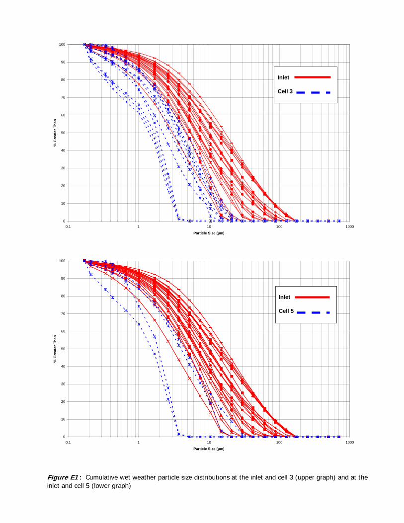
Figure E1 : Cumulative wet weather particle size distributions at the inlet and cell 3 (upper graph) and at the inlet and cell 5 (lower graph)
0
10
20
30
40
50
60
70
80
90
100
0.1 1 10 100 1000
Particle Size (µm)
% G
reat
er T
han
Inlet
Cell 3
0
10
20
30
40
50
60
70
80
90
100
0.1 1 10 100 1000
Particle Size (µm)
% G
reat
er T
han
Inlet
Cell 5

APPENDIX F
Water Quality Summary Statistics

Table F1: Wet weather water quality summary statistics -- Inlet (2000 monitoring season)
Category Parameter N RMDL %>DL MIN MAX MEDIAN GEOMETRIC MEAN FLOW WEIGHTED MEAN ARITHMETIC MEAN SD 95%CI -LL 95%CI -UL GUIDELINE % > GUIDELINEGeneral Suspended Solids (mg/L) 20 2.5 100 25 2460 76.75 89.62 139.00 218.95 534.36 -15.24 453.14Chemistry Dissolved Solids (mg/L) 20 10 100 96 514 214 240.59 249.49 262.60 116.44 211.57 313.63
Total Solids (mg/L) 20 10 100 210 2900 334 375.28 389.03 481.80 580.64 227.33 736.27Solvents Extractable (mg/L) 19 1 95 1 12 5 4.75 6.14 5.51 2.76 4.26 6.75Conductivity (uS/cm) 20 1 100 149 790 330 370.81 384.45 404.50 179.03 326.04 482.96pH 20 0.1 100 7.3 7.88 7.64 7.64 7.65 7.64 0.15 7.58 7.71Alkalinity (mg/L CaCO3) 20 2.5 100 43 124 70.25 75.25 74.80 78.10 22.56 68.21 87.99Turbidity (FTU) 20 0.01 100 14.7 2000 36.25 43.00 62.01 142.73 439.09 -49.71 335.16BOD (mg/L) 7 0.2 100 5 13.8 7.4 7.96 8.64 8.46 3.25 6.05 10.86Chloride (mg/L) 20 0.2 100 13.8 155 49.5 53.91 61.09 63.49 38.33 46.69 80.29 250.0 0Carbon (DOC) (mg/L) 20 0.1 100 3.2 16.3 7.1 7.14 7.31 7.89 3.82 6.21 9.57Carbon (DIC) (mg/L) 20 0.2 100 10.8 30.6 17.7 18.54 18.35 19.24 5.54 16.81 21.67Silicon (mg/L) 20 0.02 100 0.48 2.66 1.24 1.28 1.26 1.38 0.56 1.14 1.62
Metals Aluminum (ug/L) 20 11 100 121 1570 419 450.30 598.12 555.20 387.02 385.59 724.81Arsenic (ug/L) 20 1 0 0.5 1 0.5 0.55 0.51 0.58 0.18 0.49 0.66 0.1 100Barium (ug/L) 20 0.2 100 19.9 156 28.15 34.71 36.30 39.86 29.51 26.92 52.79Beryllium (ug/L) 20 0.2 5 0.01 0.246 0.0362 0.04 0.06 0.06 0.06 0.03 0.08 1100 0Cadmium (ug/L) 20 0.6 5 0.3 1.23 0.3 0.32 0.31 0.35 0.21 0.26 0.44 0.5 5Calcium (ug/L) 20 5 100 22500 204000 36350 41061.03 41721.31 47755.00 38784.99 30757.04 64752.96Chromium (ug/L) 20 1.4 95 0.7 7.83 2.87 2.92 3.22 3.27 1.58 2.58 3.96Cobalt (ug/L) 20 1.3 35 0.65 5.4 0.65 0.96 1.05 1.20 1.12 0.71 1.70 0.9 35Copper (ug/L) 20 1.6 100 2.5 50.5 19.35 19.50 21.82 22.16 10.38 17.61 26.71 5 95Iron (ug/L) 20 0.8 100 256 3690 668 747.16 991.58 952.15 812.86 595.91 1308.39 300 90Lead (ug/L) 20 10 45 5 62.1 5 9.43 14.47 13.26 13.73 7.24 19.28 5 45Magnesium (ug/L) 20 8 100 2390 11300 4720 5050.90 5321.37 5486.00 2414.14 4427.98 6544.02Manganese (ug/L) 20 0.2 100 34 849 93.25 108.23 156.97 159.50 185.37 78.26 240.74Mercury (ug/L) 20 0.02 30 0.01 0.09 0.01 0.02 0.03 0.02 0.03 0.01 0.04 0.2 0Molybdenum (ug/L) 20 1.6 15 0.8 51.6 0.8 1.09 2.03 3.48 11.33 -1.49 8.45 40 5Nickel (ug/L) 20 1.3 95 0.65 8.3 2.25 2.72 2.76 3.24 2.00 2.36 4.11 25 0Selenium (ug/L) 20 1 0 0.5 0.5 0.5 0.50 0.50 0.50 0.00Strontium (ug/L) 20 0.1 100 57 398 116.5 119.20 122.59 132.51 74.85 99.70 165.31Titanium (ug/L) 20 0.5 95 0.25 21.6 7.79 6.75 8.70 8.23 4.25 6.37 10.10Vanadium (ug/L) 20 1.5 90 0.75 8.9 2.565 2.62 3.05 3.02 1.78 2.25 3.80 6 5Zinc (ug/L) 20 0.6 100 5.72 223 62.8 66.47 79.64 79.76 46.43 59.41 100.11 20 95
Nutrients Nitrogen (NH3+NH4) (mg/L) 20 0.002 100 0.032 0.376 0.154 0.14 0.15 0.17 0.10 0.13 0.21Nitrogen (NO2) (mg/L) 20 0.001 100 0.015 0.5 0.1385 0.12 0.14 0.15 0.10 0.10 0.19Nitrogen (NO2+NO3) (mg/L) 20 0.005 100 0.085 2.24 1.09 0.88 1.17 1.14 0.63 0.87 1.42Phosphate (mg/L) 20 0.005 90 0.002 0.37 0.0605 0.05 0.06 0.08 0.08 0.04 0.11Total Phosphorus (mg/L) 20 0.002 100 0.004 2.11 0.307 0.28 0.39 0.45 0.46 0.25 0.65 0.03 95TKN Nitrogen (mg/L) 20 0.02 100 0.3 4.82 1.69 1.58 1.93 1.91 1.12 1.42 2.41
Bacteria Escherichia coli (c/100mL) 7 4 7600 46000 20000 19691.99 21184.89 22942.86 13392.39 13021.82 32863.90 100 100Fecal streptococcus (c/100mL) 7 4 4800 43000 30000 19559.12 12324.16 25800.00 15722.60 14152.75 37447.25Pseudomonas aeruginosa (c/100mL) 7 4 150 5300 2100 1367.11 1129.89 2141.43 1702.75 880.04 3402.82
Herbicides and 2,4,6 -trichlorophenol (ng/L) 2 20 100 28 32 30 29.93 30.29 30.00 2.83 26.08 33.92Pesticides Pentachlorophenol (ng/L) 0 10 0 0 0 0 0.00 0.00 0.00 0.00 500 0
Dicamba (ng/L) 11 50 100 52 240 84 92.25 126.30 107.27 65.01 68.85 145.69 200000 02,4 -D (ng/L) 17 100 100 160 3500 770 928.38 1420.68 1440.00 1236.41 852.26 2027.74 4000 0
PAH Fluoranthene (ug/L) 3 0.4 0 0.4 1 0.6 0.62 0.73 0.67 0.31 0.32 1.01Pyrene (ug/L) 3 0.4 33 0.2 0.8 0.4 0.40 0.53 0.47 0.31 0.12 0.81Chrysene (ug/L) 2 0.3 50 0.2 0.4 0.3 0.28 0.28 0.30 0.14 0.10 0.50
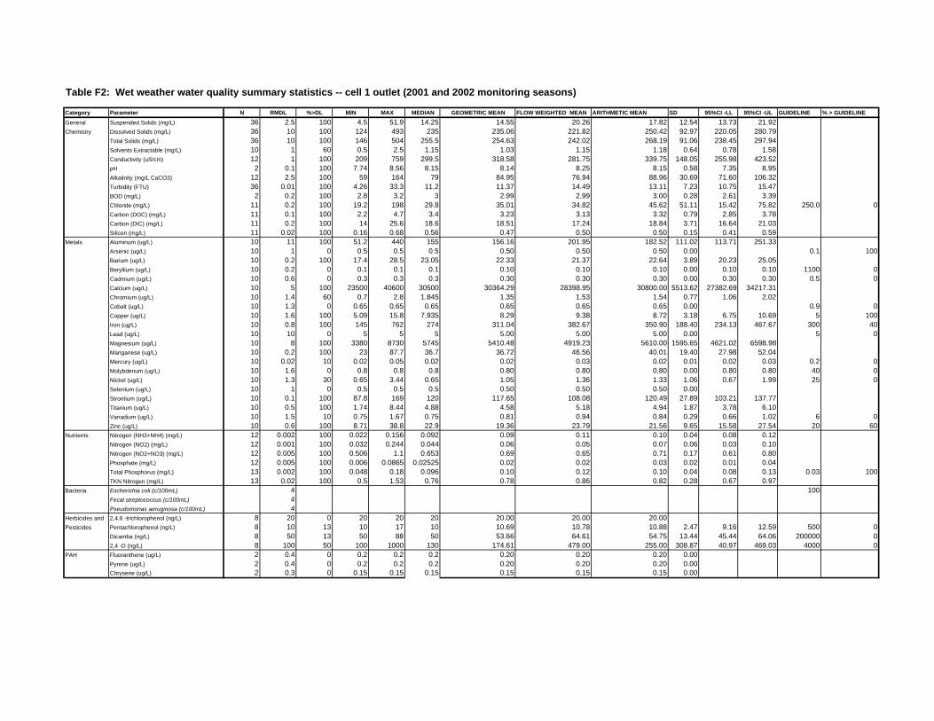
Table F2: Wet weather water quality summary statistics -- cell 1 outlet (2001 and 2002 monitoring seasons)
Category Parameter N RMDL %>DL MIN MAX MEDIAN GEOMETRIC MEAN FLOW WEIGHTED MEAN ARITHMETIC MEAN SD 95%CI -LL 95%CI -UL GUIDELINE % > GUIDELINEGeneral Suspended Solids (mg/L) 36 2.5 100 4.5 51.9 14.25 14.55 20.26 17.82 12.54 13.73 21.92Chemistry Dissolved Solids (mg/L) 36 10 100 124 493 235 235.06 221.82 250.42 92.97 220.05 280.79
Total Solids (mg/L) 36 10 100 146 504 255.5 254.63 242.02 268.19 91.06 238.45 297.94Solvents Extractable (mg/L) 10 1 60 0.5 2.5 1.15 1.03 1.15 1.18 0.64 0.78 1.58Conductivity (uS/cm) 12 1 100 209 759 299.5 318.58 281.75 339.75 148.05 255.98 423.52pH 2 0.1 100 7.74 8.56 8.15 8.14 8.25 8.15 0.58 7.35 8.95Alkalinity (mg/L CaCO3) 12 2.5 100 59 164 79 84.95 76.94 88.96 30.69 71.60 106.32Turbidity (FTU) 36 0.01 100 4.26 33.3 11.2 11.37 14.49 13.11 7.23 10.75 15.47BOD (mg/L) 2 0.2 100 2.8 3.2 3 2.99 2.99 3.00 0.28 2.61 3.39Chloride (mg/L) 11 0.2 100 19.2 198 29.8 35.01 34.82 45.62 51.11 15.42 75.82 250.0 0Carbon (DOC) (mg/L) 11 0.1 100 2.2 4.7 3.4 3.23 3.13 3.32 0.79 2.85 3.78Carbon (DIC) (mg/L) 11 0.2 100 14 25.6 18.6 18.51 17.24 18.84 3.71 16.64 21.03Silicon (mg/L) 11 0.02 100 0.16 0.68 0.56 0.47 0.50 0.50 0.15 0.41 0.59
Metals Aluminum (ug/L) 10 11 100 51.2 440 155 156.16 201.95 182.52 111.02 113.71 251.33Arsenic (ug/L) 10 1 0 0.5 0.5 0.5 0.50 0.50 0.50 0.00 0.1 100Barium (ug/L) 10 0.2 100 17.4 28.5 23.05 22.33 21.37 22.64 3.89 20.23 25.05Beryllium (ug/L) 10 0.2 0 0.1 0.1 0.1 0.10 0.10 0.10 0.00 0.10 0.10 1100 0Cadmium (ug/L) 10 0.6 0 0.3 0.3 0.3 0.30 0.30 0.30 0.00 0.30 0.30 0.5 0Calcium (ug/L) 10 5 100 23500 40600 30500 30364.29 28398.95 30800.00 5513.62 27382.69 34217.31Chromium (ug/L) 10 1.4 60 0.7 2.8 1.845 1.35 1.53 1.54 0.77 1.06 2.02Cobalt (ug/L) 10 1.3 0 0.65 0.65 0.65 0.65 0.65 0.65 0.00 0.9 0Copper (ug/L) 10 1.6 100 5.09 15.8 7.935 8.29 9.38 8.72 3.18 6.75 10.69 5 100Iron (ug/L) 10 0.8 100 145 762 274 311.04 382.67 350.90 188.40 234.13 467.67 300 40Lead (ug/L) 10 10 0 5 5 5 5.00 5.00 5.00 0.00 5 0Magnesium (ug/L) 10 8 100 3380 8730 5745 5410.48 4919.23 5610.00 1595.65 4621.02 6598.98Manganese (ug/L) 10 0.2 100 23 87.7 36.7 36.72 46.56 40.01 19.40 27.98 52.04Mercury (ug/L) 10 0.02 10 0.02 0.05 0.02 0.02 0.03 0.02 0.01 0.02 0.03 0.2 0Molybdenum (ug/L) 10 1.6 0 0.8 0.8 0.8 0.80 0.80 0.80 0.00 0.80 0.80 40 0Nickel (ug/L) 10 1.3 30 0.65 3.44 0.65 1.05 1.36 1.33 1.06 0.67 1.99 25 0Selenium (ug/L) 10 1 0 0.5 0.5 0.5 0.50 0.50 0.50 0.00Strontium (ug/L) 10 0.1 100 87.8 169 120 117.65 108.08 120.49 27.89 103.21 137.77Titanium (ug/L) 10 0.5 100 1.74 8.44 4.88 4.58 5.18 4.94 1.87 3.78 6.10Vanadium (ug/L) 10 1.5 10 0.75 1.67 0.75 0.81 0.94 0.84 0.29 0.66 1.02 6 0Zinc (ug/L) 10 0.6 100 8.71 38.8 22.9 19.36 23.79 21.56 9.65 15.58 27.54 20 60
Nutrients Nitrogen (NH3+NH4) (mg/L) 12 0.002 100 0.022 0.156 0.092 0.09 0.11 0.10 0.04 0.08 0.12Nitrogen (NO2) (mg/L) 12 0.001 100 0.032 0.244 0.044 0.06 0.05 0.07 0.06 0.03 0.10Nitrogen (NO2+NO3) (mg/L) 12 0.005 100 0.506 1.1 0.653 0.69 0.65 0.71 0.17 0.61 0.80Phosphate (mg/L) 12 0.005 100 0.006 0.0865 0.02525 0.02 0.02 0.03 0.02 0.01 0.04Total Phosphorus (mg/L) 13 0.002 100 0.048 0.18 0.096 0.10 0.12 0.10 0.04 0.08 0.13 0.03 100TKN Nitrogen (mg/L) 13 0.02 100 0.5 1.53 0.76 0.78 0.86 0.82 0.28 0.67 0.97
Bacteria Escherichia coli (c/100mL) 4 100Fecal streptococcus (c/100mL) 4Pseudomonas aeruginosa (c/100mL) 4
Herbicides and 2,4,6 -trichlorophenol (ng/L) 8 20 0 20 20 20 20.00 20.00 20.00Pesticides Pentachlorophenol (ng/L) 8 10 13 10 17 10 10.69 10.78 10.88 2.47 9.16 12.59 500 0
Dicamba (ng/L) 8 50 13 50 88 50 53.66 64.61 54.75 13.44 45.44 64.06 200000 02,4 -D (ng/L) 8 100 50 100 1000 130 174.61 479.00 255.00 308.87 40.97 469.03 4000 0
PAH Fluoranthene (ug/L) 2 0.4 0 0.2 0.2 0.2 0.20 0.20 0.20 0.00Pyrene (ug/L) 2 0.4 0 0.2 0.2 0.2 0.20 0.20 0.20 0.00Chrysene (ug/L) 2 0.3 0 0.15 0.15 0.15 0.15 0.15 0.15 0.00

Table F3: Wet weather water quality summary statistics -- cell 2 outlet (2001 and 2002 monitoring seasons)
Category Parameter N RMDL %>DL MIN MAX MEDIAN GEOMETRIC MEAN FLOW WEIGHTED MEAN ARITHMETIC MEAN SD 95%CI -LL 95%CI -UL GUIDELINE % > GUIDELINEGeneral Suspended Solids (mg/L) 32 2.5 100 4 38.1 10.25 10.44 12.86 12.33 7.93 9.58 15.08Chemistry Dissolved Solids (mg/L) 32 10 100 156 496 230 250.58 243.99 262.88 88.32 232.28 293.47
Total Solids (mg/L) 32 10 100 164 505 240 262.90 257.09 275.38 90.51 244.01 306.74Solvents Extractable (mg/L) 11 1 36 0.5 2 0.5 0.77 0.88 0.88 0.51 0.58 1.18Conductivity (uS/cm) 13 1 100 242 763 305 331.67 315.43 347.92 134.82 274.63 421.21pH 13 0.1 100 7.87 8.58 8.03 8.05 8.07 8.06 0.18 7.96 8.16Alkalinity (mg/L CaCO3) 13 2.5 100 68 194 88.5 92.38 96.43 96.27 33.44 78.09 114.45Turbidity (FTU) 32 0.01 100 3.56 20.8 8.2 8.73 10.48 9.80 4.87 8.11 11.48BOD (mg/L) 3 0.2 100 2 2.4 2 2.13 2.10 2.13 0.23 1.87 2.39Chloride (mg/L) 12 0.2 100 23.4 201 30.6 35.23 36.19 44.55 49.41 16.59 72.51 250.0 0.00Carbon (DOC) (mg/L) 12 0.1 100 2.1 3.9 2.7 2.73 2.75 2.78 0.51 2.49 3.06Carbon (DIC) (mg/L) 12 0.2 100 16 25.2 20.6 20.03 19.40 20.20 2.73 18.66 21.74Silicon (mg/L) 12 0.02 92 0.02 0.7 0.52 0.39 0.49 0.48 0.18 0.38 0.58
Metals Aluminum (ug/L) 11 11 100 46.4 269 92.2 95.38 115.70 107.20 61.39 70.92 143.48Arsenic (ug/L) 11 1 0 0.5 0.5 0.5 0.50 0.50 0.50 0.00 0.1 100.00Barium (ug/L) 11 0.2 100 18 24.9 22.1 21.93 21.61 22.03 2.13 20.77 23.29Beryllium (ug/L) 11 0.2 0 0.0161 0.1 0.1 0.08 0.08 0.09 0.03 0.08 0.11 1100 0.00Cadmium (ug/L) 11 0.6 0 0.0483 0.3 0.3 0.25 0.25 0.28 0.08 0.23 0.32 0.5 0.00Calcium (ug/L) 11 5 100 26800 39500 33900 33096.05 32195.18 33245.45 3275.47 31309.81 35181.10Chromium (ug/L) 11 1.4 18 0.7 1.59 0.7 0.80 0.87 0.85 0.33 0.65 1.04Cobalt (ug/L) 11 1.3 0 0.65 0.65 0.65 0.65 0.65 0.65 0.00 0.9 0.00Copper (ug/L) 11 1.6 100 3.15 9.78 5.56 5.52 5.95 5.78 1.86 4.69 6.88 5 72.73Iron (ug/L) 11 0.8 100 118 437 160 192.85 221.49 207.45 93.08 152.45 262.46 300 18.18Lead (ug/L) 11 10 0 3.76 5 5 4.87 4.78 4.89 0.37 4.67 5.11 5 0.00Magnesium (ug/L) 11 8 100 4440 8740 6050 6331.38 6127.23 6417.27 1104.17 5764.76 7069.78Manganese (ug/L) 11 0.2 100 18.8 43.7 24.4 25.11 28.48 25.88 7.18 21.64 30.13Mercury (ug/L) 11 0.02 0 0.02 0.02 0.02 0.02 0.02 0.02 0.00 0.02 0.02 0.2 0.00Molybdenum (ug/L) 11 1.6 36 0.585 4.93 0.8 1.22 1.52 1.60 1.42 0.76 2.44 40 0.00Nickel (ug/L) 11 1.3 100 0.65 4.66 0.65 1.03 1.23 1.34 1.26 0.60 2.09 25 0.00Selenium (ug/L) 11 1 0 0.5 0.5 0.5 0.50 0.50 0.50 0.00Strontium (ug/L) 11 0.1 100 106 167 138 134.51 130.29 135.45 16.72 125.57 145.34Titanium (ug/L) 11 0.5 100 1.62 7.7 3.33 3.22 3.62 3.51 1.64 2.55 4.48Vanadium (ug/L) 11 1.5 0 0.75 1.19 0.75 0.78 0.83 0.79 0.13 0.71 0.87 6 0.00Zinc (ug/L) 11 0.6 100 3.28 18.1 12.2 9.58 11.66 10.76 4.68 8.00 13.53 20 0.00
Nutrients Nitrogen (NH3+NH4) (mg/L) 13 0.002 100 0.074 0.426 0.124 0.13 0.14 0.15 0.09 0.10 0.20Nitrogen (NO2) (mg/L) 13 0.001 100 0.031 0.302 0.037 0.05 0.05 0.06 0.07 0.02 0.10Nitrogen (NO2+NO3) (mg/L) 13 0.005 100 0.322 0.722 0.603 0.55 0.56 0.57 0.14 0.49 0.64Phosphate (mg/L) 13 0.005 85 0.0025 0.022 0.018 0.01 0.01 0.01 0.01 0.01 0.02Total Phosphorus (mg/L) 14 0.002 100 0.034 0.18 0.058 0.06 0.08 0.07 0.04 0.05 0.09 0.03 100.00TKN Nitrogen (mg/L) 14 0.02 100 0.48 1.71 0.6 0.67 0.77 0.73 0.35 0.54 0.91
Bacteria Escherichia coli (c/100mL) 3 4 100 120 18000 840 1219.68 7254.22 6320.00 10121.58 -5133.44 17773.44 100 100.00Fecal streptococcus (c/100mL) 3 4 100 20 11000 2100 773.06 5060.95 4373.33 5832.34 -2226.45 10973.12Pseudomonas aeruginosa (c/100mL) 3 4 100 12 240 80 61.30 126.67 110.67 117.05 -21.79 243.12
Herbicides and 2,4,6 -trichlorophenol (ng/L) 9 20 0 20 20 20 20.00 21.43 20.00 0.00Pesticides Pentachlorophenol (ng/L) 9 10 0 10 10 10 10.00 10.72 10.00 0.00 500 0.00
Dicamba (ng/L) 9 50 11 50 180 50 57.65 97.35 64.44 43.33 36.13 92.76 200000 0.002,4 -D (ng/L) 9 100 44 100 500 100 144.33 266.07 171.11 131.29 85.34 256.88 4000 0.00
PAH Fluoranthene (ug/L) 2 0.4 0 0.2 0.2 0.2 0.20 0.20 0.20 0.00Pyrene (ug/L) 2 0.4 0 0.2 0.2 0.2 0.20 0.20 0.20 0.00Chrysene (ug/L) 2 0.3 0 0.15 0.2 0.175 0.17 0.19 0.18 0.04 0.13 0.22

Table F4: Wet weather water quality summary statistics -- cell 4 inlet (2000, 2001 and 2002 monitoring seasons)
Category Parameter N RMDL %>DL MIN MAX MEDIAN GEOMETRIC MEAN ARITHMETIC MEAN SD 95%CI -LL 95%CI -UL GUIDELINE % > GUIDELINEGeneral Suspended Solids (mg/L) 38 2.5 100 5.9 104 19.25 18.82 23.52 18.70 17.57 29.46Chemistry Dissolved Solids (mg/L) 38 10 100 140 459 232 243.38 253.24 73.74 229.79 276.68
Total Solids (mg/L) 38 10 100 172 480 256 267.46 276.87 74.77 253.09 300.64Solvents Extractable (mg/L) 36 1 64 0.25 4 1.35 1.15 1.41 0.85 1.13 1.69Conductivity (uS/cm) 38 1 100 214 706 356 370.68 386.05 114.41 349.68 422.43pH 38 0.1 100 7.59 8.45 7.975 7.97 7.97 0.16 7.92 8.02Alkalinity (mg/L CaCO3) 38 2.5 100 62 188 88.25 87.32 89.49 22.18 82.44 96.55Turbidity (FTU) 38 0.01 100 5.23 76.4 12.6 13.44 15.83 12.09 11.99 19.68BOD (mg/L) 11 0.2 100 1.4 7.4 3.6 3.40 3.84 1.92 2.70 4.97Chloride (mg/L) 38 0.2 100 20.4 188 42.8 48.14 56.93 37.73 44.94 68.93 250.0 0Carbon (DOC) (mg/L) 38 0.1 100 2.1 8.1 3.4 3.57 3.75 1.29 3.34 4.16Carbon (DIC) (mg/L) 38 0.2 100 13.6 28.8 20.9 20.30 20.66 3.82 19.44 21.87Silicon (mg/L) 38 0.02 100 0.16 1.38 0.59 0.55 0.61 0.27 0.53 0.70
Metals Aluminum (ug/L) 38 11 100 50.5 586 117.5 135.98 159.38 107.52 125.20 193.57Arsenic (ug/L) 39 1 0 0.5 1 0.5 0.52 0.53 0.11 0.49 0.56 0.1 100Barium (ug/L) 38 0.2 100 19.9 42.6 27.15 27.58 28.21 6.18 26.25 30.17Beryllium (ug/L) 38 0.2 0 0.00487 0.1 0.1 0.04 0.06 0.04 0.05 0.08 1100 0Cadmium (ug/L) 38 0.6 5 0.0261 0.918 0.3 0.28 0.32 0.16 0.27 0.37 0.5 5Calcium (ug/L) 38 5 100 22900 52200 34500 34744.45 35423.68 7094.40 33168.03 37679.34Chromium (ug/L) 38 1.4 34 0.102 3.05 0.7 0.92 1.10 0.70 0.88 1.32Cobalt (ug/L) 38 1.3 0 0.121 1.11 0.65 0.59 0.61 0.15 0.56 0.66 0.9 3Copper (ug/L) 38 1.6 100 2.11 40 6.96 6.67 7.74 5.97 5.84 9.64 5 74Iron (ug/L) 38 0.8 100 135 950 307.5 309.19 340.11 167.57 286.83 393.38 300 53Lead (ug/L) 38 10 3 0.258 11.6 5 4.49 4.85 1.48 4.38 5.32 5 5Magnesium (ug/L) 38 8 100 1070 9770 6415 6175.31 6522.37 1805.93 5948.18 7096.56Manganese (ug/L) 38 0.2 100 20.6 143 55.05 52.77 58.42 26.39 50.03 66.81Mercury (ug/L) 26 0.02 0 0.01 0.02 0.02 0.01 0.02 0.01 0.01 0.02 0.2 0Molybdenum (ug/L) 38 1.6 29 0.333 9.78 0.8 1.12 1.57 1.84 0.99 2.16 40 0Nickel (ug/L) 38 1.3 55 0.65 8.14 1.35 1.15 1.40 1.25 1.00 1.79 25 0Selenium (ug/L) 38 1 0 0.5 0.5 0.5 0.50 0.50 0.00Strontium (ug/L) 38 0.1 100 88.6 218 148.5 142.12 145.23 30.12 135.66 154.81Titanium (ug/L) 38 0.5 100 1.97 12 3.85 4.11 4.44 1.97 3.81 5.06Vanadium (ug/L) 38 1.5 13 0.45 2.4 0.75 0.88 0.94 0.43 0.81 1.08 6 0Zinc (ug/L) 38 0.6 100 3.36 34.4 17.8 15.57 17.75 8.33 15.11 20.40 20 42
Nutrients Nitrogen (NH3+NH4) (mg/L) 38 0.002 100 0.005 0.364 0.116 0.09 0.12 0.08 0.10 0.15Nitrogen (NO2) (mg/L) 38 0.001 100 0.009 0.321 0.0475 0.06 0.08 0.07 0.06 0.10Nitrogen (NO2+NO3) (mg/L) 38 0.005 100 0.182 1.46 0.645 0.60 0.68 0.32 0.58 0.78Phosphate (mg/L) 38 0.005 97 0.0025 0.0669 0.02 0.02 0.03 0.02 0.02 0.03Total Phosphorus (mg/L) 38 0.002 100 0.04 0.26 0.1096 0.10 0.12 0.06 0.10 0.14 0.03 100TKN Nitrogen (mg/L) 38 0.02 100 0.44 1.63 0.82 0.83 0.88 0.31 0.78 0.97
Bacteria Escherichia coli (c/100mL) 7 4 100 76 30000 2300 2342.57 8775.14 11575.07 200.37 17349.92 100 86Fecal streptococcus (c/100mL) 7 4 100 640 19000 2800 2654.38 5382.86 6802.91 343.29 10422.43Pseudomonas aeruginosa (c/100mL) 7 4 86 2 520 92 53.73 184.00 205.55 31.73 336.27
Herbicides an 2,4,6 -trichlorophenol (ng/L) 24 20 4 20 26 20 20.22 20.25 1.22 19.76 20.74Pesticides Pentachlorophenol (ng/L) 24 10 17 10 20 10 10.80 11.04 2.76 9.94 12.15 500 0
Dicamba (ng/L) 26 50 42 50 770 50 80.57 119.69 155.11 60.07 179.32 200000 02,4 -D (ng/L) 32 100 78 100 4100 295 356.32 688.13 990.66 344.88 1031.37 4000 3
PAH Fluoranthene (ug/L) 2 0.4 0 0.2 0.2 0.2 0.20 0.20 0.00Pyrene (ug/L) 2 0.4 0 0.2 0.2 0.2 0.20 0.20 0.00Chrysene (ug/L) 2 0.3 0 0.15 0.15 0.15 0.15 0.15 0.00

Table F5: Wet weather water quality summary statistics -- cell 4 outlet (2000, 2001 and 2002 monitoring seasons)
Category Parameter N RMDL %>DL MIN MAX MEDIAN GEOMETRIC MEAN ARITHMETIC MEAN SD 95%CI -LL 95%CI -UL GUIDELINE % > GUIDELINEGeneral Suspended Solids (mg/L) 38 2.5 100 3 35.5 9.75 9.57 10.78 6.18 8.82 12.75Chemistry Dissolved Solids (mg/L) 38 10 100 184 500 245 259.93 268.21 72.53 245.15 291.27
Total Solids (mg/L) 38 10 100 194 512 254 270.99 279.16 73.11 255.91 302.40Solvents Extractable (mg/L) 38 1 26 0.25 3 0.5 0.66 0.82 0.62 0.62 1.01Conductivity (uS/cm) 38 1 100 285 769 377.5 400.03 412.76 111.54 377.30 448.23pH 38 0.1 100 7.91 8.32 8.1 8.10 8.10 0.10 8.06 8.13Alkalinity (mg/L CaCO3) 38 2.5 100 79 108 96.75 95.04 95.39 8.17 92.79 97.99Turbidity (FTU) 38 0.01 100 2.93 25 8.24 8.62 9.46 4.30 8.09 10.83BOD (mg/L) 12 0.2 100 1 3.6 2.6 2.14 2.37 1.03 1.78 2.95Chloride (mg/L) 38 0.2 100 25.8 158 42.6 49.42 56.44 32.91 45.97 66.90 250.0 0Carbon (DOC) (mg/L) 38 0.1 100 0.67 8 3 2.96 3.15 1.24 2.76 3.54Carbon (DIC) (mg/L) 38 0.2 100 18.2 33.2 22.35 22.51 22.66 2.71 21.80 23.52Silicon (mg/L) 38 0.02 100 0.18 94 0.52 0.54 2.98 15.17 -1.85 7.80
Metals Aluminum (ug/L) 38 11 100 23.7 212 71.95 71.29 80.71 43.60 66.85 94.57Arsenic (ug/L) 38 1 0 0.5 1 0.5 0.51 0.51 0.08 0.49 0.54 0.1 100Barium (ug/L) 38 0.2 100 21.4 40 26.95 27.91 28.28 4.73 26.78 29.78Beryllium (ug/L) 38 0.2 0 0.00789 0.1 0.1 0.05 0.07 0.04 0.06 0.09 1100 0Cadmium (ug/L) 38 0.6 5 0.282 9.39 0.3 0.35 0.56 1.47 0.10 1.03 0.5 8Calcium (ug/L) 38 5 100 27100 42700 37300 36870.27 37084.21 3943.08 35830.52 38337.90Chromium (ug/L) 38 1.4 5 0.14 5.05 0.7 0.70 0.81 0.73 0.57 1.04Cobalt (ug/L) 38 1.3 3 0.0768 1.4 0.65 0.61 0.65 0.20 0.59 0.71 0.9 5Copper (ug/L) 38 1.6 84 0.8 81.3 3.735 3.60 6.31 12.81 2.24 10.39 5 34Iron (ug/L) 38 0.8 100 72.9 549 182.5 188.00 210.90 111.05 175.59 246.21 300 13Lead (ug/L) 38 10 3 0.39 38.2 5 4.66 5.62 5.55 3.85 7.38 5 5Magnesium (ug/L) 38 8 100 5580 9730 7750 7591.51 7673.16 1111.04 7319.91 8026.41Manganese (ug/L) 38 0.2 100 14.1 93.3 31.9 35.39 39.01 18.30 33.19 44.83Mercury (ug/L) 28 0.02 4 0.01 0.24 0.02 0.02 0.03 0.04 0.01 0.04 0.2 4Molybdenum (ug/L) 38 1.6 37 0.8 8.53 0.8 1.34 1.85 1.80 1.28 2.42 40 0Nickel (ug/L) 38 1.3 29 0.54 32 0.65 1.04 2.60 6.56 0.51 4.68 25 5Selenium (ug/L) 38 1 0 0.5 0.5 0.5 0.50 0.50 0.00Strontium (ug/L) 38 0.1 100 127 195 165.5 160.56 161.63 18.59 155.72 167.54Titanium (ug/L) 38 0.5 97 0.25 10 2.88 2.56 3.09 1.90 2.48 3.69Vanadium (ug/L) 38 1.5 3 0.218 2.48 0.75 0.76 0.80 0.30 0.70 0.89 6 0Zinc (ug/L) 38 0.6 100 0.656 244 6.04 5.69 12.00 38.72 -0.31 24.31 20 3
Nutrients Nitrogen (NH3+NH4) (mg/L) 38 0.002 95 0.002 0.281 0.136 0.10 0.13 0.07 0.11 0.16Nitrogen (NO2) (mg/L) 38 0.001 100 0.005 0.305 0.0315 0.04 0.05 0.06 0.03 0.07Nitrogen (NO2+NO3) (mg/L) 38 0.005 100 0.047 1.14 0.3955 0.34 0.43 0.27 0.35 0.51Phosphate (mg/L) 38 0.005 71 0.0025 0.0517 0.01025 0.01 0.01 0.01 0.01 0.02Total Phosphorus (mg/L) 38 0.002 100 0.032 0.146 0.056 0.07 0.07 0.03 0.06 0.08 0.03 100TKN Nitrogen (mg/L) 38 0.02 100 0.44 1.44 0.68 0.72 0.75 0.23 0.67 0.82
Bacteria Escherichia coli (c/100mL) 8 4 100 20 17000 330 274.79 2430.25 5899.74 -1657.98 6518.48 100 63Fecal streptococcus (c/100mL) 8 4 100 40 9600 300 273.40 1409.25 3313.72 -887.00 3705.50Pseudomonas aeruginosa (c/100mL) 8 4 50 2 1400 6 12.02 186.00 490.74 -154.06 526.06
Herbicides and 2,4,6 -trichlorophenol (ng/L) 24 20 4 20 24 20 20.15 20.17 0.82 19.84 20.49Pesticides Pentachlorophenol (ng/L) 23 10 0 10 10 10 10.00 10.00 0.00 500 0
Dicamba (ng/L) 23 50 22 50 2400 50 73.95 180.17 489.58 -19.91 380.25 200000 02,4 -D (ng/L) 28 100 64 100 24000 190 275.61 1282.86 4515.60 -389.71 2955.43 4000 4
PAH Fluoranthene (ug/L) 4 0.4 0 0.2 0.2 0.2 0.20 0.20 0.00Pyrene (ug/L) 4 0.4 0 0.2 0.2 0.2 0.20 0.20 0.00Chrysene (ug/L) 4 0.3 0 0.15 0.15 0.15 0.15 0.15 0.00

Table F6: Wet weather water quality summary statistics -- cell 3 oulet (2000, 2001 and 2002 monitoring seasons)
Category Parameter N RMDL %>DL MIN MAX MEDIAN GEOMETRIC MEAN FLOW WEIGHTED MEAN ARITHMETIC MEAN SD 95%CI -LL 95%CI -UL GUIDELINE % > GUIDELINEGeneral Suspended Solids (mg/L) 53 2.5 100 3.3 67 11 11.22 18.83 13.09 9.54 10.52 15.66Chemistry Dissolved Solids (mg/L) 53 10 100 160 486 232 252.93 256.91 263.04 80.12 241.47 284.61
Total Solids (mg/L) 53 10 100 170 495 244 266.17 275.47 276.02 80.55 254.33 297.70Solvents Extractable (mg/L) 50 1 36 0.25 4 0.95 0.83 1.17 1.04 0.77 0.83 1.25Conductivity (uS/cm) 52 1 100 247 748 362.5 391.00 396.98 406.58 123.45 373.02 440.13pH 52 0.1 100 7.41 8.56 8.065 8.05 8.01 8.05 0.18 8.01 8.10Alkalinity (mg/L CaCO3) 52 2.5 100 53.5 217 97.45 97.74 96.67 99.35 20.57 93.75 104.94Turbidity (FTU) 53 0.01 100 2.01 58.4 8.15 8.81 14.80 10.53 8.70 8.19 12.87BOD (mg/L) 12 0.2 100 1.2 4.4 2.7 2.37 2.86 2.57 1.02 1.99 3.14Chloride (mg/L) 52 0.2 100 23.8 212 38.5 46.85 53.80 56.48 41.94 45.08 67.88 250.0 0Carbon (DOC) (mg/L) 52 0.1 100 2 8.2 2.85 3.16 3.33 3.34 1.31 2.99 3.70Carbon (DIC) (mg/L) 52 0.2 100 18 31.2 22.8 23.02 22.91 23.18 2.81 22.41 23.94Silicon (mg/L) 52 0.02 98 0.02 1.08 0.46 0.42 0.53 0.52 0.29 0.44 0.60
Metals Aluminum (ug/L) 52 11 98 7.14 736 84.6 80.92 130.08 103.56 106.65 74.57 132.55Arsenic (ug/L) 52 1 0 0.5 0.5 0.5 0.50 0.50 0.50 0.00 5 0Barium (ug/L) 52 0.2 100 20.1 39.9 26.4 27.95 28.47 28.46 5.68 26.92 30.01Beryllium (ug/L) 52 0.2 0 0.000697 0.1 0.1 0.03 0.05 0.06 0.04 0.05 0.07 1100 0Cadmium (ug/L) 52 0.6 6 0.043 0.875 0.3 0.31 0.37 0.33 0.13 0.30 0.37 0.5 10Calcium (ug/L) 52 5 100 29700 50200 37000 37811.63 37752.75 38105.77 4891.67 36776.22 39435.31Chromium (ug/L) 52 1.4 6 0.0733 3.01 0.7 0.64 0.79 0.74 0.44 0.62 0.86Cobalt (ug/L) 52 1.3 2 0.331 5.36 0.65 0.65 1.02 0.72 0.66 0.54 0.90 0.9 2Copper (ug/L) 52 1.6 94 0.8 52.3 3.95 4.13 5.21 5.95 8.03 3.76 8.13 5 37Iron (ug/L) 52 0.8 100 2.76 1450 192 188.83 270.10 234.40 197.08 180.83 287.97 300 17Lead (ug/L) 52 10 2 0.14 15.7 5 4.66 5.19 5.03 1.72 4.56 5.50 5 4Magnesium (ug/L) 52 8 100 5160 11900 7880 7731.97 7553.51 7828.65 1245.19 7490.21 8167.09Manganese (ug/L) 52 0.2 98 0.134 206 33.25 33.85 56.05 45.62 35.26 36.04 55.21Mercury (ug/L) 37 0.02 3 0.01 0.2 0.02 0.02 0.02 0.02 0.03 0.01 0.03 0.2 0Molybdenum (ug/L) 52 1.6 27 0.223 10.1 0.8 1.11 1.14 1.53 1.81 1.04 2.02 40 0Nickel (ug/L) 52 1.3 35 0.0531 3.84 0.65 0.89 1.09 1.11 0.81 0.89 1.33 25 0Selenium (ug/L) 52 1 0 0.5 0.5 0.5 0.50 0.50 0.50 0.00Strontium (ug/L) 52 0.1 100 121 237 165 161.74 158.68 162.98 20.59 157.38 168.58Titanium (ug/L) 52 0.5 98 0.25 13.4 3.095 2.84 3.85 3.43 2.23 2.82 4.03Vanadium (ug/L) 52 1.5 2 0.164 3.08 0.75 0.69 0.79 0.75 0.37 0.65 0.85 6 0Zinc (ug/L) 52 0.6 100 2.23 106 5.855 6.74 11.68 9.10 14.26 5.23 12.98 20 2
Nutrients Nitrogen (NH3+NH4) (mg/L) 52 0.002 98 0.001 0.506 0.123 0.09 0.15 0.13 0.09 0.11 0.15Nitrogen (NO2) (mg/L) 52 0.001 100 0.003 0.528 0.035 0.04 0.07 0.05 0.08 0.03 0.07Nitrogen (NO2+NO3) (mg/L) 52 0.005 100 0.121 1.16 0.448 0.41 0.47 0.47 0.24 0.41 0.54Phosphate (mg/L) 52 0.005 69 0.00025 0.039 0.0085 0.01 0.01 0.01 0.01 0.01 0.01Total Phosphorus (mg/L) 52 0.002 100 0.028 0.156 0.052 0.06 0.08 0.07 0.03 0.06 0.07 0.03 98TKN Nitrogen (mg/L) 52 0.02 100 0.4 1.76 0.63 0.68 0.77 0.72 0.27 0.64 0.79
Bacteria Escherichia coli (c/100mL) 11 4 100 10 9000 240 278.96 4199.13 1730.73 2795.66 78.63 3382.83 100 64Fecal streptococcus (c/100mL) 11 4 91 4 5700 500 234.57 3147.57 1298.00 1851.51 203.85 2392.15Pseudomonas aeruginosa (c/100mL) 11 4 64 2 290 28 20.50 106.13 70.55 94.14 14.92 126.18
Herbicides an 2,4,6 -trichlorophenol (ng/L) 30 20 7 20 48 20 20.82 20.56 21.20 5.27 19.31 23.09Pesticides Pentachlorophenol (ng/L) 30 10 7 10 19 10 10.36 11.20 10.47 1.85 9.80 11.13 500 0
Dicamba (ng/L) 30 50 13 50 340 50 58.40 67.60 68.07 59.22 46.88 89.26 200000 02,4 -D (ng/L) 38 100 58 100 2300 140 207.57 199.67 367.11 513.93 203.70 530.51 4000 0
PAH Fluoranthene (ug/L) 4 0.4 0 0.2 0.2 0.2 0.20 0.20 0.20 0.00Pyrene (ug/L) 4 0.4 0 0.2 0.2 0.2 0.20 0.20 0.20 0.00Chrysene (ug/L) 4 0.3 0 0.15 0.15 0.15 0.15 0.15 0.15 0.00
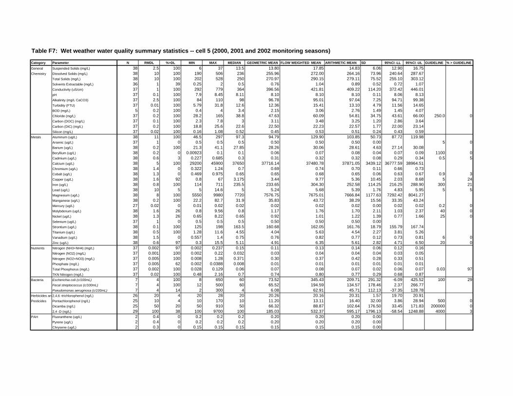
Table F7: Wet weather water quality summary statistics -- cell 5 (2000, 2001 and 2002 monitoring seasons)
Category Parameter N RMDL %>DL MIN MAX MEDIAN GEOMETRIC MEAN FLOW WEIGHTED MEAN ARITHMETIC MEAN SD 95%CI -LL 95%CI -UL GUIDELINE % > GUIDELINEGeneral Suspended Solids (mg/L) 38 2.5 100 6 37 13.5 13.80 17.85 14.83 6.06 12.90 16.75Chemistry Dissolved Solids (mg/L) 38 10 100 190 506 236 255.96 272.00 264.16 73.96 240.64 287.67
Total Solids (mg/L) 38 10 100 202 528 250 270.97 290.15 279.11 75.52 255.10 303.12Solvents Extractable (mg/L) 36 1 39 0.25 2 0.5 0.76 1.04 0.89 0.52 0.72 1.07Conductivity (uS/cm) 37 1 100 292 779 364 396.56 421.81 409.22 114.20 372.42 446.01pH 37 0.1 100 7.9 8.45 8.11 8.10 8.10 8.10 0.11 8.06 8.13Alkalinity (mg/L CaCO3) 37 2.5 100 84 110 98 96.78 95.01 97.04 7.25 94.71 99.38Turbidity (FTU) 37 0.01 100 5.79 31.8 12.6 12.36 15.41 13.10 4.79 11.56 14.65BOD (mg/L) 5 0.2 100 0.4 4 3.4 2.15 3.06 2.76 1.49 1.45 4.07Chloride (mg/L) 37 0.2 100 28.2 165 38.8 47.63 60.09 54.81 34.75 43.61 66.00 250.0 0Carbon (DOC) (mg/L) 37 0.1 100 2.3 7.8 3 3.11 3.48 3.25 1.20 2.86 3.64Carbon (DIC) (mg/L) 37 0.2 100 18.8 25.6 22.6 22.50 22.23 22.57 1.77 22.00 23.14Silicon (mg/L) 37 0.02 100 0.16 1.08 0.52 0.45 0.53 0.51 0.24 0.43 0.59
Metals Aluminum (ug/L) 38 11 100 46.5 297 97.3 94.79 129.90 103.85 50.73 87.72 119.98Arsenic (ug/L) 37 1 0 0.5 0.5 0.5 0.50 0.50 0.50 0.00 5 0Barium (ug/L) 38 0.2 100 21.3 41.1 27.85 28.26 30.06 28.61 4.63 27.14 30.08Beryllium (ug/L) 38 0.2 0 0.00923 0.1 0.1 0.06 0.07 0.08 0.04 0.07 0.09 1100 0Cadmium (ug/L) 38 0.6 3 0.227 0.685 0.3 0.31 0.32 0.32 0.08 0.29 0.34 0.5 5Calcium (ug/L) 38 5 100 29200 45900 37650 37716.14 37480.78 37871.05 3439.12 36777.59 38964.51Chromium (ug/L) 38 1.4 0 0.322 1.24 0.7 0.69 0.74 0.70 0.11 0.66 0.73Cobalt (ug/L) 38 1.3 0 0.469 0.975 0.65 0.65 0.68 0.65 0.06 0.63 0.67 0.9 3Copper (ug/L) 38 1.6 92 0.8 67 3.175 3.44 9.77 5.36 10.45 2.03 8.68 5 24Iron (ug/L) 38 0.8 100 114 711 235.5 233.65 304.30 252.58 114.25 216.25 288.90 300 21Lead (ug/L) 38 10 5 5 14.6 5 5.24 5.68 5.39 1.76 4.83 5.95 5 5Magnesium (ug/L) 38 8 100 5550 9980 7720 7576.75 7675.01 7666.84 1177.63 7292.42 8041.27Manganese (ug/L) 38 0.2 100 22.2 82.7 31.9 35.83 43.72 38.29 15.56 33.35 43.24Mercury (ug/L) 27 0.02 0 0.01 0.02 0.02 0.02 0.02 0.02 0.00 0.02 0.02 0.2 0Molybdenum (ug/L) 38 1.6 26 0.8 9.56 0.8 1.17 1.76 1.70 2.11 1.03 2.37 40 0Nickel (ug/L) 38 1.3 26 0.65 8.22 0.65 0.92 1.01 1.22 1.39 0.77 1.66 25 0Selenium (ug/L) 37 1 0 0.5 0.5 0.5 0.50 0.50 0.50 0.00Strontium (ug/L) 38 0.1 100 125 198 163.5 160.68 162.05 161.76 18.79 155.79 167.74Titanium (ug/L) 38 0.5 100 1.28 11.6 4.55 4.04 5.63 4.54 2.27 3.81 5.26Vanadium (ug/L) 38 1.5 0 0.557 1.4 0.75 0.76 0.82 0.77 0.12 0.73 0.81 6 0Zinc (ug/L) 38 0.6 97 0.3 15.5 5.11 4.91 6.35 5.61 2.82 4.71 6.50 20 0
Nutrients Nitrogen (NH3+NH4) (mg/L) 37 0.002 97 0.002 0.237 0.15 0.11 0.13 0.14 0.06 0.12 0.16Nitrogen (NO2) (mg/L) 37 0.001 100 0.002 0.22 0.032 0.03 0.04 0.04 0.04 0.03 0.05Nitrogen (NO2+NO3) (mg/L) 37 0.005 100 0.008 1.28 0.371 0.30 0.37 0.42 0.28 0.33 0.51Phosphate (mg/L) 37 0.005 62 0.002 0.0388 0.008 0.01 0.01 0.01 0.01 0.01 0.01Total Phosphorus (mg/L) 37 0.002 100 0.028 0.129 0.06 0.07 0.08 0.07 0.02 0.06 0.07 0.03 97TKN Nitrogen (mg/L) 37 0.02 100 0.48 2.16 0.7 0.74 0.80 0.77 0.29 0.68 0.87
Bacteria Escherichia coli (c/100mL) 7 4 100 8 650 60 73.52 345.43 209.71 291.32 -6.09 425.52 100 29Fecal streptococcus (c/100mL) 7 4 100 12 500 60 65.52 194.59 134.57 178.46 2.37 266.77Pseudomonas aeruginosa (c/100mL) 7 4 14 2 300 4 6.08 62.91 45.71 112.13 -37.35 128.78
Herbicides an 2,4,6 -trichlorophenol (ng/L) 26 20 4 20 28 20 20.26 20.16 20.31 1.57 19.70 20.91Pesticides Pentachlorophenol (ng/L) 25 10 4 10 170 10 11.20 13.11 16.40 32.00 3.86 28.94 500 0
Dicamba (ng/L) 25 50 20 50 910 50 66.32 88.87 102.64 176.50 33.45 171.83 200000 02,4 -D (ng/L) 29 100 38 100 9700 100 185.03 532.37 595.17 1796.13 -58.54 1248.88 4000 3
PAH Fluoranthene (ug/L) 2 0.4 0 0.2 0.2 0.2 0.20 0.20 0.20 0.00Pyrene (ug/L) 2 0.4 0 0.2 0.2 0.2 0.20 0.20 0.20 0.00Chrysene (ug/L) 2 0.3 0 0.15 0.15 0.15 0.15 0.15 0.15 0.00
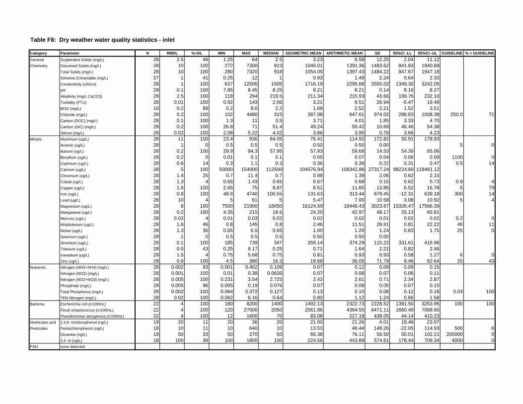
Table F8: Dry weather water quality statistics - inlet
Category Parameter N RMDL %>DL MIN MAX MEDIAN GEOMETRIC MEAN ARITHMETIC MEAN SD 95%CI -LL 95%CI -UL GUIDELINE % > GUIDELINEGeneral Suspended Solids (mg/L) 28 2.5 46 1.25 64 2.5 3.23 6.58 12.25 2.04 11.12Chemistry Dissolved Solids (mg/L) 28 10 100 272 7300 913 1046.01 1391.36 1483.62 841.83 1940.89
Total Solids (mg/L) 28 10 100 280 7320 918 1054.05 1397.43 1484.22 847.67 1947.18Solvents Extractable (mg/L) 27 1 41 0.25 12 1 0.93 1.49 2.24 0.64 2.33Conductivity (uS/cm) 28 1 100 637 12500 1505 1716.19 2295.68 2555.02 1349.30 3242.05pH 28 0.1 100 7.85 8.45 8.25 8.21 8.21 0.14 8.16 8.27Alkalinity (mg/L CaCO3) 28 2.5 100 118 294 219.5 211.34 215.93 43.66 199.76 232.10Turbidity (FTU) 28 0.01 100 0.92 143 2.06 3.21 9.51 26.94 -0.47 19.49BOD (mg/L) 19 0.2 89 0.2 8.6 2.2 1.69 2.52 2.21 1.52 3.51Chloride (mg/L) 28 0.2 100 102 4480 315 387.98 647.61 974.02 286.83 1008.38 250.0 71Carbon (DOC) (mg/L) 28 0.1 100 1.3 11 3.5 3.71 4.01 1.85 3.33 4.70Carbon (DIC) (mg/L) 28 0.2 100 26.8 71 51.4 49.24 50.42 10.69 46.46 54.38Silicon (mg/L) 28 0.02 100 2.08 5.22 4.02 3.86 3.95 0.78 3.66 4.23
Metals Aluminum (ug/L) 28 11 100 23.4 936 64.05 76.41 114.92 172.82 50.91 178.93Arsenic (ug/L) 28 1 0 0.5 0.5 0.5 0.50 0.50 0.00 5 0Barium (ug/L) 28 0.2 100 29.9 94.3 57.95 57.93 59.68 14.53 54.30 65.06Beryllium (ug/L) 28 0.2 0 0.01 0.1 0.1 0.05 0.07 0.04 0.06 0.09 1100 0Cadmium (ug/L) 28 0.6 14 0.3 1.1 0.3 0.36 0.39 0.22 0.31 0.47 0.5 14Calcium (ug/L) 28 5 100 50000 154000 112500 104576.94 108342.86 27317.24 98224.60 118461.12Chromium (ug/L) 28 1.4 25 0.7 11.4 0.7 0.98 1.39 2.06 0.62 2.15Cobalt (ug/L) 28 1.3 4 0.65 1.43 0.65 0.67 0.68 0.15 0.62 0.73 0.9 4Copper (ug/L) 28 1.6 100 2.65 75 8.87 8.51 11.65 13.85 6.52 16.78 5 79Iron (ug/L) 28 0.8 100 48.8 4740 100.55 131.63 313.44 879.45 -12.31 639.18 300 14Lead (ug/L) 28 10 4 5 61 5 5.47 7.00 10.58 3.08 10.92 5 4Magnesium (ug/L) 28 8 100 7500 21900 16650 16124.69 16446.43 3023.67 15326.47 17566.39Manganese (ug/L) 28 0.2 100 4.35 215 18.6 24.20 42.97 48.17 25.13 60.81Mercury (ug/L) 28 0.02 4 0.01 0.03 0.02 0.02 0.02 0.01 0.02 0.02 0.2 0Molybdenum (ug/L) 28 1.6 46 0.8 145 0.8 2.46 11.51 28.91 0.81 22.22 40 11Nickel (ug/L) 28 1.3 36 0.65 6.5 0.65 1.00 1.29 1.24 0.83 1.75 25 0Selenium (ug/L) 28 1 0 0.5 0.5 0.5 0.50 0.50 0.00Strontium (ug/L) 28 0.1 100 185 739 347 359.14 374.29 115.22 331.61 416.96Titanium (ug/L) 28 0.5 43 0.25 8.17 0.25 0.71 1.64 2.21 0.82 2.46Vanadium (ug/L) 28 1.5 4 0.75 5.68 0.75 0.81 0.93 0.93 0.58 1.27 6 0Zinc (ug/L) 28 0.6 100 4.5 390 16.3 19.68 36.05 71.79 9.46 62.64 20 43
Nutrients Nitrogen (NH3+NH4) (mg/L) 28 0.002 93 0.001 0.402 0.109 0.07 0.12 0.09 0.09 0.15Nitrogen (NO2) (mg/L) 28 0.001 100 0.01 0.38 0.0635 0.07 0.08 0.07 0.06 0.11Nitrogen (NO2+NO3) (mg/L) 28 0.005 100 0.231 3.54 2.725 2.42 2.61 0.71 2.34 2.87Phosphate (mg/L) 28 0.005 96 0.005 0.19 0.076 0.07 0.08 0.05 0.07 0.10Total Phosphorus (mg/L) 28 0.002 100 0.064 0.372 0.127 0.13 0.15 0.08 0.12 0.18 0.03 100TKN Nitrogen (mg/L) 28 0.02 100 0.062 6.16 0.64 0.80 1.12 1.24 0.66 1.58
Bacteria Escherichia coli (c/100mL) 22 4 100 180 8200 1400 1492.13 2322.73 2228.52 1391.50 3253.95 100 100Fecal streptococcus (c/100mL) 22 4 100 120 27000 2050 2061.86 4364.55 6471.11 1660.49 7068.60Pseudomonas aeruginosa (c/100mL) 22 4 100 12 1600 70 83.08 227.18 438.05 44.14 410.23
Herbicides and 2,4,6 -trichlorophenol (ng/L) 19 20 11 20 36 20 21.00 21.26 4.01 19.46 23.07Pesticides Pentachlorophenol (ng/L) 18 10 11 10 640 10 13.53 46.44 148.26 -22.05 114.93 500 6
Dicamba (ng/L) 18 50 33 50 270 50 65.38 76.11 56.50 50.01 102.21 200000 02,4 -D (ng/L) 18 100 39 100 1800 100 224.56 443.89 574.61 178.44 709.34 4000 0
PAH none detected

Table F9: Dry weather water quality statistics - Cell 4 inlet
Category Parameter N RMDL %>DL MIN MAX MEDIAN GEOMETRIC MEAN ARITHMETIC MEAN SD 95%CI -LL 95%CI -UL GUIDELINE % > GUIDELINEGeneral Suspended Solids (mg/L) 10 2.5 100 6 19 11.25 11.66 12.30 4.16 9.72 14.88Chemistry Dissolved Solids (mg/L) 10 10 100 184 274 226 223.46 224.80 25.89 208.75 240.85
Total Solids (mg/L) 10 10 100 196 284 239 235.76 237.00 25.51 221.19 252.81Solvents Extractable (mg/L) 10 1 30 0.25 1.6 0.5 0.68 0.81 0.49 0.50 1.11Conductivity (uS/cm) 10 1 100 284 421 348.5 343.91 345.90 39.12 321.65 370.15pH 10 0.1 100 7.85 8.39 8.105 8.11 8.11 0.15 8.02 8.21Alkalinity (mg/L CaCO3) 10 2.5 100 86 108 98.25 95.87 96.15 7.71 91.37 100.93Turbidity (FTU) 10 0.01 100 4.77 14.8 9.955 9.20 9.73 3.18 7.76 11.70BOD (mg/L) 7 0.2 100 2.2 4.8 2.8 3.07 3.17 0.91 2.50 3.84Chloride (mg/L) 10 0.2 100 28.8 53.6 36.6 36.76 37.36 7.37 32.79 41.93 250.0 0Carbon (DOC) (mg/L) 10 0.1 100 2.2 3.5 3 2.91 2.95 0.47 2.66 3.24Carbon (DIC) (mg/L) 10 0.2 100 19.6 25.2 22.3 22.19 22.26 1.89 21.09 23.43Silicon (mg/L) 10 0.02 100 0.24 0.8 0.38 0.40 0.44 0.19 0.32 0.55
Metals Aluminum (ug/L) 10 11 100 39.1 156 77.5 74.99 81.08 34.65 59.61 102.55Arsenic (ug/L) 10 1 0 0.5 0.5 0.5 0.50 0.50 0.00 0.1 100Barium (ug/L) 10 0.2 100 23 30 26.4 26.26 26.37 2.49 24.83 27.91Beryllium (ug/L) 10 0.2 0 0.01 0.1 0.1 0.07 0.08 0.04 0.06 0.11 1100 0Cadmium (ug/L) 10 0.6 0 0.3 0.3 0.3 0.30 0.30 0.00 0.30 0.30 0.5 0Calcium (ug/L) 10 5 100 30300 41400 36900 36486.68 36640.00 3471.54 34488.36 38791.64Chromium (ug/L) 10 1.4 0 0.7 0.7 0.7 0.70 0.70 0.00Cobalt (ug/L) 10 1.3 0 0.65 0.65 0.65 0.65 0.65 0.00 0.9 0Copper (ug/L) 10 1.6 60 0.8 5.71 1.74 1.68 2.14 1.61 1.14 3.13 5 10Iron (ug/L) 10 0.8 100 115 381 182.5 207.24 221.30 85.43 168.35 274.25 300 10Lead (ug/L) 10 10 0 5 5 5 5.00 5.00 0.00 5 0Magnesium (ug/L) 10 8 100 5240 9190 7790 7256.09 7399.00 1477.07 6483.52 8314.48Manganese (ug/L) 10 0.2 100 27.2 71.9 37.5 37.99 39.77 13.79 31.22 48.32Mercury (ug/L) 10 0.02 0 0.01 0.02 0.02 0.02 0.02 0.00 0.02 0.02 0.2 0Molybdenum (ug/L) 10 1.6 30 0.8 4.98 0.8 1.27 1.64 1.43 0.75 2.52 40 0Nickel (ug/L) 10 1.3 30 0.65 3.71 0.65 0.91 1.11 0.97 0.51 1.71 25 0Selenium (ug/L) 10 1 0 0.5 0.5 0.5 0.50 0.50 0.00Strontium (ug/L) 10 0.1 100 124 182 162 153.68 155.10 21.66 141.68 168.52Titanium (ug/L) 10 0.5 100 1.2 6.68 2.515 2.71 3.09 1.68 2.05 4.13Vanadium (ug/L) 10 1.5 0 0.75 0.75 0.75 0.75 0.75 0.00 6 0Zinc (ug/L) 10 0.6 100 2.69 11.5 5.65 5.38 6.07 3.07 4.17 7.98 20 0
Nutrients Nitrogen (NH3+NH4) (mg/L) 10 0.002 100 0.036 0.22 0.136 0.10 0.12 0.06 0.08 0.15Nitrogen (NO2) (mg/L) 10 0.001 100 0.018 0.061 0.035 0.03 0.04 0.01 0.03 0.04Nitrogen (NO2+NO3) (mg/L) 10 0.005 100 0.181 0.621 0.3555 0.34 0.36 0.15 0.27 0.45Phosphate (mg/L) 10 0.005 50 0.0025 0.015 0.006 0.01 0.01 0.00 0.00 0.01Total Phosphorus (mg/L) 10 0.002 100 0.034 0.112 0.053 0.06 0.06 0.02 0.05 0.07 0.03 100TKN Nitrogen (mg/L) 10 0.02 100 0.48 0.96 0.65 0.66 0.68 0.13 0.59 0.76
Bacteria Escherichia coli (c/100mL) 8 4 100 20 1800 140 153.98 393.75 606.16 -26.29 813.79 100 63Fecal streptococcus (c/100mL) 8 4 100 10 860 50 65.79 221.25 342.86 -16.34 458.84Pseudomonas aeruginosa (c/100mL) 8 4 38 4 30 4 6.29 8.50 8.99 2.27 14.73
Herbicides and 2,4,6 -trichlorophenol (ng/L) 8 20 0 20 20 20 20.00 20.00 0.00Pesticides Pentachlorophenol (ng/L) 8 10 0 10 10 10 10.00 10.00 0.00 500 0
Dicamba (ng/L) 8 50 25 50 260 50 62.32 77.00 73.97 25.74 128.26 200000 02,4 -D (ng/L) 10 100 60 100 2000 240 250.53 430.00 578.83 71.24 788.76 4000 0
PAH none detected

Table F10: Dry weather water quality statistics - Cell 3 outlet
Category Parameter N RMDL %>DL MIN MAX MEDIAN GEOMETRIC MEAN ARITHMETIC MEAN SD 95%CI -LL 95%CI -UL GUIDELINE % > GUIDELINEGeneral Suspended Solids (mg/L) 27 2.5 93 1.25 21 8 7.54 9.01 5.23 7.04 10.98Chemistry Dissolved Solids (mg/L) 27 10 100 174 2030 254 409.48 596.44 581.25 377.20 815.69
Total Solids (mg/L) 27 10 100 182 2030 266 420.93 605.33 579.87 386.61 824.06Solvents Extractable (mg/L) 26 1 27 0.25 1.5 0.5 0.59 0.71 0.45 0.54 0.88Conductivity (uS/cm) 27 1 100 268 3620 391 660.39 1016.89 1048.79 621.29 1412.49pH 27 0.1 100 7.63 8.48 8.17 8.17 8.17 0.20 8.10 8.25Alkalinity (mg/L CaCO3) 27 2.5 100 82 181 97 108.85 111.28 24.94 101.87 120.69Turbidity (FTU) 26 0.01 100 1.98 33.1 7.125 7.03 9.04 6.96 6.36 11.71BOD (mg/L) 18 0.2 100 1 6.2 2.2 2.48 2.73 1.37 2.10 3.37Chloride (mg/L) 27 0.2 100 22.4 1150 52.8 98.49 240.74 325.39 118.01 363.47 250.0 33Carbon (DOC) (mg/L) 27 0.1 100 1.9 4.6 3.4 3.29 3.37 0.70 3.10 3.63Carbon (DIC) (mg/L) 27 0.2 100 18.6 43.2 23.2 25.31 25.92 6.05 23.64 28.20Silicon (mg/L) 27 0.02 100 0.14 2.68 0.7 0.68 0.97 0.77 0.68 1.26
Metals Aluminum (ug/L) 27 11 100 19.2 320 64.1 68.26 91.56 80.93 61.04 122.09Arsenic (ug/L) 27 1 0 0.5 0.5 0.5 0.50 0.50 0.00 0.1 100Barium (ug/L) 27 0.2 100 21 61.9 26.7 30.73 32.32 11.32 28.05 36.59Beryllium (ug/L) 27 0.2 0 0.01 0.1 0.1 0.05 0.07 0.04 0.05 0.09 1100 0Cadmium (ug/L) 27 0.6 0 0.3 0.3 0.3 0.30 0.30 0.00 0.30 0.30 0.5 0Calcium (ug/L) 27 5 100 29900 101000 36400 45442.97 48485.19 19227.40 41232.70 55737.67Chromium (ug/L) 27 1.4 19 0.7 2.55 0.7 0.84 0.93 0.51 0.74 1.12Cobalt (ug/L) 27 1.3 0 0.65 0.65 0.65 0.65 0.65 0.00 0.9 0Copper (ug/L) 27 1.6 70 0.8 12.8 3.41 2.91 4.39 3.58 3.04 5.74 5 48Iron (ug/L) 27 0.8 100 22.2 412 126 141.67 171.24 103.31 132.27 210.21 300 11Lead (ug/L) 27 10 4 5 10.6 5 5.14 5.21 1.08 4.80 5.61 5 4Magnesium (ug/L) 27 8 100 5870 84600 8130 9782.25 13950.37 19755.26 6498.78 21401.96Manganese (ug/L) 27 0.2 100 3.04 284 44.9 42.38 62.15 62.96 38.40 85.90Mercury (ug/L) 27 0.02 0 0.01 0.02 0.02 0.02 0.02 0.00 0.01 0.02 0.2 0Molybdenum (ug/L) 27 1.6 56 0.8 4.38 1.69 1.53 1.88 1.23 1.42 2.35 40 0Nickel (ug/L) 27 1.3 48 0.65 5.14 0.65 1.09 1.32 0.98 0.95 1.69 25 0Selenium (ug/L) 27 1 0 0.5 0.5 0.5 0.50 0.50 0.00Strontium (ug/L) 27 0.1 100 130 379 166 188.67 198.44 70.82 171.73 225.16Titanium (ug/L) 27 0.5 89 0.25 11.7 1.89 1.90 3.15 3.16 1.96 4.35Vanadium (ug/L) 27 1.5 4 0.75 1.52 0.75 0.77 0.78 0.15 0.72 0.83 6 0Zinc (ug/L) 27 0.6 100 1.21 57.5 6.17 6.96 11.92 13.27 6.92 16.93 20 19
Nutrients Nitrogen (NH3+NH4) (mg/L) 27 0.002 93 0.001 0.764 0.128 0.10 0.19 0.18 0.12 0.26Nitrogen (NO2) (mg/L) 27 0.001 100 0.01 0.098 0.037 0.03 0.04 0.02 0.03 0.04Nitrogen (NO2+NO3) (mg/L) 27 0.005 100 0.139 2.89 0.364 0.50 0.75 0.74 0.47 1.03Phosphate (mg/L) 27 0.005 48 0.0025 0.138 0.005 0.01 0.02 0.03 0.01 0.03Total Phosphorus (mg/L) 27 0.002 100 0.008 0.2 0.054 0.06 0.07 0.04 0.05 0.09 0.03 93TKN Nitrogen (mg/L) 27 0.02 100 0.28 1.6 0.68 0.74 0.80 0.32 0.68 0.92
Bacteria Escherichia coli (c/100mL) 21 4 100 10 1000 50 64.02 159.86 256.33 50.22 269.49 100 33Fecal streptococcus (c/100mL) 21 4 100 10 4200 50 92.60 462.14 1098.31 -7.60 931.89Pseudomonas aeruginosa (c/100mL) 21 4 29 2 700 4 5.75 39.14 151.53 -25.67 103.95
Herbicides and 2,4,6 -trichlorophenol (ng/L) 19 20 11 20 36 20 21.15 21.47 4.46 19.47 23.48Pesticides Pentachlorophenol (ng/L) 18 10 22 10 710 10 13.23 49.39 164.87 -26.78 125.55 500 6
Dicamba (ng/L) 18 50 22 50 1300 50 70.49 139.22 296.90 2.06 276.38 200000 02,4 -D (ng/L) 22 100 59 100 15000 205 262.88 1010.00 3155.27 -308.48 2328.48 4000 5
PAH none detected
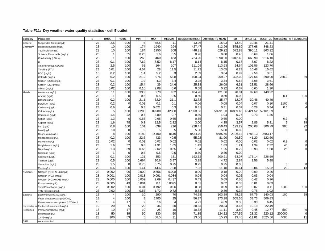
Table F11: Dry weather water quality statistics - cell 5 outlet
Category Parameter N RMDL %>DL MIN MAX MEDIAN GEOMETRIC MEAN ARITHMETIC MEAN SD 95%CI -LL 95%CI -UL GUIDELINE % > GUIDELINEGeneral Suspended Solids (mg/L) 23 2.5 100 5 58.5 11 13.06 15.93 13.40 10.46 21.41Chemistry Dissolved Solids (mg/L) 23 10 100 174 1940 294 427.47 612.96 575.69 377.68 848.23
Total Solids (mg/L) 23 10 100 184 1950 308 448.81 629.22 572.83 395.11 863.32Solvents Extractable (mg/L) 23 1 35 0.25 1.6 0.5 0.76 0.88 0.46 0.69 1.06Conductivity (uS/cm) 23 1 100 268 3460 453 724.20 1090.00 1042.62 663.90 1516.10pH 23 0.1 100 7.62 8.52 8.17 8.14 8.15 0.18 8.07 8.22Alkalinity (mg/L CaCO3) 23 2.5 100 68 164 107 111.09 113.63 24.64 103.56 123.70Turbidity (FTU) 23 0.01 100 4.54 28 11.5 11.72 13.05 6.29 10.48 15.62BOD (mg/L) 16 0.2 100 1.4 5.2 3 2.89 3.04 0.97 2.56 3.51Chloride (mg/L) 23 0.2 100 21.2 976 56.8 108.04 259.27 322.09 127.64 390.90 250.0 39Carbon (DOC) (mg/L) 23 0.1 100 1.9 4.3 3.4 3.28 3.34 0.64 3.08 3.61Carbon (DIC) (mg/L) 23 0.2 100 15.4 39 24.6 25.38 26.09 6.31 23.51 28.66Silicon (mg/L) 23 0.02 100 0.16 2.08 0.6 0.68 0.92 0.67 0.65 1.20
Metals Aluminum (ug/L) 23 11 100 39.9 270 102 104.78 121.30 70.01 92.69 149.92Arsenic (ug/L) 23 1 0 0.5 0.5 0.5 0.50 0.50 0.00 0.1 100Barium (ug/L) 23 0.2 100 21.1 62.9 31.1 33.72 35.47 12.27 30.46 40.49Beryllium (ug/L) 23 0.2 0 0.01 0.1 0.1 0.06 0.08 0.04 0.07 0.10 1100 0Cadmium (ug/L) 23 0.6 4 0.3 0.621 0.3 0.31 0.31 0.07 0.29 0.34 0.5 4Calcium (ug/L) 23 5 100 30200 89900 42300 47893.38 50291.30 16809.65 43421.52 57161.09Chromium (ug/L) 23 1.4 22 0.7 3.89 0.7 0.89 1.04 0.77 0.73 1.36Cobalt (ug/L) 23 1.3 0 0.65 0.65 0.65 0.65 0.65 0.00 0.9 0Copper (ug/L) 23 1.6 78 0.8 12.5 2.82 3.00 4.35 3.57 2.89 5.81 5 39Iron (ug/L) 23 0.8 100 101 639 216 228.47 250.43 123.22 200.08 300.79 300 22Lead (ug/L) 23 10 0 5 5 5 5.00 5.00 0.00 5 0Magnesium (ug/L) 23 8 100 5180 14100 8640 8434.70 8685.65 2196.14 7788.13 9583.17Manganese (ug/L) 23 0.2 100 23.6 433 49.5 55.92 81.90 99.59 41.20 122.60Mercury (ug/L) 23 0.02 0 0.01 0.02 0.02 0.02 0.02 0.00 0.02 0.02 0.2 0Molybdenum (ug/L) 23 1.6 52 0.8 4.91 1.65 1.49 1.83 1.21 1.34 2.32 40 0Nickel (ug/L) 23 1.3 39 0.65 2.62 0.65 1.04 1.25 0.79 0.93 1.58 25 0Selenium (ug/L) 23 1 0 0.5 0.5 0.5 0.50 0.50 0.00Strontium (ug/L) 23 0.1 100 121 353 181 192.62 200.91 63.07 175.14 226.69Titanium (ug/L) 23 0.5 100 0.664 10.6 3.97 3.89 4.72 2.84 3.56 5.88Vanadium (ug/L) 23 1.5 0 0.75 0.75 0.75 0.75 0.75 0.00 6 0Zinc (ug/L) 23 0.6 100 1.41 44.6 7.58 7.52 11.18 10.61 6.84 15.52 20 13
Nutrients Nitrogen (NH3+NH4) (mg/L) 23 0.002 96 0.002 0.856 0.098 0.09 0.18 0.20 0.09 0.26Nitrogen (NO2) (mg/L) 23 0.001 100 0.018 0.091 0.034 0.04 0.04 0.02 0.03 0.04Nitrogen (NO2+NO3) (mg/L) 23 0.005 100 0.059 2.69 0.437 0.43 0.69 0.66 0.42 0.96Phosphate (mg/L) 23 0.005 43 0.001 0.1 0.0025 0.01 0.02 0.03 0.01 0.03Total Phosphorus (mg/L) 23 0.002 100 0.04 0.192 0.06 0.08 0.09 0.05 0.07 0.11 0.03 100TKN Nitrogen (mg/L) 23 0.02 100 0.56 1.72 0.72 0.84 0.89 0.34 0.75 1.02
Bacteria Escherichia coli (c/100mL) 18 4 100 10 290 70 74.38 103.89 78.23 67.75 140.03 100 39Fecal streptococcus (c/100mL) 18 4 100 9 1700 25 56.87 273.28 505.55 39.73 506.83Pseudomonas aeruginosa (c/100mL) 18 4 17 2 16 4 4.21 4.89 3.38 3.33 6.45
Herbicides an 2,4,6 -trichlorophenol (ng/L) 19 20 5 20 36 20 20.63 20.84 3.67 19.19 22.49Pesticides Pentachlorophenol (ng/L) 18 10 17 10 25 10 10.78 11.11 3.60 9.45 12.77 500 0
Dicamba (ng/L) 18 50 39 50 830 50 71.85 124.22 207.59 28.32 220.12 200000 02,4 -D (ng/L) 23 100 53 5 58.5 11 13.06 15.93 13.40 -11.81 2025.50 4000 11
PAH none detected

Table F12: Dry weather water quality statistics - Lake Ontario
Category Parameter N RMDL %>DL MIN MAX MEDIAN GEOMETRIC MEAN ARITHMETIC MEAN SD 95%CI -LL 95%CI -UL GUIDELINE % > GUIDELINE #>DL #>GUIDELINEGeneral Suspended Solids (mg/L) 14 2.5 29 1.25 24 1.25 2.68 5.84 8.29 1.50 10.18 4Chemistry Dissolved Solids (mg/L) 14 10 100 180 204 192 192.47 192.57 6.49 189.17 195.97 14
Total Solids (mg/L) 14 10 100 180 220 196 197.82 198.14 11.83 191.95 204.34 14Solvents Extractable (mg/L) 14 1 21 0.25 8.5 0.5 0.62 1.15 2.15 0.02 2.27 3Conductivity (uS/cm) 14 1 100 276 315 296 295.84 296.00 10.11 290.71 301.29 14pH 14 0.1 100 8.11 8.66 8.325 8.35 8.36 0.17 8.26 8.45 14Alkalinity (mg/L CaCO3) 14 2.5 100 86 95 92 91.97 92.00 2.24 90.83 93.17 14Turbidity (FTU) 14 0.01 100 0.24 13.9 0.775 1.41 3.65 4.87 1.09 6.20 14BOD (mg/L) 10 0.2 100 0.4 2.4 0.7 0.73 0.86 0.60 0.49 1.23 10Chloride (mg/L) 14 0.2 100 21 53.2 21.8 23.24 24.06 8.41 19.65 28.46 250.0 0 14 0Carbon (DOC) (mg/L) 14 0.1 100 1.8 3.3 1.9 2.04 2.06 0.39 1.86 2.27 14Carbon (DIC) (mg/L) 14 0.2 100 19 28 21.6 21.52 21.60 2.06 20.52 22.68 14Silicon (mg/L) 14 0.02 100 0.04 0.98 0.13 0.13 0.23 0.26 0.09 0.36 14
Metals Aluminum (ug/L) 14 11 71 5.5 82.1 19.1 19.29 30.79 28.98 15.61 45.97 10Arsenic (ug/L) 14 1 0 0.5 0.5 0.5 0.50 0.50 0.00 0.1 100 0 14Barium (ug/L) 14 0.2 100 0.23 26.6 21.35 15.58 20.10 6.02 16.94 23.25 14Beryllium (ug/L) 14 0.2 0 0.01 0.1 0.1 0.04 0.06 0.05 0.04 0.09 1100 0 0 0Cadmium (ug/L) 14 0.6 0 0.3 0.3 0.3 0.30 0.30 0.00 0.30 0.30 0.5 0 0 0Calcium (ug/L) 14 5 100 27400 35800 33500 32754.50 32835.71 2333.57 31613.34 34058.09 14Chromium (ug/L) 14 1.4 14 0.7 2.36 0.7 0.80 0.87 0.47 0.62 1.12 2Cobalt (ug/L) 14 1.3 0 0.65 0.65 0.65 0.65 0.65 0.00 0.9 0 0 0Copper (ug/L) 14 1.6 36 0.8 7.3 0.8 1.43 2.14 2.27 0.95 3.33 5 14 5 2Iron (ug/L) 14 0.8 100 5.29 170 29.6 28.55 53.71 59.00 22.81 84.62 300 0 14 0Lead (ug/L) 14 10 7 5 11.3 5 5.30 5.45 1.68 4.57 6.33 5 7 1 1Magnesium (ug/L) 14 8 100 7290 8850 8455 8369.35 8380.00 429.85 8154.84 8605.16 14Manganese (ug/L) 14 0.2 100 0.737 11.3 2.315 2.90 4.14 3.87 2.12 6.17 14Mercury (ug/L) 14 0.02 0 0.01 0.02 0.02 0.01 0.02 0.01 0.01 0.02 0.2 0 0 0Molybdenum (ug/L) 14 1.6 7 0.8 1.74 0.8 0.85 0.87 0.25 0.74 1.00 40 0 1 0Nickel (ug/L) 14 1.3 21 0.65 11.4 0.65 0.91 1.57 2.86 0.07 3.07 25 0 3 0Selenium (ug/L) 14 1 0 0.5 0.5 0.5 0.50 0.50 0.00 0Strontium (ug/L) 14 0.1 100 140 171 160.5 159.43 159.64 8.45 155.21 164.07 14Titanium (ug/L) 14 0.5 43 0.25 4.35 0.25 0.60 1.23 1.52 0.44 2.02 6Vanadium (ug/L) 14 1.5 0 0.75 0.75 0.75 0.75 0.75 0.00 6 0 0 0Zinc (ug/L) 14 0.6 79 0.3 22.5 1.0285 1.37 3.20 5.79 0.17 6.23 20 7 11 1
Nutrients Nitrogen (NH3+NH4) (mg/L) 14 0.002 86 0.002 0.168 0.03 0.02 0.05 0.05 0.02 0.08 12Nitrogen (NO2) (mg/L) 14 0.001 100 0.004 0.028 0.0115 0.01 0.01 0.01 0.01 0.02 14Nitrogen (NO2+NO3) (mg/L) 14 0.005 100 0.226 0.556 0.362 0.33 0.34 0.09 0.29 0.39 14Phosphate (mg/L) 14 0.005 7 0.001 0.006 0.0025 0.00 0.00 0.00 0.00 0.00 1Total Phosphorus (mg/L) 14 0.002 100 0.008 0.056 0.012 0.01 0.02 0.01 0.01 0.02 0.03 7 14 1TKN Nitrogen (mg/L) 14 0.02 100 0.2 0.4 0.27 0.28 0.29 0.06 0.25 0.32 14
Bacteria Escherichia coli (c/100mL) 10 4 100 8 880 42 55.42 193.60 284.15 17.49 369.71 100 40 10 4Fecal streptococcus (c/100mL) 10 4 70 4 560 40 28.39 93.00 168.79 -11.61 197.61 7Pseudomonas aeruginosa (c/100mL) 10 4 10 2 50 4 3.90 7.80 14.86 -1.41 17.01 1
Herbicides and 2,4,6 -trichlorophenol (ng/L) 9 20 11 20 26 20 20.59 20.67 2.00 19.36 21.97 1Pesticides Pentachlorophenol (ng/L) 8 10 0 10 10 10 10.00 10.00 0.00 500 0 0 0
Dicamba (ng/L) 8 50 0 50 50 50 50.00 50.00 0.00 200000 0 0 02,4 -D (ng/L) 8 100 13 100 280 100 113.74 122.50 63.64 78.40 166.60 4000 0 1 0
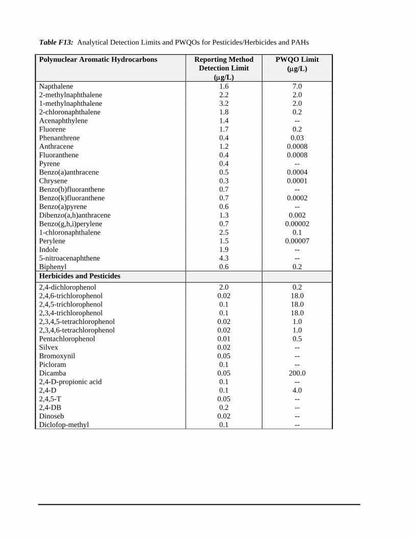
Table F13: Analytical Detection Limits and PWQOs for Pesticides/Herbicides and PAHs Polynuclear Aromatic Hydrocarbons Reporting Method
Detection Limit (g/L)
PWQO Limit (g/L)
Napthalene 1.6 7.0 2-methylnaphthalene 2.2 2.0 1-methylnaphthalene 3.2 2.0 2-chloronaphthalene 1.8 0.2 Acenaphthylene 1.4 -- Fluorene 1.7 0.2 Phenanthrene 0.4 0.03 Anthracene 1.2 0.0008 Fluoranthene 0.4 0.0008 Pyrene 0.4 -- Benzo(a)anthracene 0.5 0.0004 Chrysene 0.3 0.0001 Benzo(b)fluoranthene 0.7 -- Benzo(k)fluoranthene 0.7 0.0002 Benzo(a)pyrene 0.6 -- Dibenzo(a,h)anthracene 1.3 0.002 Benzo(g,h,i)perylene 0.7 0.00002 1-chloronaphthalene 2.5 0.1 Perylene 1.5 0.00007 Indole 1.9 -- 5-nitroacenaphthene 4.3 -- Biphenyl 0.6 0.2 Herbicides and Pesticides 2,4-dichlorophenol 2.0 0.2 2,4,6-trichlorophenol 0.02 18.0 2,4,5-trichlorophenol 0.1 18.0 2,3,4-trichlorophenol 0.1 18.0 2,3,4,5-tetrachlorophenol 0.02 1.0 2,3,4,6-tetrachlorophenol 0.02 1.0 Pentachlorophenol 0.01 0.5 Silvex 0.02 -- Bromoxynil 0.05 -- Picloram 0.1 -- Dicamba 0.05 200.0 2,4-D-propionic acid 0.1 -- 2,4-D 0.1 4.0 2,4,5-T 0.05 -- 2,4-DB 0.2 -- Dinoseb 0.02 -- Diclofop-methyl 0.1 --

APPENDIX G
Water Temperature Data

Figure G1 : Temperature fluctuations (upper graph: July 1 to September 16, 2000), durations and frequencies (lower graph: July 13 to Aug 9, 2000).
10
15
20
25
3001
/07/
00 0
0:00
11/0
7/00
00:
00
21/0
7/00
00:
00
31/0
7/00
00:
00
10/0
8/00
00:
00
20/0
8/00
00:
00
30/0
8/00
00:
00
09/0
9/00
00:
00
Tem
pera
ture
(deg
rees
Cel
sius
)
Inlet Cell 3 Cell 5
inlet data notavailable
cell 5 data not available cell 3 data not
available
0
50
100
150
200
250
300
12.1-13
13.1-14
14.1-15
15.1-16
16.1-17
17.1-18
18.1-19
19.1-20
20.1-21
21.1-22
22.1-23
23.1-24
24.1-25
25.1-26
26.1-27
27.1-28
28.1-29
29.1-30
Temperature range (degrees Celsius)
dura
tion
(hou
rs)
0
5
10
15
20
25
30
35
40
45
Freq
uenc
y (%
)
inletcell 3 outletcell 5 outlet
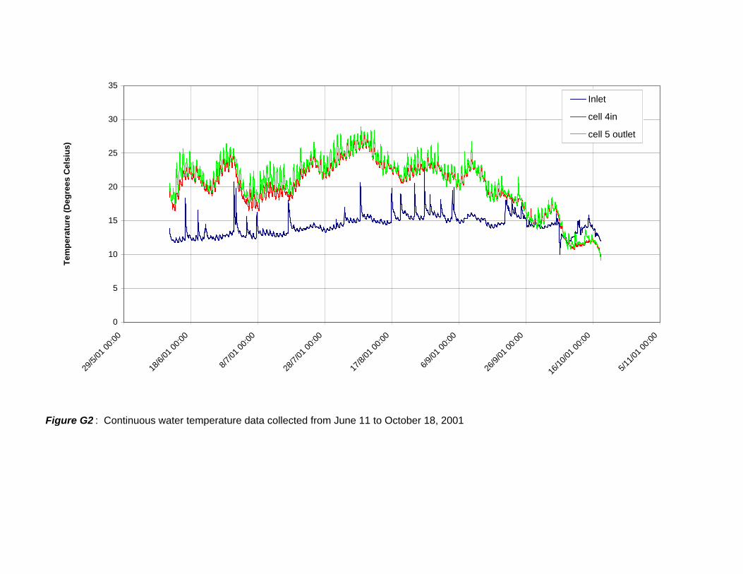
Figure G2 : Continuous water temperature data collected from June 11 to October 18, 2001
0
5
10
15
20
25
30
35
29/5/
01 00
:00
18/6/
01 00
:00
8/7/01
00:00
28/7/
01 00
:00
17/8/
01 00
:00
6/9/01
00:00
26/9/
01 00
:00
16/10
/01 00
:00
5/11/0
1 00:0
0
Tem
pera
ture
(Deg
rees
Cel
sius
)
Inlet
cell 4in
cell 5 outlet

Figure G3 : Water temperature measured on the south side of the cell 1-2 curtain at three depths below the water surface (0.5, 1.5 and 2.5 m)
June 12 - 30, 2002
14
16
18
20
22
24
26
28
6/6/2002 0:00 6/11/2002 0:00 6/16/2002 0:00 6/21/2002 0:00 6/26/2002 0:00 7/1/2002 0:00
Wat
er T
empe
ratu
re (D
egre
es C
elsi
us)
top middle bottom
July 2002
19
21
23
25
27
29
31
6/30/2002 0:00 7/5/2002 0:00 7/10/2002 0:00 7/15/2002 0:00 7/20/2002 0:00 7/25/2002 0:00 7/30/2002 0:00
Wat
er T
empe
ratu
re (D
egre
es C
elsi
us)
top middle bottom
August 2002
19
21
23
25
27
29
31
8/1/2002 0:14 8/6/2002 0:14 8/11/2002 0:14 8/16/2002 0:14 8/21/2002 0:14 8/26/2002 0:14 8/31/2002 0:14
Tem
pera
ture
(Deg
rees
Cel
sius
)
top middle bottom

APPENDIX H
Sediment Quality and Particle Size Distributions


0
10
20
30
40
50
60
70
80
90
100
0.1 1 10 100 1000Particle Size [um]
Perc
enta
ge G
reat
er T
han
[%]
Lake Ontario - A
Cell 1 - A
Cell 3 - A
Cell 4- A
Cell 5 - A
Lake Ontario Control - A
Lake Ontario - B
Cell 1 - B
Cell 3 - B
Cell 4 -B
Cell 5 - B
Lake Ontario Control - B
Lake Ontario C
Cell 1 - C
Cell 3 - C
Cell 4 - C
Cell 5 - C
Lake Ontario Control - C
Figure H2: Sediment particle size distributions

APPENDIX I
Removal Efficiencies (2000 monitoring season)
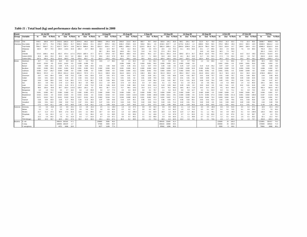
Table I1 : Total load (kg) and performance data for events monitored in 2000
EventGroup Variable In Out % Rem. In Out % Rem. In Out % Rem. In Out % Rem. In Out % Rem. In Out % Rem. In Out % Rem. In Out % Rem. In Out % Rem. In Out % Rem. In Out % Rem. In Out % Rem.
General TSS 4448.7 560.9 87.4 3410.3 1952.9 42.7 2544.3 446.2 82.5 4089.6 245.9 94.0 1459.9 212.9 85.4 683.7 35.7 94.8 833.8 145.1 82.6 395.1 159.1 59.7 212.5 42.7 79.9 243.8 16.3 93.3 77.0 10.3 86.6 18398.7 3828.0 79.2Chemistry Diss.Solids 3017.4 5377.1 -78.2 2798.2 5363.2 -91.7 6835.3 5259.4 23.1 2254.7 3070.2 -36.2 3236.2 2749.5 15.0 540.8 556.1 -2.8 2216.6 2237.7 -1.0 2175.8 2145.0 1.4 1699.8 739.5 56.5 470.0 595.0 -26.6 223.3 320.5 -43.5 25468.0 28413.2 -11.6
Total Solids 7504.7 5918.7 21.1 6237.7 7287.0 -16.8 9417.6 5686.6 39.6 6332.3 3310.1 47.7 4696.1 2956.3 37.0 1224.5 591.8 51.7 3061.0 2385.4 22.1 2565.8 2298.9 10.4 1913.9 786.3 58.9 715.0 610.0 14.7 299.9 330.9 -10.3 43968.3 32162.0 26.9Oil/grease 164.4 38.7 76.5 204.0 116.6 42.9 180.4 23.7 86.8 36.0 12.0 66.7 73.0 12.2 83.3 30.6 0.6 97.9 10.6 2.6 75.0 41.1 20.5 50.0 15.1 1.7 88.6 19.0 2.5 86.8 7.8 0.9 88.0 781.8 232.1 70.3BOD 88.7 36.0 59.5 143.6 40.1 72.0 12.8 3.6 72.0 57.0 25.3 55.6 24.8 4.0 83.8 34.5 7.5 78.3 361.3 116.5 67.7Chloride 572.5 1056.1 -84.5 402.2 874.4 -117.4 1762.0 1097.4 37.7 427.0 570.9 -33.7 803.0 458.0 43.0 104.6 90.3 13.7 521.4 391.6 24.9 509.0 327.4 35.7 481.8 112.6 76.6 97.0 103.0 -6.2 44.0 61.0 -38.5 5724.6 5142.8 10.2Carbon (DOC) 92.8 69.6 25.0 93.3 93.3 0.0 288.6 65.5 77.3 69.6 43.2 37.9 90.0 37.7 58.1 23.7 7.1 69.9 52.8 40.6 23.0 44.1 36.2 18.0 21.7 9.5 56.5 17.3 7.0 59.4 16.9 3.9 76.7 810.8 413.6 49.0Carbon (DIC) 297.9 545.4 -83.1 314.8 565.5 -79.6 478.5 454.7 5.0 191.9 278.2 -45.0 214.1 256.1 -19.6 50.0 55.6 -11.2 160.4 216.4 -34.9 143.7 219.1 -52.5 102.4 80.6 21.2 44.0 63.0 -43.2 19.2 30.6 -59.1 2016.9 2765.3 -37.1
Metals Aluminum 19.7 2.1 89.4 16.0 8.9 44.5 16.2 3.3 79.8 15.8 1.7 89.2 9.0 1.5 83.3 4.0 0.3 93.1 5.5 0.9 83.1 3.3 0.7 78.5 1.2 0.4 69.0 1.2 0.1 90.6 0.7 0.1 88.0 92.5 19.9 78.5Arsenic 0.010 0.010 0.0 0.015 0.015 0.0 0.009 0.009 0.0 0.006 0.006 0.0 0.003 0.001 50.0 0.005 0.005 0.0 0.005 0.005 0.0 0.001 0.001 0.0 0.001 0.001 50.0 0.055 0.053 3.3Barium 0.90 0.68 25.1 0.68 0.75 -11.2 0.99 0.66 33.0 0.61 0.36 40.9 0.46 0.35 24.2 0.14 0.07 47.8 0.30 0.32 -6.6 0.25 0.27 -11.0 0.15 0.10 35.2 0.07 0.07 3.3 0.04 0.04 0.3 4.60 3.68 19.9Beryllium 0.002 0.000 90.0 0.002 0.001 36.9 0.001 0.000 81.5 0.002 0.000 93.2 0.001 0.000 82.2 0.000 0.000 83.0 0.000 0.000 77.7 0.000 0.000 62.8 0.000 0.000 70.5 0.000 0.000 74.0 0.000 0.000 74.2 0.009 0.002 76.7Cadmium 0.006 0.017 -191.7 0.009 0.009 0.0 0.006 0.006 0.0 0.004 0.004 0.0 0.004 0.005 -32.1 0.003 0.001 75.6 0.003 0.003 0.0 0.003 0.003 0.0 0.001 0.001 0.0 0.001 0.001 0.0 0.000 0.000 0.0 0.039 0.049 -25.5Calcium 864.6 874.3 -1.1 655.8 1011.4 -54.2 1012.0 737.6 27.1 611.6 438.9 28.2 514.6 424.6 17.5 138.3 88.0 36.3 321.9 333.8 -3.7 290.4 319.7 -10.1 216.8 129.4 40.3 81.3 94.5 -16.3 33.4 50.9 -52.3 4740.8 4503.2 5.0Chromium 0.07 0.01 80.4 0.08 0.02 75.5 0.08 0.01 83.9 0.07 0.01 87.1 0.04 0.01 76.7 0.02 0.00 91.1 0.02 0.01 68.8 0.04 0.01 80.7 0.01 0.00 70.7 0.01 0.00 78.7 0.01 0.00 86.4 0.44 0.09 80.6Cobalt 0.03 0.01 62.6 0.02 0.02 0.0 0.03 0.01 51.9 0.03 0.01 71.1 0.01 0.01 0.0 0.01 0.00 70.0 0.01 0.01 0.0 0.01 0.01 0.0 0.00 0.00 0.0 0.00 0.00 50.8 0.00 0.00 52.9 0.14 0.08 43.0Copper 0.56 0.06 88.6 0.46 0.14 69.2 0.73 0.10 86.1 0.29 0.06 80.5 0.39 0.03 92.0 0.13 0.00 96.4 0.18 0.02 88.7 0.14 0.01 92.0 0.08 0.02 79.4 0.05 0.01 79.3 0.04 0.01 82.2 3.06 0.47 84.7Iron 28.2 5.8 79.5 17.8 11.3 36.3 40.3 8.6 78.8 21.2 3.4 84.0 17.6 3.4 81.0 9.4 0.7 93.0 9.1 2.1 76.4 5.2 2.0 61.3 2.0 0.8 59.1 1.9 0.3 86.6 1.4 0.2 85.9 154.1 38.5 75.0Lead 0.52 0.10 81.3 0.45 0.15 67.3 0.37 0.09 74.2 0.33 0.06 81.8 0.19 0.06 68.2 0.16 0.01 91.9 0.16 0.05 66.0 0.05 0.05 0.0 0.02 0.02 0.0 0.01 0.01 0.0 0.01 0.01 64.8 2.26 0.61 73.0Magnesium 99.8 158.6 -58.9 69.7 150.4 -115.9 130.8 130.2 0.5 66.6 80.7 -21.3 74.7 96.6 -29.3 19.4 21.5 -11.2 43.9 79.2 -80.3 38.6 66.3 -71.8 34.5 25.3 26.5 9.5 16.0 -69.0 4.3 7.8 -82.8 591.6 832.6 -40.7Manganese 6.4 1.8 72.3 3.3 2.7 18.2 5.6 1.9 65.8 3.0 0.7 77.3 2.5 0.4 82.8 0.6 0.1 78.7 1.1 0.4 61.5 0.6 0.5 12.7 0.2 0.1 42.3 0.3 0.1 71.1 0.2 0.0 73.2 23.8 8.8 62.9Mercury 0.001 0.000 85.7 0.000 0.000 0.0 0.002 0.000 87.5 0.000 0.000 75.0 0.000 0.000 0.0 0.000 0.000 75.0 0.000 0.000 0.0 0.000 0.000 0.0 0.000 0.000 0.0 0.000 0.000 0.0 0.000 0.000 66.7 0.004 0.001 70.7Molybdenum 0.015 0.015 0.0 0.023 0.023 0.0 0.015 0.015 0.0 0.010 0.010 0.0 0.010 0.022 -122.8 0.002 0.006 -185.0 0.008 0.011 -29.1 0.008 0.008 0.0 0.173 0.005 97.3 0.002 0.006 -211.3 0.001 0.002 -180.0 0.267 0.123 53.8Nickel 0.071 0.013 82.2 0.041 0.019 53.9 0.077 0.012 84.0 0.063 0.016 74.1 0.046 0.008 82.8 0.021 0.002 92.2 0.024 0.007 71.1 0.016 0.007 59.4 0.016 0.004 75.4 0.009 0.002 82.4 0.006 0.002 66.3 0.391 0.091 76.7Titanium 0.26 0.04 83.9 0.29 0.17 40.6 0.20 0.15 26.0 0.07 0.04 39.8 0.16 0.07 60.1 0.06 0.01 77.4 0.06 0.03 47.1 0.08 0.02 69.1 0.03 0.02 53.4 0.02 0.00 79.6 0.01 0.00 60.8 1.25 0.56 54.7Vanadium 0.08 0.01 82.0 0.08 0.02 73.2 0.07 0.01 80.9 0.07 0.01 87.0 0.04 0.01 75.6 0.02 0.00 91.6 0.03 0.01 71.4 0.03 0.01 70.1 0.00 0.00 0.0 0.01 0.00 69.9 0.00 0.00 76.6 0.43 0.09 78.8Zinc 2.71 0.24 91.1 1.88 0.57 69.8 2.35 0.16 93.2 1.31 0.08 93.9 1.29 0.07 94.8 0.57 0.01 97.5 0.58 0.06 89.6 0.45 0.04 90.9 0.20 0.02 90.6 0.15 0.01 94.0 0.11 0.01 93.1 11.60 1.26 89.1
Nutrients Ammonia 2.5 3.6 -43.8 4.3 6.6 -54.1 2.3 3.8 -62.3 2.5 3.1 -26.0 1.9 1.0 47.5 0.8 0.5 33.3 0.8 0.6 30.6 1.1 1.9 -61.2 0.3 0.5 -68.8 0.9 0.4 52.9 0.4 0.2 37.2 18.0 22.3 -24.2Nitrites 3.4 3.3 1.1 3.9 1.9 52.6 3.8 0.8 78.1 2.8 0.5 82.6 0.2 0.2 5.2 0.6 0.2 68.7 1.1 0.2 82.3 1.0 0.3 74.3 0.2 0.1 45.7 0.4 0.1 74.5 0.1 0.0 59.0 17.5 7.6 56.4Nitrates 21.7 11.4 47.3 30.9 17.8 42.3 13.6 4.2 69.0 19.7 3.5 82.3 1.0 3.2 -209.4 2.4 0.4 82.8 18.9 1.3 92.9 12.0 1.7 86.2 5.1 1.1 78.1 0.6 0.9 -35.9 0.1 0.4 -239.0 126.0 46.0 63.5Phosphate 2.4 0.4 82.4 1.2 1.1 2.5 0.8 0.1 89.4 0.9 0.1 89.5 0.0 0.0 65.6 0.1 0.1 43.6 1.3 0.0 97.9 0.7 0.1 82.0 0.1 0.0 80.6 0.2 0.0 87.6 0.4 0.0 99.7 8.0 2.0 75.1TP 12.2 1.9 84.2 7.8 4.5 41.8 9.3 1.7 81.8 6.7 0.9 87.1 4.6 0.7 85.2 2.1 0.3 86.6 4.4 0.8 82.6 2.1 1.1 48.8 0.7 0.2 77.7 1.2 0.1 91.0 1.0 0.1 93.2 52.1 12.2 76.7TKN Nitrogen 48.0 19.3 59.7 42.0 26.2 37.5 53.2 16.3 69.3 32.1 10.6 67.2 26.3 8.2 69.0 8.8 2.1 75.6 16.9 6.3 62.5 10.3 9.3 9.0 8.1 2.1 73.6 4.9 1.7 66.3 3.4 1.0 70.7 253.8 103.2 59.3
Bacteria E. coli 495516 262332 47.1 239860 8395 96.5 369425 31665 91.4 115000 25 100.0 1219801 302417 75.2F.strep. 169058 166144 1.7 57566 9355 83.8 348315 18999 94.5 105000 25 100.0 679940 194522 71.4P. aeruginosa 4372 3498 20.0 5277 1199 77.3 55942 2296 95.9 5250 5 99.9 70841 6998 90.1
14-Jul-00 22-Sep-00 4-Oct-00 27-Oct-0023-Aug-00 2-Sep-00 10-Sep-00 14-Sep-00 TOTAL30-Jul-00 8-Aug-0017-Jul-00