Embed Size (px)
Citation preview
Trade-off Balancing in Scheduling for Flow ShopProduction and Perioperative Processes
Wei (Mike) LiUniversity of Kentucky, Lexington, Kentucky, USA
Barrie R. Nault(corresponding author)
University of Calgary, Calgary, Alberta, Canada
Honghan YeUniversity of Wisconsin, Madison, Wisconsin, USA
We balance trade-offs between two fundamental and possibly inconsistent objectives, minimization of max-
imum completion time and minimization of total completion time, in scheduling serial processes. We use a
novel approach of current and future deviations (CFD) to model the trade-offs between the two completion
times. We also use weights α and β to balance trade-offs at the operation level and at the process level,
respectively. Accordingly, we develop a constructive CFD heuristic, and compare its performance with three
leading constructive heuristics in scheduling based on three separate datasets: 5400 small-scale instances, 120
Taillard’s benchmark instances, and one-year historical records of operating room scheduling in a university
hospital system. We show that minimization of maximum completion time and minimization of total com-
pletion time yield inconsistent scheduling sequences, and the two sequences are relatively uncorrelated. We
also show that our CFD heuristic can balance trade-offs between these two objectives, outperform the three
leading heuristics across different performance measures, and allow larger variations on two fundamental
completion times. This means that trade-off balancing by our CFD heuristic enables a serial process to have
a larger tolerance on variations of process performance, and keeps the process better under control. This
performance improvement can be significant for flow shop scheduling in manufacturing in trading-off pro-
duction and holding costs, and for operating room scheduling across the perioperative process in healthcare
in trading-off hospital cost and patient waiting time.
Version: August 25, 2018
Keywords : Flow Shop Production, Perioperative Process, Scheduling, Trade-off Balancing.
1. Introduction
A serial process consists of a number of stages, workstations, machines, and/or operations
that process jobs sequentially from the first to the last (Pinedo 2008). Typical examples of
serial processes are a flow line with m machines for production scheduling in manufacturing
1
Li, Nault and Ye: Trade-off Balancing in Serial Process Scheduling2
systems, and a 3-stage perioperative (periop) process for operating room (OR) scheduling
in healthcare systems, with preoperative (preop), intraoperative (intraop), and postopera-
tive (postop) stages (Ye et al. 2017, Gupta and Denton 2008). Maximum completion time
(Cmax) and total completion time (∑Cj) are two fundamental performance measures in
serial processes. Given an n-job m-machine instance, Cmax =Cn,m is the completion time
of the last job n on the last machine m, and∑Cj =
∑nj=1Cj,m is the sum of completion
times of all j = 1, ..., n jobs on the last machine m. Flow time or average completion time
(C) equals∑Cj/n, and thus for a fixed n, min(
∑Cj) is the same as min(C).
Minimizations of these two completion times, min(Cmax) and min(∑Cj), drive many
other performance metrics. For example, in production scheduling, utilization (Util) equals
to the workload divided by a working period, where the workload is the sum of processing
times and the working period is the difference between maximum completion time and
start time. Given due dates of all jobs, dj for j = 1, ..., n, tardiness is defined as Tj =
max{Cj − dj; 0}, and earliness is defined as Ej = max{dj −Cj; 0} in T’kindt and Billaut
(2002). Accordingly, maximum tardiness (max(Tj)) or maximum earliness (max(Ej)) may
relate to Cmax, and total tardiness (∑Tj) or total earliness (
∑Ej) may relate to
∑Cj
(Slowinski 1981, Kim 1995, Figueira et al. 2010). Work-in-process (WIP ) inventory levels
are influenced by the difference of average completion times between two adjacent machines
or stages. In OR scheduling, overtime is evaluated by the difference between maximum
completion time and OR block time; cost to the hospital can be a function of utilization of
the periop process; and length of stay (LoS) across the periop process and post-anesthesia
care unit (PACU) staffing are related to patient flow time (PtF ).
Although Cmax is included in∑Cj, it is difficult to seek optimal solutions to min(Cmax)
and to min(∑Cj) because they areNP -complete problems for scheduling in a serial process
with m> 2 (Garey et al. 1976, Hoogeveen and Kawaguchi 1999). In practice, heuristics
and simple priority dispatching rules (PDRs) are used to achieve simple objectives and to
seek near optimal solutions to real scheduling problems. For example, in OR scheduling,
the shortest processing time (SPT) rule is recommended to smooth patient flow across the
periop process, even over a genetic algorithm (Gul et al. 2011), and the longest processing
time (LPT) rule is recommended to improve OR utilization (Magerlein and Martin 1978).
In flow shop production scheduling, the NEH heuristic (Nawaz et al. 1983) is commonly
regarded as the best constructive heuristic in the world to min(Cmax), based on which
Li, Nault and Ye: Trade-off Balancing in Serial Process Scheduling3
heuristics are developed to improve utilization and to reduce CO2 emission (Gahm et al.
2016, Fang et al. 2011, Ding et al. 2016). In contrast, the LR heuristic (Liu and Reeves 2001)
and the FF heuristic (Fernandez-Viagas and Framinan 2015) are regarded as two of the
best constructive heuristics to min(∑Cj). However, two questions are left for operations
management, given the inconsistency between min(Cmax) and min(∑Cj) (Li et al. 2014).
One question is whether near optimal solutions to simple objectives can balance the trade-
offs (TO) between metrics based on Cmax and metrics based on∑Cj, and the other is
whether the process is better under control if operations management focus on trade-off
balancing instead on optimizing single objectives.
In this work, we develop and test a new heuristic that we name the current and future
deviation (CFD) heuristic for sequencing/scheduling in a serial process with m machines
or stages. The development of our CFD heuristic combines two underlying ideas. First,
we use one set of weights to address two coupled deviations generated by one completion
time from both upper and lower bounds as fundamental elements of the heuristic. Second,
we employ another set of weights to balance trade-offs between results from two well-
understood objectives: min(Cmax) and min(∑Cj). Following the traditional notation in
flow shop scheduling (T’kindt and Billaut 2002), we deal with a bi-criteria scheduling
problem for an m-machine permutation (prmu) flow shop with a linear function (Fl) of
two scheduling objectives of Cmax and∑Cj, F |prmu|Fl(Cmax,
∑Cj).
Two objectives of min(Cmax) and min(∑Cj) are inconsistent with each other (Li et al.
2014), which means one completion time of a job j on a machine i, Cj,i, may minimize the
deviation to one objective, but maximize the deviation to the other. Consequently in our
CFD heuristic, we first factorize the two coupled deviations, and use weights α to construct
an initial sequence. We then explicitly recognize the inconsistency between the results of
min(Cmax) and min(∑Cj), and use weights β in a linear trade-off function to reconstruct
the initial sequence. Although both α and β are weights and can change separately, α is
applied to fundamental elements of two coupled deviations at the operation level, and β is
applied to performance at the process level. Through case studies in Section 4, preferences
for trade-off balancing should be consistent at the both levels, which means α= β.
Three separate datasets are used to test the performance of our CFD heuristic. The first
dataset consists of randomly generated small-scale instances where optimal sequences can
be found for min(Cmax), min(∑Cj) and min(TO). The second dataset is classic Taillard’s
Li, Nault and Ye: Trade-off Balancing in Serial Process Scheduling4
benchmarks for flow shop scheduling (Taillard 1993). The third dataset consists historical
records of nearly 30,000 patient cases from 2013-14 in OR scheduling across the three-stage
periop process at University of Kentucky HealthCare (UKHC). Compared to NEH, LR and
FF, we find that our CFD heuristic clearly outperforms all on min(Cmax), min(∑Cj) and
min(TO) for the dataset of small-scale instances, outperforms them for Taillard’s bench-
marks on min(Cmax) and min(TO), but marginally on min(∑Cj) especially compared to
FF, and dominates all for our UKHC dataset. In addition, using process control metrics
we show that our CFD heuristic yields a process that is better under control than the
historical data from UKHC. Finally, we compute Spearman rank order correlations among
the sequences for min(Cmax), min(∑Cj) and min(TO) for each dataset, finding that they
are close to zero and empirically support the inconsistency between each pair of objectives.
Thus, our three main contributions are first developing a novel CFD heuristic that
uses decoupled deviations from bounds and allows for trade-offs between objectives like
min(Cmax) and min(∑Cj), second showing that the CFD heuristic outperforms three lead-
ing alternative constructive heuristics based on a series of empirical tests across generated,
benchmark, and real historical datasets, and third keeping serial processes better under
control based on trade-off balancing.
The rest of this paper is organized as follows. A brief literature review is provided in
Section 2, the programming logic and steps of our CFD heuristic are illustrated in Section
3, results of empirical case studies are analyzed in Section 4, and conclusion and future
work are drawn in Section 5.
2. Literature Review
The literatures on production scheduling and on trade-off balancing (or multi-objective
optimization) are vast. In this section, we provide brief reviews in these two areas from
the perspective of heuristic development. For further details about prior research, refer to
Pinedo (2008) and T’kindt and Billaut (2002) for flow shop scheduling, and to Malakooti
(2013) and Slowinski and Weglarz (1989) for trade-off balancing.
2.1. Flow Shop Scheduling
Balancing trade-offs between min(Cmax) and min(∑Cj) is still a fundamental challenge
to scheduling in serial processes, especially with different objectives in operations man-
agement, and given Garey et al. (1976) proved that min(Cmax) is NP -complete for a flow
Li, Nault and Ye: Trade-off Balancing in Serial Process Scheduling5
line with m > 3, and Hoogeveen and Kawaguchi (1999) proved that min(∑Cj) is NP -
complete for a flow line with m> 2. Research on flow shop scheduling has been carried out
for more than 6 decades since the classic Johnson’s algorithm in Johnson (1954). During
the first two decades, research on flow shop scheduling focused on seeking optimal solu-
tions by using optimization and branch & bound techniques (Gupta and Stafford 2006).
However, the emergence of NP -completeness theory in the third decade (1975−1984) pro-
foundly influenced the direction of research on flow shop scheduling, changing to seek
near optimal solutions by using heuristics. Initially, min(Cmax) was the primary scheduling
objective for permutation flow shop production. During the fourth decade (1985−1994),
hybrid flow shop production emerged and many artificial intelligence (AI) based heuris-
tics were developed. The fifth decade (1995−2004) witnessed the proliferation of various
flow shop problems, objectives, and solution approaches. Current research on flow shop
scheduling (2005−present) has extended to sustainability (Gahm et al. 2016) in terms of
energy-efficiency, water usage, CO2 emission (Ding et al. 2016, Fang et al. 2011, Zhang
et al. 2014), which intensifies the necessity of trade-off balancing.
Framinan et al. (2004) proposed a general framework for heuristic development consisting
of three phases: index development (generating an initial sequence), solution construction
(changing the initial sequence based on some inserting schemes), and solution improvement
(changing the job sequence based on AI). PDRs are typical examples in phase one. The
NEH heuristic proposed by Nawaz, Enscore, and Ham (Nawaz et al. 1983) and the LR
heuristic proposed by Liu and Reeves (2001) are typical examples in phase two that also
spillover to phase three. As we indicated above, the NEH, LR and FF heuristics are the
best of constructive heuristics to min(Cmax) and min(∑Cj), respectively (Kalczynski and
Kamburowski 2007, Ruiz and Maroto 2005, Fernandez-Viagas and Framinan 2015). Meta-
heuristics, such as genetic algorithms, neural networks, and simulated annealing, are typical
examples in phase three. Scheduling methods developed in the first two phases can facilitate
heuristic development in phase three. In general, there is a trade-off between solution
quality and computational complexity or computation time in choosing a heuristic for a
scheduling problem. At one extreme, the solution quality of PDRs is low, but they provide
a solution fast, saving time in decision making, and they are used in the other two phases
of heuristic development. At the other extreme, the solution quality of meta-heuristics is
Li, Nault and Ye: Trade-off Balancing in Serial Process Scheduling6
high, but it is time consuming to get a solution by using them (Ruiz and Maroto 2005).
Our CFD heuristic proceeds through the first two phases of heuristic development above.
As we compare our CFD heuristic to the best of the best constructive heuristics in our
empirical case studies, we briefly describe the key sequencing logics of the NEH, LR and
FF heuristics. The LPT rule is used as an index function in the NEH heuristic to generate
an initial sequence of n jobs. The first two jobs in the initial sequence are enumerated for
a better partial solution to min(Cmax). As j = 3, ..., n for each of the rest n− 2 jobs in the
initial sequence, job j is inserted into j possible positions in the intermediate sequence,
and one of j partial sequences with min(Cmax) is selected for the next round of iteration
until j = n. The computational complexity of the NEH heuristic originally was O(n3m),
and was improved by Taillard (1990) to O(n2m) for n-job m-machine permutation flow
shop problems to min(Cmax).
In the index development phase of the LR heuristic, an initial sequence is constructed
based on an index function with the sum of two terms, weighted total idle times (IT ) and
artificial total flow times (AT ). Afterwards, each of a number of x jobs is selected as the
first job in the initial sequence and sequence reconstruction based on the above mentioned
index function occurs, generating a number of x candidate LR(x) sequences, where x =
1, ..., n. Local search techniques of both forward pairwise exchanging (FPE) and backward
pairwise exchanging (BPE) are then applied to x reconstructed sequences to improve the
solution quality of LR(x) on min(∑Cj). The computational complexity is O(n3m) for
LR(1) without local search, and O(n4m) for LR(n) with local search. Based on Taillard’s
benchmarks (Taillard 1993), LR(n) outperformed six of other heuristics to min(∑Cj) (Liu
and Reeves 2001), including the Ho (1995) heuristic. Based on computational complexities
in the same order, we compare our CFD heuristic to the NEH with the original settings
and to the LR(1) without local search.
Similar to the LR heuristic, Fernandez-Viagas and Framinan (2015) also use AT and
IT to construct a job sequence to min(∑Cj). Their novel approach integrates two tuning
parameters in the FF heuristic, specifically a parameter a in calculating AT ′ and another
parameter b in calculating IT ′, by which the computational complexity of FF is reduced
to O(n2m). After tuning the two parameters, the FF heuristic with a= 4 and b= 1 out-
performs the LR heuristic on average for Taillard’s benchmarks.
Li, Nault and Ye: Trade-off Balancing in Serial Process Scheduling7
2.2. Trade-off Balancing
Without loss of generality, a multi-objective combinatorial optimization (MOCO) problem
with a number of q = 1, ...,O minimization objectives can be defined as follows (Czyzak
and Jaszkiewics 1998), min{z1 = f1(x), z2 = f2(x), ..., zO = fO(x)}, subject to x∈ F , where
the solution x is a vector of discrete decision variables and F is the set of feasible solutions.
Czyzak and Jaszkiewics (1998) explicitly pointed out two factors which cause difficulties
in solving MOCO problems. The first is that intensive cooperation with decision makers
(DMs) should be involved in seeking solutions, which requires efficient solutions generated
by effective tools. The second is that an MOCO problem is more difficult to solve, if each
problem of single-objective versions is NP -hard. “Priori” and “posteriori” approaches are
widely used in seeking and evaluating solutions to MOCO problems, respectively (Ciavotta
et al. 2013). A linear function with weights is a typical example of the “priori” approach,
that is, z =∑O
q=1 βqzq with∑O
q=1 βq = 1. For example, Framinan et al. (2002) developed
a bi-objective heuristic to minimize the weighted sum of Cmax and∑Cj, and the NEH
insertion method was applied. In this heuristic, a function TO= β · n2·Cmax +(1−β) ·
∑Cj
was developed, where β is the weight on Cmax, and an unscheduled job j with minimum
TO is selected and attached to the current partial sequence. Pareto efficiency is a typical
example of the “posteriori” approach. A solution x ∈ F is Pareto efficient, if and only if
there is no x′ ∈ F such that ∀q fq(x′)≤ fq(x) and ∃q fq(x′)< fq(x). Linear functions with
weights as in the “priori” approach usually have metrics measured in different scales, and
it is difficult to map βq into valid preferences of DMs (Ciavotta et al. 2013).
Czyzak and Jaszkiewics (1998) proposed two quality metrics that respectively measure
the average and maximum deviations between the set F and a reference set R, which can
be used to address such a problem in the “priori” approach. Given y ∈ R, the deviation
defined in Czyzak and Jaszkiewics (1998) is dq(x,y) = max{0, [fq(y)− fq(x)]/[fMAXq (R)−
fMINq (R)]}, where fMAX
q (R) and fMINq (R) are the maximum and minimum values of func-
tion fq in the reference set R, respectively. Therefore, [fq(y)−fq(x)]/[fMAXq (R)−fMIN
q (R)]
is a normalized deviation. Based on normalized deviations of dq(x,y), the first metric is
defined as D1R = 1|R|∑
y∈R minx∈F{dq(x,y)}, where |R| is the cardinality of set R. The
second metric is defined as D2R = maxy∈R{minx∈F{dq(x,y)}}. D1R measures the average
deviations with equal weights of 1|R| , and D2R measures the maximum deviation from the
reference set. Moreover, Czyzak and Jaszkiewics (1998) pointed out that the lower the
Li, Nault and Ye: Trade-off Balancing in Serial Process Scheduling8
ratio D2R/D1R, the more uniform the distribution of solutions from the set F over the set
R. However, DMs should be cautious in using the ratio of D2R/D1R to evaluate heuristics.
A reason will be provided in Section 4.1 based on our case studies. Framinan (2009) and
Ishibuchi et al. (2003) developed different metaheuristics by using the D1R metric, but with
a slight modification, in which the deviation is measured by d(x,y) =√∑
(f ∗q (y)− f ∗q (x))2,
and f ∗q (·) = [fq(·)− fMINq (R)]/[fMAX
q (R)− fMINq (R)].
As we will see in the following sections, two underlying ideas characterize our CFD
heuristic in trade-off balancing. Firstly, we operate on two coupled deviations and use α
to decouple them at the operation level. Secondly, we use normalization not only on two
coupled deviations at the operation level, but also on performances of Cmax and∑Cj
at the process level, and use β to address preferences on normalized performances. The
magnitudes of Cmax and∑Cj are not the same, which is the reason why Framinan (2009)
used β · n2
to address this concern, but we use normalizations accordingly. Normalized Cmax
and∑Cj are dimensionless, and provide accurate values to our TO function for trade-
off balancing. Consequently, our CFD heuristic outperforms the NEH and LR heuristics
respectively on min(Cmax), min(∑Cj), and min(TO), whereas Framinan et al.’s heuristic
outperforms other heuristics in their case studies only on min(TO), but does not outper-
form the NEH heuristic on min(Cmax), nor the Ho (1995) heuristic on min(∑Cj).
Trade-offs should be balanced not only at the system level, but also at the process and
operation levels. We note that decision making on trade-off balancing only at the system
level is not effective. For example, the economic order quantity (EOQ) model proposed
by Harris in 1913, reprinted in Harris 1990, has been widely applied to balance trade-offs
between production cost and holding cost at the system level. Based on the EOQ model,
many other models have been developed for ordering in different situations, such as the
newsvendor model (Stevenson 2009) and (Q,r) model (Hopp and Spearman 2000). These
trade-off-based models are often embedded in software developed for manufacturing and
services, such as ERP and MRP-II systems (Hopp and Spearman 2000, Orlicky 1975). As
a result, WIP inventory levels are still high in manufacturing systems (GeneralElectric
2014), and waiting times for a surgery are still long in healthcare systems (AHRQ 2013).
In our CFD heuristic, weights α balance trade-offs at the operation level for each job on
each machine, and weights β balance trade-offs at the process level for the performance of
a whole serial process.
Li, Nault and Ye: Trade-off Balancing in Serial Process Scheduling9
3. A Current and Future Deviations Heuristic
In this section, we first address the concept of deviation from bounds (DB) at the operation
level, which are the reference values of lower and upper bounds of completion times, denoted
as OLCj,i and OUCj,i, and by using which we model the two coupled deviations and
develop an index function with α to generate an initial sequence in phase one of index
development. Second, we address the lower and upper bounds of completion times at the
process level, denoted as PLCj,i and PUCj,i, deviations from which are used in phase two
of solution construction. Third, we address how we model trade-offs at the process level
by using β to reconstruct the initial sequence to obtain a final sequence.
3.1. Two Coupled Deviations for Trade-offs as Initial Sequence
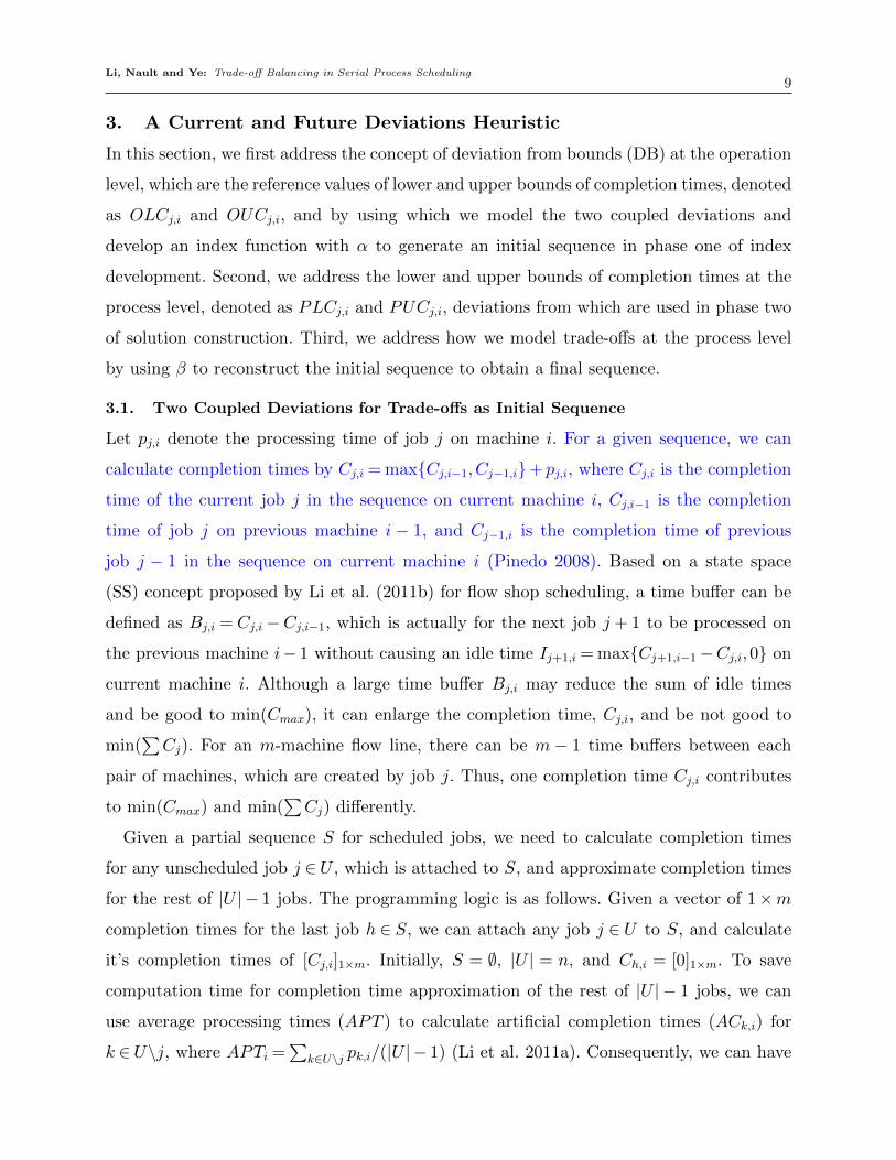
Let pj,i denote the processing time of job j on machine i. For a given sequence, we can
calculate completion times by Cj,i = max{Cj,i−1,Cj−1,i}+ pj,i, where Cj,i is the completion
time of the current job j in the sequence on current machine i, Cj,i−1 is the completion
time of job j on previous machine i − 1, and Cj−1,i is the completion time of previous
job j − 1 in the sequence on current machine i (Pinedo 2008). Based on a state space
(SS) concept proposed by Li et al. (2011b) for flow shop scheduling, a time buffer can be
defined as Bj,i = Cj,i −Cj,i−1, which is actually for the next job j + 1 to be processed on
the previous machine i− 1 without causing an idle time Ij+1,i = max{Cj+1,i−1−Cj,i,0} on
current machine i. Although a large time buffer Bj,i may reduce the sum of idle times
and be good to min(Cmax), it can enlarge the completion time, Cj,i, and be not good to
min(∑Cj). For an m-machine flow line, there can be m− 1 time buffers between each
pair of machines, which are created by job j. Thus, one completion time Cj,i contributes
to min(Cmax) and min(∑Cj) differently.
Given a partial sequence S for scheduled jobs, we need to calculate completion times
for any unscheduled job j ∈U , which is attached to S, and approximate completion times
for the rest of |U | − 1 jobs. The programming logic is as follows. Given a vector of 1×m
completion times for the last job h ∈ S, we can attach any job j ∈ U to S, and calculate
it’s completion times of [Cj,i]1×m. Initially, S = ∅, |U | = n, and Ch,i = [0]1×m. To save
computation time for completion time approximation of the rest of |U | − 1 jobs, we can
use average processing times (APT ) to calculate artificial completion times (ACk,i) for
k ∈U\j, where APTi =∑
k∈U\j pk,i/(|U | − 1) (Li et al. 2011a). Consequently, we can have
Li, Nault and Ye: Trade-off Balancing in Serial Process Scheduling10
a three-dimensional matrix of[CU
j,i
]|U |×m×|U |, where each element in the third dimension
represents a |U | ×m matrix of completion times by attaching a job j ∈ U to S. Based on
the third dimension of[CU
j,i
], the reference values for lower and upper bounds of completion
times at the operation level for each job j on each machine i are calculated as,
OLCj,i = minj∈U{CU
j,i} for i= 1, ...,m,
OUCj,i = maxj∈U{CU
j,i} for i= 1, ...,m.(1)
Given[CU
j,i
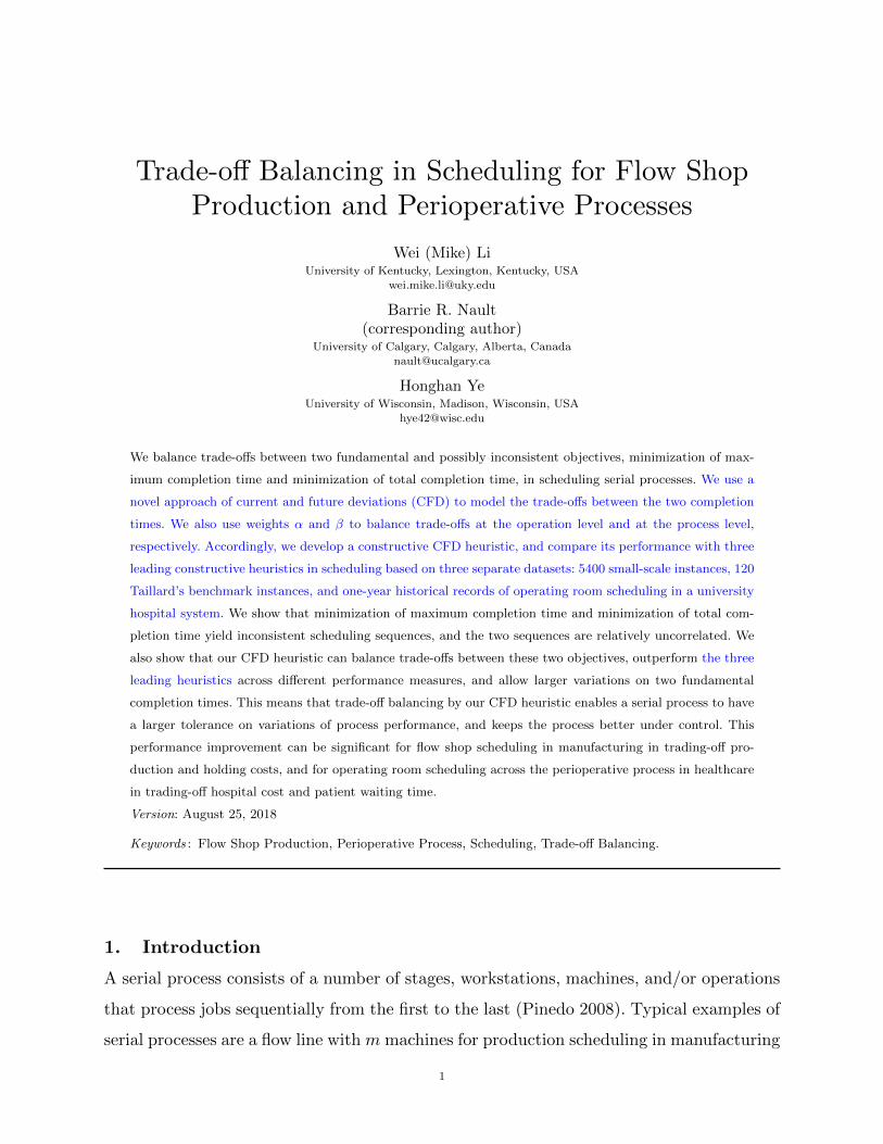
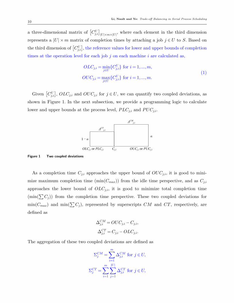
], OLCj,i and OUCj,i for j ∈ U , we can quantify two coupled deviations, as
shown in Figure 1. In the next subsection, we provide a programming logic to calculate
lower and upper bounds at the process level, PLCj,i and PUCj,i.
M1
M2
p1,1 p2,1 pj,1 pj+1,1
I1,2 p1,2 I2,2 p2,2 Ij,2 pj,2 Ij+1,2 pj+1,2
pn,1
pn,2In,2
OLCj,i or PLCj,i Cj,i
ΔCTj,i
ΔCMj,i
α 1–α
E(CM) CM & CT
α
ΔCM
E(CT)
ΔCT
1–α
Obj1
Obj2
1
1
0 0.5
0.5
R
S
O
OUCj,i or PUCj,i
Figure 1 Two coupled deviations
As a completion time Cj,i approaches the upper bound of OUCj,i, it is good to mini-
mize maximum completion time (min(Cmax)) from the idle time perspective, and as Cj,i
approaches the lower bound of OLCj,i, it is good to minimize total completion time
(min(∑Cj)) from the completion time perspective. These two coupled deviations for
min(Cmax) and min(∑Cj), represented by superscripts CM and CT , respectively, are
defined as
∆CMj,i =OUCj,i−Cj,i,
∆CTj,i =Cj,i−OLCj,i.
The aggregation of these two coupled deviations are defined as
ΣCMj =
m∑i=1
∆CMj,i for j ∈U,
ΣCTj =
m∑i=1
|U |∑j=1
∆CTj,i for j ∈U,
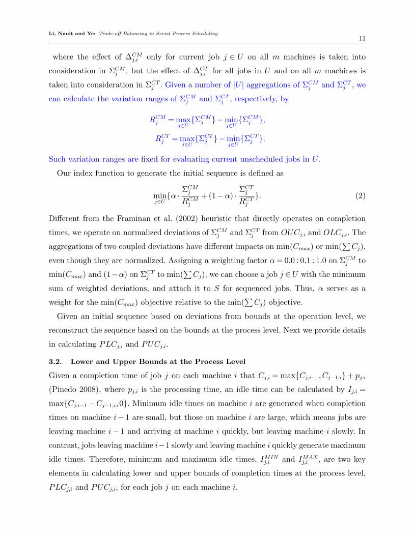
Li, Nault and Ye: Trade-off Balancing in Serial Process Scheduling11
where the effect of ∆CMj,i only for current job j ∈ U on all m machines is taken into
consideration in ΣCMj , but the effect of ∆CT
j,i for all jobs in U and on all m machines is
taken into consideration in ΣCTj . Given a number of |U | aggregations of ΣCM
j and ΣCTj , we
can calculate the variation ranges of ΣCMj and ΣCT
j , respectively, by
RCMj = max
j∈U{ΣCM
j }−minj∈U{ΣCM
j },
RCTj = max
j∈U{ΣCT
j }−minj∈U{ΣCT
j }.
Such variation ranges are fixed for evaluating current unscheduled jobs in U .
Our index function to generate the initial sequence is defined as
minj∈U{α ·
ΣCMj
RCMj
+ (1−α) ·ΣCT
j
RCTj
}. (2)
Different from the Framinan et al. (2002) heuristic that directly operates on completion
times, we operate on normalized deviations of ΣCMj and ΣCT
j from OUCj,i and OLCj,i. The
aggregations of two coupled deviations have different impacts on min(Cmax) or min(∑Cj),
even though they are normalized. Assigning a weighting factor α= 0.0 : 0.1 : 1.0 on ΣCMj to
min(Cmax) and (1−α) on ΣCTj to min(
∑Cj), we can choose a job j ∈U with the minimum
sum of weighted deviations, and attach it to S for sequenced jobs. Thus, α serves as a
weight for the min(Cmax) objective relative to the min(∑Cj) objective.
Given an initial sequence based on deviations from bounds at the operation level, we
reconstruct the sequence based on the bounds at the process level. Next we provide details
in calculating PLCj,i and PUCj,i.
3.2. Lower and Upper Bounds at the Process Level
Given a completion time of job j on each machine i that Cj,i = max{Cj,i−1,Cj−1,i}+ pj,i
(Pinedo 2008), where pj,i is the processing time, an idle time can be calculated by Ij,i =
max{Cj,i−1−Cj−1,i,0}. Minimum idle times on machine i are generated when completion
times on machine i− 1 are small, but those on machine i are large, which means jobs are
leaving machine i− 1 and arriving at machine i quickly, but leaving machine i slowly. In
contrast, jobs leaving machine i−1 slowly and leaving machine i quickly generate maximum
idle times. Therefore, minimum and maximum idle times, IMINj,i and IMAX
j,i , are two key
elements in calculating lower and upper bounds of completion times at the process level,
PLCj,i and PUCj,i, for each job j on each machine i.
Li, Nault and Ye: Trade-off Balancing in Serial Process Scheduling12
Processing times pj,i on each machine i = 1, ...,m can be sorted into two series. One
series of processing times is sorted by the LPT rule in a non-ascending order, recorded
as pLPTj,i , and the other is sorted by the SPT rule in a non-descending order, recorded as
pSPTj,i . Given the assumptions that all of n jobs are available to be processed on machine 1
at time zero, which means there is no idle times on machine 1 so IMINj,1 = 0 and IMAX
j,1 = 0,
we calculate PLCj,i and PUCj,i as follows:
IMINj,i = max{PLCj,i−1−PUCj−1,i,0}
= max{(PLCj−1,i−1 + IMINj,i−1 + pSPT
j,i−1)− (PUCj−2,i + IMAXj−1,i + pLPT
j−1,i),0},(3)
IMAXj,i = max{PUCj,i−1−PLCj−1,i,0}
= max{(PUCj−1,i−1 + IMAXj,i−1 + pLPT
j,i−1)− (PLCj−2,i + IMINj−1,i + pSPT
j−1,i),0},(4)
and thus
PLCj,i = PLCj−1,i + IMINj,i + pSPT
j,i and PUCj,i = PUCj−1,i + IMAXj,i + pLPT
j,i . (5)
3.3. An Evaluation Function for Trade-offs in Sequence Reconstruction
After generating an initial sequence based on (2), we reconstruct the sequence based on
the following scheme to address trade-offs between output variables at a production line
or process level. Our trade-off function to finalize a sequence is defined as
minr=1,...,j
{β · Cj,m−PLC1,m
PUCj,m−PLC1,m
+ (1−β) ·∑j
k=1(Ck,m−PLCk,m)∑jk=1(PUCk,m−PLCk,m)
}, (6)
where r represents a possible position of job j in the partial sequence of S ∪{j}, and β =
0.0 : 0.1 : 1.0 represents a preference for min(Cmax) relative to min(∑Cj). The optimization
in (6) evaluates output deviations on the last machinem and from the lower bounds of PLC
for both min(Cmax) and min(∑Cj). Different from calculation at the operation level, the
deviation for min(Cmax) on machine m is based on the difference between the completion
time for current job j and the lower bound for job 1, and the deviation for min(∑Cj) is
only for current j jobs in S. This scheme can be extended to evaluate output deviations
on any machine or stage, depending on management concerns.
Similar to the NEH heuristic, we enumerate the first two jobs in the initial sequence,
and get a partial sequence S with a better value in (6). As j = 3, ..., n for the remaining
jobs, we put job j into r = 1, ..., j possible positions of the partial sequence S, and based
on the minimum value of (6), we can finalize a sequence for trade-off balancing.
Li, Nault and Ye: Trade-off Balancing in Serial Process Scheduling13
The computational complexity of this sequence reconstruction is O(n3m). Therefore,
the overall computational complexity of CFD is O(n3m). Allowing for the weights given
to min(Cmax) and min(∑Cj) to differ in the generation of an initial sequence (α) and in
the sequence reconstruction (β) provides additional flexibility in trade-off balancing in our
CFD heuristic.
3.4. Programming Logic and Pseudocode
The programming logic and steps of our CFD heuristic are summarized as follows.
Step 0. Initialization, [P ]n×m for processing times, S for scheduled jobs, which can be
empty initially, U for unscheduled jobs, which can be {1, ..., n} initially, lower and upper
bounds of completion times at the process level, PLCj,i and PUCj,i, which are sequence
independent, according to (3), (4), and (5).
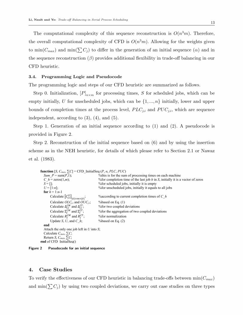
Step 1. Generation of an initial sequence according to (1) and (2). A pseudocode is
provided in Figure 2.
Step 2. Reconstruction of the initial sequence based on (6) and by using the insertion
scheme as in the NEH heuristic, for details of which please refer to Section 2.1 or Nawaz
et al. (1983).
function [S, Cmax, ∑C] = CFD_InitialSeq (P, α, PLC, PUC) Sum_P = sum(P,1); %this is for the sum of processing times on each machine C_h = zeros(1,m); %for completion time of the last job h in S, initially it is a vector of zeros S = []; %for scheduled jobs, initially it is empty U = [1:n]; %for unscheduled jobs, initially it equals to all jobs for h = 1:n-1
Calculate , | | | |; %according to current completion times of C_h
Calculate OLCj,i and OUCj,i; %based on Eq. (1) Calculate ∆ , and ∆ , ; %for two coupled deviations Calculate Σ and Σ ; %for the aggregation of two coupled deviations Calculate and ; %for normalization Update S, U, and C_h; %based on Eq. (2)
end Attach the only one job left in U into S; Calculate Cmax, ∑C; Return S, Cmax, ∑C;
end of CFD_InitialSeq()
Figure 2 Pseudocode for an initial sequence
4. Case Studies
To verify the effectiveness of our CFD heuristic in balancing trade-offs between min(Cmax)
and min(∑Cj) by using two coupled deviations, we carry out case studies on three types
Li, Nault and Ye: Trade-off Balancing in Serial Process Scheduling14
of data: small-scale instances, Taillard’s benchmarks, and historical OR data from the
University of Kentucky HealthCare (UKHC). We present the results respectively for each
type of data, and then we discuss the empirical relationships among different sequences to
min(Cmax), min(∑Cj) and min(TO) which we define in (9) below, generated by our CFD
heuristic using different weights.
4.1. 5400 Small-Scale Instances
For small-scale instances, the number of jobs ranges from n= 5, ...,10, yielding six options,
and the number of machines is set at m= 2 · (i+ 1) for i= 1, ...,9, yielding nine options
ranging from 5 to 20. For each of the resulting 54 combinations, 100 instances are randomly
generated, and the processing times follow a uniform distribution between [1,99]. Therefore,
there are 5400 small-scale instances in total.
Because the number of jobs is relatively small, n ≤ 10, we can use an enumeration
method to find the best (or minimum) and worst (or maximum) solutions to min(Cmax)
and min(∑Cj) as references R. Given best and worst values of fMIN
q,k and fMAXq,k for each
instance k and for each objective q, with q= 1 for min(Cmax) and q= 2 for min(∑Cj), we
can define a normalized deviation (ND) as follows,
NDq,k(H,R) =fq,k(H)− fMIN
q,k (R)
fMAXq,k (R)− fMIN
q,k (R)· 100, (7)
where fq,k(H) is the solution generated by a scheduling method H. This NDq,k(H,R) is
normalized in the same way as dq(x,y) defined in Czyzak and Jaszkiewics (1998). Similarly,
Fernandez-Viagas and Framinan (2015) defined a relative percentage deviation (RPD) as
RPDq,k(H,R) = [fq,k(H)− fMINq,k (R)]/fMIN
q,k (R) · 100. Accordingly, an average normalized
deviation (AND) is defined as follows,
ANDq(H,R) =1
K
K∑k=1
NDq,k(H,R), (8)
where K is the number of instances.
Based on ANDq for each objective, our trade-off function is defined as follows,
TO(H,R) = β ·AND1(H,R) + (1−β) ·AND2(H,R). (9)
This evaluation metric for trade-off balancing is similar to but different from the D1R
metric defined in the literature. First, TO(H,R) flexibly integrates DMs’ preferences into
Li, Nault and Ye: Trade-off Balancing in Serial Process Scheduling15
the evaluation, by changing weights β on min(Cmax), not by equal weights as defined in
Czyzak and Jaszkiewics (1998). Second, TO(H,R) actually is the expected value of trade-
off balancing, not a standard deviation, as a squared root of the sum of squared differences
defined in Ishibuchi et al. (2003).
Given α= β in (2) and (6), our CFD(α) heuristic generates 11 sequences, each of which
has [AND1,AND2] values. The comparison between the CFD(α), NEH, LR, and FF
heuristics is shown in Table 1 based on TO values defined in (9) for all 5400 small-scale
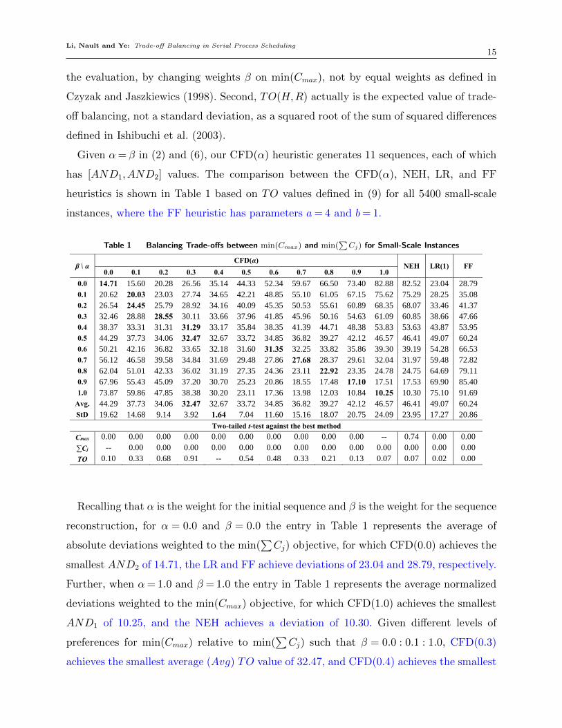
instances, where the FF heuristic has parameters a= 4 and b= 1.
Table 1 Balancing Trade-offs between min(Cmax) and min(∑Cj) for Small-Scale Instances
Table 1 Trade-off Values of Cmax and ∑Cj with Different Preferences for Small-Scale Instances
β \ α CFD(α)
NEH LR(1) FF 0.0 0.1 0.2 0.3 0.4 0.5 0.6 0.7 0.8 0.9 1.0
0.0 14.71 15.60 20.28 26.56 35.14 44.33 52.34 59.67 66.50 73.40 82.88 82.52 23.04 28.79 0.1 20.62 20.03 23.03 27.74 34.65 42.21 48.85 55.10 61.05 67.15 75.62 75.29 28.25 35.08 0.2 26.54 24.45 25.79 28.92 34.16 40.09 45.35 50.53 55.61 60.89 68.35 68.07 33.46 41.37 0.3 32.46 28.88 28.55 30.11 33.66 37.96 41.85 45.96 50.16 54.63 61.09 60.85 38.66 47.66 0.4 38.37 33.31 31.31 31.29 33.17 35.84 38.35 41.39 44.71 48.38 53.83 53.63 43.87 53.95 0.5 44.29 37.73 34.06 32.47 32.67 33.72 34.85 36.82 39.27 42.12 46.57 46.41 49.07 60.24 0.6 50.21 42.16 36.82 33.65 32.18 31.60 31.35 32.25 33.82 35.86 39.30 39.19 54.28 66.53 0.7 56.12 46.58 39.58 34.84 31.69 29.48 27.86 27.68 28.37 29.61 32.04 31.97 59.48 72.82 0.8 62.04 51.01 42.33 36.02 31.19 27.35 24.36 23.11 22.92 23.35 24.78 24.75 64.69 79.11 0.9 67.96 55.43 45.09 37.20 30.70 25.23 20.86 18.55 17.48 17.10 17.51 17.53 69.90 85.40 1.0 73.87 59.86 47.85 38.38 30.20 23.11 17.36 13.98 12.03 10.84 10.25 10.30 75.10 91.69
Avg. 44.29 37.73 34.06 32.47 32.67 33.72 34.85 36.82 39.27 42.12 46.57 46.41 49.07 60.24 StD 19.62 14.68 9.14 3.92 1.64 7.04 11.60 15.16 18.07 20.75 24.09 23.95 17.27 20.86
Two-tailed t-test against the best method
Cmax 0.00 0.00 0.00 0.00 0.00 0.00 0.00 0.00 0.00 0.00 -- 0.74 0.00 0.00 ∑Cj -- 0.00 0.00 0.00 0.00 0.00 0.00 0.00 0.00 0.00 0.00 0.00 0.00 0.00 TO 0.10 0.33 0.68 0.91 -- 0.54 0.48 0.33 0.21 0.13 0.07 0.07 0.02 0.00
Recalling that α is the weight for the initial sequence and β is the weight for the sequence
reconstruction, for α = 0.0 and β = 0.0 the entry in Table 1 represents the average of
absolute deviations weighted to the min(∑Cj) objective, for which CFD(0.0) achieves the
smallest AND2 of 14.71, the LR and FF achieve deviations of 23.04 and 28.79, respectively.
Further, when α= 1.0 and β = 1.0 the entry in Table 1 represents the average normalized
deviations weighted to the min(Cmax) objective, for which CFD(1.0) achieves the smallest
AND1 of 10.25, and the NEH achieves a deviation of 10.30. Given different levels of
preferences for min(Cmax) relative to min(∑Cj) such that β = 0.0 : 0.1 : 1.0, CFD(0.3)
achieves the smallest average (Avg) TO value of 32.47, and CFD(0.4) achieves the smallest
Li, Nault and Ye: Trade-off Balancing in Serial Process Scheduling16
standard deviation (StD) of 1.64. Notice that the LR heuristic generates smaller deviations
than the FF heuristic for all different levels of preferences β for small-scale instances.
For each of three objectives, a two-tailed t-test is carried out among the 14 sequencing
methods (NEH, LR, FF and 11 of CFD) against the best one on min(Cmax), min(∑Cj)
and min(TO) respectively, and the p-value is provided in Table 1. Given a 95% confidence
interval, we can tell from Table 1 that CFD(1.0) is not significantly different from the
NEH heuristic on min(Cmax), although it achieves a smaller AND1 value on min(Cmax).
CFD(0.0,0.1,0.2) heuristics are significantly different from the LR and FF heuristics
and achieve better average values on min(∑Cj) for small-scale instances. CFD(0.3) and
CFD(0.5) are not significantly different from each other on min(TO), but significantly
different from the LR and FF heuristics.
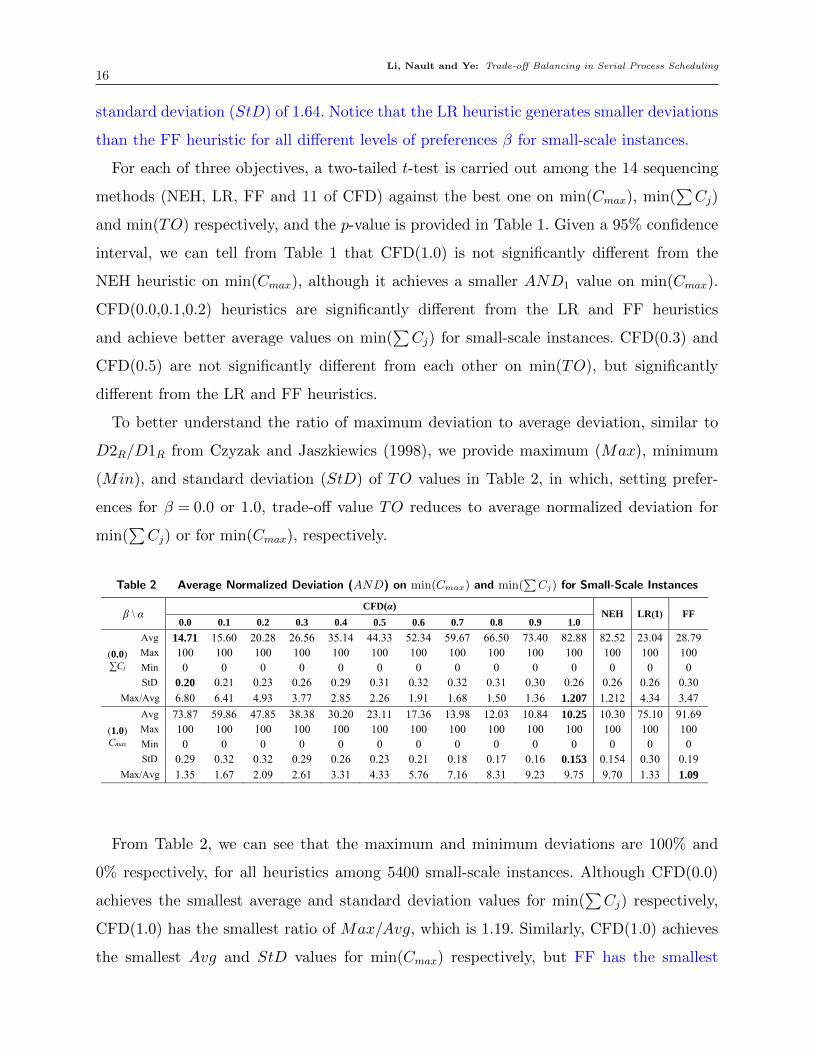
To better understand the ratio of maximum deviation to average deviation, similar to
D2R/D1R from Czyzak and Jaszkiewics (1998), we provide maximum (Max), minimum
(Min), and standard deviation (StD) of TO values in Table 2, in which, setting prefer-
ences for β = 0.0 or 1.0, trade-off value TO reduces to average normalized deviation for
min(∑Cj) or for min(Cmax), respectively.
Table 2 Average Normalized Deviation (AND) on min(Cmax) and min(∑Cj) for Small-Scale Instances
β \ α CFD(α)
NEH LR(1) FF 0.0 0.1 0.2 0.3 0.4 0.5 0.6 0.7 0.8 0.9 1.0
(0.0) ∑Cj
Avg 14.71 15.60 20.28 26.56 35.14 44.33 52.34 59.67 66.50 73.40 82.88 82.52 23.04 28.79 Max 100 100 100 100 100 100 100 100 100 100 100 100 100 100 Min 0 0 0 0 0 0 0 0 0 0 0 0 0 0 StD 0.20 0.21 0.23 0.26 0.29 0.31 0.32 0.32 0.31 0.30 0.26 0.26 0.26 0.30
Max/Avg 6.80 6.41 4.93 3.77 2.85 2.26 1.91 1.68 1.50 1.36 1.207 1.212 4.34 3.47
(1.0) Cmax
Avg 73.87 59.86 47.85 38.38 30.20 23.11 17.36 13.98 12.03 10.84 10.25 10.30 75.10 91.69 Max 100 100 100 100 100 100 100 100 100 100 100 100 100 100 Min 0 0 0 0 0 0 0 0 0 0 0 0 0 0 StD 0.29 0.32 0.32 0.29 0.26 0.23 0.21 0.18 0.17 0.16 0.153 0.154 0.30 0.19
Max/Avg 1.35 1.67 2.09 2.61 3.31 4.33 5.76 7.16 8.31 9.23 9.75 9.70 1.33 1.09
From Table 2, we can see that the maximum and minimum deviations are 100% and
0% respectively, for all heuristics among 5400 small-scale instances. Although CFD(0.0)
achieves the smallest average and standard deviation values for min(∑Cj) respectively,
CFD(1.0) has the smallest ratio of Max/Avg, which is 1.19. Similarly, CFD(1.0) achieves
the smallest Avg and StD values for min(Cmax) respectively, but FF has the smallest
Li, Nault and Ye: Trade-off Balancing in Serial Process Scheduling17
ratio of Max/Avg, which is 1.09. This result clearly shows that the distribution of per-
formance is more complex than can be evaluated simply by a ratio, and more statistically
robust methods such as statistical process control (SPC) techniques we use in the following
sections can be more reliable.
These results for small-scale instances, based on deviations from optimal solutions,
answer the first question of whether near optimal solutions to simple objectives can balance
the trade-offs. Based on a 2-tuple of [AND1(H,R),AND2(H,R)] that represent deviations
from optimal solutions for a given method q across min(Cmax) and min(∑Cj), [10.25,82.88]
for CFD(1.0) has a small deviation on min(Cmax) but a large deviation on min(∑Cj),
and [73.87,14.71] for CFD(0.0) has a large deviation on min(Cmax) but a small deviation
on min(∑Cj). Comparatively, [23.11,44.33] for CFD(0.5) is between those deviations for
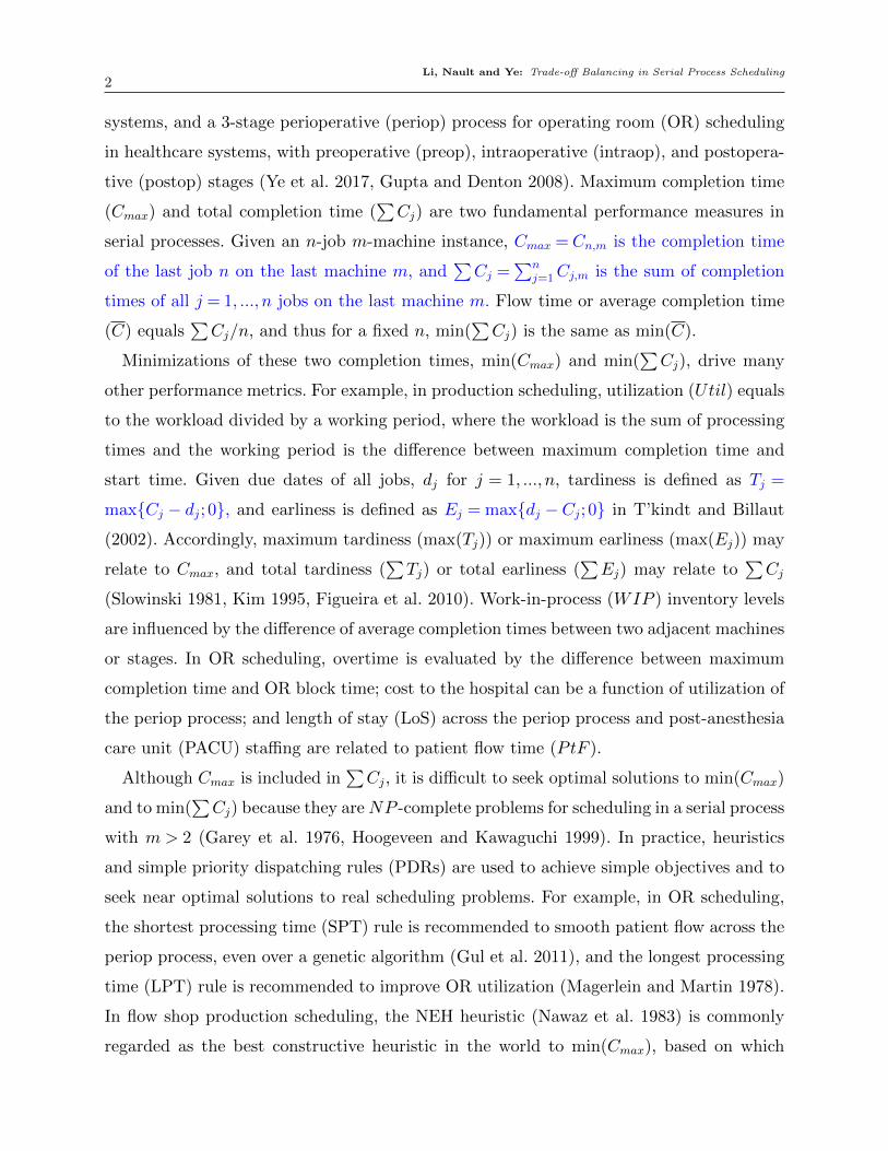
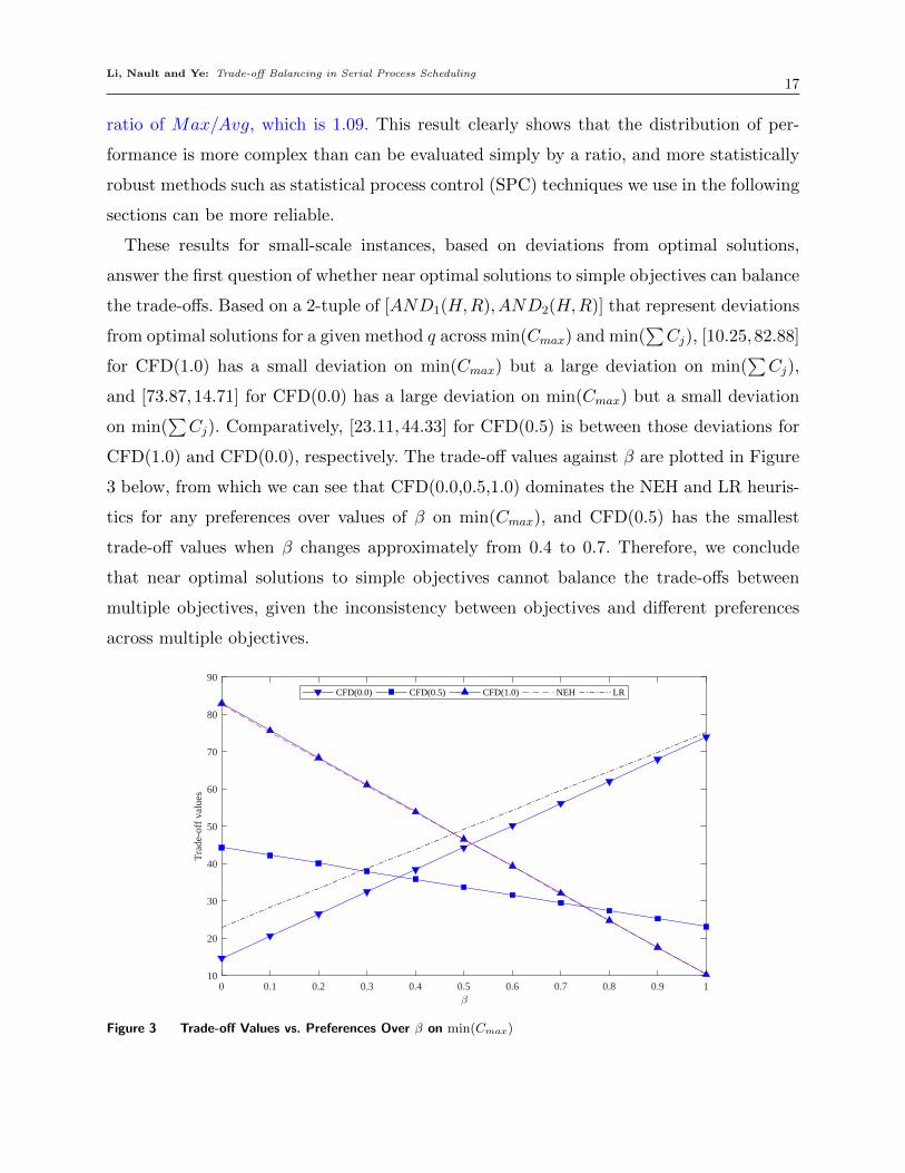
CFD(1.0) and CFD(0.0), respectively. The trade-off values against β are plotted in Figure
3 below, from which we can see that CFD(0.0,0.5,1.0) dominates the NEH and LR heuris-
tics for any preferences over values of β on min(Cmax), and CFD(0.5) has the smallest
trade-off values when β changes approximately from 0.4 to 0.7. Therefore, we conclude
that near optimal solutions to simple objectives cannot balance the trade-offs between
multiple objectives, given the inconsistency between objectives and different preferences
across multiple objectives.
0 0.1 0.2 0.3 0.4 0.5 0.6 0.7 0.8 0.9 110
20
30
40
50
60
70
80
90
Tra
de-o
ff v
alue
s
CFD(0.0) CFD(0.5) CFD(1.0) NEH LR
Figure 3 Trade-off Values vs. Preferences Over β on min(Cmax)
Li, Nault and Ye: Trade-off Balancing in Serial Process Scheduling18
4.2. 120 Instances in Taillard’s Benchmarks
Taillard’s benchmarks are classic in flow shop scheduling, and are commonly used to test
scheduling methods on min(Cmax) and on min(∑Cj). There are 12 scales in Taillard’s
benchmarks, ranging from a 20-job 5-machine flow line to a 500-job 20-machine flow line,
10 instances in each scale, and 120 instances in total.
Because min(Cmax) and min(∑Cj) are NP -complete problems, best known solutions
(B) are used to calculate normalized deviations, instead of using optimal solutions. B1 for
min(Cmax) can be found at http://mistic.heig-vd.ch/taillard/. B2 for min(∑Cj)
is the minimum between the FF results and those in Liu and Reeves (2001), in which
scheduling methods with high computational complexities are involved in generating B2,
such as meta-heuristics and LR(n) with FPE(n) and BPE(n). As maximization is involved
in this type of case studies on Taillard’s benchmarks, normalized deviations from best
solutions are calculated as follows,
NDq,k =|fq,k(H,R)−Bq,k(R)||Wq,k(R)−Bq,k(R)|
· 100,
where Wq,k(R) represents the worst solution for an instance k. If minimization is an objec-
tive, then Bq = minR fq(R) and Wq = maxR fq(R). Contrarily, if maximization is an objec-
tive, then Bq = maxR fq(R) and Wo = minR fq(R).
To compare our CFD heuristic with NEH, LR and FF, we calculate four other per-
formance measures in addition to min(Cmax) and min(∑Cj). The first is the average
utilization (Util) of a flow line, which relates to workload,∑pj, and maximum completion
time Cmax on each machine. The second is the average WIP inventory level (WIP -A),
which relates to∑Cj on each machine. The third is the sum of maximum WIP inventory
levels (WIP -MS), which means the overall holding capacity of m − 1 WIP inventories
in a flow line. The fourth is the maximum of max WIP inventory capacity (WIP -MM)
that indicates the maximum of m−1 WIP inventories, the location of which is meaningful
for operations management. Li and Freiheit (2016) provide details for calculating these
performance measures. The best and worst solutions on these four performance measures
are based on actual performance of the NEH, LR, and CFD(α) heuristics. The average
normalized deviations on each objective are provided in Table 3, for all 120 instances and
for the NEH, LR, FF, CFD(α) heuristics.
Li, Nault and Ye: Trade-off Balancing in Serial Process Scheduling19
Table 3 Average Normalized Deviations by CFD(α), NEH, LR and FF Heuristics for Taillard’s Benchmarks
Table 3 ARPD by CFD(α), NEH and LR(1) Heuristics for Taillard’s Benchmarks
Metrics CFD(α)
NEH LR(1) FF 0.0 0.1 0.2 0.3 0.4 0.5 0.6 0.7 0.8 0.9 1.0
Cmax 86.93 55.71 46.86 40.96 35.58 27.20 22.94 21.12 21.22 21.33 21.96 22.04 84.99 87.91 ∑Cj 20.78 22.11 25.16 31.43 40.60 59.42 68.83 75.83 78.64 85.17 86.77 87.90 22.59 19.88 Util 83.60 63.98 53.21 48.64 38.41 22.95 15.83 12.70 13.88 11.89 15.11 14.42 86.28 82.69 WIP-A 10.41 18.38 23.53 32.03 41.93 53.21 64.08 68.78 70.90 76.80 85.98 88.45 11.38 12.01
WIP-MS 6.95 11.45 13.52 17.82 23.04 26.07 30.33 31.48 32.94 36.58 43.27 45.24 15.65 6.96 WIP-MM 29.50 28.42 27.25 29.86 33.72 28.86 32.34 34.27 33.80 35.41 40.27 41.94 36.99 27.26
Two-tailed t-test against the best method Cmax 0.00 0.00 0.00 0.00 0.00 0.00 0.00 -- 0.88 0.77 0.20 0.20 0.00 0.00 ∑Cj 0.56 0.17 0.00 0.00 0.00 0.00 0.00 0.00 0.00 0.00 0.00 0.00 0.07 -- Util 0.00 0.00 0.00 0.00 0.00 0.00 0.02 0.58 0.14 -- 0.05 0.11 0.00 0.00 WIP-A -- 0.00 0.00 0.00 0.00 0.00 0.00 0.00 0.00 0.00 0.00 0.00 0.60 0.32
WIP-MS -- 0.00 0.00 0.00 0.00 0.00 0.00 0.00 0.00 0.00 0.00 0.00 0.00 0.00 WIP-MM 0.46 0.68 -- 0.32 0.05 0.63 0.09 0.04 0.06 0.01 0.00 0.00 0.01 0.01
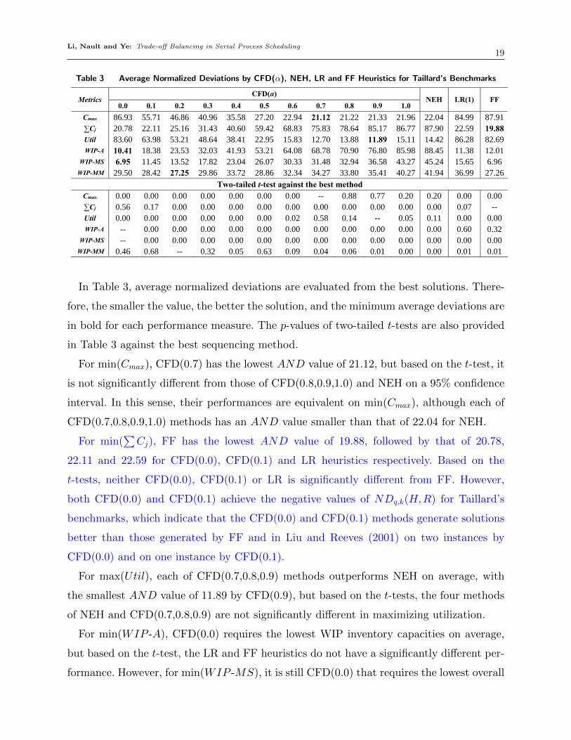
In Table 3, average normalized deviations are evaluated from the best solutions. There-
fore, the smaller the value, the better the solution, and the minimum average deviations are
in bold for each performance measure. The p-values of two-tailed t-tests are also provided
in Table 3 against the best sequencing method.
For min(Cmax), CFD(0.7) has the lowest AND value of 21.12, but based on the t-test, it
is not significantly different from those of CFD(0.8,0.9,1.0) and NEH on a 95% confidence
interval. In this sense, their performances are equivalent on min(Cmax), although each of
CFD(0.7,0.8,0.9,1.0) methods has an AND value smaller than that of 22.04 for NEH.
For min(∑Cj), FF has the lowest AND value of 19.88, followed by that of 20.78,
22.11 and 22.59 for CFD(0.0), CFD(0.1) and LR heuristics respectively. Based on the
t-tests, neither CFD(0.0), CFD(0.1) or LR is significantly different from FF. However,
both CFD(0.0) and CFD(0.1) achieve the negative values of NDq,k(H,R) for Taillard’s
benchmarks, which indicate that the CFD(0.0) and CFD(0.1) methods generate solutions
better than those generated by FF and in Liu and Reeves (2001) on two instances by
CFD(0.0) and on one instance by CFD(0.1).
For max(Util), each of CFD(0.7,0.8,0.9) methods outperforms NEH on average, with
the smallest AND value of 11.89 by CFD(0.9), but based on the t-tests, the four methods
of NEH and CFD(0.7,0.8,0.9) are not significantly different in maximizing utilization.
For min(WIP -A), CFD(0.0) requires the lowest WIP inventory capacities on average,
but based on the t-test, the LR and FF heuristics do not have a significantly different per-
formance. However, for min(WIP -MS), it is still CFD(0.0) that requires the lowest overall
Li, Nault and Ye: Trade-off Balancing in Serial Process Scheduling20
WIP inventory capacities across the process, but based on the t-test, it is significantly
lower than other heuristics.
Finally, for min(WIP -MM), CFD(0.2) requires the lowest maximum WIP inventory
capacity, and based on the t-test, CFD(0.0,0.1,0.2,0.3,0.4,0.5,0.6,0.8) are not significantly
different from each other.
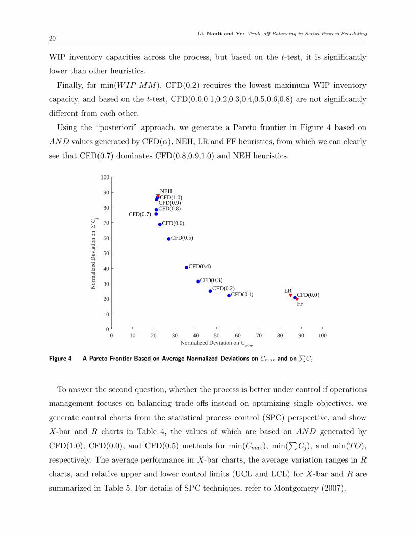
Using the “posteriori” approach, we generate a Pareto frontier in Figure 4 based on
AND values generated by CFD(α), NEH, LR and FF heuristics, from which we can clearly
see that CFD(0.7) dominates CFD(0.8,0.9,1.0) and NEH heuristics.
0 10 20 30 40 50 60 70 80 90 100Normalized Deviation on C
max
0
10
20
30
40
50
60
70
80
90
100
Nor
mal
ized
Dev
iatio
n on
C
j
CFD(0.0)CFD(0.1)CFD(0.2)
CFD(0.3)
CFD(0.4)
CFD(0.5)
CFD(0.6)
CFD(0.7)CFD(0.8)CFD(0.9)CFD(1.0)NEH
LR
FF
Figure 4 A Pareto Frontier Based on Average Normalized Deviations on Cmax and on∑Cj
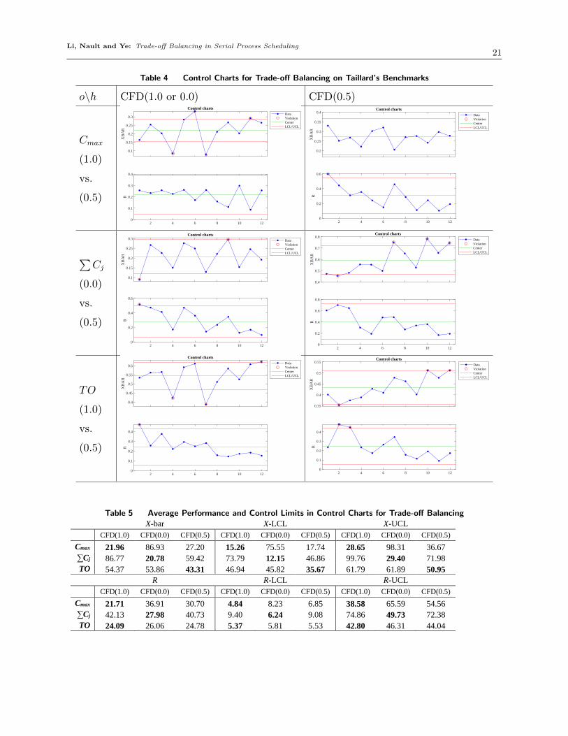
To answer the second question, whether the process is better under control if operations
management focuses on balancing trade-offs instead on optimizing single objectives, we
generate control charts from the statistical process control (SPC) perspective, and show
X-bar and R charts in Table 4, the values of which are based on AND generated by
CFD(1.0), CFD(0.0), and CFD(0.5) methods for min(Cmax), min(∑Cj), and min(TO),
respectively. The average performance in X-bar charts, the average variation ranges in R
charts, and relative upper and lower control limits (UCL and LCL) for X-bar and R are
summarized in Table 5. For details of SPC techniques, refer to Montgomery (2007).
Li, Nault and Ye: Trade-off Balancing in Serial Process Scheduling21
Table 4 Control Charts for Trade-off Balancing on Taillard’s Benchmarks
o\h CFD(1.0 or 0.0) CFD(0.5)
Cmax
(1.0)
vs.
(0.5)
0.1
0.15
0.2
0.25
0.3
XB
AR
Control chartsDataViolationCenterLCL/UCL
2 4 6 8 10 120
0.1
0.2
0.3
0.4
R
0.2
0.25
0.3
0.35
0.4
XB
AR
Control chartsDataViolationCenterLCL/UCL
2 4 6 8 10 120
0.2
0.4
0.6
R
∑Cj
(0.0)
vs.
(0.5)
0.1
0.15
0.2
0.25
0.3
XB
AR
Control chartsDataViolationCenterLCL/UCL
2 4 6 8 10 120
0.2
0.4
0.6
R
0.4
0.5
0.6
0.7
0.8
XB
AR
Control chartsDataViolationCenterLCL/UCL
2 4 6 8 10 120
0.2
0.4
0.6
0.8
R
TO
(1.0)
vs.
(0.5)
0.4
0.45
0.5
0.55
0.6
XB
AR
Control chartsDataViolationCenterLCL/UCL
2 4 6 8 10 120
0.1
0.2
0.3
0.4
R
0.35
0.4
0.45
0.5
0.55
XB
AR
Control chartsDataViolationCenterLCL/UCL
2 4 6 8 10 120
0.1
0.2
0.3
0.4
R
Table 5 Average Performance and Control Limits in Control Charts for Trade-off BalancingTable 4 Average Performance and Control Limits in Control Charts for Trade-off Balancing
X-bar X-LCL X-UCL
CFD(1.0) CFD(0.0) CFD(0.5) CFD(1.0) CFD(0.0) CFD(0.5) CFD(1.0) CFD(0.0) CFD(0.5)
Cmax 21.96 86.93 27.20 15.26 75.55 17.74 28.65 98.31 36.67
∑Cj 86.77 20.78 59.42 73.79 12.15 46.86 99.76 29.40 71.98
TO 54.37 53.86 43.31 46.94 45.82 35.67 61.79 61.89 50.95 R R-LCL R-UCL
CFD(1.0) CFD(0.0) CFD(0.5) CFD(1.0) CFD(0.0) CFD(0.5) CFD(1.0) CFD(0.0) CFD(0.5)
Cmax 21.71 36.91 30.70 4.84 8.23 6.85 38.58 65.59 54.56
∑Cj 42.13 27.98 40.73 9.40 6.24 9.08 74.86 49.73 72.38
TO 24.09 26.06 24.78 5.37 5.81 5.53 42.80 46.31 44.04
Li, Nault and Ye: Trade-off Balancing in Serial Process Scheduling22
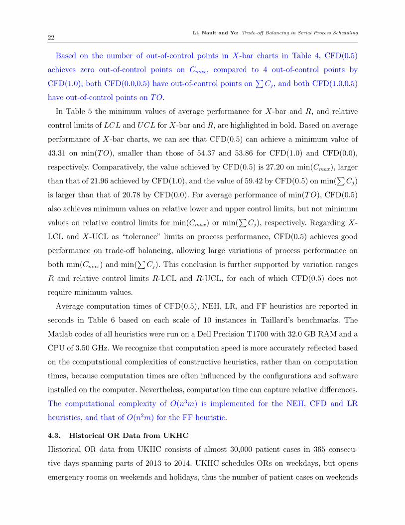
Based on the number of out-of-control points in X-bar charts in Table 4, CFD(0.5)
achieves zero out-of-control points on Cmax, compared to 4 out-of-control points by
CFD(1.0); both CFD(0.0,0.5) have out-of-control points on∑Cj, and both CFD(1.0,0.5)
have out-of-control points on TO.
In Table 5 the minimum values of average performance for X-bar and R, and relative
control limits of LCL and UCL for X-bar and R, are highlighted in bold. Based on average
performance of X-bar charts, we can see that CFD(0.5) can achieve a minimum value of
43.31 on min(TO), smaller than those of 54.37 and 53.86 for CFD(1.0) and CFD(0.0),
respectively. Comparatively, the value achieved by CFD(0.5) is 27.20 on min(Cmax), larger
than that of 21.96 achieved by CFD(1.0), and the value of 59.42 by CFD(0.5) on min(∑Cj)
is larger than that of 20.78 by CFD(0.0). For average performance of min(TO), CFD(0.5)
also achieves minimum values on relative lower and upper control limits, but not minimum
values on relative control limits for min(Cmax) or min(∑Cj), respectively. Regarding X-
LCL and X-UCL as “tolerance” limits on process performance, CFD(0.5) achieves good
performance on trade-off balancing, allowing large variations of process performance on
both min(Cmax) and min(∑Cj). This conclusion is further supported by variation ranges
R and relative control limits R-LCL and R-UCL, for each of which CFD(0.5) does not
require minimum values.
Average computation times of CFD(0.5), NEH, LR, and FF heuristics are reported in
seconds in Table 6 based on each scale of 10 instances in Taillard’s benchmarks. The
Matlab codes of all heuristics were run on a Dell Precision T1700 with 32.0 GB RAM and a
CPU of 3.50 GHz. We recognize that computation speed is more accurately reflected based
on the computational complexities of constructive heuristics, rather than on computation
times, because computation times are often influenced by the configurations and software
installed on the computer. Nevertheless, computation time can capture relative differences.
The computational complexity of O(n3m) is implemented for the NEH, CFD and LR
heuristics, and that of O(n2m) for the FF heuristic.
4.3. Historical OR Data from UKHC
Historical OR data from UKHC consists of almost 30,000 patient cases in 365 consecu-
tive days spanning parts of 2013 to 2014. UKHC schedules ORs on weekdays, but opens
emergency rooms on weekends and holidays, thus the number of patient cases on weekends
Li, Nault and Ye: Trade-off Balancing in Serial Process Scheduling23
Table 6 Average Computation Times on Taillard’s Benchmarks (Sec.)
Computation Time
n by m CFD(0.5) NEH LR(1) FF 20 by 5 0.02 0.00 0.03 0.00
20 by 10 0.02 0.00 0.04 0.00 20 by 20 0.01 0.00 0.03 0.00 50 by 5 0.05 0.00 0.17 0.00
50 by 10 0.06 0.00 0.16 0.00 50 by 20 0.05 0.01 0.16 0.00 100 by 5 0.17 0.01 0.58 0.00
100 by 10 0.21 0.04 0.67 0.00 100 by 20 0.25 0.07 0.72 0.01 200 by 10 1.11 0.29 3.16 0.06 200 by 20 1.45 0.59 4.03 0.10 500 by 20 18.91 9.79 53.18 0.60
Avg 1.86 0.90 5.24 0.07
and holidays is much less than that on weekdays. Excluding data points on weekends and
holidays, we have more than 28,000 patient cases in 260 days used in our case study.
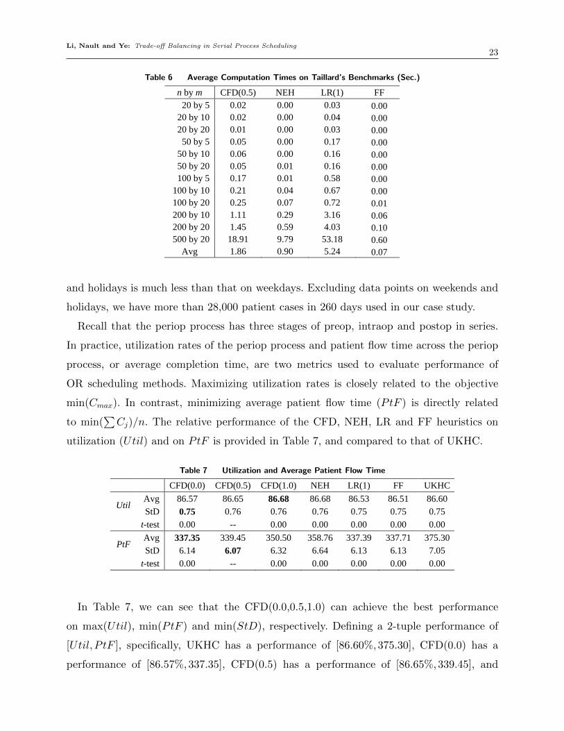
Recall that the periop process has three stages of preop, intraop and postop in series.
In practice, utilization rates of the periop process and patient flow time across the periop
process, or average completion time, are two metrics used to evaluate performance of
OR scheduling methods. Maximizing utilization rates is closely related to the objective
min(Cmax). In contrast, minimizing average patient flow time (PtF ) is directly related
to min(∑Cj)/n. The relative performance of the CFD, NEH, LR and FF heuristics on
utilization (Util) and on PtF is provided in Table 7, and compared to that of UKHC.
Table 7 Utilization and Average Patient Flow TimeTable 5 Utilization and Average Patient Flow
CFD(0.0) CFD(0.5) CFD(1.0) NEH LR(1) FF UKHC
Util Avg 86.57 86.65 86.68 86.68 86.53 86.51 86.60
StD 0.75 0.76 0.76 0.76 0.75 0.75 0.75
t-test 0.00 -- 0.00 0.00 0.00 0.00 0.00
PtF Avg 337.35 339.45 350.50 358.76 337.39 337.71 375.30
StD 6.14 6.07 6.32 6.64 6.13 6.13 7.05
t-test 0.00 -- 0.00 0.00 0.00 0.00 0.00
In Table 7, we can see that the CFD(0.0,0.5,1.0) can achieve the best performance
on max(Util), min(PtF ) and min(StD), respectively. Defining a 2-tuple performance of
[Util,P tF ], specifically, UKHC has a performance of [86.60%,375.30], CFD(0.0) has a
performance of [86.57%,337.35], CFD(0.5) has a performance of [86.65%,339.45], and
Li, Nault and Ye: Trade-off Balancing in Serial Process Scheduling24
CFD(1.0) has a performance of [86.68%,350.50]. Given the performance of [86.68%,358.76],
[86.53%,337.39] and [86.51%,337.71] for the NEH, LR and FF heuristics, respectively, we
can see that CFD(1.0) dominates NEH, and CFD(0.0) dominates LR and FF, for OR
scheduling based on Util and on PtF across the periop process. All scheduling methods
are significantly different from each other based on p-values of t-tests against CFD(0.5).
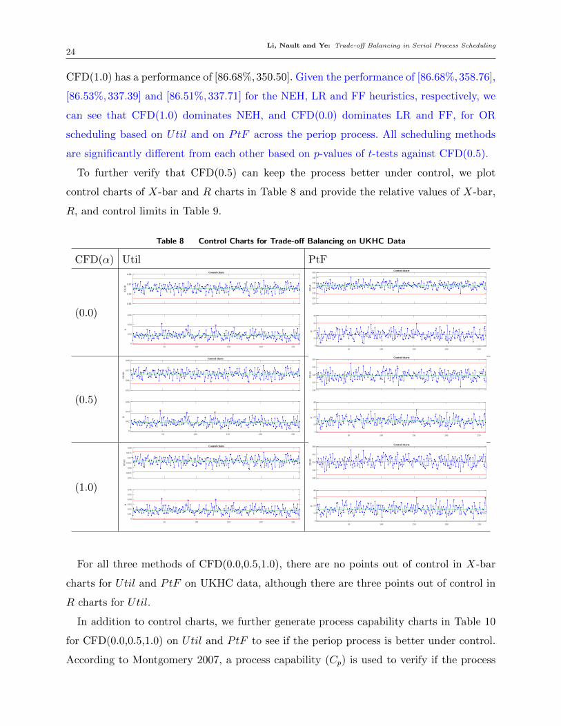
To further verify that CFD(0.5) can keep the process better under control, we plot
control charts of X-bar and R charts in Table 8 and provide the relative values of X-bar,
R, and control limits in Table 9.
Table 8 Control Charts for Trade-off Balancing on UKHC Data
CFD(α) Util PtF
(0.0)0.85
0.86
0.87
0.88
XB
AR
Control charts
50 100 150 200 2500
0.02
0.04
0.06
R
320
325
330
335
340
345
350
XB
AR
Control charts
50 100 150 200 250
0
10
20
30
40
R
(0.5)0.85
0.86
0.87
0.88
XB
AR
Control charts
50 100 150 200 2500
0.02
0.04
0.06
R
330
335
340
345
350
XB
AR
Control charts
50 100 150 200 250
0
10
20
30
40
R
(1.0)0.85
0.855
0.86
0.865
0.87
0.875
0.88
XB
AR
Control charts
50 100 150 200 2500
0.01
0.02
0.03
0.04
0.05
0.06
R
340
345
350
355
360
XB
AR
Control charts
50 100 150 200 250
0
10
20
30
40
R
For all three methods of CFD(0.0,0.5,1.0), there are no points out of control in X-bar
charts for Util and PtF on UKHC data, although there are three points out of control in
R charts for Util.
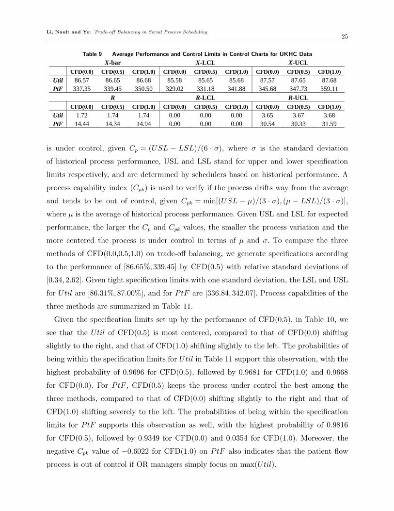
In addition to control charts, we further generate process capability charts in Table 10
for CFD(0.0,0.5,1.0) on Util and PtF to see if the periop process is better under control.
According to Montgomery 2007, a process capability (Cp) is used to verify if the process
Li, Nault and Ye: Trade-off Balancing in Serial Process Scheduling25
Table 9 Average Performance and Control Limits in Control Charts for UKHC DataTable 7 Average Performance and Control Limits in Control Charts for UKHC Data
X-bar X-LCL X-UCL
CFD(0.0) CFD(0.5) CFD(1.0) CFD(0.0) CFD(0.5) CFD(1.0) CFD(0.0) CFD(0.5) CFD(1.0)
Util 86.57 86.65 86.68 85.58 85.65 85.68 87.57 87.65 87.68 PtF 337.35 339.45 350.50 329.02 331.18 341.88 345.68 347.73 359.11
R R-LCL R-UCL
CFD(0.0) CFD(0.5) CFD(1.0) CFD(0.0) CFD(0.5) CFD(1.0) CFD(0.0) CFD(0.5) CFD(1.0)
Util 1.72 1.74 1.74 0.00 0.00 0.00 3.65 3.67 3.68 PtF 14.44 14.34 14.94 0.00 0.00 0.00 30.54 30.33 31.59
is under control, given Cp = (USL − LSL)/(6 · σ), where σ is the standard deviation
of historical process performance, USL and LSL stand for upper and lower specification
limits respectively, and are determined by schedulers based on historical performance. A
process capability index (Cpk) is used to verify if the process drifts way from the average
and tends to be out of control, given Cpk = min[(USL − µ)/(3 · σ), (µ − LSL)/(3 · σ)],
where µ is the average of historical process performance. Given USL and LSL for expected
performance, the larger the Cp and Cpk values, the smaller the process variation and the
more centered the process is under control in terms of µ and σ. To compare the three
methods of CFD(0.0,0.5,1.0) on trade-off balancing, we generate specifications according
to the performance of [86.65%,339.45] by CFD(0.5) with relative standard deviations of
[0.34,2.62]. Given tight specification limits with one standard deviation, the LSL and USL
for Util are [86.31%,87.00%], and for PtF are [336.84,342.07]. Process capabilities of the
three methods are summarized in Table 11.
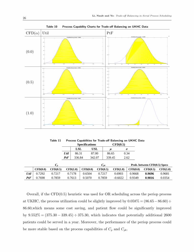
Given the specification limits set up by the performance of CFD(0.5), in Table 10, we
see that the Util of CFD(0.5) is most centered, compared to that of CFD(0.0) shifting
slightly to the right, and that of CFD(1.0) shifting slightly to the left. The probabilities of
being within the specification limits for Util in Table 11 support this observation, with the
highest probability of 0.9696 for CFD(0.5), followed by 0.9681 for CFD(1.0) and 0.9668
for CFD(0.0). For PtF , CFD(0.5) keeps the process under control the best among the
three methods, compared to that of CFD(0.0) shifting slightly to the right and that of
CFD(1.0) shifting severely to the left. The probabilities of being within the specification
limits for PtF supports this observation as well, with the highest probability of 0.9816
for CFD(0.5), followed by 0.9349 for CFD(0.0) and 0.0354 for CFD(1.0). Moreover, the
negative Cpk value of −0.6022 for CFD(1.0) on PtF also indicates that the patient flow
process is out of control if OR managers simply focus on max(Util).
Li, Nault and Ye: Trade-off Balancing in Serial Process Scheduling26
Table 10 Process Capability Charts for Trade-off Balancing on UKHC Data
CFD(α) Util PtF
(0.0)
0.855 0.86 0.865 0.87 0.875 0.88 0.8850
20
40
60
80
100
120Probability Between Limits = 0.96681
328 330 332 334 336 338 340 342 344 3460
0.05
0.1
0.15Probability Between Limits = 0.93489
(0.5)
0.855 0.86 0.865 0.87 0.875 0.88 0.8850
20
40
60
80
100
120Probability Between Limits = 0.96962
330 332 334 336 338 340 342 344 346 3480
0.02
0.04
0.06
0.08
0.1
0.12
0.14
0.16Probability Between Limits = 0.98161
(1.0)
0.855 0.86 0.865 0.87 0.875 0.88 0.8850
20
40
60
80
100
120Probability Between Limits = 0.96813
330 335 340 345 350 355 3600
0.05
0.1
0.15Probability Between Limits = 0.035415
Table 11 Process Capabilities for Trade-off Balancing on UKHC DataTable 9 Process Capabilities of Trade-off Balancing for UKHC Data Specifications CFD(0.5)
LSL USL μ σ
Util 86.31 87.00 86.65 0.34 PtF 336.84 342.07 339.45 2.62
Cp Cpk Prob. between CFD(0.5) Specs CFD(0.0) CFD(0.5) CFD(1.0) CFD(0.0) CFD(0.5) CFD(1.0) CFD(0.0) CFD(0.5) CFD(1.0)
Util 0.7292 0.7217 0.7178 0.6504 0.7217 0.6903 0.9668 0.9696 0.9681 PtF 0.7698 0.7859 0.7613 0.5070 0.7859 -0.6022 0.9349 0.9816 0.0354
Overall, if the CFD(0.5) heuristic was used for OR scheduling across the periop process
at UKHC, the process utilization could be slightly improved by 0.058% = (86.65−86.60)÷
86.60,which means some cost saving, and patient flow could be significantly improved
by 9.552% = (375.30− 339.45)÷ 375.30, which indicates that potentially additional 2600
patients could be served in a year. Moreover, the performance of the periop process could
be more stable based on the process capabilities of Cp and Cpk.
Li, Nault and Ye: Trade-off Balancing in Serial Process Scheduling27
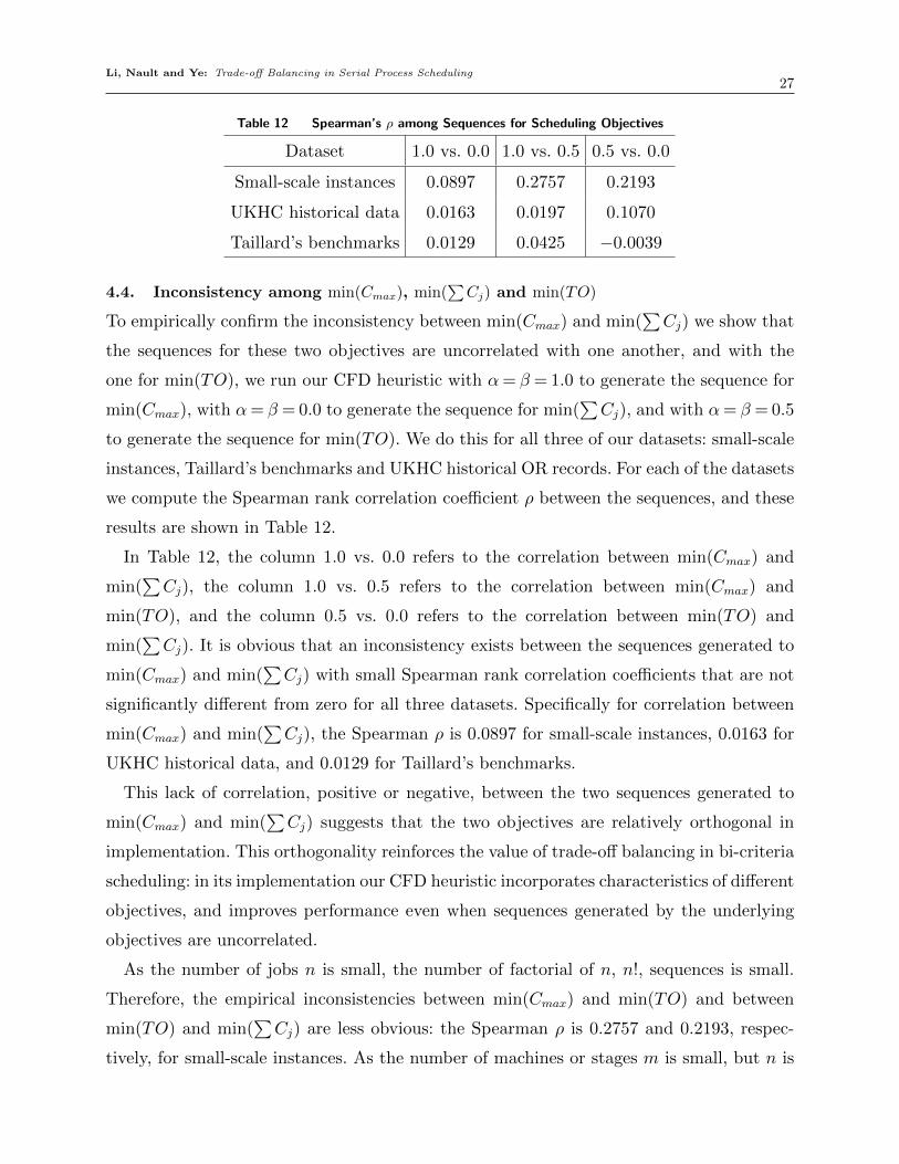
Table 12 Spearman’s ρ among Sequences for Scheduling Objectives
Dataset 1.0 vs. 0.0 1.0 vs. 0.5 0.5 vs. 0.0
Small-scale instances 0.0897 0.2757 0.2193
UKHC historical data 0.0163 0.0197 0.1070
Taillard’s benchmarks 0.0129 0.0425 −0.0039
4.4. Inconsistency among min(Cmax), min(∑Cj) and min(TO)
To empirically confirm the inconsistency between min(Cmax) and min(∑Cj) we show that
the sequences for these two objectives are uncorrelated with one another, and with the
one for min(TO), we run our CFD heuristic with α= β = 1.0 to generate the sequence for
min(Cmax), with α= β = 0.0 to generate the sequence for min(∑Cj), and with α= β = 0.5
to generate the sequence for min(TO). We do this for all three of our datasets: small-scale
instances, Taillard’s benchmarks and UKHC historical OR records. For each of the datasets
we compute the Spearman rank correlation coefficient ρ between the sequences, and these
results are shown in Table 12.
In Table 12, the column 1.0 vs. 0.0 refers to the correlation between min(Cmax) and
min(∑Cj), the column 1.0 vs. 0.5 refers to the correlation between min(Cmax) and
min(TO), and the column 0.5 vs. 0.0 refers to the correlation between min(TO) and
min(∑Cj). It is obvious that an inconsistency exists between the sequences generated to
min(Cmax) and min(∑Cj) with small Spearman rank correlation coefficients that are not
significantly different from zero for all three datasets. Specifically for correlation between
min(Cmax) and min(∑Cj), the Spearman ρ is 0.0897 for small-scale instances, 0.0163 for
UKHC historical data, and 0.0129 for Taillard’s benchmarks.
This lack of correlation, positive or negative, between the two sequences generated to
min(Cmax) and min(∑Cj) suggests that the two objectives are relatively orthogonal in
implementation. This orthogonality reinforces the value of trade-off balancing in bi-criteria
scheduling: in its implementation our CFD heuristic incorporates characteristics of different
objectives, and improves performance even when sequences generated by the underlying
objectives are uncorrelated.
As the number of jobs n is small, the number of factorial of n, n!, sequences is small.
Therefore, the empirical inconsistencies between min(Cmax) and min(TO) and between
min(TO) and min(∑Cj) are less obvious: the Spearman ρ is 0.2757 and 0.2193, respec-
tively, for small-scale instances. As the number of machines or stages m is small, but n is
Li, Nault and Ye: Trade-off Balancing in Serial Process Scheduling28
large, the empirical inconsistency between min(Cmax) and min(TO) is obvious for UKHC
historical data with a Spearman ρ of 0.0197, but that between min(TO) and min(∑Cj) is
less obvious with a Spearman ρ of 0.1070. However, as both n and m are large, the empirical
inconsistencies between min(Cmax) and min(TO) and between min(TO) and min(∑Cj) are
obvious for Taillard’s benchmarks with the Spearman ρ of 0.0425 and −0.0039, respectively.
Such lack of pairwise correlation between sequences generated among three objectives indi-
cate that process design should take the number of jobs and the number of operations into
consideration. For example, if the periop process at UKHC was separated into more than
three stages, or a stage was finely tuned into several operations, the inconsistency between
min(TO) and min(∑Cj) might be obvious as well.
5. Conclusion and Future Work
Given the property of NP -completeness for each of min(Cmax) and min(∑Cj) scheduling
problems, we model the trade-offs by two coupled deviations, providing an innovative and
systematic approach for modeling scheduling problems for serial processes. Based on this
new approach to model scheduling problems, we provide an effective interpretation con-
cerning deviations at the operation level and at the process level, where current deviations
should be taken into consideration for min(Cmax), but both current and future devia-
tions should be considered for min(∑Cj). This is because maximum completion time is
purely determined by the sum of idle times for deterministic problems, and future idle
times in U are influenced by current completion times of jobs in S, but not the other way
around. However, total completion time is determined by the sum of weighted idle times
and weighted processing times, which means jobs in both S and U interact with each other
on min(∑Cj).
Our systematic approach of analyzing two coupled deviations in our heuristic develop-
ment helps us address the concern about dominance evaluation as in Pareto efficiency,
whereby we should put equal preferences for balancing trade-offs between min(Cmax) and
min(∑Cj). This answers the first question that near-optimal solutions to min(Cmax) or
to min(∑Cj) cannot balance the trade-offs given the inconsistency between simple objec-
tives. Modelling coupled deviations from upper and lower bounds of completion times by
α, and balancing trade-offs between output variables by β, means our CFD heuristic is
sufficiently flexible to address management concerns at both operation and process levels.
Li, Nault and Ye: Trade-off Balancing in Serial Process Scheduling29
Through case studies on 5400 small-scale instances, our CFD heuristic outperforms the
NEH, LR, and FF heuristics on trade-off balancing, and on min(Cmax) and min(∑Cj),
respectively. Through case studies on 120 instances in Taillard’s benchmarks, the FF heuris-
tic marginally outperforms our CFD heuristic only on min(∑Cj), but not on our other
performance metrics, and our CFD heuristic outperforms the NEH and LR heuristic on
all of our performance metrics.
Our approach to model trade-offs between min(Cmax) and min(∑Cj) and our CFD
heuristic provide a solid starting point for balancing trade-offs in serial processes, especially
for OR scheduling across the periop process. Based on case studies of Taillard’s benchmarks
and historical OR data at UKHC, trade-off balancing can keep the process better under
control, where the average trade-off values vary in a tight range, but with wider variation
ranges allowable for Cmax and for∑Cj, respectively, the utilization and the patient flow
time are improved across the periop process, and the periop process is more under control
using our CFD heuristic for scheduling.
Dynamically updating the lower and upper bounds of completion times at the process
level is part of our future work in heuristic development for better trade-off balancing. This
is because our analysis of deviations is more effective for small-scale instances, on which
our CFD heuristic clearly dominates the NEH, LR and FF heuristics on min(Cmax) and
min(∑Cj), respectively, but less effective on min(
∑Cj) for Taillard’s benchmarks.
Acknowledgments
This project was supported by grant number R03HS024633 from the Agency for Healthcare Research and
Quality. The content is solely the responsibility of the authors and does not necessarily represent the official
views of the Agency for Healthcare Research and Quality. We appreciate support from UK HealthCare, the
Department of Mechanical Engineering at University of Kentucky, the Natural Sciences and Engineering
Research Council of Canada, and the Haskayne School of Business at University of Calgary. We thank
Jeanette Burman for editing assistance.
References
AHRQ (2013) National healthcare quality report. Available at http://www.ahrq.gov/sites/default/
files/publications/files/2013nhqr.pdf.
Ciavotta M, Minella G, Ruiz R (2013) Multi-objective sequence dependent setup times permutation flowshop:
A new algorithm and a comprehensive study. European Journal of Operational Research 227(2):3001–
313.
Li, Nault and Ye: Trade-off Balancing in Serial Process Scheduling30
Czyzak P, Jaszkiewics A (1998) Pareto-simulated annealinga metaheuristic technique for multi-objective
combinatorial optimization. Journal of Multi-criteria Decision Analysis 7(1):34–47.
Ding JY, Song S, Wu C (2016) Carbon-efficient scheduling of flow shops by multi-objective optimization.
European Journal of Operational Research 248(3):758–771.
Fang K, Uhan N, Zhao F, Sutherland JW (2011) A new approach to scheduling in manufacturing for power
consumption and carbon footprint reduction. Journal of Manufacturing Systems 30(4):234–240.
Fernandez-Viagas V, Framinan JM (2015) A new set of high-performing heuristics to minimise flowtime in
permutation flowshops. Computers & Operations Research 53:68–80.
Figueira JR, Liefooghe A, Talbi EG, Wierzbicki AP (2010) A parallel multiple reference point approach for
multi-objective optimization. European Journal of Operational Research 205(2):390–400.
Framinan JM (2009) A fitness-based weighting mechanism for multicriteria flowshop scheduling using genetic
algorithms. International Journal of Advanced Manufacturing Technology 43(9–10):939–948.
Framinan JM, Gupta JN, Leisten R (2004) A review and classification of heuristics for permutation flow-shop
scheduling with makespan objective. Journal of the Operational Research Society 55(12):1243–1255.
Framinan JM, Leisten R, Ruiz-Usano R (2002) Efficient heuristics for flowshop sequencing with the objectives
of makespan and flowtime minimisation. European Journal of Operational Research 141(3):559–569.
Gahm C, Denz F, Dirr M, Tuma A (2016) Energy-efficient scheduling in manufacturing companies: a review
and research framework. European Journal of Operational Research 248(3):744–757.
Garey MR, Johnson DS, Sethi R (1976) The complexity of flowshop and jobshop scheduling. Mathematics
of Operations Research 1(2):117–129.
GeneralElectric (2014) Audited financial statements and notes. Available at https://www.ge.com/ar2014/
assets/pdf/GE_AR14_AuditedFinancialStatement.pdf.
Gul S, Denton BT, Fowler JW, Huschka T (2011) Bi-criteria scheduling of surgical services for an outpatient
procedure center. Production and Operations Management 20(3):406–417.
Gupta D, Denton B (2008) Appointment scheduling in health care: Challenges and opportunities. IIE Trans-
actions 40(9):800–819.
Gupta JN, Stafford EF (2006) Flowshop scheduling research after five decades. European Journal of Opera-
tional Research 169(3):699–711.
Harris FW (1990) How many parts to make at once. Operations Research 38(6):947–950.
Ho JC (1995) Flowshop sequencing with mean flowtime objective. European Journal of Operational Research
81(3):571–578.
Hoogeveen J, Kawaguchi T (1999) Minimizing total completion time in a two-machine flowshop: analysis of
special cases. Mathematics of Operations Research 24(4):887–910.
Li, Nault and Ye: Trade-off Balancing in Serial Process Scheduling31
Hopp WJ, Spearman ML (2000) Factory physics (Waveland Press).
Ishibuchi H, Yoshida T, Murata T (2003) Balance between genetic search and local search in memetic
algorithms for multiobjective permutation flowshop scheduling. IEEE Transactions on Evolutionary
Computation 7(2):204–223.
Johnson SM (1954) Optimal two-and three-stage production schedules with setup times included. Naval
Research Logistics–Quaterly 1(1):61–68.
Kalczynski PJ, Kamburowski J (2007) On the neh heuristic for minimizing the makespan in permutation
flow shops. Omega–The International Journal of Management Science 35(1):53–60.
Kim YD (1995) Minimizing total tardiness in permutation flowshops. European Journal of Operational
Research 85(3):541–555.
Li W, Luo X, Xue D, Tu Y (2011a) A heuristic for adaptive production scheduling and control in flow shop
production. International Journal of Production Research 49(11):3151–3170.
Li W, Mitchell VL, Nault BR (2014) Inconsistent objectives in operating room scheduling. IIE Annual
Conference. Proceedings, 727–736 (Institute of Industrial and Systems Engineers (IISE)).
Li W, Nault BR, Xue D, Tu Y (2011b) An efficient heuristic for adaptive production scheduling and control
in one-of-a-kind production. Computers & Operations Research 38(1):267–276.
Liu J, Reeves CR (2001) Constructive and composite heuristic solutions to the p||∑ci scheduling problem.
European Journal of Operational Research 132(2):439–452.
Magerlein JM, Martin JB (1978) Surgical demand scheduling: a review. Health Services Research 13(4):418.
Malakooti B (2013) Operations and production systems with multiple objectives (John Wiley & Sons).
Montgomery DC (2007) Introduction to Statistical Quality Control (John Wiley & Sons).
Nawaz M, Enscore EE, Ham I (1983) A heuristic algorithm for the m-machine, n-job flow-shop sequencing
problem. Omega–The International Journal of Management Science 11(1):91–95.
Orlicky J (1975) Material requirements planning (McGraw-Hill Education: New York).
Pinedo ML (2008) Scheduling: Theory, Algorithms, and Systems (Springer Publishing Company, Incorpo-
rated).
Ruiz R, Maroto C (2005) A comprehensive review and evaluation of permutation flowshop heuristics. Euro-
pean Journal of Operational Research 165(2):479–494.
Slowinski R (1981) Multiobjective network scheduling with efficient use of renewable and nonrenewable
resources. European Journal of Operational Research 7(3):265–273.
Slowinski R, Weglarz J (1989) Advances in Project Scheduling (Elsevier).
Stevenson WJ (2009) Operations Management (McGraw-Hill Education: New York).

Li, Nault and Ye: Trade-off Balancing in Serial Process Scheduling32
Taillard E (1990) Some efficient heuristic methods for the flow shop sequencing problem. European Journal
of Operational Research 47(1):65–74.
Taillard E (1993) Benchmarks for basic scheduling problems. European Journal of Operational Research
64(2):278–285.
T’kindt V, Billaut JC (2002) Multicriteria Scheduling: Theory, Models, and Algorithms (Springer).
Ye H, Li W, Abedini A, Nault B (2017) An effective and efficient heuristic for no-wait flow shop production
to minimize total completion time. Computers & Industrial Engineering 108:57–69.
Zhang H, Zhao F, Fang K, Sutherland JW (2014) Energy-conscious flow shop scheduling under time-of-use
electricity tariffs. CIRP Annals-Manufacturing Technology 63(1):37–40.