Noname manuscript No.(will be inserted by the editor)

Performance Analysis and Functional Verification of theStop-and-Wait Protocol in HOL

Osman Hasan · Sofiene Tahar

Received: date / Accepted: date

Abstract Real-time systems usually involve a subtle interaction of a number of dis-

tributed components and have a high degree of parallelism, which makes their perfor-

mance analysis quite complex. Thus, traditional techniques, such as simulation, or the

state-based formal methods usually fail to produce reasonable results. In this paper,

we propose to use higher-order-logic theorem proving for the performance analysis of

real-time systems. The idea is to formalize the real-time system as a logical conjunc-

tion of higher-order-logic predicates, whereas each one of these predicates define an

autonomous component or process of the given real-time system. The random or un-

predictable behavior found in these components is modeled as random variables. This

formal specification can then be used in a higher-order-logic theorem prover (HOL) to

reason about both functional and performance related properties of the given real-time

system. In order to illustrate the practical effectiveness of our approach, we present

the analysis of the Stop-and-Wait protocol, which is a classical example of real-time

systems. The functional correctness of the protocol is verified by proving that the pro-

tocol ensures reliable data transfers. Whereas, the average message delay relation is

verified in HOL for the sake of performance analysis. The paper includes the protocol’s

formalization details along with the HOL proof sketches for the major theorems.

Keywords Communication Protocols · Higher-order-logic · HOL Theorem Prover ·Probability Theory · Real-Time Systems

1 Introduction

Real-time systems can be characterized as systems for which the correctness of an op-

eration is dependant not only on its logical correctness but also on the time taken.

Osman HasanDepartment of Electrical and Computer Engineering, Concordia University,1455 de Maisonneuve W., Montreal, Quebec, H3G 1M8, CanadaE-mail: o hasan@ece.concordia.ca

Sofiene TaharDepartment of Electrical and Computer Engineering, Concordia University,1455 de Maisonneuve W., Montreal, Quebec, H3G 1M8, CanadaE-mail: tahar@ece.concordia.ca

2

Table 1 CDF of Message Delay

t(sec) Protocol 1 Protocol 2

20 0.92 040 0.94 060 0.96 080 0.98 0100 1 1

Some commonly used real-time system applications include embedded systems, digi-

tal circuits with uncertain delays and communication protocols. Due to the increased

usage of real-time systems in safety critical and extremely sensitive applications such

as medicine, military and space travel, their correctness and performance has become

imperative. The functional verification and performance evaluation tasks in this do-

main are quite challenging as the present age real-time systems usually involve a subtle

interaction of a number of distributed components and have a high degree of paral-

lelism. The level of sophistication found in current real-time systems demands formal

specification of requirements and thus traditional techniques, like simulation, fail to

provide the necessary level of assuredness about what is being built is actually what

was intended. On the other hand, formal methods offer a promising solution.

A number of elegant approaches for the formal functional verification of real-time

systems can be found in the open literature using state-based or theorem proving

techniques (e.g. [1,7,2,3]). However, most of these existing formal verification tools are

only capable of specifying and verifying hard deadlines, i.e., properties where a late

response is considered to be incorrect. For example, while proving the message delivery

characteristic of a communication protocol, we can only check if the message is delivered

for sure within a specific duration in time, say 100 seconds, for all possible scenarios.

Even though this information is quite useful for establishing functional correctness, it

usually proves to be quite insufficient for performance analysis. Consider the example of

two communication protocols for which the Cumulative Distribution Function (CDF)

of the message delay, i.e., the probability that the message delay is less than or equal

to time t, is given in Table 1. Both protocols satisfy the hard deadline of a message

being delivered within 100 seconds as the probability of the message delay being less

than or equal to 100 seconds is 1. Now, it can also be observed that they do not satisfy

the hard deadline of the message being delivered within 80 seconds as for both of them

there exist some cases for which the message is not delivered. So from the perspective of

these hard deadline verification results, both protocols seem to behave quite similarly

and the huge difference in the performance of the two protocols remains hidden.

The above example clearly demonstrates the significance of verifying soft deadlines,

i.e., properties that provide the quality of service in terms of probabilistic quantities or

averages, for performance analysis of real-time systems. Recently, several state-based

formal approaches have been proposed for the verification of soft deadlines for real-

time systems (e.g. [27,6,26]). However, all these approaches share the same inherent

limitation that is the reduced expressive power of their automata based or Petri net

based specification formalism. On top of that, either there is no mechanism to verify

the expectation or average value in these techniques or even if it does exist then the

underlying infrastructure cannot be regarded as completely formal. Whereas, expecta-

tion is considered to be one of the most widely used characteristics for the performance

3

analysis of real-time systems, since it tends to summarize the probability distribution

of the random variable in a single number. For example, in the PRISM model checker

[25], probabilistic models can be augmented with cost or rewards, i.e., real values as-

sociated with certain states or transitions of the model, which allows us to analyze the

average values related to these rewards. Duflot et al. [11] used this aspect of PRISM

to conduct the performance analysis of a CSMA/CD protocol, which is a real-time

communication protocol. It is important to note that the meaning ascribed to these

properties is, of course, dependent on the definitions of the rewards themselves and

thus the solutions obtained using this kind of approaches are approximate as has been

clearly stated in [11].

Due to the immaturity of formal methods in verifying soft deadlines and using them

for performance evaluation of real-time systems, the current state-of-the-art is based on

constructing abstract models that are analyzed by simulation or by applying stochastic

process theory using paper-and-pencil proof methods. Besides the inaccuracy of results

by simulation based methods and the drawbacks associated with paper-and-pencil proof

methods, a major limitation of this approach is that the model used for performance

analysis is usually quite far in abstraction level from the one used for formal functional

verification. This fact makes the equivalence verification between these two models

very difficult, if not impossible, and thus leaves a major gap in the completeness of the

functional verification and performance analysis tasks. These kind of limitations may

lead to inaccurate performance analysis, which in turn can have disastrous consequences

if the given real-time system is to be used in a safety or financial critical domain. One

of the well-known incidents in this regard include the loss, in December 1999, of the

Mars Polar Lander [29]; a $165 million NASA spacecraft launched to survey Martian

conditions. The Mars Polar Lander is believed to be lost mainly because of its engine

shutdown while it was still 40 meters above the Mars surface. The engine shutdown

happened due to the vibrations caused by the deployment of the lander’s legs, i.e.,

a probabilistic behavior, that gave false indication that spacecraft had landed. Some

other such incidents related to inaccurate or inadequate performance analysis of real-

time systems include the loss of $125 million Mars Climate Orbiter [28] in 1998 and

the performance degradation of the Microsofts IIS indexing service DLL due to the

buffer overflow problem caused by the “Code Red” worm in 2001 [9], which resulted in

a loss of over $2 billion to the company. A more recent incident is the faulty operation

of the fly-by-wire primary flight control real-time software of a Boeing 777, operated

by the Malaysia Airlines, in August 2005 [5], which could have resulted in the loss of

177 passenger lives if the pilot had not manually taken over the autopilot program in

time.

To overcome the above mentioned limitations of existing performance analysis tech-

niques, we propose to conduct the performance evaluation of real-time systems within

the sound core of a higher-order-logic theorem prover [14]. The main motivation behind

this choice is to leverage upon the high expressiveness of higher-order-logic to formally

specify and reason about the temporal properties and random behaviors of the present

age complex real-time systems. The proposed approach is primarily based upon the

previous work reported for the functional verification of hard real-time systems [7], the

formalization of random variables [23] and the verification of expectation properties

for discrete random variables [19]. The idea is to formally specify the given real-time

system as a logical conjunction of higher-order-logic predicates [7], whereas each one

of these predicates defines an autonomous component or process of the given real-

time system, while representing the unpredictable or random elements in the system

4

as formalized random variables [23]. The functional correctness and the expectation

properties for various parameters for this formal model can then be verified using an

interactive theorem prover with the help of the useful theorems already proved in [7,

23,19]. Since the analyses is conducted within the core of a mechanical theorem prover,

there would be no question about the soundness or the precision of the results. Also,

there is no equivalence verification required between the models used for functional

verification and performance evaluation as the same formal model is used for both of

these analysis in this approach. On the other hand, the downside of the above approach

is the associated significant user interaction. It is important to note here that the pro-

posed approach should not be viewed as an alternative to methods such as simulation

and model-checking for the performance analysis of real-time systems but rather as a

complementary technique.

In order to illustrate the practical effectiveness of our approach, this paper presents

the functional verification and performance analysis of a variant of the Stop-and-Wait

protocol [13], which is a classical example of a real-time system. The Stop-and-Wait

protocol utilizes the principles of error detection and retransmission and is a funda-

mental mechanism for reliable communication between computers. Indeed, it is one

of the most important part of the Internet’s Transmission Control Protocol (TCP).

The main motivation behind selecting the Stop-and-Wait protocol as a case study for

our approach is its widespread popularity in the literature regarding real-time system

analysis methodologies. The Stop-and-Wait protocol and some of its closely related

variants have been checked formally for functional verification using theorem proving

[7], state-based formal approaches [35,4,12] and a combination of both techniques [22]

and their performance has been analyzed using a number of innovative state-based for-

mal or semi-formal techniques (e.g. [30,33,37,15]). But like other real-time systems, to

the best of our knowledge, there is no mechanized approach reported in the literature

that utilizes a single model of the Stop-and-Wait protocol and could verify its func-

tional correctness and precisely analyze its performance. This paper tends to fill this

gap as we present the functional verification and the performance analysis, based on

the precise average delay for a single message transmission, for the Stop-and-Wait pro-

tocol using the HOL theorem prover [17]. We have chosen HOL in order to build upon

the existing formalization presented in [7,23,19]. The proposed approach is not specific

to the HOL theorem prover though and can be adapted to any other higher-order-logic

theorem prover, such as Isabelle [31] and PVS [32], as well.

The variant of the Stop-and-Wait protocol that is analyzed in this paper utilizes

two distinct sequence numbers (0 and 1) and is usually termed as the Alternating

Bit Protocol (ABP). The analysis is done assuming an ideal (noiseless) channel for

ACK messages, a fixed value of channel propagation delay for both data and ACK

messages and a fixed value of 1 unit time for the processing delay at both sender and

receiver stations. The main intent behind using these assumptions is to reduce the

proof clutter and thus to simplify the understandability of the proofs presented in this

paper. If required, these assumptions can be removed and a more generalized version

of the Stop-and-Wait protocol can also be verified using the methodology presented in

this paper. For example, the channel for the ACK messages can be made noisy using

the approach for handling the noisy data message channel illustrated in this paper.

Similarly, the processing delay can be made a variable quantity by using a similar

approach that we use to handle the variable time-out and data transmission delays.

The rest of the paper is organized as follows. Section 2 provides an overview of mod-

eling random variables and verifying their expectation properties in HOL. In Section 3,

5

we present an informal description of the Stop-and-Wait protocol along with its average

delay characteristic. Next, in Section 4, we present a higher-order-logic specification of

the Stop-and-Wait protocol. We verify the functional correctness of this specification

using the HOL theorem prover in Section 5. Then, in Section 6, we conduct the perfor-

mance analysis of the Stop-and-Wait protocol based on its formal specification in HOL.

We mainly verify the message delay characteristic of the Stop-and-Wait protocol, which

is the most widely used performance measuring parameter for communication proto-

cols, first under noise-free conditions and then with the consideration of the channel

noise. Finally, Section 7 concludes the paper.

2 Random Variables and their Expectation in HOL

This section first summarizes a methodology for the formalization of probabilistic al-

gorithms [23], which in turn can be used to model random variables as well. Then we

present a higher-order-logic formalization of the expectation theory [19], which allows

us to verify mean or average values associated with discrete random variables in HOL.

The intent is to introduce the main ideas along with some notation that is going to be

used in the next sections.

2.1 Formalization of Random Variables in HOL

Random variables are the core component of conducting probabilistic performance

analysis of real-time systems. They can be formalized in higher-order logic as deter-

ministic functions with access to an infinite Boolean sequence B∞; a source of infinite

random bits [23]. These deterministic functions make random choices based on the re-

sult of popping the top most bit in the infinite Boolean sequence and may pop as many

random bits as they need for their computation. When the functions terminate, they

return the result along with the remaining portion of the infinite Boolean sequence to

be used by other programs. Thus, a random variable which takes a parameter of type

α and ranges over values of type β can be represented in HOL by the function.

F : α → B∞ → β ×B∞

As an example, consider the Bernoulli( 12 ) random variable that returns 1 or 0 with

equal probability 12 . It can be formalized in HOL as follows

`def bit = (λs. (if shd s then 1 else 0, stl s))

where s is the infinite Boolean sequence and shd and stl are the sequence equivalents

of the list operation ’head’ and ’tail’. Some formalization of the mathematical measure

theory in HOL is also presented in [23], which can be used to define a probability

function prob from sets of infinite Boolean sequences to real numbers between 0 and

1. The domain of prob is the set E of events of the probability. Both prob and Eare defined using the Caratheodory’s Extension theorem, which ensures that E is a

σ-algebra: closed under complements and countable unions. The formalized prob and

E can be used to prove probabilistic properties for random variables such as

` prob {s | fst (bit s) = 1} = 1/2

6

where the function fst selects the first component of a pair and {x|C(x)} represents

a set of all x that satisfy the condition C in HOL.

The above mentioned approach has been successfully used to formalize and verify

both discrete [23,19] and continuous random variables [18] in HOL. In this paper,

we will utilize the models for Bernoulli and Geometric random variables formalized

as higher-order-logic functions prob bernoulli and prob geom and verified using the

following probability mass function (PMF) relations in [23] and [19], respectively.

Theorem 1: ` ∀ p.0 ≤ p ∧ p ≤ 1 =⇒ (prob {s | fst (prob_bernoulli p s)} = p)

Theorem 2: ` ∀ n p. 0 < p ∧ p ≤ 1 =⇒(prob {s | fst (prob_geom p s) = (n + 1)} = p * (1 − p) pow n)

The Geometric random variable returns the number of Bernoulli trials needed to

get one success and thus cannot return 0. This is why we have (n+1) in Theorem 2,

where n is a positive integer {0, 1, 2, 3 · · ·}. Similarly, the probability p in Theorem

2 represents the probability of succuss and thus needs to be greater than 0 for this

theorem to be true as has been specified in the precondition.

2.2 Verification of Expectation Properties for Discrete Random Variables in HOL

Expectation theory plays a vital role in the domain of probabilistic performance anal-

ysis as it is a lot easier to judge performance issues based on the average value of a

random variable, which is a single number, rather than its distribution function. A

higher-order-logic definition of the expectation function for discrete random variables

that attain values in positive integers only has been presented in [19] and is given below

`def ∀ R. expec R = suminf (λn. & n * prob {s | fst (R s) = n})

where the mathematical notions of the probability function prob and random variable R

have been inherited from [23], as presented in the previous section. The function suminf

represents the HOL formalization of the infinite summation of a real sequence [16] and

the operator & transforms a positive integer to its corresponding real value. The function

expec accepts the random variable R with data type B∞ → (positive integer×B∞),

and returns a real number. The above definition can be used to verify the average

values of most of the commonly used discrete random variables, e.g., [19] presents the

verification of average value of the Geometric random variable as

Theorem 3: ` ∀ p. 0 < p ∧ p ≤ 1 =⇒ (expec (λs. prob_geom p s) = 1 / p)

In order to target the verification of expected values of probabilistic systems involv-

ing multiple random variables, the formal proof of the linearity of expectation property

[24] has been provided in [19]. By this property, the expectation of a sum of random

variables equals the sum of their individual expectations

Ex[

n∑

i=1

Ri] =

n∑

i=1

Ex[Ri] (1)

where Ex denotes expectation. Similarly, another useful property of expectation, i.e.,

7

Ex[aR] = aEx[R] (2)

has also be verified using the HOL theorem prover in [21]. The above expectation prop-

erties, given in Equations 1 and 2, can be combined to verify the following expectation

property

Ex[aR + b] = aEx[R] + b (3)

which can be expressed in HOL as

Theorem 4: ` ∀ a b R.(expec (λs. (a * fst (R s) + b,snd (R s))) = & a * expec R + & b)

for a random variable R with a well-defined expected value. We will use Theorem 4 in

Section 6.2 to verify the average message delay relation of the Stop-and-Wait protocol.

3 Stop-and-Wait Protocol

Stop-and-Wait [13] is a basic Automatic Repeat Request (ARQ) protocol that ensures

reliable data transfers across noisy channels. In a Stop-and-Wait system, both sending

and receiving stations have error detection capabilities. The operation is illustrated in

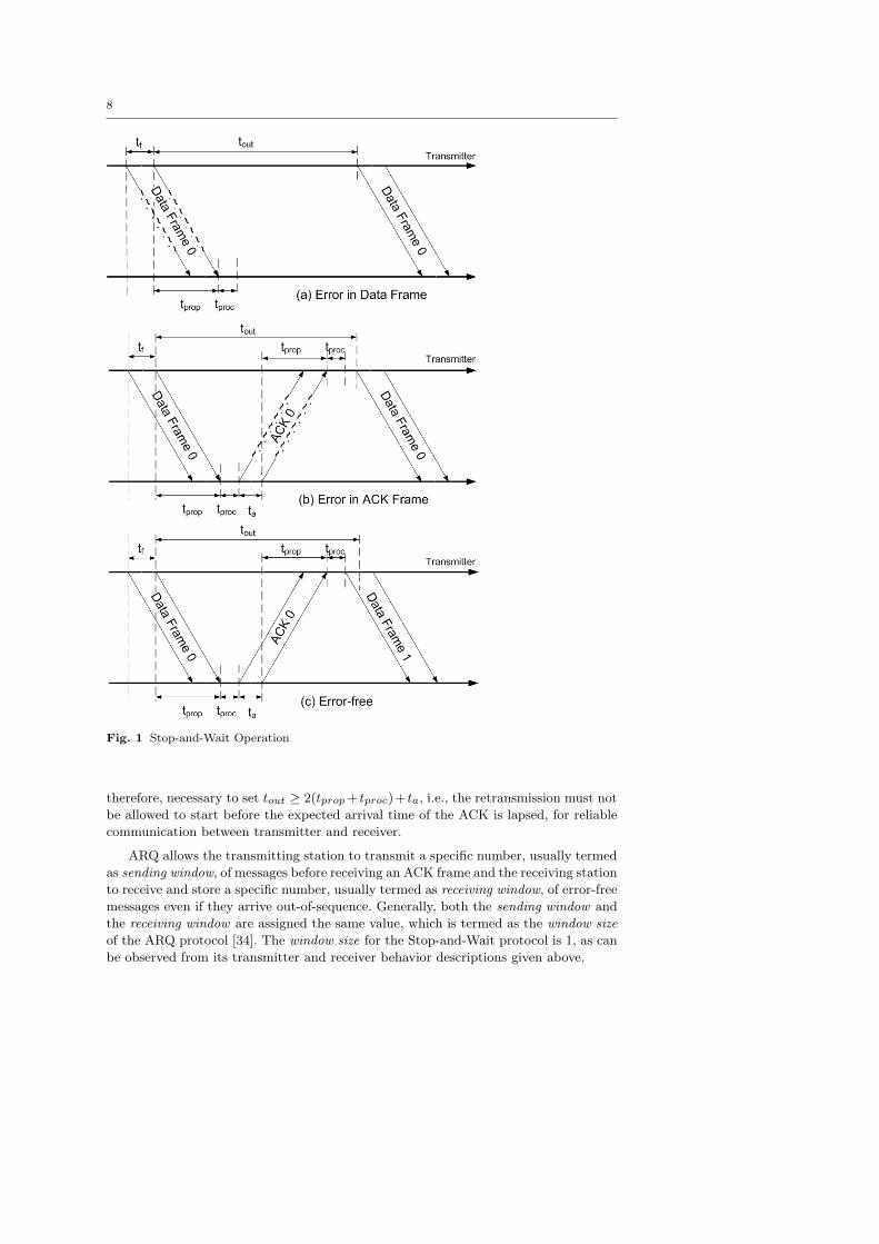
Fig. 1 using the following notation.

– tf : Data message transmission time

– ta: ACK message transmission time

– tprop: One-way signal propagation delay between transmitter and receiver

– tproc: Processing time required for error detection in the received message at both

transmitter and receiver

– tout: Timeout period

The transmitter sends a data message to the receiver and spends tf time units in

doing so. It then stops and waits to receive an acknowledgement (ACK) of reception

of that message from the receiver. If no ACK is received within a given time out, tout,

period, the data message is resent by the transmitter and once again it stops and starts

waiting for the ACK (Fig. 1.a). If an ACK is received within the given tout period then

the transmitter checks the received message for errors during the next tproc time units.

If errors are detected then the ACK is ignored and the data message is resent by the

transmitter after tout expires and once again the transmitter stops and waits for the

ACK (Fig. 1.b). Thus, the main idea is that the transmitter keeps on retransmitting

the same data message, after a pre-defined time-out period, tout, until and unless it

receives a corresponding error-free ACK message from the receiver. When an error-free

ACK message is finally received then the transmitter transmits the next data message

in its queue (Fig. 1.c).

The receiver is always waiting to receive data messages. When a new message

arrives, the receiver checks it for errors during the next tproc time units. If errors are

detected then the data message is ignored and the receiver continues to be in the wait

state (Fig. 1.a), otherwise it initiates the transmission of an ACK message, which takes

ta time units (Fig. 1.b,c).

Under the above mentioned conditions, the ACK message cannot be received before

tprop + tproc + ta + tprop + tproc units of time after sending out a data message. It is,

8

Fig. 1 Stop-and-Wait Operation

therefore, necessary to set tout ≥ 2(tprop + tproc)+ ta, i.e., the retransmission must not

be allowed to start before the expected arrival time of the ACK is lapsed, for reliable

communication between transmitter and receiver.

ARQ allows the transmitting station to transmit a specific number, usually termed

as sending window, of messages before receiving an ACK frame and the receiving station

to receive and store a specific number, usually termed as receiving window, of error-free

messages even if they arrive out-of-sequence. Generally, both the sending window and

the receiving window are assigned the same value, which is termed as the window size

of the ARQ protocol [34]. The window size for the Stop-and-Wait protocol is 1, as can

be observed from its transmitter and receiver behavior descriptions given above.

9

In order to distinguish between new messages and duplicates of previous messages

at the receiver or transmitter, a sequence number is included in the header of both data

and ACK messages [13]. It has been shown that, for correct ARQ operation, the number

of distinct sequence numbers must be at least equal to twice the window size [36]. Thus,

the simplest and the most commonly used version of the Stop-and-Wait protocol uses

two distinct sequence numbers (0 and 1) and is known as the ABP. The transmitter

keeps track of the sequence number of the last data message it had sent, its associated

timer and the message itself in case a retransmission is required. Whereas, the receiver

keeps track of the sequence number of the next data message that it is expecting to

receive. Thus, if an out-of-sequence data message arrives at the receiver, it ignores it

and responds with the ACK for the data message that it was expecting to receive. On

the other hand, when an in-sequence data message arrives at the receiver, it updates

its sequence number by performing a modulo-2 addition with the number 1, i.e., 0 is

updated to 1 and 1 is updated to 0 and responds using this updated sequence number.

Similarly, if an out-of-sequence ACK message appears at the transmitter, it ignores

it and retains the sequence number of the last data message it had sent. Whereas, in

the case of the reception of an in-sequence ACK message, the sequence number at the

transmitter is also updated by performing a modulo-2 addition by 1, which becomes

the sequence number of the next data message as well. More details about sequence

numbering in the Stop-and-Wait protocol can be found in [13].

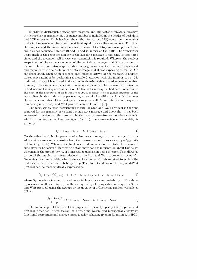
The most widely used performance metric for Stop-and-Wait protocol is the time

required for the transmitter to send a single data message and know that it has been

successfully received at the receiver. In the case of error-free or noiseless channels,

which do not reorder or lose messages (Fig. 1.c), the message transmission delay is

given by

tf + tprop + tproc + ta + tprop + tproc (4)

On the other hand, in the presence of noise, every damaged or lost message (data or

ACK) will cause a retransmission from the transmitter and thus wastes tf + tout units

of time (Fig. 1.a,b). Whereas, the final successful transmission will take the amount of

time given in Equation 4. In order to obtain more concise information about this delay,

we consider the probability, p, of a message transmission being in error. This allows us

to model the number of retransmissions in the Stop-and-Wait protocol in terms of a

Geometric random variable, which returns the number of trials required to achieve the

first success, with success probability 1− p. Therefore, the delay of the Stop-and-Wait

protocol can be mathematically expressed as

(tf + tout)(G(1−p) − 1) + tf + tprop + tproc + ta + tprop + tproc (5)

where Gx denotes a Geometric random variable with success probability x. The above

representation allows us to express the average delay of a single data message in a Stop-

and-Wait protocol using the average or mean value of a Geometric random variable as

follows

(tf + tout)p

1− p+ tf + tprop + tproc + ta + tprop + tproc (6)

The main scope of the rest of the paper is to formally specify the Stop-and-wait

protocol, described in this section, as a real-time system and mechanically verify its

functional correctness and average message delay relation, given in Equation 6, in HOL.

10

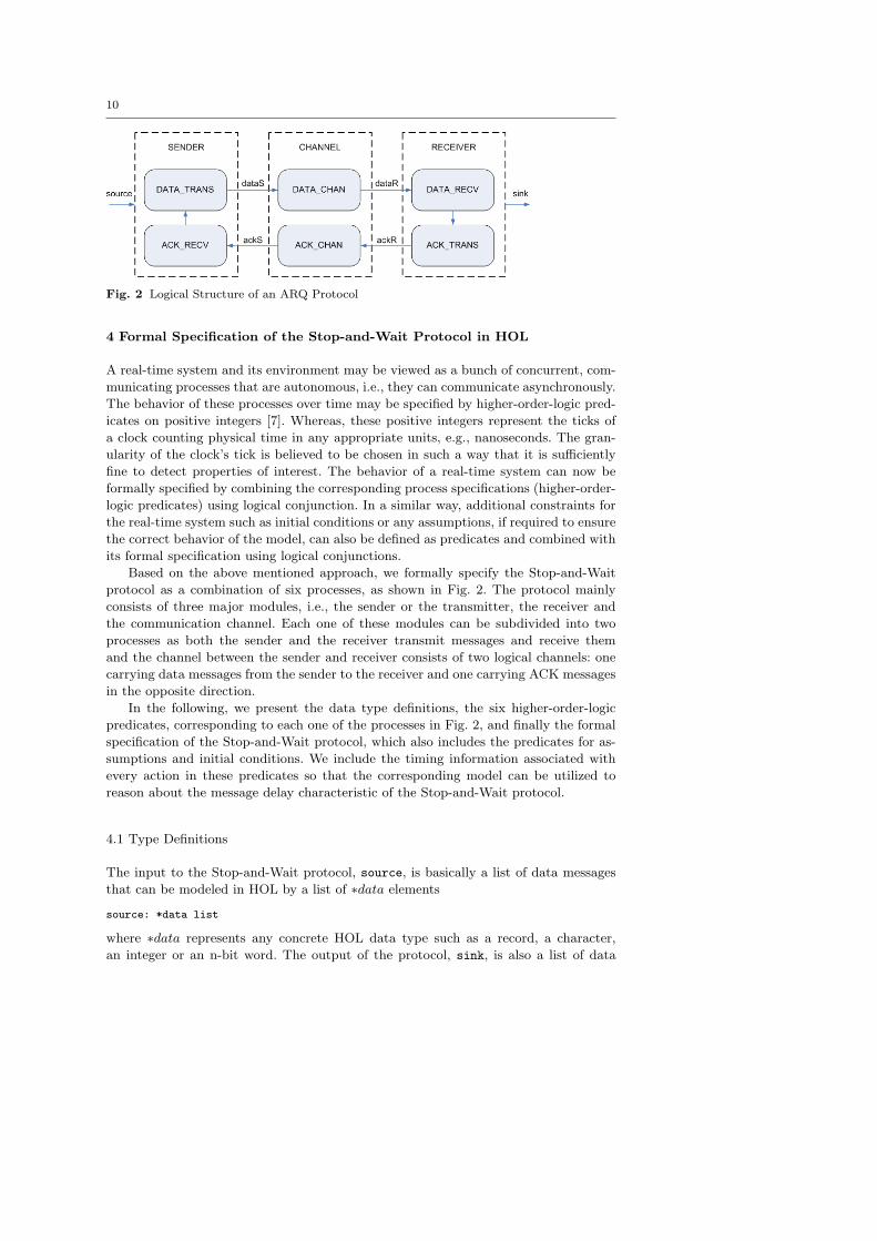
Fig. 2 Logical Structure of an ARQ Protocol

4 Formal Specification of the Stop-and-Wait Protocol in HOL

A real-time system and its environment may be viewed as a bunch of concurrent, com-

municating processes that are autonomous, i.e., they can communicate asynchronously.

The behavior of these processes over time may be specified by higher-order-logic pred-

icates on positive integers [7]. Whereas, these positive integers represent the ticks of

a clock counting physical time in any appropriate units, e.g., nanoseconds. The gran-

ularity of the clock’s tick is believed to be chosen in such a way that it is sufficiently

fine to detect properties of interest. The behavior of a real-time system can now be

formally specified by combining the corresponding process specifications (higher-order-

logic predicates) using logical conjunction. In a similar way, additional constraints for

the real-time system such as initial conditions or any assumptions, if required to ensure

the correct behavior of the model, can also be defined as predicates and combined with

its formal specification using logical conjunctions.

Based on the above mentioned approach, we formally specify the Stop-and-Wait

protocol as a combination of six processes, as shown in Fig. 2. The protocol mainly

consists of three major modules, i.e., the sender or the transmitter, the receiver and

the communication channel. Each one of these modules can be subdivided into two

processes as both the sender and the receiver transmit messages and receive them

and the channel between the sender and receiver consists of two logical channels: one

carrying data messages from the sender to the receiver and one carrying ACK messages

in the opposite direction.

In the following, we present the data type definitions, the six higher-order-logic

predicates, corresponding to each one of the processes in Fig. 2, and finally the formal

specification of the Stop-and-Wait protocol, which also includes the predicates for as-

sumptions and initial conditions. We include the timing information associated with

every action in these predicates so that the corresponding model can be utilized to

reason about the message delay characteristic of the Stop-and-Wait protocol.

4.1 Type Definitions

The input to the Stop-and-Wait protocol, source, is basically a list of data messages

that can be modeled in HOL by a list of ∗data elements

source: *data list

where ∗data represents any concrete HOL data type such as a record, a character,

an integer or an n-bit word. The output of the protocol, sink, is also a list of data

11

messages that grows with time as new data messages are delivered to the receiver. It

can be modeled in HOL as follows:

sink: time -> *data list

where time is assigned the HOL data-type for positive integers, num, and represents

physical time in this case. This kind of variable, which is time dependant, is termed as

a history in this paper.

The arrows in Fig. 2 between processes represent information that is shared between

the sender, channel and receiver. Data messages are transmitted from the sender to the

receiver (dataS, dataR) and ACK messages are transmitted in the opposite direction

(ackR, ackS). These messages are transmitted across the Stop-and-Wait protocol in

a form of a packet, which can be modeled in HOL as a pair containing a sequence

number and a message element

packet: num x *data

where num is used here for the sequence number and the ∗data represents the message.

Since we are dealing with an unreliable channel, the output of a channel may or may

not be a packet. In order to model the no-packet case in HOL, a data-type non packet

is defined, which has only one value, i.e., one. Every message can either be of type

packet or of type non packet.

message: packet + non_packet

4.2 Data Transmission

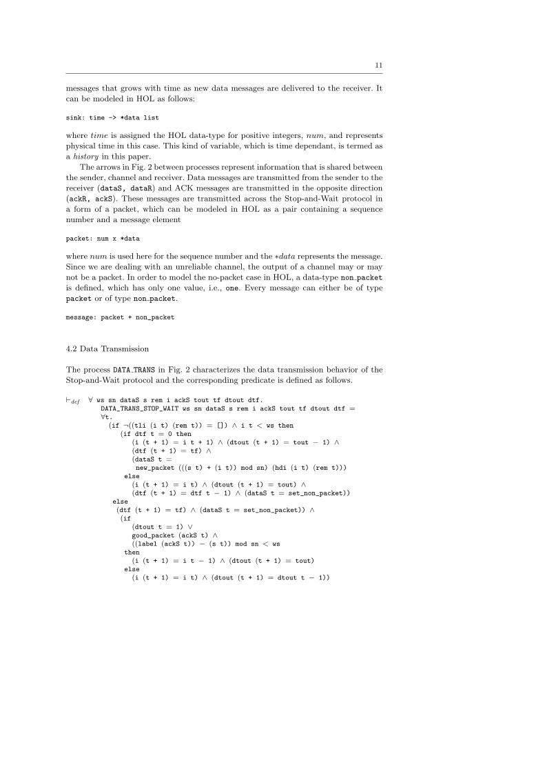
The process DATA TRANS in Fig. 2 characterizes the data transmission behavior of the

Stop-and-Wait protocol and the corresponding predicate is defined as follows.

`def ∀ ws sn dataS s rem i ackS tout tf dtout dtf.DATA_TRANS_STOP_WAIT ws sn dataS s rem i ackS tout tf dtout dtf =∀t.

(if ¬((tli (i t) (rem t)) = []) ∧ i t < ws then(if dtf t = 0 then

(i (t + 1) = i t + 1) ∧ (dtout (t + 1) = tout − 1) ∧(dtf (t + 1) = tf) ∧(dataS t =new_packet (((s t) + (i t)) mod sn) (hdi (i t) (rem t)))

else(i (t + 1) = i t) ∧ (dtout (t + 1) = tout) ∧(dtf (t + 1) = dtf t − 1) ∧ (dataS t = set_non_packet))

else(dtf (t + 1) = tf) ∧ (dataS t = set_non_packet)) ∧(if

(dtout t = 1) ∨good_packet (ackS t) ∧((label (ackS t)) − (s t)) mod sn < ws

then(i (t + 1) = i t − 1) ∧ (dtout (t + 1) = tout)

else(i (t + 1) = i t) ∧ (dtout (t + 1) = dtout t − 1))

12

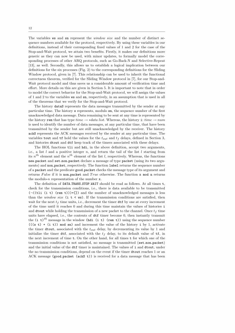
The variables ws and sn represent the window size and the number of distinct se-

quence numbers available for the protocol, respectively. By using these variables in our

definitions, instead of their corresponding fixed values of 1 and 2 for the case of the

Stop-and-Wait protocol, we attain two benefits. Firstly, it makes our definitions more

generic as they can now be used, with minor updates, to formally model the corre-

sponding processes of other ARQ protocols, such as Go-Back-N and Selective-Repeat

[13], as well. Secondly, this allows us to establish a logical implication between our

definitions for the six processes (Fig. 2) to the corresponding definitions for the Sliding

Window protocol, given in [7]. This relationship can be used to inherit the functional

correctness theorem, verified for the Sliding Window protocol in [7], for our Stop-and-

Wait protocol model and thus saves us a considerable amount of verification time and

effort. More details on this are given in Section 5. It is important to note that in order

to model the correct behavior for the Stop-and-Wait protocol, we will assign the values

of 1 and 2 to the variables ws and sn, respectively, in an assumption that is used in all

of the theorems that we verify for the Stop-and-Wait protocol.

The history dataS represents the data messages transmitted by the sender at any

particular time. The history s represents, modulo sn, the sequence number of the first

unacknowledged data message. Data remaining to be sent at any time is represented by

the history rem that has type time → ∗data list. Whereas, the history i: time → num

is used to identify the number of data messages, at any particular time, that have been

transmitted by the sender but are still unacknowledged by the receiver. The history

ackS represents the ACK messages received by the sender at any particular time. The

variables tout and tf hold the values for the tout and tf delays, defined in Section 3,

and histories dtout and dtf keep track of the timers associated with these delays.

The HOL functions tli and hdi, in the above definition, accept two arguments,

i.e., a list l and a positive integer n, and return the tail of the list l starting from

its nth element and the nth element of the list l, respectively. Whereas, the functions

new packet and set non packet declare a message of type packet (using its two argu-

ments) and non packet, respectively. The function label returns the sequence number

of a packet and the predicate good packet checks the message type of its argument and

returns False if it is non packet and True otherwise. The function x mod n returns

the modulo-n representation of the number x.

The definition of DATA TRANS STOP WAIT should be read as follows. At all times t,

check for the transmission conditions, i.e., there is data available to be transmitted

(¬((tli (i t) (rem t)))=[]) and the number of unacknowledged messages is less

than the window size (i t < ws). If the transmission conditions are satisfied, then

wait for the next tf time units, i.e., decrement the timer dtf by one at every increment

of the time until it reaches 0 and during this time maintain the values of histories i

and dtout while holding the transmission of a new packet to the channel. Once tf time

units have elapsed, i.e., the contents of dtf timer become 0, then instantly transmit

the (i t)th message in the window (hdi (i t) (rem t)) using the sequence number

(((s t) + (i t)) mod sn) and increment the value of the history i by 1, activate

the timer dtout, associated with the tout delay, by decrementing its value by 1 and

initialize the timer dtf, associated with the tf delay, to its default value of tf, in

the next increment of time t. On the other hand, for all times t for which one of the

transmission conditions is not satisfied, no message is transmitted (set non packet)

and the initial value of the dtf timer is maintained. The values of i and dtout, under

the no transmission conditions, depend on the event if the timer dtout reaches 1 or an

ACK message (good packet (ackS t)) is received for a data message that has been

13

sent and not yet acknowledged, i.e., if the difference between the label of (ackS t) and

the sender’s sequence number is less than ws ((label (ackS t)) - (s t) mod sn) <

ws). If this event happens, then the timer dtout is initialized to its default value tout

and the value of i is decremented by 1 in the next increment of time t. Otherwise,

we remain in the wait state until the timer dtout expires or a valid ACK is received,

while maintaining the value of i and decrementing the timer dtout by one at every

increment of the time t.

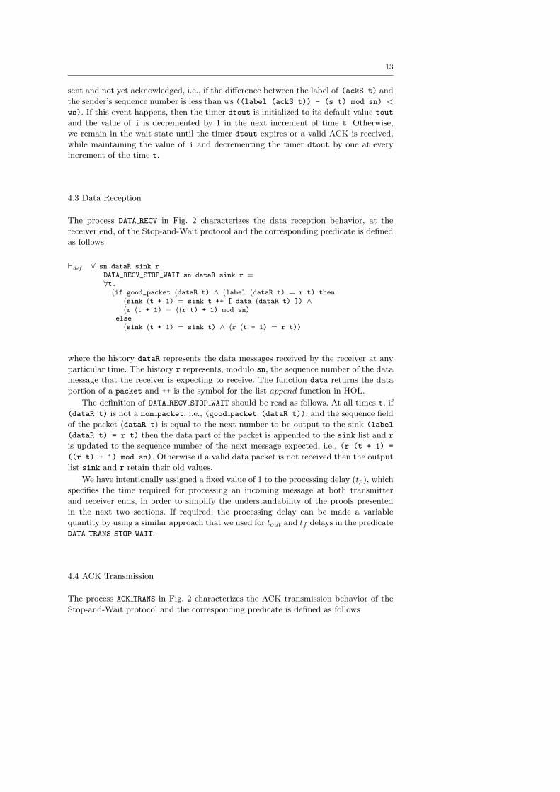
4.3 Data Reception

The process DATA RECV in Fig. 2 characterizes the data reception behavior, at the

receiver end, of the Stop-and-Wait protocol and the corresponding predicate is defined

as follows

`def ∀ sn dataR sink r.DATA_RECV_STOP_WAIT sn dataR sink r =∀t.

(if good_packet (dataR t) ∧ (label (dataR t) = r t) then(sink (t + 1) = sink t ++ [ data (dataR t) ]) ∧(r (t + 1) = ((r t) + 1) mod sn)

else(sink (t + 1) = sink t) ∧ (r (t + 1) = r t))

where the history dataR represents the data messages received by the receiver at any

particular time. The history r represents, modulo sn, the sequence number of the data

message that the receiver is expecting to receive. The function data returns the data

portion of a packet and ++ is the symbol for the list append function in HOL.

The definition of DATA RECV STOP WAIT should be read as follows. At all times t, if

(dataR t) is not a non packet, i.e., (good packet (dataR t)), and the sequence field

of the packet (dataR t) is equal to the next number to be output to the sink (label

(dataR t) = r t) then the data part of the packet is appended to the sink list and r

is updated to the sequence number of the next message expected, i.e., (r (t + 1) =

((r t) + 1) mod sn). Otherwise if a valid data packet is not received then the output

list sink and r retain their old values.

We have intentionally assigned a fixed value of 1 to the processing delay (tp), which

specifies the time required for processing an incoming message at both transmitter

and receiver ends, in order to simplify the understandability of the proofs presented

in the next two sections. If required, the processing delay can be made a variable

quantity by using a similar approach that we used for tout and tf delays in the predicate

DATA TRANS STOP WAIT.

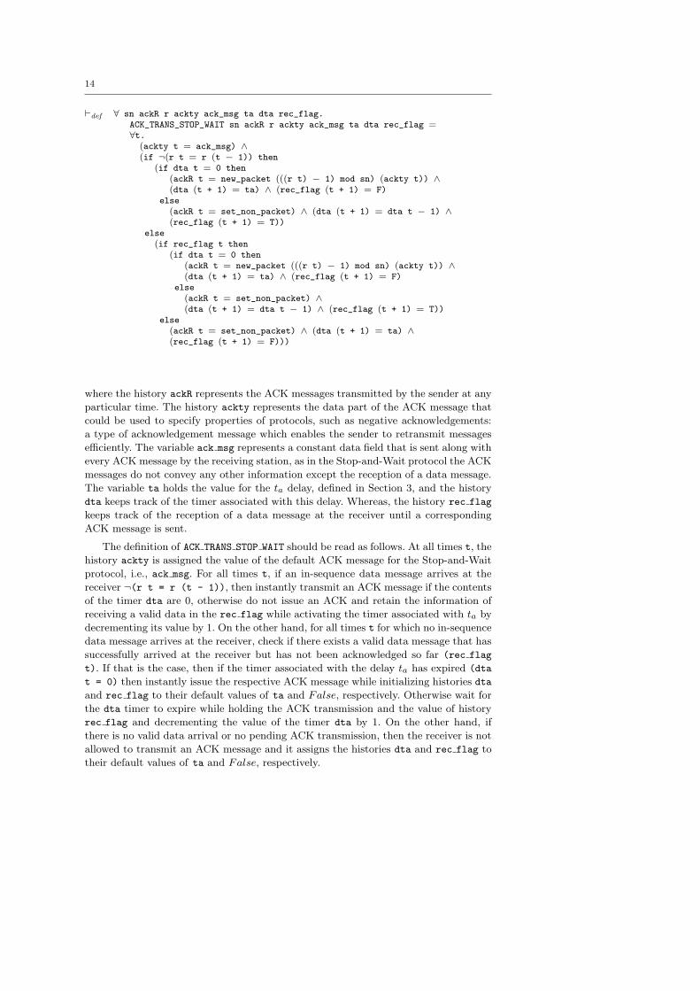
4.4 ACK Transmission

The process ACK TRANS in Fig. 2 characterizes the ACK transmission behavior of the

Stop-and-Wait protocol and the corresponding predicate is defined as follows

14

`def ∀ sn ackR r ackty ack_msg ta dta rec_flag.ACK_TRANS_STOP_WAIT sn ackR r ackty ack_msg ta dta rec_flag =∀t.

(ackty t = ack_msg) ∧(if ¬(r t = r (t − 1)) then

(if dta t = 0 then(ackR t = new_packet (((r t) − 1) mod sn) (ackty t)) ∧(dta (t + 1) = ta) ∧ (rec_flag (t + 1) = F)

else(ackR t = set_non_packet) ∧ (dta (t + 1) = dta t − 1) ∧(rec_flag (t + 1) = T))

else(if rec_flag t then

(if dta t = 0 then(ackR t = new_packet (((r t) − 1) mod sn) (ackty t)) ∧(dta (t + 1) = ta) ∧ (rec_flag (t + 1) = F)

else(ackR t = set_non_packet) ∧(dta (t + 1) = dta t − 1) ∧ (rec_flag (t + 1) = T))

else(ackR t = set_non_packet) ∧ (dta (t + 1) = ta) ∧(rec_flag (t + 1) = F)))

where the history ackR represents the ACK messages transmitted by the sender at any

particular time. The history ackty represents the data part of the ACK message that

could be used to specify properties of protocols, such as negative acknowledgements:

a type of acknowledgement message which enables the sender to retransmit messages

efficiently. The variable ack msg represents a constant data field that is sent along with

every ACK message by the receiving station, as in the Stop-and-Wait protocol the ACK

messages do not convey any other information except the reception of a data message.

The variable ta holds the value for the ta delay, defined in Section 3, and the history

dta keeps track of the timer associated with this delay. Whereas, the history rec flag

keeps track of the reception of a data message at the receiver until a corresponding

ACK message is sent.

The definition of ACK TRANS STOP WAIT should be read as follows. At all times t, the

history ackty is assigned the value of the default ACK message for the Stop-and-Wait

protocol, i.e., ack msg. For all times t, if an in-sequence data message arrives at the

receiver ¬(r t = r (t - 1)), then instantly transmit an ACK message if the contents

of the timer dta are 0, otherwise do not issue an ACK and retain the information of

receiving a valid data in the rec flag while activating the timer associated with ta by

decrementing its value by 1. On the other hand, for all times t for which no in-sequence

data message arrives at the receiver, check if there exists a valid data message that has

successfully arrived at the receiver but has not been acknowledged so far (rec flag

t). If that is the case, then if the timer associated with the delay ta has expired (dta

t = 0) then instantly issue the respective ACK message while initializing histories dta

and rec flag to their default values of ta and False, respectively. Otherwise wait for

the dta timer to expire while holding the ACK transmission and the value of history

rec flag and decrementing the value of the timer dta by 1. On the other hand, if

there is no valid data arrival or no pending ACK transmission, then the receiver is not

allowed to transmit an ACK message and it assigns the histories dta and rec flag to

their default values of ta and False, respectively.

15

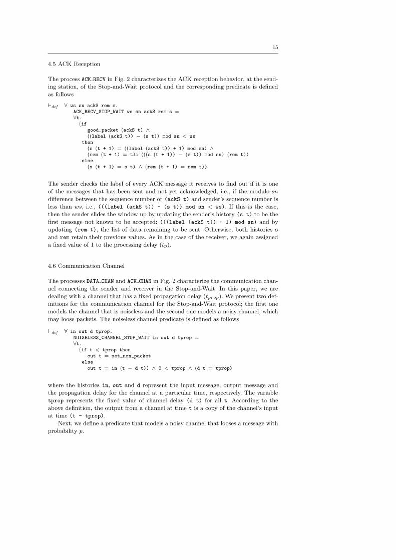
4.5 ACK Reception

The process ACK RECV in Fig. 2 characterizes the ACK reception behavior, at the send-

ing station, of the Stop-and-Wait protocol and the corresponding predicate is defined

as follows

`def ∀ ws sn ackS rem s.ACK_RECV_STOP_WAIT ws sn ackS rem s =∀t.

(ifgood_packet (ackS t) ∧((label (ackS t)) − (s t)) mod sn < ws

then(s (t + 1) = ((label (ackS t)) + 1) mod sn) ∧(rem (t + 1) = tli (((s (t + 1)) − (s t)) mod sn) (rem t))

else(s (t + 1) = s t) ∧ (rem (t + 1) = rem t))

The sender checks the label of every ACK message it receives to find out if it is one

of the messages that has been sent and not yet acknowledged, i.e., if the modulo-sn

difference between the sequence number of (ackS t) and sender’s sequence number is

less than ws, i.e., (((label (ackS t)) - (s t)) mod sn < ws). If this is the case,

then the sender slides the window up by updating the sender’s history (s t) to be the

first message not known to be accepted: (((label (ackS t)) + 1) mod sn) and by

updating (rem t), the list of data remaining to be sent. Otherwise, both histories s

and rem retain their previous values. As in the case of the receiver, we again assigned

a fixed value of 1 to the processing delay (tp).

4.6 Communication Channel

The processes DATA CHAN and ACK CHAN in Fig. 2 characterize the communication chan-

nel connecting the sender and receiver in the Stop-and-Wait. In this paper, we are

dealing with a channel that has a fixed propagation delay (tprop). We present two def-

initions for the communication channel for the Stop-and-Wait protocol; the first one

models the channel that is noiseless and the second one models a noisy channel, which

may loose packets. The noiseless channel predicate is defined as follows

`def ∀ in out d tprop.NOISELESS_CHANNEL_STOP_WAIT in out d tprop =∀t.

(if t < tprop thenout t = set_non_packet

elseout t = in (t − d t)) ∧ 0 < tprop ∧ (d t = tprop)

where the histories in, out and d represent the input message, output message and

the propagation delay for the channel at a particular time, respectively. The variable

tprop represents the fixed value of channel delay (d t) for all t. According to the

above definition, the output from a channel at time t is a copy of the channel’s input

at time (t - tprop).

Next, we define a predicate that models a noisy channel that looses a message with

probability p.

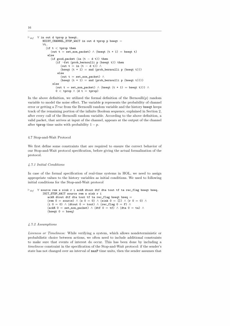
16

`def ∀ in out d tprop p bseqt.NOISY_CHANNEL_STOP_WAIT in out d tprop p bseqt =∀t.

(if t < tprop then(out t = set_non_packet) ∧ (bseqt (t + 1) = bseqt t)

else(if good_packet (in (t − d t)) then

(if ¬fst (prob_bernoulli p (bseqt t)) then(out t = in (t − d t)) ∧(bseqt (t + 1) = snd (prob_bernoulli p (bseqt t)))

else(out t = set_non_packet) ∧(bseqt (t + 1) = snd (prob_bernoulli p (bseqt t))))

else(out t = set_non_packet) ∧ (bseqt (t + 1) = bseqt t))) ∧0 < tprop ∧ (d t = tprop)

In the above definition, we utilized the formal definition of the Bernoulli(p) random

variable to model the noise effect. The variable p represents the probability of channel

error or getting a True from the Bernoulli random variable and the history bseqt keeps

track of the remaining portion of the infinite Boolean sequence, explained in Section 2,

after every call of the Bernoulli random variable. According to the above definition, a

valid packet, that arrives at input of the channel, appears at the output of the channel

after tprop time units with probability 1− p.

4.7 Stop-and-Wait Protocol

We first define some constraints that are required to ensure the correct behavior of

our Stop-and-Wait protocol specification, before giving the actual formalization of the

protocol.

4.7.1 Initial Conditions

In case of the formal specification of real-time systems in HOL, we need to assign

appropriate values to the history variables as initial conditions. We used to following

initial conditions for the Stop-and-Wait protocol

`def ∀ source rem s sink r i ackR dtout dtf dta tout tf ta rec_flag bseqt bseq.INIT_STOP_WAIT source rem s sink r i

ackR dtout dtf dta tout tf ta rec_flag bseqt bseq =(rem 0 = source) ∧ (s 0 = 0) ∧ (sink 0 = []) ∧ (r 0 = 0) ∧(i 0 = 0) ∧ (dtout 0 = tout) ∧ (rec_flag 0 = F) ∧(ackR 0 = set_non_packet) ∧ (dtf 0 = tf) ∧ (dta 0 = ta) ∧(bseqt 0 = bseq)

4.7.2 Assumptions

Liveness or Timeliness: While verifying a system, which allows nondeterministic or

probabilistic choice between actions, we often need to include additional constraints

to make sure that events of interest do occur. This has been done by including a

timeliness constraint in the specification of the Stop-and-Wait protocol: if the sender’s

state has not changed over an interval of maxP time units, then the sender assumes that

17

the receiver or the channel has crashed and aborts the protocol. A predicate ABORT is

defined that is True only when the protocol aborts and False otherwise. Now, the

predicate ABORT characterizes which abort histories satisfy this constraint.

`def ∀ abort maxP rem.ABORT abort maxP rem =∀t.abort t = (rem t = rem (t − maxP)) ∧ maxP ≤ t ∧ ¬(rem t = [])

A protocol is said to be live if it is never aborted. This kind of liveness is assumed

using the following constraint

LIVE_ASSUMPTION abort = ∀ t. ¬(abort t)

Window Size and Sequence Numbers: As has been mentioned before, instead of using

their exact values of 1 and 2, we used variables ws and sn to represent the window size

and distinct sequence numbers for the Stop-and-Wait protocol in the above predicates.

This has been done, in order to be able to establish logical implication between the

predicates defined in this paper and the corresponding predicates for the Sliding Win-

dow protocol, defined in [7]. Now, we assign the exact values to these variables in an

assumption predicate as follows

`def ∀ ws sn.WSSN_ASSUM_STOP_WAIT ws sn = (ws = 1) ∧ (sn = 2)

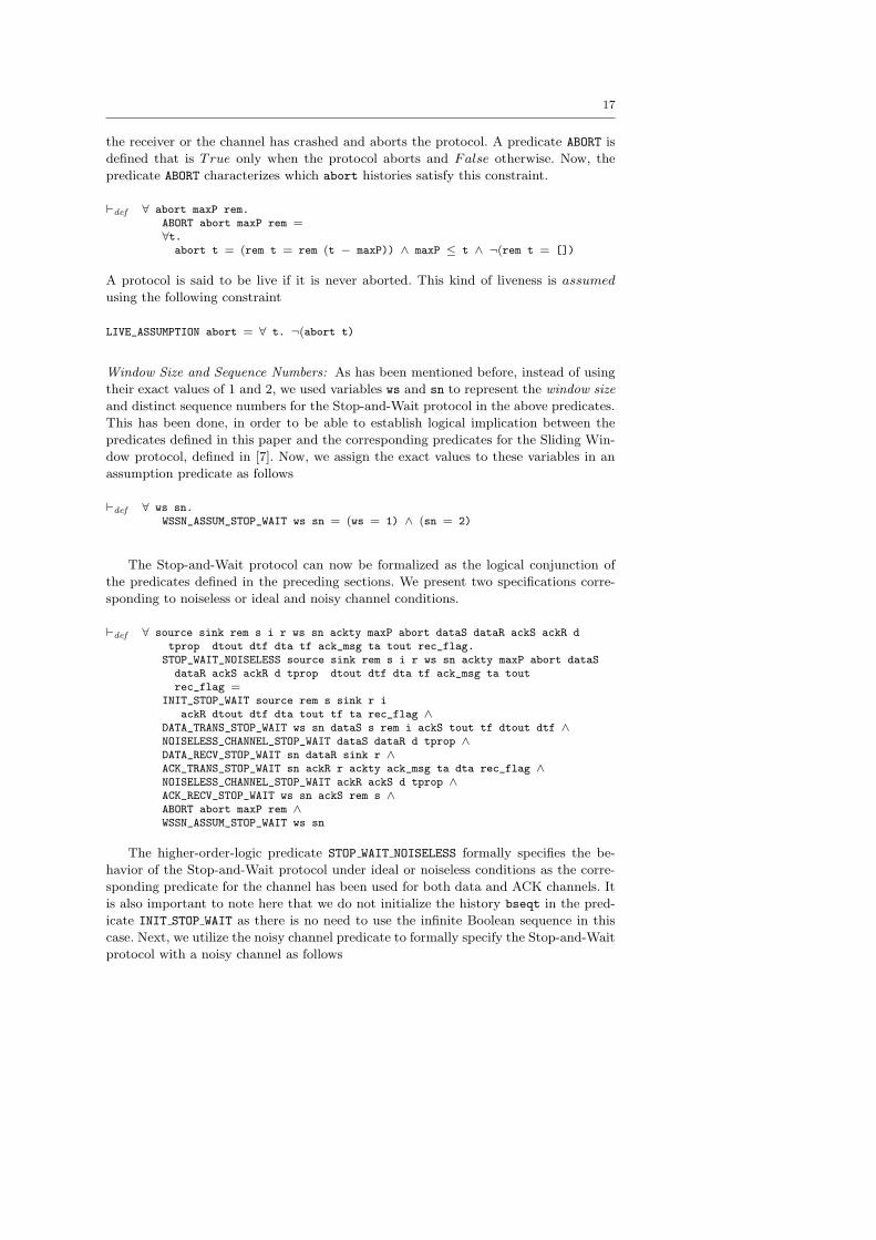
The Stop-and-Wait protocol can now be formalized as the logical conjunction of

the predicates defined in the preceding sections. We present two specifications corre-

sponding to noiseless or ideal and noisy channel conditions.

`def ∀ source sink rem s i r ws sn ackty maxP abort dataS dataR ackS ackR dtprop dtout dtf dta tf ack_msg ta tout rec_flag.STOP_WAIT_NOISELESS source sink rem s i r ws sn ackty maxP abort dataSdataR ackS ackR d tprop dtout dtf dta tf ack_msg ta toutrec_flag =

INIT_STOP_WAIT source rem s sink r iackR dtout dtf dta tout tf ta rec_flag ∧

DATA_TRANS_STOP_WAIT ws sn dataS s rem i ackS tout tf dtout dtf ∧NOISELESS_CHANNEL_STOP_WAIT dataS dataR d tprop ∧DATA_RECV_STOP_WAIT sn dataR sink r ∧ACK_TRANS_STOP_WAIT sn ackR r ackty ack_msg ta dta rec_flag ∧NOISELESS_CHANNEL_STOP_WAIT ackR ackS d tprop ∧ACK_RECV_STOP_WAIT ws sn ackS rem s ∧ABORT abort maxP rem ∧WSSN_ASSUM_STOP_WAIT ws sn

The higher-order-logic predicate STOP WAIT NOISELESS formally specifies the be-

havior of the Stop-and-Wait protocol under ideal or noiseless conditions as the corre-

sponding predicate for the channel has been used for both data and ACK channels. It

is also important to note here that we do not initialize the history bseqt in the pred-

icate INIT STOP WAIT as there is no need to use the infinite Boolean sequence in this

case. Next, we utilize the noisy channel predicate to formally specify the Stop-and-Wait

protocol with a noisy channel as follows

18

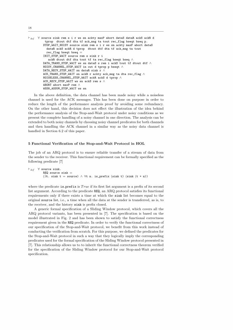
`def ∀ source sink rem s i r ws sn ackty maxP abort dataS dataR ackS ackR dtprop dtout dtf dta tf ack_msg ta tout rec_flag bseqt bseq p.STOP_WAIT_NOISY source sink rem s i r ws sn ackty maxP abort dataSdataR ackS ackR d tprop dtout dtf dta tf ack_msg ta toutrec_flag bseqt bseq =

INIT_STOP_WAIT source rem s sink r iackR dtout dtf dta tout tf ta rec_flag bseqt bseq ∧

DATA_TRANS_STOP_WAIT ws sn dataS s rem i ackS tout tf dtout dtf ∧NOISY_CHANNEL_STOP_WAIT in out d tprop p bseqt ∧DATA_RECV_STOP_WAIT sn dataR sink r ∧ACK_TRANS_STOP_WAIT sn ackR r ackty ack_msg ta dta rec_flag ∧NOISELESS_CHANNEL_STOP_WAIT ackR ackS d tprop ∧ACK_RECV_STOP_WAIT ws sn ackS rem s ∧ABORT abort maxP rem ∧WSSN_ASSUM_STOP_WAIT ws sn

In the above definition, the data channel has been made noisy while a noiseless

channel is used for the ACK messages. This has been done on purpose in order to

reduce the length of the performance analysis proof by avoiding some redundancy.

On the other hand, this decision does not effect the illustration of the idea behind

the performance analysis of the Stop-and-Wait protocol under noisy conditions as we

present the complete handling of a noisy channel in one direction. The analysis can be

extended to both noisy channels by choosing noisy channel predicates for both channels

and then handling the ACK channel in a similar way as the noisy data channel is

handled in Section 6.2 of this paper.

5 Functional Verification of the Stop-and-Wait Protocol in HOL

The job of an ARQ protocol is to ensure reliable transfer of a stream of data from

the sender to the receiver. This functional requirement can be formally specified as the

following predicate [7]

`def ∀ source sink.REQ source sink =(∃t. sink t = source) ∧ ∀t n. is_prefix (sink t) (sink (t + n))

where the predicate is prefix is True if its first list argument is a prefix of its second

list argument. According to the predicate REQ, an ARQ protocol satisfies its functional

requirements only if there exists a time at which the sink list becomes equal to the

original source list, i.e., a time when all the data at the sender is transferred, as is, to

the receiver, and the history sink is prefix closed.

A generic formal specification of a Sliding Window protocol, which covers all the

ARQ protocol variants, has been presented in [7]. The specification is based on the

model illustrated in Fig. 2 and has been shown to satisfy the functional correctness

requirement given in the REQ predicate. In order to verify the functional correctness of

our specification of the Stop-and-Wait protocol, we benefit from this work instead of

conducting the verification from scratch. For this purpose, we defined the predicates for

the Stop-and-Wait protocol in such a way that they logically imply the corresponding

predicates used for the formal specification of the Sliding Window protocol presented in

[7]. This relationship allows us to to inherit the functional correctness theorem verified

for the specification of the Sliding Window protocol for our Stop-and-Wait protocol

specification.

19

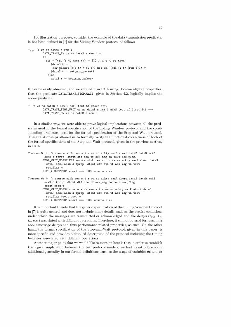
For illustration purposes, consider the example of the data transmission predicate.

It has been defined in [7] for the Sliding Window protocol as follows

`def ∀ ws sn dataS s rem i.DATA_TRANS_SW ws sn dataS s rem i =∀t.

(if ¬((tli (i t) (rem t)) = []) ∧ i t < ws then(dataS t =new_packet (((s t) + (i t)) mod sn) (hdi (i t) (rem t))) ∨

(dataS t = set_non_packet)elsedataS t = set_non_packet)

It can be easily observed, and we verified it in HOL using Boolean algebra properties,

that the predicate DATA TRANS STOP WAIT, given in Section 4.2, logically implies the

above predicate

` ∀ ws ns dataS s rem i ackS tout tf dtout dtf.DATA_TRANS_STOP_WAIT ws ns dataS s rem i ackS tout tf dtout dtf =⇒DATA_TRANS_SW ws ns dataS s rem i

In a similar way, we were able to prove logical implications between all the pred-

icates used in the formal specification of the Sliding Window protocol and the corre-

sponding predicates used for the formal specification of the Stop-and-Wait protocol.

These relationships allowed us to formally verify the functional correctness of both of

the formal specifications of the Stop-and-Wait protocol, given in the previous section,

in HOL.

Theorem 5: ` ∀ source sink rem s i r ws sn ackty maxP abort dataS dataR ackSackR d tprop dtout dtf dta tf ack_msg ta tout rec_flag.STOP_WAIT_NOISELESS source sink rem s i r ws sn ackty maxP abort dataSdataR ackS ackR d tprop dtout dtf dta tf ack_msg ta toutrec_flag ∧

LIVE_ASSUMPTION abort =⇒ REQ source sink

Theorem 6: ` ∀ source sink rem s i r ws sn ackty maxP abort dataS dataR ackSackR d tprop dtout dtf dta tf ack_msg ta tout rec_flagbseqt bseq p.STOP_WAIT_NOISY source sink rem s i r ws sn ackty maxP abort dataSdataR ackS ackR d tprop dtout dtf dta tf ack_msg ta toutrec_flag bseqt bseq ∧

LIVE_ASSUMPTION abort =⇒ REQ source sink

It is important to note that the generic specification of the Sliding Window Protocol

in [7] is quite general and does not include many details, such as the precise conditions

under which the messages are transmitted or acknowledged and the delays (tout, tf ,

ta, etc.) associated with different operations. Therefore, it cannot be used for reasoning

about message delays and thus performance related properties, as such. On the other

hand, the formal specification of the Stop-and-Wait protocol, given in this paper, is

more specific and provides a detailed description of the protocol including the timing

behavior associated with different operations.

Another major point that we would like to mention here is that in order to establish

the logical implication between the two protocol models, we had to introduce some

additional generality in our formal definitions, such as the usage of variables ws and sn

20

instead of their exact values of 1 and 2 , respectively. Even though, such generalizations

are not required for the functional description of the Stop-and-Wait protocol, they do

not harm us in any way. They lead to a much faster functional verification, as has been

illustrated in this section. On the other hand, they do not effect the formal reasoning

related to the performance issues, since the exact values for these variables are assigned

in an assumption (WSSN ASSUM STOP WAIT) that is a part of our Stop-and-Wait protocol

specification, which is used for conducting performance analysis.

6 Performance Analysis of the Stop-and-Wait Protocol

In this section, we present the verification of the message delay relations for the Stop-

and-Wait protocol, given in Equations 4 and 6, for noiseless and noisy channels, respec-

tively. The verification is based on the two formal specifications of the Stop-and-Wait

protocol, STOP WAIT NOISELESS and STOP WAIT NOISY, given in Section 4.

6.1 Noiseless Channel Conditions

The first and the foremost step in verifying the message delay characteristic for the

Stop-and-Wait protocol is to formally specify it. Informally speaking, the message delay

refers to the time required for the transmitter to send a single data message and know

that it has been successfully received at the receiver. We specify this in higher-order-

logic as follows

`def ∀ rem source.DELAY_STOP_WAIT_NOISELESS rem source =@t. (rem t = TL source) ∧ (rem (t − 1) = source)

where TL refers to the tail function for lists and @x.t refers to the Hilbert choice

operator in HOL (εx.t term) that represents the value of x such that t is True. Thus,

the above specification returns the time t at which the rem list, which represents the

data remaining to be sent at any time t, is reduced by one element from its initially

assigned value of the source list. Indeed it is precisely equal to the message delay of

the first data element in the source list.

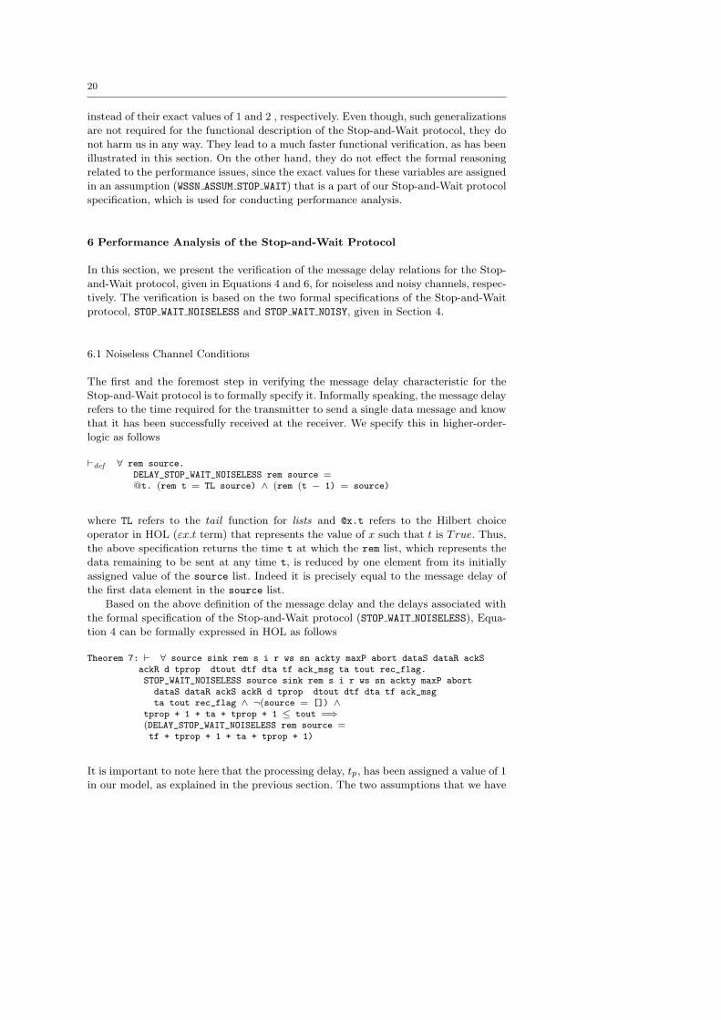
Based on the above definition of the message delay and the delays associated with

the formal specification of the Stop-and-Wait protocol (STOP WAIT NOISELESS), Equa-

tion 4 can be formally expressed in HOL as follows

Theorem 7: ` ∀ source sink rem s i r ws sn ackty maxP abort dataS dataR ackSackR d tprop dtout dtf dta tf ack_msg ta tout rec_flag.STOP_WAIT_NOISELESS source sink rem s i r ws sn ackty maxP abort

dataS dataR ackS ackR d tprop dtout dtf dta tf ack_msgta tout rec_flag ∧ ¬(source = []) ∧

tprop + 1 + ta + tprop + 1 ≤ tout =⇒(DELAY_STOP_WAIT_NOISELESS rem source =tf + tprop + 1 + ta + tprop + 1)

It is important to note here that the processing delay, tp, has been assigned a value of 1

in our model, as explained in the previous section. The two assumptions that we have

21

added to Theorem 7 ensure that the source list is not an empty list, i.e., ¬(source =

[]), otherwise no data transfer takes place, and the time out period tout is always

greater than or equal to its lower bound specified in Section 3.

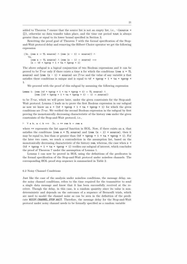
Rewriting the proof goal of Theorem 7 with the formal specification of the Stop-

and-Wait protocol delay and removing the Hilbert Choice operator we get the following

expression

(∃x. (rem x = TL source) ∧ (rem (x − 1) = source)) ∧∀x.

(rem x = TL source) ∧ (rem (x − 1) = source) =⇒(x = tf + tprop + 1 + ta + tprop + 1)

The above subgoal is a logical conjunction of two Boolean expressions and it can be

proved to be True only if there exists a time x for which the conditions (rem x = TL

source) and (rem (x - 1) = source) are True and the value of any variable x that

satisfies these conditions is unique and is equal to tf + tprop + 1 + ta + tprop +

1.

We proceed with the proof of this subgoal by assuming the following expression

Lemma 1: (rem (tf + tprop + 1 + ta + tprop + 1) = TL source) ∧(rem ((tf + tprop + 1 + ta + tprop + 1) − 1) = source))

to be True, which we will prove later, under the given constraints for the Stop-and-

Wait protocol. Lemma 1 leads us to prove the first Boolean expression in our subgoal

as now we know an x = (tf + tprop + 1 + ta + tprop + 1) for which the given

conditions are True. We verified the second Boolean expression in the subgoal by first

proving the monotonically decreasing characteristic of the history rem under the given

constraints of the Stop-and-Wait protocol, i.e.,

` ∀ a b. a < b =⇒ ∃c. c ++ rem b = rem a

where ++ represents the list append function in HOL. Now, if there exists an x, that

satisfies the conditions (rem x = TL source) and (rem (x - 1) = source), then it

may be equal to, less than or greater than (tf + tprop + 1 + ta + tprop + 1). For

the later two cases, we reach a contradiction in the assumption list, based on the

monotonically decreasing characteristic of the history rem, whereas, the case when x =

(tf + tprop + 1 + ta + tprop + 1) verifies our subgoal of interest, which concludes

the proof of Theorem 7 under the assumption of Lemma 1.

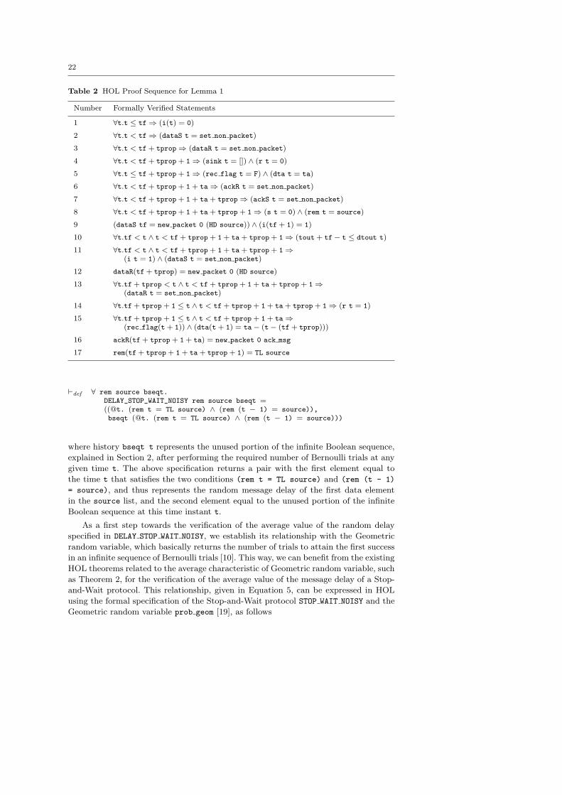
Lemma 1 can now be proved in HOL using the definitions of the predicates in

the formal specification of the Stop-and-Wait protocol under noiseless channels. The

corresponding HOL proof step sequence is summarized in Table 2.

6.2 Noisy Channel Conditions

Just like the case of the analysis under noiseless conditions, the message delay, un-

der noisy channel conditions, refers to the time required for the transmitter to send

a single data message and know that it has been successfully received at the re-

ceiver. Though the delay, in this case, is a random quantity since its value is non-

deterministic and depends on the outcomes of a sequence of Bernoulli trials, which

are used to model the channel noise as can be seen in the definition of the predi-

cate NOISY CHANNEL STOP WAIT. Therefore, the message delay for the Stop-and-Wait

protocol under noisy channel needs to be formally specified as a random variable

22

Table 2 HOL Proof Sequence for Lemma 1

Number Formally Verified Statements

1 ∀t.t ≤ tf⇒ (i(t) = 0)

2 ∀t.t < tf⇒ (dataS t = set non packet)

3 ∀t.t < tf + tprop⇒ (dataR t = set non packet)

4 ∀t.t < tf + tprop + 1⇒ (sink t = []) ∧ (r t = 0)

5 ∀t.t ≤ tf + tprop + 1⇒ (rec flag t = F) ∧ (dta t = ta)

6 ∀t.t < tf + tprop + 1 + ta⇒ (ackR t = set non packet)

7 ∀t.t < tf + tprop + 1 + ta + tprop⇒ (ackS t = set non packet)

8 ∀t.t < tf + tprop + 1 + ta + tprop + 1⇒ (s t = 0) ∧ (rem t = source)

9 (dataS tf = new packet 0 (HD source)) ∧ (i(tf + 1) = 1)

10 ∀t.tf < t ∧ t < tf + tprop + 1 + ta + tprop + 1⇒ (tout + tf− t ≤ dtout t)

11 ∀t.tf < t ∧ t < tf + tprop + 1 + ta + tprop + 1⇒(i t = 1) ∧ (dataS t = set non packet)

12 dataR(tf + tprop) = new packet 0 (HD source)

13 ∀t.tf + tprop < t ∧ t < tf + tprop + 1 + ta + tprop + 1⇒(dataR t = set non packet)

14 ∀t.tf + tprop + 1 ≤ t ∧ t < tf + tprop + 1 + ta + tprop + 1⇒ (r t = 1)

15 ∀t.tf + tprop + 1 ≤ t ∧ t < tf + tprop + 1 + ta⇒(rec flag(t + 1)) ∧ (dta(t + 1) = ta− (t− (tf + tprop)))

16 ackR(tf + tprop + 1 + ta) = new packet 0 ack msg

17 rem(tf + tprop + 1 + ta + tprop + 1) = TL source

`def ∀ rem source bseqt.DELAY_STOP_WAIT_NOISY rem source bseqt =((@t. (rem t = TL source) ∧ (rem (t − 1) = source)),bseqt (@t. (rem t = TL source) ∧ (rem (t − 1) = source)))

where history bseqt t represents the unused portion of the infinite Boolean sequence,

explained in Section 2, after performing the required number of Bernoulli trials at any

given time t. The above specification returns a pair with the first element equal to

the time t that satisfies the two conditions (rem t = TL source) and (rem (t - 1)

= source), and thus represents the random message delay of the first data element

in the source list, and the second element equal to the unused portion of the infinite

Boolean sequence at this time instant t.

As a first step towards the verification of the average value of the random delay

specified in DELAY STOP WAIT NOISY, we establish its relationship with the Geometric

random variable, which basically returns the number of trials to attain the first success

in an infinite sequence of Bernoulli trials [10]. This way, we can benefit from the existing

HOL theorems related to the average characteristic of Geometric random variable, such

as Theorem 2, for the verification of the average value of the message delay of a Stop-

and-Wait protocol. This relationship, given in Equation 5, can be expressed in HOL

using the formal specification of the Stop-and-Wait protocol STOP WAIT NOISY and the

Geometric random variable prob geom [19], as follows

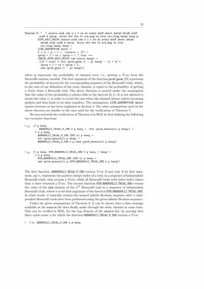
23

Theorem 8: ` ∀ source sink rem s i r ws sn ackty maxP abort dataS dataR ackSackR d tprop dtout dtf dta tf ack_msg ta tout rec_flag bseqt bseq p.STOP_WAIT_NOISY source sink rem s i r ws sn ackty maxP abort dataSdataR ackS ackR d tprop dtout dtf dta tf ack_msg ta toutrec_flag bseqt bseq ∧

LIVE_ASSUMPTION abort ∧0 ≤ p ∧ p < 1 ∧ ¬(source = []) ∧tprop + 1 + ta + tprop + 1 ≤ tout =⇒(DELAY_STOP_WAIT_NOISY rem source bseqt =((tf + tout) * (fst (prob_geom (1 − p) bseq) − 1) + tf +tprop + 1 + ta + tprop + 1,snd (prob_geom (1 − p) bseq)))

where p represents the probability of channel error, i.e., getting a True from the

Bernoulli random variable. The first argument of the function prob geom [19] represents

the probability of success for the corresponding sequence of the Bernoulli trials, which,

in the case of our definition of the noisy channel, is equal to the probability of getting

a False from a Bernoulli trial. The above theorem is proved under the assumption

that the value of the probability p always falls in the interval [0, 1). It is not allowed to

attain the value 1, in order to avoid the case when the channel always rejects incoming

packets and thus leads to no data transfers. The assumption, LIVE ASSUMPTION abort

ensures liveness as has been explained in Section 4. The other assumptions used in the

above theorem are similar to the ones used for the verification of Theorem 7.

We proceed with the verification of Theorem 8 in HOL by first defining the following

two recursive functions

`def (∀ p bseq.BERNOULLI_TRIAL_F_IND 0 p bseq = ¬fst (prob_bernoulli p bseq)) ∧

∀ n p bseq.BERNOULLI_TRIAL_F_IND (SUC n) p bseq =fst (prob_bernoulli p bseq) ∧BERNOULLI_TRIAL_F_IND n p (snd (prob_bernoulli p bseq))

`def (∀ p bseq. NTH_BERNOULLI_TRIAL_SND 0 p bseq = bseq) ∧∀ n p bseq.

NTH_BERNOULLI_TRIAL_SND (SUC n) p bseq =snd (prob_bernoulli p (NTH_BERNOULLI_TRIAL_SND n p bseq))

The first function, BERNOULLI TRIAL F IND returns True if and only if its first argu-

ment, say n, represents the positive integer index of a trial, in a sequence of independent

Bernoulli trials, that returns a False while all Bernoulli trials with lower index values

than n have returned a True. The second function NTH BERNOULLI TRIAL SND returns

the value of the snd element of the nth Bernoulli trial in a sequence of independent

Bernoulli trials, where n is the first argument of the function NTH BERNOULLI TRIAL SND.

In other words, it basically returns the unused infinite Boolean sequence after n inde-

pendent Bernoulli trials have been performed using the given infinite Boolean sequence.

Under the given assumptions of Theorem 8, it can be shown that a data message

available at the source list does finally make through the noisy channel at some time.

This can be verified in HOL, for the top element of the source list, by proving that

there exists some n for which the function BERNOULLI TRIAL F IND returns a True

` ∃ n. BERNOULLI_TRIAL_F_IND n p bseq

24

for the given values of p and bseq. If a positive integer n exists that satisfies the above

condition, then it can be verified in HOL that the Geometric random variable, which

returns the number of trials to attain the first success in an independent sequence of

Bernoulli(p) trials, with success probability equal to (1 - p) can be formally expressed

as follows

` ∀ n p s.0 ≤ p ∧ p < 1 ∧ BERNOULLI_TRIAL_F_IND n p s =⇒(prob_geom (1 − p) s =(n + 1,NTH_BERNOULLI_TRIAL_SND (n + 1) p s))

The HOL proof is based on the formal definition of the function prob geom and the

underlying probability theory principles, presented in [23].

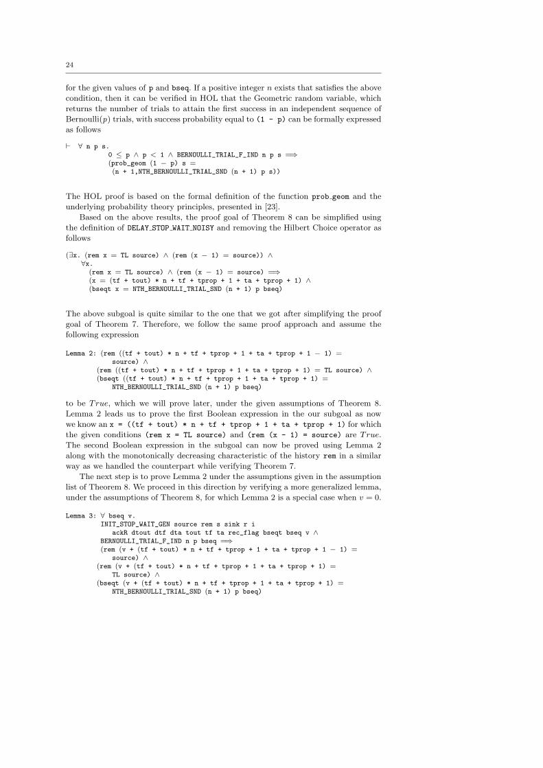
Based on the above results, the proof goal of Theorem 8 can be simplified using

the definition of DELAY STOP WAIT NOISY and removing the Hilbert Choice operator as

follows

(∃x. (rem x = TL source) ∧ (rem (x − 1) = source)) ∧∀x.

(rem x = TL source) ∧ (rem (x − 1) = source) =⇒(x = (tf + tout) * n + tf + tprop + 1 + ta + tprop + 1) ∧(bseqt x = NTH_BERNOULLI_TRIAL_SND (n + 1) p bseq)

The above subgoal is quite similar to the one that we got after simplifying the proof

goal of Theorem 7. Therefore, we follow the same proof approach and assume the

following expression

Lemma 2: (rem ((tf + tout) * n + tf + tprop + 1 + ta + tprop + 1 − 1) =source) ∧

(rem ((tf + tout) * n + tf + tprop + 1 + ta + tprop + 1) = TL source) ∧(bseqt ((tf + tout) * n + tf + tprop + 1 + ta + tprop + 1) =

NTH_BERNOULLI_TRIAL_SND (n + 1) p bseq)

to be True, which we will prove later, under the given assumptions of Theorem 8.

Lemma 2 leads us to prove the first Boolean expression in the our subgoal as now

we know an x = ((tf + tout) * n + tf + tprop + 1 + ta + tprop + 1) for which

the given conditions (rem x = TL source) and (rem (x - 1) = source) are True.

The second Boolean expression in the subgoal can now be proved using Lemma 2

along with the monotonically decreasing characteristic of the history rem in a similar

way as we handled the counterpart while verifying Theorem 7.

The next step is to prove Lemma 2 under the assumptions given in the assumption

list of Theorem 8. We proceed in this direction by verifying a more generalized lemma,

under the assumptions of Theorem 8, for which Lemma 2 is a special case when v = 0.

Lemma 3: ∀ bseq v.INIT_STOP_WAIT_GEN source rem s sink r i

ackR dtout dtf dta tout tf ta rec_flag bseqt bseq v ∧BERNOULLI_TRIAL_F_IND n p bseq =⇒(rem (v + (tf + tout) * n + tf + tprop + 1 + ta + tprop + 1 − 1) =

source) ∧(rem (v + (tf + tout) * n + tf + tprop + 1 + ta + tprop + 1) =

TL source) ∧(bseqt (v + (tf + tout) * n + tf + tprop + 1 + ta + tprop + 1) =

NTH_BERNOULLI_TRIAL_SND (n + 1) p bseq)

25

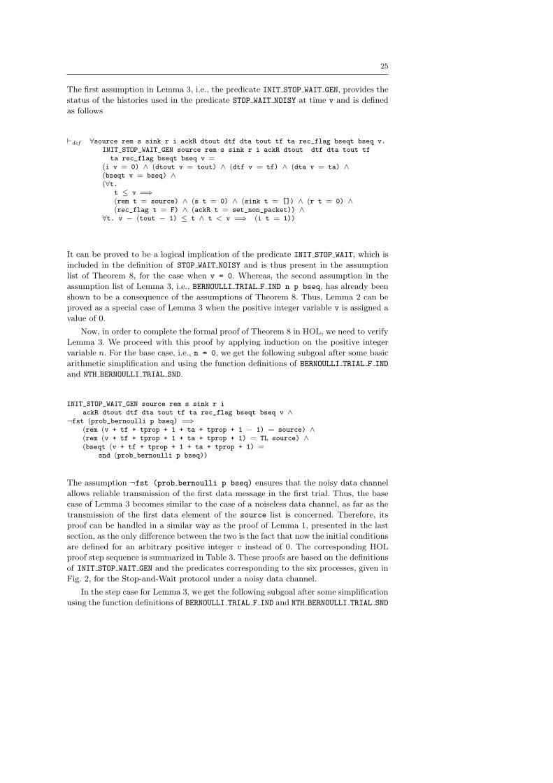
The first assumption in Lemma 3, i.e., the predicate INIT STOP WAIT GEN, provides the

status of the histories used in the predicate STOP WAIT NOISY at time v and is defined

as follows

`def ∀source rem s sink r i ackR dtout dtf dta tout tf ta rec_flag bseqt bseq v.INIT_STOP_WAIT_GEN source rem s sink r i ackR dtout dtf dta tout tfta rec_flag bseqt bseq v =

(i v = 0) ∧ (dtout v = tout) ∧ (dtf v = tf) ∧ (dta v = ta) ∧(bseqt v = bseq) ∧(∀t.

t ≤ v =⇒(rem t = source) ∧ (s t = 0) ∧ (sink t = []) ∧ (r t = 0) ∧(rec_flag t = F) ∧ (ackR t = set_non_packet)) ∧

∀t. v − (tout − 1) ≤ t ∧ t < v =⇒ (i t = 1))

It can be proved to be a logical implication of the predicate INIT STOP WAIT, which is

included in the definition of STOP WAIT NOISY and is thus present in the assumption

list of Theorem 8, for the case when v = 0. Whereas, the second assumption in the

assumption list of Lemma 3, i.e., BERNOULLI TRIAL F IND n p bseq, has already been

shown to be a consequence of the assumptions of Theorem 8. Thus, Lemma 2 can be

proved as a special case of Lemma 3 when the positive integer variable v is assigned a

value of 0.

Now, in order to complete the formal proof of Theorem 8 in HOL, we need to verify

Lemma 3. We proceed with this proof by applying induction on the positive integer

variable n. For the base case, i.e., n = 0, we get the following subgoal after some basic

arithmetic simplification and using the function definitions of BERNOULLI TRIAL F IND

and NTH BERNOULLI TRIAL SND.

INIT_STOP_WAIT_GEN source rem s sink r iackR dtout dtf dta tout tf ta rec_flag bseqt bseq v ∧

¬fst (prob_bernoulli p bseq) =⇒(rem (v + tf + tprop + 1 + ta + tprop + 1 − 1) = source) ∧(rem (v + tf + tprop + 1 + ta + tprop + 1) = TL source) ∧(bseqt (v + tf + tprop + 1 + ta + tprop + 1) =

snd (prob_bernoulli p bseq))

The assumption ¬fst (prob bernoulli p bseq) ensures that the noisy data channel

allows reliable transmission of the first data message in the first trial. Thus, the base

case of Lemma 3 becomes similar to the case of a noiseless data channel, as far as the

transmission of the first data element of the source list is concerned. Therefore, its

proof can be handled in a similar way as the proof of Lemma 1, presented in the last

section, as the only difference between the two is the fact that now the initial conditions

are defined for an arbitrary positive integer v instead of 0. The corresponding HOL

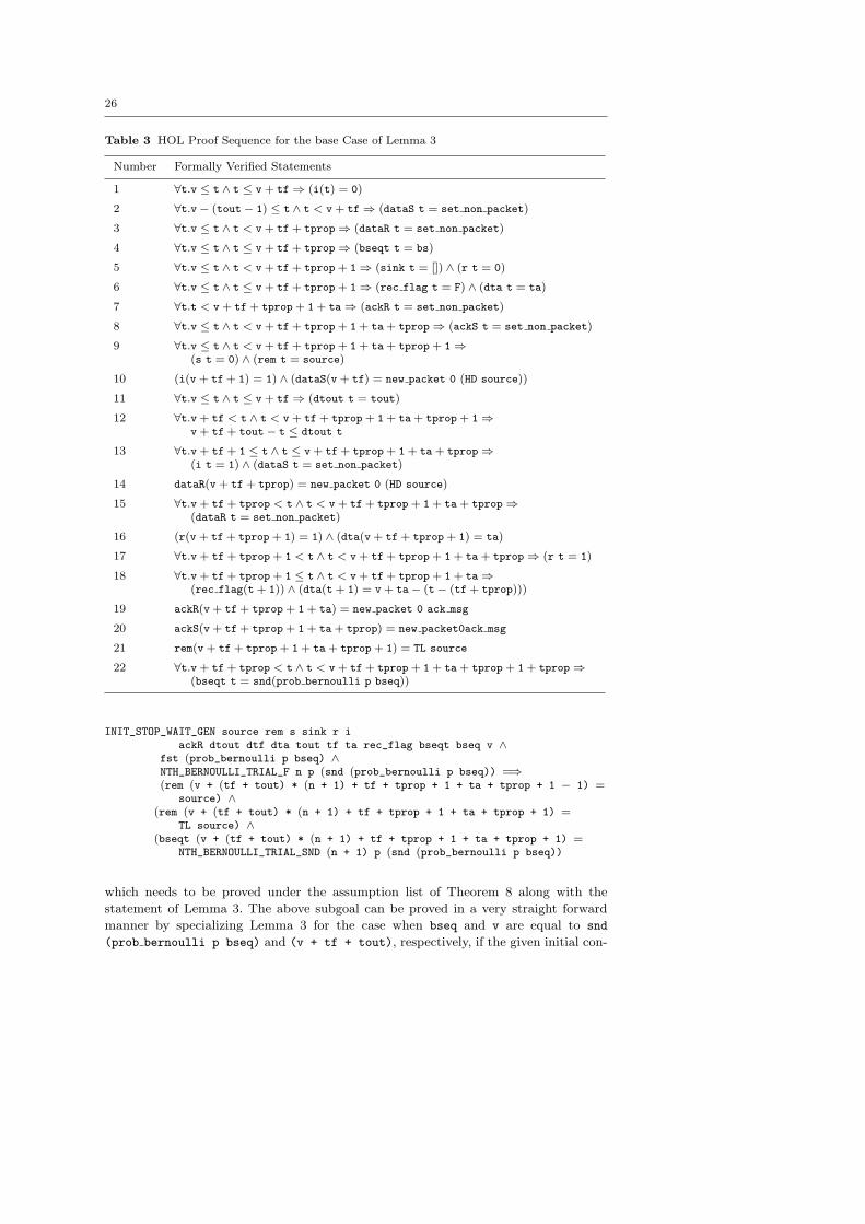
proof step sequence is summarized in Table 3. These proofs are based on the definitions

of INIT STOP WAIT GEN and the predicates corresponding to the six processes, given in

Fig. 2, for the Stop-and-Wait protocol under a noisy data channel.

In the step case for Lemma 3, we get the following subgoal after some simplification

using the function definitions of BERNOULLI TRIAL F IND and NTH BERNOULLI TRIAL SND

26

Table 3 HOL Proof Sequence for the base Case of Lemma 3

Number Formally Verified Statements

1 ∀t.v ≤ t ∧ t ≤ v + tf⇒ (i(t) = 0)

2 ∀t.v− (tout− 1) ≤ t ∧ t < v + tf⇒ (dataS t = set non packet)

3 ∀t.v ≤ t ∧ t < v + tf + tprop⇒ (dataR t = set non packet)

4 ∀t.v ≤ t ∧ t ≤ v + tf + tprop⇒ (bseqt t = bs)

5 ∀t.v ≤ t ∧ t < v + tf + tprop + 1⇒ (sink t = []) ∧ (r t = 0)

6 ∀t.v ≤ t ∧ t ≤ v + tf + tprop + 1⇒ (rec flag t = F) ∧ (dta t = ta)

7 ∀t.t < v + tf + tprop + 1 + ta⇒ (ackR t = set non packet)

8 ∀t.v ≤ t ∧ t < v + tf + tprop + 1 + ta + tprop⇒ (ackS t = set non packet)

9 ∀t.v ≤ t ∧ t < v + tf + tprop + 1 + ta + tprop + 1⇒(s t = 0) ∧ (rem t = source)

10 (i(v + tf + 1) = 1) ∧ (dataS(v + tf) = new packet 0 (HD source))

11 ∀t.v ≤ t ∧ t ≤ v + tf⇒ (dtout t = tout)

12 ∀t.v + tf < t ∧ t < v + tf + tprop + 1 + ta + tprop + 1⇒v + tf + tout− t ≤ dtout t

13 ∀t.v + tf + 1 ≤ t ∧ t ≤ v + tf + tprop + 1 + ta + tprop⇒(i t = 1) ∧ (dataS t = set non packet)

14 dataR(v + tf + tprop) = new packet 0 (HD source)

15 ∀t.v + tf + tprop < t ∧ t < v + tf + tprop + 1 + ta + tprop⇒(dataR t = set non packet)

16 (r(v + tf + tprop + 1) = 1) ∧ (dta(v + tf + tprop + 1) = ta)

17 ∀t.v + tf + tprop + 1 < t ∧ t < v + tf + tprop + 1 + ta + tprop⇒ (r t = 1)

18 ∀t.v + tf + tprop + 1 ≤ t ∧ t < v + tf + tprop + 1 + ta⇒(rec flag(t + 1)) ∧ (dta(t + 1) = v + ta− (t− (tf + tprop)))

19 ackR(v + tf + tprop + 1 + ta) = new packet 0 ack msg

20 ackS(v + tf + tprop + 1 + ta + tprop) = new packet0ack msg

21 rem(v + tf + tprop + 1 + ta + tprop + 1) = TL source

22 ∀t.v + tf + tprop < t ∧ t < v + tf + tprop + 1 + ta + tprop + 1 + tprop⇒(bseqt t = snd(prob bernoulli p bseq))

INIT_STOP_WAIT_GEN source rem s sink r iackR dtout dtf dta tout tf ta rec_flag bseqt bseq v ∧

fst (prob_bernoulli p bseq) ∧NTH_BERNOULLI_TRIAL_F n p (snd (prob_bernoulli p bseq)) =⇒(rem (v + (tf + tout) * (n + 1) + tf + tprop + 1 + ta + tprop + 1 − 1) =

source) ∧(rem (v + (tf + tout) * (n + 1) + tf + tprop + 1 + ta + tprop + 1) =

TL source) ∧(bseqt (v + (tf + tout) * (n + 1) + tf + tprop + 1 + ta + tprop + 1) =

NTH_BERNOULLI_TRIAL_SND (n + 1) p (snd (prob_bernoulli p bseq))

which needs to be proved under the assumption list of Theorem 8 along with the

statement of Lemma 3. The above subgoal can be proved in a very straight forward

manner by specializing Lemma 3 for the case when bseq and v are equal to snd

(prob bernoulli p bseq) and (v + tf + tout), respectively, if the given initial con-

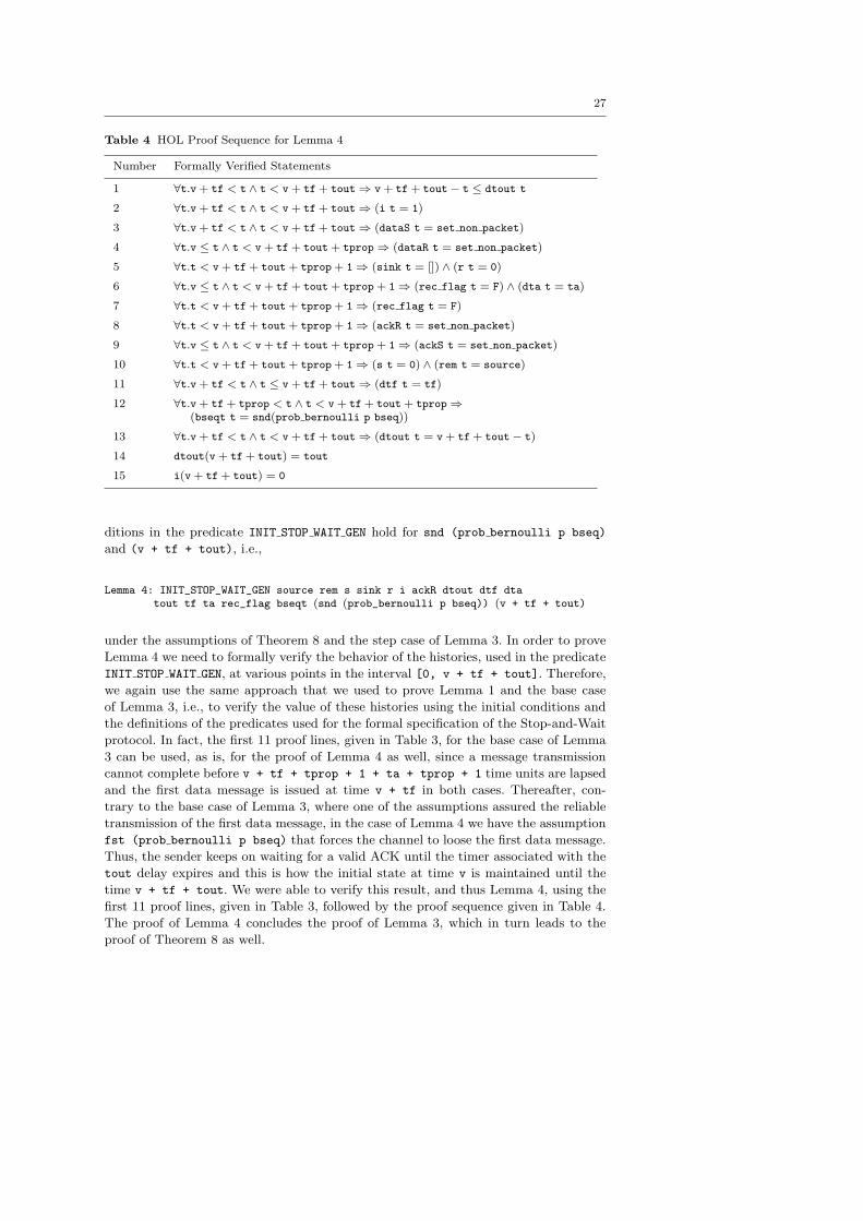
27

Table 4 HOL Proof Sequence for Lemma 4

Number Formally Verified Statements

1 ∀t.v + tf < t ∧ t < v + tf + tout⇒ v + tf + tout− t ≤ dtout t

2 ∀t.v + tf < t ∧ t < v + tf + tout⇒ (i t = 1)

3 ∀t.v + tf < t ∧ t < v + tf + tout⇒ (dataS t = set non packet)

4 ∀t.v ≤ t ∧ t < v + tf + tout + tprop⇒ (dataR t = set non packet)

5 ∀t.t < v + tf + tout + tprop + 1⇒ (sink t = []) ∧ (r t = 0)

6 ∀t.v ≤ t ∧ t < v + tf + tout + tprop + 1⇒ (rec flag t = F) ∧ (dta t = ta)

7 ∀t.t < v + tf + tout + tprop + 1⇒ (rec flag t = F)

8 ∀t.t < v + tf + tout + tprop + 1⇒ (ackR t = set non packet)

9 ∀t.v ≤ t ∧ t < v + tf + tout + tprop + 1⇒ (ackS t = set non packet)

10 ∀t.t < v + tf + tout + tprop + 1⇒ (s t = 0) ∧ (rem t = source)

11 ∀t.v + tf < t ∧ t ≤ v + tf + tout⇒ (dtf t = tf)

12 ∀t.v + tf + tprop < t ∧ t < v + tf + tout + tprop⇒(bseqt t = snd(prob bernoulli p bseq))

13 ∀t.v + tf < t ∧ t < v + tf + tout⇒ (dtout t = v + tf + tout− t)

14 dtout(v + tf + tout) = tout

15 i(v + tf + tout) = 0

ditions in the predicate INIT STOP WAIT GEN hold for snd (prob bernoulli p bseq)

and (v + tf + tout), i.e.,

Lemma 4: INIT_STOP_WAIT_GEN source rem s sink r i ackR dtout dtf dtatout tf ta rec_flag bseqt (snd (prob_bernoulli p bseq)) (v + tf + tout)

under the assumptions of Theorem 8 and the step case of Lemma 3. In order to prove

Lemma 4 we need to formally verify the behavior of the histories, used in the predicate

INIT STOP WAIT GEN, at various points in the interval [0, v + tf + tout]. Therefore,

we again use the same approach that we used to prove Lemma 1 and the base case

of Lemma 3, i.e., to verify the value of these histories using the initial conditions and

the definitions of the predicates used for the formal specification of the Stop-and-Wait

protocol. In fact, the first 11 proof lines, given in Table 3, for the base case of Lemma

3 can be used, as is, for the proof of Lemma 4 as well, since a message transmission

cannot complete before v + tf + tprop + 1 + ta + tprop + 1 time units are lapsed

and the first data message is issued at time v + tf in both cases. Thereafter, con-

trary to the base case of Lemma 3, where one of the assumptions assured the reliable

transmission of the first data message, in the case of Lemma 4 we have the assumption

fst (prob bernoulli p bseq) that forces the channel to loose the first data message.

Thus, the sender keeps on waiting for a valid ACK until the timer associated with the

tout delay expires and this is how the initial state at time v is maintained until the

time v + tf + tout. We were able to verify this result, and thus Lemma 4, using the

first 11 proof lines, given in Table 3, followed by the proof sequence given in Table 4.

The proof of Lemma 4 concludes the proof of Lemma 3, which in turn leads to the

proof of Theorem 8 as well.

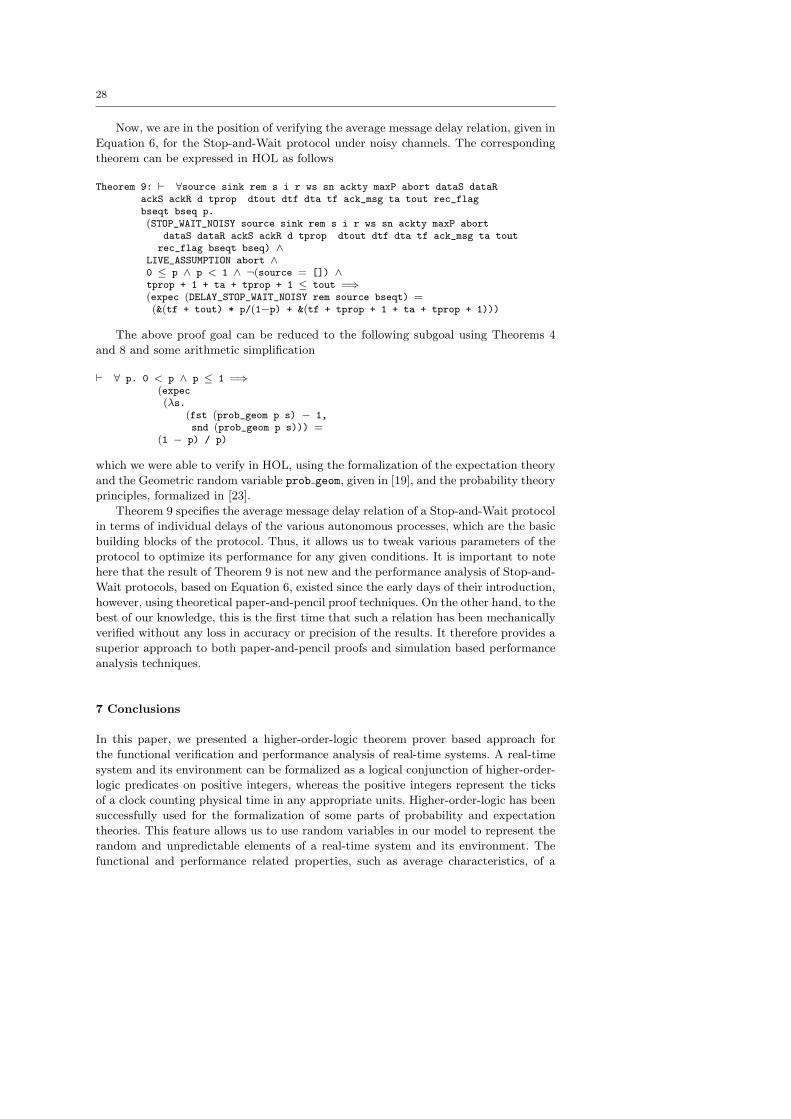
28

Now, we are in the position of verifying the average message delay relation, given in

Equation 6, for the Stop-and-Wait protocol under noisy channels. The corresponding

theorem can be expressed in HOL as follows

Theorem 9: ` ∀source sink rem s i r ws sn ackty maxP abort dataS dataRackS ackR d tprop dtout dtf dta tf ack_msg ta tout rec_flagbseqt bseq p.(STOP_WAIT_NOISY source sink rem s i r ws sn ackty maxP abort

dataS dataR ackS ackR d tprop dtout dtf dta tf ack_msg ta toutrec_flag bseqt bseq) ∧

LIVE_ASSUMPTION abort ∧0 ≤ p ∧ p < 1 ∧ ¬(source = []) ∧tprop + 1 + ta + tprop + 1 ≤ tout =⇒(expec (DELAY_STOP_WAIT_NOISY rem source bseqt) =(&(tf + tout) * p/(1−p) + &(tf + tprop + 1 + ta + tprop + 1)))

The above proof goal can be reduced to the following subgoal using Theorems 4

and 8 and some arithmetic simplification

` ∀ p. 0 < p ∧ p ≤ 1 =⇒(expec(λs.

(fst (prob_geom p s) − 1,snd (prob_geom p s))) =

(1 − p) / p)

which we were able to verify in HOL, using the formalization of the expectation theory

and the Geometric random variable prob geom, given in [19], and the probability theory

principles, formalized in [23].

Theorem 9 specifies the average message delay relation of a Stop-and-Wait protocol

in terms of individual delays of the various autonomous processes, which are the basic

building blocks of the protocol. Thus, it allows us to tweak various parameters of the

protocol to optimize its performance for any given conditions. It is important to note

here that the result of Theorem 9 is not new and the performance analysis of Stop-and-

Wait protocols, based on Equation 6, existed since the early days of their introduction,

however, using theoretical paper-and-pencil proof techniques. On the other hand, to the

best of our knowledge, this is the first time that such a relation has been mechanically

verified without any loss in accuracy or precision of the results. It therefore provides a

superior approach to both paper-and-pencil proofs and simulation based performance

analysis techniques.

7 Conclusions

In this paper, we presented a higher-order-logic theorem prover based approach for

the functional verification and performance analysis of real-time systems. A real-time

system and its environment can be formalized as a logical conjunction of higher-order-

logic predicates on positive integers, whereas the positive integers represent the ticks

of a clock counting physical time in any appropriate units. Higher-order-logic has been

successfully used for the formalization of some parts of probability and expectation

theories. This feature allows us to use random variables in our model to represent the

random and unpredictable elements of a real-time system and its environment. The

functional and performance related properties, such as average characteristics, of a

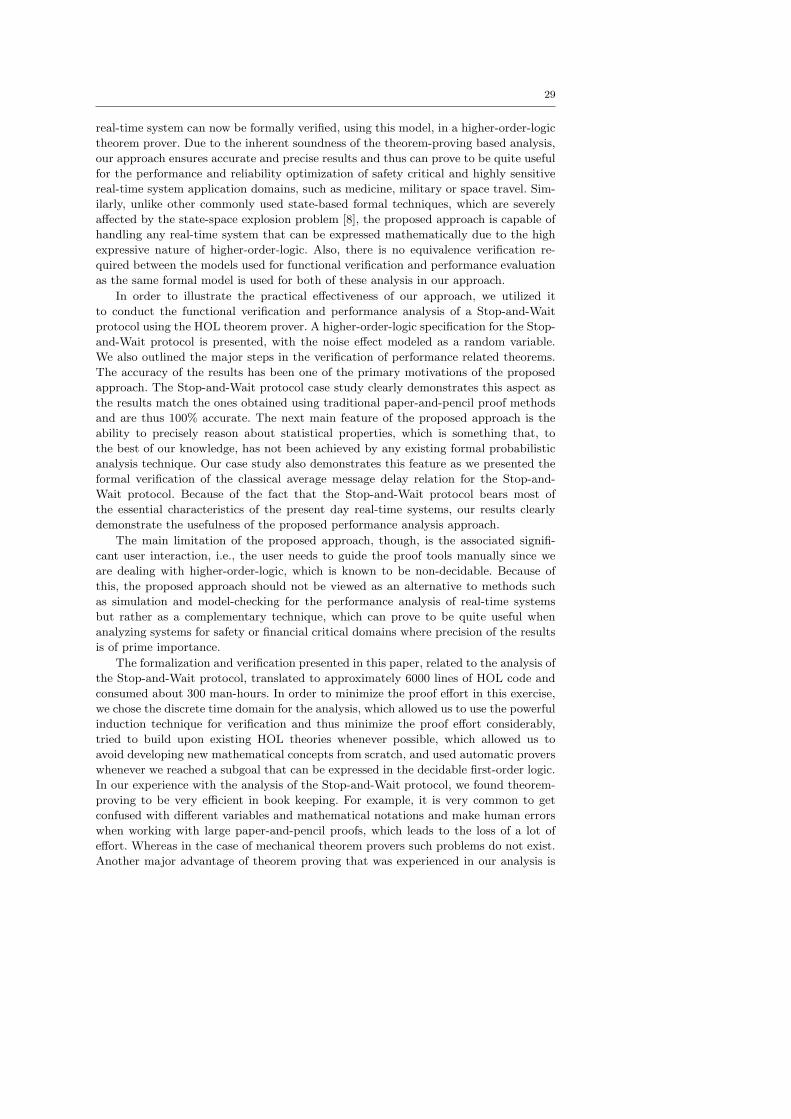
29

real-time system can now be formally verified, using this model, in a higher-order-logic

theorem prover. Due to the inherent soundness of the theorem-proving based analysis,

our approach ensures accurate and precise results and thus can prove to be quite useful

for the performance and reliability optimization of safety critical and highly sensitive

real-time system application domains, such as medicine, military or space travel. Sim-

ilarly, unlike other commonly used state-based formal techniques, which are severely

affected by the state-space explosion problem [8], the proposed approach is capable of

handling any real-time system that can be expressed mathematically due to the high

expressive nature of higher-order-logic. Also, there is no equivalence verification re-

quired between the models used for functional verification and performance evaluation

as the same formal model is used for both of these analysis in our approach.

In order to illustrate the practical effectiveness of our approach, we utilized it

to conduct the functional verification and performance analysis of a Stop-and-Wait

protocol using the HOL theorem prover. A higher-order-logic specification for the Stop-

and-Wait protocol is presented, with the noise effect modeled as a random variable.

We also outlined the major steps in the verification of performance related theorems.

The accuracy of the results has been one of the primary motivations of the proposed

approach. The Stop-and-Wait protocol case study clearly demonstrates this aspect as

the results match the ones obtained using traditional paper-and-pencil proof methods

and are thus 100% accurate. The next main feature of the proposed approach is the

ability to precisely reason about statistical properties, which is something that, to

the best of our knowledge, has not been achieved by any existing formal probabilistic

analysis technique. Our case study also demonstrates this feature as we presented the

formal verification of the classical average message delay relation for the Stop-and-

Wait protocol. Because of the fact that the Stop-and-Wait protocol bears most of

the essential characteristics of the present day real-time systems, our results clearly

demonstrate the usefulness of the proposed performance analysis approach.

The main limitation of the proposed approach, though, is the associated signifi-

cant user interaction, i.e., the user needs to guide the proof tools manually since we

are dealing with higher-order-logic, which is known to be non-decidable. Because of

this, the proposed approach should not be viewed as an alternative to methods such

as simulation and model-checking for the performance analysis of real-time systems

but rather as a complementary technique, which can prove to be quite useful when

analyzing systems for safety or financial critical domains where precision of the results

is of prime importance.

The formalization and verification presented in this paper, related to the analysis of

the Stop-and-Wait protocol, translated to approximately 6000 lines of HOL code and

consumed about 300 man-hours. In order to minimize the proof effort in this exercise,

we chose the discrete time domain for the analysis, which allowed us to use the powerful

induction technique for verification and thus minimize the proof effort considerably,

tried to build upon existing HOL theories whenever possible, which allowed us to

avoid developing new mathematical concepts from scratch, and used automatic provers

whenever we reached a subgoal that can be expressed in the decidable first-order logic.

In our experience with the analysis of the Stop-and-Wait protocol, we found theorem-

proving to be very efficient in book keeping. For example, it is very common to get

confused with different variables and mathematical notations and make human errors

when working with large paper-and-pencil proofs, which leads to the loss of a lot of

effort. Whereas in the case of mechanical theorem provers such problems do not exist.

Another major advantage of theorem proving that was experienced in our analysis is

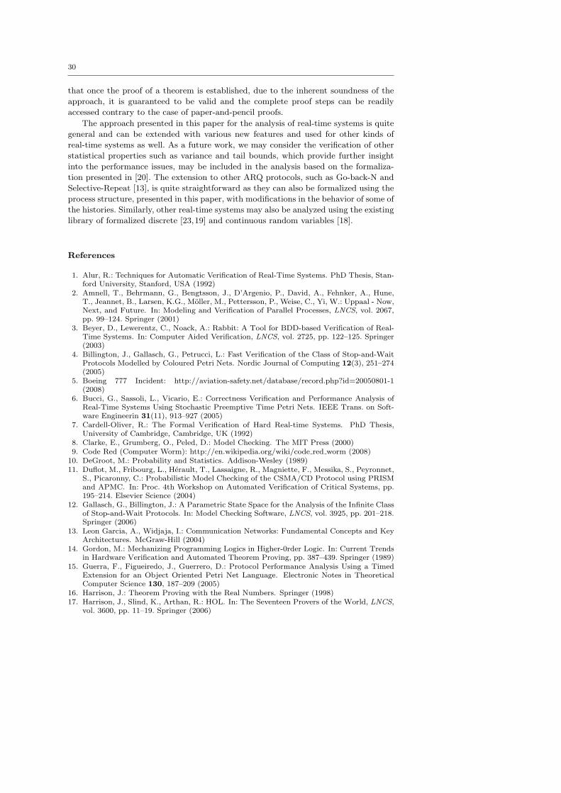
30

that once the proof of a theorem is established, due to the inherent soundness of the

approach, it is guaranteed to be valid and the complete proof steps can be readily

accessed contrary to the case of paper-and-pencil proofs.

The approach presented in this paper for the analysis of real-time systems is quite

general and can be extended with various new features and used for other kinds of

real-time systems as well. As a future work, we may consider the verification of other

statistical properties such as variance and tail bounds, which provide further insight

into the performance issues, may be included in the analysis based on the formaliza-

tion presented in [20]. The extension to other ARQ protocols, such as Go-back-N and

Selective-Repeat [13], is quite straightforward as they can also be formalized using the

process structure, presented in this paper, with modifications in the behavior of some of

the histories. Similarly, other real-time systems may also be analyzed using the existing

library of formalized discrete [23,19] and continuous random variables [18].

References

1. Alur, R.: Techniques for Automatic Verification of Real-Time Systems. PhD Thesis, Stan-ford University, Stanford, USA (1992)

2. Amnell, T., Behrmann, G., Bengtsson, J., D’Argenio, P., David, A., Fehnker, A., Hune,T., Jeannet, B., Larsen, K.G., Moller, M., Pettersson, P., Weise, C., Yi, W.: Uppaal - Now,Next, and Future. In: Modeling and Verification of Parallel Processes, LNCS, vol. 2067,pp. 99–124. Springer (2001)

3. Beyer, D., Lewerentz, C., Noack, A.: Rabbit: A Tool for BDD-based Verification of Real-Time Systems. In: Computer Aided Verification, LNCS, vol. 2725, pp. 122–125. Springer(2003)

4. Billington, J., Gallasch, G., Petrucci, L.: Fast Verification of the Class of Stop-and-WaitProtocols Modelled by Coloured Petri Nets. Nordic Journal of Computing 12(3), 251–274(2005)

5. Boeing 777 Incident: http://aviation-safety.net/database/record.php?id=20050801-1(2008)

6. Bucci, G., Sassoli, L., Vicario, E.: Correctness Verification and Performance Analysis ofReal-Time Systems Using Stochastic Preemptive Time Petri Nets. IEEE Trans. on Soft-ware Engineerin 31(11), 913–927 (2005)

7. Cardell-Oliver, R.: The Formal Verification of Hard Real-time Systems. PhD Thesis,University of Cambridge, Cambridge, UK (1992)

8. Clarke, E., Grumberg, O., Peled, D.: Model Checking. The MIT Press (2000)9. Code Red (Computer Worm): http://en.wikipedia.org/wiki/code red worm (2008)

10. DeGroot, M.: Probability and Statistics. Addison-Wesley (1989)11. Duflot, M., Fribourg, L., Herault, T., Lassaigne, R., Magniette, F., Messika, S., Peyronnet,

S., Picaronny, C.: Probabilistic Model Checking of the CSMA/CD Protocol using PRISMand APMC. In: Proc. 4th Workshop on Automated Verification of Critical Systems, pp.195–214. Elsevier Science (2004)

12. Gallasch, G., Billington, J.: A Parametric State Space for the Analysis of the Infinite Classof Stop-and-Wait Protocols. In: Model Checking Software, LNCS, vol. 3925, pp. 201–218.Springer (2006)

13. Leon Garcia, A., Widjaja, I.: Communication Networks: Fundamental Concepts and KeyArchitectures. McGraw-Hill (2004)

14. Gordon, M.: Mechanizing Programming Logics in Higher-0rder Logic. In: Current Trendsin Hardware Verification and Automated Theorem Proving, pp. 387–439. Springer (1989)

15. Guerra, F., Figueiredo, J., Guerrero, D.: Protocol Performance Analysis Using a TimedExtension for an Object Oriented Petri Net Language. Electronic Notes in TheoreticalComputer Science 130, 187–209 (2005)

16. Harrison, J.: Theorem Proving with the Real Numbers. Springer (1998)17. Harrison, J., Slind, K., Arthan, R.: HOL. In: The Seventeen Provers of the World, LNCS,

vol. 3600, pp. 11–19. Springer (2006)

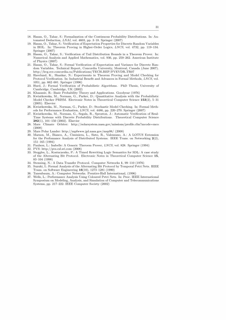
31

18. Hasan, O., Tahar, S.: Formalization of the Continuous Probability Distributions. In: Au-tomated Deduction, LNAI, vol. 4603, pp. 3–18. Springer (2007)

19. Hasan, O., Tahar, S.: Verification of Expectation Properties for Discrete Random Variablesin HOL. In: Theorem Proving in Higher-Order Logics, LNCS, vol. 4732, pp. 119–134.Springer (2007)

20. Hasan, O., Tahar, S.: Verification of Tail Distribution Bounds in a Theorem Prover. In:Numerical Analysis and Applied Mathematics, vol. 936, pp. 259–262. American Instituteof Physics (2007)

21. Hasan, O., Tahar, S.: Formal Verification of Expectation and Variance for Discrete Ran-dom Variables. Technical Report, Concordia University, Montreal, Canada (June 2007).http://hvg.ece.concordia.ca/Publications/TECH REP/FVEVDR TR07

22. Havelund, K., Shankar, N.: Experiments in Theorem Proving and Model Checking forProtocol Verification. In: Industrial Benefit and Advances in Formal Methods, LNCS, vol.1051, pp. 662–681. Springer (1996)

23. Hurd, J.: Formal Verification of Probabilistic Algorithms. PhD Thesis, University ofCambridge, Cambridge, UK (2002)

24. Khazanie, R.: Basic Probability Theory and Applications. Goodyear (1976)25. Kwiatkowska, M., Norman, G., Parker, D.: Quantitative Analysis with the Probabilistic

Model Checker PRISM. Electronic Notes in Theoretical Computer Science 153(2), 5–31(2005). Elsevier

26. Kwiatkowska, M., Norman, G., Parker, D.: Stochastic Model Checking. In: Formal Meth-ods for Performance Evaluation, LNCS, vol. 4486, pp. 220–270. Springer (2007)

27. Kwiatkowska, M., Norman, G., Segala, R., Sproston, J.: Automatic Verification of Real-Time Systems with Discrete Probability Distributions. Theoretical Computer Science282(1), 101–150 (2002). Elsevier

28. Mars Climate Orbiter: http://solarsystem.nasa.gov/missions/profile.cfm?mcode=mco(2008)

29. Mars Polar Lander: http://mpfwww.jpl.nasa.gov/msp98/ (2008)30. Marson, M., Bianco, A., Ciminiera, L., Sisto, R., Valenzano, A.: A LOTUS Extension

for the Perfomance Analysis of Distributed Systems. IEEE Trans. on Networking 2(2),151–165 (1994)

31. Paulson, L.: Isabelle: A Generic Theroem Prover, LNCS, vol. 828. Springer (1994)32. PVS: http://pvs.csl.sri.com (2008)33. Steggles, L., Kosiuczenko, P.: A Timed Rewriting Logic Semantics for SDL: A case study

of the Alternating Bit Protocol. Electronic Notes in Theoretical Computer Science 15,83–104 (1998)

34. Stenning, N.: A Data Transfer Protocol. Computer Networks 1, 99–110 (1976)35. Suzuki, I.: Formal Analysis of the Alternating Bit Protocol by Temporal Petri Nets. IEEE

Trans. on Software Engineering 16(10), 1273–1281 (1990)36. Tanenbaum, A.: Computer Networks. Prentice-Hall International, (1996)37. Wells, L.: Performance Analysis Using Coloured Petri Nets. In: Peoc. IEEE International

Symposium on Modeling, Analysis, and Simulation of Computer and TelecommunicationsSystems, pp. 217–222. IEEE Computer Society (2002)