Embed Size (px)
Citation preview
Working Paper/Document de travail 2013-43
Perceived Inflation Persistence
by Monica Jain
2
Bank of Canada Working Paper 2013-43
November 2013
Perceived Inflation Persistence
by
Monica Jain
Canadian Economic Analysis Department Bank of Canada
Ottawa, Ontario, Canada K1A 0G9 [email protected]
Bank of Canada working papers are theoretical or empirical works-in-progress on subjects in economics and finance. The views expressed in this paper are those of the author.
No responsibility for them should be attributed to the Bank of Canada.
ISSN 1701-9397 © 2013 Bank of Canada
ii
Acknowledgements
I am very thankful to Gregor Smith for his guidance, patience and supervision throughout this paper. I also thank Allan Gregory, Allen Head, Jonathan Wright, Nicolas Vincent, Rodrigo Sekkel, Norm Swanson, Brigitte Desroches, and participants at the CEA Conference (2010), the Midwest Macroeconomics Meetings (2011), the Bank of Canada Seminar Series (2011), the Atlanta Fed Seminar Series (2013) and the St. Louis Fed Applied Time Series Econometrics Workshop (2013) for helpful comments.
iii
Abstract
The Survey of Professional Forecasters (SPF) has had vast influence on research related to better understanding expectation formation and the behaviour of macroeconomic agents. Inflation expectations, in particular, have received a great deal of attention, since they play a crucial role in determining real interest rates, the expectations-augmented Phillips curve and monetary policy. One feature of the SPF that has surprisingly not been explored is the natural way in which it can be used to extract useful measures of inflation persistence. This paper presents a new measure of U.S. inflation persistence from the point of view of a professional forecaster, referred to as perceived inflation persistence. It is built via the implied autocorrelation function that follows from the estimates obtained using a forecaster-specific state-space model. Findings indicate that perceived inflation persistence has changed over time and that forecasters are more likely to view unexpected shocks to inflation as transitory, particularly since the mid-1990s. When compared to the autocorrelation function for actual inflation, forecasters react less to shocks than the actual inflation data would suggest, since they may engage in forecast smoothing.
JEL classification: E31, E37 Bank classification: Inflation and prices; Econometric and statistical methods
Résumé
L’enquête auprès des prévisionnistes professionnels a eu une influence considérable sur les recherches visant à acquérir une meilleure compréhension de la formation des anticipations et du comportement des agents macroéconomiques. Plus particulièrement, les attentes en matière d’inflation ont fait l’objet de nombreuses études, étant donné le rôle majeur qu’elles jouent dans la détermination des taux d’intérêt réels, de la courbe de Phillips dotée d’anticipations et de la politique monétaire. Étonnamment, un aspect qui n’a pas été exploré est la manière par laquelle cette enquête peut être utilisée pour extraire des mesures utiles de la persistance de l’inflation. L’auteure présente une nouvelle mesure de la persistance de l’inflation aux États-Unis telle qu’elle est perçue par les prévisionnistes professionnels. Cette mesure, qu’elle appelle persistance perçue de l’inflation, s’appuie sur la fonction d’autocorrélation implicite qui découle d’estimations obtenues à l’aide d’un modèle espace-état tenant compte de la spécificité de chaque prévisionniste. Les résultats indiquent que la persistance perçue de l’inflation a changé au fil du temps et que les prévisionnistes sont plus susceptibles de considérer les chocs d’inflation imprévus comme temporaires, particulièrement depuis le milieu des années 1990. La comparaison avec la fonction d’autocorrélation révèle que les prévisionnistes réagissent aux chocs dans une moindre mesure que ce que laissent entrevoir les données sur l’inflation réalisée, car ils lisseraient leurs prévisions.
Classification JEL : E31, E37 Classification de la Banque : Inflation et prix; Méthodes économétriques et statistiques
1 Introduction
Inflation persistence is a heavily debated property of inflation that can be defined as the
duration of shocks hitting inflation. At present, there is no consensus regarding the degree
or stability of inflation persistence: the empirical evidence differs across various measures of
inflation and time spans, as well as across different measures of persistence. An important
consequence of high inflation persistence is that it can undermine people’s confidence in the
central bank’s policies. Consequently, it may cause inflation expectations to differ from the
central bank’s objectives as inflation expectations become sensitive to shocks that hit the
economy. This may influence the level of actual inflation, despite the central bank’s policies
targeted at controlling it. For example, consider a substantial increase in the price of gasoline.
If the public viewed the central bank’s mandate to maintain price stability as credible, then
they would view the resulting increase in inflation as temporary and their expectations of
future inflation would be in line with the central bank’s objectives. Conversely, if the public
did not view the central bank as credible in maintaining price stability, persistently high
inflation could result, since the public would expect higher inflation in the future, and so
make price and wage decisions accordingly. In this case, the central bank may be required
to take a more aggressive response following an inflationary shock than would otherwise
be necessary, solely to achieve credibility with the public. Thus, persistence in expected
inflation may raise the output costs associated with stabilizing actual inflation, and without
a concrete consensus regarding inflation persistence, it is diffi cult to determine the extent of
these costs.
This paper takes a different approach to tackle this challenge by introducing a novel
measure, called perceived inflation persistence, to extract persistence estimates from inflation-
expectations data. Perceived inflation persistence measures the persistence of inflation from
the point of view of a forecaster. Obtaining this measure is not a straightforward task, since
people are not asked to quantify or report their views on inflation persistence. Moreover,
agents are heterogeneous in the way in which they form inflation expectations, making it
2
diffi cult to deduce their implied persistence. One reason for this heterogeneity is that agents
may have different loss functions. Alternatively, agents may have heterogeneous information
sets, so the differences in their expectations reflect this different information.
The methodology developed in this paper to identify perceived inflation persistence can
be applied to many related issues, such as understanding forecasters’views on the persistence
of shocks to different macroeconomic variables. In addition, recognizing that forecasters are
heterogeneous, they are not assumed to have identical information sets: differences in their
perceptions are allowed for, making it possible to generate a distribution of implied estimates
of persistence that can be tested for stability across forecasters.
The method used to identify perceptions of inflation persistence in this paper does not
presume a particular model, but, in the context of a state-space model, provides a useful
means of comparison between the measure introduced in this paper and other measures of
inflation persistence. In a state-space model, inflation comprises a persistent, forecaster-
specific state variable that evolves according to an AR(1) process, plus a transitory noise
component. State persistence is measured as the autocorrelation in the state variable and is
shown to be closely related to inflation predictability, which has been equated with inflation
persistence in recent literature. Furthermore, once an estimate of state persistence is obtained
for each forecaster, it can be used to compute forecasters’implied autocorrelation functions,
giving an estimate of perceived inflation persistence that may be directly compared to actual
inflation persistence. The results suggest that, likely due to forecast smoothing by forecasters,
their forecasts react less to shocks than actual inflation data would suggest.
This paper is organized as follows. Section 2 reviews the literature related to the study
of inflation persistence and the use of data obtained from surveys of professional forecasters.
Section 3 discusses the relationship between forecast revisions and persistence, and the state-
space model. Section 4 describes the data used and section 5 reports the estimation results.
Section 6 concludes.
3
2 Research Context
2.1 U.S. inflation persistence
Much research has been dedicated to determining the degree of inflation persistence along
with its stability over time. Cogley and Sargent (2001) use a vector autoregression (VAR)
with random coeffi cients to measure parameter drift in U.S. inflation-unemployment-interest
rate dynamics. They find that, since the early 1980s, the degree of persistence in CPI
inflation has been drifting downwards. This result coincides with the findings of Taylor
(2000), who uses the GDP deflator, and Brainard and Perry (2000), who use the CPI.
Similar to Cogley and Sargent (2001), Pivetta and Reis (2007) use Bayesian methods
to estimate inflation dynamics using the GDP deflator, but allow for the possibility that
inflation may have a unit root. They compute alternative statistical measures of inflation
persistence and, as a result, find that inflation persistence in the United States has been
unchanged over the past three decades and that the data cannot reject the possibility of a
unit root. Sims (2001) and Stock (2001) also maintain that inflation persistence has been
unchanged over this time period using the CPI and GDP deflator, respectively.
Levin and Piger (2004) apply both classical and Bayesian econometric methods to char-
acterize the dynamic behaviour of inflation from 1984 to 2003. They consider four different
measures of inflation: GDP price inflation, CPI inflation, core CPI inflation and personal
consumption expenditure (PCE) price inflation. Contrary to the findings by Pivetta and
Reis (2007), they find that once the model allows for structural breaks in the intercept (par-
ticularly in 1991 for the United States), all measures of inflation exhibit little persistence
over the sample period.
A possible source of disagreement stems from the fact that the literature focuses on
diverse features of inflation. In more recent work, Cogley, Primiceri and Sargent (2010)
study inflation-gap persistence in the United States using two measures of inflation: the log-
differences of the GDP and PCE chain-weighted price indices, measuring persistence in terms
4
of short- to medium-term predictability. They argue that the inflation gap, defined as the
difference between inflation and the Federal Reserve’s long-run inflation target, has become
less persistent since the Volcker disinflation, due to both monetary policy and non-policy
factors.
In the inflation-forecasting literature, Stock and Watson (2007) examine the extent
to which changes in the inflation process have made U.S. GDP inflation more diffi cult to
forecast. Using an unobserved component trend-cycle model with stochastic volatility, their
findings suggest that there have been major changes to the univariate inflation process that
has made inflation less persistent and volatile since 1984. Post-1984 inflation forecasting
models have smaller root-mean-squared errors (RMSE) than prior to 1984, suggesting that
inflation has become easier to forecast. At the same time, post-1984, it has become diffi cult
to improve on forecasts made beyond simple univariate models, making the job of an inflation
forecaster more diffi cult.
For the most part, there is agreement that inflation persistence was high from the 1960s
until the disinflationary period in the early 1980s. The controversy occurs in the subsequent
period from the early 1980s onwards; some researchers suggest that inflation persistence has
declined, while others contend that it has been unchanged. For example, Pivetta and Reis
(2007) find that postwar U.S. inflation persistence is always close to 1, with no evidence of a
decrease in recent years. They use multiple measures of inflation persistence to obtain this
result, including the largest autoregressive root and the sum of the autoregressive coeffi cients,
when inflation follows an AR(3) process. Conversely, Levin and Piger (2004) find that, since
1984, estimates of U.S. inflation persistence are less than 0.7 and the null hypothesis of a
unit root can be rejected at the 95% confidence level. Levin and Piger measure the degree
of inflation persistence in terms of the sum of the autoregressive coeffi cients when inflation
follows an AR(4) process.
In a related context, the literature on inflation persistence for an inflation-targeting
country such as Canada indicates that the persistence of both core and headline CPI inflation
5
has shown signs of significant decline since the 1980s. In fact, Mendes and Murchison (2009—
2010) find that the adoption of an explicit inflation target has likely played a key role in
this decline. Benati (2008) documents a similar decline in inflation persistence for Canada
as well as other countries that have adopted inflation-targeting regimes.
2.2 Forecast survey data
Many researchers have found that data obtained from surveys of professional forecasters
outperform simple time-series benchmarks in forecasting inflation: see Grant and Thomas
(1999), Thomas (1999), and Mehra (2002). Faust and Wright (2012) compare several meth-
ods of forecasting inflation and find that private sector survey forecasts are quite diffi cult
to beat. In addition, Ang, Bekaert and Wei (2007) examine the forecasting power of four
alternative methods of forecasting U.S. inflation out-of-sample: autoregressive integrated
moving-average (ARIMA) models, forecasts from a Phillips curve, term-structure models
and survey-based measures. They find that the Livingston Survey and the Survey of Profes-
sional Forecasters (SPF) outperform the other forecasting methods. Capistran and Timmer-
mann (2009) use data from the SPF to explain the dispersion in inflation expectations across
forecasters. Their paper is relevant because it highlights aspects of forecaster heterogeneity,
suggesting that the differences in beliefs are correlated with both the level and volatility of
inflation based on asymmetries in costs of over- and underpredicting inflation. Similarly,
Patton and Timmermann (2010) find that differences in agents’ forecasts of inflation are
greater at longer forecast horizons and that these differences persist over time.
Models in which agents are inattentive to new information have been proposed to ex-
plain heterogeneity in forecasts. Mankiw, Reis and Wolfers (2003), for example, document
disagreement in inflation expectations among both consumers and professional economists.
They suggest that this disagreement can provide insight into macroeconomic dynamics.
Their paper accounts for this heterogeneity by using a sticky-information model which sug-
gests that agents update their expectations only periodically, and therefore some agents may
6
form expectations based on outdated information. They find that the sticky-information
model is able to explain some (but not all) features of the data. Other forms of agent inat-
tention include noisy information models proposed by Woodford (2002), Sims (2003), and
Mackowiak and Wiederholt (2009), in which agents continuously update their information
but do not have perfect access to it. Andrade and Le Bihan (2010) estimate a model in
which forecasters have both sticky information and noisy information. Their work is one of
the few to highlight and exploit the panel dimension of a survey of professional forecasters,
in particular, the European Central Bank’s SPF.
This paper uses data from the U.S. SPF to measure perceived inflation persistence.
In light of the debate surrounding actual U.S. inflation persistence, I explore the panel
dimension of the SPF, enabling a comparison of estimates across forecasters.
3 Forecast Revisions and Persistence
3.1 Notation and test equation
The notation used to represent a forecast is Ejtπ(t+h), which is the inflation forecast made
by forecaster j, conditional on his or her time t information set, h-steps ahead. Forecasts are
typically made at the beginning of time t + 1, so the most recent period of information the
forecaster would have available would be time t. For example, Ejtπ(t + 1) and Ejtπ(t + 2)
would be the one-step-ahead and two-step-ahead inflation forecasts that forecaster j makes
based on time t information, respectively.
An h-step-ahead forecast revision is defined as
rπ(j, t, h) = Ejtπ(t+ h)− Ejt−1π(t+ h), h = 1, ..., H and J = 1, ..., J, (1)
where the revision is made with time t information. Notice that Ejtπ(t+h) and Ejt−1π(t+h)
are both forecasts of the same thing, π(t+h). However, revisions can be made to this forecast
7
from one period to the next as forecaster j’s information set changes.
In this paper, the central idea is that if forecasters believe that an inflationary shock
would have only temporary effects, they would not make substantial revisions to multiple
future inflation forecasts, and their perception of shock persistence would be low. On the
other hand, if forecasters believe that the central bank may not be able to maintain low and
stable inflation following a shock, they would make revisions to their inflation forecasts for
multiple future periods, and thus perceive the shock as being more persistent. Therefore,
the coeffi cient linking revisions made to inflation forecasts between multiple horizons can be
used to back out forecasters’views on inflationary shock persistence. Specifically, we will see
that, using the chain rule of forecasting, we can determine the relationship between revisions
at horizons h and h+ 1 as follows:
rπ(j, t, h+ 1) = a(j)rπ(j, t, h) h = 1, ..., H. (2)
Thus a(j)measures the state persistence for forecaster j, which we will see later is very closely
linked to forecaster j’s perceptions of inflation persistence.
3.2 State-space model
The state-space model described in this section is one example of a model that can help
identify perceptions of inflation persistence; there may be other suitable models that are
useful in this regard. The advantage here is that the model will provide a means to identify
perceptions with minimal assumptions on the models used by forecasters. This measure is
comparable to another measure of persistence used in the literature, namely, predictability,
which is discussed in more detail later in this section and in Appendix C.
To represent forecasts, I attribute to each forecaster j a state-space time-series model
8
for inflation:
π(t) = x(j, t) + ε(j, t) (3)
x(j, t) = a(j)x(j, t− 1) + η(j, t), (4)
where ε(j, t) and η(j, t) are serially uncorrelated error terms with ε(j, t) ∼ (0, σ2ε(j)) and
η(j, t) ∼ (0, σ2η(j)).1 One interpretation of this model is that forecaster j decomposes infla-
tion into persistent and transitory components, where ε(j, t) and η(j, t) are transitory and
persistent shocks to inflation, respectively. As pointed out by Gourinchas and Tornell (2004),
these shocks may capture agents’uncertainty regarding the conduct of monetary policy since
the central bank’s inflation target and information set are imperfectly known to forecasters.
The state variable x(j, t) can be interpreted as a scalar index of the variables that
forecaster j uses when calculating inflation expectations. The heterogeneity in this model
arises through x(j, t), which varies across forecasters and is unobserved (except to forecaster
j). I do not place any assumptions on the identity of x(j, t); I require only that it evolve
according to (4). First, x(j, t) may, for example, be π(t) itself. In this case, the state-space
model would become an AR(1) representation for inflation, allowing forecasters to have their
own views of inflation persistence. This framework includes several interesting special cases
and is explored further in Jain (2010). However, my more general state-space representation
allows for heterogeneity in both information sets and in state persistence.
Second, x(j, t) may be core inflation, the persistent part of inflation. Core inflation is
often used to forecast the CPI inflation rate (i.e., headline inflation). Since core inflation
excludes the most volatile components of headline inflation, it is a smoother series that can
better capture the trend in headline inflation. Hence, one can think of actual inflation as
being core inflation plus noise, as in (3).
1The set-up here is a forecaster-specific, stationary version of the unobserved component model in Stockand Watson (2007), without a drift. It is useful to note that the inclusion of a forecaster-specific constantterm in the state variable in (4) does not alter the calculation of state persistence. In both cases, theconstants cancel out during the calculation.
9
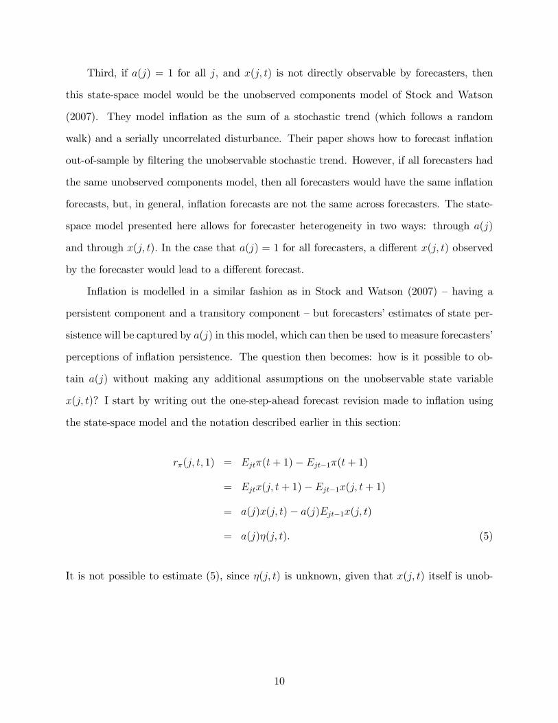
Third, if a(j) = 1 for all j, and x(j, t) is not directly observable by forecasters, then
this state-space model would be the unobserved components model of Stock and Watson
(2007). They model inflation as the sum of a stochastic trend (which follows a random
walk) and a serially uncorrelated disturbance. Their paper shows how to forecast inflation
out-of-sample by filtering the unobservable stochastic trend. However, if all forecasters had
the same unobserved components model, then all forecasters would have the same inflation
forecasts, but, in general, inflation forecasts are not the same across forecasters. The state-
space model presented here allows for forecaster heterogeneity in two ways: through a(j)
and through x(j, t). In the case that a(j) = 1 for all forecasters, a different x(j, t) observed
by the forecaster would lead to a different forecast.
Inflation is modelled in a similar fashion as in Stock and Watson (2007) —having a
persistent component and a transitory component —but forecasters’estimates of state per-
sistence will be captured by a(j) in this model, which can then be used to measure forecasters’
perceptions of inflation persistence. The question then becomes: how is it possible to ob-
tain a(j) without making any additional assumptions on the unobservable state variable
x(j, t)? I start by writing out the one-step-ahead forecast revision made to inflation using
the state-space model and the notation described earlier in this section:
rπ(j, t, 1) = Ejtπ(t+ 1)− Ejt−1π(t+ 1)
= Ejtx(j, t+ 1)− Ejt−1x(j, t+ 1)
= a(j)x(j, t)− a(j)Ejt−1x(j, t)
= a(j)η(j, t). (5)
It is not possible to estimate (5), since η(j, t) is unknown, given that x(j, t) itself is unob-
10
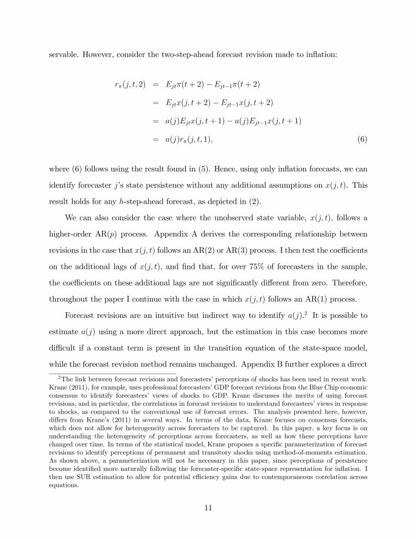
servable. However, consider the two-step-ahead forecast revision made to inflation:
rπ(j, t, 2) = Ejtπ(t+ 2)− Ejt−1π(t+ 2)
= Ejtx(j, t+ 2)− Ejt−1x(j, t+ 2)
= a(j)Ejtx(j, t+ 1)− a(j)Ejt−1x(j, t+ 1)
= a(j)rπ(j, t, 1), (6)
where (6) follows using the result found in (5). Hence, using only inflation forecasts, we can
identify forecaster j’s state persistence without any additional assumptions on x(j, t). This
result holds for any h-step-ahead forecast, as depicted in (2).
We can also consider the case where the unobserved state variable, x(j, t), follows a
higher-order AR(p) process. Appendix A derives the corresponding relationship between
revisions in the case that x(j, t) follows an AR(2) or AR(3) process. I then test the coeffi cients
on the additional lags of x(j, t), and find that, for over 75% of forecasters in the sample,
the coeffi cients on these additional lags are not significantly different from zero. Therefore,
throughout the paper I continue with the case in which x(j, t) follows an AR(1) process.
Forecast revisions are an intuitive but indirect way to identify a(j).2 It is possible to
estimate a(j) using a more direct approach, but the estimation in this case becomes more
diffi cult if a constant term is present in the transition equation of the state-space model,
while the forecast revision method remains unchanged. Appendix B further explores a direct
2The link between forecast revisions and forecasters’perceptions of shocks has been used in recent work.Krane (2011), for example, uses professional forecasters’GDP forecast revisions from the Blue Chip economicconsensus to identify forecasters’ views of shocks to GDP. Krane discusses the merits of using forecastrevisions, and in particular, the correlations in forecast revisions to understand forecasters’views in responseto shocks, as compared to the conventional use of forecast errors. The analysis presented here, however,differs from Krane’s (2011) in several ways. In terms of the data, Krane focuses on consensus forecasts,which does not allow for heterogeneity across forecasters to be captured. In this paper, a key focus is onunderstanding the heterogeneity of perceptions across forecasters, as well as how these perceptions havechanged over time. In terms of the statistical model, Krane proposes a specific parameterization of forecastrevisions to identify perceptions of permanent and transitory shocks using method-of-moments estimation.As shown above, a parameterization will not be necessary in this paper, since perceptions of persistencebecome identified more naturally following the forecaster-specific state-space representation for inflation. Ithen use SUR estimation to allow for potential effi ciency gains due to contemporaneous correlation acrossequations.
11
method of estimating a(j) in this case.
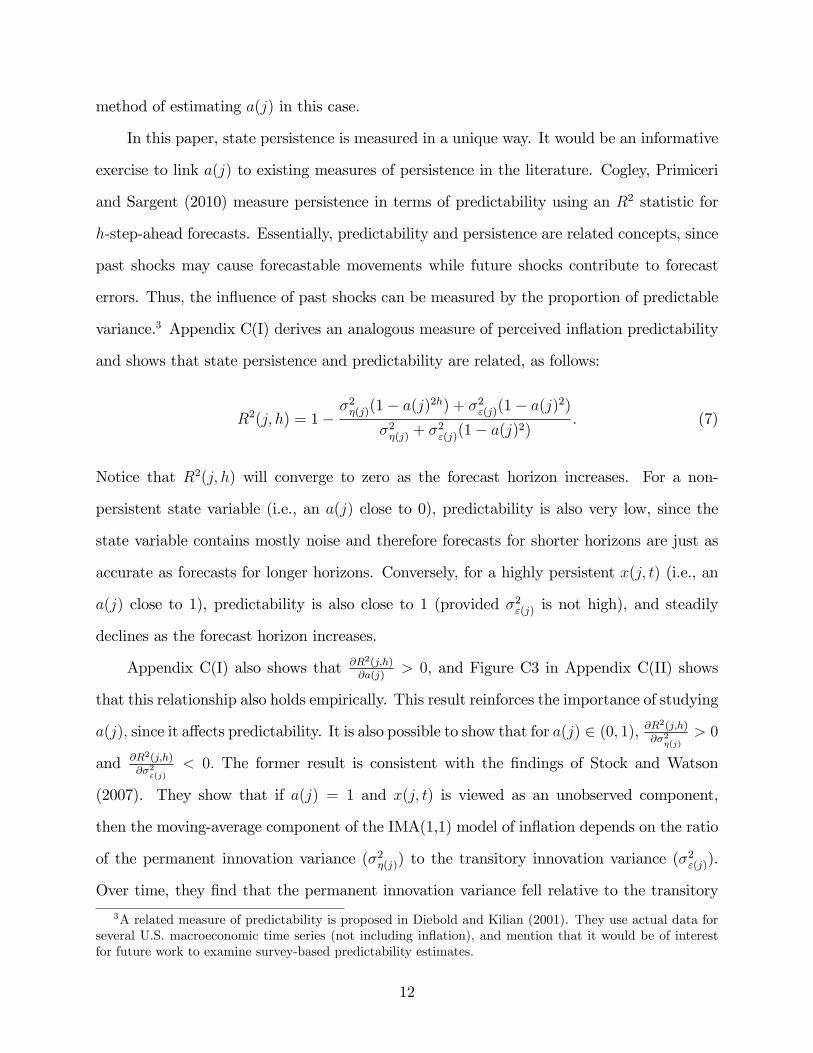
In this paper, state persistence is measured in a unique way. It would be an informative
exercise to link a(j) to existing measures of persistence in the literature. Cogley, Primiceri
and Sargent (2010) measure persistence in terms of predictability using an R2 statistic for
h-step-ahead forecasts. Essentially, predictability and persistence are related concepts, since
past shocks may cause forecastable movements while future shocks contribute to forecast
errors. Thus, the influence of past shocks can be measured by the proportion of predictable
variance.3 Appendix C(I) derives an analogous measure of perceived inflation predictability
and shows that state persistence and predictability are related, as follows:
R2(j, h) = 1−σ2η(j)(1− a(j)2h) + σ2ε(j)(1− a(j)2)
σ2η(j) + σ2ε(j)(1− a(j)2). (7)
Notice that R2(j, h) will converge to zero as the forecast horizon increases. For a non-
persistent state variable (i.e., an a(j) close to 0), predictability is also very low, since the
state variable contains mostly noise and therefore forecasts for shorter horizons are just as
accurate as forecasts for longer horizons. Conversely, for a highly persistent x(j, t) (i.e., an
a(j) close to 1), predictability is also close to 1 (provided σ2ε(j) is not high), and steadily
declines as the forecast horizon increases.
Appendix C(I) also shows that ∂R2(j,h)∂a(j)
> 0, and Figure C3 in Appendix C(II) shows
that this relationship also holds empirically. This result reinforces the importance of studying
a(j), since it affects predictability. It is also possible to show that for a(j) ∈ (0, 1), ∂R2(j,h)
∂σ2η(j)
> 0
and ∂R2(j,h)
∂σ2ε(j)
< 0. The former result is consistent with the findings of Stock and Watson
(2007). They show that if a(j) = 1 and x(j, t) is viewed as an unobserved component,
then the moving-average component of the IMA(1,1) model of inflation depends on the ratio
of the permanent innovation variance (σ2η(j)) to the transitory innovation variance (σ2ε(j)).
Over time, they find that the permanent innovation variance fell relative to the transitory
3A related measure of predictability is proposed in Diebold and Kilian (2001). They use actual data forseveral U.S. macroeconomic time series (not including inflation), and mention that it would be of interestfor future work to examine survey-based predictability estimates.
12
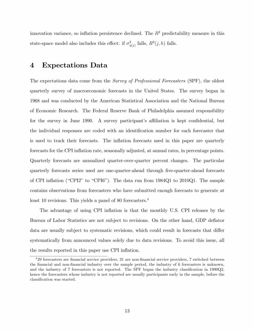
innovation variance, so inflation persistence declined. The R2 predictability measure in this
state-space model also includes this effect: if σ2η(j) falls, R2(j, h) falls.
4 Expectations Data
The expectations data come from the Survey of Professional Forecasters (SPF), the oldest
quarterly survey of macroeconomic forecasts in the United States. The survey began in
1968 and was conducted by the American Statistical Association and the National Bureau
of Economic Research. The Federal Reserve Bank of Philadelphia assumed responsibility
for the survey in June 1990. A survey participant’s affi liation is kept confidential, but
the individual responses are coded with an identification number for each forecaster that
is used to track their forecasts. The inflation forecasts used in this paper are quarterly
forecasts for the CPI inflation rate, seasonally adjusted, at annual rates, in percentage points.
Quarterly forecasts are annualized quarter-over-quarter percent changes. The particular
quarterly forecasts series used are one-quarter-ahead through five-quarter-ahead forecasts
of CPI inflation (“CPI2”to “CPI6”). The data run from 1984Q1 to 2010Q1. The sample
contains observations from forecasters who have submitted enough forecasts to generate at
least 10 revisions. This yields a panel of 80 forecasters.4
The advantage of using CPI inflation is that the monthly U.S. CPI releases by the
Bureau of Labor Statistics are not subject to revisions. On the other hand, GDP deflator
data are usually subject to systematic revisions, which could result in forecasts that differ
systematically from announced values solely due to data revisions. To avoid this issue, all
the results reported in this paper use CPI inflation.
429 forecasters are financial service providers, 31 are non-financial service providers, 7 switched betweenthe financial and non-financial industry over the sample period, the industry of 6 forecasters is unknown,and the industry of 7 forecasters is not reported. The SPF began the industry classification in 1990Q2,hence the forecasters whose industry is not reported are usually participants early in the sample, before theclassification was started.
13
5 Estimation Results
5.1 Seemingly unrelated regression (SUR) estimation
For each forecaster j, a(j) can be interpreted as the slope of equation (2). I proceed by
estimating the following equations jointly using SUR estimation:
rπ(j, t, 2) = υ(j, 2) + a(j)rπ(j, t, 1) + ν(j, t, 2) (8)
rπ(j, t, 3) = υ(j, 3) + a(j)rπ(j, t, 2) + ν(j, t, 3) (9)
rπ(j, t, 4) = υ(j, 4) + a(j)rπ(j, t, 3) + ν(j, t, 4), (10)
where υ is the intercept and ν is the error term.5 The set-up follows, since the SPF provides
forecasts up to five quarters ahead, allowing state persistence to be estimated using three
equations.6 ,7 Estimating these equations jointly using a SUR estimator enables me to impose
cross-equation restrictions.8
Ideally, estimation would be performed with a panel of fixed composition, with most
forecasters participating and relatively few missing observations. But since many observa-
tions are missing, it is not possible to find overlapping time periods for a large number
of forecasters. In addition, calculating a forecast revision requires at least two consecutive
forecasts. I proceed to the estimation keeping in mind this limitation of the data set.
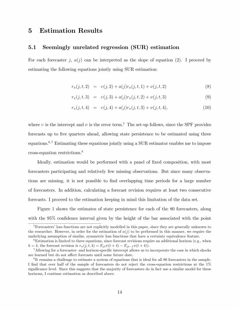
Figure 1 shows the estimates of state persistence for each of the 80 forecasters, along
with the 95% confidence interval given by the height of the bar associated with the point
5Forecasters’loss functions are not explicitly modelled in this paper, since they are generally unknown tothe researcher. However, in order for the estimation of a(j) to be performed in this manner, we require theunderlying assumption of similar, symmetric loss functions that have a certainty equivalence feature.
6Estimation is limited to three equations, since forecast revisions require an additional horizon (e.g., whenh = 4, the forecast revision is rπ(j, t, 4) = Ejtπ(t+ 4)− Ejt−1π(t+ 4)).
7Allowing for a forecaster- and horizon-specific intercept allows us to incorporate the case in which shocksare learned but do not affect forecasts until some future date.
8It remains a challenge to estimate a system of equations that is ideal for all 80 forecasters in the sample.I find that over half of the sample of forecasters do not reject the cross-equation restrictions at the 1%significance level. Since this suggests that the majority of forecasters do in fact use a similar model for thesehorizons, I continue estimation as described above.
14
estimate. Notice that, first, very few forecasters have point estimates near 1, which would
indicate a unit root in state persistence. Second, of the 80 forecasters, 13 have estimates
that are not statistically different from zero at the 5% significance level; the majority of
these forecasters can be seen in Figure 1 as having slightly negative estimates of a(j) or
estimates of a(j) very close to zero. Third, there is substantial variation in the precision
of the estimates across forecasters; some of this is due to the inclusion of forecasters with
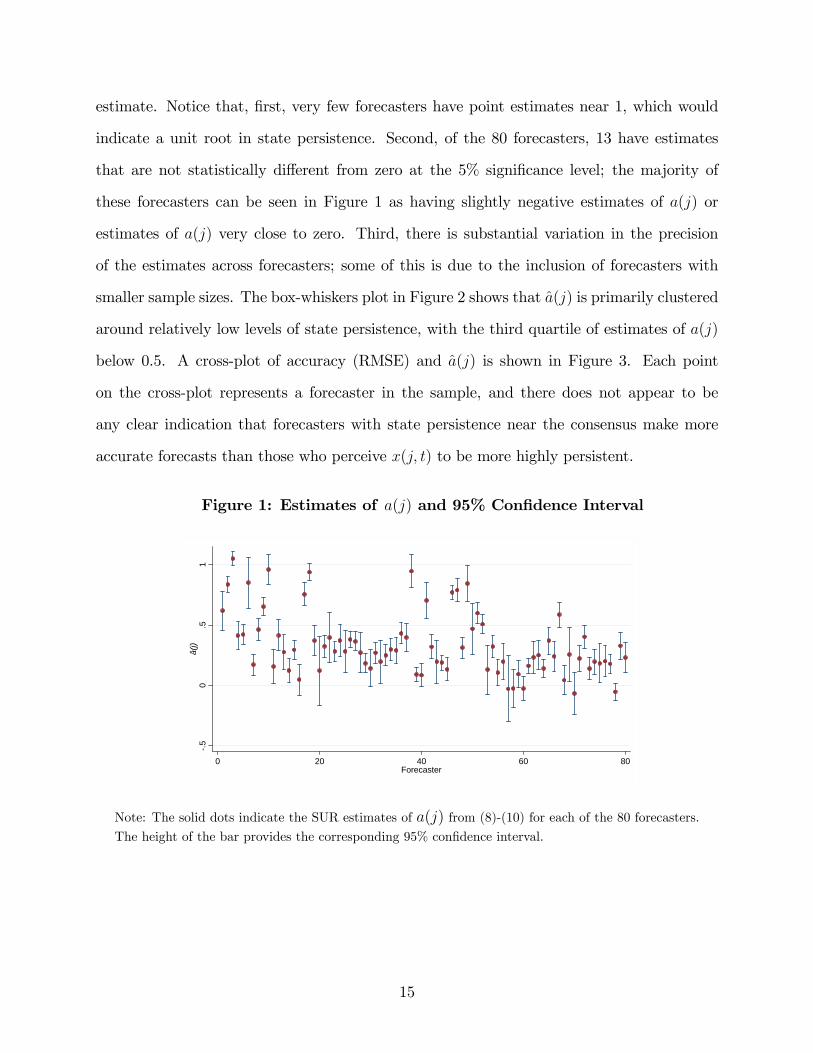
smaller sample sizes. The box-whiskers plot in Figure 2 shows that a(j) is primarily clustered
around relatively low levels of state persistence, with the third quartile of estimates of a(j)
below 0.5. A cross-plot of accuracy (RMSE) and a(j) is shown in Figure 3. Each point
on the cross-plot represents a forecaster in the sample, and there does not appear to be
any clear indication that forecasters with state persistence near the consensus make more
accurate forecasts than those who perceive x(j, t) to be more highly persistent.
Figure 1: Estimates of a(j) and 95% Confidence Interval
.50
.51
â(j)
0 20 40 60 80Forecaster
Note: The solid dots indicate the SUR estimates of a(j) from (8)-(10) for each of the 80 forecasters.
The height of the bar provides the corresponding 95% confidence interval.
15
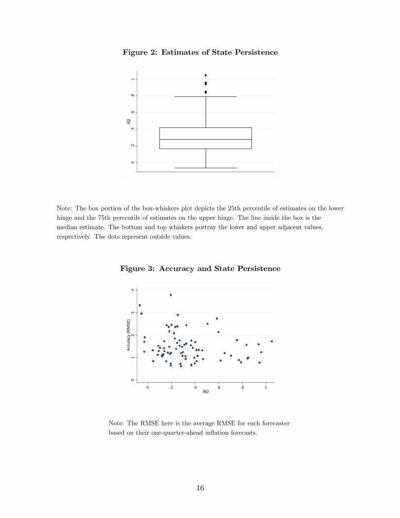
Figure 2: Estimates of State Persistence
0.2
.4.6
.81
â(j)
Note: The box portion of the box-whiskers plot depicts the 25th percentile of estimates on the lower
hinge and the 75th percentile of estimates on the upper hinge. The line inside the box is the
median estimate. The bottom and top whiskers portray the lower and upper adjacent values,
respectively. The dots represent outside values.
Figure 3: Accuracy and State Persistence
01
23
4A
ccur
acy
(RM
SE
)
0 .2 .4 .6 .8 1â(j)
Note: The RMSE here is the average RMSE for each forecaster
based on their one-quarter-ahead inflation forecasts.
16
5.2 Changes in state persistence over time
5.2.1 Split sample estimation
It is possible that state persistence has changed over time. Along with the debate surrounding
the degree of actual inflation persistence, its stability over time remains controversial. Studies
by Levin and Piger (2004) and Stock and Watson (2007) have investigated structural breaks
in the inflation process.
Ideally, a long span of survey participation would allow us to test for breaks in state
persistence with an unknown breakpoint and for individual forecasters, but, given the gaps in
the data set, that is not viable in our case. One way to account for possible changes in state
persistence over time is to perform split sample estimation, splitting the sample roughly in
half. The midway point in our sample would be 1996Q4. However, a group of new forecasters
entered in 1995Q2 and, to avoid splitting their observations after only six quarters, I pick
a split date of 1995Q2. Splitting the sample in this way yields 40 forecasters in the first
portion of the sample (pre-1995Q2) and 53 forecasters in the second (post-1995Q2). Figure
4a shows a smoothed histogram of state persistence point estimates across forecasters, where
the dashed kernel density represents the estimates in the pre-1995Q2 sample and the solid
kernel density represents the estimates in the post-1995Q2 sample. The estimation results
are consistent with those in the literature, which suggests that there has been a decline in
inflation persistence over time. Prior to the mid-1990s, there appeared to be two types of
forecasters: those with high state persistence and those with lower state persistence. That
is, forecasters likely responded to recent macroeconomic news differently and had different
views on the credibility of the central bank. By the mid-1990s, the group of ‘sceptical’
forecasters had decreased. Of course, there is a different composition of forecasters in both
portions of the sample, but the more recent consensus is clearly one of low state persistence.
Given papers that have documented disagreement in inflation expectations across forecasters
(e.g., Capistran and Timmermann (2009); Mankiw, Reis and Wolfers (2003)), this finding
17
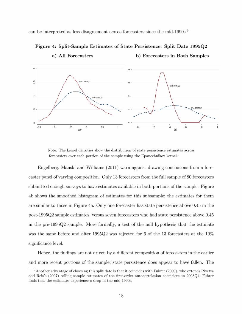
can be interpreted as less disagreement across forecasters since the mid-1990s.9
Figure 4: Split-Sample Estimates of State Persistence: Split Date 1995Q2
a) All Forecasters b) Forecasters in Both Samples
Pre1995Q2
Post1995Q2
0.5
11.
52
.25 0 .25 .5 .75 1â(j)
01
23
40 .2 .4 .6 .8 1
â(j)
Pre1995Q2
Post1995Q2
Note: The kernel densities show the distribution of state persistence estimates across
forecasters over each portion of the sample using the Epanechnikov kernel.
Engelberg, Manski and Williams (2011) warn against drawing conclusions from a fore-
caster panel of varying composition. Only 13 forecasters from the full sample of 80 forecasters
submitted enough surveys to have estimates available in both portions of the sample. Figure
4b shows the smoothed histogram of estimates for this subsample; the estimates for them
are similar to those in Figure 4a. Only one forecaster has state persistence above 0.45 in the
post-1995Q2 sample estimates, versus seven forecasters who had state persistence above 0.45
in the pre-1995Q2 sample. More formally, a test of the null hypothesis that the estimate
was the same before and after 1995Q2 was rejected for 6 of the 13 forecasters at the 10%
significance level.
Hence, the findings are not driven by a different composition of forecasters in the earlier
and more recent portions of the sample; state persistence does appear to have fallen. The
9Another advantage of choosing this split date is that it coincides with Fuhrer (2009), who extends Pivettaand Reis’s (2007) rolling sample estimates of the first-order autocorrelation coeffi cient to 2008Q4; Fuhrerfinds that the estimates experience a drop in the mid-1990s.
18
findings are consistent with many studies that have reported that actual inflation persis-
tence has decreased over time (for examples, see Cogley and Sargent (2001); Taylor (2000);
Stock and Watson (2007)), though a more in-depth comparison between perceived inflation
persistence and actual inflation persistence is provided in section 5.3.
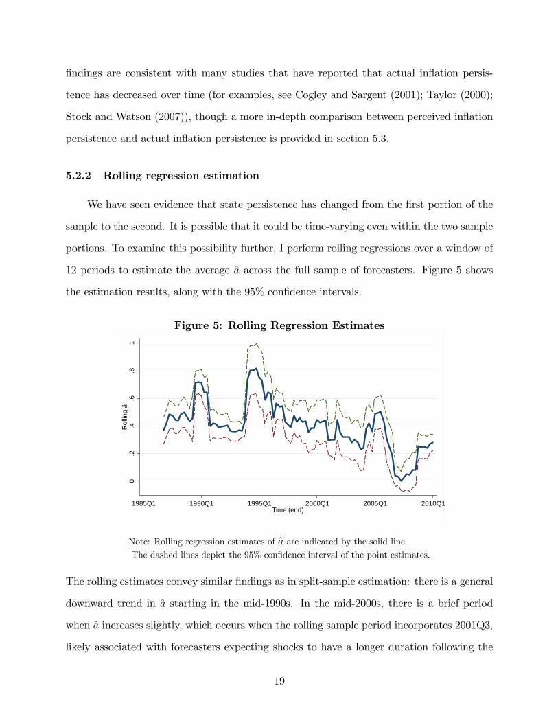
5.2.2 Rolling regression estimation
We have seen evidence that state persistence has changed from the first portion of the
sample to the second. It is possible that it could be time-varying even within the two sample
portions. To examine this possibility further, I perform rolling regressions over a window of
12 periods to estimate the average a across the full sample of forecasters. Figure 5 shows
the estimation results, along with the 95% confidence intervals.
Figure 5: Rolling Regression Estimates
0.2
.4.6
.81
Rol
ling
â
1985Q1 1995Q1 2000Q11990Q1 2010Q12005Q1Time (end)
Note: Rolling regression estimates of a are indicated by the solid line.The dashed lines depict the 95% confidence interval of the point estimates.
The rolling estimates convey similar findings as in split-sample estimation: there is a general
downward trend in a starting in the mid-1990s. In the mid-2000s, there is a brief period
when a increases slightly, which occurs when the rolling sample period incorporates 2001Q3,
likely associated with forecasters expecting shocks to have a longer duration following the
19
September 2001 terrorist attacks. The estimates then fall to very low levels for a brief period,
increasing slightly toward the end of the sample period. Overall, the estimates of a are lower
after the mid-1990s than in the first portion of the sample.
5.3 A comparison with actual inflation data
The measure of state persistence discussed thus far is obtained indirectly using forecast re-
visions. To form a concrete means of comparison with actual inflation data, we can obtain
a measure of perceived inflation persistence by calculating the implied autocorrelation func-
tion (ACF) using the state persistence estimates and comparing it with the ACF of actual
inflation. Fuhrer (2009) advocates use of the ACF to measure persistence, since it summa-
rizes much of the information in the time series. It is defined as the vector of correlations of
current period inflation with each of its own lags from i = 0, 1, 2, .., I: [ρ1, ..., ρI ]. Appendix
D uses the Yule-Walker equations to calculate the following implied autocorrelations for each
forecaster j in the state-space model:
ρ1(j) =γπ1γπ0=
σ2η(j)a(j)3
σ2η(j) + σ2ε(j)[1− a(j)2](11)
ρ2(j) =γπ2γπ0=
σ2η(j)a(j)4
σ2η(j) + σ2ε(j)[1− a(j)2](12)
...
ρi(j) =γπiγπ0=
σ2η(j)a(j)2+i
σ2η(j) + σ2ε(j)[1− a(j)2], (13)
where ρi(j) denotes the implied autocorrelation for forecaster j at lag i. In general, we can
show that
ρi(j) = a(j)ρi−1(j) ∀ i > 2. (14)
At any lag, these autocorrelations depend on a(j) and both shock variances σ2η(j) and σ2ε(j).
If we can obtain sample estimates of σ2ε(j) and σ2η(j), we can identify our measure of perceived
20
inflation persistence.10 Taking expectations from the state-space model yields
Ejtπ(t+ 1) = Ejtx(j, t+ 1) = a(j)x(j, t),
and using the sample estimates of a(j), we can back out an estimate of the state variable:
x(j, t) =Ejtπ(t+ 1)
a(j). (15)
Then, from the measurement equation in the state-space model, we have
ε(j, t) = π(t)− x(j, t) = π(t)− Ejtπ(t+ 1)
a(j), (16)
and therefore,
σ2ε(j) =1
n− 1n∑t=1
ε(j, t)2, j = 1, ..., J. (17)
Similarly, rearranging the transition equation in terms of sample estimates gives
η(j, t) = x(j, t)− a(j)x(j, t− 1) = Ejtπ(t+ 1)
a(j)− Ejt−1π(t). (18)
Thus, computing η(j, t) requires that forecasts be submitted in at least two consecutive
periods. We can then calculate the corresponding variance estimate:
σ2η(j) =1
n− 1n∑t=1
η(j, t)2, j = 1, ..., J. (19)
Figure 6 shows the perceived inflation persistence estimates. Each connected line rep-
resents a different forecaster in the sample, while the successive dots represent lag i. For
the majority of forecasters, the implied autocorrelations start with ρ1(j) < 0.2.11 ,12 This is
10Please see Appendix C(II) for further details related to the sample estimates of the shock variances.11State persistence is typically larger than the perceived inflation persistence, primarily as a result of a
large σ2ε(j) for the vast majority of forecasters.12It could be argued that the use of the short-term, current period, forecast revision, r(j, t, 1), in estimation
21
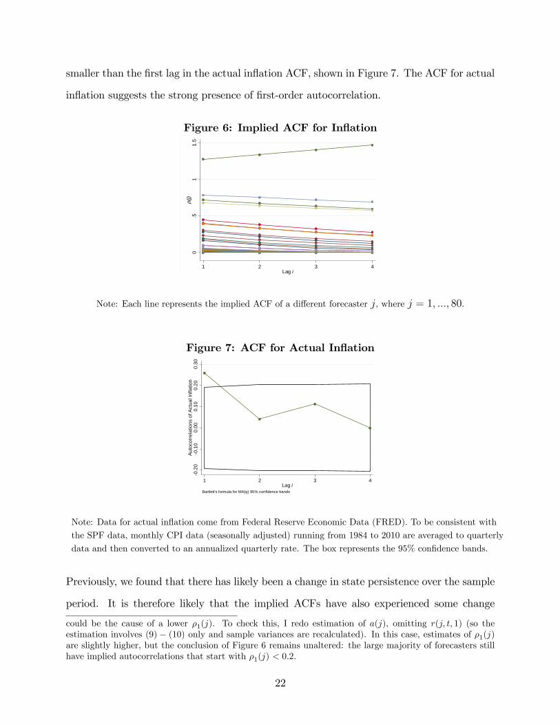
smaller than the first lag in the actual inflation ACF, shown in Figure 7. The ACF for actual
inflation suggests the strong presence of first-order autocorrelation.
Figure 6: Implied ACF for Inflation
0.5
11.
5ρ i
(j)
1 2 3 4Lag i
Note: Each line represents the implied ACF of a different forecaster j, where j = 1, ..., 80.
Figure 7: ACF for Actual Inflation
0.2
00
.10
0.00
0.10
0.20
0.30
Auto
corr
elat
ions
of A
ctua
l Inf
latio
n
1 2 3 4Lag i
Bartlett's formula for MA(q) 95% confidence bands
Note: Data for actual inflation come from Federal Reserve Economic Data (FRED). To be consistent with
the SPF data, monthly CPI data (seasonally adjusted) running from 1984 to 2010 are averaged to quarterly
data and then converted to an annualized quarterly rate. The box represents the 95% confidence bands.
Previously, we found that there has likely been a change in state persistence over the sample
period. It is therefore likely that the implied ACFs have also experienced some change
could be the cause of a lower ρ1(j). To check this, I redo estimation of a(j), omitting r(j, t, 1) (so theestimation involves (9) − (10) only and sample variances are recalculated). In this case, estimates of ρ1(j)are slightly higher, but the conclusion of Figure 6 remains unaltered: the large majority of forecasters stillhave implied autocorrelations that start with ρ1(j) < 0.2.
22
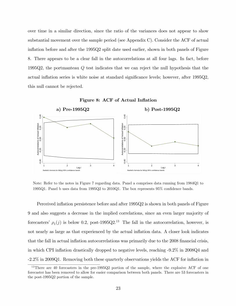
over time in a similar direction, since the ratio of the variances does not appear to show
substantial movement over the sample period (see Appendix C). Consider the ACF of actual
inflation before and after the 1995Q2 split date used earlier, shown in both panels of Figure
8. There appears to be a clear fall in the autocorrelations at all four lags. In fact, before
1995Q2, the portmanteau Q test indicates that we can reject the null hypothesis that the
actual inflation series is white noise at standard significance levels; however, after 1995Q2,
this null cannot be rejected.
Figure 8: ACF of Actual Inflation
a) Pre-1995Q2 b) Post-1995Q2
0.4
00
.20
0.00
0.20
0.40
Auto
corr
elat
ions
of A
ctua
l Inf
latio
n
1 2 3 4Lag i
Bartlett's formula for MA(q) 95% confidence bands
0.4
00
.20
0.00
0.20
0.40
Auto
corr
elat
ions
of A
ctua
l Inf
latio
n
1 2 3 4Lag i
Bartlett's formula for MA(q) 95% confidence bands
Note: Refer to the notes in Figure 7 regarding data. Panel a comprises data running from 1984Q1 to
1995Q1. Panel b uses data from 1995Q2 to 2010Q1. The box represents 95% confidence bands.
Perceived inflation persistence before and after 1995Q2 is shown in both panels of Figure
9 and also suggests a decrease in the implied correlations, since an even larger majority of
forecasters’ρ1(j) is below 0.2, post-1995Q2.13 The fall in the autocorrelation, however, is
not nearly as large as that experienced by the actual inflation data. A closer look indicates
that the fall in actual inflation autocorrelations was primarily due to the 2008 financial crisis,
in which CPI inflation drastically dropped to negative levels, reaching -9.2% in 2008Q4 and
-2.2% in 2009Q1. Removing both these quarterly observations yields the ACF for inflation in
13There are 40 forecasters in the pre-1995Q2 portion of the sample, where the explosive ACF of oneforecaster has been removed to allow for easier comparison between both panels. There are 53 forecasters inthe post-1995Q2 portion of the sample.
23
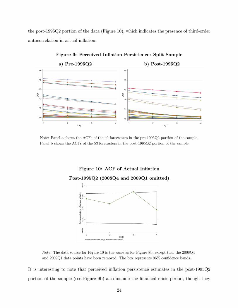
the post-1995Q2 portion of the data (Figure 10), which indicates the presence of third-order
autocorrelation in actual inflation.
Figure 9: Perceived Inflation Persistence: Split Sample
a) Pre-1995Q2 b) Post-1995Q2
0.2
.4.6
.81
ρ i(j)
1 2 3 4Lag i
0.2
.4.6
.81
ρ i(j)
1 2 3 4Lag i
Note: Panel a shows the ACFs of the 40 forecasters in the pre-1995Q2 portion of the sample.
Panel b shows the ACFs of the 53 forecasters in the post-1995Q2 portion of the sample.
Figure 10: ACF of Actual Inflation
Post-1995Q2 (2008Q4 and 2009Q1 omitted)
0.4
00
.20
0.00
0.20
0.40
Auto
corr
elat
ions
of A
ctua
l Inf
latio
n
1 2 3 4Lag i
Bartlett's formula for MA(q) 95% confidence bands
Note: The data source for Figure 10 is the same as for Figure 8b, except that the 2008Q4
and 2009Q1 data points have been removed. The box represents 95% confidence bands.
It is interesting to note that perceived inflation persistence estimates in the post-1995Q2
portion of the sample (see Figure 9b) also include the financial crisis period, though they
24
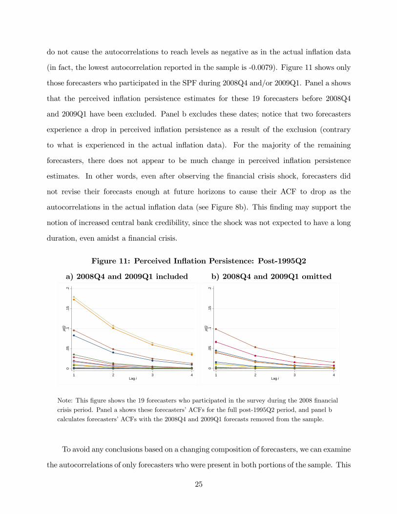
do not cause the autocorrelations to reach levels as negative as in the actual inflation data
(in fact, the lowest autocorrelation reported in the sample is -0.0079). Figure 11 shows only
those forecasters who participated in the SPF during 2008Q4 and/or 2009Q1. Panel a shows
that the perceived inflation persistence estimates for these 19 forecasters before 2008Q4
and 2009Q1 have been excluded. Panel b excludes these dates; notice that two forecasters
experience a drop in perceived inflation persistence as a result of the exclusion (contrary
to what is experienced in the actual inflation data). For the majority of the remaining
forecasters, there does not appear to be much change in perceived inflation persistence
estimates. In other words, even after observing the financial crisis shock, forecasters did
not revise their forecasts enough at future horizons to cause their ACF to drop as the
autocorrelations in the actual inflation data (see Figure 8b). This finding may support the
notion of increased central bank credibility, since the shock was not expected to have a long
duration, even amidst a financial crisis.
Figure 11: Perceived Inflation Persistence: Post-1995Q2
a) 2008Q4 and 2009Q1 included b) 2008Q4 and 2009Q1 omitted
0.0
5.1
.15
.2ρ i
(j)
1 2 3 4Lag i
0.0
5.1
.15
.2ρ i
(j)
1 2 3 4Lag i
Note: This figure shows the 19 forecasters who participated in the survey during the 2008 financial
crisis period. Panel a shows these forecasters’ACFs for the full post-1995Q2 period, and panel b
calculates forecasters’ACFs with the 2008Q4 and 2009Q1 forecasts removed from the sample.
To avoid any conclusions based on a changing composition of forecasters, we can examine
the autocorrelations of only forecasters who were present in both portions of the sample. This
25
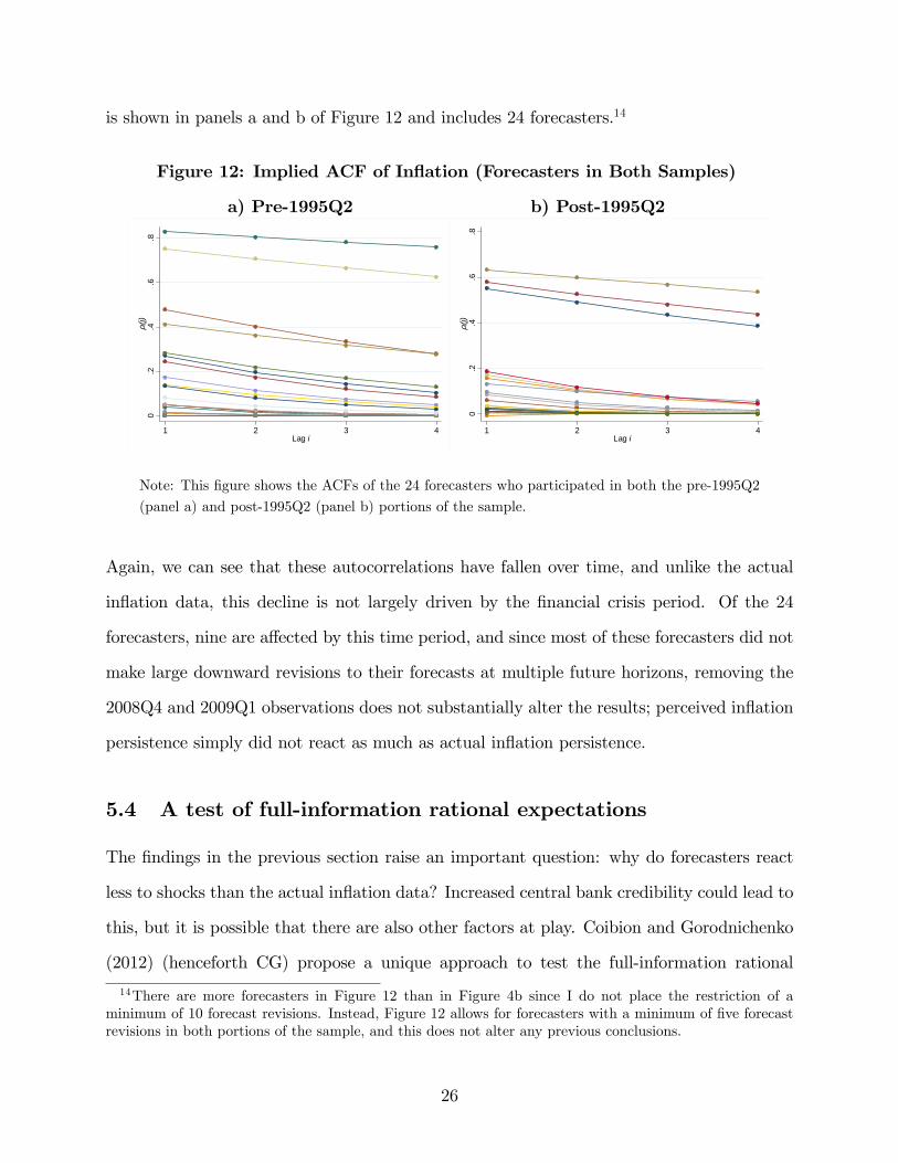
is shown in panels a and b of Figure 12 and includes 24 forecasters.14
Figure 12: Implied ACF of Inflation (Forecasters in Both Samples)
a) Pre-1995Q2 b) Post-1995Q2
0.2
.4.6
.8ρ i
(j)
1 2 3 4Lag i
0.2
.4.6
.8ρ i
(j)
1 2 3 4Lag i
Note: This figure shows the ACFs of the 24 forecasters who participated in both the pre-1995Q2
(panel a) and post-1995Q2 (panel b) portions of the sample.
Again, we can see that these autocorrelations have fallen over time, and unlike the actual
inflation data, this decline is not largely driven by the financial crisis period. Of the 24
forecasters, nine are affected by this time period, and since most of these forecasters did not
make large downward revisions to their forecasts at multiple future horizons, removing the
2008Q4 and 2009Q1 observations does not substantially alter the results; perceived inflation
persistence simply did not react as much as actual inflation persistence.
5.4 A test of full-information rational expectations
The findings in the previous section raise an important question: why do forecasters react
less to shocks than the actual inflation data? Increased central bank credibility could lead to
this, but it is possible that there are also other factors at play. Coibion and Gorodnichenko
(2012) (henceforth CG) propose a unique approach to test the full-information rational
14There are more forecasters in Figure 12 than in Figure 4b since I do not place the restriction of aminimum of 10 forecast revisions. Instead, Figure 12 allows for forecasters with a minimum of five forecastrevisions in both portions of the sample, and this does not alter any previous conclusions.
26
expectations (FIRE) hypothesis. This approach can identify whether a rejection of FIRE
arises due to informational rigidities. Alternatively, a rejection could occur as a result of a
deviation from rational expectations. I employ tests along the lines of CG to gain insight
into the underlying reason why forecasters’perceptions of inflation persistence differ from
actual inflation persistence. It is worth noting that although much of this paper has focused
on obtaining forecaster-specific results, the tests proposed by CG apply only when averaging
across agents, and are therefore not expected to hold at the individual level. Hence, the
results reported here will be based on the average of the sample of 80 forecasters studied in
this paper.
CG show that models of informational rigidities imply the following relationship between
ex-post mean forecast errors and ex-ante mean forecast revisions:
χ(t+ h)− Etχ(t+ h) = c+ β[Etχ(t+ h)− Et−1χ(t+ h)] + error(t),
where χ is a given macroeconomic variable, and Eχ is the mean forecast across agents. CG
find that when β > 0, informational rigidities are present. Models of informational rigidities
also predict a constant of zero.
I test the following relationship between average h-quarter-ahead inflation forecast errors
across forecasters and the corresponding average forecast revisions for h = 1, 2, 3:
π(t+ h)− Etπ(t+ h) = c(h) + β(h)[Etπ(t+ h)− Et−1π(t+ h)] + error(t). (20)
The results are reported in Table 1 for each forecast horizon, with the inclusion of two lagged
quarterly changes in real oil prices (as in CG). In panel a, at horizon 1, the coeffi cient on
forecast revisions is positive, though statistically significant only at the 15% level. When
h = 2, β2 is statistically significant, but in the opposite direction than what would be implied
by informational rigidities. Furthermore, in both cases, the first lag of log changes in real
oil prices is statistically significant at the 5% level, which should not be the case in the
27
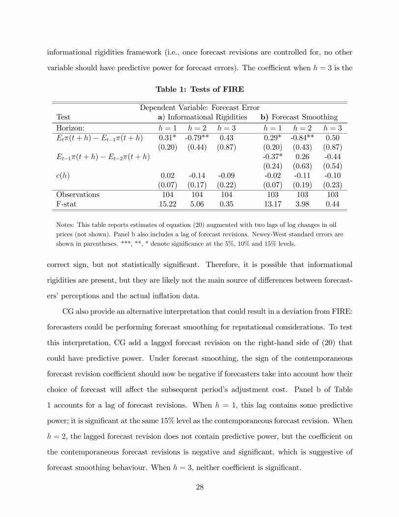
informational rigidities framework (i.e., once forecast revisions are controlled for, no other
variable should have predictive power for forecast errors). The coeffi cient when h = 3 is the
Table 1: Tests of FIRE
Dependent Variable: Forecast ErrorTest a) Informational Rigidities b) Forecast SmoothingHorizon: h = 1 h = 2 h = 3 h = 1 h = 2 h = 3Etπ(t+ h)− Et−1π(t+ h) 0.31* -0.79** 0.43 0.29* -0.84** 0.50
(0.20) (0.44) (0.87) (0.20) (0.43) (0.87)Et−1π(t+ h)− Et−2π(t+ h) -0.37* 0.26 -0.44
(0.24) (0.63) (0.54)c(h) 0.02 -0.14 -0.09 -0.02 -0.11 -0.10
(0.07) (0.17) (0.22) (0.07) (0.19) (0.23)Observations 104 104 104 103 103 103F-stat 15.22 5.06 0.35 13.17 3.98 0.44
Notes: This table reports estimates of equation (20) augmented with two lags of log changes in oil
prices (not shown). Panel b also includes a lag of forecast revisions. Newey-West standard errors are
shown in parentheses. ***, **, * denote significance at the 5%, 10% and 15% levels.
correct sign, but not statistically significant. Therefore, it is possible that informational
rigidities are present, but they are likely not the main source of differences between forecast-
ers’perceptions and the actual inflation data.
CG also provide an alternative interpretation that could result in a deviation from FIRE:
forecasters could be performing forecast smoothing for reputational considerations. To test
this interpretation, CG add a lagged forecast revision on the right-hand side of (20) that
could have predictive power. Under forecast smoothing, the sign of the contemporaneous
forecast revision coeffi cient should now be negative if forecasters take into account how their
choice of forecast will affect the subsequent period’s adjustment cost. Panel b of Table
1 accounts for a lag of forecast revisions. When h = 1, this lag contains some predictive
power; it is significant at the same 15% level as the contemporaneous forecast revision. When
h = 2, the lagged forecast revision does not contain predictive power, but the coeffi cient on
the contemporaneous forecast revisions is negative and significant, which is suggestive of
forecast smoothing behaviour. When h = 3, neither coeffi cient is significant.
28
Overall, these results suggest that forecast smoothing is somewhat more likely to be the
source of deviation from FIRE forecasts. Professional forecasters may be required to give a
compelling and well-supported explanation whenever a previous forecast is revised, causing
them to eliminate or dampen the effects of certain shocks in their forecasts, and therefore
lowering estimates of perceived inflation persistence relative to actual inflation persistence.
This differs from the results found in CG, in which the source of deviation from FIRE is due
to informational rigidities. This could be due to several factors: first, the mean measures
used here represent only the 80 forecasters in the SPF that are investigated in this paper,
not the full sample available in the SPF that is used by CG. Second, the estimates here
are reported separately for each forecast horizon, whereas CG pool estimates across forecast
horizons.15 Third, CG’s results are based on GDP/GNP deflator inflation forecasts dating
back to 1968Q4, whereas, here, CPI inflation forecasts dating back to 1984Q1 are used.
6 Conclusions
This paper proposes a new methodology to extract measures of persistence from expectations
data. Empirically, this paper shows that it is possible to estimate a measure of perceived
inflation persistence while allowing for heterogeneity across forecasters and minimal assump-
tions on the models they use. The measure of perceived inflation persistence introduced in
this paper provides important insights into expectations data, and, when used in conjunction
with persistence measures of actual data, can be useful in the arsenal of both researchers
and policy-makers.
Perceived inflation persistence has declined over time, with greater consensus around
low levels of persistence when split sample estimation is performed. These findings are
consistent with those of Stock and Watson (2007), who suggest that unexpected changes
15Pooling horizons would not be consistent with the model presented in this paper, since forecast revisionsin the one-step-ahead case would be a fraction of the two-step-ahead forecast revisions, which, in turn, is afraction of the three-step-ahead forecast revision. Hence, we would not expect β(h) to be the same acrossforecast horizons.
29
to inflation are more likely to be viewed as transitory than they had been before the early
1990s.
From the perspective of a central bank, perceptions of inflation persistence have im-
plications for monetary policy. The relatively lower persistence estimates obtained through
inflation-expectations data appear to suggest that the Federal Reserve has gained credibility
in recent years, giving them greater flexibility, and lowering the costs associated with stabi-
lizing inflation. There may, however, be other factors driving inflation expectations, causing
their underlying properties to differ from those of actual inflation, such as forecasters’incen-
tives to smooth their announced forecasts, leading them to differ from true values. Future
work will aim to examine the testable implications of this perspective.
A natural next step for future research would also entail developing a better understand-
ing of the perceptions of other agents in the economy, such as businesses and the public.
Since the methodology proposed in this paper is applicable in different contexts, given a rich
enough data set, it can be used to obtain measures of perceived inflation persistence that
are comparable across agents. Subsequently, a detailed analysis of the implications of these
results for monetary policy would be a key avenue to explore.
30
References
[1] Andrade, Philippe and Herve Le Bihan. 2010. Inattentive Professional Forecasters. Un-published Manuscript.
[2] Ang, Andrew, Bekaert, Geert and Min Wei. 2007. Do Macro Variables, Asset Markets,or Surveys Forecast Inflation Better? Journal of Monetary Economics, 54: 1163-1212.
[3] Benati, Luca. 2008. Investigating Inflation Persistence across Monetary Regimes. Quar-terly Journal of Economics, 123(3): 1005-1060.
[4] Brainard, William C. and George L. Perry. 2000. Making policy in a changing world.In: Perry, G., Tobin, J. (Eds.), Economic Events, Ideas, and Policies: The 1960s andAfter. Brookings Institution Press, Washington.
[5] Capistran, Carlos and Allan Timmermann. 2009. Disagreement and Biases in InflationExpectations. Journal of Money, Credit and Banking, 41(2-3): 365-396.
[6] Cogley, Timothy and Thomas J. Sargent. 2001. Evolving Post World War II U.S. Infla-tion Dynamics. NBER Macroeconomics Annual, 16: 331-373.
[7] Cogley, Timothy, Primiceri, Giorgio E. and Thomas J. Sargent. 2010. Inflation-GapPersistence in the U.S. American Economic Journal: Macroeconomics, 2(1): 43-69.
[8] Coibion, Olivier and Yuriy Gorodnichenko. 2012. Information Rigidity and the Expec-tations Formation Process: A Simple Framework and New Facts. NBERWorking PaperNo. 16537.
[9] Diebold, Francis X., and Lutz Kilian. 2001. Measuring Predictability: Theory andMacroeconomic Applications. Journal of Applied Econometrics, 16: 657-669.
[10] Engelberg, Joseph, Manski, Charles F., and Jared Williams. 2011. Assessing the Tempo-ral Variation of Macroeconomic Forecasts by a Panel of Changing Composition. Journalof Applied Econometrics. doi: 10.1002/jae.1206.
[11] Faust, Jon and Jonathan H. Wright. 2012. Forecasting Inflation. Johns Hopkins Uni-versity Working Paper.
[12] Fuhrer, Jeffrey C. 2009. Inflation Persistence. Federal Reserve Bank of Boston WorkingPaper No. 09-14.
[13] Gourinchas, Pierre-Olivier and Aaron Tornell. 2004. Exchange Rate Puzzles and Dis-torted Beliefs. Journal of International Economics, 64: 303-333.
[14] Grant, Alan P. and Lloyd B. Thomas. 1999. Inflationary expectations and rationalityrevisited. Economics Letters, 62(3): 331-338.
[15] Jain, Monica. 2010. Estimating Inflation Persistence Implied by Forecast Data. Queen’sUniversity.
31
[16] Krane, Spencer D. 2011. Professional Forecasters’Views of Permanent and TransitoryShocks to GDP. American Economic Journal: Macroeconomics, 3: 184-211.
[17] Levin, Andrew T. and Jeremy M. Piger. 2004. Is Inflation Persistence Intrinsic in In-dustrial Economies? European Central Bank Working Paper Series, No. 334.
[18] Mackowiak, Bartosz and Mirko Wiederholt. 2009. Optimal Sticky Prices under RationalInattention. American Economic Review, 99: 769-803.
[19] Mankiw, Gregory N., Ricardo Reis, and Justin Wolfers (2003). Disagreement aboutInflation Expectations. NBER Macroeconomics Annual, 209-248.
[20] Mehra, Yash P. 2002. Survey Measures of Expected Inflation: Revisiting the Issuesof Predictive Content and Rationality. Federal Reserve Bank of Richmond EconomicQuarterly, 88: 17-36.
[21] Mendes, Rhys and Stephen Murchison. 2009—2010. Declining Inflation Persistence inCanada: Causes and Consequences. Bank of Canada Review (Winter): 1-14.
[22] Patton, Andrew J. and Allan Timmermann. 2010. Why do Forecasters Disagree?Lessons from the Term Structure of Cross-Sectional Dispersion. Journal of MonetaryEconomics, 57: 803-820.
[23] Pivetta, Frederic and Ricardo Reis. 2007. The Persistence of Inflation in the UnitedStates. Journal of Economic Dynamics and Control, 31: 1326-58.
[24] Sims, Christopher A. 2001. Comment on Sargent and Cogley’s ‘Evolving Post WorldWar II U.S. Inflation Dynamics.’NBER Macroeconomics Annual, 16: 373-379.
[25] Sims, Christopher A. 2003. Implications of Rational Inattention. Journal of MonetaryEconomics, 50: 665-690.
[26] Stock, James H. 2001. Discussion of Cogley and Sargent ‘Evolving Post World War IIU.S. Inflation Dynamics.’NBER Macroeconomics Annual, 16: 379-387.
[27] Stock, James H. and Mark W. Watson. 2007. Why Has Inflation Become Harder toForecast? Journal of Money Credit and Banking, 39(1): 3-33.
[28] Taylor, John B. 2000. Low inflation, pass-through, and the pricing power of firms.European Economic Review, 44(7), 1389—1408.
[29] Thomas, Lloyd B. 1999. Survey Measures of Expected U.S. Inflation. Journal of Eco-nomic Perspectives, 13: 125-144.
[30] Woodford, Michael. 2009. Information-Constrained State-Dependent Pricing. Journalof Monetary Economics, 56: S100-S124.
32
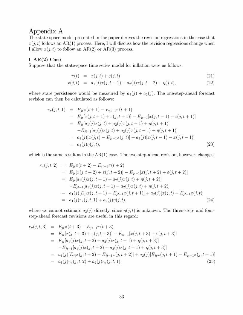
Appendix AThe state-space model presented in the paper derives the revision regressions in the case thatx(j, t) follows an AR(1) process. Here, I will discuss how the revision regressions change whenI allow x(j, t) to follow an AR(2) or AR(3) process.
I. AR(2) CaseSuppose that the state-space time series model for inflation were as follows:
π(t) = x(j, t) + ε(j, t) (21)
x(j, t) = a1(j)x(j, t− 1) + a2(j)x(j, t− 2) + η(j, t), (22)
where state persistence would be measured by a1(j) + a2(j). The one-step-ahead forecastrevision can then be calculated as follows:
rπ(j, t, 1) = Ejtπ(t+ 1)− Ejt−1π(t+ 1)= Ejt[x(j, t+ 1) + ε(j, t+ 1)]− Ejt−1[x(j, t+ 1) + ε(j, t+ 1)]
= Ejt[a1(j)x(j, t) + a2(j)x(j, t− 1) + η(j, t+ 1)]
−Ejt−1[a1(j)x(j, t) + a2(j)x(j, t− 1) + η(j, t+ 1)]
= a1(j)[x(j, t)− Ejt−1x(j, t)] + a2(j)[x(j, t− 1)− x(j, t− 1)]= a1(j)η(j, t), (23)
which is the same result as in the AR(1) case. The two-step-ahead revision, however, changes:
rπ(j, t, 2) = Ejtπ(t+ 2)− Ejt−1π(t+ 2)= Ejt[x(j, t+ 2) + ε(j, t+ 2)]− Ejt−1[x(j, t+ 2) + ε(j, t+ 2)]
= Ejt[a1(j)x(j, t+ 1) + a2(j)x(j, t) + η(j, t+ 2)]
−Ejt−1[a1(j)x(j, t+ 1) + a2(j)x(j, t) + η(j, t+ 2)]
= a1(j)[Ejtx(j, t+ 1)− Ejt−1x(j, t+ 1)] + a2(j)[x(j, t)− Ejt−1x(j, t)]= a1(j)rπ(j, t, 1) + a2(j)η(j, t), (24)
where we cannot estimate a2(j) directly, since η(j, t) is unknown. The three-step- and four-step-ahead forecast revisions are useful in this regard:
rπ(j, t, 3) = Ejtπ(t+ 3)− Ejt−1π(t+ 3)= Ejt[x(j, t+ 3) + ε(j, t+ 3)]− Ejt−1[x(j, t+ 3) + ε(j, t+ 3)]
= Ejt[a1(j)x(j, t+ 2) + a2(j)x(j, t+ 1) + η(j, t+ 3)]
−Ejt−1[a1(j)x(j, t+ 2) + a2(j)x(j, t+ 1) + η(j, t+ 3)]
= a1(j)[Ejtx(j, t+ 2)− Ejt−1x(j, t+ 2)] + a2(j)[Ejtx(j, t+ 1)− Ejt−1x(j, t+ 1)]= a1(j)rπ(j, t, 2) + a2(j)rπ(j, t, 1), (25)
33
rπ(j, t, 4) = Ejtπ(t+ 4)− Ejt−1π(t+ 4)= Ejt[x(j, t+ 4) + ε(j, t+ 4)]− Ejt−1[x(j, t+ 4) + ε(j, t+ 4)]
= Ejt[a1(j)x(j, t+ 3) + a2(j)x(j, t+ 2) + η(j, t+ 4)]
−Ejt−1[a1(j)x(j, t+ 3) + a2(j)x(j, t+ 2) + η(j, t+ 4)]
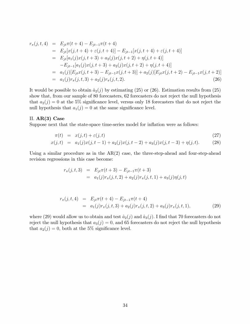
= a1(j)[Ejtx(j, t+ 3)− Ejt−1x(j, t+ 3)] + a2(j)[Ejtx(j, t+ 2)− Ejt−1x(j, t+ 2)]= a1(j)rπ(j, t, 3) + a2(j)rπ(j, t, 2). (26)
It would be possible to obtain a2(j) by estimating (25) or (26). Estimation results from (25)show that, from our sample of 80 forecasters, 62 forecasters do not reject the null hypothesisthat a2(j) = 0 at the 5% significance level, versus only 18 forecasters that do not reject thenull hypothesis that a1(j) = 0 at the same significance level.
II. AR(3) CaseSuppose next that the state-space time-series model for inflation were as follows:
π(t) = x(j, t) + ε(j, t) (27)
x(j, t) = a1(j)x(j, t− 1) + a2(j)x(j, t− 2) + a3(j)x(j, t− 3) + η(j, t). (28)
Using a similar procedure as in the AR(2) case, the three-step-ahead and four-step-aheadrevision regressions in this case become:
rπ(j, t, 3) = Ejtπ(t+ 3)− Ejt−1π(t+ 3)= a1(j)rπ(j, t, 2) + a2(j)rπ(j, t, 1) + a3(j)η(j, t)
rπ(j, t, 4) = Ejtπ(t+ 4)− Ejt−1π(t+ 4)= a1(j)rπ(j, t, 3) + a2(j)rπ(j, t, 2) + a3(j)rπ(j, t, 1), (29)
where (29) would allow us to obtain and test a2(j) and a3(j). I find that 70 forecasters do notreject the null hypothesis that a3(j) = 0, and 65 forecasters do not reject the null hypothesisthat a2(j) = 0, both at the 5% significance level.
34
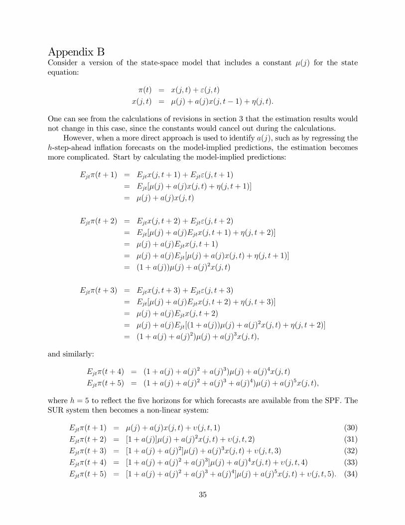
Appendix BConsider a version of the state-space model that includes a constant µ(j) for the stateequation:
π(t) = x(j, t) + ε(j, t)
x(j, t) = µ(j) + a(j)x(j, t− 1) + η(j, t).
One can see from the calculations of revisions in section 3 that the estimation results wouldnot change in this case, since the constants would cancel out during the calculations.
However, when a more direct approach is used to identify a(j), such as by regressing theh-step-ahead inflation forecasts on the model-implied predictions, the estimation becomesmore complicated. Start by calculating the model-implied predictions:
Ejtπ(t+ 1) = Ejtx(j, t+ 1) + Ejtε(j, t+ 1)
= Ejt[µ(j) + a(j)x(j, t) + η(j, t+ 1)]
= µ(j) + a(j)x(j, t)
Ejtπ(t+ 2) = Ejtx(j, t+ 2) + Ejtε(j, t+ 2)
= Ejt[µ(j) + a(j)Ejtx(j, t+ 1) + η(j, t+ 2)]
= µ(j) + a(j)Ejtx(j, t+ 1)
= µ(j) + a(j)Ejt[µ(j) + a(j)x(j, t) + η(j, t+ 1)]
= (1 + a(j))µ(j) + a(j)2x(j, t)
Ejtπ(t+ 3) = Ejtx(j, t+ 3) + Ejtε(j, t+ 3)
= Ejt[µ(j) + a(j)Ejtx(j, t+ 2) + η(j, t+ 3)]
= µ(j) + a(j)Ejtx(j, t+ 2)
= µ(j) + a(j)Ejt[(1 + a(j))µ(j) + a(j)2x(j, t) + η(j, t+ 2)]
= (1 + a(j) + a(j)2)µ(j) + a(j)3x(j, t),
and similarly:
Ejtπ(t+ 4) = (1 + a(j) + a(j)2 + a(j)3)µ(j) + a(j)4x(j, t)
Ejtπ(t+ 5) = (1 + a(j) + a(j)2 + a(j)3 + a(j)4)µ(j) + a(j)5x(j, t),
where h = 5 to reflect the five horizons for which forecasts are available from the SPF. TheSUR system then becomes a non-linear system:
Ejtπ(t+ 1) = µ(j) + a(j)x(j, t) + υ(j, t, 1) (30)
Ejtπ(t+ 2) = [1 + a(j)]µ(j) + a(j)2x(j, t) + υ(j, t, 2) (31)
Ejtπ(t+ 3) = [1 + a(j) + a(j)2]µ(j) + a(j)3x(j, t) + υ(j, t, 3) (32)
Ejtπ(t+ 4) = [1 + a(j) + a(j)2 + a(j)3]µ(j) + a(j)4x(j, t) + υ(j, t, 4) (33)
Ejtπ(t+ 5) = [1 + a(j) + a(j)2 + a(j)3 + a(j)4]µ(j) + a(j)5x(j, t) + υ(j, t, 5). (34)
35
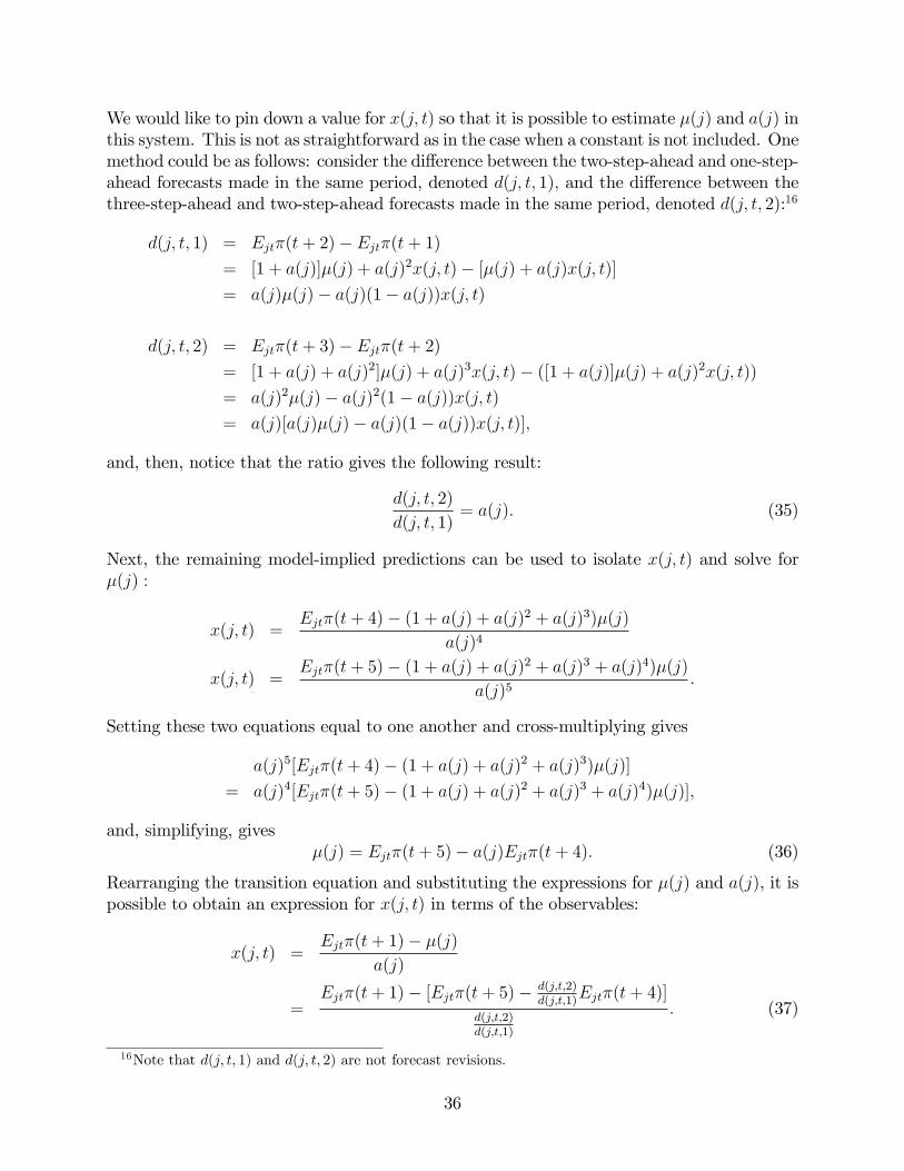
We would like to pin down a value for x(j, t) so that it is possible to estimate µ(j) and a(j) inthis system. This is not as straightforward as in the case when a constant is not included. Onemethod could be as follows: consider the difference between the two-step-ahead and one-step-ahead forecasts made in the same period, denoted d(j, t, 1), and the difference between thethree-step-ahead and two-step-ahead forecasts made in the same period, denoted d(j, t, 2):16
d(j, t, 1) = Ejtπ(t+ 2)− Ejtπ(t+ 1)= [1 + a(j)]µ(j) + a(j)2x(j, t)− [µ(j) + a(j)x(j, t)]
= a(j)µ(j)− a(j)(1− a(j))x(j, t)
d(j, t, 2) = Ejtπ(t+ 3)− Ejtπ(t+ 2)= [1 + a(j) + a(j)2]µ(j) + a(j)3x(j, t)− ([1 + a(j)]µ(j) + a(j)2x(j, t))
= a(j)2µ(j)− a(j)2(1− a(j))x(j, t)= a(j)[a(j)µ(j)− a(j)(1− a(j))x(j, t)],
and, then, notice that the ratio gives the following result:
d(j, t, 2)
d(j, t, 1)= a(j). (35)
Next, the remaining model-implied predictions can be used to isolate x(j, t) and solve forµ(j) :
x(j, t) =Ejtπ(t+ 4)− (1 + a(j) + a(j)2 + a(j)3)µ(j)
a(j)4
x(j, t) =Ejtπ(t+ 5)− (1 + a(j) + a(j)2 + a(j)3 + a(j)4)µ(j)
a(j)5.
Setting these two equations equal to one another and cross-multiplying gives
a(j)5[Ejtπ(t+ 4)− (1 + a(j) + a(j)2 + a(j)3)µ(j)]
= a(j)4[Ejtπ(t+ 5)− (1 + a(j) + a(j)2 + a(j)3 + a(j)4)µ(j)],
and, simplifying, givesµ(j) = Ejtπ(t+ 5)− a(j)Ejtπ(t+ 4). (36)
Rearranging the transition equation and substituting the expressions for µ(j) and a(j), it ispossible to obtain an expression for x(j, t) in terms of the observables:
x(j, t) =Ejtπ(t+ 1)− µ(j)
a(j)
=Ejtπ(t+ 1)− [Ejtπ(t+ 5)− d(j,t,2)
d(j,t,1)Ejtπ(t+ 4)]
d(j,t,2)d(j,t,1)
. (37)
16Note that d(j, t, 1) and d(j, t, 2) are not forecast revisions.
36
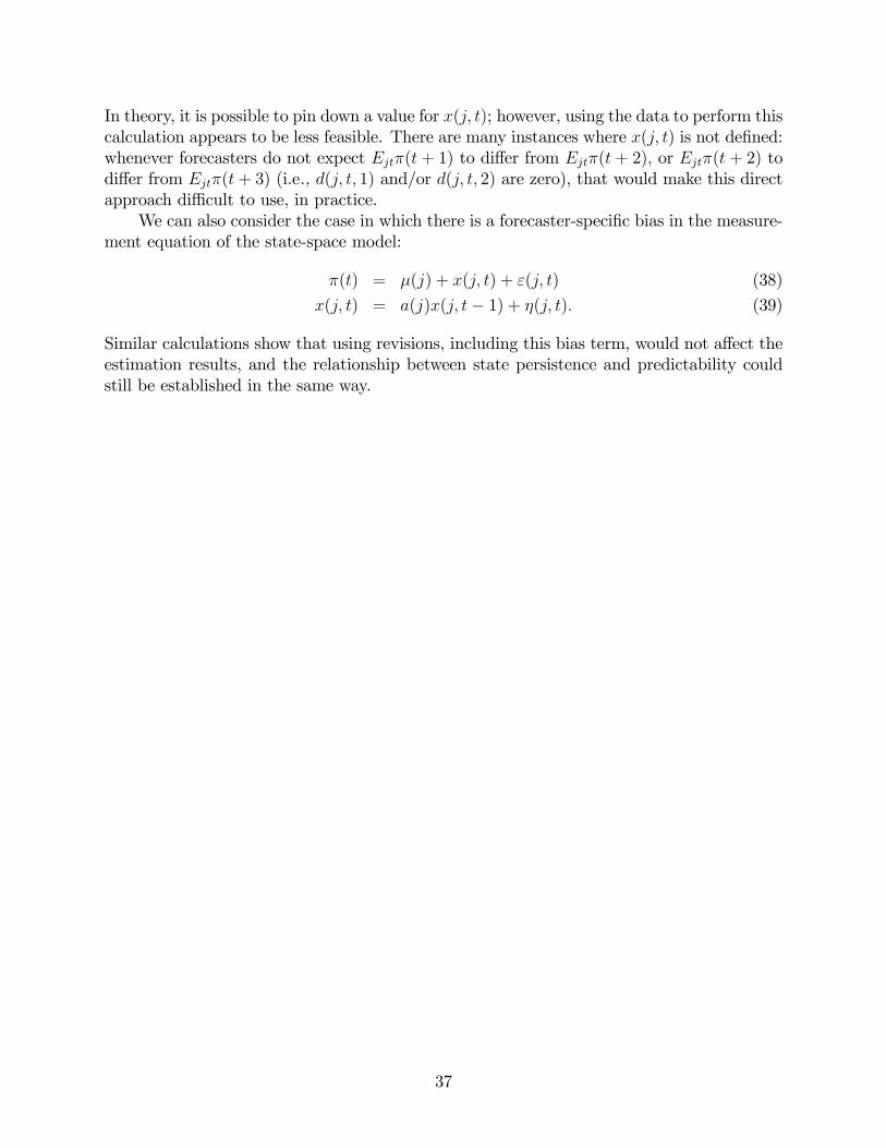
In theory, it is possible to pin down a value for x(j, t); however, using the data to perform thiscalculation appears to be less feasible. There are many instances where x(j, t) is not defined:whenever forecasters do not expect Ejtπ(t + 1) to differ from Ejtπ(t + 2), or Ejtπ(t + 2) todiffer from Ejtπ(t+ 3) (i.e., d(j, t, 1) and/or d(j, t, 2) are zero), that would make this directapproach diffi cult to use, in practice.
We can also consider the case in which there is a forecaster-specific bias in the measure-ment equation of the state-space model:
π(t) = µ(j) + x(j, t) + ε(j, t) (38)
x(j, t) = a(j)x(j, t− 1) + η(j, t). (39)
Similar calculations show that using revisions, including this bias term, would not affect theestimation results, and the relationship between state persistence and predictability couldstill be established in the same way.
37
Appendix C
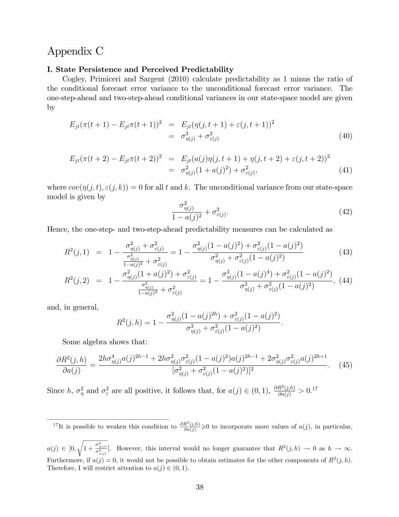
I. State Persistence and Perceived PredictabilityCogley, Primiceri and Sargent (2010) calculate predictability as 1 minus the ratio of
the conditional forecast error variance to the unconditional forecast error variance. Theone-step-ahead and two-step-ahead conditional variances in our state-space model are givenby
Ejt(π(t+ 1)− Ejtπ(t+ 1))2 = Ejt(η(j, t+ 1) + ε(j, t+ 1))2
= σ2η(j) + σ2ε(j) (40)
Ejt(π(t+ 2)− Ejtπ(t+ 2))2 = Ejt(a(j)η(j, t+ 1) + η(j, t+ 2) + ε(j, t+ 2))2
= σ2η(j)(1 + a(j)2) + σ2ε(j), (41)
where cov(η(j, t), ε(j, k)) = 0 for all t and k. The unconditional variance from our state-spacemodel is given by
σ2η(j)1− a(j)2 + σ2ε(j). (42)
Hence, the one-step- and two-step-ahead predictability measures can be calculated as
R2(j, 1) = 1−σ2η(j) + σ2ε(j)σ2η(j)
1−a(j)2 + σ2ε(j)
= 1−σ2η(j)(1− a(j)2) + σ2ε(j)(1− a(j)2)
σ2η(j) + σ2ε(j)(1− a(j)2)(43)
R2(j, 2) = 1−σ2η(j)(1 + a(j)2) + σ2ε(j)
σ2η(j)
1−a(j)2 + σ2ε(j)
= 1−σ2η(j)(1− a(j)4) + σ2ε(j)(1− a(j)2)
σ2η(j) + σ2ε(j)(1− a(j)2), (44)
and, in general,
R2(j, h) = 1−σ2η(j)(1− a(j)2h) + σ2ε(j)(1− a(j)2)
σ2η(j) + σ2ε(j)(1− a(j)2).
Some algebra shows that:
∂R2(j, h)
∂a(j)=2hσ4η(j)a(j)
2h−1 + 2hσ2η(j)σ2ε(j)(1− a(j)2)a(j)2h−1 + 2σ2η(j)σ2ε(j)a(j)2h+1
[σ2η(j) + σ2ε(j)(1− a(j)2)]2. (45)
Since h, σ2η and σ2ε are all positive, it follows that, for a(j) ∈ (0, 1),
∂R2(j,h)∂a(j)
> 0.17
17It is possible to weaken this condition to ∂R2(j,h)∂a(j) >0 to incorporate more values of a(j), in particular,
a(j) ∈ [0,√1 +
σ2η(j)
σ2ε(j)
]. However, this interval would no longer guarantee that R2(j, h) → 0 as h → ∞.
Furthermore, if a(j) = 0, it would not be possible to obtain estimates for the other components of R2(j, h).Therefore, I will restrict attention to a(j) ∈ (0, 1).
38
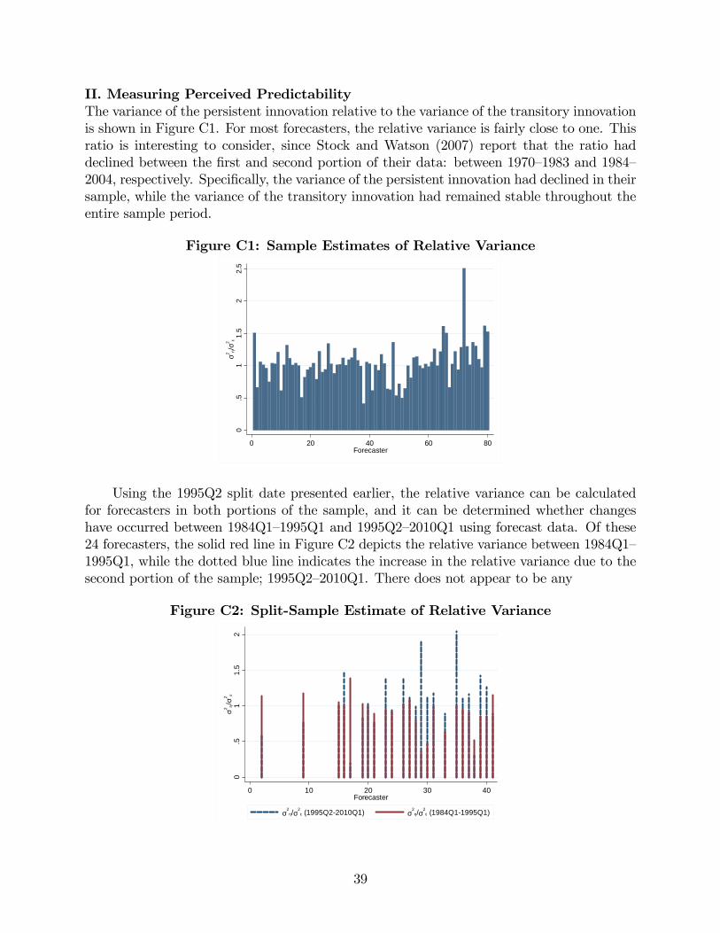
II. Measuring Perceived PredictabilityThe variance of the persistent innovation relative to the variance of the transitory innovationis shown in Figure C1. For most forecasters, the relative variance is fairly close to one. Thisratio is interesting to consider, since Stock and Watson (2007) report that the ratio haddeclined between the first and second portion of their data: between 1970—1983 and 1984—2004, respectively. Specifically, the variance of the persistent innovation had declined in theirsample, while the variance of the transitory innovation had remained stable throughout theentire sample period.
Figure C1: Sample Estimates of Relative Variance0
.51
1.5
22.
5σ2 η
/σ2 ε
0 20 40 60 80Forecaster
Using the 1995Q2 split date presented earlier, the relative variance can be calculatedfor forecasters in both portions of the sample, and it can be determined whether changeshave occurred between 1984Q1—1995Q1 and 1995Q2—2010Q1 using forecast data. Of these24 forecasters, the solid red line in Figure C2 depicts the relative variance between 1984Q1—1995Q1, while the dotted blue line indicates the increase in the relative variance due to thesecond portion of the sample; 1995Q2—2010Q1. There does not appear to be any
Figure C2: Split-Sample Estimate of Relative Variance
0.5
11.
52
σ2 η/σ
2 ε
0 10 20 30 40Forecaster
σ2
η/σ2
ε (1995Q22010Q1) σ2
η/σ2
ε (1984Q11995Q1)
39
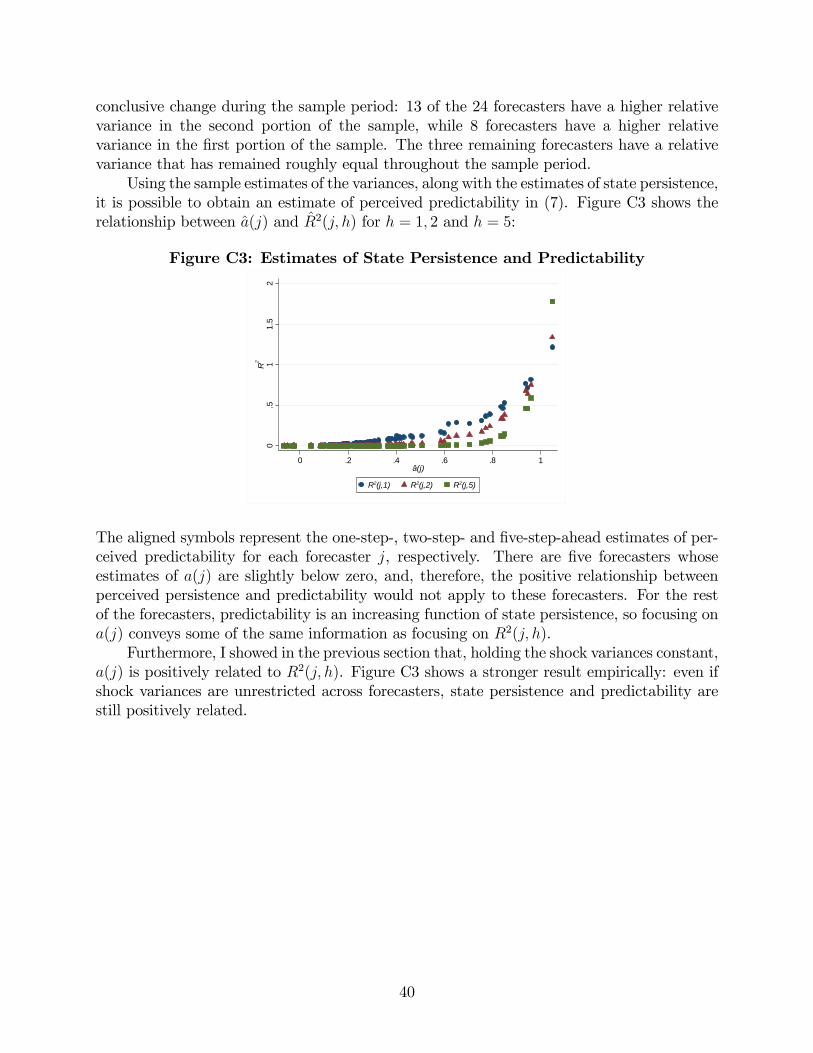
conclusive change during the sample period: 13 of the 24 forecasters have a higher relativevariance in the second portion of the sample, while 8 forecasters have a higher relativevariance in the first portion of the sample. The three remaining forecasters have a relativevariance that has remained roughly equal throughout the sample period.
Using the sample estimates of the variances, along with the estimates of state persistence,it is possible to obtain an estimate of perceived predictability in (7). Figure C3 shows therelationship between a(j) and R2(j, h) for h = 1, 2 and h = 5:
Figure C3: Estimates of State Persistence and Predictability0
.51
1.5
2R
2
0 .2 .4 .6 .8 1â(j)
R2(j,1) R2(j,2) R2(j,5)
The aligned symbols represent the one-step-, two-step- and five-step-ahead estimates of per-ceived predictability for each forecaster j, respectively. There are five forecasters whoseestimates of a(j) are slightly below zero, and, therefore, the positive relationship betweenperceived persistence and predictability would not apply to these forecasters. For the restof the forecasters, predictability is an increasing function of state persistence, so focusing ona(j) conveys some of the same information as focusing on R2(j, h).
Furthermore, I showed in the previous section that, holding the shock variances constant,a(j) is positively related to R2(j, h). Figure C3 shows a stronger result empirically: even ifshock variances are unrestricted across forecasters, state persistence and predictability arestill positively related.
40
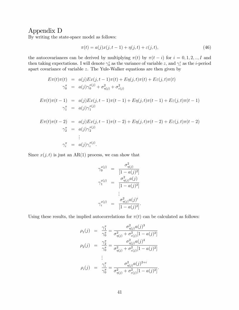
Appendix DBy writing the state-space model as follows:
π(t) = a(j)x(j, t− 1) + η(j, t) + ε(j, t), (46)
the autocovariances can be derived by multiplying π(t) by π(t − i) for i = 0, 1, 2, .., I andthen taking expectations. I will denote γz0 as the variance of variable z, and γ
zi as the i-period
apart covariance of variable z. The Yule-Walker equations are then given by
Eπ(t)π(t) = a(j)Ex(j, t− 1)π(t) + Eη(j, t)π(t) + Eε(j, t)π(t)
γπ0 = a(j)γx(j)0 + σ2η(j) + σ2ε(j)
Eπ(t)π(t− 1) = a(j)Ex(j, t− 1)π(t− 1) + Eη(j, t)π(t− 1) + Eε(j, t)π(t− 1)γπ1 = a(j)γ
x(j)1
Eπ(t)π(t− 2) = a(j)Ex(j, t− 1)π(t− 2) + Eη(j, t)π(t− 2) + Eε(j, t)π(t− 2)γπ2 = a(j)γ
x(j)2
...
γπi = a(j)γx(j)i .
Since x(j, t) is just an AR(1) process, we can show that
γx(j)0 =
σ2η(j)[1− a(j)2]
γx(j)1 =
σ2η(j)a(j)
[1− a(j)2]...
γx(j)i =
σ2η(j)a(j)i
[1− a(j)2] .
Using these results, the implied autocorrelations for π(t) can be calculated as follows:
ρ1(j) =γπ1γπ0=
σ2η(j)a(j)3
σ2η(j) + σ2ε(j)[1− a(j)2]
ρ2(j) =γπ2γπ0=
σ2η(j)a(j)4
σ2η(j) + σ2ε(j)[1− a(j)2]...
ρi(j) =γπiγπ0=
σ2η(j)a(j)2+i
σ2η(j) + σ2ε(j)[1− a(j)2].
41