Federal Reserve Bank of New YorkStaff Reports

Trend Inflation and Inflation Persistence in the New Keynesian Phillips Curve

Timothy CogleyArgia M. Sbordone

Staff Report no. 270December 2006

This paper presents preliminary findings and is being distributed to economistsand other interested readers solely to stimulate discussion and elicit comments.The views expressed in the paper are those of the authors and are not necessarilyreflective of views at the Federal Reserve Bank of New York or the FederalReserve System. Any errors or omissions are the responsibility of the authors.

Trend Inflation and Inflation Persistence in the New Keynesian Phillips CurveTimothy Cogley and Argia M. SbordoneFederal Reserve Bank of New York Staff Reports, no. 270December 2006JEL classification: E31

Abstract

The New Keynesian Phillips curve (NKPC) asserts that inflation depends onexpectationsof real marginal costs, but empirical research has shown that purelyforward-looking versions of the model generate too little inflation persistence. In thispaper, we offer a resolution of the persistence problem. We hypothesize that inflation ishighly persistent because of drift in trend inflation, a feature that many versions of theNKPC neglect. We derive a version of the NKPC as a log-linear approximation around a time-varying inflation trend and examine whether it explains deviations of inflationfrom that trend. We estimate the NKPC parameters jointly with those that define theinflation trend by estimating a vector autoregression with drifting coefficients andvolatilities; the autoregressive parameters are constrained to satisfy the restrictionsimposed by the NKPC. Our results suggest that trend inflation has been historicallyquite volatile and that a purely forward-looking model that takes these fluctuations into account approximates well the short-run dynamics of inflation.

Key words: inflation persistence, Phillips curve, time-varying VAR

Cogley: University of California, Davis (twcogley@ucdavis.edu). Sbordone: Federal ReserveBank of New York (argia.sbordone@ny.frb.org). For comments and suggestions, the authorsthank Jean Boivin, Mark Gertler, Peter Ireland, Sharon Kozicki, Jim Nason, Luca Sala,Dan Waggoner, Michael Woodford, Tao Zha, and two anonymous referees. They also thankseminar participants at the November 2005 NBER Monetary Economics meeting, the October2005 Conference on Quantitative Models at the Federal Reserve Bank of Cleveland, the 2004Society for Computational Economics Meeting in Amsterdam, the Federal Reserve's Fall 2004Macro System Committee Meeting in Baltimore, the Federal Reserve Bank of New York, theFederal Reserve Bank of Richmond, and Duke University. The views expressed in this paperare those of the authors and do not necessarily reflect the position of the Federal ReserveBank of New York or the Federal Reserve System.

1 Introduction

In this paper we ask two questions. First, to what extent can Calvo’s (1983) model

of nominal price rigidities explain inflation dynamics without relying on arbitrary

backward-looking terms? Second, is the implied relationship between inflation and

marginal cost stable over time? The relevance of these questions is hardly overstated,

for Calvo’s model is a widely-used building block for the aggregate supply curve of

modern dynamic macromodels.

In its baseline formulation, the Calvo model leads to a purely forward-looking New

Keynesian Phillips curve (NKPC): inflation depends on the expected evolution of

real marginal costs. However, purely forward-looking models are deemed inconsistent

with empirical evidence of significant inflation persistence (e.g., see Fuhrer and Moore

1995). Accordingly, a number of authors have added backward-looking elements to

enhance the degree of inflation persistence in the model and provide a better fit with

aggregate data. Lags of inflation are typically introduced by postulating some form of

price indexation (e.g., see Christiano et al. 2005) or rule-of-thumb behavior (e.g., see

Gali and Gertler 1999). These mechanisms have been criticized because they lack a

convincing microeconomic foundation; price indexation also counters the observation

that many prices do indeed remain constant in monetary terms for several periods

(e.g., see Bils and Klenow 2004).

We think that this apparent inflation persistence problem could be resolved by

being clear about what features of inflation the model is supposed to explain. The

NKPC is really a model of the inflation gap, i.e. the difference between actual and

trend inflation. In most formulations, however, this distinction vanishes because the

NKPC is obtained by log-linearizing equilibrium conditions around a steady state

characterized by zero trend inflation. The conventional approximation is useful for

normative studies because trend inflation should be close to zero under an optimal

monetary policy rule. But log-linearizing around zero inflation can be problematic for

fitting data from monetary regimes in which trend inflation is far from zero, especially

if trend inflation is also highly variable.

Variation in trend inflation is important for understanding inflation persistence.

For the U.S., a number of authors model trend inflation as a driftless random walk

(e.g., see Cogley and Sargent 2005a, Ireland 2006, and Stock and Watson 2006).

Thus trend inflation contributes a highly persistent component to actual inflation.

1

But this persistence arises from a source that is distinct from the NKPC. In general

equilibrium, trend inflation is determined by the long-run target in the central bank’s

policy rule, and drift in trend inflation is usually attributed to shifts in that target.

Most existing versions of the NKPC abstract from this source of variation.1 Since

they neglect what is probably the most persistent component of inflation, it is not

surprising that they struggle to account fully for inflation persistence.

In this paper we extend the Calvo model to incorporate variation in trend in-

flation. We log-linearize the equilibrium conditions of the model around a steady

state characterized by a time-varying inflation trend. The resulting representation is

a log-linear NKPC with time-varying coefficients, which we estimate using Bayesian

methods. Our econometric approach exploits the cross-equation restrictions that the

model imposes on a vector autoregression for inflation and unit labor costs. Following

Cogley and Sargent (2005a), the V AR has drifting parameters and stochastic volatil-

ity, but here the conditional mean parameters are constrained to satisfy the model’s

cross-equation restrictions. We jointly estimate the Calvo pricing parameters along

with those of the V AR; while the former are ultimately those of interest, we use the

V AR parameters to construct estimates of trend inflation.

We investigate whether a purely forward-looking version of the model can be rec-

onciled with the data and also how variation in trend inflation affects the NKPC

coefficients. Our estimates point to four conclusions. First, there is significant ev-

idence of drift in trend inflation. Second, a purely forward-looking version of the

model explains quite well the dynamics of the inflation gap: the posterior for the

backward-looking indexation parameter clusters near zero, and a Bayesian measure

of model fit favors a purely forward-looking specification over a hybrid representa-

tion. Third, our estimates of the frequency of price adjustment are in accord with

the micro evidence of Bils and Klenow (2004). Finally, variation in trend inflation

alters the relative weights on current and future marginal cost in the NKPC: as

trend inflation increases, the weight on forward-looking terms is enhanced, while that

on current marginal cost is muted.

The rest of the paper is organized as follows. The next section extends the Calvo

model. Section 3 describes the econometric approach and characterizes the cross-

1This is true for most single equation models. A number of recent general equilibrium modelsthat include some form of NKPC allow variation in trend inflation and compute the inflation gapaccordingly (e.g., see Ireland 2006, Smets and Wouters 2003, Schorfheide 2005).

2

equation restrictions. Section 4 discusses data and priors, and section 5 presents and

discusses the results. Section 6 concludes with suggestions for future research.

2 A Calvo model with drifting trend inflation

We start with a standard version of the Calvo model, with monopolistic competi-

tion and random intervals between price changes. To investigate the importance of a

backward-looking term, we allow prices that are not re-optimized to partially catch-

up with lagged inflation. This assumption is consistent with the hypothesis that

the price adjustment process involves essentially information-gathering costs rather

than menu costs. We also assume that capital cannot be instantaneously reallocated

across firms, and therefore take into account a discrepancy between individual and

aggregate marginal costs.2

We depart from traditional derivations of the Calvo model, however, in allowing

for a shifting trend inflation process, which we model as a driftless random walk.

As a consequence, when we approximate the non-linear equilibrium conditions of the

model, we take the log-linear approximation, in each period, around a steady state

associated with a time-varying rate of trend inflation. As usual, this approximation

is only valid for small deviations of the variables from their steady state. This mod-

ification brings with it another important departure from the standard assumptions

that we discuss in more detail below. When trend inflation varies over time, we have

to take a stand about the evolution of agents’ expectations: we therefore replace

the assumption of rational expectation with one of subjective expectations and make

appropriate assumptions on how subjective beliefs evolve over time.

The importance of trend inflation for the dynamics of the Calvo model was brought

to attention by Ascari (2004), and has been subsequently analyzed in various con-

tributions (see Kiley 2004, Ascari and Ropele 2006, Sahuc 2006, and Bakhshi et al.

2003, among others). This literature has shown that there is a constraint on the

maximum level of trend inflation in order for a solution to the model to exist, and

also that the level of trend inflation affects the dynamics of the Phillips curve, unless

a sufficient degree of indexation is allowed.

2Here we also implicitly assume, as in Sbordone (2002), that capital is exogenous. For a dis-cussion of the implications of endogenous firm-specific capital for the NKPC see Woodford (2005).Eichenbaum and Fisher (2004), Altig et al. (2005) and Matheron (2005) discuss the implications ofendogenous firm-specific capital on the estimated frequency of price adjustment in empiricalNKPC.

3

We go beyond these analyses in two respects. First, we model trend inflation as

time-varying, and derive the Calvo equation under this assumption: this allows us

to map the evolving level of trend inflation into NKPC coefficients that vary over

time. Furthermore, we take the model to the data, so that we can identify periods

of high and low trend inflation and estimate the Calvo parameters, which we take to

be the primitives of the model.3 Estimates of these parameters and of trend inflation

allow us to describe the evolution of the NKPC coefficients. These estimates should

be relevant for the analysis of DSGE models that allow for a time-varying inflation

target.4 Existing models in the literature can ignore the implications of time varying

trend inflation in the NKPC because they either assume full indexation, or assume

a mixed form of indexation, part to past inflation and part to trend inflation. We

believe that our analysis contributes to a better understanding of these models.

In the rest of this section we summarize the generalized Calvo model, and report

the log-linearized solution; details of the derivation are in appendix A.

Firms i that set prices optimally choose nominal price Xt to maximize expected

discounted future profits5

maxXt

eEtΣjαj {Qt,t+jΠt+j} (1)

where Πt+j = Π(XtΨtj, Pt+j, Yt+j(i), Yt+j), subject to the demand constraint

Yt+j(i) = Yt+j

µXtΨtj

Pt+j

¶−θ. (2)

We denote by eEt subjective expectations formed with time t information, by (1− α)

the probability of setting prices optimally, with 0 < α < 1, by Pt ≡hR 10Pt (i)

1−θ dii 11−θ

the aggregate price level and by Yt ≡hR 10Yt(i)

(θ−1)/θdiiθ/(θ−1)

a measure of aggregate

real output, where Yt(i) is firms’ i output. Qt,t+j is a nominal discount factor between

time t and t+ j; θ [0,∞) is the Dixit-Stiglitz elasticity of substitution among dif-ferentiated goods, and XtΨtj/Pt+j is the relative price at t + j of the firms that set

3In a companion paper (Cogley and Sbordone 2005) we study whether the assumption of timeinvariant Calvo coefficients holds in the data.

4See for example the DSGE models of Adolfson et al. (2005), Ireland (2006), Schorfheide (2005)and Smets and Wouters (2003, 2005), which make different hypotheses about the specific drivingprocess of the inflation target.

5Since each firm that change prices solves the same problem, this price is the same for all thefirms and therefore need not be indexed by i.

4

price at t. The variable Ψtj, defined as

Ψtj =

½1 j = 0,

Πj−1k=0πt+k j ≥ 1, , (3)

captures the fact that individual firm prices that are not set optimally evolve accord-

ing to

Pt(i) = πt−1Pt−1(i), (4)

where πt = Pt/Pt−1 is the gross rate of inflation and [0, 1] is the indexation

parameter.

The firms’ first order conditions are

eEt

∞Xj=0

αjQt,t+jYt+jPθt+jΨ

1−θtj

µXt − θ

θ − 1MCt+j,tΨ−1tj

¶= 0, (5)

whereMCt+j,t is the nominal marginal cost at t+ j of the firm that changes its price

at t. Since we assume immobile capital, this cost differs from the average marginal

cost at time t+ j, MCt+j, creating a form of strategic complementarity.6 Finally, the

evolution of aggregate prices is

Pt =£(1− α)X1−θ

t + α(πt−1Pt−1)1−θ¤ 11−θ . (6)

To obtain the NKPC we log-linearize the equilibrium conditions (5) and (6) around

a steady state characterized by a shifting trend inflation, which we denote by πt.

To work with stationary variables we define by eπt the ratio of inflation to its trend(eπt ≡ πt/πt) , which in steady state is unity, and by gπt the rate of growth of inflation

trend (gπt ≡ πt/πt−1). We then appropriately transform conditions (5) and (6) in

terms of these variables in order to proceed with the log-linearization. We use a

bar over a variable to indicate its value in steady state, and a hat to denote its

log-deviations from steady state.

The inflation equation that we obtain7 can be written in a familiar recursive form

as bπt = et ¡bπt−1 − bgπt ¢+ ζtcmct + b1t eEtbπt+1 + b2t eEt

X∞j=2

ϕj−11t bπt+j + ut, (7)

6The specific relation between firm’s and aggregate marginal cost is in eq. (28) in Appendix A.Strategic complementarity reduces the aggregate price adjustment even when the fraction of stickyprices is small.

7The main steps of the derivation are in Appendix A. A more detailed appendix is available fromthe authors upon request.

5

where bπt ≡ ln eπt = ln (πt/πt) and cmct = ln(mct/mct). We include an error term

ut to account for the fact that this equation is an approximation and to allow for

other possible mis-specifications. Compared with the standard NKPC, obtained as

an approximation around zero inflation (a point where πt = 1 for all t), the right-

hand side of (7) includes innovations to trend inflation bgπt as well as additional leads ofexpected inflation.8 The standard NKPC emerges as a special case when steady-state

inflation is zero or when there is full indexation ( = 1).

TheNKPC coefficients et, ζt, b1t, b2t, and ϕ1t are functions of the Calvo parametersand of trend inflation; formulas are given in equation (48) of appendix A. Comparing

the coefficients with those in the standard model reveals two things. First, when

trend inflation drifts, the coefficients of (7) are time varying (provided 6= 1). This istrue despite the fact that the underlying Calvo parameters α, , and θ are assumed to

be constant. In other words, the NKPC can have time-varying parameters even when

the frequency of price adjustment, the extent of indexation to past inflation, and the

elasticity of demand are constant. Second, equation (7) includes inflation expectations

farther into the future: their exclusion in traditional Calvo equations may be the

source of omitted-variable bias in the estimate of the coefficients of marginal cost and

lagged inflation, should the omitted terms be correlated with the included ones. We

comment more on this comparison later.

3 Empirical methodology

Our objective is to estimate the Calvo coefficients in an environment that al-

lows for drift in trend inflation. We are especially interested in comparing hybrid

and purely forward-looking versions of the NKPC and examining whether a purely

forward-looking specification fits adequately once shifts in trend inflation are taken

into account.

We have in mind an environment in which agents’ subjective beliefs evolve over

time as they learn about changes in monetary policy that affect the long-run trend

of inflation. Firms set prices in accordance with the NKPC, but with a forecasting

model whose parameters drift as their beliefs evolve. We represent their forecasting

8The loglinear approximation actually includes some additional terms involving expectations ofqt and the rate of output growth. In previous work (Cogley and Sbordone 2005), however, we foundthat the coefficient multiplying those terms was close to zero (see also Ascari 2004). Because themodel is already difficult to estimate, we simplify it by dropping those nuisance terms.

6

model as a time-varying vector autoregression. If inflation is determined in accordance

with the NKPC, that vector autoregression should satisfy a collection of nonlinear

cross-equation restrictions.

Our econometric analysis focuses on the restricted V AR process:

yt = X 0tϑ(φt, ψ) +R

1/2t ξt, (8)

where the vector yt includes labor share and inflation,Xt consists of constants plus two

lags of yt, ξt is a standard normal innovation, and Rt is a stochastic volatility matrix.

The function ϑ(·) represents a vector of restricted conditional mean parameters thatdepend on two lower-dimensional parameter vectors φt and ψ = [α, , θ]. The function

ϑ(·) encodes the model’s cross-equation restrictions.This representation combines elements of Cogley and Sargent (2005a) and Sbor-

done (2002, 2005). From Cogley and Sargent, we borrow drifting parameters and

stochastic volatility. Our specification (8) is similar to theirs, with one exception:

here the drifting parameters φt represent a subset of the conditional mean parame-

ters ϑ(φt, ψ). The vector φt includes the V AR intercepts along with the autoregressive

parameters of the labor share equation. The remaining elements of ϑ(φt, ψ) — viz.

the autoregressive parameters of the inflation equation — are pinned down by the

cross-equation restrictions.

Following Cogley and Sargent (2005a), we assume that φt evolves as a driftless

random walk. The transition density,

f(φt+1|φt, S) = N(φt, S), (9)

makes φt+1 conditionally normal with mean φt and variance S. We also assume that

innovations to φt are independent of the standardized V AR innovations ξt and the

volatility innovations ηit in (11) below. The innovation variance Rt is

Rt = B−1HtB−10, (10)

whereHt is diagonal and B is lower triangular with 1’s on the diagonal. The elements

of Ht are assumed to be independent, univariate stochastic volatility processes that

evolve as driftless, geometric random walks,

lnhit = lnhit−1 + σiηit. (11)

The innovation ηit is a standard normal variate, orthogonal to ηjt, and independent

of the other shocks in the model. This specification permits recurrent permanent

7

changes in variances, it allows a time-varying correlation between the V AR innova-

tions, and it ensures that Rt is positive definite.

The V AR provides an internal measure of trend inflation. Following Beveridge

and Nelson (1981), we define trend inflation as the level to which inflation is expected

to settle after short-run fluctuations die out, lnπt = limj→∞Et lnπt+j.9 We write (8)

in companion form,

zt = µt +Atzt−1 + εzt, (12)

where At are the autoregressive parameters of ϑ(φt, ψ). We assume that agents use

(12) to form expectations at date t− 1: the parameters µt and At therefore represent

their beliefs. The one-step ahead V AR forecast of πt is e0πAtbzt−1, where bzt = zt− µzt

and µzt = (I −At)−1µt. We approximate trend inflation as

ln πt = e0π(I −At)−1µt, (13)

where ek is a selection vector that picks up variable k in vector zt.

Trend inflation ultimately depends on φt and ψ, and it is estimated jointly with the

other parameters of the model. Notice that ln πt is a driftless random walk to a first-

order approximation: this follows from the fact that a first-order Taylor expansion

makes ln πt linear in φt, which evolves as a driftless random walk.

From Sbordone (2002), we borrow the cross-equation restrictions that the NKPC

imposes on a reduced-form V AR. To characterize those restrictions, we project both

sides of equation (7) onto bzt−1. The left-hand side is just the V AR forecast of inflation,e0πAtbzt−1. The right-hand side is a structural forecast of inflation implied by theNKPC. If the NKPC is a correct representation of the data, the two conditional

expectations should coincide.

Evaluating the right-hand side involves multi-step forecasts of inflation, which are

difficult to evaluate when parameters drift. But as expectations represents subjec-

tive beliefs, we invoke an approximation that is standard in the learning literature

in macroeconomics (e.g., see Evans and Honkapohja 2001): we assume that agents

treat drifting parameters as if they would remain constant at the current level go-

ing forward in time. Kreps (1998) refers to this as an ‘anticipated-utility’ model,

and he recommends it as a way to model bounded rationality. Cogley and Sargent

(2006) defend it as an approximation to Bayesian forecasting and decision making in

9In the model, π represents gross inflation, and bπt = lnπt− lnπt. That is why the VAR estimateis expressed in terms of ln(π).

8

high-dimensional state spaces. That approximation is very good in models that as-

sume certainty equivalence. Our formulation implicitly assumes certainty equivalence

because we log-linearize the firm’s first-order conditions.

Using the anticipated-utility approximation, multi-step forecasts can be expressed

in the usual way in terms of powers of At:eEt−1bzt+j = eEt−1(At+jAt+j−1...At)bzt−1 .= Aj+1

t bzt−1. (14)

With this assumption and after some algebra, the NKPC inflation forecast can be

expressed as

eEt−1πt = [ete0π + ζte0mcAt + b1te

0πA

2t + b2te

0πϕ1t(I − ϕ1tAt)

−1A3t ]bzt−1. (15)

Terms involving ut drop out because the cost-push shock is assumed to be white

noise. Similarly, bgπt drops out because this is the innovation to trend inflation and isa martingale difference.

The cross-equation restrictions follow from equating the two forecasts,

e0πAtbzt−1 = [ete0π + ζte0mcAt + b1te

0πA

2t + b2te

0πϕ1t(I − ϕ1tAt)

−1A3t ]bzt−1. (16)

To ensure that this holds for any realization of zt−1, the parameters must satisfy

e0πAt = ete0πI + ζt e0mcAt + b1te

0πA

2t + b2te

0πϕ1t(I − ϕ1tAt)

−1A3t . (17)

The left-hand side represents the autoregressive parameters in the V AR inflation

equation. The right-hand side involves all the elements of At as well as the NKPC

parameters. The latter depend in turn on the Calvo parameters ψ as well as trend

inflation, which itself depends on At. Equation (17) therefore represents a collection

of nonlinear cross-equation restrictions which constrain the elements of At to be

functions of φt and ψ. The function ϑ(φt, ψ) represents a vector of V AR parameters

that satisfies (17).

Thus, we estimate a drifting-parameter V AR that is subject to nonlinear cross-

equation restrictions. Appendix B describes Markov Chain Monte Carlo methods for

simulating the joint posterior for this model.

4 Data and Priors

As noted above, the model depends on the joint behavior of inflation and real

marginal cost. Inflation is measured from the implicit GDP deflator, recorded in

9

NIPA table 1.3.4, and marginal cost is approximated by unit labor cost. This is

correct under the hypothesis of Cobb-Douglas technology: in this case the marginal

product of labor is proportional to the average product, and real marginal cost (rmct)

is proportional to unit labor cost,

rmct = wtHt/(1− a)PtYt = (1− a)−1ulct, (18)

where (1− a) is the output elasticity to hours of work in the production function. A

standard calibration for (1− a) is 0.7, and we use that value to transform ulct into

rmct.

Unit labor cost is measured in the same way as in Cogley and Sbordone (2005). We

begin by computing an index of total compensation in the non-farm business sector

from BLS indices of nominal compensation and total hours of work, then translate

the result into dollars. A (log) measure of real unit labor cost ulc is then obtained

by subtracting (log of) nominal GDP from (log of) labor compensation. The new

measure of ulc correlates almost perfectly with the BLS index number for unit labor

cost in the non-farm business sector, another measure commonly used in the literature

(e.g., see Sbordone 2002, 2005). The current measure is useful because it gives unit

labor cost in its natural units rather than as index number.

Both variables are sampled quarterly starting in 1947.Q1 and ending in 2003.Q4.

Data for the first 12 years are used to calibrate the prior, and the remainder are used

to simulate the posterior.

Next we describe the prior. We assume that parameters and initial states are

independent across blocks, so that the joint prior can be expressed as the product of

marginal priors. Then we separately calibrate each of the marginal priors.

Table 1 summarizes our prior on the structural parameters α, β, θ, , and ω. For

β and ω, we have quite strong beliefs. Our assumptions about technology imply that

the strategic complementarity parameter ω = a/(1 − a). Since the output elasticity

1− a should be close to 0.7, it follows that ω must be close to ω = 0.3/0.7 = 0.4286.

Similarly, the discount factor β should be close to 0.99. Because we have strong priors

about these two parameters and our model is so complex, we decided to simplify by

calibrating β and ω at those values.

10

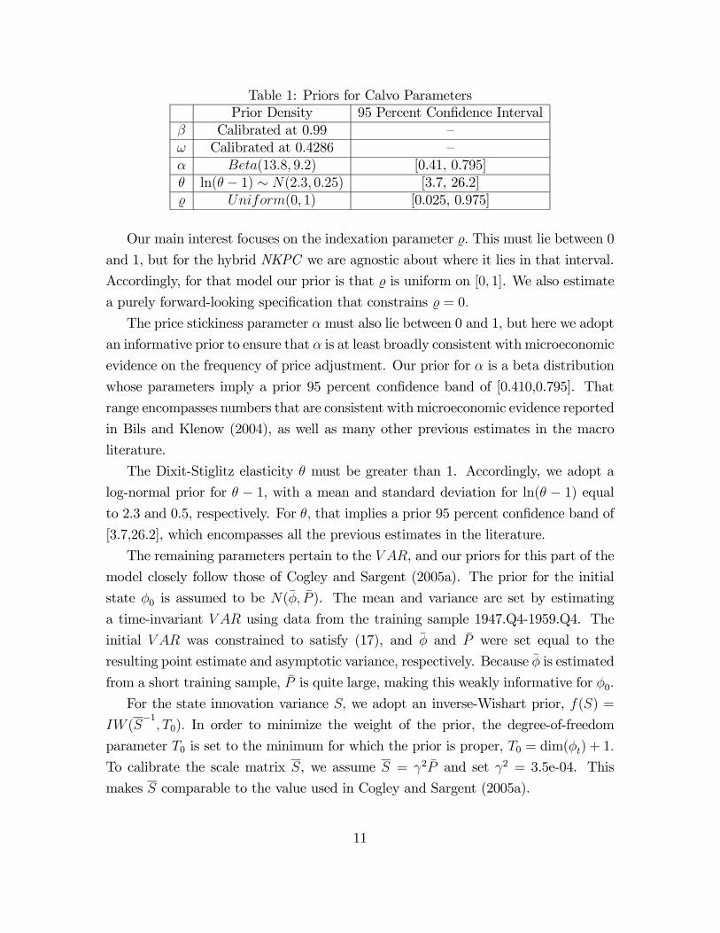
Table 1: Priors for Calvo ParametersPrior Density 95 Percent Confidence Interval

β Calibrated at 0.99 —ω Calibrated at 0.4286 —α Beta(13.8, 9.2) [0.41, 0.795]θ ln(θ − 1) ∼ N(2.3, 0.25) [3.7, 26.2]

Uniform(0, 1) [0.025, 0.975]

Our main interest focuses on the indexation parameter . This must lie between 0

and 1, but for the hybrid NKPC we are agnostic about where it lies in that interval.

Accordingly, for that model our prior is that is uniform on [0, 1]. We also estimate

a purely forward-looking specification that constrains = 0.

The price stickiness parameter α must also lie between 0 and 1, but here we adopt

an informative prior to ensure that α is at least broadly consistent with microeconomic

evidence on the frequency of price adjustment. Our prior for α is a beta distribution

whose parameters imply a prior 95 percent confidence band of [0.410,0.795]. That

range encompasses numbers that are consistent with microeconomic evidence reported

in Bils and Klenow (2004), as well as many other previous estimates in the macro

literature.

The Dixit-Stiglitz elasticity θ must be greater than 1. Accordingly, we adopt a

log-normal prior for θ − 1, with a mean and standard deviation for ln(θ − 1) equalto 2.3 and 0.5, respectively. For θ, that implies a prior 95 percent confidence band of

[3.7,26.2], which encompasses all the previous estimates in the literature.

The remaining parameters pertain to the V AR, and our priors for this part of the

model closely follow those of Cogley and Sargent (2005a). The prior for the initial

state φ0 is assumed to be N(φ, P ). The mean and variance are set by estimating

a time-invariant V AR using data from the training sample 1947.Q4-1959.Q4. The

initial V AR was constrained to satisfy (17), and φ and P were set equal to the

resulting point estimate and asymptotic variance, respectively. Because φ is estimated

from a short training sample, P is quite large, making this weakly informative for φ0.

For the state innovation variance S, we adopt an inverse-Wishart prior, f(S) =

IW (S−1, T0). In order to minimize the weight of the prior, the degree-of-freedom

parameter T0 is set to the minimum for which the prior is proper, T0 = dim(φt) + 1.

To calibrate the scale matrix S, we assume S = γ2P and set γ2 = 3.5e-04. This

makes S comparable to the value used in Cogley and Sargent (2005a).

11

The parameters governing stochastic-volatility priors are set as follows. The prior

for hi0 is log-normal, f(lnhi0) = N(ln hi, 10), where hi is the estimate of the residual

variance of variable i in the initial VAR. A variance of 10 on a natural-log scale

makes this weakly informative for hi0. The prior for b is also normal with a large

variance, f(b) = N(0, 10000). Finally, the prior for σ2i is inverse gamma with a single

degree of freedom, f(σ2i ) = IG(.012/2, 1/2). This also puts a heavy weight on sample

information.

It is worth emphasizing that the priors for S and σ2i — the parameters that govern

the rate of drift in φt and hit — are very weak. In both cases, although the prior

densities are proper, the tails are so fat that they do not possess finite moments.

Thus, our priors about rates of drift are almost entirely agnostic.

5 Estimation results

5.1 Trend Inflation and Persistence of the Inflation Gap

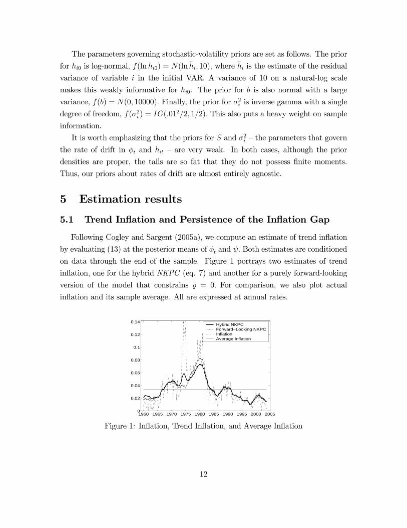
Following Cogley and Sargent (2005a), we compute an estimate of trend inflation

by evaluating (13) at the posterior means of φt and ψ. Both estimates are conditioned

on data through the end of the sample. Figure 1 portrays two estimates of trend

inflation, one for the hybrid NKPC (eq. 7) and another for a purely forward-looking

version of the model that constrains = 0. For comparison, we also plot actual

inflation and its sample average. All are expressed at annual rates.

1960 1965 1970 1975 1980 1985 1990 1995 2000 20050

0.02

0.04

0.06

0.08

0.1

0.12

0.14Hybrid NKPCForward−Looking NKPCInflationAverage Inflation

Figure 1: Inflation, Trend Inflation, and Average Inflation

12

Two features of the graph are relevant for what comes later. The first, of course,

is that trend inflation varies. We estimate that ln πt rose from 2.3 percent in the

early 1960s to 7 or 8 percent just before the Volcker disinflation, then fell to around

2 percent by the end of the sample. A conventional Calvo model seeks to explain

inflation gaps defined in terms of deviations from a constant mean. Since in our case

trend inflation moves over time, we measure the inflation gap as the deviation of

inflation from its time-varying trend, and we seek to model the trend-based inflation

gap.

The second feature concerns the persistence of the inflation gap. Whether the

inflation gap is measured as the deviation from a constant mean or from a time-

varying trend matters a great deal because it affects the degree of persistence. As the

figure illustrates, the mean-based gap is more persistent than trend-based measures.

Notice, for example, the long runs at the beginning, middle, and end of the sample

when inflation does not cross the mean. In contrast, inflation crosses the trend line

much more often, especially after the Volcker disinflation. Purely forward-looking

versions of the Calvo model are often criticized for generating too little persistence

to match mean-based measures of the gap, and a backward-looking element is often

added to accomplish this. Figure 1 makes us wonder whether this ‘excess persistence’

reflects an exaggeration of the persistence in mean-based measures of the gap rather

than a deficiency of persistence in forward-looking models.

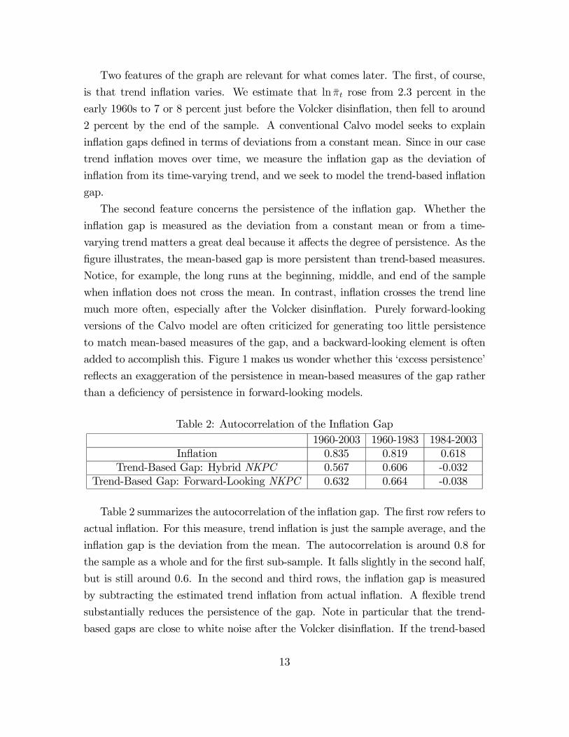
Table 2: Autocorrelation of the Inflation Gap1960-2003 1960-1983 1984-2003

Inflation 0.835 0.819 0.618Trend-Based Gap: Hybrid NKPC 0.567 0.606 -0.032

Trend-Based Gap: Forward-Looking NKPC 0.632 0.664 -0.038

Table 2 summarizes the autocorrelation of the inflation gap. The first row refers to

actual inflation. For this measure, trend inflation is just the sample average, and the

inflation gap is the deviation from the mean. The autocorrelation is around 0.8 for

the sample as a whole and for the first sub-sample. It falls slightly in the second half,

but is still around 0.6. In the second and third rows, the inflation gap is measured

by subtracting the estimated trend inflation from actual inflation. A flexible trend

substantially reduces the persistence of the gap. Note in particular that the trend-

based gaps are close to white noise after the Volcker disinflation. If the trend-based

13

measures are right, for the period after 1983 the NKPC needs to explain only a slight

degree of persistence. A purely forward-looking version may be adequate after all.

5.2 Calvo parameters

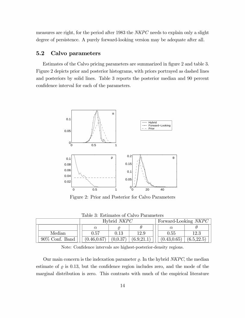
Estimates of the Calvo pricing parameters are summarized in figure 2 and table 3.

Figure 2 depicts prior and posterior histograms, with priors portrayed as dashed lines

and posteriors by solid lines. Table 3 reports the posterior median and 90 percent

confidence interval for each of the parameters.

0 0.5 10

0.05

0.1

α

0 0.5 1

0.02

0.04

0.06

0.08

0.1 ρ

0 20 400

0.05

0.1

0.15

0.2 θ

HybridForward−LookingPrior

Figure 2: Prior and Posterior for Calvo Parameters

Table 3: Estimates of Calvo ParametersHybrid NKPC Forward-Looking NKPC

Median90% Conf. Band

α θ0.57 0.13 12.9

(0.46,0.67) (0,0.37) (6.9,21.1)

α θ0.55 12.3

(0.43,0.65) (6.5,22.5)

Note: Confidence intervals are highest-posterior-density regions.

Our main concern is the indexation parameter . In the hybrid NKPC, the median

estimate of is 0.13, but the confidence region includes zero, and the mode of the

marginal distribution is zero. This contrasts with much of the empirical literature

14

based on mean-based inflation gaps in which is estimated as low as 0.2 and as

high as 1, and is statistically significant. For example, Sbordone (2005) estimates a

of about 0.22 in single equation estimates; Smets and Wouters (2003) in a general

equilibrium model for the euro area estimate a value of approximately 0.5. Giannoni

and Woodford (2003) estimate a value close to 1. Other authors, following Gali and

Gertler (1999), introduce a role for past inflation assuming the presence of rule-of-

thumb firms, instead of through indexation, and also find a significant coefficient on

lagged inflation.

In those models, an important backward-looking component is needed to fit in-

flation persistence, but that is not the case here. From a purely statistical point of

view, a positive coefficient on past inflation may arise in standard Calvo models from

an omitted-variable problem, since the forward-looking terms that are omitted from

standard specifications but which belong to (7) are positively correlated with past

inflation.

The results for the purely forward-looking model are in many respects similar to

those for the hybrid specification. Trend inflation is roughly the same, as are the

estimates of α and θ. Thus, restricting to be zero does not unduly distort other

features of the model.

To compare the hybrid and forward-looking specifications, we calculate a gener-

alization of the Akaike Information Criterion known as the Bayesian Deviance Infor-

mation Criterion (Spiegelhalter, Best, Carlin, and van der Linde, 2002).10 Like the

AIC, the BDIC rewards fit and penalizes model complexity.

Estimates of the BDIC are reported in table 4. The deviance Dev is defined as

-2 times the log likelihood. Dev is the posterior mean of the deviance, and PDev is a

measure of model complexity. The BDIC adds the two together, thus trading off fit

10Bayes factors are often used to compare models, but we prefer the BDIC for two reasons. Thereis much debate among Bayesian statisticians about the reliability of Bayes factors (e.g. see Gelfand1996 or section 6.5 of Gelman, Carlin, Stern and Rubin 2000). In particular, problems connectedwith the Lindley paradox arise when priors are diffuse or weakly informative. That is relevant herebecause our priors are very weakly informative in some dimensions. For example, our priors for Sand σ are proper but do not have moments. Gelfand (1996) recommends against using Bayes factorsin cases like this.A second reason concerns the cost of computing a Bayes factor. Even if we wanted to calculate a

Bayes factor, it would be too costly to do so. In principle, we could apply the methods of Chib (1995)and Chib and Jeliazkov (2001) for Metropolis-within-Gibbs algorithms, but that would involve anauxiliary simulation for each parameter block. Because of the nonlinear cross-equation restrictions,we have a separate block for each φt, and that would entail more than T auxiliary simulations. Wecannot manage that on our workstations.

15

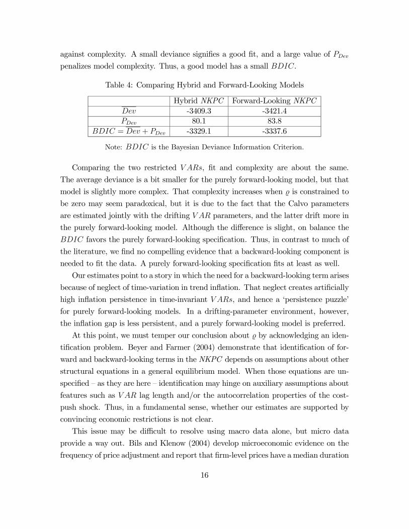
against complexity. A small deviance signifies a good fit, and a large value of PDev

penalizes model complexity. Thus, a good model has a small BDIC.

Table 4: Comparing Hybrid and Forward-Looking Models

Hybrid NKPC Forward-Looking NKPCDev -3409.3 -3421.4PDev 80.1 83.8

BDIC = Dev + PDev -3329.1 -3337.6

Note: BDIC is the Bayesian Deviance Information Criterion.

Comparing the two restricted V ARs, fit and complexity are about the same.

The average deviance is a bit smaller for the purely forward-looking model, but that

model is slightly more complex. That complexity increases when is constrained to

be zero may seem paradoxical, but it is due to the fact that the Calvo parameters

are estimated jointly with the drifting V AR parameters, and the latter drift more in

the purely forward-looking model. Although the difference is slight, on balance the

BDIC favors the purely forward-looking specification. Thus, in contrast to much of

the literature, we find no compelling evidence that a backward-looking component is

needed to fit the data. A purely forward-looking specification fits at least as well.

Our estimates point to a story in which the need for a backward-looking term arises

because of neglect of time-variation in trend inflation. That neglect creates artificially

high inflation persistence in time-invariant V ARs, and hence a ‘persistence puzzle’

for purely forward-looking models. In a drifting-parameter environment, however,

the inflation gap is less persistent, and a purely forward-looking model is preferred.

At this point, we must temper our conclusion about by acknowledging an iden-

tification problem. Beyer and Farmer (2004) demonstrate that identification of for-

ward and backward-looking terms in the NKPC depends on assumptions about other

structural equations in a general equilibrium model. When those equations are un-

specified — as they are here — identification may hinge on auxiliary assumptions about

features such as V AR lag length and/or the autocorrelation properties of the cost-

push shock. Thus, in a fundamental sense, whether our estimates are supported by

convincing economic restrictions is not clear.

This issue may be difficult to resolve using macro data alone, but micro data

provide a way out. Bils and Klenow (2004) develop microeconomic evidence on the

frequency of price adjustment and report that firm-level prices have a median duration

16

of 4.4 months. In a purely forward-looking Calvo model, the waiting time to the next

price change can be approximated as an exponential random variable, and from that

one can calculate the median waiting time as − ln(2)/ ln(α).11 The median estimateof α reported in table 4 implies a half-life of 3.5 months, which is a bit less than Bils

and Klenow’s number. But the confidence region for the half-life ranges from 2.5 to

4.8 months and encompasses their estimate. Therefore our estimated forward-looking

specification is consistent with micro data.

In contrast, backward-looking specifications are more difficult to reconcile with

micro evidence. In a model with indexation, every firm changes price every quarter,

some optimally rebalancing marginal benefit and marginal cost, others mechanically

marking up prices in accordance with the indexation rule. Unless lagged inflation

were exactly zero or the optimal rebalancing happened to confirm the existing price,

no firm would fail to adjust its nominal price. In a world such as that, Bils and Klenow

would not have found that 75 percent of prices remain unchanged each month. We

interpret this as an additional reason to favor a purely forward-looking specification.

Finally, for the forward-looking model, the median estimate of θ implies a steady-

state markup of about 9 percent, with a confidence interval ranging from approxi-

mately 5 to 18 percent. This is in line with many other estimates in the literature.

For instance, Basu (1996) and Basu and Kimball (1997) estimate markups around

10 percent using sectoral data. In general equilibrium models estimated with macro

data, Rotemberg and Woodford (1997) estimate a steady-state markup of 15 percent

(θ ≈ 7.8), Amato and Laubach (2003) find a markup of 19 percent, and Edge et

al. (2003) report a value of 22.7 percent (θ = 5.41). The estimates in Christiano, et

al. (2005) vary from around 6.35 to 20 percent, depending on details of the model

specification.

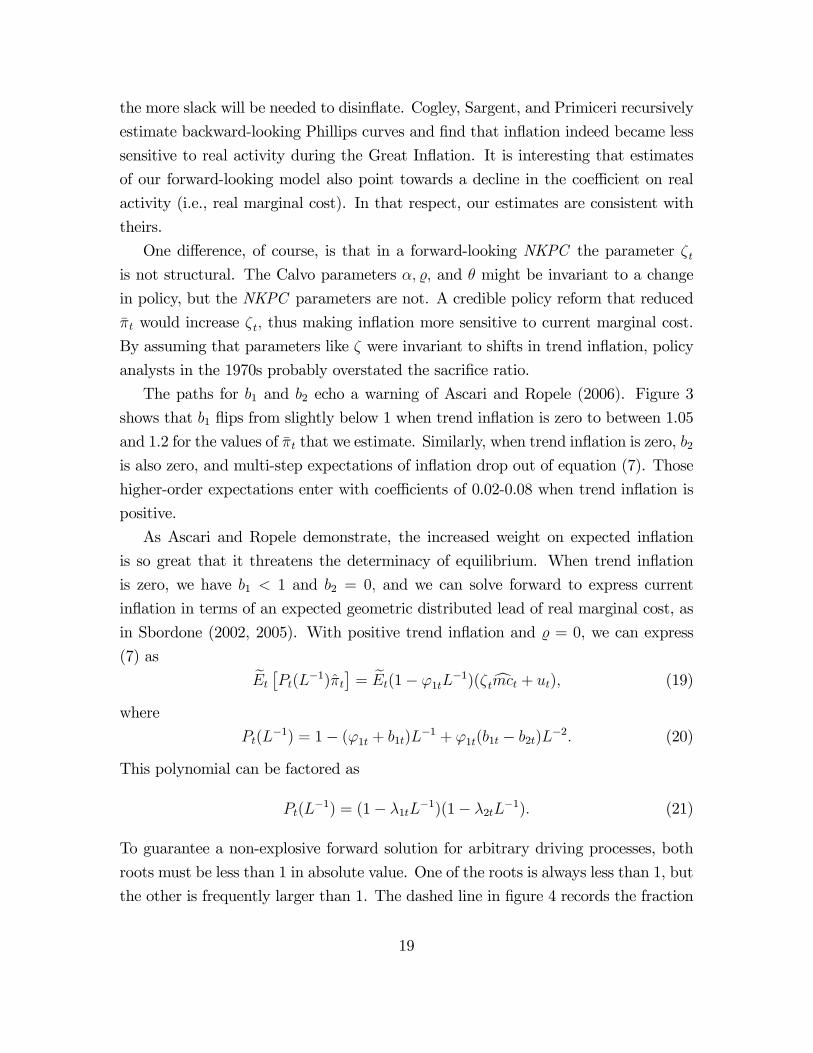
5.3 NKPC Parameters

Next we examine how variation in trend inflation alters the NKPC parameters,

ζ, b1, b2, and ϕ1. These parameters are functions of the Calvo parameters α, , and θ

as well as trend inflation πt, and they vary because πt varies. Figure 3 portrays the

NKPC parameters implied by posterior mean estimates of the Calvo parameters and

11The median waiting time is less than the mean because an exponential distribution has a longupper tail.

17

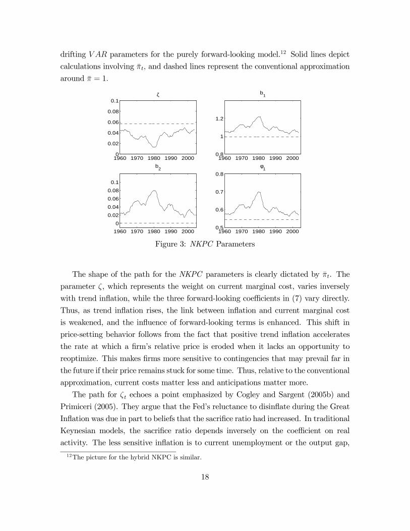
drifting V AR parameters for the purely forward-looking model.12 Solid lines depict

calculations involving πt, and dashed lines represent the conventional approximation

around π = 1.

1960 1970 1980 1990 20000

0.02

0.04

0.06

0.08

0.1ζ

1960 1970 1980 1990 20000.8

1

1.2

b1

1960 1970 1980 1990 2000

0

0.02

0.04

0.06

0.08

0.1

b2

1960 1970 1980 1990 20000.5

0.6

0.7

0.8

φ1

Figure 3: NKPC Parameters

The shape of the path for the NKPC parameters is clearly dictated by πt. The

parameter ζ, which represents the weight on current marginal cost, varies inversely

with trend inflation, while the three forward-looking coefficients in (7) vary directly.

Thus, as trend inflation rises, the link between inflation and current marginal cost

is weakened, and the influence of forward-looking terms is enhanced. This shift in

price-setting behavior follows from the fact that positive trend inflation accelerates

the rate at which a firm’s relative price is eroded when it lacks an opportunity to

reoptimize. This makes firms more sensitive to contingencies that may prevail far in

the future if their price remains stuck for some time. Thus, relative to the conventional

approximation, current costs matter less and anticipations matter more.

The path for ζt echoes a point emphasized by Cogley and Sargent (2005b) and

Primiceri (2005). They argue that the Fed’s reluctance to disinflate during the Great

Inflation was due in part to beliefs that the sacrifice ratio had increased. In traditional

Keynesian models, the sacrifice ratio depends inversely on the coefficient on real

activity. The less sensitive inflation is to current unemployment or the output gap,

12The picture for the hybrid NKPC is similar.

18

the more slack will be needed to disinflate. Cogley, Sargent, and Primiceri recursively

estimate backward-looking Phillips curves and find that inflation indeed became less

sensitive to real activity during the Great Inflation. It is interesting that estimates

of our forward-looking model also point towards a decline in the coefficient on real

activity (i.e., real marginal cost). In that respect, our estimates are consistent with

theirs.

One difference, of course, is that in a forward-looking NKPC the parameter ζtis not structural. The Calvo parameters α, , and θ might be invariant to a change

in policy, but the NKPC parameters are not. A credible policy reform that reduced

πt would increase ζt, thus making inflation more sensitive to current marginal cost.

By assuming that parameters like ζ were invariant to shifts in trend inflation, policy

analysts in the 1970s probably overstated the sacrifice ratio.

The paths for b1 and b2 echo a warning of Ascari and Ropele (2006). Figure 3

shows that b1 flips from slightly below 1 when trend inflation is zero to between 1.05

and 1.2 for the values of πt that we estimate. Similarly, when trend inflation is zero, b2is also zero, and multi-step expectations of inflation drop out of equation (7). Those

higher-order expectations enter with coefficients of 0.02-0.08 when trend inflation is

positive.

As Ascari and Ropele demonstrate, the increased weight on expected inflation

is so great that it threatens the determinacy of equilibrium. When trend inflation

is zero, we have b1 < 1 and b2 = 0, and we can solve forward to express current

inflation in terms of an expected geometric distributed lead of real marginal cost, as

in Sbordone (2002, 2005). With positive trend inflation and = 0, we can express

(7) as eEt

£Pt(L

−1)πt¤= eEt(1− ϕ1tL

−1)(ζtcmct + ut), (19)

where

Pt(L−1) = 1− (ϕ1t + b1t)L

−1 + ϕ1t(b1t − b2t)L−2. (20)

This polynomial can be factored as

Pt(L−1) = (1− λ1tL

−1)(1− λ2tL−1). (21)

To guarantee a non-explosive forward solution for arbitrary driving processes, both

roots must be less than 1 in absolute value. One of the roots is always less than 1, but

the other is frequently larger than 1. The dashed line in figure 4 records the fraction

19

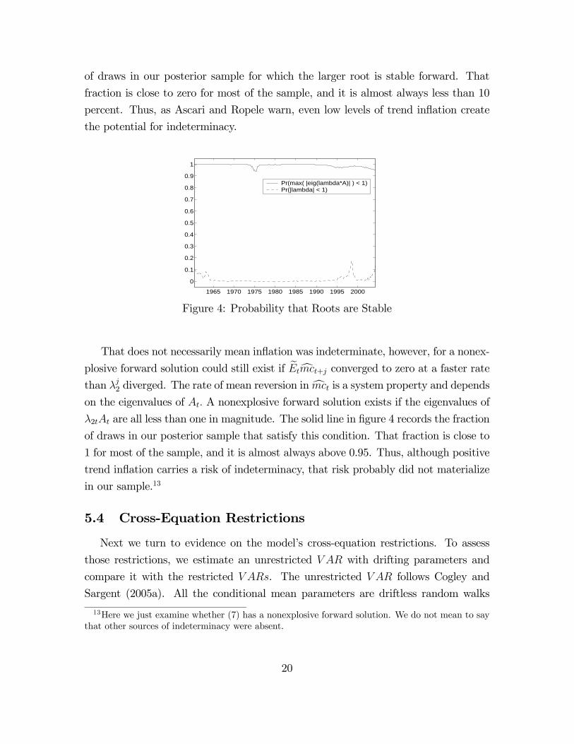
of draws in our posterior sample for which the larger root is stable forward. That

fraction is close to zero for most of the sample, and it is almost always less than 10

percent. Thus, as Ascari and Ropele warn, even low levels of trend inflation create

the potential for indeterminacy.

1965 1970 1975 1980 1985 1990 1995 2000

0

0.1

0.2

0.3

0.4

0.5

0.6

0.7

0.8

0.9

1

Pr(max( |eig(lambda*A)| ) < 1)Pr(|lambda| < 1)

Figure 4: Probability that Roots are Stable

That does not necessarily mean inflation was indeterminate, however, for a nonex-

plosive forward solution could still exist if eEtcmct+j converged to zero at a faster rate

than λj2 diverged. The rate of mean reversion in cmct is a system property and depends

on the eigenvalues of At. A nonexplosive forward solution exists if the eigenvalues of

λ2tAt are all less than one in magnitude. The solid line in figure 4 records the fraction

of draws in our posterior sample that satisfy this condition. That fraction is close to

1 for most of the sample, and it is almost always above 0.95. Thus, although positive

trend inflation carries a risk of indeterminacy, that risk probably did not materialize

in our sample.13

5.4 Cross-Equation Restrictions

Next we turn to evidence on the model’s cross-equation restrictions. To assess

those restrictions, we estimate an unrestricted V AR with drifting parameters and

compare it with the restricted V ARs. The unrestricted V AR follows Cogley and

Sargent (2005a). All the conditional mean parameters are driftless random walks

13Here we just examine whether (7) has a nonexplosive forward solution. We do not mean to saythat other sources of indeterminacy were absent.

20

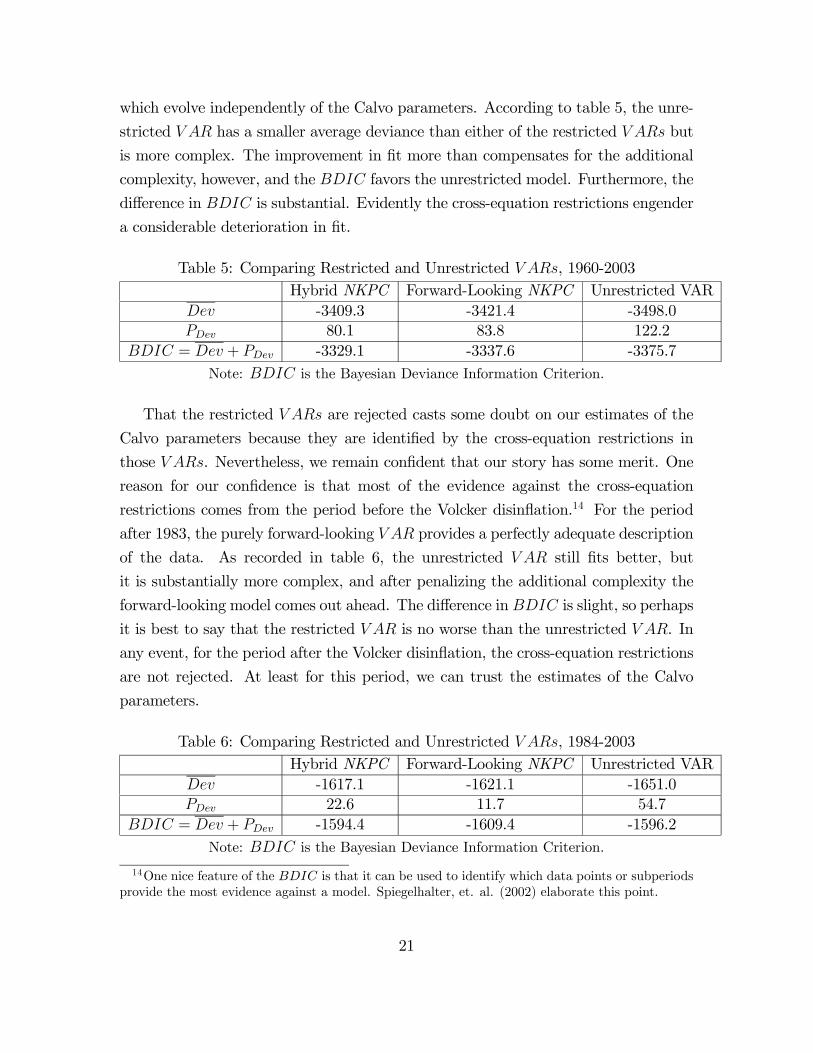
which evolve independently of the Calvo parameters. According to table 5, the unre-

stricted V AR has a smaller average deviance than either of the restricted V ARs but

is more complex. The improvement in fit more than compensates for the additional

complexity, however, and the BDIC favors the unrestricted model. Furthermore, the

difference in BDIC is substantial. Evidently the cross-equation restrictions engender

a considerable deterioration in fit.

Table 5: Comparing Restricted and Unrestricted V ARs, 1960-2003Hybrid NKPC Forward-Looking NKPC Unrestricted VAR

Dev -3409.3 -3421.4 -3498.0PDev 80.1 83.8 122.2

BDIC = Dev + PDev -3329.1 -3337.6 -3375.7Note: BDIC is the Bayesian Deviance Information Criterion.

That the restricted V ARs are rejected casts some doubt on our estimates of the

Calvo parameters because they are identified by the cross-equation restrictions in

those V ARs. Nevertheless, we remain confident that our story has some merit. One

reason for our confidence is that most of the evidence against the cross-equation

restrictions comes from the period before the Volcker disinflation.14 For the period

after 1983, the purely forward-looking V AR provides a perfectly adequate description

of the data. As recorded in table 6, the unrestricted V AR still fits better, but

it is substantially more complex, and after penalizing the additional complexity the

forward-looking model comes out ahead. The difference in BDIC is slight, so perhaps

it is best to say that the restricted V AR is no worse than the unrestricted V AR. In

any event, for the period after the Volcker disinflation, the cross-equation restrictions

are not rejected. At least for this period, we can trust the estimates of the Calvo

parameters.

Table 6: Comparing Restricted and Unrestricted V ARs, 1984-2003Hybrid NKPC Forward-Looking NKPC Unrestricted VAR

Dev -1617.1 -1621.1 -1651.0PDev 22.6 11.7 54.7

BDIC = Dev + PDev -1594.4 -1609.4 -1596.2Note: BDIC is the Bayesian Deviance Information Criterion.

14One nice feature of the BDIC is that it can be used to identify which data points or subperiodsprovide the most evidence against a model. Spiegelhalter, et. al. (2002) elaborate this point.

21

Although the purely forward-looking model generates little inflation persistence,

for the period after the Volcker disinflation there isn’t much inflation-gap persistence

to explain. As noted in table 2, the estimates of the inflation gap shown in figure 1

are close to white noise after 1983. That is why the purely forward-looking model fits

well for this sub-period. The hybrid model still ranks third according to the BDIC,

so there is still little compelling evidence that > 0.

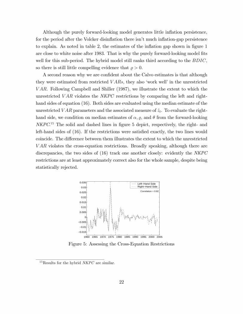
A second reason why we are confident about the Calvo estimates is that although

they were estimated from restricted V ARs, they also ‘work well’ in the unrestricted

V AR. Following Campbell and Shiller (1987), we illustrate the extent to which the

unrestricted V AR violates the NKPC restrictions by comparing the left and right-

hand sides of equation (16). Both sides are evaluated using the median estimate of the

unrestricted V AR parameters and the associated measure of zt. To evaluate the right-

hand side, we condition on median estimates of α, , and θ from the forward-looking

NKPC.15 The solid and dashed lines in figure 5 depict, respectively, the right- and

left-hand sides of (16). If the restrictions were satisfied exactly, the two lines would

coincide. The difference between them illustrates the extent to which the unrestricted

V AR violates the cross-equation restrictions. Broadly speaking, although there are

discrepancies, the two sides of (16) track one another closely: evidently the NKPC

restrictions are at least approximately correct also for the whole sample, despite being

statistically rejected.

1960 1965 1970 1975 1980 1985 1990 1995 2000 2005

−0.015

−0.01

−0.005

0

0.005

0.01

0.015

0.02

0.025

0.03

0.035 Left−Hand SideRight−Hand Side

Correlation = 0.82

Figure 5: Assessing the Cross-Equation Restrictions

15Results for the hybrid NKPC are similar.

22

There are any number of reasons why the cross-equation restrictions might be

violated. Within the model, one possibility is that the ‘nuisance’ terms in (47) that

were omitted from (7) are not nuisances after all. For our estimates, however, the

coefficient b3t in (47) that multiplies those terms is indeed close to zero, so their

omission constitutes only a minor approximation error.

Another possibility is that the Calvo parameters were not constant over the full

sample: in a companion paper, we examine whether the Calvo pricing parameters are

indeed invariant over the full sample.

Finally, another approximation error concerns the assumption that the cost-push

shock ut is white noise. To assess this assumption, we measure ut as the residual in (7)

and then project it onto two lags of πt and cmct.16 The cost-push shock is orthogonal to

lags of real marginal cost, but lags of the inflation gap predict ut with coefficients that

are statistically significant at the 1 percent level. Thus, the white-noise assumption

is rejected. The R2 is just 0.134, however, so the fraction of predictable variation in

ut is not large.

The assumption that ut is unpredictable was used to derive the cross-equation

restrictions. Forecastable movements in ut introduce a wedge in (17) that invalidates

those restrictions. Within the model, the deviations shown in figure 5 can be inter-

preted as a measure of this wedge. Because those discrepancies are relatively small,

it follows that the wedge is also small. Nevertheless, it is not zero, as we assume.

That the parameters of the unrestricted V AR lie close to but not in the subspace

defined by (17) suggests that it would be worthwhile to explore the middle ground

between the restricted and unrestricted models. In principle, this could be done by

extending the work of Del Negro and Schorfheide (2004). For a time-invariant rep-

resentation, Del Negro and Schorfheide show how to elicit a prior on a V AR from

the cross-equation restrictions of a structural model. Their prior is indexed by a

tightness parameter that allows them to strengthen or weaken the influence of the

cross-equation restrictions. In the limit as tightness increases, one can enforce exact

restrictions, as we have done here. By relaxing the tightness, one can enforce approx-

imate restrictions that represent a compromise between restricted and unrestricted

V ARs. To do that for our model, we would have to extend their results to the case

of a drifting-parameter V AR. That extension is nontrivial, and we are working on it.

16Because we want to diagnose the errors in figure 7, we measure ut using the unrestricted V AR.

23

6 Conclusion

Inflation is highly persistent, but much of that persistence is due to shifts in trend

inflation. The inflation gap — i.e., actual minus trend inflation — is less persistent than

inflation itself. The New Keynesian Phillips curve is a model of the inflation gap, but

many previous studies equate inflation with the inflation gap, assuming that trend

inflation is always zero. Because those studies neglect variation in trend inflation,

they attribute all the persistence of inflation to the inflation gap. Matching that

exaggerated degree of persistence requires a backward-looking component which is

typically motivated either as reflecting indexation or rule-of-thumb behavior. Many

NewKeynesian economists are uncomfortable about the backward-looking component

because its microfoundations are less well developed than those of the forward-looking

element.

In this paper, we address whether an extended Calvo model can approximate

inflation dynamics without the introduction of ad hoc backward-looking terms. We

derive a version of the NKPC as an approximate equilibrium condition around a time-

varying inflation trend. Its coefficients are nonlinear combinations of the parameters

describing market structure, the pricing mechanism, and trend inflation. We estimate

the Calvo pricing parameters jointly with the coefficients of a drifting-parameter V AR

that defines trend inflation. Our estimator enforces the cross-equation restrictions

which the NKPC imposes on the V AR.

Among other things, we find that no indexation or backward-looking component is

needed once shifts in trend inflation are taken into account. The posterior distribution

for the backward-looking parameter in a hybrid NKPC has a peak near zero, and a

Bayesian measure of model fit favors a purely forward-looking specification in which

that parameter is constrained to be zero. The purely forward-looking version also

squares better with microeconomic evidence on the frequency of price adjustment.

A number of other papers also report results like ours. Canova (2004), Ireland

(2006) and Milani (2005) all estimate Phillips curve models with shifting inflation

trends, and all report that parameters on backward-looking terms are either zero or

close to zero.17 These papers differ from one another in terms of model specification

and econometric technique, yet they point to a common conclusion. That makes us

17See also Kozicki and Tinsley (2002). They find that shifts in the long-run inflation anchorof agents expectations explain most, but not all of the historical inflation persistence in U.S. andCanada.

24

confident that the result is not driven by idiosyncrasies of our model or estimation

method. The common theme emerging from these papers is that backward-looking

terms in the NKPC become redundant when variation in trend inflation is taken into

account.

Nevertheless, there are a number of ways in which our analysis could be improved.

We assume that the Calvo pricing parameters are invariant to shifts in trend inflation,

which cannot literally be true. In a companion paper, we explore whether that

assumption is a reasonable approximation for the kind of variation in πt seen in

postwar U.S. data.

Another shortcoming concerns the fact that estimates of Calvo pricing parame-

ters come from a restricted V AR which for the sample as a whole fares poorly in

comparison with an unrestricted V AR.18 To remedy that, we are working on an

extension along the lines of Del Negro and Schorfheide (2004), who show how to

estimate structural parameters from approximate rather than exact cross-equation

restrictions.

Perhaps most importantly, we would like to make explicit how agents learn about

trend inflation in real time. In principle, this could be done by adapting the methods

of Sargent, Williams, and Zha (2005). Milani (2005) takes a step in this direction

by estimating a learning model with a univariate perceived law of motion for infla-

tion. It is not clear, however, how that univariate representation squares with the

notion that inflation depends on current and future marginal cost. A learning model

with a multivariate perceived law of motion seems more natural, but that proved to

be computationally intractable. We need to develop a more efficient algorithm for

simulating the posterior, and we leave that to future research.

A Appendix A: Derivation of theNKPC with ran-dom walk trend inflation

In this appendix, we derive a log-linear approximation of the evolution of aggregate

prices and the firms’ first order conditions and explain how to combine them to obtain

the NKPC.18The cross-equation restrictions are not rejected for the period after the Volcker disinflation.

25

A.1 Log-linear approximation of the evolution of aggregateprices

We first divide (6) by Pt to have

1 = (1− α)x1−θt + α(πt−1π−1t )

1−θ. (22)

Then we transform (22) to express it in terms of stationary variables eπt ≡ πt/πt,

gπt = πt/πt−1, and ext = xt/xt :

1 = (1− α)x1−θt ex1−θt + αhπ(1− )(θ−1)t

i ¡gπt¢− (1−θ) eπ (1−θ)

t−1 eπ−(1−θ)t . (23)

In steady state, this defines a function xt = x (πt):

xt =

"1− απ

(1− )(θ−1)t

1− α

# 11−θ

. (24)

Defining hat variables bxt ≡ ln (ext) and bπt ≡ ln (eπt) , the log-linear approximation of(23) around its steady state is:

0 ' (1− α)x1−θt bxt − αhπ(1− )(θ−1)t

i ¡bπt − ¡bπt−1 − bgπt ¢¢ , (25)

which, substituting (1− α)x1−θt from (24), becomes

0 'h1− απ

(1− )(θ−1)t

i bxt − αhπ(1− )(θ−1)t

i ¡bπt − ¡bπt−1 − bgπt ¢¢ . (26)

This expression gives a solution for bxt as a function of bπt, bπt−1 and bgπt :bxt = απ

(1− )(θ−1)t

1− απ(1− )(θ−1)t

£bπt − ¡bπt−1 − bgπt ¢¤ . (27)

A.2 Log-linear approximation of firm’s FOC

The relation between marginal cost at t+ j of the firm that changes price at t and

average marginal cost at t+ j is

MCt+j,t =MCt+j

µXΨtj

Pt+j

¶−θω=MCt+jX

−θωt Ψ−θωtj P θω

t+j, (28)

where ω is the elasticity of firm’s marginal cost to its own output. Substituting (28)

in the first-order conditions (eq. 5), we have

eEt

X∞j=0

αjQt,t+jYt+jPθt+jΨ

1−θtj

µX(1+ωθ)t − θ

θ − 1MCt+jΨ−(1+θω)tj P θω

t+j

¶= 0, (29)

26

which implies

X(1+ωθ)t =

θ

θ − 1eEt

P∞j=0 α

jqt,t+jYt+jPθ(1+ω)−1t+j Ψ

−θ(1+ω)tj MCt+jeEt

P∞j=0 α

jqt,t+jYt+jPθ−1t+j Ψ

1−θtj

≡ Ct

Dt. (30)

Here we express the discount factor in real terms as qt,t+j = Qt,t+jPt+j/Pt, and we

define qt,t+j =Yj−1

k=0qt+k,t+k+1. Using the definition of Ψtj in (3), we can express C

and D recursively as

Ct =θ

θ − 1YtPθ(1+ω)−1t MCt + eEt

hα qt,t+1π

− θ(1+ω)t Ct+1

i(31)

Dt = YtPθ−1t + eEt

hα qt,t+1π

(1−θ)t Dt+1

i. (32)

After appropriately ‘deflating’ (31) and (32), we obtain

eCt ≡ Ct

YtPθ(1+ω)t

=θ

θ − 1mct + eEt

hα qt,t+1g

yt+1 (πt+1)

θ(1+ω) π− θ(1+ω)t

eCt+1

i(33)

eDt ≡ Dt

YtPθ−1t

= 1 + eEt

hα qt,t+1g

yt+1 (πt+1)

θ−1 π (1−θ)t

eDt+1

i, (34)

where mct ≡MCt/Pt. Note that the ratio of (33) and (34) gives:

eCteDt

=Ct

Dt

YtPθ−1t

YtPθ(1+ω)t

=Ct

Dt

1

P(1+θω)t

=

µXt

Pt

¶1+θω≡ x1+θωt . (35)

Evaluating (33) and (34) at the steady state, we solve for

Ct =θ

θ−1mct

1− α qgy (πt)θ(1+ω)(1− )

, (36)

Dt =1

1− α qgy (πt)(θ−1)(1− )

, (37)

so that

x1+θωt =Ct

Dt

=

"1− α qgy (πt)

(θ−1)(1− )

1− α qgy (πt)θ(1+ω)(1− )

#θ

θ − 1mct. (38)

Note that we assume the following two inequalities to hold:

α qgy (πt)θ(1+ω)(1− ) < 1, (39)

α qgy (πt)(θ−1)(1− ) < 1. (40)

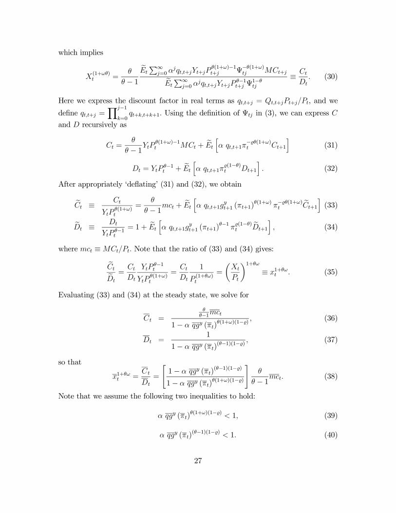
27

We can solve (36), (37), (38) for functions mc(πt), C(πt), D(πt), while (24) gives a

function x(πt).

To derive a log-linear approximation of (35), we define bCt = ln( eCt/Ct) and bDt =

ln( eDt/Dt), and derive

bCt = ϕ3tcmct + ϕ2t eEt[bqt,t+1 + bgyt+1 + θ (1 + ω)¡bπt+1 − bπt + bgπt+1¢+ bgCt+1]

+ϕ2t eEtbCt+1, (41)

bDt = ϕ1t eEt[bqt,t+1 + bgyt+1 + (θ − 1) ¡bπt+1 − bπt + bgπt+1¢+ bgDt+1] + ϕ1t eEtbDt+1. (42)

The hat variables are defined as cmct = ln(mct/mct), bqt,t+1 = ln(qt/q), bgπt+1 =ln(πt+1/πt), bgCt+1 = ln(Ct+1/Ct), and bgDt+1 = ln(Dt+1/Dt). The symbols ϕ1t, ϕ2t and

ϕ3t are defined as

ϕ1t = αeβπ(1− )(θ−1)t ,

ϕ2t = αeβπθ(1+ω)(1− )t , (43)

ϕ3t = 1− α q gy πθt = 1− ϕ2t,

where eβ ≡ qgy. From (35), we then have

(1 + θω) bxt = bCt − bDt, (44)

from which we can solve for bπt using (27)bπt = ¡bπt−1 − bgπt ¢+ 1− απ

(1− )(θ−1)t

απ(1− )(θ−1)t

bxt. (45)

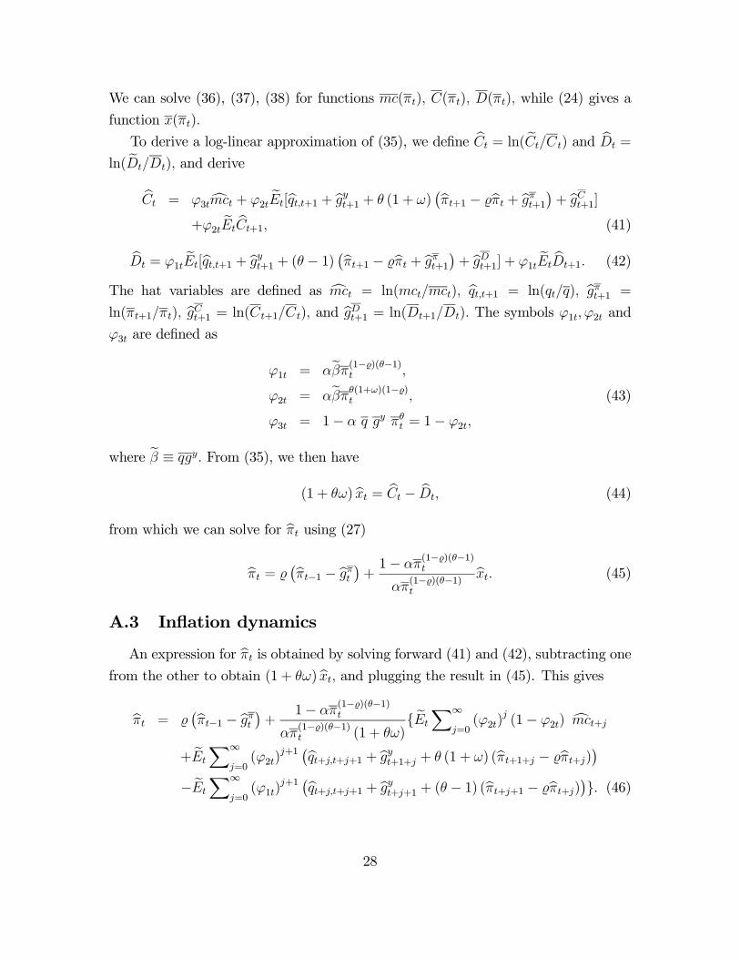
A.3 Inflation dynamics

An expression for bπt is obtained by solving forward (41) and (42), subtracting onefrom the other to obtain (1 + θω) bxt, and plugging the result in (45). This gives

bπt =¡bπt−1 − bgπt ¢+ 1− απ

(1− )(θ−1)t

απ(1− )(θ−1)t (1 + θω)

{ eEt

X∞j=0(ϕ2t)

j (1− ϕ2t) cmct+j

+ eEt

X∞j=0(ϕ2t)

j+1 ¡bqt+j,t+j+1 + bgyt+1+j + θ (1 + ω) (bπt+1+j − bπt+j)¢− eEt

X∞j=0(ϕ1t)

j+1 ¡bqt+j,t+j+1 + bgyt+j+1 + (θ − 1) (bπt+j+1 − bπt+j)¢}. (46)

28

Here we use the fact that eEtbgCt+1 = eEtbgDt+1 = 0, and eEtbgπt+j = 0 for j ≥ 1. When

we solve forward, we also invoke an anticipated-utility approximation. That approx-

imation treats drifting parameters as if they would remain constant at their current

value when making multi-step forecasts.

Finally, to obtain equation (7), we evaluate (46) at t + 1, multiply it by ϕ2t+1,

take expectations, and subtract the resulting expression from (46). The generalized

NKPC is

bπt = et ¡bπt−1 − bgπt ¢+ ζt cmct + b1t eEtbπt+1 + b2t eEt

X∞j=2

ϕj−11t bπt+j (47)

+b3t eEt

X∞j=0

ϕj1t

£bqt+j,t+j+1 + bgyt+j+1¤+ ut,

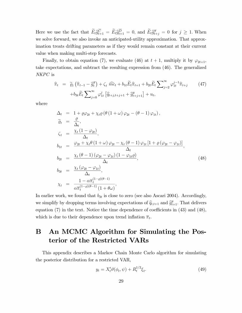
where

∆t = 1 + ϕ2t + χt (θ (1 + ω)ϕ2t − (θ − 1)ϕ1t) ,et =∆t

,

ζt =χt (1− ϕ2t)

∆t,

b1t =ϕ2t + χtθ (1 + ω)ϕ2t − χt (θ − 1)ϕ1t [1 + (ϕ2t − ϕ1t)]

∆t,

b2t =χt (θ − 1) (ϕ2t − ϕ1t) (1− ϕ1t )

∆t, (48)

b3t =χt (ϕ2t − ϕ1t)

∆t,

χt =1− απ

(1− )(θ−1)t

απ(1− )(θ−1)t (1 + θω)

,

In earlier work, we found that b3t is close to zero (see also Ascari 2004). Accordingly,

we simplify by dropping terms involving expectations of bqt,t+1 and bgyt+1. That deliversequation (7) in the text. Notice the time dependence of coefficients in (43) and (48),

which is due to their dependence upon trend inflation πt.

B An MCMC Algorithm for Simulating the Pos-terior of the Restricted VARs

This appendix describes a Markov Chain Monte Carlo algorithm for simulating

the posterior distribution for a restricted VAR,

yt = X 0tϑ(φt, ψ) +R

1/2t ξt. (49)

29

The posterior is

f(ψ, φT , S, σ, β21, HT |Y T ), (50)

where ψ are the Calvo parameters, Y T = [y01, ..., y0T ]

0, φT = [φ01, ..., φ0T ]

0, and HT =

[diag(H1)0, ..., diag(HT )

0]0 represent histories of the data, the drifting V AR parame-

ters, and the stochastic volatilities, respectively. The matrix S represents the variance

of innovations to φt, the vector σ = (σ1, σ2) lists the standard deviations of the inno-

vations to ln(hit), and β21 is the residual covariance parameter (i.e., the (2, 1) element

of the matrix B).

We group the parameters into 6 blocks and design a Metropolis-within-Gibbs

algorithm for simulating the posterior. The blocks are

• φT |ψ, S, σ, β21, HT , Y T

• ψ|φT , S, σ, β21, HT , Y T

• S|ψ, φT , σ, β21,HT , Y T

• HT |ψ, φT , S, σ, β21, Y T

• β21|ψ, φT , S, σ,HT , Y T

• σ|ψ, φT , S, σ, β21,HT , Y T

The simulators for the last four are identical to those in Cogley and Sargent (2005a);

interested readers should consult their appendices. Here we concentrate on the blocks

for φt and ψ.

B.1 φ-Block

Consider first the distribution of φT conditional on the data and other parame-

ters. The problem here involves simulating a posterior for drifting V AR parameters

that are subject to nonlinear cross-equation restrictions. Following Carlin, Polson,

and Stoffer (1992), Cogley (2005) develops a Metropolis-Hastings algorithm for this

problem. We adapt that algorithm.

From Bayes’s theorem, the conditional kernel for φT can be expressed as the

product of a conditional likelihood function and a conditional prior for φT ,

f(φT |ψ, S, σ, β21,HT , Y T ) ∝ f(Y T |φT , ψ, S, σ, β21,HT )f(φT |ψ, S, σ, β21,HT ). (51)

30

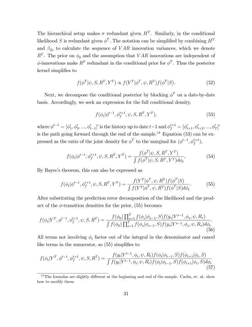
The hierarchical setup makes σ redundant given HT . Similarly, in the conditional

likelihood S is redundant given φT . The notation can be simplified by combining HT

and β21 to calculate the sequence of V AR innovation variances, which we denote

RT . The prior on φ0 and the assumption that V AR innovations are independent of

φ-innovations make RT redundant in the conditional prior for φT . Thus the posterior

kernel simplifies to

f(φT |ψ, S,RT , Y T ) ∝ f(Y T |φT , ψ,RT )f(φT |S). (52)

Next, we decompose the conditional posterior by blocking φT on a date-by-date

basis. Accordingly, we seek an expression for the full conditional density,

f(φt|φt−1, φt+1f , ψ, S,RT , Y T ), (53)

where φt−1 = [φ01, φ02, ..., φ

0t−1]

0 is the history up to date t−1 and φt+1f = [φ0t+1, φ0t+2, ..., φ

0T ]0

is the path going forward through the end of the sample.19 Equation (53) can be ex-

pressed as the ratio of the joint density for φT to the marginal for (φt−1, φt+1f ),

f(φt|φt−1, φt+1f , ψ, S,RT , Y T ) =f(φT |ψ, S,RT , Y T )Rf(φT |ψ, S,RT , Y T )dφt

, (54)

By Bayes’s theorem, this can also be expressed as

f(φt|φt−1, φt+1f , ψ, S,RT , Y T ) =f(Y T |φT , ψ,RT )f(φT |S)Rf(Y T |φT , ψ,RT )f(φT |S)dφt

. (55)

After substituting the prediction error decomposition of the likelihood and the prod-

uct of the φ-transition densities for the prior, (55) becomes

f(φt|Y T , φt−1, φt+1f , ψ, S,RT ) =f(φ0)

QTs=1 f(φs|φs−1, S)f(ys|Y s−1, φs, ψ,Rs)R

f(φ0)QT

s=1 f(φs|φs−1, S)f(ys|Y s−1, φs, ψ,Rs)dφt.

(56)

All terms not involving φt factor out of the integral in the denominator and cancel

like terms in the numerator, so (55) simplifies to

f(φt|Y T , φt−1, φt+1f , ψ, S,RT ) =f(yt|Y t−1, φt, ψ,Rt)f(φt|φt−1, S)f(φt+1|φt, S)Rf(yt|Y t−1, φt, ψ,Rt)f(φt|φt−1, S)f(φt+1|φt, S)dφt

(57)

19The formulas are slightly different at the beginning and end of the sample. Carlin, et. al. showhow to modify them.

31

Because the likelihood function is nonlinear in φt, we apply a Metropolis-Hastings

step to the conditional kernel in the numerator. Our proposal density is the product

of the transition densities,

q(φt|φt−1, φt+1, S) ∝ f(φt|φt−1, S)f(φt+1|φt, S). (58)

By taking the log of q(·) and completing the square, one can show that the proposalis normal with mean µt = (1/2)(φt−1 + φt+1) and variance Vt = (1/2)S.

The acceptance probability at scan j, denoted λj, depends on the current proposal,

φt, and the previous draw, φj−1t :

λ(φt, φj−1t ) = min

Ã1,

f(yt|Y t−1, φt, ψ,Rt)q(φt|φt−1, φt+1, S)f(yt|Y t−1, φj−1t , ψ,Rt)q(φ

j−1t |φt−1, φt+1, S)

q(φj−1t |φt−1, φt+1, S)q(φt|φt−1, φt+1, S)

!,

= min

Ã1,

f(yt|Y t−1, φt, ψ,Rt)

f(yt|Y t−1, φj−1t , ψ,Rt)

!. (59)

If the proposal is accepted, the chain advances to φjt = φt. Otherwise φjt is set equal

to φj−1t .

The only remaining question concerns how to evaluate the likelihood function for

the restricted VAR. The innovations are conditionally normal with mean X 0tϑ(φt, ψ)

and variance Rt, so we just need to calculate the restricted parameters ϑ(φt, ψ).

The free parameters φt include the V AR intercepts along with the autoregressive

parameters of the share equation. According to equations (17) and (48), φt and

ψ pin down the autoregressive parameters of the inflation equation via the model’s

cross-equation restrictions. These equations are nonlinear, so for given values of φtand ψ we solve numerically for the inflation parameters. For some proposals our

nonlinear equation solver fails to converge. We interpret nonconvergence as a sign

that φt is unlikely under the NKPC, and we set λj = 0, φjt = φj−1t when that happens.

B.2 ψ-Block

This block is a nonlinear least squares problem with time-invariant parameters,

and we use a random-walk Metropolis chain to simulate its posterior. Proposals

evolve as

ψj = ψj−1 + cψV1/2ψ εj, (60)

32

where εj is standard normal, Vψ is a guess about the posterior variance of ψ, and cψ

is an arbitrary scalar chosen to achieve a desirable acceptance rate. We initialize the

proposal chain using output from the two-step simulation described in Cogley and

Sbordone (2005). The initial value of the chain ψ0 is the mean of that distribution,

and Vψ is the variance. After some experimentation, we set cψ = 0.1.

Because this is a random-walk chain with symmetric increments, the acceptance

probability is

λ(ψ∗j) = min

"1,

f(ψj|Y T , ·)f(ψj−1|Y T , ·)

#, (61)

where f(ψ|Y T , ·) is the conditional posterior,

f(ψ|Y T , ·) ∝ f(Y T |φT , ψ,RT )f(ψ). (62)

Notice that proposals which violate any of the bounds have prior probability zero and

thus have an acceptance probability of zero. The log-likelihood function is

log f(Y T |ψ, ·) = −12

Xtlog |Rt| + wt

0R−1t wt, (63)

where wt = yt−X 0tϑ(φt, ψ). For each guess of ψ and φt, we solve (17) numerically to

calculate ϑ(φt, ψ). Otherwise this block is standard.

B.3 Number of draws and convergence

The results reported in the text are based on 200,000 draws from the Markov chain.

The first 100,000 were discarded to allow for convergence. To economize on storage

requirements, we saved every 10th draw and discarded the rest. Convergence was

diagnosed by inspecting recursive mean plots. It is good practice also to inspect the

results of parallel chains that started from different initial conditions. Regrettably,

that was not practical in this case because of the high computational of each chain.

References

[1] Adolfson, Malin; Laseen, Stefan; Linde’, Jasper and Villani, Mattias. “Bayesian

Estimation of an Open Economy DSGE Model with Incomplete Pass-Through.”

Working paper n. 179, Sveridges Riksbank, 2005.

33

[2] Altig, David; Christiano, Lawrence J.; Eichenbaum, Martin and Jesper Linde’.

“Firm-Specific Capital, Nominal Rigidities and the Business Cycle.” Unpub-

lished, 2004.

[3] Amato, Jeffrey and Laubach, Thomas. “Estimation and control of an

optimization-based model with sticky prices and wages.” Journal of Economic

Dynamics and Control, 2003, 27 (7), pp. 1181-1215.

[4] Ascari, Guido. “Staggered prices and trend inflation: some nuisances.” Review

of Economic Dynamics, 2004, 7 (3), pp. 642-667.

[5] Ascari, Guido and Ropele, Tiziano. “Optimal Monetary Policy under Low Trend

Inflation.” Unpublished, 2006.

[6] Bakhshi, Hasan; Burriel-Llombart, Pablo; Khan, Hashmat and Rudolf, Barbara.

“Endogenous price stickiness, trend inflation and the new Keynesian Phillips

curve.” Bank of England working paper no. 191, 2003.

[7] Basu, Susanto. “Procyclical productivity: increasing returns or cyclical utiliza-

tion?”, Quarterly Journal of Economics, 1996, 111 (3), pp. 719-751.

[8] Basu, Susanto and Kimball, Miles. “Cyclical productivity with unobserved input

variation.” NBER working paper no. 5915, 1997.

[9] Beyer, Andreas. and Farmer, Roger E.A. “On the indeterminacy of new Keyne-

sian economics.” European Central Bank, working paper 323, 2004.

[10] Bils, Mark and Klenow, Peter J. “Some evidence on the importance of sticky

prices.” Journal of Political Economy, 2004, 112 (5), pp. 947-985.

[11] Calvo, Guillermo. “Staggered prices in a utility-maximizing framework.” Journal

of Monetary Economics, 1983, 12 (3), pp. 383-398.

[12] Campbell, John Y. and Shiller, Robert J. “Cointegration and tests of present

value models.” Journal of Political Economy, 1987, 95 (5), pp. 1062-1088.

[13] Canova, Fabio. “Monetary Policy and the evolution of the U.S. economy 1948-

2002.” Unpublished, 2004.

34

[14] Carlin, B.P.; Polson, N.G. and Stoffer, D.S. “A Monte Carlo Approach to Non-

normal and Nonlinear State-Space Modeling.” Journal of the American Statisti-

cal Association, 1992, 87 (418), pp. 493-500.

[15] Chib, Siddhartha. “Marginal Likelihood From the Gibbs Output,” Journal of

the American Statistical Association, 1995, 90 (432), pp. 1313-1321.

[16] Chib, Siddhartha and Jeliazkov, Ivan. “Marginal Likelihood from the Metropolis-

Hastings Output.” Journal of the American Statistical Association, 2001,

96 (453), pp. 270-281.

[17] Christiano, Lawrence; Eichenbaum, Martin and Evans, Charles. “Nominal rigidi-

ties and the dynamic effects of a shock to monetary policy.” Journal of Political

Economy, 2005, 113(1), pp. 1-45.

[18] Cogley, Timothy. “Changing Beliefs and the Term Structure of Interest Rates:

Cross-Equations Restrictions with Drifting Parameters.” Review of Economic

Dynamics, 2005, 8(2), pp. 420-451.

[19] Cogley, Timothy and Sargent, Thomas J. “Drifts and Volatilities: Monetary

Policies and Outcomes in the Post WWII U.S.” Review of Economic Dynamics,

2005a, 8 (2), pp. 262-302.

[20] –––- “The Conquest of U.S. Inflation: Learning and Robustness to Model

Uncertainty.” Review of Economic Dynamics, 2005b, 8 (2), pp. 528-563.

[21] –––- “Anticipated Utility and Rational Expectations as Approximations of

Bayesian Decision Making.” Unpublished, 2006.

[22] Cogley, Timothy and Sbordone, Argia M. “A Search for a Structural Phillips

Curve.” Staff Report # 203, Federal Reserve Bank of New York, 2005.

[23] Del Negro, Marco and Schorfheide, Frank. “Priors from general equilibriummod-

els for VARs.” International Economic Review, 2004, 45 (2), pp. 643.673.

[24] Economic Report of the President 2004. United States Government Printing

Office, Washington DC.

35

[25] Edge, Rochelle M.; Laubach, Thomas and Williams, John C. “The response

of wages and prices to technology shocks.” Federal Reserve Board Finance and

Economics Discussion Series 2004-65.

[26] Eichenbaum, Martin and Fisher, Jonas. “Evaluating the Calvo Model of Sticky-

Prices.”, NBER working paper n. 10617, July 2004.

[27] Evans, George W. and Honkapohja, Seppo. Learning and Expectations in Macro-

economics, Princeton: Princeton University Press, 2001.

[28] Fuhrer, Jeff and Moore, George. “Inflation Persistence.” Quarterly Journal of

Economics, 1995, 110 (1), pp. 127-159.

[29] Gali, Jordi and Gertler, Mark. “Inflation dynamics: A structural econometric

analysis.” Journal of Monetary Economics, 1999, 44 (2), pp. 195-222.

[30] Gelfand, Alan E. “Model determination using sampling-based methods.” InW.R.

Gilks, S. Richardson, and D.J. Spiegelhalter, eds., Markov Chain Monte Carlo

in Practice, London: Chapman and Hall, 1996.

[31] Gelman, Andrew; Carlin, John B.; Stern, Hal S. and Rubin, Donald B. Bayesian

Data Analysis, London: Chapman and Hall, 2000.

[32] Giannoni, Marc and Woodford, Michael. “Optimal inflation targeting rules.” In

B. Bernanke and M. Woodford, eds. Inflation Targeting, Chicago: University of

Chicago Press, 2003.

[33] Ireland, Peter N. “Changes in the Federal Reserve’s Inflation Target: Causes and

Consequences.” Unpublished, 2006.

[34] Kiley, Michael. “Is Moderate-To-High Inflation Inherently Unstable?” Federal

Reserve Board Finance and Economics Discussion Series n. 2004-43.

[35] Kozicki, Sharon and Tinsley, Peter A. “Alternative Sources of the Lag Dynam-

ics of Inflation.” In Price Adjustment and Monetary Policy, Bank of Canada

Conference Proceedings, 2002, pp. 3-47.

[36] Kreps, David M. “Anticipated Utility and Dynamic Choice.” In Frontiers of

Research in Economic Theory, edited by Jacobs, D.P.; Kalai, E. and Kamien,

M., Cambidge: Cambridge University Press, 1997.

36

[37] Matheron, Julien. ““Firm-Specific Labor vs. Firm-Specific Capital: Implications

for the Euro Data New Phillips Curve.” unpublished, 2005.

[38] Milani, Fabio. “A Bayesian DSGE model with infinite horizon learning: do me-

chanical sources of persistence become superfluous?” Unpublished, 2005.

[39] Primiceri, Giorgio E. “Why Inflation Rose and Fell: Policy-makers’ Beliefs and

U.S. Postwar Stabilization Policy, Quarterly Journal of Economics (forthcom-

ing).

[40] Rotemberg, Julio J. and Woodford, Michael. “An Optimization-based economet-

ric framework for the evaluation of monetary policy.” In B. Bernanke and J.J.

Rotemberg, eds, NBER Macroeconomics Annual, MIT press, Cambridge, 1997,

12, pp. 297-346.

[41] Sahuc, Jean-Guillaume. “Partial indexation, trend inflation, and the hybrid

Phillips curve.” Economics Letters, 2006, 90 (1), pp. 42-50.

[42] Sargent, Thomas J.; Williams, Noah and Zha, Tao. “Shocks and government

beliefs: the rise and fall of American inflation.” American Economic Review

(forthcoming).

[43] Sbordone, Argia M. “Price and unit labor costs: a new test of price stickiness.”

Journal of Monetary Economics, 2002, 49 (2), pp. 265-292.

[44] ––––––— “Do expected future marginal costs drive inflation dynamics?”

Journal of Monetary Economics, 2005, 52 (6), pp. 1183-1197.

[45] Schorfheide, Frank. “Learning and monetary policy shifts.” Review of Economic

Dynamics, 2005, 8(2), pp. 392-419.

[46] Smets, Frank and Wouters, Ralph. “An Estimated Dynamic Stochastic Gen-

eral Equilibrium Model of the Euro Area.” Journal of the European Economic

Association, 2003, 1 (5), pp. 1123-1175.

[47] –––––––- “Comparing shocks and frictions in US and euro area business

cycles: a Bayesian DSGE Approach.” Journal of Applied Econometrics, 2005,

20 (2), pp. 161-183.

37

[48] Spiegelhalter, David.J.; Best, Nicola G.; Carlin, Bradley P. and van der Linde,

Angelika. “Bayesian measures of model complexity and fit.” (with discussion)

Journal of the Royal Statistical Society B, 2002, 64, pp. 583-640.

[49] Stock, James H. and Watson, Mark W. “Why Has U.S. Inflation Become Harder

to Forecast?” NBER working paper n. 12324, June 2006.

[50] Woodford, Michael. “Firm-Specific Capital and the New Keynesian Phillips

Curve.” International Journal of Central Banking, 2005, 1(2), pp. 1-46.

38