Understanding inflation persistence: a comparison of different models

ISSN 1561081-0

9 7 7 1 5 6 1 0 8 1 0 0 5

WORKING PAPER SER IESNO 672 / SEPTEMBER 2006

A COMPARISON OF DIFFERENT MODELS

and Engin Karaby Huw Dixon

UNDERSTANDINGINFLATION PERSISTENCE

In 2006 all ECB publications

feature a motif taken

from the €5 banknote.

WORK ING PAPER SER IE SNO 672 / S EPTEMBER 2006

This paper can be downloaded without charge from http://www.ecb.int or from the Social Science Research Network

electronic library at http://ssrn.com/abstract_id=926344

comments. Part of this paper was completed while Engin Kara was visiting the Monetary Policy Strategy Division at the European Central Bank and he thanks them for their hospitality. Faults remain our own.

2 Economics Department, University of York, Heslington, York, YO10 5DD, United Kingdom; e-mail: [email protected] University of York; e-mail: [email protected]

A COMPARISON OF DIFFERENT MODELS 1

2

and Engin Kara 3

by Huw Dixon

1 We would like to thank Neil Rankin, Filippo Altissimo, Frank Smets and seminar participants at Cardiff and Manchester for their

UNDERSTANDINGINFLATION PERSISTENCE

© European Central Bank, 2006

AddressKaiserstrasse 2960311 Frankfurt am Main, Germany

Postal addressPostfach 16 03 1960066 Frankfurt am Main, Germany

Telephone+49 69 1344 0

Internethttp://www.ecb.int

Fax+49 69 1344 6000

Telex411 144 ecb d

All rights reserved.

Any reproduction, publication andreprint in the form of a differentpublication, whether printed orproduced electronically, in whole or inpart, is permitted only with the explicitwritten authorisation of the ECB or theauthor(s).

The views expressed in this paper do notnecessarily reflect those of the EuropeanCentral Bank.

The statement of purpose for the ECBWorking Paper Series is available fromthe ECB website, http://www.ecb.int.

ISSN 1561-0810 (print)ISSN 1725-2806 (online)

3ECB

Working Paper Series No 672September 2006

CONTENTSAbstract 4

Non-technical summary 5

1 Introduction 7

2 The model 11

2.1 Structure of the economy 11

2.2 The log-linearised economy 12

2.3 Wage setting rules 13

2.4 The choice of parameters 14

3 Inflation persistence in a generalised Tayloreconomy (GTE) 15

3.1 Generalised Taylor economy (GTE) 16

3.1.1 Calvo-GTE 17

18

4 Generalised Fischer economy (GFE) 18

4.1 Simple Fischer economy 19

4.2 Mankiw and Reis’s sticky information(SI) model 20

5 Hybrid Phillips curve models 21

5.1 Fuhrer and Moore’s (1995) inflationpersistence model 21

5.2 Calvo with full indexation:Woodford (2003) 22

5.3 GTE with full indexation 23

5.4 Kiley (2005): Calvo with indexationbased on a moving average 24

6 What is the effect of γ? 24

7 Output and inflation 26

8 Conclusion 27

References 30

Appendix 33

Tables and figures 41

European Central Bank Working Paper Series 51

3.1.2 Bils-Klenow distribution: BK – GTE

Abstract

This paper adopts the Impulse-Response methodology to under-stand in ation persistence. It has often been argued that existingmodels of pricing fail to explain the persistence that we observe. Weadopt a common general framework which allows for an explicit mod-elling of the distribution of contract lengths and for di�erent types ofprice setting. In particular, we �nd that allowing for a distributionof contract lengths can yield a more plausible explanation of in ationpersistence than indexation.

Keywords: DGE models, in ation, persistence, price-setting.JEL: E17, E3.

4ECBWorking Paper Series No 672September 2006

Non-Technical Summary

The persistence of in ation is a central issue both for economic policymakers and for theorists. For policy makers the issue is how far they shouldlook forward and how rapidly their policy actions take e�ect. For theorists,the issue is to what extent the theories are consistent with the empiricalevidence on persistence. There are two main sources of evidence raised tosupport the idea that in ation is persistent. One is the simple fact that thecurrent level of in ation will not be far away from in ation in the previousquarters (there is high autocorrelation)..Second, there is the evidence of vec-tor autoregressions (VARS). These introduce another dimension: the shapeand timing of the response of in ation to monetary policy. It is widely agreedthat there is a delayed response of in ation to monetary policy: the maxi-mum e�ect of policy occurs sometime after the policy: this is the so-calledhump-shaped response.In this paper, we consider this issue from a boarder perspective. We

put a wide range of competing frameworks for modelling nominal rigiditiesin Dynamic General Equilibrium (DGE) models into a general frameworkthat allows for an explicit and consistent examination of the distribution ofcontract lengths and its relation to the in ation dynamics. We then evaluatethe performance of alternative models based on their potential to account forall the key aspects of the in ation dynamics resulting from monetary shocks.The key features which we consider are that the biggest e�ect is not onimpact (there is a hump), the timing of the peak impact, and how the e�ectdies away. Due to the lack of consensus in the literature regarding the timingof the hump peak, we allow for three di�erent values which corresponds tothe moderate view (the impact on in ation reaches its maximum after 8quarters), the Hawkish view (after 12 quarters) and the Dove view (after 4quarters). We also examine whether models' predictions are consistent withthe common view that in ation peaks after output, and the gap between thetwo peaks is about 4 quarters.We �rst clarify the dimensions along which models do and do not match

the in ation dynamics observed in the data. We then discuss what wouldbe required in terms of contract length, distribution of contract lengths andparameters values for a model that accounts for all three key aspects ofin ation dynamics in response to a monetary shock.We �nd that all of the models have a hump-shaped response except for

Calvo, which never has a hump. At standard parameter values, in models

5ECB


with one type of contract length in ation always reaches its peak at the endof the contract length. As a result, the only way to get a hump at more than4 quarters is to have long average contract lengths, which contradicts themicroevidence that prices/wages adjust frequently. Models with a distribu-tion of contract lengths do not fare better. With plausible parameter values,most models cannot even make in ation peak at 4Q: On the other hand,models with one type of contract length fail to generate enough persistence,whereas models with a distribution of contract lengths do not have problemin generating a persistent in ation response with plausible parameter values.We then examine what happens when we vary the key parameter , which

measures the sensitivity of the optimal exible wage to output. We �ndthat as this becomes lower, models with a distribution without long averagecontract length have humps at 8Q and beyond. In addition, the predictionsof such models are also consistent with the common view that in ation peaksafter output, and the gap between the two peaks is about 4 quarters.In order to generate the observed in ation dynamics, the common ap-

proach in the literature is to graft indexation onto the Calvo model. We�nd that the assumption of indexation can also a�ect the timing of the in- ation hump, having a larger e�ect on the in ation peak in models with adistribution. However, as Woodford(2006) points out lack of direct evidencefor indexation makes this type of model less plausible as an explanation ofin ation dynamics in the US or Euro Area.Our results indicate that whilst the distribution of contract lengths alone

cannot fully account for observed in ation dynamics, it can be a power-ful mechanism in generating observed in ation dynamics in a multi-frictionmodel. More importantly, this suggests an alternative to ad hoc and unreal-istic assumption of indexation.


1 Introduction

The persistence of in ation is a central issue both for economic policy makersand for theorists. For policy makers the issue is how far should they lookforward and how rapidly their policy actions take e�ect. For theorists, theissue is to what extent the theories are consistent with the empirical evidenceon persistence. There are two main sources of evidence raised to support theidea that in ation is persistent. One is the autocorrelation of in ation. Ifyou regress in ation on itself the coe�cients on lagged in ation will be quitehigh. Clark (2005) found for the US that the sum of the AR coe�cientsfor the aggregate in ation series are about 0.9. Pivetta and Reis (2004)found evidence that in ation persistence has been high and approximatelyunchanged in the United States between 1947 and 2001. Batini (2002) foundthat for the Euro zone 1970-2002, AR(5) coe�cients sum to around 0.7:this varied at individual country level. Whilst some studies argue that thecoe�cient is reduced if you allow for structural breaks and regime switches1,few would argue for coe�cients near to zero. Second, there is the evidenceof VARS. These introduce another dimension: the shape and timing of theresponse of in ation to monetary policy. It is widely agreed that there isa delayed response of in ation to monetary policy: the maximum e�ect ofpolicy occurs sometime after the policy: there is a hump-shaped response.Views about the timing of the peak di�er. The traditional view was put

forward by Friedman: monetary policy has "long and unpredictable lags":the impact on in ation would be as long as 8 quarters or even more. Cer-tainly, this is the view taken by the Bank of England: when setting monetarypolicy, the MPC looks 8 quarters ahead2. The ECB takes the view that themaximum impact is 6 quarters. Di�erent researchers have estimated theresponse from 4 quarters Smets and Wouters (2003) to 12 quarters (Nelson(1998), Batini and Nelson (2001), Batini (2002)).We can summarise these observations by three stylised facts or features:

1Levin and Piger (2004) evaluate persistence in in ation series for twelve industrialcountries within the context of a model that allows for structrual breaks. They �nd thatthe degree of persistence of the process in terms of the sum of the AR coe�cients is lessthat 0.7 for the seven countries. Similarly, Taylor (2000) found evidence that US in ationpersistence has been lower during the period 1982-1999, compared to the period 1960{1979.Similiar conclusion has been reached by Cogley and Sargent (2001), who provide evidencethat in ation persistence had varied widely over time and recently fallen considerably.

2Although oddly enough the Bank of England's own model (BEQM) has the peakimpact at 6 quarters.

7ECB


Feature 1 The biggest e�ect is not on impact (Hump)

Feature 2: The biggest e�ect is (a) after 4Q, (b) after 8Q, (c) after 12 Q(timing of Hump).

Feature 3: After 20 Q, the e�ect on in ation is (a) 1%, (b) 5% of themaximum.(persistence).

In the case of Feature 2, we take three di�erent values for the timing,corresponding to the moderate view (8Q), the Hawkish view (12Q) and therapid view (4Q). Likewise for Feature 3, we have two thresholds.Another issue we tackle is the relationship of the in ation response and

the output response. Again, there is a common view that in ation peaksafter output, and the gap between the two peaks is about 4 Quarters3.In this paper, we take a standard model of wage-setting behaviour with

nominal rigidity, as in Dixon and Kara (2005b). This is a Dynamic StochasticGeneral Equilibrium model which is microfounded, and can be calibratedusing standard reference values. We then embed in the model a range ofdi�erent dynamic pricing models, which include all of the main models thathave constant steady-state distributions of durations (see Dixon (2005))4.Our approach is to model the steady-state distribution of contract lengths ina way that enables us to isolate the e�ect of the di�erent models of dynamicwage-setting. There are basically 4 di�erent types of "contract":

� The wage is set in nominal terms for a �xed and known period (e.g.Taylor (1980),Fuhrer and Moore (1995))

� The wage is set in nominal terms with the duration being random(e.g.Calvo (1983))

� There is a �xed or uncertain contract length, and the �rm/union setsthe wage for each period at the beginning of the contract (e.g. Fischer(1977), Mankiw and Reis (2002)).

3Another stylised fact that has attracted much attention is the persistent response ofaggregate output to monetary shocks. Chari, Kehoe and McGrattan (2000) demonstratethe challenge facing models with staggered price contracts of Taylor in accounting forthe observed output persistence in a dynamic general equilibrium framework. Variousmechanisms have been proposed to meet this challenge. (see Dixon and Kara (2005b) fora discussion).

4The main model that does not have a steady state distribution of durations is thestate-dependent pricing model such as Dotsey, King and Wolman (1999).


� The initial wage is set, but through the contract length the nomi-nal wage is updated by recent in ation (Indexation) 5: (e.g.Woodford(2003)6).

The main innovation of this paper is to put these models of wage-settinginto a general framework that allows for an explicit and consistent examina-tion of the distribution of contract lengths and its relation to the persistenceof in ation. We consider 3 groups of models. First, we have the GeneralisedTaylor Economy (GTE) set out in Dixon and Kara (2005b), in which thereare many sectors, each with a Taylor contract of a particular length. Second,the Generalised Fischer Economy (GFE) in which there are many sectorseach one with a Fischer contract of a particular length. The Mankiw-ReisSticky-information (SI) model is a special case of the GFE with the Calvodistribution of contract lengths. Thirdly, we have Hybrid Phillips Curvemodels (HPC) which can arise either through Taylor-type contracts (as inthe Fuhrer and Moore (1995)) or through indexation/bounded rationality(Woodford (2003), Kiley (2005)).The approach of the paper is to compare a range of models in a consistent

way and to see what is the role of key parameters in changing the propertiesof the models in terms of in ation persistence. We ask the question intwo stages. First we take standard calibrations of the SDGE model andsee to what extent the di�erent models meet the three Stylised features (ineither weak or strong forms). The second approach is to ask what wouldbe required in terms of contract length, distribution of contract lengths orparameter values for the model to satisfy the Features.The conclusions of the paper can be brie y summarised as follows. On

Feature 1, all of the models have hump-shaped responses except for Calvo,which never has a hump. On Feature 2, at standard parameter values, theonly way to get hump at 4, 8 or 12 quarters is to have average contract lengthsof that magnitude: the easiest way to have this is the simple Taylor model.Of course, whilst 4Q is plausible as an empirical magnitude, most would

5A variation on the indexing model can also be seen as a rule-of-thumb approach towage and price setting as in Gali and Gertler (1999): part of the economy optimises, theother part just updates using past in ation.

6Other examples includes Christiano, Eichenbaum and Evans (2005) and Smets andWouters (2003). In Christiano et al. (2005), indexing occurs in periods in which wage/pricesetters are not allowed to re-optimize their prices. Smets and Wouters (2003) instead usea speci�cation in which a fraction of the economy optimises and the other part uses theCEE indexation mechanism.

9ECB


believe 8Q or more to be far too long. This is a necessary but not su�cientcondition: Calvo can have long average lifetimes of contracts, but sill neverdevelop a hump in the �rst place, and others such as the Sticky-informationmodel will have humps that peak before the average lifetime.Second, we take the key parameter , which measure the sensitivity of the

optimal exible wage to output. We �nd that as this becomes lower, modelswith a distribution of contract lengths have the hump later if they haveTaylor, Fischer or Indexed contracts but not in the case of Calvo contracts.For example, at the very low value put forward by Fuhrer and Moore (1995),several models have humps at 8Q and beyond. It is also possible to have thehump occurring after the average contract length.Lastly, we consider the timing of the in ation hump in response to the

output hump. Again, the Calvo model does worst: in ation always peaksbefore output. We �nd that for is important again: it determines thedegree of in ationary pressure in response to an increase in output: for lowervalues of we �nd that several models have peaks in output around 4Qbefore the peak in in ation.We believe that the distribution of contract lengths plays a vital role in

understanding the response of in ation to monetary policy. On its own itdoes not solve the "puzzle", but it suggests a better way forward than thead hoc and unrealistic device of grafting on Indexation to the Calvo model7.The best approach is to choose the model of wage or price setting that bestcharacterises behaviour and model the distribution of contract lengths usingempirical data.The rest of the paper is organised as follows. Section 2 describes the

basic structure of the Economy and outlines the GTE framework. Section 3,4, 5 consider the three groups of models: the Generalised Taylor Economy(GTE), the Generalised Fischer Economy (GFE), Hybrid Phillips Curvemodels (HPC) ; respectively and each section examines to what extent themodel meet the three stylised features and also discusses what would berequired in terms of contract length for the model to satisfy the features.Section 6 considers what happens as the key parameter varies. Section 7examines the timing of the in ation hump in response to the output hump.Section 8 concludes. The details of the derivation of the structural equations

7As Woodford (2006) points out when discussing Calvo with indexation "there arenumber of reasons to doubt the correctness of this model as an explanation of US (oreuro-area) in ation dynamics. One is the lack of direct microeconomic evidence for theindexation of prices..."


for each model are in the appendix.

2 The Model

The model that we use is the GTE framework of Dixon and Kara (2005b),which can be interpreted as the log-linearized equilibrium conditions of aDGE model in which there are potentially many sectors, each with a Taylorcontract of a particular length. The unique feature of the GTE frameworkis that it allows us to model any distribution of contract lengths, includingthe one generated by the Calvo model. The details of the derivation of thestructural equations can be found in Dixon and Kara (2005b) and we providea brief summary is in the appendix. The main di�erence is that we generalisethe framework to allow for di�erent types of contract from the Taylor caseof a �xed nominal wage for the duration of the contract.

2.1 Structure of the Economy

The Detailed structure of the model is outlined in Dixon and Kara (2005b)and a brief summary is in the appendix. In the model economy, there is acontinuum of �rms f 2 [0; 1], each producing a single di�erentiated good,which are combined to produce a �nal consumption good: The production ofintermediate goods requires labour as the only input. Corresponding to thecontinuum of �rms f there is a unit interval of household-unions. The econ-omy is divided into many sectors where the i�th sector has a contract lengthof i periods. The share of each sector is given by �i with

PNi=1 �i = 1:

Within each sector i, each �rm is matched with a �rm-speci�c union andthere are i cohorts of equal size. The representative household-union derivesutility form consumption, real money balances and leisure. The represen-tative household-union in each sector chooses the reset wage to maximizelifetime utility given labour demand and the additional constraint that thecontract will be in force for i periods. In any given period, in each sector acohort will come to the end of its contract period and set the new contract.There are three types of contract considered:

� The wage is set in nominal terms for a �xed and known period (Taylor,Fuhrer and Moore))

11ECB


� The wage is set in nominal terms with the duration being random(Calvo);

� There is a �xed and known contract length, and the �rm/union setsthe wage for each period at the beginning of the contract;

� The initial wage is set, but through the contract length the nominal isupdated by recent in ation.

In Dixon and Kara (2005a), we considered the �rst type of contract onlyand focussed on the GTE. We start �rst with the case of GTE and thenconsider di�erent type of contracts.

2.2 The log-linearised economy

In the appendix, we provide a full description of the model and the di�erentwage-setting equations under the 4 di�erent types of contract. In this sectionwe will simply present the log-linearised macroeconomic framework commonto all approaches (which di�er only in the type of contract considered).Sectoral price level is given by the average wage set in the sector, and the

wage is averaged of the i cohorts in sector i:

pit = wit =1

i

iXj=1

wijt

The sectoral output level yit can be expressed as a function of the sectoralprice relative to the aggregate price level pt and aggregate output yt wherethe coe�cient � is the elasticity of demand:

yit = �(pt � pit) + yt (1)

The linearized aggregate price index in the economy is the average of allsectoral prices:

pt =

NXi=1

�ipit (2)

The in ation rate is given by �t = pt � pt�1.Aggregate demand is given by a simple Quantity Theory relation:


yt = mt � pt (3)

The money supply follows a AR(1) process;

mt = mt�1 + ln(�t); ln(�t) = v: ln�t�1 + �t (4)

where 0 < v < 1 and �t is a white noise process with zero mean and a �nitevariance.

2.3 Wage setting rules

All the models we use share the common macroeconomic framework embod-ied in the log linearised equations of the previous section. They di�er inthe wage-setting rules implied by the di�erent nature of contracts. In thissection we will brie y outline the main rules (details are in the appendix).Before de�ning the optimal wage setting rules, let us de�ne the optimal

wage which would occur if wages were perfectly exible: "the optimal exwage". The optimal ex wage in each sector8 is given by

w�t = pt + yt (5)

where the coe�cient on output is:

=�LL+ �cc

1 + ��LL

(6)

Where �cc =�UccCUc

is the parameter governing risk aversion, �LL= �VLLH

VLis the inverse of the labour elasticity, � is the elasticity of substitution ofconsumption goods.In the GTE, the reset wage in sector i is simply the average (expected)

optimal ex wage over the contract length (the nominal wage is constant overthe contract length).

xit =1

i

i�1Xs=0

Etw�t+s (7)

Note that the reset wages will in general di�er across sectors, since they takethe average over a di�erent time horizon.

8Note that the optimal ex wage in each sector is the same: this is because it is basedon the demand relation (1) which has the same two aggrgegate variables fpt; ytg for eachsector.

13ECB


In a GFE, the trajectory of wages is set at the outset of the contract.Suppose an i period contract starts at t, the sequence of wages chosen from

t to t+ i� 1 is�Etw

�t+s

s=i�1s=0

. Hence, the average wage in sector i at timet is

wit =1

i

i�1Xs=0

Et�sw�t

which is the best guess of each cohort for the optimal ex wage to be holdingat t. This embodies the "sticky information" idea in Fischer contracts: partof current wages are based on old information.In both the Calvo model and its extension with (full) indexation, when

the wage is set it is not known how long the contract will last9: thus in allsectors the reset wage is the same. With indexation the reset wage equationis:

xt = ! (pt + yt) + (1� !)xt+1 � (1� !)�twhich is the standard Calvo reset equation with the additional in ation term.The evolution of the aggregate wage index is given by

wt = !xt + (1� !) (wt�1 + �t�1)Again, indexation introduces the additional in ation term into the standardCalvo equation. In the appendix we also derive the Fuhrer-Moore wagesetting rule and the GTE with indexation.

2.4 The Choice of parameters

We have chosen a range of parameters and performed a grid search: there aretwo main parameters which determine the shape of the in ation response:the value of (the e�ect of the output on wage-setting) and the value of �(the serial correlation of monetary growth). As discussed in Dixon and Kara(2005b), there are a range of values that are consistent with a microfoundedmodel. We take as our reference point = 0:2. However, if we think interms of a lower level of what is plausible, we take = 0:1 We can keep� = �CC = 1 and �LL = 4:5 : if � = 10 (as in Chari et al. (2000)) we get avalue of = 0:12. Throughout the paper, there are standard or reference

9As argued in Dixon and Kara (2005b), the Calvo setup can be seen as a game ofincomplete information, where �rms or unions do not know which sector they belong towhen they set the price/wage.


values of = 0:2 and � = 0:5 are used unless speci�ed otherwise. It isimportant to note that non-microfounded econometric estimates of tendto be much smaller: Taylor (1980) estimates ̂ = 0:05, Coenen and Levin(2004) ̂ = 0:003 � 0:01;Fuhrer and Moore (1995) ̂ = 0:00510. We willalso report on these values when appropriate as a point of reference. So, ourreference set for are f0:2; 0:1; 0:05; 0:01; 0:005g. It should be noted thatmore recent papers have argued that the presence of �rm-speci�c capital canlead to lower values of : Altig, Christiano, Eichenbaum and Linde (2004),Coenen and Levin (2004), Eichenbaum and Fisher (2004), Smets, Woutersand de Walque (2005), Woodford (2003).When it comes to the serial correlation of money growth �, this has been

estimated to be � = 0:57 by Chari et al. (2000): Mankiw and Reis (2002) usethe value of � =0.5, Huang, Liu and Phaneuf (2004) use a value of � = 0:68.We have simulated both extreme values � 2 f0:5; 0:75g and have found itmakes little di�erence in terms of our three features. In the paper, all of thereported simulations are undertaken with a low value of � = 0:5.

3 In ation Persistence in a Generalised Tay-

lor Economy (GTE)

Before we explore the general case of the GTE, we can recap on the standardcases of the Calvo model and the simple Taylor (ST ) model. The Calvo(1983) pricing model has a single parameter: the reset probability or hazardrate !, which gives the non-duration dependent probability that a �rm/unionwill have the option to reset its wage in any period. Figure 1 illustrates theimpulse response function of in ation to a one percent innovation in themoney supply:

Figure 1

As the �gure shows, the Calvo model cannot deliver a hump shaped in ationresponse: the maximum is always in the �rst period (unless one imposes someex-ante pricing). As is well known (see Woodford (2003) for a discussion),the purely forward looking nature of the Calvo model is the main reason forthis result. On the other hand, the model does not have any problem in

10See Roberts (2005) for a survey and an attempt to reconcile the di�erences in publisedestimates.

15ECB


generating persistence. Feature 3 can be met if we choose the reset prob-ability low enough. Certainly, for any !, the exponential-like nature of thedecay means that the e�ect does not disappear even after 20 quarters: asshown with the popular value of ! = 0:25 and ! = 0:4 (which correspond toaverage contract lengths of 7 and 4 quarters respectively as shown in Dixonand Kara (2005a)). The value ! = 0:25 there is a enough persistence to meetthe stronger criteria (a); with ! = 0:4, enough to meet the weaker criterion(b).The failure of the Calvo model to generate the observed responses of

in ation suggests that the missing element might be backward-lookingness.The intertemporal backward-looking and forward-looking e�ects in Taylormodel are emphasized by Taylor (1980). We now investigate this possibility.Figure 2 displays the impulse response function of in ation in the Taylor'sstaggered contract model: for contract lengths T = 2; 4; 6; 8:

Figure2

As �gure 2 shows the maximum in ation response in Taylor's model isindeed delayed for several quarters and reaches its peak T � 1 quarters afterthe �rst period in which the shock occurs11. There is a hump shape of sorts,but a rather jagged one. Hence Features 1 and 2 can be met. However,the simple Taylor contract will only generate a hump at around 2 years ifthe contract lasts for that length of time (T = 8). Most authors think thatT = 4 is more realistic and few would argue that the economy consists of2�year contracts with constant nominal wages. Thus Feature 2 can onlybe met if there is an implausibly long contract length. Furthermore, if weturn to Feature 3, in ation dies away rapidly T periods after the shock. Inparticular, for T = 4, the e�ects of the shock are almost gone by 15 periodsand certainly fails to meet even the weak criterion.

3.1 Generalised Taylor Economy (GTE)

What the previous analysis of simple Taylor contracts suggests is if we wantto generate a smoother hump-shaped impulse response which dies away more

11Every cohort setting their wage from the period of the shock sets the wage knowing theinnovation in the money supply. The last cohort to set its wage without this informationis the one which set its wage the period before the innovation. Its contract ends T � 1periods after the shock: in ation peaks when this cohort resets its wage.


slowly, we need to have a distribution of contract lengths. We now investigatethis possibility by using theGTE developed in Dixon and Kara (2005b). Theeconomy is divided into many sectors where the i�th sector has a simpleTaylor contract length of T = i periods and a share of �i in the economy:Let the n�vector of contract lengths be denoted � 2 �n�1. This vectorcharacterizes the GTE, which can be written as GTE (�). We will nowconsider some special GTEs

3.1.1 Calvo-GTE

Let us �rst consider the Calvo-GTE, in which the share of each duration isthe same as generated by the Calvo model:

�i = !2i (1� !)i�1 : i = 1:::1

For computational purposes, we truncate the distribution at i = 20 and putall of the mass of the contracts j � 20 onto i = 20. We show the Calvo-GTEfor ! = 0:25; which has a mean contract length of 7 quarters and a modallength of 3 and 4 quarters. The in ation impluse-response is depicted forthis in Fig.3, with the corresponding Calvo impulse-response from Figure 1superimposed.:

Figure3:

The two economies in Figure 3 have the same distribution of contract lengths(except for the fact that the Calvo-GTE is truncated at 20 quarters). Theydi�er in the wage-setting decisions: in the calvo model the wage-setters donot know the length of their contract, but have a probability distribution overcontract lengths and hence all wage-setters set the same price. In the Calvo-GTE each wage-setter knows its contract length when it sets the wage. Aswe can see, in terms of Feature 1, the Calvo-GTE does have a hump shape.However, with ! = 0:25; the hump appears in the third quarter. However,re ecting the long tail of the contract lengths in the Calvo distribution, thereis lots of persistence in the tail with in ationary e�ects lasting 20 quartersand beyond. In order to get the hump at the 8 quarter a value of ! = 0:1is required, which implies an average contract length of 19 quarters which isimplausibly long. Hence moving from the Calvo pricing rule to the Taylorapproach with the same distribution of contract lengths lets us satisfy Feature1 in addition to Feature 3. The timing of the hump is still well below theaverage lifetime of contracts in the economy.

17ECB


3.1.2 Bils-Klenow Distribution: BK �GTE

We can construct a distribution of duration data using the Bils and Klenow(2004) data set. This is for price data, but we use it as an illustrative dataset. The data is derived from the US Consumer Price Index data collectedby the Bureau of Labor statistics. The period covered is 1995-7, and the350 categories account for 69% of the CPI. The data set gives the averageproportion of prices changing per month for each category. We assume thatthis is generated by a simple Calvo process within each sector. We can thengenerate the distribution of durations for that category using Dixon and Kara(2005a). We can then sum over all sectors using the category weights. Wedepict the distribution in terms of quarters in Figure 4.

Fig4 : BK �GTE : Distribution.

Note that the mean contract length is 4.4 quarters. There is a very longtail, with some very long contracts: over 3% of weighted categories have lessthan 5% of prices changing per month, implying average contract lengths ofover 40 months (13.5Q). However, the most common contracts durationsis 1 Quarter; the distribution looks a bit like a geometric distribution, atleast in the feature that the longer the duration, the lower its share of thepopulation.

Fig5 : BK �GTE : I �RIf we consider the IR for the BK � GTE, this gives us a hump shape

that peaks at the second quarter but dies away gradually so that Feature 3is met. We can see that the timing of the hump seems to be close with themost common contract durations: this is perhaps not surprising, since it isat this moment when the most wages are being reset after the innovation.

4 Generalised Fischer Economy (GFE)

In this section we consider an economy with many sectors, in which contractlengths can di�er. As in the GTE, this can be represented by a vector ofsectoral shares � 2 �n�1 where sector i = 1:::n have contract lengths i.The di�erence between a GFE and a GTE is in the nature of the contract:with a Fischer contract, the wage-setter chooses a trajectory of wages, onefor each period for the whole length of the contract as in Fischer (1977).The wages set are thus conditional on the information the agent has when


it sets the wages, so that as the contract gets older the information will getmore out of date. An alternative interpretation is that the �rm sets itswage or price optimally each period, but that it only updates its informationinfrequently. We believe the latter interpretation is less plausible changes indemand should be obvious to the �rmThere are two general points that need to be understood when interpret-

ing the Fischer contracts. First, the IR functions are generated by a singleinnovation in the initial period. The initial shock is perpetuated becausewe assume that money follows an AR(1) process. However, in terms of in-formation, any new contract that starts after the initial shock will be fullyinformed. Once all contracts have been renewed after the shock, the econ-omy will behave as if there is full information and exible wages/prices: i.e.the only in ation will be generated by what remains of the monetary AR(1)process. The second point is that the length of the contract has no in uenceon the wages chosen for any speci�c period. This is because a separate wagecan be chosen for each period within the contract. So, it makes no di�erenceto the wage chosen for period 2 of the contract whether the contract lastfor 2 periods or 1000. Its period 2 wage will be its best guess at what theoptimal wage is going to be in period 2 of the contract.

4.1 Simple Fischer Economy

We will start out by considering an economy in which there is only onecontract length, analogous to the simple Taylor economy. We depict the IRfunctions for he cases where contracts last for T = 4; 6; 8; 10 quarters:

Fig6 : SF � IR

If we compare Figure 6 with Figure 2, there are similarities and di�er-ences. The similarity is the shape: we have a jagged hump, with a peakT � 1 periods after the shock. The di�erence is that the ascent to the peakaccelerates more with the SF economy, and the drop from the peak is evenmore precipitous. The second feature is easy to understand. T � 1 peri-ods after the shock, all contracts have been renewed since the shock, so arenow fully informed. Wage in ation simply follows the money growth. The�rst di�erence is simple as well: recall that in the steady state prior to themonetary shock at time t there is zero in ation, so all wage-plans involveconstant wages. In period t, when the shock hits, the current cohort revise

19ECB


their wage plans: although the money supply has increased, T�1T

of �rms arestill setting the old wage, so this holds down the wage reset for period t :in period t + 1 T�2

Tof �rms are still setting the new prices. There are now

two cohorts who are able to set prices re ecting the monetary innovation attime t, so they plan a higher price. In each subsequent period fewer wagesat the old steady-state wage until T � 1 periods after the shock, no wagesre ect the pre-shock steady state and wages are at the fully exible valuesand output is at its natural rate.The SF economy will fail Feature 3: unless it has contracts in excess of

20 quarters, in ation just follows what is left of monetary growth: with anautoregressive coe�cient of 0:5 this will be negligible after 20quarters. TheSF will satisfy Feature 1, and also Feature 2 but only if the contracts arelong enough.

4.2 Mankiw and Reis's sticky information (SI) model

Mankiw and Reis's Sticky Information model (SI) is a GFE where the dis-tribution of contract lengths is Calvo with their choice of ! = 0:25, resultingin an average length of 7 quarters. The parameter ! is presented as a "re-plan" probability: just as in the Calvo model, when the trajectory of wagesis chosen at the outset of the contract, the wage-setter does not know howlong it will last but has a subjective distribution over the lifetime. However,as we have noted, the length of the contract has no in uence on the wage-setting behaviour. Hence the SI model as presented by Mankiw and Reisis exactly the same as a Calvo-GFE: an economy where there is a Calvodistribution of contract lengths but in which each wage setter knows exactlyhow long the contract will run for. With Fischer contracts, the Calvo resetprobability is only important in generating the distribution: nothing else.

Fig7 : SF � T = 7;SI � ! = 0:25

In Figure 7 we depict the IR functions for two GFE's: the SI modelwith ! = 0:25 and the SF with the same mean contract length. The SFhas the jagged peak property as in Figure 6, with negligible in ation after7 quarters. In contrast, the SI model has a smooth hump, peaking at the4th quarter, and in ation dies away slowly so that Feature 3 is satis�ed bythe weak criterion. The reason for this shape is the distribution of contractlengths and in particular the longer contracts that let in ation persist. As


we have noted before, with a 1% monetary innovation at t, and an AR withcoe�cient 0:5, the total cumulative e�ect of in ation in all models is 2%. Inthe long-run money is neutral. The long tail of in ation persistence mustimply a lower peak, since adding up in ation over all periods gives the sameanswer for all models: 2%. Note that in Mankiw and Reis (2002), theyparameterise = 0:1, whilst Figure 7 is based on our baseline value = 0:2,and leads to an earlier peak. We will discuss the role of later in the paper.

5 Hybrid Phillips Curve Models

There has been much empirical work done on the New Keynesian Phillipscurve. As is well known, it does not do well in explaining the data (see forexample Gali and Gertler (1999). Empirically, a model which does muchbetter is the hybrid Phillips curve, which takes the form

�t = a�Et�t+1 + (1� a)�t�1 + byt (8)

where a 2 [0; 1] and a = 1 gives the New Keyesian Phillips curve. Thishas given rise to several attempts to have a theoretical model that can givesomething like this. The theoretical justi�cation can be found by addingindexation to the Calvo model (see for example Christiano et al. (2005),Smets and Wouters (2003)), or by the Fuhrer and Moore model. Althoughindexation is often used, many people are not comfortable with it: it is more ofa regrettable necessity than a "microfoundation", since there is little evidenceof the sort of indexation required occurring. In Fuhrer and Moore's modelwages are set in nominal terms as in Taylor contracts, but the objectivefunction is di�erent: the, relative real wage is targeted. As Driscoll andHolden (2003) have argued, the model is not plausible in this respect and ifdone in a more consistent manner does not yield the same result. However,here we take the models as given and merely seek to explore the quantitativedynamic properties displayed by them.

5.1 Fuhrer and Moore's(1995) in ation persistence model

In the special case of two period Taylor contracts, the FM model gives riseto a hybrid Phillips curve of the form

�t =1

2E�t+1 +

1

2�t�1 + yt

21ECB


In fact, in the empirical model they specify an age distribution of contracts:at any moment of time there is a proportion �s of contracts which are speriods old. As shown in Dixon (2005), this corresponds to a distribution ofcompleted contract lengths of �i:with a mean length �T = 3:2:

Age �s Lifetime �i�1 = 0:37 �1 = 0:08�2 = 0:29 �2 = 0:16�3 = 0:21 �3 = 0:24�4 = 0:13 �4 = 0:52

Table 1: Contract Durations in FM

Fig8 : FM and FM �GTE

In Figure 8 we depict the IR for the FM model and the FM-GTE, wherethe latter has the standard wage-setting rule, but with the same distributionof contract lengths as the FM model. As we can see, the FM model hasa hump shape which reaches a peak at quarters 3 and 4 (there is a at topto the hump). So, in this case the FM model satis�es Feature 1 and theweakest form of Feature 2. However, the e�ect falls of rapidly and becomesnegative, so that there is not enough persistence to satisfy Feature 3. Incontrast the FM-GTE clearly peaks at 3 quarters but also dies away so thatFeature 3 is not satis�ed.

5.2 Calvo with Full Indexation: Woodford (2003)

The second hybrid Phillips curve approach is to allow for the full indexationof contracts in between reset decisions. That is, at the beginning of thecontract the nominal wage is set. For the rest of the contract duration thisis updated by the previous periods in ation. This gives rise to a HPC of thefollowing form

�t =1

2E�t+1 +

1

2�t�1 +

!2

2 (1� !)yt


In �gure 9, we display the response of in ation to a monetary shock for! = 0:25 and = 0:2: As the �gure illustrates introducing backward lookingindexation can a�ect the impact of the shock on in ation and leads to a humpshape response. The model can satisfy Feature 1 and the weakest form ofFeature 2. However, even though the average contract length in this economyis quite long i.e. 7 quarters, the model fails to generate enough persistenceto satisfy Feature 3.

Fig 9: Calvo with Full Indexation.

5.3 GTE with Full Indexation

We now consider a modi�cation to the above model and replace Calvo stylecontracts with Taylor style contracts. In Figure 11, we report the responseof in ation in the simple Taylor economy.

Fig 10: Simple Taylor 4 with Full Indexation

As the �gure shows; allowing for the indexation of contracts does nota�ect the timing of the hump in the simple Taylor with our reference valueof = 0:2, which stands in sharp contrast to that obtained in the CalvoModel. As discussed earlier, the main di�erence between the two models istheir contract structures. We can use the Calvo-GTE approach, which hasexactly the same contract structure as in the Calvo Model to see whetherthe presence of a range of contract lengths in the Calvo Model is the mainreason behind this result.

Fig 11: GTE with Full Indexation

Figure 11 reports the response of in ation in the Calvo � GTE withindexation. We assume that ! = 0:25; as in the Calvo with indexation: Wealso include the response of in ation in the IC. As the �gure shows in bothmodels in ation peaks at the same time, which indicates that a presence ofa distribution in the Calvo model is the main reason behind the result.As in the IC, the model can satisfy Feature 1 and the weakest form

of Feature 2 but fails to generate enough persistence to satisfy Feature 3.However, allowing for a lower value of can potentially a�ect the results.We will discuss the role of later in the text.

23ECB


5.4 Kiley (2005): Calvo with Indexation based on amoving average

In Kiley, a slightly di�erent approach to indexation is adopted. Rather thanhave Calvo resetting with indexation in between resets, Kiley proposes amodel with two di�erent types of wage-setters: a proportion (1� a) are Calvowage setters of the orthodox kind, and a proportion a are "rule of thumb"agents who update using lagged in ation, where lagged in ation is a movingaverage over the last b periods. Kiley's model is a model formulated foreconometric estimation and so is not directly comparable to the other modelspresented. The main di�erence is that he uses marginal cost rather than theoutput gap. However, we can reformulate his model into a form directlycomparable to the others in the paper by assuming that the Calvo resettersbase the wage-setting decision on theMRS between consumption and leisureas in Woodford's 2003 model. This results in a HPC of the form:

�t = (1� a)Et�t+1 +a

b

bXj=1

�t�j + !2

(1� !)yt

in which Woodford (2003) is a special case when b = 1 and a = 0:5. Ouradaptation of Kiley's approach has 4 parameters: fa; b; ; !g This is arelatively larger parameter space than the other models considered. We willtake the value of = 0:2 and consider the two cases considered by Kiley forfa; bg = f0:24; 1g and f0:17; 4g with two values of ! = 0:25 and 0:4.

Fig 12: Kiley's Moving average indexation.

As we can see from Figure 12, there is a hump, but it peaks well before8Q and does not even make 4Q even when ! = 0:25 with an average contractlength of 7Q.

6 What is the e�ect of ?

In this section, we consider what happens as varies. Now, as we havediscussed previously, the values of put forward in di�erent studies varyby huge magnitudes: with price-setting values well over 1: with wage-settingmicrofounded values should be calibrated at around 0:2 or 0:1 perhaps; FMestimates a value of 0:005. In this section we want to take all of the models


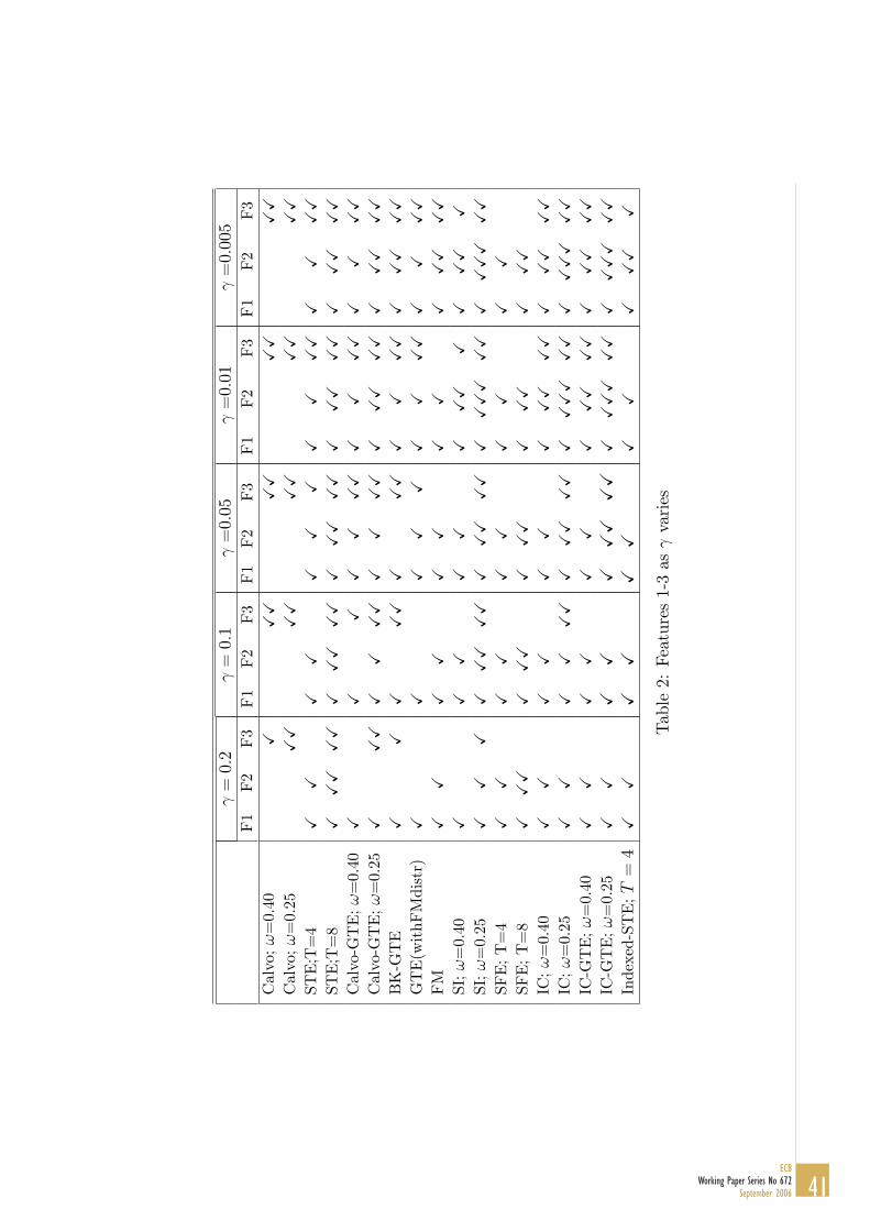
together and sytematically show how the change in in uences the modelsin terms of Features 1-3: In Table 2 we show how Features 1-3 fare foreach of the models at di�erent reference levels of : the benchmark level 0:2,0:1; 0:05; 0:01; and 0:005. Where there are weak and strong criteria (Features2 and 3) the more ticks indicates the stronger criteria being met.

Table2 Features 1-3 as varies.

Let us �rst take the benchmark case, which we have already explored.The only models to satisfy all three Features are the T = 8 simple Taylorcase and the SI with ! = 0:25, although the SI only meets the weak Feature2 (peaks at 4Q). Thus having long contracts is necessary but certainlynot su�cient to satisfy the stronger version of F2: the weaker 4Q version issatis�ed by several, but they all fail F3 except for SI with ! = 0:25. Turningto = 0:1, the value adopted by Mankiw and Reis (2002), we see that SImeets the strong criterion for Features 2 and 3. The Calvo-GTE and Calvowith Indexation (both with ! = 0:25) both satisfy the 4Q peak and thestrong version of Feature 3.Jumping to = 0:005, the FM value, something interesting happens. At

this low value of many models pass all three features: Strong Feature 2 and3 are satis�ed by: Simple Taylor 8, Calvo-GTE (! = 0:25), BK � GTE,SI(! = 0:25), FM, Calvo with Indexation (! = 0:4; ! = 0:25), Simple Taylor4 with indexation. Weak Feature 2 and strong 3 are also met by SimpleTaylor 4, Calvo-GTE (! = 0:4), FM �GTE: The important thing to noteis that at low values of , models without long average contract lengthsand backward looking indexation are showing peaks at 8Q or beyond. Themain conclusion to note is that this only happens in models where there is adistribution of contract lengths: for example the BK �GTE has an averageof 4:4 quarters, but peaks at 10 quarters. Indeed, this is best illustrated ifwe just look at the peak for di�erent values of in Table 3:

Table3: The peak response.

Note is that as varies some models do not change peak at all. Theseare the Calvo model: the peak is always at 1, and the simple models with justone contract length: simple Taylor and simple Fischer. In all other cases, as decreases, the peak gets pushed further back: and in all other cases thereis a distribution of contract lengths. In just three models is the distributiontruncated: in FM and FM-GTE there are no contracts longer than 4Q,

25ECB


and in Taylor-US GTE there are none greater than 8. In all others, theSI, Calvo-GTE, Indexed Calvo, BK-GTE, Calvo-GTE there are some verylong contracts which for practical computational purposes are truncated.This brings us to our conclusion about . When there is a distribution

of contracts, an decrease in will tend to delay the maximum impact if thereis already a hump shape. Note also that the assumption of indexation cana�ect the timing of the in ation peak in models with one type of contractlength if is su�ciently low but it has a larger e�ect on the in ation peakin models with a distribution.

7 Output and in ation

"We cannot be precise about the size or timing of all thesechannels. But the maximum e�ect on output is estimated to takeup to about one year. And the maximum impact of a change ininterest rates on consumer price in ation takes up to about twoyears" the Bank of England's webpage12.

Up until now we have been looking at in ation persistence on its own.However, it has long been argue that in ation peaks after output: the initialincrease in output generates the upward pressure on prices. For example,Christiano et al. (2005) �nd that in ation peaks at 8Q and output at 4Q. TheBank of England Quarterly Model has in ation peaking at 6Q and output at3Q. The above quote from the Bank of England on monetary policy re ectsthis conventional view.Clearly, the dynamic of output and in ation are governed at the aggregate

level by the quantity identity: (3): the sum of in ation and output growthmust add up to the rate of monetary growth in each period. The role of is very important: it determines the in ationary pressure on wages andprices resulting from an increase in output. A low value of means thatthis in ationary pressure works through more slowly so that the reaction ofin ation to output growth becomes slower. This also means that growth inoutput can be sustained for longer because the in ationary response is beingdelayed. The cumulative e�ect on in ation is �xed at 2%, since moneyis neutral in the long run. However, the cumulative a�ect on output will

12http://www.bankofengland.co.uk/monetarypolicy/how.htm


vary: the slower the response of in ation, the longer output can be abovethe long-run equilibrium.For both Calvo and simple Taylor, whilst the timing of the peak impact

on in ation does not depend on , the peak impact on output does. In thecase of Calvo, in ation always peaks on impact, and the output hump peakslater with lower . For all of the models with a distribution of contractlengths (except Calvo), a�ects both the timing of the output and in ationhumps, having a larger e�ect on the in ation peak.

Table4: output and in ation

In Table 4 we state the timing of the peak output growth and the dif-ference between the peak in ation and output. In the �rst table we can seethat in all models, the lower is ; the more delayed is the response of output.In the case of Calvo, in ation always peaks on impact, and the output humppeaks later with lower . This indicates that not only does the standardCalvo model generate the wrong in ation dynamics, but also reverses therelative timing of output and in ation peaks providing yet another reasonagainst the use of the Calvo model. In the simple Taylor and Fischer mod-els, in ation peaks at the length of the contract, output peaks earlier with asmaller gap when is lower.The most interesting thing to note about Table 4 is that for all of the

models except simple Taylor, Simple Fischer and Calvo, not only is the peakin ation after the output hump, but also the gap between the humps increasesas gets smaller. We can illustrate this with the BK-GTE:

F ig13: output and in ation in BK �GTEIn Fig 13a we depict the IR for output and in ation with the reference

value of = 0:2 there is a hump in in ation which peaks at 2Q and outputat 3Q. However, with the lower value of = 0:01, in ation peaks at 7Q andoutput at 4Q.

8 Conclusion

We have used the Generalized Taylor Economy, GTE, framework to evaluatethe performance of competing approaches for modelling nominal rigidities in

27ECB


the DGE models based on their potential in accounting for the observed in- ation dynamics. Recent empricial studies �nd that a monetary shock leadsto a hump shaped persistent in ation response. Due to the lack of consen-sus in the literature about the timing of the hump peak, we allow for threedi�erent values which corresponds to the moderate view (8Q), the Hawkishview (12Q) and the rapid view (4Q). We show how the assumptions regard-ing the distribution of contract lengths and the key parameters a�ect themodels' implications on in ation dynamics. Our �ndings can be summarisedas follows:

� In models with one type of contract length in ation always reachesits peak T � 1 quarters after the �rst period in which shock occurs.However, this type of model fails to generate enough persistence tosatisfy feature 3 with our reference value of = 0:2:When we allow for alow value of , which can be obtained, for example, by introducing �rmspeci�c capital, the problem goes away in the case of Taylor contracts.If you take the view that the hump peaks at 4 quarters, then the SimpleTaylor economy with average contract length of 4 can meet the threestylised facts. However, going beyond the 4 quarters would only bepossible if the model has long contracts. On the other hand, the simpleFischer model never generates enough persistence to satisfy Feature 3unless it has contract lengths in excess of 20 quarters.

� The presence of a distribution of contract lengths has signi�cant im-plications on the models' performance in accounting for the in ationdynamics. In particular, these models do not have problem in generat-ing persistent in ation response with plausible parameter values. Themain problem in this class of models is the timing of the hump. When = 0:2; most models cannot even make 4Q: The timing of the humpseems to be close with the most common contract durations. However,with a low value of ;these models can generate a hump at 8Q and evenbeyond. In this case, the predictions of such models are also consistentwith the common view that in ation peaks after output, and the gapbetween the two peaks is about 4 Quarters.

� The Calvo model does not capture in ation dynamics: in ation alwayspeaks on impact, and this precedes the peak in output. As getssmaller, it does not a�ect the timing of the peak in in ation, but itdoes a�ect the shape of the IR, and low values make the a�ect die o�


more slowly after the peak. This model should not be used to modelin ation dynamics.

� The assumption of indexation can a�ect the timing of the in ationhump, having a larger e�ect on the in ation peak in models with adistribution. In particular, IC and IC � GTE have very similar im-plications on in ation dynamics. However, the lack of direct evidencefor the indexation makes this class of models less plausible.

These �ndings lead us to conclude that models with a distribution, alongwith other frictions which helps to lower ; can be fairly successful in ex-plaining the in ation dynamics following a monetary shock. In fact, this�nding, to a large extent, explains the result obtained by Coenen and Levin(2004). Coenen and Levin (2004) show that a model with Taylor style con-tracts that allows for �rm speci�c capital and has a distribution of contractlengths �ts the German data very well without needing the assumption ofbackward-looking indexation. The same results also indicate that strongermicrofoundations are required in future work to include the distribution ofcontract lengths.

29ECB


References

Altig, D. E., Christiano, L. J., Eichenbaum, M. and Linde, J.: 2004, Firm-speci�c capital, nominal rigidities, and the business cycle, Working Pa-per 0416, Federal Reserve Bank of Cleveland .

Ascari, G.: 2000, Optimising agents, staggered wages and the persistence inthe real e�ects of money shocks, The Economic Journal 110, 664{686.

Batini, N.: 2002, Euro area in ation persistence, Working paper series201,European Central Bank .

Batini, N. and Nelson, E.: 2001, The lag from monetary policy actions toin ation: Friedman revisited, International Finance 4(3), 381{400.

Bils, M. and Klenow, P.: 2004, Some evidence on the importance of stickyprices, Journal of Political Economy 112(5), 947{985.

Calvo, G. A.: 1983, Staggered prices in a utility-maximizing framework,Journal of Monetary Economics 12(3), 383{398.

Chari, V. V., Kehoe, P. J. and McGrattan, E. R.: 2000, Sticky price modelsof the business cycle: Can the contract multiplier solve the persistenceproblem?, Econometrica 68(5), 1151{79.

Christiano, L. J., Eichenbaum, M. and Evans, C. L.: 2005, Nominal rigidi-ties and the dynamic e�ects of a shock to monetary policy, Journal ofPolitical Economy 113(1), 1{45.

Clark, T.: 2005, Disaggregate evidence on the persistence of consumer pricein ation, Journal of Applied Econometrics (forthcoming).

Coenen, G. and Levin, A. T.: 2004, Identifying the in uences of nominal andreal rigidities in aggregate price-setting behavior, Working paper series418, European Central Bank .

Cogley, T. and Sargent, T.: 2001, Evolving post-world war ii u.s. in ationdynamics, NBER Macroeconomics Annual pp. 331{372.

Dixon, H.: 2005, A uni�ed framework for understanding contract durationsin dynamic wage and price setting models, Mimeo .


Dixon, H. and Kara, E.: 2005a, How to compare Taylor and Calvo contracts:a comment on Michael Kiley, Journal of Money, Credit and Banking(forthcoming).

Dixon, H. and Kara, E.: 2005b, Persistence and nominal inertia in a general-ized taylor economy: how longer contracts dominate shorter contracts?,Working paper series 489, European Central Bank .

Dotsey, M., King, R. G. and Wolman, A. L.: 1999, State-dependent pric-ing and the general equilibrium dynamics of money and output, TheQuarterly Journal of Economics 114(2), 655{690.

Driscoll, J. C. and Holden, S.: 2003, In ation persistence and relative con-tracting, American Economic Review 93(4), 1369{1372.

Eichenbaum, M. and Fisher, J. D.: 2004, Evaluating the calvo model of stickyprices, NBER Working Paper No. 10617 .

Fischer, S.: 1977, Long-term contracts, rational expectations, and the opti-mal money supply rule, Journal of Political Economy 85(1), 191{205.

Fuhrer, J. and Moore, G.: 1995, In ation persistence, The Quarterly Journalof Economics 110(1), 127{59.

Gali, J. and Gertler, M.: 1999, In ation dynamics: A structural econometricanalysis, Journal of Monetary Economics 44(2), 195{222.

Huang, K. X. D., Liu, Z. and Phaneuf, L.: 2004, Why does the cyclicalbehavior of real wages change over time?, American Economic Review94(4), 836{856.

Kiley, M.: 2005, A quantitative comparison of sticky-price and sticky-information models of price setting, Mimeo .

Levin, A. T. and Piger, J. M.: 2004, Is in ation persistence intrinsic in in-dustrial economies?, Working paper series 334, European Central Bank.

Mankiw, N. G. and Reis, R.: 2002, Sticky information versus sticky prices:A proposal to replace the new keynesian phillips curve, The QuarterlyJournal of Economics 117(4), 1295{1328.

31ECB


Nelson, E.: 1998, Sluggish in ation and optimizing models of the businesscycle, Journal of Monetary Economics 42(2), 303{322.

Pivetta, F. and Reis, R.: 2004, The persistence of in ation in the unitedstates, Mimeo .

Roberts, J.: 2005, How well does the new keynesian sticky price model �tthe data, Contributions to Macroeconomics 5(1).

Smets, F. and Wouters, R.: 2003, An estimated dynamic stochastic generalequilibrium model of the euro area, Journal of the European EconomicAssociation 1(5), 1123{1175.

Smets, F., Wouters, R. and de Walque, G.: 2005, Price setting in generalequilibrium: Alternative speci�cations, Mimeo .

Taylor, J. B.: 1980, Staggered wage and price setting in macroeconomics,Journal of Political Economy 88(1), 1{23.

Taylor, J. B.: 2000, Low in ation, pass-through, and the pricing power of�rms, European Economic Review 44(7), 1389{1408.

Woodford, M.: 2003, Interest and prices: Foundations of a theory of mone-tary policy, Princeton Univeristy Press, Princeton, NJ .


Appendix.

A Model

In this section, we describe the GTE framework in detail and then discuss themodi�cations required to the model when we consider di�erent assumptionregarding the wage-setting.

A.1 Generalised Taylor Economy (GTE)

A.1.1 Firms

There is a continuum of �rms f 2 [0; 1]; each producing a single di�erentiatedgood Y (f), which are combined to produce a �nal consumption good Y: Theproduction function here is CES with constant returns and correspondingunit cost function P

Yt =

�Z 1

0

Yt(f)��1� df

� ��1

(9)

Pt =

�Z 1

0

P 1��ft df

� 11��

(10)

The demand for the output of �rm f is

Yft =

�PftPt

��Yt (11)

Each �rm f sets the price Pft and takes the �rm-speci�c wage rate Wft asgiven. Labor Lft is the only input so that the inverse production function is

Lft =

�Yft�

� 1�

(12)

Where � � 1 represents the degree of diminishing returns, with � = 1 beingconstant returns. The �rm chooses fPft;Yft; Lftg to maximize pro�ts subjectto (11,12), yields the following solutions for price, output and employment

33ECB


at the �rm level given fYt;Wft; Ptg

Pft =

��

� � 1

��1=�

�WftY

1��

ft (13)

Yft = �1

�Wft

Pt

��"Y

"��

t (14)

Lft = �2

�Wft

Pt

��"Y

"�t (15)

where " = ��(1��)+� > 1 �1 =

��1��"

��"��" �2 =�

��1��"

�"�"(��1�) :

Price is a markup over marginal cost, which depends on the wage rateand the output level (when � < 1): output and employment depend on thereal wage and total output in the economy.

A.1.2 Uniform GTE: the structure of contracts.

The economy is divided into many sectors where the i�th sector has a simpleTaylor contract length of T = i periods. The share of each sector is givenby �i with

PNi=1 �i = 1: Since we consider only uniform GTE s, in each sector

i; there are i the cohorts which are of equal size. As a result, �ii�1 contracts

are reset in each period in sector i.

A.1.3 Household-Unions and Wage Setting

Households h 2 [0; 1] have preferences de�ned over consumption, labour, andreal money balances. The expected life-time utility function takes the form

Uh = Et

24 1Xt=0

�tu(Cht;Mht

Pt; 1�Hht| {z }

Lht

)

35 (16)

where Cht,�Mht

Pt

�; Hht; Lht are household h

0s consumption, end-of period

real money balances, hours worked, and leisure respectively, t is an index fortime, 0 < � < 1 is the discount factor, and each household has the same owutility function u, which is assumed to take the form

U(Cht) + � ln(Mht

Pt) + V (1�Hht) (17)


Each household-union belongs to a particular sector and wage-settingcohort within that sector (recall, that each household is twinned with �rmf = h). Since the household acts as a monopoly union, hours worked aredemand determined, being given by the (15).The household's budget constraint is given by

PtCht+Mht+Xst+1

Q(st+1 j st)Bh(st+1) �Mht�1+Bht+WhtHht+�ht+Tht (18)

where Bh(st+1) is a one-period nominal bond that costs Q(st+1 j st) at

state st and pays o� one dollar in the next period if st+1 is realized. Bhtrepresents the value of the household's existing claims given the realized stateof nature. Mht denotes money holdings at the end of period t. Wht is thenominal wage, �ht is the pro�ts distributed by �rms andWhtHht is the labourincome. Finally, Tt is a nominal lump-sum transfer from the government.The households optimization breaks down into two parts. First, there is

the choice of consumption, money balances and one-period nominal bonds tobe transferred to the next period to maximize expected lifetime utility (16)given the budget constraint (18). The �rst order conditions derived from theconsumer's problem are as follows:

uct = �RtEt

�PtPt+1

uct+1

�(19)

Xst+1

Q(st+1 j st) = �Etuct+1PtuctPt+1

=1

Rt(20)

�PtMt

= uct � �EtPtPt+1

uct+1 (21)

Equation (19) is the Euler equation, (20) gives the gross nominal inter-est rate and (21) gives the optimal allocation between consumption and realbalances. Note that the index h is dropped in equations (19) and (21), whichre ects our assumption of complete contingent claims markets for consump-tion and implies that consumption is identical across all households in eachperiod (Cht = Ct)

13:Household h in sector i chooses wage to maximize lifetime utility given

labour demand (15) and the additional constraint that nominal wage will

13See Ascari (2000).

35ECB


be �xed for Ti periods in which the aggregate output and price level aregivenfYt; Ptg. Since the reset wage at time t will only hold for Ti periods,we have the following �rst-order condition:

Xit =

�"

"� 1

�266664Et

Ti�1Xs=0

�s [VL (1�Ht+s) (Kt+s)]

Et

Ti�1Xs=0

�shuc(Ct+s)Pt+s

Kt+s

i377775 (22)

where Kt = �2P"t Y

"�t collects all of the terms in (15) which the union

treats as exogenous.Equation (22) shows that the optimal wage is a constant "mark-up" (given

by ""�1) over the ratio of marginal utilities of leisure and marginal utility from

consumption within the contract duration, from t to t+Ti�1: When Ti = 2,this equation reduces to the �rst order condition in Ascari (2000).

A.2 Generalised Fischer Economy (GFE)

In a model with Fischer (1977) contracts, household h in sector i chooseschooses a trajectory of wages, one for each period for the whole length of thecontract. The �rst order condition now becomes:

Xit+s =

�"

"� 1

�24Et [VL (1�Ht+s)]Et

huc(Ct+s)Pt+s

i35 (23)

where s = 0:::Ti � 1: Note that the equation is identical to the the wagelevel in which wages are fully exible.

A.3 Calvo with Indexation: Woodford (2003)

As in the simple Calvo (1983) pricing model, there is the reset probabilityor hazard rate !, which gives the non-duration dependent probability thata �rm/union will have the option to reset its wage in any period and house-hold h chooses wage to maximize lifetime utility given labour demand (15)during the lifetime of the contract. But now maximization problem also in-cludes lagged in ation due to the assumption of indexation. The �rst ordercondition is given by:


Xt =

�"

"� 1

�24 EtP1

s=0((1� !) �)s [VL (1�Ht+s) (Kt+s)]

EtP1

s=0((1� !) �)shuc(Ct+s)Pt+s

�Pt�1+iPt�1

�aKt+s

i35 (24)

where 0 � a � 1 measures the degree of indexation to the past in ationrate. a = 0 gives the wage setting rule for the simple Calvo Economy. Notethat the index i is dropped in this equation due reason that in the Calvopricing model there is only one reset wage (see Dixon and Kara (2005b) fora discussion).

A.4 The GTE with Indexation

When we allow for indexation in the GTE; the optimal wage rule changesfrom (22) to:

Xit =

�"

"� 1

�266664Et

Ti�1Xs=0

�s [VL (1�Ht+s) (Kt+s)]

Et

Ti�1Xs=0

�shuc(Ct+s)Pt+s

�Pt�1+iPt�1

�aKt+s

i377775 (25)

B Linearized Model

This section presents equation which are the linearized counterparts to theequations outlined in the pervious section of the appendix. We start withthe wage-setting rules for di�erent contracts. Lower-case letters denotes log-deviations of variables from the steady state

B.1 Generalised Taylor Economy (GTE)

The linearized version of the equations described in the previous section arefollows. As in Dixon and Kara (2005b), the wage setting rule is summarisedfor the reset wage which is set by the cohort changing contracts at t andremains in force for i periods.

37ECB


xit =1

Ti�1Xs=0

�s

"Ti�1Xs=0

�s [pt+s + yt+s]

#(26)

where

=�LL+ �cc(� + �(1� �))

� + �(1� �) + ��LL

(27)

The rest of the equations are given by

wit =

Ti�1Xj=0

1

Tixit�j (28)

pit = wit +

�1� ��

�yit (29)

yit = �(pt � pit) + yt (30)

pt =NXi=1

�ipit (31)

yt = mt � pt (32)

In addition, the money supply follows a AR(1) process;

mt = mt�1 + ln(�t); ln(�t) = v�t�1 + �t (33)

where 0 < v < 1 and �t is a white noise process with zero mean and a�nite variance.

B.2 Generalised Fischer Economy (GFE)

Log-Linearising version of (23) is given by

xit+s = pt+s + yt+s (34)

Sectoral wage index can be expressed as


wit =

TiXs=0

1

TiEt�sxit (35)

Replacing (26) and (28) with (34) and (35) from the above equations,respectively, gives the equilibrium conditions in the GFE:

B.3 Calvo with Indexation: Woodford (2003)

Log-Linearising (24) and putting for simplicity � = a = 1 yields

xt = ! (pt + yt)� (1� !)�t + (1� !)xt+1 (36)

The evolution of the aggregate wage index is given by

wt = !xt + (1� !) (wt�1 + �t�1) (37)

Finally, the aggregate price index is

pt = wt +

�1� ��

�yt (38)

By inserting (38) and (37) into (36), after some algebra, we obtain thehybrid phillips curve reported in the main text.

B.4 GTE with Indexation

When we allow partial indexation in the GTE; the wage setting rule changesto

xt =1

Ti�1Xs=0

�s

"Ti�1Xs=0

�sipt+s +

Ti�1Xs=0

�syt+s �Ti�2Xs=0

Ti�1Xk=s+1

�k�t+s

#(39)

Sectoral wage index changes from (28) to

wit =

Ti�1Xj=0

1

Ti(xit�j � �t�1�j)

39ECB


B.5 Fuhrer and Moore (1995) and FM �GTEFuhrer and Moore's model does not have microfoundations. We modi�edthe equations to allow for an economy with many sectors, each with a Fuhrerand Moore contract of a particular length. In this case, unions care aboutrelative real wages within the contract duration.

xit � pt =Ti�1Ps=0

fsvt+s + Ti�1Pi=0

fsyt+s (40)

where fs =1Ti:

The aggregate index of real wages is given by

vt =NXi=1

�ivit (41)

where

vit =

Ti�1Xj=0

1

Ti(xit�s � pt�s)

Equations (40) and (41) along with the equations (28)-(32) characterizethe equilibrium in the FM-GTE. When Ti = 4 and fs = 0:25 + (1:5 � s)q;q 2 (0; 1

6) , (41) reduces to the wage setting rule as in Fuhrer and Moore

(1995).


=0:2

F1

F2

F3

Calvo;!=0.40

XCalvo;!=0.25

XX

STE;T=4

XX

STE;T=8

XXX

XX

Calvo-GTE;!=0.40

XCalvo-GTE;!=0.25

XXX

BK-GTE

XX

GTE(withFMdistr)

XFM

XX

SI;!=0.40

XSI;!=0.25

XX

XSFE;T=4

XX

SFE;T=8

XXX

IC;!=0.40

XX

IC;!=0.25

XX

IC-GTE;!=0.40

XX

IC-GTE;!=0.25

XX

Indexed-STE;T=4

XX

=0:1

F1

F2

F3

XX

XX

XX

XXX

XX

XX

XX

XX

XXX

X XX

XX

XXX

XX

XX

XXX

XX

XX

XX

XX

XX

XX

=0:05

F1

F2

F3 XX

XX

XX

XX

XX

XX

XX

XX

XX

XX

XXX

XX

XX

XX

XX

XX

XX

XX

XXX

XX

XXX

XX

XX

XXX

XX

XX

=0:01

F1

F2

F3

XX

XX

XX

XX

XXX

XX

XX

XX

XXX

XX

XX

XX

XX

XX

XX

XXX

XX

XXX

XX

XX

XXX

XXX

XX

XXXX

XX

XXX

XX

XXXX

XX

XX

=0:005

F1

F2

F3

XX

XX

XX

XX

XXX

XX

XX

XX

XXX

XX

XXX

XX

XX

XX

XXX

XX

XXX

XX

XXX

XX

XX

XXX

XXX

XX

XXXX

XX

XXX

XX

XXXX

XX

XXX

X

Table2:Features1-3as varies

41ECB


0.2 0.1 0.05 0.01 0.005

Calvo; !=0.40 1 1 1 1 1

Calvo; !=0.25 1 1 1 1 1

STE; T=4 4 4 4 4 4

STE; T=8 8 8 8 8 8

Calvo-GTE; !=0.40 2 3 4 5 6

Calvo-GTE; !=0.25 3 4 5 9 11

BK-GTE 2 2 2 7 10

GTE(with FM distr) 3 3 4 4 4

FM 4 4 4 7 8

SI; ! = 0:40 3 5 6 9 11

SI; ! = 0:25 5 8 11 16 19

SFE; T=4 4 4 4 4 4

SFE; T=8 8 8 8 8 8

IC; ! = 0:40 4 5 6 9 11

IC; ! = 0:25 5 6 8 13 16

IC-GTE; ! = 0:40 4 4 6 9 11

IC-GTE; ! = 0:25 5 6 8 13 16

Indexed-STE; T = 4 4 4 5 7 9

Table 3: The peak response of in ation (in quarters)

0.2 0.1 0.05 0.01 0.005

Calvo; !=0.40 -1 -2 -2 -3 -4Calvo; !=0.25 -2 -2 -3 -4 -4STE; T=4 2 2 1 1 0STE; T=8 5 5 4 3 3Calvo-GTE; !=0.40 0 0 1 1 2Calvo-GTE; !=0.25 0 1 1 4 6BK-GTE -1 -1 -1 3 5GTE(with FM distr) 1 1 2 1 1FM 2 2 2 4 5SI; != 0:40 1 2 3 5 6SI; != 0:25 2 4 7 10 13SFE; T=4 2 2 1 1 1SFE; T=8 4 4 3 2 2IC; != 0:40 2 3 3 5 7IC; != 0:25 2 3 5 9 11IC-GTE; != 0:40 2 2 3 5 6IC-GTE; != 0:25 3 5 8 11Indexed-STE; T = 4 2 2 2 4 5

Table 4: The di�etrence between the peaks


Figure 1: Response of In ation in the Calvo Economy

Figure 2: Response of In ation in the Simple Taylor Economy

43ECB


Figure 3: Response of In ation in the Calvo-GTE and the Calvo Economy

Figure 4: BK �GTE :Distribution


Figure 5: Response of In ation in the BK-GTE

Figure 6: Response of In ation in the Simple Fischer Economy

45ECB


Figure 7: Response of In ation in the Simple Fischer Economy and SI

Figure 8: Response of In ation in the FM and FM-GTE


Figure 9: Response of In ation in the Indexed-Calvo

Figure 10: Response of In ation in the Indexed-Taylor

47ECB


Figure 11: Response of In ation in the IC-GTE and IC


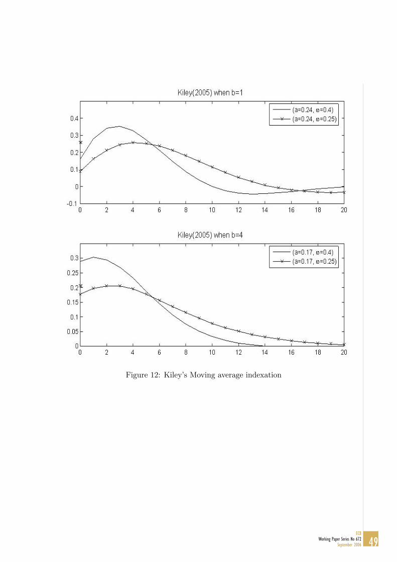
Figure 12: Kiley's Moving average indexation

49ECB


Figure 13: Output and In ation Responses in BK �GTE


51ECB


European Central Bank Working Paper Series

For a complete list of Working Papers published by the ECB, please visit the ECB’s website(http://www.ecb.int)

635 “Identifying the role of labor markets for monetary policy in an estimated DSGE model”by K. Christoffel, K. Kuester and T. Linzert, June 2006.

636 “Exchange rate stabilization in developed and underdeveloped capital markets”by V. Chmelarova and G. Schnabl, June 2006.

637 “Transparency, expectations, and forecasts” by A. Bauer, R. Eisenbeis, D. Waggoner andT. Zha, June 2006.

638 “Detecting and predicting forecast breakdowns” by R. Giacomini and B. Rossi, June 2006.

639 “Optimal monetary policy with uncertainty about financial frictions” by R. Moessner, June 2006.

640 “Employment stickiness in small manufacturing firms” by P. Vermeulen, June 2006.

641 “A factor risk model with reference returns for the US dollar and Japanese yen bond markets”by C. Bernadell, J. Coche and K. Nyholm, June 2006.

642 “Financing constraints and firms’ cash policy in the euro area” by R. Pál and A. Ferrando, June 2006.

643 “Inflation forecast-based-rules and indeterminacy: a puzzle and a resolution” by P. Levine,P. McAdam and J. Pearlman, June 2006.

644 “Adaptive learning, persistence, and optimal monetary policy” by V. Gaspar, F. Smets andD. Vestin, June 2006.

645 “Are internet prices sticky?” by P. Lünnemann and L. Wintr, June 2006.

646 “The Dutch block of the ESCB multi-country model” by E. Angelini, F. Boissay andM. Ciccarelli, June 2006.

647 “The economic effects of exogenous fiscal shocks in Spain: a SVAR approach”by F. de Castro Fernández and P. Hernández de Cos, June 2006.

648 “Firm-specific production factors in a DSGE model with Taylor price setting” by G. de Walque,F. Smets and R. Wouters, June 2006.

649 “Monetary and fiscal policy interactions in a New Keynesian model with capital accumulation andnon-Ricardian consumers” by C. Leith and L. von Thadden, June 2006.

650 “A structural break in the effects of Japanese foreign exchange intervention on yen/dollarexchange rate volatility” by E. Hillebrand and G. Schnabl, June 2006.

651 “On the determinants of external imbalances and net international portfolio flows: a globalperspective” by R. A. De Santis and M. Lührmann, July 2006.


652 “Consumer price adjustment under the microscope: Germany in a period of low inflation”by J. Hoffmann and J.-R. Kurz-Kim, July 2006.

653 “Acquisition versus greenfield: the impact of the mode of foreign bank entry on information andbank lending rates” by S. Claeys and C. Hainz, July 2006.

654 “The German block of the ESCB multi-country model” by I. Vetlov and T. Warmedinger, July 2006.

655

656 “Public debt and long-term interest rates: the case of Germany, Italy and the USA” by P. Paesani,R. Strauch and M. Kremer, July 2006.

657 “The impact of ECB monetary policy decisions and communication on the yield curve”by C. Brand, D. Buncic and J. Turunen, July 2006.

658 “The response of firms‘ investment and financing to adverse cash flow shocks: the role of bankrelationships” by C. Fuss and P. Vermeulen, July 2006.

659 “Monetary policy rules in the pre-EMU era: Is there a common rule?” by M. Eleftheriou,D. Gerdesmeier and B. Roffia, July 2006.

660 “The Italian block of the ESCB multi-country model” by E. Angelini, A. D’Agostino andP. McAdam, July 2006.

661 “Fiscal policy in a monetary economy with capital and finite lifetime” by B. Annicchiarico,N. Giammarioli and A. Piergallini, July 2006.

662 “Cross-border bank contagion in Europe” by R. Gropp, M. Lo Duca and J. Vesala, July 2006.

663 “Monetary conservatism and fiscal policy” by K. Adam and R. M. Billi, July 2006.

664 “Fiscal convergence before entering the EMU” by L. Onorante, July 2006.

665 “The euro as invoicing currency in international trade” by A. Kamps, August 2006.

666 “Quantifying the impact of structural reforms” by E. Ernst, G. Gong, W. Semmler andL. Bukeviciute, August 2006.

667 “The behaviour of the real exchange rate: evidence from regression quantiles” by K. Nikolaou,August 2006.

668 “Declining valuations and equilibrium bidding in central bank refinancing operations”by C. Ewerhart, N. Cassola and N. Valla, August 2006.

669 “Regular adjustment: theory and evidence” by J. D. Konieczny and F. Rumler, August 2006.

670 “The importance of being mature: the effect of demographic maturation on globalper-capita GDP” by R. Gómez and P. Hernández de Cos, August 2006.

671 “Business cycle synchronisation in East Asia” by F. Moneta and R. Rüffer, August 2006.

“Fiscal and monetary policy in the enlarged European Union” by S. Pogorelec, July 2006.

53ECB


672 “Understanding inflation persistence: a comparison of different models” by H. Dixonand E. Kara, September 2006.

ISSN 1561081-0

9 7 7 1 5 6 1 0 8 1 0 0 5

Documents

Understanding inflation persistence: a comparison of different models