Embed Size (px)
Citation preview

Pearson New International Edition
International_PCL_TP.indd 1 7/29/13 11:23 AM
Introduction to Robotics:Mechanics and Control
John J. CraigThird Edition

Pearson Education Limited
Edinburgh Gate
Harlow
Essex CM20 2JE
England and Associated Companies throughout the world
Visit us on the World Wide Web at: www.pearsoned.co.uk
© Pearson Education Limited 2014
All rights reserved. No part of this publication may be reproduced, stored in a retrieval system, or transmitted
in any form or by any means, electronic, mechanical, photocopying, recording or otherwise, without either the
prior written permission of the publisher or a licence permitting restricted copying in the United Kingdom
issued by the Copyright Licensing Agency Ltd, Saffron House, 6–10 Kirby Street, London EC1N 8TS.
All trademarks used herein are the property of their respective owners. The use of any trademark
in this text does not vest in the author or publisher any trademark ownership rights in such
trademarks, nor does the use of such trademarks imply any affi liation with or endorsement of this
book by such owners.
ISBN 10: 1-269-37450-8ISBN 13: 978-1-269-37450-7
British Library Cataloguing-in-Publication Data
A catalogue record for this book is available from the British Library
Printed in the United States of America
Copyright_Pg_7_24.indd 1 7/29/13 11:28 AM
ISBN 10: 1-292-04004-1ISBN 13: 978-1-292-04004-2
ISBN 10: 1-292-04004-1ISBN 13: 978-1-292-04004-2

Table of Contents
P E A R S O N C U S T O M L I B R A R Y
I
Chapter∞ѳѢ∞IntroductionѢ
1
1John J. Craig
Chapter∞ѴѢ∞Spatial∞TransformationsѢ
19
19John J. Craig
Chapter∞ѵѢ∞Forward∞KinematicsѢ
62
62John J. Craig
Chapter∞ҐѢ∞Inverse∞KinematicsѢ
101
101John J. Craig
Chapter∞ґѢ∞Velocitiesў∞Static∞Forcesў∞and∞JacobiansѢ
135
135John J. Craig
Chapter∞әѢ∞DynamicsѢ
165
165John J. Craig
Chapter∞‐Ѣ∞Trajectory∞PlanningѢ
201
201John J. Craig
Chapter∞ℓѢ∞Mechanical∞Design∞of∞RobotsѢ
230
230John J. Craig
Chapter∞№Ѣ∞Linear∞ControlѢ
262
262John J. Craig
Chapter∞ѳѲѢ∞NonџLinear∞ControlѢ
290
290John J. Craig
Chapter∞ѳѳѢ∞Force∞ControlѢ
317
317John J. Craig
Chapter∞ѳѴѢ∞Programming∞Languages∞and∞SystemsѢ
339
339John J. Craig
Appendix∞AѢ∞Trigonometric∞Identities
354
354John J. Craig

II
Appendix∞BѢ∞The∞ѴҐ∞AngleџSet∞Conventions
356
356John J. Craig
Appendix∞CѢ∞Some∞InverseџKinematic∞Formulas
359
359John J. Craig
Solutions∞to∞Selected∞Exercises
361
361John J. Craig
369
369Index

C H A P T E R 1
Introduction
1.1 BACKGROUND
1.2 THE MECHANICS AND CONTROL OF MECHANICAL MANIPULATORS
1.3 NOTATION
1.1 BACKGROUND
The history of industrial automation is characterized by periods of rapid change inpopular methods. Either as a cause or, perhaps, an effect, such periods of change inautomation techniques seem closely tied to world economics. Use of the industrialrobot, which became identifiable as a unique device in the 1960s [1], along withcomputer-aided design (CAD) systems and computer-aided manufacturing (CAM)systems, characterizes the latest trends in the automation of the manufacturingprocess. These technologies are leading industrial automation through anothertransition, the scope of which is still unknown [2].
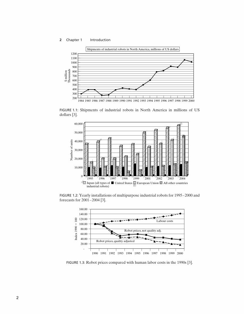
In North America, there was much adoption of robotic equipment in the early1980s, followed by a brief pull-back in the late 1980s. Since that time, the market hasbeen growing (Fig. 1.1), although it is subject to economic swings, as are all markets.
Figure 1.2 shows the number of robots being installed per year in the majorindustrial regions of the world. Note that Japan reports numbers somewhat dif-ferently from the way that other regions do: they count some machines as robotsthat in other parts of the world are not considered robots (rather, they would besimply considered ‘‘factory machines’’). Hence, the numbers reported for Japan aresomewhat inflated.
A major reason for the growth in the use of industrial robots is their decliningcost. Figure 1.3 indicates that, through the decade of the 1990s, robot prices droppedwhile human labor costs increased. Also, robots are not just getting cheaper, theyare becoming more effective—faster, more accurate, more flexible. If we factorthese quality adjustments into the numbers, the cost of using robots is dropping evenfaster than their price tag is. As robots become more cost effective at their jobs,and as human labor continues to become more expensive, more and more industrialjobs become candidates for robotic automation. This is the single most importanttrend propelling growth of the industrial robot market. A secondary trend is that,economics aside, as robots become more capable they become able to do more andmore tasks that might be dangerous or impossible for human workers to perform.
The applications that industrial robots perform are gradually getting moresophisticated, but it is still the case that, in the year 2000, approximately 78%of the robots installed in the US were welding or material-handling robots [3].
From Chapter 1 of Introduction to Robotics: Mechanics and Control, Third Edition. John J. Craig.
Copyright © 2005 by Pearson Education, Inc. All rights reserved.
1
2 Chapter 1 Introduction
1984 1985 1986 1987 1988 1989 1990 1991 1992 1993 1994 1995 1996 1997 1998 1999 2000200
300
400
500
600
700
800
900
1000
1100
1200
$ m
illi
on
Th
ou
san
ds
Shipments of industrial robots in North America, millions of US dollars
FIGURE 1.1: Shipments of industrial robots in North America in millions of USdollars [3].
1995 1996 1997 1998 1999 2001 2002 2003 20040
10,000
20,000
30,000
40,000
50,000
60,000
Nu
mb
er o
f u
nit
s
Japan (all types ofindustrial robots)
United States European Union All other countries
FIGURE 1.2: Yearly installations of multipurpose industrial robots for 1995–2000 andforecasts for 2001–2004 [3].
-
20.00
1990 1991 1992 1993 1994 1995 1996 1997 1998 1999 2000
40.00
60.00
80.00
100.00
120.00
140.00
160.00
Ind
ex 1
990
� 1
00 Labour costs
Robot prices, quality adjusted
Robot prices, not quality adj.
FIGURE 1.3: Robot prices compared with human labor costs in the 1990s [3].
2
Section 1.1 Background 3
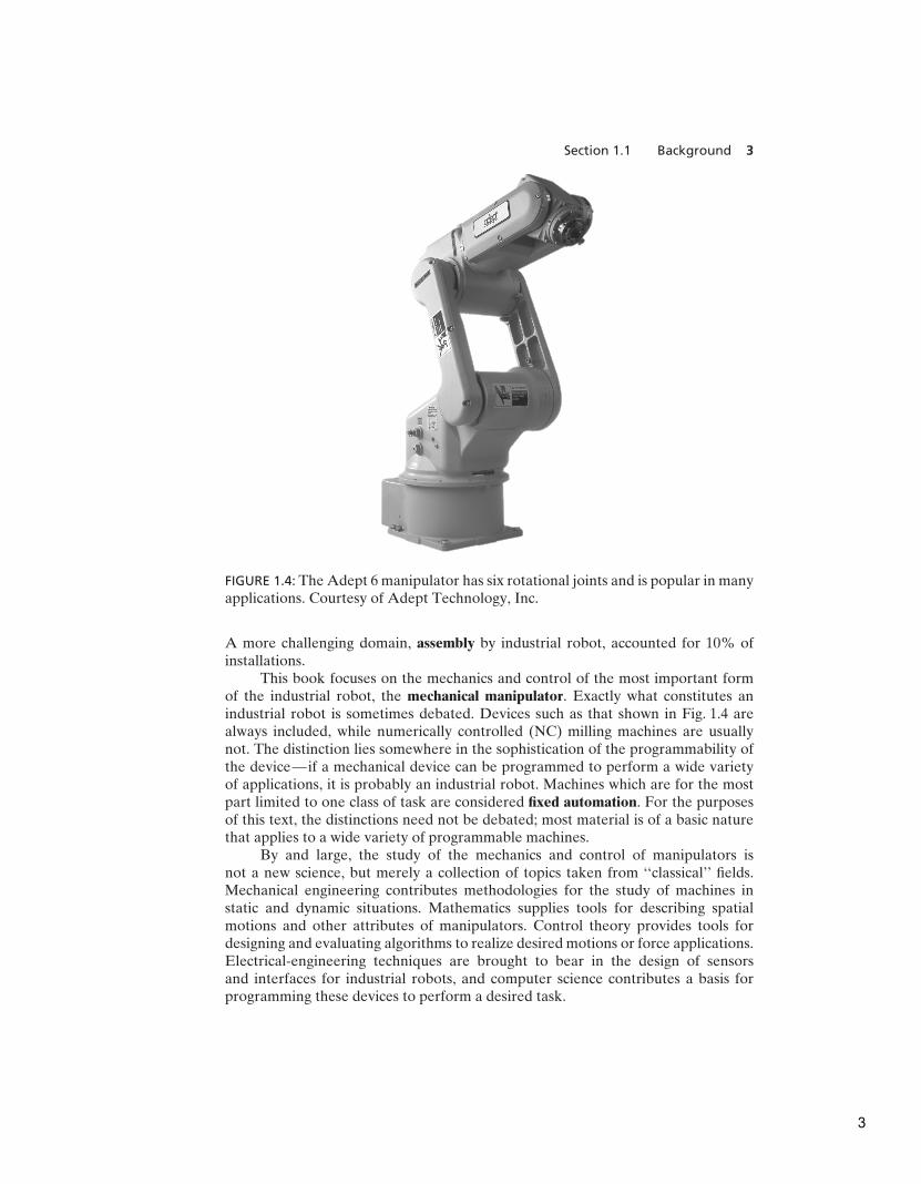
FIGURE 1.4: The Adept 6 manipulator has six rotational joints and is popular in manyapplications. Courtesy of Adept Technology, Inc.
A more challenging domain, assembly by industrial robot, accounted for 10% ofinstallations.
This book focuses on the mechanics and control of the most important formof the industrial robot, the mechanical manipulator. Exactly what constitutes anindustrial robot is sometimes debated. Devices such as that shown in Fig. 1.4 arealways included, while numerically controlled (NC) milling machines are usuallynot. The distinction lies somewhere in the sophistication of the programmability ofthe device—if a mechanical device can be programmed to perform a wide varietyof applications, it is probably an industrial robot. Machines which are for the mostpart limited to one class of task are considered fixed automation. For the purposesof this text, the distinctions need not be debated; most material is of a basic naturethat applies to a wide variety of programmable machines.
By and large, the study of the mechanics and control of manipulators isnot a new science, but merely a collection of topics taken from ‘‘classical’’ fields.Mechanical engineering contributes methodologies for the study of machines instatic and dynamic situations. Mathematics supplies tools for describing spatialmotions and other attributes of manipulators. Control theory provides tools fordesigning and evaluating algorithms to realize desired motions or force applications.Electrical-engineering techniques are brought to bear in the design of sensorsand interfaces for industrial robots, and computer science contributes a basis forprogramming these devices to perform a desired task.
3

4 Chapter 1 Introduction
1.2 THE MECHANICS AND CONTROL OF MECHANICAL MANIPULATORS
The following sections introduce some terminology and briefly preview each of thetopics that will be covered in the text.
Description of position and orientation
In the study of robotics, we are constantly concerned with the location of objects inthree-dimensional space. These objects are the links of the manipulator, the partsand tools with which it deals, and other objects in the manipulator’s environment.At a crude but important level, these objects are described by just two attributes:position and orientation. Naturally, one topic of immediate interest is the mannerin which we represent these quantities and manipulate them mathematically.
In order to describe the position and orientation of a body in space, we willalways attach a coordinate system, or frame, rigidly to the object. We then proceedto describe the position and orientation of this frame with respect to some referencecoordinate system. (See Fig. 1.5.)
Any frame can serve as a reference system within which to express theposition and orientation of a body, so we often think of transforming or changing
the description of these attributes of a body from one frame to another. Chapter 2discusses conventions and methodologies for dealing with the description of positionand orientation and the mathematics of manipulating these quantities with respectto various coordinate systems.
Developing good skills concerning the description of position and rotation ofrigid bodies is highly useful even in fields outside of robotics.
Forward kinematics of manipulators
Kinematics is the science of motion that treats motion without regard to the forceswhich cause it. Within the science of kinematics, one studies position, velocity,
Z
Z
X
X
X
Z
Z
X
YY
Y
Y
FIGURE 1.5: Coordinate systems or ‘‘frames’’ are attached to the manipulator and toobjects in the environment.
4
Section 1.2 The mechanics and control of mechanical manipulators 5
acceleration, and all higher order derivatives of the position variables (with respectto time or any other variable(s)). Hence, the study of the kinematics of manipulatorsrefers to all the geometrical and time-based properties of the motion.
Manipulators consist of nearly rigid links, which are connected by joints thatallow relative motion of neighboring links. These joints are usually instrumentedwith position sensors, which allow the relative position of neighboring links to bemeasured. In the case of rotary or revolute joints, these displacements are calledjoint angles. Some manipulators contain sliding (or prismatic) joints, in which therelative displacement between links is a translation, sometimes called the jointoffset.
The number of degrees of freedom that a manipulator possesses is the numberof independent position variables that would have to be specified in order to locateall parts of the mechanism. This is a general term used for any mechanism. Forexample, a four-bar linkage has only one degree of freedom (even though thereare three moving members). In the case of typical industrial robots, because amanipulator is usually an open kinematic chain, and because each joint position isusually defined with a single variable, the number of joints equals the number ofdegrees of freedom.
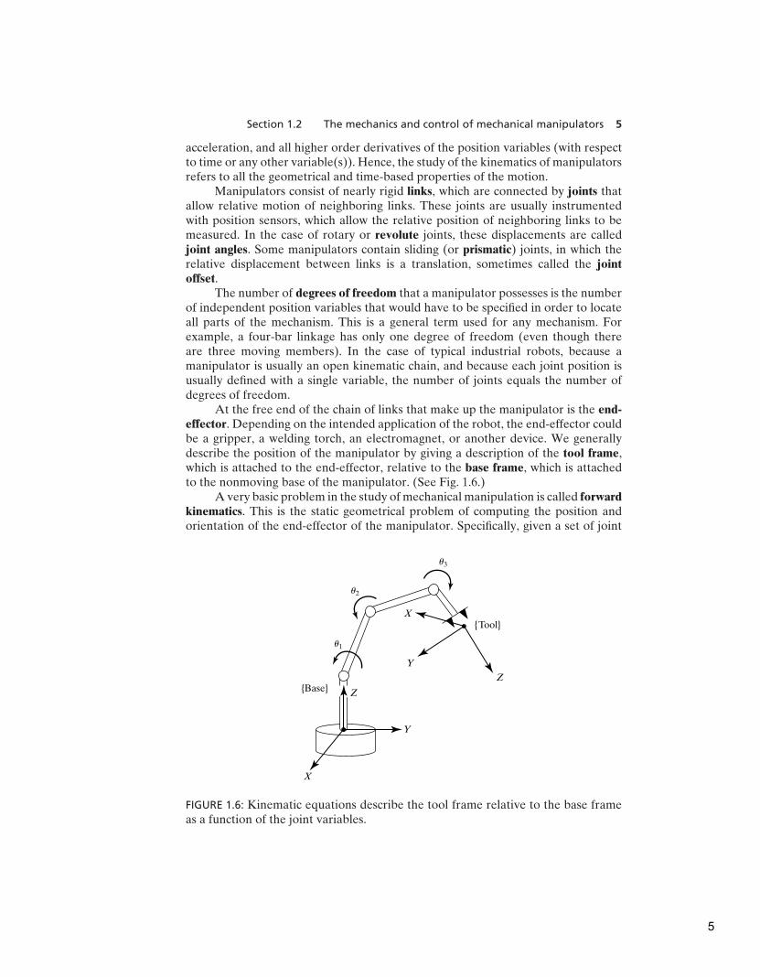
At the free end of the chain of links that make up the manipulator is the end-effector. Depending on the intended application of the robot, the end-effector couldbe a gripper, a welding torch, an electromagnet, or another device. We generallydescribe the position of the manipulator by giving a description of the tool frame,which is attached to the end-effector, relative to the base frame, which is attachedto the nonmoving base of the manipulator. (See Fig. 1.6.)
A very basic problem in the study of mechanical manipulation is called forwardkinematics. This is the static geometrical problem of computing the position andorientation of the end-effector of the manipulator. Specifically, given a set of joint
X
X
Z
Z
Y
Y
{Tool}
{Base}
u2
u1
u3
FIGURE 1.6: Kinematic equations describe the tool frame relative to the base frameas a function of the joint variables.
5

6 Chapter 1 Introduction
angles, the forward kinematic problem is to compute the position and orientation ofthe tool frame relative to the base frame. Sometimes, we think of this as changingthe representation of manipulator position from a joint space description into aCartesian space description.1 This problem will be explored in Chapter 3.
Inverse kinematics of manipulators
In Chapter 4, we will consider the problem of inverse kinematics. This problemis posed as follows: Given the position and orientation of the end-effector of themanipulator, calculate all possible sets of joint angles that could be used to attainthis given position and orientation. (See Fig. 1.7.) This is a fundamental problem inthe practical use of manipulators.
This is a rather complicated geometrical problem that is routinely solvedthousands of times daily in human and other biological systems. In the case of anartificial system like a robot, we will need to create an algorithm in the controlcomputer that can make this calculation. In some ways, solution of this problem isthe most important element in a manipulator system.
We can think of this problem as a mapping of ‘‘locations’’ in 3-D Cartesianspace to ‘‘locations’’ in the robot’s internal joint space. This need naturally arisesanytime a goal is specified in external 3-D space coordinates. Some early robotslacked this algorithm—they were simply moved (sometimes by hand) to desiredlocations, which were then recorded as a set of joint values (i.e., as a location injoint space) for later playback. Obviously, if the robot is used purely in the modeof recording and playback of joint locations and motions, no algorithm relating
X
X
Z
Z
Y
Y
{Tool}
{Base}
u2
u1
u3
FIGURE 1.7: For a given position and orientation of the tool frame, values for thejoint variables can be calculated via the inverse kinematics.
1By Cartesian space, we mean the space in which the position of a point is given with three numbers,and in which the orientation of a body is given with three numbers. It is sometimes called task space oroperational space.
6

Section 1.2 The mechanics and control of mechanical manipulators 7
joint space to Cartesian space is needed. These days, however, it is rare to find anindustrial robot that lacks this basic inverse kinematic algorithm.
The inverse kinematics problem is not as simple as the forward kinematicsone. Because the kinematic equations are nonlinear, their solution is not alwayseasy (or even possible) in a closed form. Also, questions about the existence of asolution and about multiple solutions arise.
Study of these issues gives one an appreciation for what the human mind andnervous system are accomplishing when we, seemingly without conscious thought,move and manipulate objects with our arms and hands.
The existence or nonexistence of a kinematic solution defines the workspaceof a given manipulator. The lack of a solution means that the manipulator cannotattain the desired position and orientation because it lies outside of the manipulator’sworkspace.
Velocities, static forces, singularities
In addition to dealing with static positioning problems, we may wish to analyzemanipulators in motion. Often, in performing velocity analysis of a mechanism, it isconvenient to define a matrix quantity called the Jacobian of the manipulator. TheJacobian specifies a mapping from velocities in joint space to velocities in Cartesianspace. (See Fig. 1.8.) The nature of this mapping changes as the configuration ofthe manipulator varies. At certain points, called singularities, this mapping is notinvertible. An understanding of the phenomenon is important to designers and usersof manipulators.
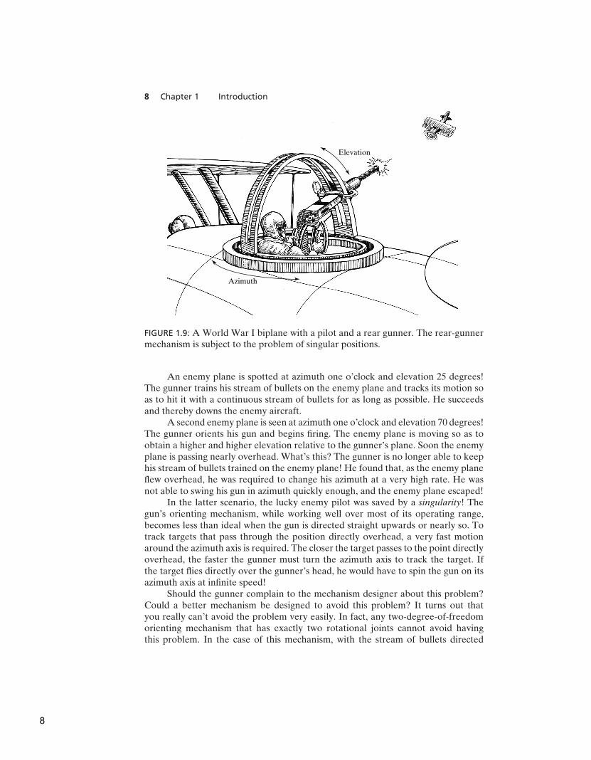
Consider the rear gunner in a World War I–vintage biplane fighter plane(illustrated in Fig. 1.9). While the pilot flies the plane from the front cockpit, the reargunner’s job is to shoot at enemy aircraft. To perform this task, his gun is mountedin a mechanism that rotates about two axes, the motions being called azimuth andelevation. Using these two motions (two degrees of freedom), the gunner can directhis stream of bullets in any direction he desires in the upper hemisphere.
y
�
�1�
�2�
�3�
FIGURE 1.8: The geometrical relationship between joint rates and velocity of theend-effector can be described in a matrix called the Jacobian.
7
8 Chapter 1 Introduction
Elevation
Azimuth
FIGURE 1.9: A World War I biplane with a pilot and a rear gunner. The rear-gunnermechanism is subject to the problem of singular positions.
An enemy plane is spotted at azimuth one o’clock and elevation 25 degrees!The gunner trains his stream of bullets on the enemy plane and tracks its motion soas to hit it with a continuous stream of bullets for as long as possible. He succeedsand thereby downs the enemy aircraft.
A second enemy plane is seen at azimuth one o’clock and elevation 70 degrees!The gunner orients his gun and begins firing. The enemy plane is moving so as toobtain a higher and higher elevation relative to the gunner’s plane. Soon the enemyplane is passing nearly overhead. What’s this? The gunner is no longer able to keephis stream of bullets trained on the enemy plane! He found that, as the enemy planeflew overhead, he was required to change his azimuth at a very high rate. He wasnot able to swing his gun in azimuth quickly enough, and the enemy plane escaped!
In the latter scenario, the lucky enemy pilot was saved by a singularity! Thegun’s orienting mechanism, while working well over most of its operating range,becomes less than ideal when the gun is directed straight upwards or nearly so. Totrack targets that pass through the position directly overhead, a very fast motionaround the azimuth axis is required. The closer the target passes to the point directlyoverhead, the faster the gunner must turn the azimuth axis to track the target. Ifthe target flies directly over the gunner’s head, he would have to spin the gun on itsazimuth axis at infinite speed!
Should the gunner complain to the mechanism designer about this problem?Could a better mechanism be designed to avoid this problem? It turns out thatyou really can’t avoid the problem very easily. In fact, any two-degree-of-freedomorienting mechanism that has exactly two rotational joints cannot avoid havingthis problem. In the case of this mechanism, with the stream of bullets directed
8
Section 1.2 The mechanics and control of mechanical manipulators 9
straight up, their direction aligns with the axis of rotation of the azimuth rotation.This means that, at exactly this point, the azimuth rotation does not cause achange in the direction of the stream of bullets. We know we need two degreesof freedom to orient the stream of bullets, but, at this point, we have lost theeffective use of one of the joints. Our mechanism has become locally degenerateat this location and behaves as if it only has one degree of freedom (the elevationdirection).
This kind of phenomenon is caused by what is called a singularity of themechanism. All mechanisms are prone to these difficulties, including robots. Justas with the rear gunner’s mechanism, these singularity conditions do not preventa robot arm from positioning anywhere within its workspace. However, they cancause problems with motions of the arm in their neighborhood.
Manipulators do not always move through space; sometimes they are alsorequired to touch a workpiece or work surface and apply a static force. In thiscase the problem arises: Given a desired contact force and moment, what set ofjoint torques is required to generate them? Once again, the Jacobian matrix of themanipulator arises quite naturally in the solution of this problem.
Dynamics
Dynamics is a huge field of study devoted to studying the forces required to causemotion. In order to accelerate a manipulator from rest, glide at a constant end-effector velocity, and finally decelerate to a stop, a complex set of torque functionsmust be applied by the joint actuators.2 The exact form of the required functions ofactuator torque depend on the spatial and temporal attributes of the path taken bythe end-effector and on the mass properties of the links and payload, friction in thejoints, and so on. One method of controlling a manipulator to follow a desired pathinvolves calculating these actuator torque functions by using the dynamic equationsof motion of the manipulator.
Many of us have experienced lifting an object that is actually much lighterthan we expected (e.g., getting a container of milk from the refrigerator whichwe thought was full, but was nearly empty). Such a misjudgment of payload cancause an unusual lifting motion. This kind of observation indicates that the humancontrol system is more sophisticated than a purely kinematic scheme. Rather, ourmanipulation control system makes use of knowledge of mass and other dynamiceffects. Likewise, algorithms that we construct to control the motions of a robotmanipulator should take dynamics into account.
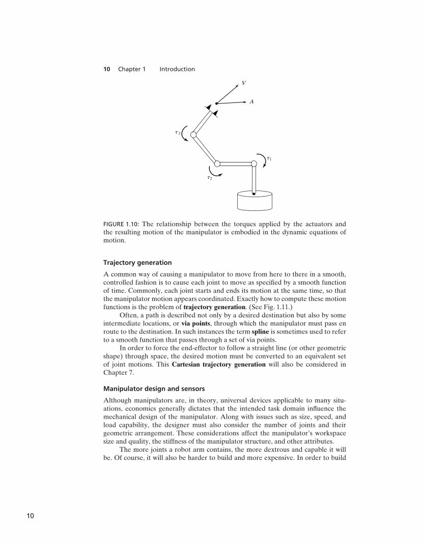
A second use of the dynamic equations of motion is in simulation. By refor-mulating the dynamic equations so that acceleration is computed as a function ofactuator torque, it is possible to simulate how a manipulator would move underapplication of a set of actuator torques. (See Fig. 1.10.) As computing powerbecomes more and more cost effective, the use of simulations is growing in use andimportance in many fields.
In Chapter 6, we develop dynamic equations of motion, which may be used tocontrol or simulate the motion of manipulators.
2We use joint actuators as the generic term for devices that power a manipulator—for example,electric motors, hydraulic and pneumatic actuators, and muscles.
9
10 Chapter 1 Introduction
A
V
t3
t2
t1
FIGURE 1.10: The relationship between the torques applied by the actuators andthe resulting motion of the manipulator is embodied in the dynamic equations ofmotion.
Trajectory generation
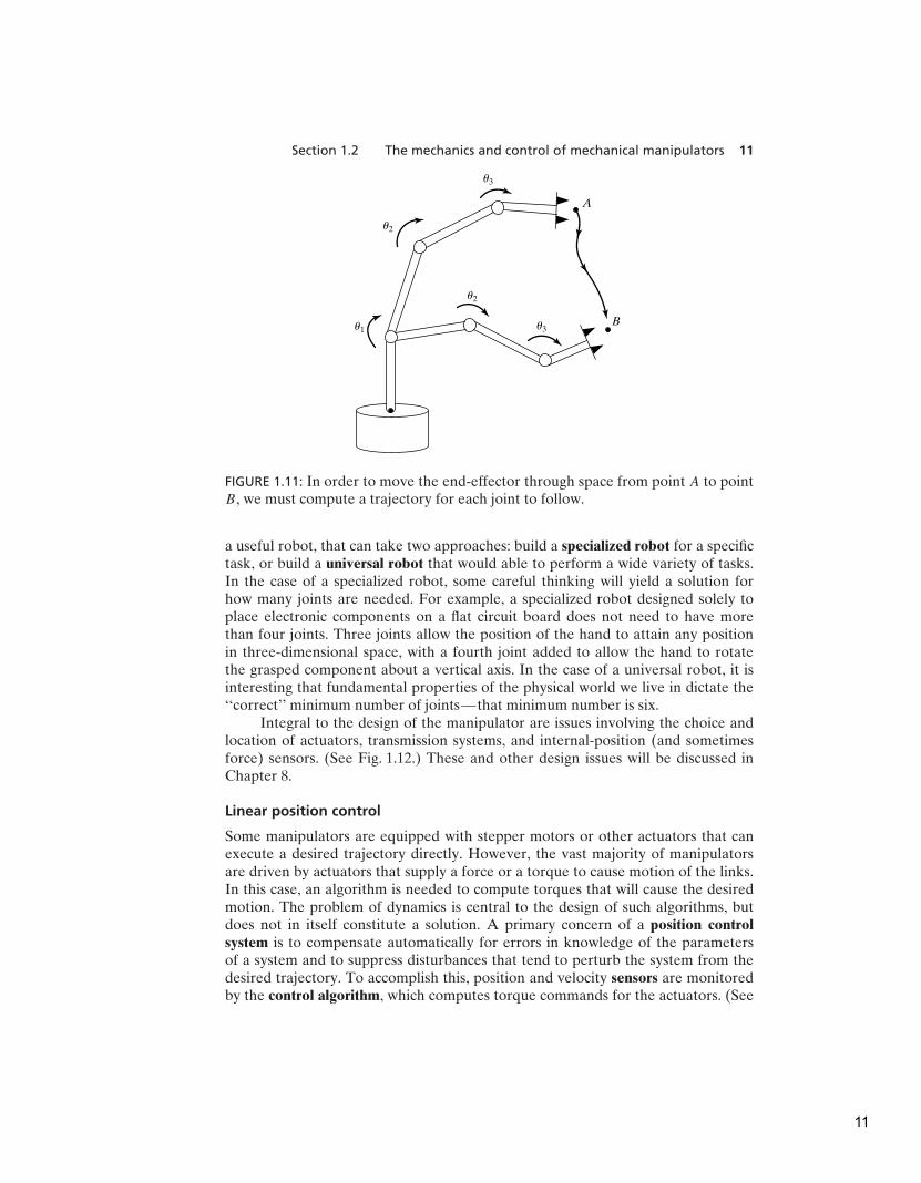
A common way of causing a manipulator to move from here to there in a smooth,controlled fashion is to cause each joint to move as specified by a smooth functionof time. Commonly, each joint starts and ends its motion at the same time, so thatthe manipulator motion appears coordinated. Exactly how to compute these motionfunctions is the problem of trajectory generation. (See Fig. 1.11.)
Often, a path is described not only by a desired destination but also by someintermediate locations, or via points, through which the manipulator must pass enroute to the destination. In such instances the term spline is sometimes used to referto a smooth function that passes through a set of via points.
In order to force the end-effector to follow a straight line (or other geometricshape) through space, the desired motion must be converted to an equivalent setof joint motions. This Cartesian trajectory generation will also be considered inChapter 7.
Manipulator design and sensors
Although manipulators are, in theory, universal devices applicable to many situ-ations, economics generally dictates that the intended task domain influence themechanical design of the manipulator. Along with issues such as size, speed, andload capability, the designer must also consider the number of joints and theirgeometric arrangement. These considerations affect the manipulator’s workspacesize and quality, the stiffness of the manipulator structure, and other attributes.
The more joints a robot arm contains, the more dextrous and capable it willbe. Of course, it will also be harder to build and more expensive. In order to build
10
Section 1.2 The mechanics and control of mechanical manipulators 11
B
A
u2
u1
u3
u2
u3
FIGURE 1.11: In order to move the end-effector through space from point A to pointB, we must compute a trajectory for each joint to follow.
a useful robot, that can take two approaches: build a specialized robot for a specifictask, or build a universal robot that would able to perform a wide variety of tasks.In the case of a specialized robot, some careful thinking will yield a solution forhow many joints are needed. For example, a specialized robot designed solely toplace electronic components on a flat circuit board does not need to have morethan four joints. Three joints allow the position of the hand to attain any positionin three-dimensional space, with a fourth joint added to allow the hand to rotatethe grasped component about a vertical axis. In the case of a universal robot, it isinteresting that fundamental properties of the physical world we live in dictate the‘‘correct’’ minimum number of joints—that minimum number is six.
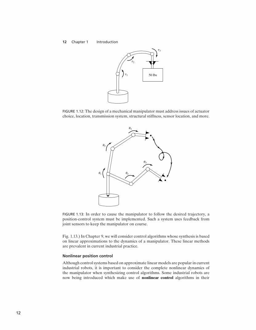
Integral to the design of the manipulator are issues involving the choice andlocation of actuators, transmission systems, and internal-position (and sometimesforce) sensors. (See Fig. 1.12.) These and other design issues will be discussed inChapter 8.
Linear position control
Some manipulators are equipped with stepper motors or other actuators that canexecute a desired trajectory directly. However, the vast majority of manipulatorsare driven by actuators that supply a force or a torque to cause motion of the links.In this case, an algorithm is needed to compute torques that will cause the desiredmotion. The problem of dynamics is central to the design of such algorithms, butdoes not in itself constitute a solution. A primary concern of a position controlsystem is to compensate automatically for errors in knowledge of the parametersof a system and to suppress disturbances that tend to perturb the system from thedesired trajectory. To accomplish this, position and velocity sensors are monitoredby the control algorithm, which computes torque commands for the actuators. (See
11
12 Chapter 1 Introduction
t3
t2
t1 50 lbs
FIGURE 1.12: The design of a mechanical manipulator must address issues of actuatorchoice, location, transmission system, structural stiffness, sensor location, and more.
u2
u3
u1 u2
u3
FIGURE 1.13: In order to cause the manipulator to follow the desired trajectory, aposition-control system must be implemented. Such a system uses feedback fromjoint sensors to keep the manipulator on course.
Fig. 1.13.) In Chapter 9, we will consider control algorithms whose synthesis is basedon linear approximations to the dynamics of a manipulator. These linear methodsare prevalent in current industrial practice.
Nonlinear position control
Although control systems based on approximate linear models are popular in currentindustrial robots, it is important to consider the complete nonlinear dynamics ofthe manipulator when synthesizing control algorithms. Some industrial robots arenow being introduced which make use of nonlinear control algorithms in their
12

Section 1.2 The mechanics and control of mechanical manipulators 13
controllers. These nonlinear techniques of controlling a manipulator promise betterperformance than do simpler linear schemes. Chapter 10 will introduce nonlinearcontrol systems for mechanical manipulators.
Force control
The ability of a manipulator to control forces of contact when it touches parts,tools, or work surfaces seems to be of great importance in applying manipulatorsto many real-world tasks. Force control is complementary to position control, inthat we usually think of only one or the other as applicable in a certain situation.When a manipulator is moving in free space, only position control makes sense,because there is no surface to react against. When a manipulator is touching arigid surface, however, position-control schemes can cause excessive forces to buildup at the contact or cause contact to be lost with the surface when it was desiredfor some application. Manipulators are rarely constrained by reaction surfaces inall directions simultaneously, so a mixed or hybrid control is required, with somedirections controlled by a position-control law and remaining directions controlledby a force-control law. (See Fig. 1.14.) Chapter 11 introduces a methodology forimplementing such a force-control scheme.
A robot should be instructed to wash a window by maintaining a certainforce in the direction perpendicular to the plane of the glass, while following amotion trajectory in directions tangent to the plane. Such split or hybrid controlspecifications are natural for such tasks.
Programming robots
A robot programming language serves as the interface between the human userand the industrial robot. Central questions arise: How are motions through spacedescribed easily by the programmer? How are multiple manipulators programmed
V
F
F
FIGURE 1.14: In order for a manipulator to slide across a surface while applying aconstant force, a hybrid position–force control system must be used.
13
14 Chapter 1 Introduction
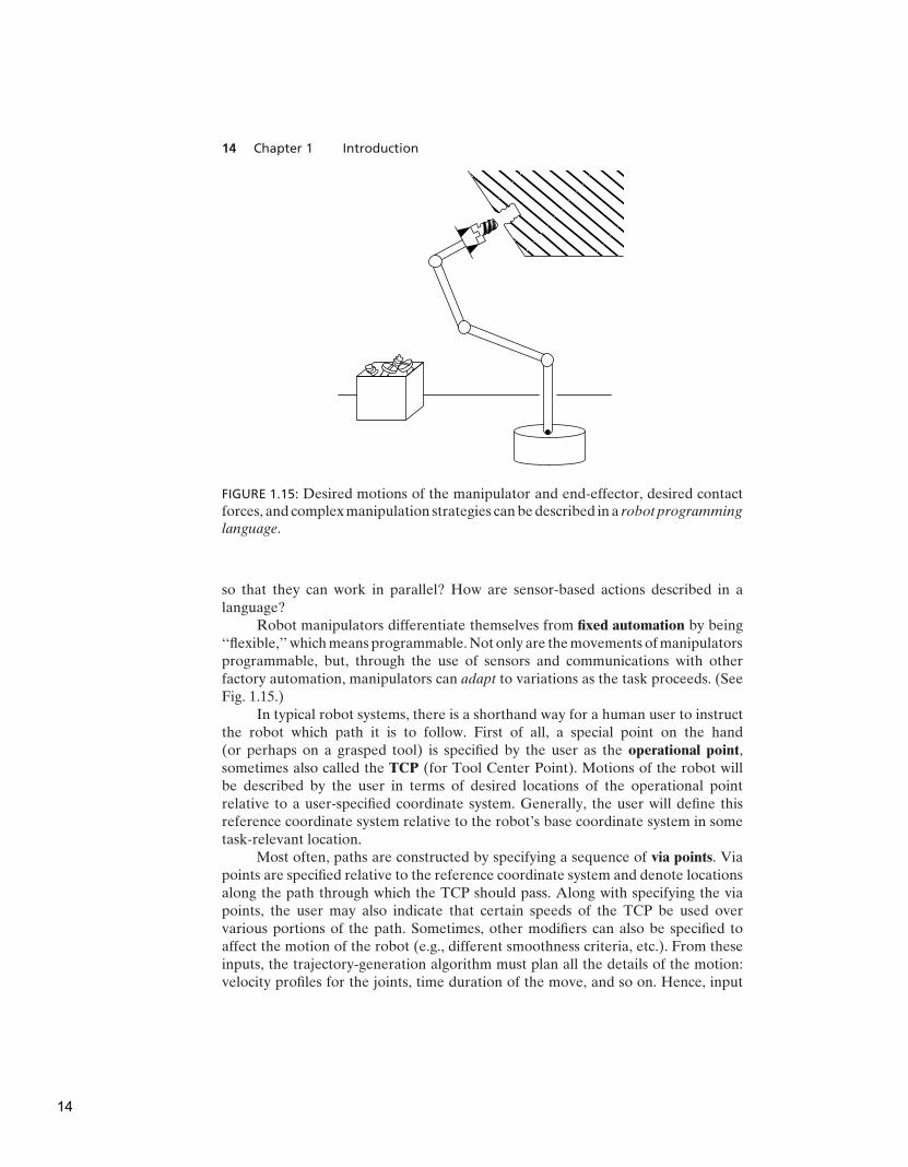
FIGURE 1.15: Desired motions of the manipulator and end-effector, desired contactforces, and complex manipulation strategies can be described in a robot programming
language.
so that they can work in parallel? How are sensor-based actions described in alanguage?
Robot manipulators differentiate themselves from fixed automation by being‘‘flexible,’’ which means programmable. Not only are the movements of manipulatorsprogrammable, but, through the use of sensors and communications with otherfactory automation, manipulators can adapt to variations as the task proceeds. (SeeFig. 1.15.)
In typical robot systems, there is a shorthand way for a human user to instructthe robot which path it is to follow. First of all, a special point on the hand(or perhaps on a grasped tool) is specified by the user as the operational point,sometimes also called the TCP (for Tool Center Point). Motions of the robot willbe described by the user in terms of desired locations of the operational pointrelative to a user-specified coordinate system. Generally, the user will define thisreference coordinate system relative to the robot’s base coordinate system in sometask-relevant location.
Most often, paths are constructed by specifying a sequence of via points. Viapoints are specified relative to the reference coordinate system and denote locationsalong the path through which the TCP should pass. Along with specifying the viapoints, the user may also indicate that certain speeds of the TCP be used overvarious portions of the path. Sometimes, other modifiers can also be specified toaffect the motion of the robot (e.g., different smoothness criteria, etc.). From theseinputs, the trajectory-generation algorithm must plan all the details of the motion:velocity profiles for the joints, time duration of the move, and so on. Hence, input
14

Section 1.2 The mechanics and control of mechanical manipulators 15
to the trajectory-generation problem is generally given by constructs in the robotprogramming language.
The sophistication of the user interface is becoming extremely importantas manipulators and other programmable automation are applied to more andmore demanding industrial applications. The problem of programming manipu-lators encompasses all the issues of ‘‘traditional’’ computer programming and sois an extensive subject in itself. Additionally, some particular attributes of themanipulator-programming problem cause additional issues to arise. Some of thesetopics will be discussed in Chapter 12.
Off-line programming and simulation
An off-line programming system is a robot programming environment that hasbeen sufficiently extended, generally by means of computer graphics, that thedevelopment of robot programs can take place without access to the robot itself. Acommon argument raised in their favor is that an off-line programming system willnot cause production equipment (i.e., the robot) to be tied up when it needs to bereprogrammed; hence, automated factories can stay in production mode a greaterpercentage of the time. (See Fig. 1.16.)
They also serve as a natural vehicle to tie computer-aided design (CAD) databases used in the design phase of a product to the actual manufacturing of theproduct. In some cases, this direct use of CAD data can dramatically reduce theprogramming time required for the manufacturing process. Chapter 13 discusses theelements of industrial robot off-line programming systems.
FIGURE 1.16: Off-line programming systems, generally providing a computer graphicsinterface, allow robots to be programmed without access to the robot itself duringprogramming.
15
16 Chapter 1 Introduction
1.3 NOTATION
Notation is always an issue in science and engineering. In this book, we use thefollowing conventions:
1. Usually, variables written in uppercase represent vectors or matrices. Lower-case variables are scalars.
2. Leading subscripts and superscripts identify which coordinate system a quantityis written in. For example, AP represents a position vector written in coordinatesystem {A}, and A
BR is a rotation matrix3 that specifies the relationship between
coordinate systems {A} and {B}.
3. Trailing superscripts are used (as widely accepted) for indicating the inverseor transpose of a matrix (e.g., R−1, RT ).
4. Trailing subscripts are not subject to any strict convention but may indicate avector component (e.g., x, y, or z) or may be used as a description—as in Pbolt ,the position of a bolt.
5. We will use many trigonometric functions. Our notation for the cosine of anangle θ1 may take any of the following forms: cos θ1 = cθ1 = c1.
Vectors are taken to be column vectors; hence, row vectors will have thetranspose indicated explicitly.
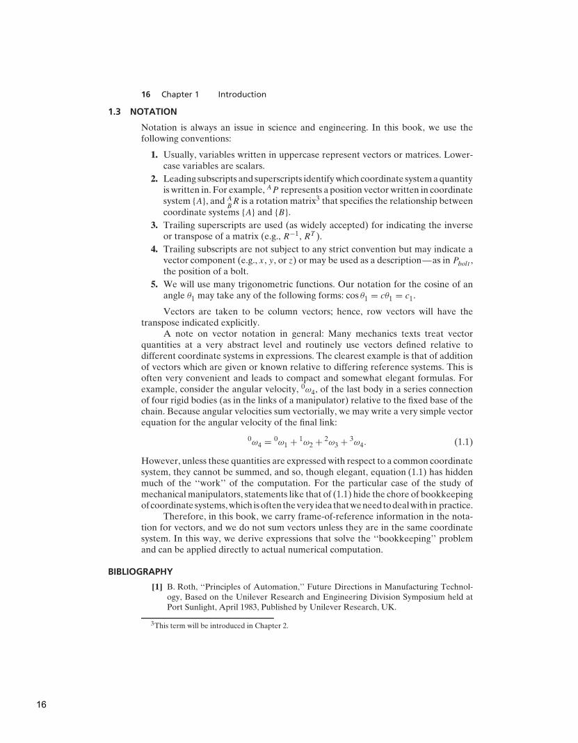
A note on vector notation in general: Many mechanics texts treat vectorquantities at a very abstract level and routinely use vectors defined relative todifferent coordinate systems in expressions. The clearest example is that of additionof vectors which are given or known relative to differing reference systems. This isoften very convenient and leads to compact and somewhat elegant formulas. Forexample, consider the angular velocity, 0ω4, of the last body in a series connectionof four rigid bodies (as in the links of a manipulator) relative to the fixed base of thechain. Because angular velocities sum vectorially, we may write a very simple vectorequation for the angular velocity of the final link:
0ω4 = 0ω1 + 1ω2 + 2ω3 + 3ω4. (1.1)
However, unless these quantities are expressed with respect to a common coordinatesystem, they cannot be summed, and so, though elegant, equation (1.1) has hiddenmuch of the ‘‘work’’ of the computation. For the particular case of the study ofmechanical manipulators, statements like that of (1.1) hide the chore of bookkeepingofcoordinatesystems, which isoftenthevery ideathatweneedtodealwith in practice.
Therefore, in this book, we carry frame-of-reference information in the nota-tion for vectors, and we do not sum vectors unless they are in the same coordinatesystem. In this way, we derive expressions that solve the ‘‘bookkeeping’’ problemand can be applied directly to actual numerical computation.
BIBLIOGRAPHY
[1] B. Roth, ‘‘Principles of Automation,’’ Future Directions in Manufacturing Technol-ogy, Based on the Unilever Research and Engineering Division Symposium held atPort Sunlight, April 1983, Published by Unilever Research, UK.
3This term will be introduced in Chapter 2.
16

Exercises 17
[2] R. Brooks, ‘‘Flesh and Machines,’’ Pantheon Books, New York, 2002.
[3] The International Federation of Robotics, and the United Nations, ‘‘World Robotics2001,’’ Statistics, Market Analysis, Forecasts, Case Studies and Profitability of RobotInvestment, United Nations Publication, New York and Geneva, 2001.
General-reference books
[4] R. Paul, Robot Manipulators, MIT Press, Cambridge, MA, 1981.
[5] M. Brady et al., Robot Motion, MIT Press, Cambridge, MA, 1983.
[6] W. Synder, Industrial Robots: Computer Interfacing and Control, Prentice-Hall, Engle-wood Cliffs, NJ, 1985.
[7] Y. Koren, Robotics for Engineers, McGraw-Hill, New York, 1985.
[8] H. Asada and J.J. Slotine, Robot Analysis and Control, Wiley, New York, 1986.
[9] K. Fu, R. Gonzalez, and C.S.G. Lee, Robotics: Control, Sensing, Vision, and Intelli-
gence, McGraw-Hill, New York, 1987.
[10] E. Riven, Mechanical Design of Robots, McGraw-Hill, New York, 1988.
[11] J.C. Latombe, Robot Motion Planning, Kluwer Academic Publishers, Boston, 1991.
[12] M. Spong, Robot Control: Dynamics, Motion Planning, and Analysis, IEEE Press,New York, 1992.
[13] S.Y. Nof, Handbook of Industrial Robotics, 2nd Edition, Wiley, New York, 1999.
[14] L.W. Tsai, Robot Analysis: The Mechanics of Serial and Parallel Manipulators, Wiley,New York, 1999.
[15] L. Sciavicco and B. Siciliano, Modelling and Control of Robot Manipulators, 2ndEdition, Springer-Verlag, London, 2000.
[16] G. Schmierer and R. Schraft, Service Robots, A.K. Peters, Natick, MA, 2000.
General-reference journals and magazines
[17] Robotics World.
[18] IEEE Transactions on Robotics and Automation.
[19] International Journal of Robotics Research (MIT Press).
[20] ASME Journal of Dynamic Systems, Measurement, and Control.
[21] International Journal of Robotics & Automation (IASTED).
EXERCISES
1.1 [20] Make a chronology of major events in the development of industrial robotsover the past 40 years. See Bibliography and general references.
1.2 [20] Make a chart showing the major applications of industrial robots (e.g., spotwelding, assembly, etc.) and the percentage of installed robots in use in eachapplication area. Base your chart on the most recent data you can find. SeeBibliography and general references.
1.3 [40] Figure 1.3 shows how the cost of industrial robots has declined over the years.Find data on the cost of human labor in various specific industries (e.g., labor inthe auto industry, labor in the electronics assembly industry, labor in agriculture,etc.) and create a graph showing how these costs compare to the use of robotics.You should see that the robot cost curve ‘‘crosses’’ various the human cost curves
17
18 Chapter 1 Introduction
of different industries at different times. From this, derive approximate dateswhen robotics first became cost effective for use in various industries.
1.4 [10] In a sentence or two, define kinematics, workspace, and trajectory.1.5 [10] In a sentence or two, define frame, degree of freedom, and position control.1.6 [10] In a sentence or two, define force control, and robot programming language.1.7 [10] In a sentence or two, define nonlinear control, and off-line programming.1.8 [20] Make a chart indicating how labor costs have risen over the past 20 years.1.9 [20] Make a chart indicating how the computer performance–price ratio has
increased over the past 20 years.1.10 [20] Make a chart showing the major users of industrial robots (e.g., aerospace,
automotive, etc.) and the percentage of installed robots in use in each industry.Base your chart on the most recent data you can find. (See reference section.)
PROGRAMMING EXERCISE (PART 1)
Familiarize yourself with the computer you will use to do the programming exercises atthe end of each chapter. Make sure you can create and edit files and can compile andexecute programs.
MATLAB EXERCISE 1
At the end of most chapters in this textbook, a MATLAB exercise is given. Generally,these exercises ask the student to program the pertinent robotics mathematics inMATLAB and then check the results of the MATLAB Robotics Toolbox. The textbookassumes familiarity with MATLAB and linear algebra (matrix theory). Also, the studentmust become familiar with the MATLAB Robotics Toolbox. For MATLAB Exercise 1,
a) Familiarize yourself with the MATLAB programming environment if necessary. Atthe MATLAB software prompt, try typing demo and help. Using the color-codedMATLAB editor, learn how to create, edit, save, run, and debug m-files (ASCIIfiles with series of MATLAB statements). Learn how to create arrays (matrices andvectors), and explore the built-in MATLAB linear-algebra functions for matrixand vector multiplication, dot and cross products, transposes, determinants, andinverses, and for the solution of linear equations. MATLAB is based on thelanguage C, but is generally much easier to use. Learn how to program logicalconstructs and loops in MATLAB. Learn how to use subprograms and functions.Learn how to use comments (%) for explaining your programs and tabs for easyreadability. Check out www.mathworks.com for more information and tutorials.Advanced MATLAB users should become familiar with Simulink, the graphicalinterface of MATLAB, and with the MATLAB Symbolic Toolbox.
b) Familiarize yourself with the MATLAB Robotics Toolbox, a third-party toolboxdeveloped by Peter I. Corke of CSIRO, Pinjarra Hills, Australia. This productcan be downloaded for free from www.cat.csiro.au/cmst/staff/pic/robot. The sourcecode is readable and changeable, and there is an international community ofusers, at [email protected]. Download the MATLAB RoboticsToolbox, and install it on your computer by using the .zip file and following theinstructions. Read the README file, and familiarize yourself with the variousfunctions available to the user. Find the robot.pdf file—this is the user manualgiving background information and detailed usage of all of the Toolbox functions.Don’t worry if you can’t understand the purpose of these functions yet; they dealwith robotics mathematics concepts covered in Chapters 2 through 7 of this book.
18
C H A P T E R 2
Spatial descriptionsand transformations
2.1 INTRODUCTION
2.2 DESCRIPTIONS: POSITIONS, ORIENTATIONS, AND FRAMES
2.3 MAPPINGS: CHANGING DESCRIPTIONS FROM FRAME TO FRAME
2.4 OPERATORS: TRANSLATIONS, ROTATIONS, AND TRANSFORMATIONS
2.5 SUMMARY OF INTERPRETATIONS
2.6 TRANSFORMATION ARITHMETIC
2.7 TRANSFORM EQUATIONS
2.8 MORE ON REPRESENTATION OF ORIENTATION
2.9 TRANSFORMATION OF FREE VECTORS
2.10 COMPUTATIONAL CONSIDERATIONS
2.1 INTRODUCTION
Robotic manipulation, by definition, implies that parts and tools will be movedaround in space by some sort of mechanism. This naturally leads to a need forrepresenting positions and orientations of parts, of tools, and of the mechanismitself. To define and manipulate mathematical quantities that represent positionand orientation, we must define coordinate systems and develop conventions forrepresentation. Many of the ideas developed here in the context of position andorientation will form a basis for our later consideration of linear and rotationalvelocities, forces, and torques.
We adopt the philosophy that somewhere there is a universe coordinate systemto which everything we discuss can be referenced. We will describe all positionsand orientations with respect to the universe coordinate system or with respect toother Cartesian coordinate systems that are (or could be) defined relative to theuniverse system.
2.2 DESCRIPTIONS: POSITIONS, ORIENTATIONS, AND FRAMES
A description is used to specify attributes of various objects with which a manipula-tion system deals. These objects are parts, tools, and the manipulator itself. In thissection, we discuss the description of positions, of orientations, and of an entity thatcontains both of these descriptions: the frame.
From Chapter 2 of Introduction to Robotics: Mechanics and Control, Third Edition. John J. Craig.
Copyright © 2005 by Pearson Education, Inc. All rights reserved.
19
20 Chapter 2 Spatial descriptions and transformations
Description of a position
Once a coordinate system is established, we can locate any point in the universe witha 3 × 1 position vector. Because we will often define many coordinate systems inaddition to the universe coordinate system, vectors must be tagged with informationidentifying which coordinate system they are defined within. In this book, vectorsare written with a leading superscript indicating the coordinate system to whichthey are referenced (unless it is clear from context)—for example, AP . This meansthat the components of AP have numerical values that indicate distances along theaxes of {A}. Each of these distances along an axis can be thought of as the result ofprojecting the vector onto the corresponding axis.
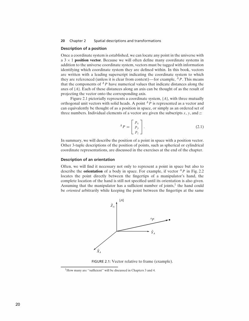
Figure 2.1 pictorially represents a coordinate system, {A}, with three mutuallyorthogonal unit vectors with solid heads. A point AP is represented as a vector andcan equivalently be thought of as a position in space, or simply as an ordered set ofthree numbers. Individual elements of a vector are given the subscripts x, y, and z:
AP =
pxpypz
. (2.1)
In summary, we will describe the position of a point in space with a position vector.Other 3-tuple descriptions of the position of points, such as spherical or cylindricalcoordinate representations, are discussed in the exercises at the end of the chapter.
Description of an orientation
Often, we will find it necessary not only to represent a point in space but also todescribe the orientation of a body in space. For example, if vector AP in Fig. 2.2locates the point directly between the fingertips of a manipulator’s hand, thecomplete location of the hand is still not specified until its orientation is also given.Assuming that the manipulator has a sufficient number of joints,1 the hand couldbe oriented arbitrarily while keeping the point between the fingertips at the same
AP
YA
ZA
XA
{A}
FIGURE 2.1: Vector relative to frame (example).
1How many are ‘‘sufficient’’ will be discussed in Chapters 3 and 4.
20
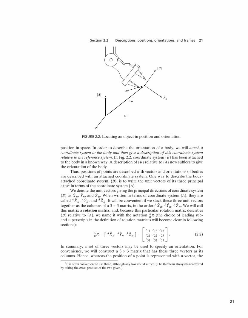
Section 2.2 Descriptions: positions, orientations, and frames 21
AP
ZB
{A}
{B}
FIGURE 2.2: Locating an object in position and orientation.
position in space. In order to describe the orientation of a body, we will attach a
coordinate system to the body and then give a description of this coordinate system
relative to the reference system. In Fig. 2.2, coordinate system {B} has been attachedto the body in a known way. A description of {B} relative to {A} now suffices to givethe orientation of the body.
Thus, positions of points are described with vectors and orientations of bodiesare described with an attached coordinate system. One way to describe the body-attached coordinate system, {B}, is to write the unit vectors of its three principalaxes2 in terms of the coordinate system {A}.
We denote the unit vectors giving the principal directions of coordinate system{B} as XB , YB , and ZB . When written in terms of coordinate system {A}, they are
called AXB , AYB , and AZB . It will be convenient if we stack these three unit vectors
together as the columns of a 3 × 3 matrix, in the order AXB , AYB , AZB . We will callthis matrix a rotation matrix, and, because this particular rotation matrix describes{B} relative to {A}, we name it with the notation A
BR (the choice of leading sub-
and superscripts in the definition of rotation matrices will become clear in followingsections):
A
BR =
[
AXBAYB
AZB
]
=
r11 r12 r13r21 r22 r23r31 r32 r33
. (2.2)
In summary, a set of three vectors may be used to specify an orientation. Forconvenience, we will construct a 3 × 3 matrix that has these three vectors as itscolumns. Hence, whereas the position of a point is represented with a vector, the
2It is often convenient to use three, although any two would suffice. (The third can always be recoveredby taking the cross product of the two given.)
21
22 Chapter 2 Spatial descriptions and transformations
orientation of a body is represented with a matrix. In Section 2.8, we will considersome other descriptions of orientation that require only three parameters.
We can give expressions for the scalars rij in (2.2) by noting that the componentsof any vector are simply the projections of that vector onto the unit directions of itsreference frame. Hence, each component of A
BR in (2.2) can be written as the dot
product of a pair of unit vectors:
A
BR =
[
AXBAYB
AZB
]
=
XB · XA YB · XA ZB · XA
XB · YA YB · YA ZB · YAXB · ZA YB · ZA ZB · ZA
. (2.3)
For brevity, we have omitted the leading superscripts in the rightmost matrix of(2.3). In fact, the choice of frame in which to describe the unit vectors is arbitrary aslong as it is the same for each pair being dotted. The dot product of two unit vectorsyields the cosine of the angle between them, so it is clear why the components ofrotation matrices are often referred to as direction cosines.
Further inspection of (2.3) shows that the rows of the matrix are the unitvectors of {A} expressed in {B}; that is,
A
BR =
[
AXBAYB
AZB
]
=
BXTA
B Y TA
BZTA
. (2.4)
Hence, BAR, the description of frame {A} relative to {B}, is given by the transpose of
(2.3); that is,B
AR = A
BRT . (2.5)
This suggests that the inverse of a rotation matrix is equal to its transpose, a factthat can be easily verified as
A
BRT A
BR =
AXTB
AY TB
AZTB
[
AXBAYB
AZB
]
= I3, (2.6)
where I3 is the 3 × 3 identity matrix. Hence,
A
BR = B
AR−1 = B
ART . (2.7)
Indeed, from linear algebra [1], we know that the inverse of a matrix withorthonormal columns is equal to its transpose. We have just shown this geometrically.
Description of a frame
The information needed to completely specify the whereabouts of the manipulatorhand in Fig. 2.2 is a position and an orientation. The point on the body whoseposition we describe could be chosen arbitrarily, however. For convenience, the
22

Section 2.2 Descriptions: positions, orientations, and frames 23
point whose position we will describe is chosen as the origin of the body-attached
frame. The situation of a position and an orientation pair arises so often in roboticsthat we define an entity called a frame, which is a set of four vectors giving positionand orientation information. For example, in Fig. 2.2, one vector locates the fingertipposition and three more describe its orientation. Equivalently, the description of aframe can be thought of as a position vector and a rotation matrix. Note that a frameis a coordinate system where, in addition to the orientation, we give a position vectorwhich locates its origin relative to some other embedding frame. For example, frame{B} is described by A
BR and APBORG, where APBORG is the vector that locates the
origin of the frame {B}:{B} = {A
BR,A PBORG}. (2.8)
In Fig. 2.3, there are three frames that are shown along with the universe coordinatesystem. Frames {A} and {B} are known relative to the universe coordinate system,and frame {C} is known relative to frame {A}.
In Fig. 2.3, we introduce a graphical representation of frames, which is conve-nient in visualizing frames. A frame is depicted by three arrows representing unitvectors defining the principal axes of the frame. An arrow representing a vector isdrawn from one origin to another. This vector represents the position of the originat the head of the arrow in terms of the frame at the tail of the arrow. The directionof this locating arrow tells us, for example, in Fig. 2.3, that {C} is known relative to{A} and not vice versa.
In summary, a frame can be used as a description of one coordinate systemrelative to another. A frame encompasses two ideas by representing both positionand orientation and so may be thought of as a generalization of those two ideas.Positions could be represented by a frame whose rotation-matrix part is the identitymatrix and whose position-vector part locates the point being described. Likewise,an orientation could be represented by a frame whose position-vector part was thezero vector.
ZU
ZB
ZA
ZC
XC
YC
YA
YU
XU XB
YB
XA
{U}
{B}
{C}
{A}
FIGURE 2.3: Example of several frames.
23

24 Chapter 2 Spatial descriptions and transformations
2.3 MAPPINGS: CHANGING DESCRIPTIONS FROM FRAME TO FRAME
In a great many of the problems in robotics, we are concerned with expressing thesame quantity in terms of various reference coordinate systems. The previous sectionintroduced descriptions of positions, orientations, and frames; we now consider themathematics of mapping in order to change descriptions from frame to frame.
Mappings involving translated frames
In Fig. 2.4, we have a position defined by the vector BP . We wish to express thispoint in space in terms of frame {A}, when {A} has the same orientation as {B}. Inthis case, {B} differs from {A} only by a translation, which is given by APBORG, avector that locates the origin of {B} relative to {A}.
Because both vectors are defined relative to frames of the same orientation,we calculate the description of point P relative to {A}, AP , by vector addition:
AP = BP + APBORG. (2.9)
Note that only in the special case of equivalent orientations may we add vectors thatare defined in terms of different frames.
In this simple example, we have illustrated mapping a vector from one frameto another. This idea of mapping, or changing the description from one frame toanother, is an extremely important concept. The quantity itself (here, a point inspace) is not changed; only its description is changed. This is illustrated in Fig. 2.4,where the point described by BP is not translated, but remains the same, and insteadwe have computed a new description of the same point, but now with respect tosystem {A}.
AP
BP
APBORG
YA
ZA
XA
{A}
YB
ZB
XB
{B}
FIGURE 2.4: Translational mapping.
24

Section 2.3 Mappings: changing descriptions from frame to frame 25
We say that the vector APBORG defines this mapping because all the informa-tion needed to perform the change in description is contained in APBORG (alongwith the knowledge that the frames had equivalent orientation).
Mappings involving rotated frames
Section 2.2 introduced the notion of describing an orientation by three unit vectorsdenoting the principal axes of a body-attached coordinate system. For convenience,we stack these three unit vectors together as the columns of a 3 × 3 matrix. We willcall this matrix a rotation matrix, and, if this particular rotation matrix describes {B}relative to {A}, we name it with the notation A
BR.
Note that, by our definition, the columns of a rotation matrix all have unitmagnitude, and, further, that these unit vectors are orthogonal. As we saw earlier, aconsequence of this is that
A
BR = B
AR−1 = B
ART . (2.10)
Therefore, because the columns of ABR are the unit vectors of {B} written in {A}, the
rows of ABR are the unit vectors of {A} written in {B}.
So a rotation matrix can be interpreted as a set of three column vectors or as aset of three row vectors, as follows:
A
BR =
[
AXBAYB
AZB
]
=
BXTA
B Y TA
BZTA
. (2.11)
As in Fig. 2.5, the situation will arise often where we know the definition of a vectorwith respect to some frame, {B}, and we would like to know its definition withrespect to another frame, {A}, where the origins of the two frames are coincident.
BP
YA
YB
ZA
XB
ZB
XA
{A}{B}
FIGURE 2.5: Rotating the description of a vector.
25
26 Chapter 2 Spatial descriptions and transformations
This computation is possible when a description of the orientation of {B} is knownrelative to {A}. This orientation is given by the rotation matrix A
BR, whose columns
are the unit vectors of {B} written in {A}.In order to calculate AP , we note that the components of any vector are simply
the projections of that vector onto the unit directions of its frame. The projection iscalculated as the vector dot product. Thus, we see that the components of AP maybe calculated as
Apx = BXA · BP,Apy = B YA · BP, (2.12)
Apz = BZA · BP.
In order to express (2.13) in terms of a rotation matrix multiplication, we notefrom (2.11) that the rows of A
BR are BXA, B YA, and BZA. So (2.13) may be written
compactly, by using a rotation matrix, as
AP = A
BR BP. (2.13)
Equation 2.13 implements a mapping—that is, it changes the description of avector—from BP , which describes a point in space relative to {B}, into AP , which isa description of the same point, but expressed relative to {A}.
We now see that our notation is of great help in keeping track of mappingsand frames of reference. A helpful way of viewing the notation we have introducedis to imagine that leading subscripts cancel the leading superscripts of the followingentity, for example the Bs in (2.13).
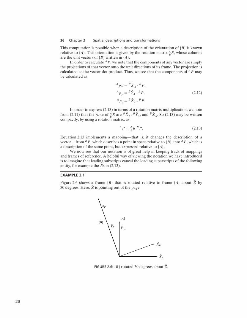
EXAMPLE 2.1
Figure 2.6 shows a frame {B} that is rotated relative to frame {A} about Z by30 degrees. Here, Z is pointing out of the page.
BP
XA
YAYB
XB
{A}{B}
FIGURE 2.6: {B} rotated 30 degrees about Z.
26

Section 2.3 Mappings: changing descriptions from frame to frame 27
Writing the unit vectors of {B} in terms of {A} and stacking them as the columnsof the rotation matrix, we obtain
A
BR =
0.866 −0.500 0.0000.500 0.866 0.0000.000 0.000 1.000
. (2.14)
Given
BP =
0.02.00.0
, (2.15)
we calculate AP as
AP = A
BR BP =
−1.0001.7320.000
. (2.16)
Here, ABR acts as a mapping that is used to describe BP relative to frame {A},
AP . As was introduced in the case of translations, it is important to remember that,viewed as a mapping, the original vector P is not changed in space. Rather, wecompute a new description of the vector relative to another frame.
Mappings involving general frames
Very often, we know the description of a vector with respect to some frame {B}, andwe would like to know its description with respect to another frame, {A}. We nowconsider the general case of mapping. Here, the origin of frame {B} is not coincidentwith that of frame {A} but has a general vector offset. The vector that locates {B}’sorigin is called APBORG. Also {B} is rotated with respect to {A}, as described by A
BR.
Given BP , we wish to compute AP , as in Fig. 2.7.
APBP
APBORG
YA
ZA
XA
{A}
YB
ZB
XB
{B}
FIGURE 2.7: General transform of a vector.
27

28 Chapter 2 Spatial descriptions and transformations
We can first change BP to its description relative to an intermediate framethat has the same orientation as {A}, but whose origin is coincident with the originof {B}. This is done by premultiplying by A
BR as in the last section. We then account
for the translation between origins by simple vector addition, as before, and obtain
AP = A
BR BP + APBORG. (2.17)
Equation 2.17 describes a general transformation mapping of a vector from itsdescription in one frame to a description in a second frame. Note the followinginterpretation of our notation as exemplified in (2.17): the B’s cancel, leaving allquantities as vectors written in terms of A, which may then be added.
The form of (2.17) is not as appealing as the conceptual form
AP = A
BT BP. (2.18)
That is, we would like to think of a mapping from one frame to another as anoperator in matrix form. This aids in writing compact equations and is conceptuallyclearer than (2.17). In order that we may write the mathematics given in (2.17) inthe matrix operator form suggested by (2.18), we define a 4 × 4 matrix operator anduse 4 × 1 position vectors, so that (2.18) has the structure
[
AP
1
]
=[
ABR APBORG
0 0 0 1
]
[
BP
1
]
. (2.19)
In other words,
1. a ‘‘1’’ is added as the last element of the 4 × 1 vectors;
2. a row ‘‘[0 0 0 1]’’ is added as the last row of the 4 × 4 matrix.
We adopt the convention that a position vector is 3 × 1 or 4 × 1, depending onwhether it appears multiplied by a 3 × 3 matrix or by a 4 × 4 matrix. It is readilyseen that (2.19) implements
AP = A
BR BP + APBORG
1 = 1. (2.20)
The 4×4 matrix in (2.19) is called a homogeneous transform. For our purposes,it can be regarded purely as a construction used to cast the rotation and translationof the general transform into a single matrix form. In other fields of study, it can beused to compute perspective and scaling operations (when the last row is other than‘‘[0 0 0 1]’’ or the rotation matrix is not orthonormal). The interested reader shouldsee [2].
Often, we will write an equation like (2.18) without any notation indicatingthat it is a homogeneous representation, because it is obvious from context. Notethat, although homogeneous transforms are useful in writing compact equations, acomputer program to transform vectors would generally not use them, because oftime wasted multiplying ones and zeros. Thus, this representation is mainly for ourconvenience when thinking and writing equations down on paper.
28
Section 2.3 Mappings: changing descriptions from frame to frame 29
Just as we used rotation matrices to specify an orientation, we will usetransforms (usually in homogeneous representation) to specify a frame. Observethat, although we have introduced homogeneous transforms in the context ofmappings, they also serve as descriptions of frames. The description of frame {B}relative to {A} is A
BT .
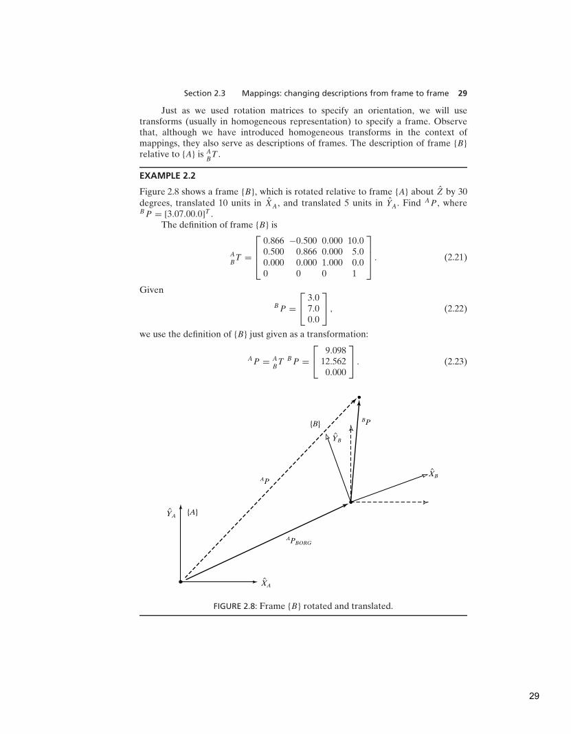
EXAMPLE 2.2
Figure 2.8 shows a frame {B}, which is rotated relative to frame {A} about Z by 30degrees, translated 10 units in XA, and translated 5 units in YA. Find AP , whereBP = [3.07.00.0]T .
The definition of frame {B} is
A
BT =
0.866 −0.500 0.000 10.00.500 0.866 0.000 5.00.000 0.000 1.000 0.00 0 0 1
. (2.21)
Given
BP =
3.07.00.0
, (2.22)
we use the definition of {B} just given as a transformation:
AP = A
BT BP =
9.09812.5620.000
. (2.23)
AP
BP
APBORG
XA
YA{A}
YB
XB
{B}
FIGURE 2.8: Frame {B} rotated and translated.
29
30 Chapter 2 Spatial descriptions and transformations
2.4 OPERATORS: TRANSLATIONS, ROTATIONS, AND TRANSFORMATIONS
The same mathematical forms used to map points between frames can also beinterpreted as operators that translate points, rotate vectors, or do both. This sectionillustrates this interpretation of the mathematics we have already developed.
Translational operators
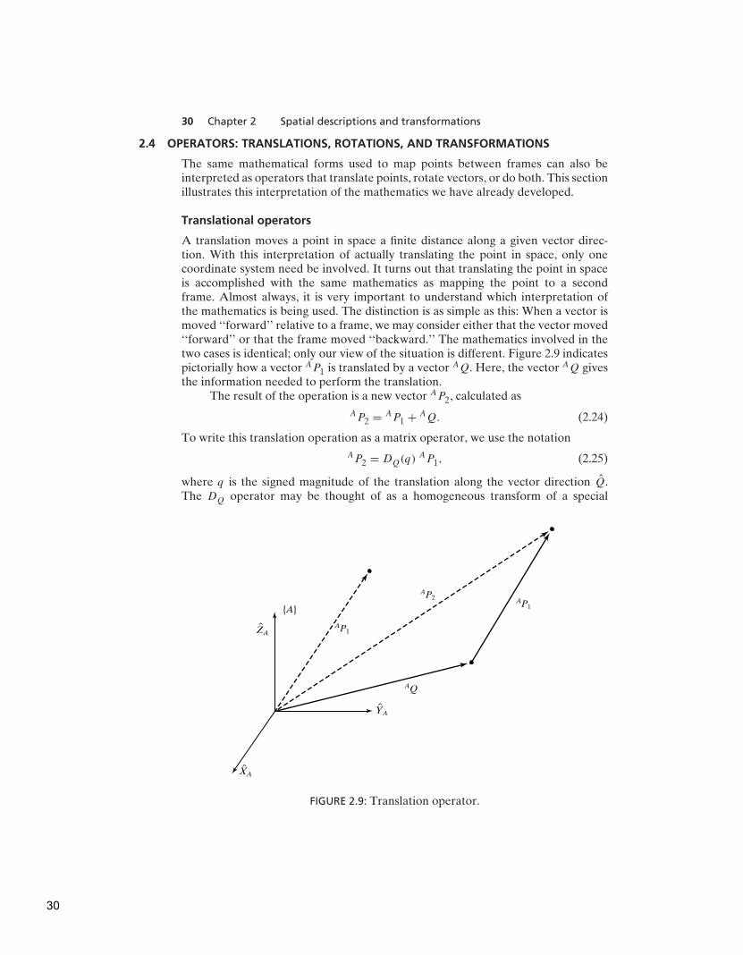
A translation moves a point in space a finite distance along a given vector direc-tion. With this interpretation of actually translating the point in space, only onecoordinate system need be involved. It turns out that translating the point in spaceis accomplished with the same mathematics as mapping the point to a secondframe. Almost always, it is very important to understand which interpretation ofthe mathematics is being used. The distinction is as simple as this: When a vector ismoved ‘‘forward’’ relative to a frame, we may consider either that the vector moved‘‘forward’’ or that the frame moved ‘‘backward.’’ The mathematics involved in thetwo cases is identical; only our view of the situation is different. Figure 2.9 indicatespictorially how a vector AP1 is translated by a vector AQ. Here, the vector AQ givesthe information needed to perform the translation.
The result of the operation is a new vector AP2, calculated as
AP2 = AP1 + AQ. (2.24)
To write this translation operation as a matrix operator, we use the notation
AP2 = DQ(q)AP1, (2.25)
where q is the signed magnitude of the translation along the vector direction Q.The DQ operator may be thought of as a homogeneous transform of a special
AP1
AQ
AP2AP1
ZA
YA
XA
{A}
FIGURE 2.9: Translation operator.
30

Section 2.4 Operators: translations, rotations, and transformations 31
simple form:
DQ(q) =
1 0 0 qx0 1 0 qy0 0 1 qz0 0 0 1
, (2.26)
where qx , qy , and qz are the components of the translation vector Q and q =√
q2x
+ q2y
+ q2z. Equations (2.9) and (2.24) implement the same mathematics. Note
that, if we had defined BPAORG (instead of APBORG) in Fig. 2.4 and had used it in(2.9), then we would have seen a sign change between (2.9) and (2.24). This signchange would indicate the difference between moving the vector ‘‘forward’’ andmoving the coordinate system ‘‘backward.’’ By defining the location of {B} relativeto {A} (with APBORG), we cause the mathematics of the two interpretations to bethe same. Now that the ‘‘DQ’’ notation has been introduced, we may also use it todescribe frames and as a mapping.
Rotational operators
Another interpretation of a rotation matrix is as a rotational operator that operateson a vector AP1 and changes that vector to a new vector, AP2, by means of a rotation,R. Usually, when a rotation matrix is shown as an operator, no sub- or superscriptsappear, because it is not viewed as relating two frames. That is, we may write
AP2 = R AP1. (2.27)
Again, as in the case of translations, the mathematics described in (2.13) and in(2.27) is the same; only our interpretation is different. This fact also allows us to seehow to obtain rotational matrices that are to be used as operators:
The rotation matrix that rotates vectors through some rotation, R, is the same as
the rotation matrix that describes a frame rotated by R relative to the reference frame.Although a rotation matrix is easily viewed as an operator, we will also define
another notation for a rotational operator that clearly indicates which axis is beingrotated about:
AP2 = RK (θ)AP1. (2.28)
In this notation, ‘‘RK (θ)’’ is a rotational operator that performs a rotation about
the axis direction K by θ degrees. This operator can be written as a homogeneoustransform whose position-vector part is zero. For example, substitution into (2.11)yields the operator that rotates about the Z axis by θ as
Rz(�) =
cos θ − sin θ 0 0sin θ cos θ 0 0
0 0 1 00 0 0 1
. (2.29)
Of course, to rotate a position vector, we could just as well use the 3 × 3 rotation-matrix part of the homogeneous transform. The ‘‘RK ’’ notation, therefore, may beconsidered to represent a 3 × 3 or a 4 × 4 matrix. Later in this chapter, we will seehow to write the rotation matrix for a rotation about a general axis K .
31

32 Chapter 2 Spatial descriptions and transformations
XA
YA
{A}
AP1
AP2
FIGURE 2.10: The vector AP1 rotated 30 degrees about Z.
EXAMPLE 2.3
Figure 2.10 shows a vector AP1. We wish to compute the vector obtained by rotating
this vector about Z by 30 degrees. Call the new vector AP2.
The rotation matrix that rotates vectors by 30 degrees about Z is the same asthe rotation matrix that describes a frame rotated 30 degrees about Z relative to thereference frame. Thus, the correct rotational operator is
Rz(30.0) =
0.866 −0.500 0.0000.500 0.866 0.0000.000 0.000 1.000
. (2.30)
Given
AP1 =
0.02.00.0
, (2.31)
we calculate AP2 as
AP2 = Rz(30.0) AP1 =
−1.0001.7320.000
. (2.32)
Equations (2.13) and (2.27) implement the same mathematics. Note that, if wehad defined B
AR (instead of A
BR) in (2.13), then the inverse ofR would appear in (2.27).
This change would indicate the difference between rotating the vector ‘‘forward’’versus rotating the coordinate system ‘‘backward.’’ By defining the location of {B}relative to {A} (by A
BR), we cause the mathematics of the two interpretations to be
the same.
32
Section 2.4 Operators: translations, rotations, and transformations 33
Transformation operators
As with vectors and rotation matrices, a frame has another interpretation asa transformation operator. In this interpretation, only one coordinate system isinvolved, and so the symbol T is used without sub- or superscripts. The operator Trotates and translates a vector AP1 to compute a new vector,
AP2 = T AP1. (2.33)
Again, as in the case of rotations, the mathematics described in (2.18) and in (2.33)is the same, only our interpretation is different. This fact also allows us to see howto obtain homogeneous transforms that are to be used as operators:
The transform that rotates by R and translates by Q is the same as the transform
that describes a frame rotated by R and translated by Q relative to the reference frame.A transform is usually thought of as being in the form of a homogeneous
transform with general rotation-matrix and position-vector parts.
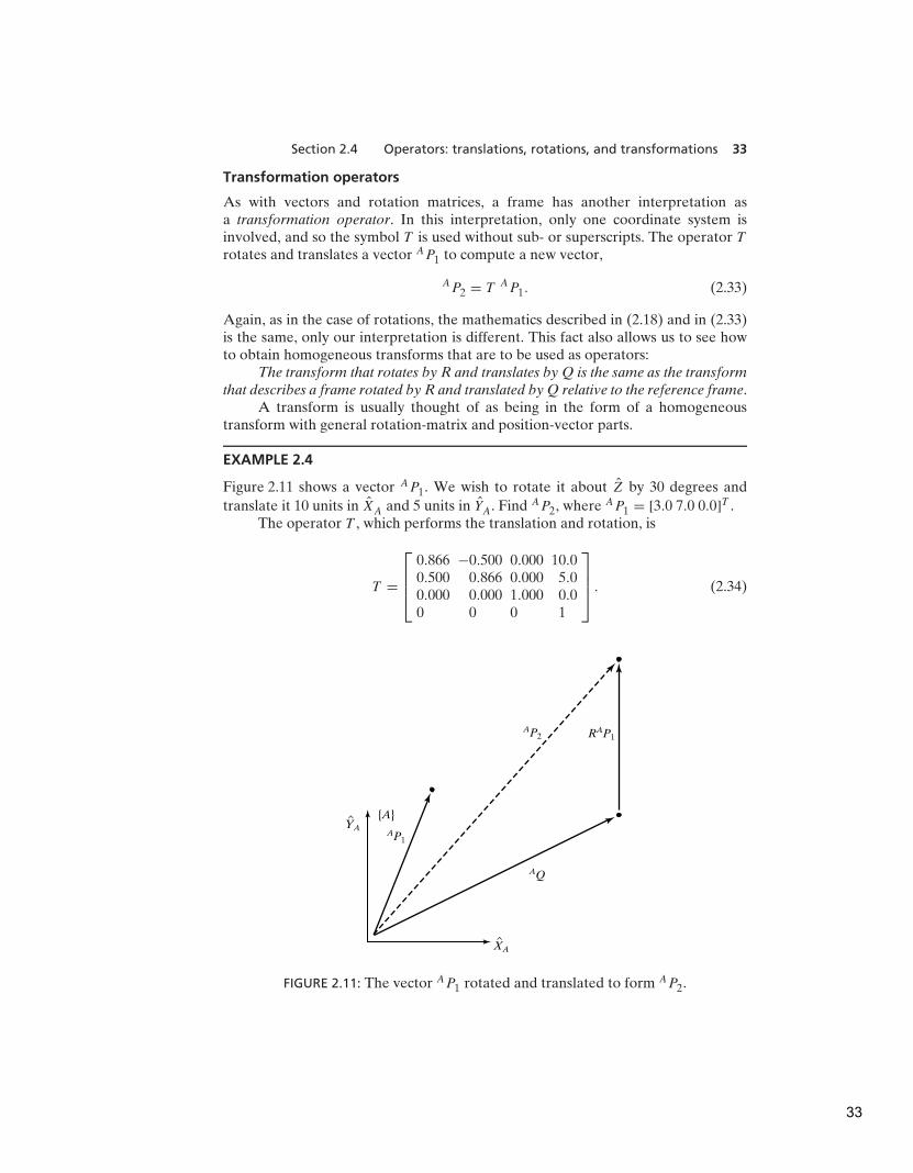
EXAMPLE 2.4
Figure 2.11 shows a vector AP1. We wish to rotate it about Z by 30 degrees and
translate it 10 units in XA and 5 units in YA. Find AP2, where AP1 = [3.0 7.0 0.0]T .The operator T , which performs the translation and rotation, is
T =
0.866 −0.500 0.000 10.00.500 0.866 0.000 5.00.000 0.000 1.000 0.00 0 0 1
. (2.34)
AP1
RAP1AP2
AQ
XA
YA
{A}
FIGURE 2.11: The vector AP1 rotated and translated to form AP2.
33
34 Chapter 2 Spatial descriptions and transformations
Given
AP1 =
3.07.00.0
, (2.35)
we use T as an operator:
AP2 = T AP1 =
9.09812.5620.000
. (2.36)
Note that this example is numerically exactly the same as Example 2.2, but theinterpretation is quite different.
2.5 SUMMARY OF INTERPRETATIONS
We have introduced concepts first for the case of translation only, then for thecase of rotation only, and finally for the general case of rotation about a pointand translation of that point. Having understood the general case of rotation andtranslation, we will not need to explicitly consider the two simpler cases since theyare contained within the general framework.
As a general tool to represent frames, we have introduced the homogeneous
transform, a 4 × 4 matrix containing orientation and position information.We have introduced three interpretations of this homogeneous transform:
1. It is a description of a frame. ABT describes the frame {B} relative to the frame
{A}. Specifically, the columns of ABR are unit vectors defining the directions of
the principal axes of {B}, and APBORG locates the position of the origin of {B}.2. It is a transform mapping. A
BT maps BP → AP .
3. It is a transform operator. T operates on AP1 to create AP2.
From this point on, the terms frame and transform will both be used to referto a position vector plus an orientation. Frame is the term favored in speaking of adescription, and transform is used most frequently when function as a mapping oroperator is implied. Note that transformations are generalizations of (and subsume)translations and rotations; we will often use the term transform when speaking of apure rotation (or translation).
2.6 TRANSFORMATION ARITHMETIC
In this section, we look at the multiplication of transforms and the inversion oftransforms. These two elementary operations form a functionally complete set oftransform operators.
Compound transformations
In Fig. 2.12, we have CP and wish to find AP .
34

Section 2.6 Transformation arithmetic 35
AP
YA
ZA
XA
{A}
CP
YB
ZB
ZC
XB
XC
YC
{B}{C}
FIGURE 2.12: Compound frames: Each is known relative to the previous one.
Frame {C} is known relative to frame {B}, and frame {B} is known relative toframe {A}. We can transform CP into BP as
BP = B
CT CP ; (2.37)
then we can transform BP into AP as
AP = A
BT BP. (2.38)
Combining (2.37) and (2.38), we get the (not unexpected) result
AP = A
BT B
CT CP, (2.39)
from which we could defineA
CT = A
BT B
CT . (2.40)
Again, note that familiarity with the sub- and superscript notation makes thesemanipulations simple. In terms of the known descriptions of {B} and {C}, we cangive the expression for A
CT as
A
CT =
[
ABR B
CR A
BR BPCORG + APBORG
0 0 0 1
]
(2.41)
Inverting a transform
Consider a frame {B} that is known with respect to a frame {A}—that is, we knowthe value of A
BT . Sometimes we will wish to invert this transform, in order to get a
description of {A} relative to {B}—that is, BAT . A straightforward way of calculating
the inverse is to compute the inverse of the 4×4 homogeneous transform. However,if we do so, we are not taking full advantage of the structure inherent in thetransform. It is easy to find a computationally simpler method of computing theinverse, one that does take advantage of this structure.
35
36 Chapter 2 Spatial descriptions and transformations
To find BAT , we must compute B
AR and BPAORG from A
BR and APBORG. First,
recall from our discussion of rotation matrices that
B
AR = A
BRT . (2.42)
Next, we change the description of APBORG into {B} by using (2.13):
B(APBORG) = B
AR APBORG + BPAORG. (2.43)
The left-hand side of (2.43) must be zero, so we have
BPAORG = −B
AR APBORG = −A
BRT APBORG. (2.44)
Using (2.42) and (2.44), we can write the form of BAT as
B
AT =
[
ABRT −A
BRT APBORG
0 0 0 1
]
. (2.45)
Note that, with our notation,B
AT = A
BT −1.
Equation (2.45) is a general and extremely useful way of computing the inverse of ahomogeneous transform.
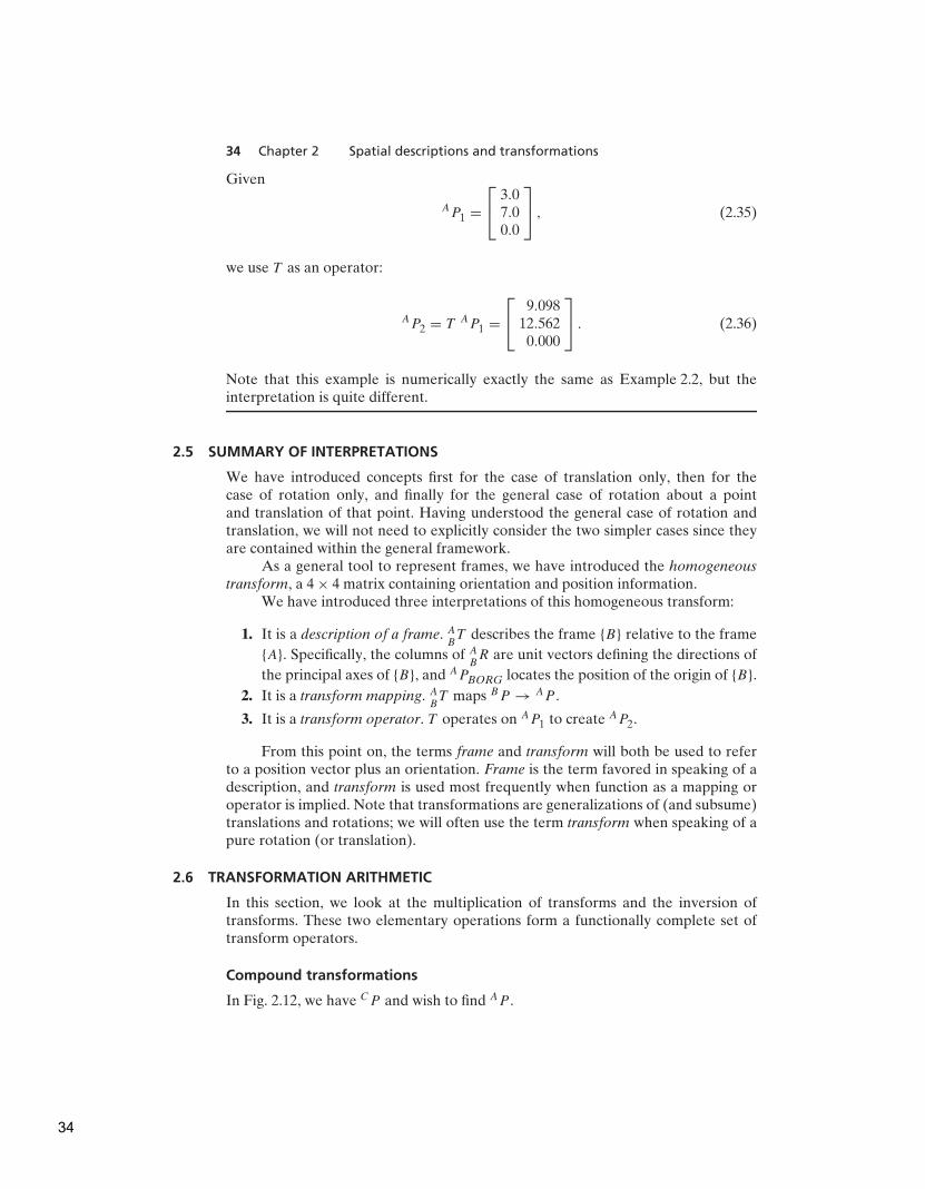
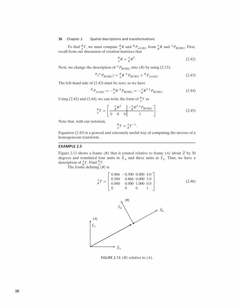
EXAMPLE 2.5
Figure 2.13 shows a frame {B} that is rotated relative to frame {A} about Z by 30degrees and translated four units in XA and three units in YA. Thus, we have adescription of A
BT . Find B
AT .
The frame defining {B} is
A
BT =
0.866 −0.500 0.000 4.00.500 0.866 0.000 3.00.000 0.000 1.000 0.00 0 0 1
. (2.46)
XA
XB
YA
YB
{A}
{B}
FIGURE 2.13: {B} relative to {A}.
36

Section 2.7 Transform equations 37
Using (2.45), we compute
B
AT =
0.866 0.500 0.000 −4.964−0.500 0.866 0.000 −0.598
0.000 0.000 1.000 0.00 0 0 1
. (2.47)
2.7 TRANSFORM EQUATIONS
Figure 2.14 indicates a situation in which a frame {D} can be expressed as productsof transformations in two different ways. First,
U
DT = U
AT A
DT ; (2.48)
second;U
DT = U
BT B
CT C
DT . (2.49)
We can set these two descriptions of UDT equal to construct a transform
equation:U
AT A
DT = U
BT B
CT C
DT . (2.50)
{U}
{A}
{D}
{C}
{B}
FIGURE 2.14: Set of transforms forming a loop.
37
38 Chapter 2 Spatial descriptions and transformations
Transform equations can be used to solve for transforms in the case of n unknowntransforms and n transform equations. Consider (2.50) in the case that all transformsare known except B
CT . Here, we have one transform equation and one unknown
transform; hence, we easily find its solution to be
B
CT = U
BT −1 U
AT A
DT C
DT −1. (2.51)
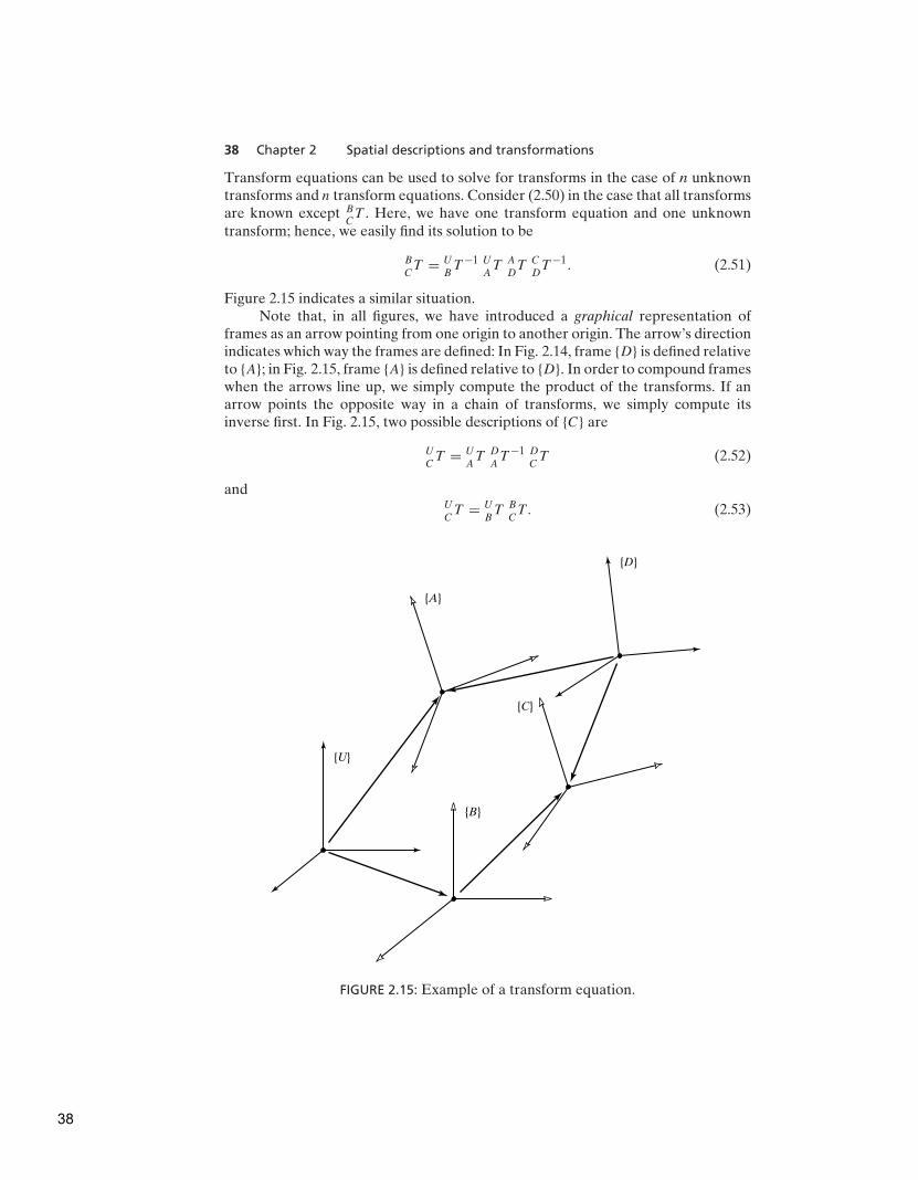
Figure 2.15 indicates a similar situation.Note that, in all figures, we have introduced a graphical representation of
frames as an arrow pointing from one origin to another origin. The arrow’s directionindicates which way the frames are defined: In Fig. 2.14, frame {D} is defined relativeto {A}; in Fig. 2.15, frame {A} is defined relative to {D}. In order to compound frameswhen the arrows line up, we simply compute the product of the transforms. If anarrow points the opposite way in a chain of transforms, we simply compute itsinverse first. In Fig. 2.15, two possible descriptions of {C} are
U
CT = U
AT D
AT −1 D
CT (2.52)
andU
CT = U
BT B
CT . (2.53)
{U}
{A}
{D}
{C}
{B}
FIGURE 2.15: Example of a transform equation.
38
Section 2.8 More on representation of orientation 39
{T }
{G }
{S }
{B }
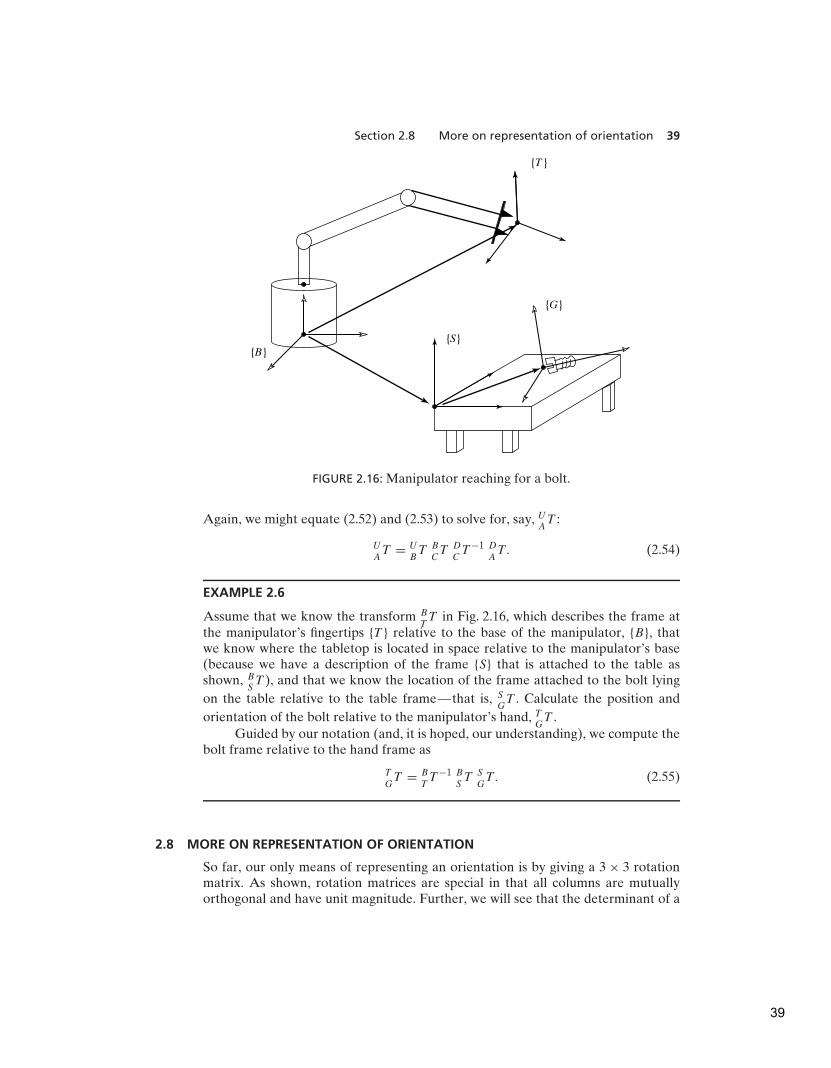
FIGURE 2.16: Manipulator reaching for a bolt.
Again, we might equate (2.52) and (2.53) to solve for, say, UAT :
U
AT = U
BT B
CT D
CT −1 D
AT . (2.54)
EXAMPLE 2.6
Assume that we know the transform BTT in Fig. 2.16, which describes the frame at
the manipulator’s fingertips {T } relative to the base of the manipulator, {B}, thatwe know where the tabletop is located in space relative to the manipulator’s base(because we have a description of the frame {S} that is attached to the table asshown, B
ST ), and that we know the location of the frame attached to the bolt lying
on the table relative to the table frame—that is, SGT . Calculate the position and
orientation of the bolt relative to the manipulator’s hand, TGT .
Guided by our notation (and, it is hoped, our understanding), we compute thebolt frame relative to the hand frame as
T
GT = B
TT −1 B
ST S
GT . (2.55)
2.8 MORE ON REPRESENTATION OF ORIENTATION
So far, our only means of representing an orientation is by giving a 3 × 3 rotationmatrix. As shown, rotation matrices are special in that all columns are mutuallyorthogonal and have unit magnitude. Further, we will see that the determinant of a
39

40 Chapter 2 Spatial descriptions and transformations
rotation matrix is always equal to +1. Rotation matrices may also be called properorthonormal matrices, where ‘‘proper’’ refers to the fact that the determinant is +1(nonproper orthonormal matrices have the determinant −1).
It is natural to ask whether it is possible to describe an orientation with fewerthan nine numbers. A result from linear algebra (known as Cayley’s formula fororthonormal matrices [3]) states that, for any proper orthonormal matrix R, thereexists a skew-symmetric matrix S such that
R = (I3 − S)−1(I3 + S), (2.56)
where I3 is a 3 × 3 unit matrix. Now a skew-symmetric matrix (i.e., S = −ST ) ofdimension 3 is specified by three parameters (sx, sy, sz) as
S =
0 −sx sysx 0 −sx
−sy sx 0
. (2.57)
Therefore, an immediate consequence of formula (2.56) is that any 3 × 3 rotationmatrix can be specified by just three parameters.
Clearly, the nine elements of a rotation matrix are not all independent. In fact,given a rotation matrix, R, it is easy to write down the six dependencies between theelements. Imagine R as three columns, as originally introduced:
R = [X Y Z]. (2.58)
As we know from Section 2.2, these three vectors are the unit axes of some framewritten in terms of the reference frame. Each is a unit vector, and all three must bemutually perpendicular, so we see that there are six constraints on the nine matrixelements:
|X| = 1,
|Y | = 1,
|Z| = 1, (2.59)
X · Y = 0,
X · Z = 0,
Y · Z = 0.
It is natural then to ask whether representations of orientation can be devised suchthat the representation is conveniently specified with three parameters. This sectionwill present several such representations.
Whereas translations along three mutually perpendicular axes are quite easyto visualize, rotations seem less intuitive. Unfortunately, people have a hard timedescribing and specifying orientations in three-dimensional space. One difficulty isthat rotations don’t generally commute. That is, A
BR B
CR is not the same as B
CR A
BR.
40

Section 2.8 More on representation of orientation 41
EXAMPLE 2.7
Consider two rotations, one about Z by 30 degrees and one about X by 30 degrees:
Rz(30) =
0.866 −0.500 0.0000.500 0.866 0.0000.000 0.000 1.000
(2.60)
Rx(30) =
1.000 0.000 0.0000.000 0.866 −0.5000.000 0.500 0.866
(2.61)
Rz(30)Rx(30) =
0.87 −0.43 0.250.50 0.75 −0.430.00 0.50 0.87
�= Rx(30)Rz(30) =
0.87 −0.50 0.000.43 0.75 −0.500.25 0.43 0.87
(2.62)
The fact that the order of rotations is important should not be surprising; further-more, it is captured in the fact that we use matrices to represent rotations, becausemultiplication of matrices is not commutative in general.
Because rotations can be thought of either as operators or as descriptions oforientation, it is not surprising that different representations are favored for eachof these uses. Rotation matrices are useful as operators. Their matrix form is suchthat, when multiplied by a vector, they perform the rotation operation. However,rotation matrices are somewhat unwieldy when used to specify an orientation. Ahuman operator at a computer terminal who wishes to type in the specificationof the desired orientation of a robot’s hand would have a hard time inputting anine-element matrix with orthonormal columns. A representation that requires onlythree numbers would be simpler. The following sections introduce several suchrepresentations.
X–Y–Z fixed angles
One method of describing the orientation of a frame {B} is as follows:
Start with the frame coincident with a known reference frame {A}.Rotate {B} first about XA by an angle γ , then about YA by an angle β,
and, finally, about ZA by an angle α.
Each of the three rotations takes place about an axis in the fixed referenceframe {A}. We will call this convention for specifying an orientation X–Y–Z fixedangles. The word ‘‘fixed’’ refers to the fact that the rotations are specified aboutthe fixed (i.e., nonmoving) reference frame (Fig. 2.17). Sometimes this conventionis referred to as roll, pitch, yaw angles, but care must be used, as this name is oftengiven to other related but different conventions.
41

42 Chapter 2 Spatial descriptions and transformations
ZB�
ZB�
YB�
ZB�
XB�
YB�
XB�
YB�
XB�
XA
YA YA YA
XA
ZA
XA
ZA
ZA
g
b
a
FIGURE 2.17: X–Y–Z fixed angles. Rotations are performed in the order RX(γ ),RY (β), RZ(α).
The derivation of the equivalent rotation matrix, ABRXYZ(γ, β, α), is straight-
forward, because all rotations occur about axes of the reference frame; that is,
A
BRXYZ(γ, β, α) = RZ(α)RY (β)RX(γ )
=
cα −sα 0sα cα 00 0 1
cβ 0 sβ
0 1 0−sβ 0 cβ
1 0 00 cγ −sγ
0 sγ cγ
, (2.63)
where cα is shorthand for cos α, sα for sin α, and so on. It is extremely important tounderstand the order of rotations used in (2.63). Thinking in terms of rotations asoperators, we have applied the rotations (from the right) of RX(γ ), then RY (β), andthen RZ(α). Multiplying (2.63) out, we obtain
A
BRXYZ(γ, β, α) =
cαcβ cαsβsγ − sαcγ cαsβcγ + sαsγ
sαcβ sαsβsγ + cαcγ sαsβcγ − cαsγ
−sβ cβsγ cβcγ
. (2.64)
Keep in mind that the definition given here specifies the order of the three rotations.Equation (2.64) is correct only for rotations performed in the order: about XA by γ ,
about YA by β, about ZA by α.The inverse problem, that of extracting equivalent X–Y–Z fixed angles from
a rotation matrix, is often of interest. The solution depends on solving a set oftranscendental equations: there are nine equations and three unknowns if (2.64) isequated to a given rotation matrix. Among the nine equations are six dependencies,so, essentially, we have three equations and three unknowns. Let
A
BRXYZ(γ, β, α) =
r11 r12 r13r21 r22 r23r31 r32 r33
. (2.65)
From (2.64), we see that, by taking the square root of the sum of the squaresof r11 and r21, we can compute cos β. Then, we can solve for β with the arc tangent
42
Section 2.8 More on representation of orientation 43
of −r31 over the computed cosine. Then, as long as cβ �= 0, we can solve for α bytaking the arc tangent of r21/cβ over r11/cβ and we can solve for γ by taking the arctangent of r32/cβ over r33/cβ.
In summary,
β = Atan2(−r31,
√
r211
+ r221),
α = Atan2(r21/cβ, r11/cβ), (2.66)
γ = Atan2(r32/cβ, r33/cβ),
where Atan2(y, x) is a two-argument arc tangent function.3
Although a second solution exists, by using the positive square root in theformula for β, we always compute the single solution for which −90.0◦ ≤ β ≤ 90.0◦.This is usually a good practice, because we can then define one-to-one mappingfunctions between various representations of orientation. However, in some cases,calculating all solutions is important (more on this in Chapter 4). If β = ±90.0◦ (sothat cβ = 0), the solution of (2.67) degenerates. In those cases, only the sum orthe difference of α and γ can be computed. One possible convention is to chooseα = 0.0 in these cases, which has the results given next.
If β = 90.0◦, then a solution can be calculated to be
β = 90.0◦,
α = 0.0, (2.67)
γ = Atan2(r12, r22).
If β = −90.0◦, then a solution can be calculated to be
β = −90.0◦,
α = 0.0, (2.68)
γ = −Atan2(r12, r22).
Z–Y–X Euler angles
Another possible description of a frame {B} is as follows:
Start with the frame coincident with a known frame {A}. Rotate {B} firstabout ZB by an angle α, then about YB by an angle β, and, finally, about
XB by an angle γ .
In this representation, each rotation is performed about an axis of the movingsystem {B} rather than one of the fixed reference {A}. Such sets of three rotations
3Atan2(y, x) computes tan−1(yx ) but uses the signs of both x and y to identify the quadrant in which
the resulting angle lies. For example, Atan 2(−2.0,−2.0) = −135◦, whereas Atan 2(2.0, 2.0) = 45◦, adistinction which would be lost with a single-argument arc tangent function. We are frequently computingangles that can range over a full 360◦, so we will make use of the Atan2 function regularly. Note thatAtan2 becomes undefined when both arguments are zero. It is sometimes called a ‘‘4-quadrant arctangent,’’ and some programming-language libraries have it predefined.
43
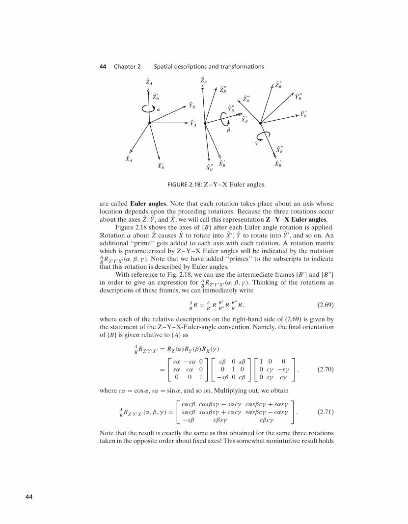
44 Chapter 2 Spatial descriptions and transformations
ZB�
XB�
XB�
XB�
YB�
ZB�
ZB� YB
�
XB�
YB�
ZB�
YB�
XB�
ZAZB
YB
YA
XA
a
b
g
FIGURE 2.18: Z–Y–X Euler angles.
are called Euler angles. Note that each rotation takes place about an axis whoselocation depends upon the preceding rotations. Because the three rotations occurabout the axes Z, Y , and X, we will call this representation Z–Y–X Euler angles.
Figure 2.18 shows the axes of {B} after each Euler-angle rotation is applied.Rotation α about Z causes X to rotate into X′, Y to rotate into Y ′, and so on. Anadditional ‘‘prime’’ gets added to each axis with each rotation. A rotation matrixwhich is parameterized by Z–Y–X Euler angles will be indicated by the notationABRZ′Y ′X′(α, β, γ ). Note that we have added ‘‘primes’’ to the subscripts to indicate
that this rotation is described by Euler angles.With reference to Fig. 2.18, we can use the intermediate frames {B ′} and {B ′′}
in order to give an expression for ABRZ′Y ′X′(α, β, γ ). Thinking of the rotations as
descriptions of these frames, we can immediately write
A
BR = A
B ′RB ′
B ′′RB ′′
BR, (2.69)
where each of the relative descriptions on the right-hand side of (2.69) is given bythe statement of the Z–Y–X-Euler-angle convention. Namely, the final orientationof {B} is given relative to {A} as
A
BRZ′Y ′X′ = RZ(α)RY (β)RX(γ )
=
cα −sα 0sα cα 00 0 1
cβ 0 sβ
0 1 0−sβ 0 cβ
1 0 00 cγ −sγ
0 sγ cγ
, (2.70)
where cα = cosα, sα = sinα, and so on. Multiplying out, we obtain
A
BRZ′Y ′X′(α, β, γ ) =
cαcβ cαsβsγ − sαcγ cαsβcγ + sαsγ
sαcβ sαsβsγ + cαcγ sαsβcγ − cαsγ
−sβ cβsγ cβcγ
. (2.71)
Note that the result is exactly the same as that obtained for the same three rotationstaken in the opposite order about fixed axes! This somewhat nonintuitive result holds
44
Section 2.8 More on representation of orientation 45
in general: three rotations taken about fixed axes yield the same final orientationas the same three rotations taken in opposite order about the axes of the movingframe.
Because (2.71) is equivalent to (2.64), there is no need to repeat the solutionfor extracting Z–Y–X Euler angles from a rotation matrix. That is, (2.66) can alsobe used to solve for Z–Y–X Euler angles that correspond to a given rotation matrix.
Z–Y–Z Euler angles
Another possible description of a frame {B} is
Start with the frame coincident with a known frame {A}. Rotate {B} firstabout ZB by an angle α, then about YB by an angle β, and, finally, aboutZb by an angle γ .
Rotations are described relative to the frame we are moving, namely, {B}, sothis is an Euler-angle description. Because the three rotations occur about the axesZ, Y , and Z, we will call this representation Z–Y–Z Euler angles.
Following the development exactly as in the last section, we arrive at theequivalent rotation matrix
A
BRZ′Y ′Z′(α, β, γ ) =
cαcβcγ − sαsγ −cαcβsγ − sαcγ cαsβ
sαcβcγ + cαsγ −sαcβsγ + cαcγ sαsβ
−sβcγ sβsγ cβ
. (2.72)
The solution for extracting Z–Y–Z Euler angles from a rotation matrix isstated next.
Given
A
BRZ′Y ′Z′(α, β, γ ) =
r11 r12 r13r21 r22 r23r31 r32 r33
, (2.73)
then, if sin β �= 0, it follows that
β = Atan2(√
r231
+ r232, r33),
α = Atan2(r23/sβ, r13/sβ), (2.74)
γ = Atan2(r32/sβ,−r31/sβ).
Although a second solution exists (which we find by using the positive square root inthe formula for β), we always compute the single solution for which 0.0 ≤ β ≤ 180.0◦.If β = 0.0 or 180.0◦, the solution of (2.74) degenerates. In those cases, only the sumor the difference of α and γ may be computed. One possible convention is to chooseα = 0.0 in these cases, which has the results given next.
If β = 0.0, then a solution can be calculated to be
β = 0.0,
α = 0.0, (2.75)
γ = Atan2(−r12, r11).
45
46 Chapter 2 Spatial descriptions and transformations
If β = 180.0◦, then a solution can be calculated to be
β = 180.0◦,
α = 0.0, (2.76)
γ = Atan2(r12,−r11).
Other angle-set conventions
In the preceding subsections we have seen three conventions for specifying orienta-tion: X–Y–Z fixed angles, Z–Y–X Euler angles, and Z–Y–Z Euler angles. Eachof these conventions requires performing three rotations about principal axes in acertain order. These conventions are examples of a set of 24 conventions that wewill call angle-set conventions. Of these, 12 conventions are for fixed-angle sets,and 12 are for Euler-angle sets. Note that, because of the duality of fixed-anglesets with Euler-angle sets, there are really only 12 unique parameterizations of arotation matrix by using successive rotations about principal axes. There is oftenno particular reason to favor one convention over another, but various authorsadopt different ones, so it is useful to list the equivalent rotation matrices for all 24conventions. Appendix B (in the back of the book) gives the equivalent rotationmatrices for all 24 conventions.
Equivalent angle–axis representation
With the notation RX(30.0) we give the description of an orientation by giving an
axis, X, and an angle, 30.0 degrees. This is an example of an equivalent angle–axisrepresentation. If the axis is a general direction (rather than one of the unit directions)any orientation may be obtained through proper axis and angle selection. Considerthe following description of a frame {B}:
Start with the frame coincident with a known frame {A}; then rotate {B}about the vector AK by an angle θ according to the right-hand rule.
Vector K is sometimes called the equivalent axis of a finite rotation. A generalorientation of {B} relative to {A} may be written as A
BR(K, θ) or RK (θ) and will
be called the equivalent angle–axis representation.4 The specification of the vectorAK requires only two parameters, because its length is always taken to be one. Theangle specifies a third parameter. Often, we will multiply the unit direction, K , withthe amount of rotation, θ , to form a compact 3 × 1 vector description of orientation,denoted by K (no ‘‘hat’’). See Fig. 2.19.
When the axis of rotation is chosen from among the principal axes of {A}, thenthe equivalent rotation matrix takes on the familiar form of planar rotations:
RX(θ) =
1 1 00 cos θ − sin θ0 sin θ cos θ
, (2.77)
4That such a K and θ exist for any orientation of {B} relative to {A} was shown originally by Eulerand is known as Euler’s theorem on rotation [3].
46
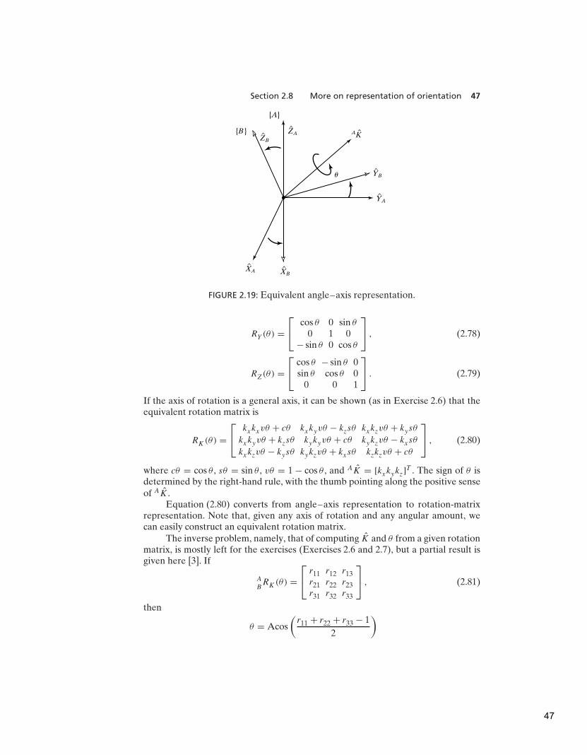
Section 2.8 More on representation of orientation 47
ZB
ZA
XA XB
YA
YB
AK
{A}
{B }
u
FIGURE 2.19: Equivalent angle–axis representation.
RY (θ) =
cos θ 0 sin θ0 1 0
− sin θ 0 cos θ
, (2.78)
RZ(θ) =
cos θ − sin θ 0sin θ cos θ 0
0 0 1
. (2.79)
If the axis of rotation is a general axis, it can be shown (as in Exercise 2.6) that theequivalent rotation matrix is
RK(θ) =
kxkxvθ + cθ kxkyvθ − kzsθ kxkzvθ + kysθ
kxkyvθ + kzsθ kykyvθ + cθ kykzvθ − kxsθ
kxkzvθ − kysθ kykzvθ + kxsθ kzkzvθ + cθ
, (2.80)
where cθ = cos θ , sθ = sin θ , vθ = 1 − cos θ , and AK = [kxkykz]T . The sign of θ isdetermined by the right-hand rule, with the thumb pointing along the positive senseof AK .
Equation (2.80) converts from angle–axis representation to rotation-matrixrepresentation. Note that, given any axis of rotation and any angular amount, wecan easily construct an equivalent rotation matrix.
The inverse problem, namely, that of computing K and θ from a given rotationmatrix, is mostly left for the exercises (Exercises 2.6 and 2.7), but a partial result isgiven here [3]. If
A
BRK (θ) =
r11 r12 r13r21 r22 r23r31 r32 r33
, (2.81)
then
θ = Acos
(
r11 + r22 + r33 − 1
2
)
47
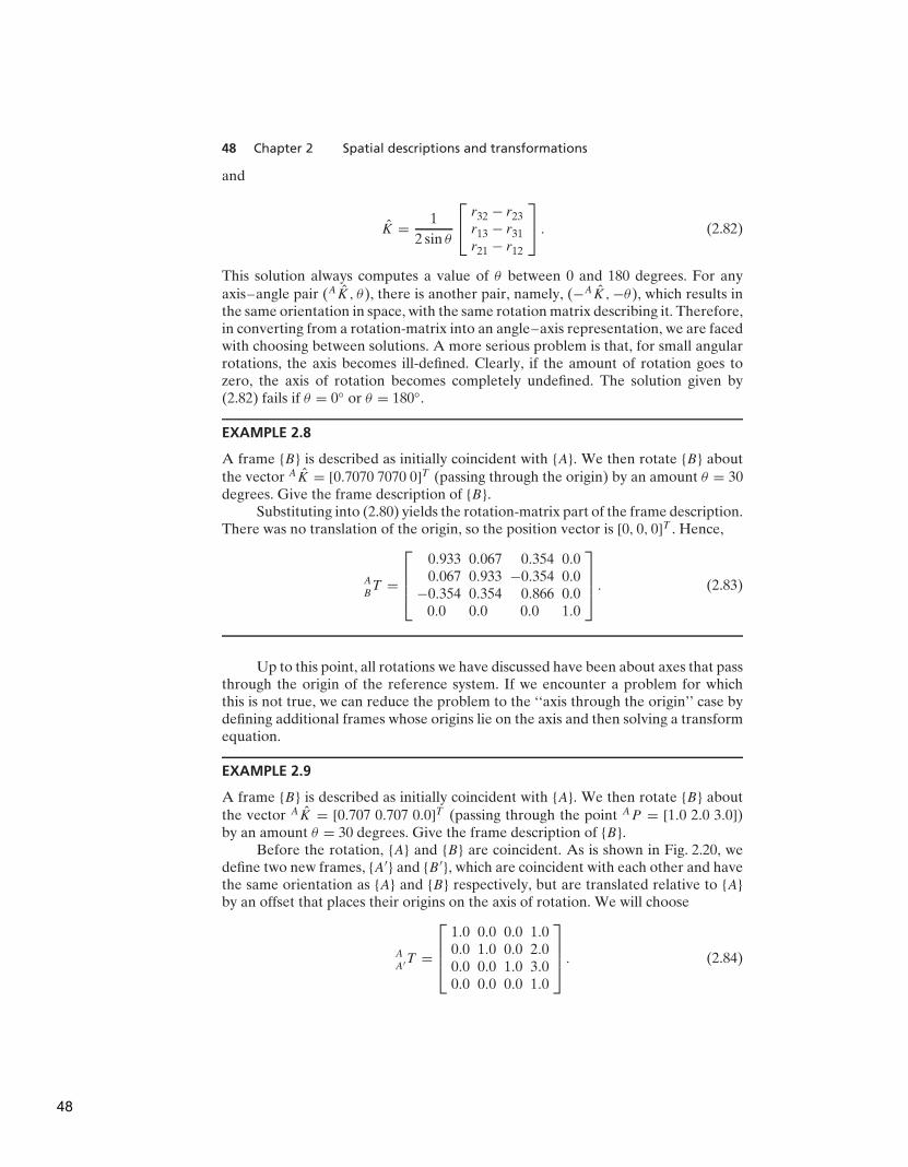
48 Chapter 2 Spatial descriptions and transformations
and
K = 1
2 sin θ
r32 − r23r13 − r31r21 − r12
. (2.82)
This solution always computes a value of θ between 0 and 180 degrees. For anyaxis–angle pair (AK, θ), there is another pair, namely, (−AK,−θ), which results inthe same orientation in space, with the same rotation matrix describing it. Therefore,in converting from a rotation-matrix into an angle–axis representation, we are facedwith choosing between solutions. A more serious problem is that, for small angularrotations, the axis becomes ill-defined. Clearly, if the amount of rotation goes tozero, the axis of rotation becomes completely undefined. The solution given by(2.82) fails if θ = 0◦ or θ = 180◦.
EXAMPLE 2.8
A frame {B} is described as initially coincident with {A}. We then rotate {B} aboutthe vector AK = [0.7070 7070 0]T (passing through the origin) by an amount θ = 30degrees. Give the frame description of {B}.
Substituting into (2.80) yields the rotation-matrix part of the frame description.There was no translation of the origin, so the position vector is [0, 0, 0]T . Hence,
A
BT =
0.933 0.067 0.354 0.00.067 0.933 −0.354 0.0
−0.354 0.354 0.866 0.00.0 0.0 0.0 1.0
. (2.83)
Up to this point, all rotations we have discussed have been about axes that passthrough the origin of the reference system. If we encounter a problem for whichthis is not true, we can reduce the problem to the ‘‘axis through the origin’’ case bydefining additional frames whose origins lie on the axis and then solving a transformequation.
EXAMPLE 2.9
A frame {B} is described as initially coincident with {A}. We then rotate {B} aboutthe vector AK = [0.707 0.707 0.0]T (passing through the point AP = [1.0 2.0 3.0])by an amount θ = 30 degrees. Give the frame description of {B}.
Before the rotation, {A} and {B} are coincident. As is shown in Fig. 2.20, wedefine two new frames, {A′} and {B ′}, which are coincident with each other and havethe same orientation as {A} and {B} respectively, but are translated relative to {A}by an offset that places their origins on the axis of rotation. We will choose
A
A′T =
1.0 0.0 0.0 1.00.0 1.0 0.0 2.00.0 0.0 1.0 3.00.0 0.0 0.0 1.0
. (2.84)
48

Section 2.8 More on representation of orientation 49
{A}
{B }
AP
{B�} {A�}K
FIGURE 2.20: Rotation about an axis that does not pass through the origin of {A}.Initially, {B} was coincident with {A}.
Similarly, the description of {B} in terms of {B ′} is
B ′
BT =
1.0 0.0 0.0 −1.00.0 1.0 0.0 −2.00.0 0.0 1.0 −3.00.0 0.0 0.0 1.0
. (2.85)
Now, keeping other relationships fixed, we can rotate {B ′} relative to {A′}. This is arotation about an axis that passes through the origin, so we can use (2.80) to compute{B ′} relative to {A′}. Substituting into (2.80) yields the rotation-matrix part of theframe description. There was no translation of the origin, so the position vector is[0, 0, 0]T . Thus, we have
A′
B ′T =
0.933 0.067 0.354 0.00.067 0.933 −0.354 0.0
−0.354 0.354 0.866 0.00.0 0.0 0.0 1.0
. (2.86)
Finally, we can write a transform equation to compute the desired frame,
A
BT = A
A′TA′
B ′TB ′
BT , (2.87)
which evaluates to
A
BT =
0.933 0.067 0.354 −1.130.067 0.933 −0.354 1.13
−0.354 0.354 0.866 0.050.000 0.000 0.000 1.00
. (2.88)
A rotation about an axis that does not pass through the origin causes a change inposition, plus the same final orientation as if the axis had passed through the origin.
49
50 Chapter 2 Spatial descriptions and transformations
Note that we could have used any definition of {A′} and {B ′} such that their originswere on the axis of rotation. Our particular choice of orientation was arbitrary, andour choice of the position of the origin was one of an infinity of possible choiceslying along the axis of rotation. (See also Exercise 2.14.)
Euler parameters
Another representation of orientation is by means of four numbers called the Eulerparameters. Although complete discussion is beyond the scope of the book, we statethe convention here for reference.
In terms of the equivalent axis K = [kx ky kz]T and the equivalent angle θ , theEuler parameters are given by
ǫ1 = kx sinθ
2,
ǫ2 = ky sinθ
2, (2.89)
ǫ3 = kz sinθ
2,
ǫ4 = cosθ
2.
It is then clear that these four quantities are not independent:
ǫ21
+ ǫ22
+ ǫ23
+ ǫ24
= 1 (2.90)
must always hold. Hence, an orientation might be visualized as a point on a unithypersphere in four-dimensional space.
Sometimes, the Euler parameters are viewed as a 3 × 1 vector plus a scalar.However, as a 4 × 1 vector, the Euler parameters are known as a unit quaternion.
The rotation matrix Rǫ that is equivalent to a set of Euler parameters is
Rǫ =
1 − 2ǫ22
− 2ǫ23
2(ǫ1ǫ2 − ǫ3ǫ4) 2(ǫ1ǫ3 + ǫ2ǫ4)
2(ǫ1ǫ2 + ǫ3ǫ4) 1 − 2ǫ21
− 2ǫ23
2(ǫ2ǫ3 − ǫ1ǫ4)
2(ǫ1ǫ3 − ǫ2ǫ4) 2(ǫ2ǫ3 + ǫ1ǫ4) 1 − 2ǫ21
− 2ǫ22
. (2.91)
Given a rotation matrix, the equivalent Euler parameters are
ǫ1 = r32 − r23
4ǫ4
,
ǫ2 = r13 − r31
4ǫ4
, (2.92)
ǫ3 = r21 − r12
4ǫ4
,
ǫ4 = 1
2
√
1 + r11 + r22 + r33.
50
Section 2.9 Transformation of free vectors 51
Note that (2.92) is not useful in a computational sense if the rotation matrixrepresents a rotation of 180 degrees about some axis, because ǫ4 goes to zero.However, it can be shown that, in the limit, all the expressions in (2.92) remain finiteeven for this case. In fact, from the definitions in (2.88), it is clear that all ǫi remainin the interval [−1, 1].
Taught and predefined orientations
In many robot systems, it will be possible to ‘‘teach’’ positions and orientationsby using the robot itself. The manipulator is moved to a desired location, and thisposition is recorded. A frame taught in this manner need not necessarily be one towhich the robot will be commanded to return; it could be a part location or a fixturelocation. In other words, the robot is used as a measuring tool having six degreesof freedom. Teaching an orientation like this completely obviates the need for thehuman programmer to deal with orientation representation at all. In the computer,the taught point is stored as a rotation matrix (or however), but the user never hasto see or understand it. Robot systems that allow teaching of frames by using therobot are thus highly recommended.
Besides teaching frames, some systems have a set of predefined orientations,such as ‘‘pointing down’’ or ‘‘pointing left.’’ These specifications are very easyfor humans to deal with. However, if this were the only means of describing andspecifying orientation, the system would be very limited.
2.9 TRANSFORMATION OF FREE VECTORS
We have been concerned mostly with position vectors in this chapter. In laterchapters, we will discuss velocity and force vectors as well. These vectors willtransform differently because they are a different type of vector.
In mechanics, one makes a distinction between the equality and the equivalenceof vectors. Two vectors are equal if they have the same dimensions, magnitude, and
direction. Two vectors that are considered equal could have different lines ofaction—for example, the three equal vectors in Fig 2.21. These velocity vectorshave the same dimensions, magnitude, and direction and so are equal according toour definition.
Two vectors are equivalent in a certain capacity if each produces the very same
effect in this capacity. Thus, if the criterion in Fig. 2.21 is distance traveled, all threevectors give the same result and are thus equivalent in this capacity. If the criterion isheight above the xy plane, then the vectors are not equivalent despite their equality.Thus, relationships between vectors and notions of equivalence depend entirely on
the situation at hand. Furthermore, vectors that are not equal might cause equivalenteffects in certain cases.
We will define two basic classes of vector quantities that might be helpful.The term line vector refers to a vector that is dependent on its line of action,
along with direction and magnitude, for causing its effects. Often, the effects of aforce vector depend upon its line of action (or point of application), so it would thenbe considered a line vector.
A free vector refers to a vector that may be positioned anywhere in space with-out loss or change of meaning, provided that magnitude and direction are preserved.
51
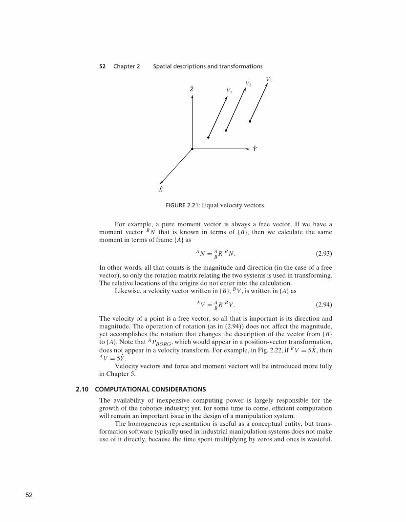
52 Chapter 2 Spatial descriptions and transformations
V1
V2
V3
Z
Y
X
FIGURE 2.21: Equal velocity vectors.
For example, a pure moment vector is always a free vector. If we have amoment vector BN that is known in terms of {B}, then we calculate the samemoment in terms of frame {A} as
AN = A
BR BN. (2.93)
In other words, all that counts is the magnitude and direction (in the case of a freevector), so only the rotation matrix relating the two systems is used in transforming.The relative locations of the origins do not enter into the calculation.
Likewise, a velocity vector written in {B}, BV , is written in {A} as
AV = A
BR BV. (2.94)
The velocity of a point is a free vector, so all that is important is its direction andmagnitude. The operation of rotation (as in (2.94)) does not affect the magnitude,yet accomplishes the rotation that changes the description of the vector from {B}to {A}. Note that APBORG, which would appear in a position-vector transformation,
does not appear in a velocity transform. For example, in Fig. 2.22, if BV = 5X, thenAV = 5Y .
Velocity vectors and force and moment vectors will be introduced more fullyin Chapter 5.
2.10 COMPUTATIONAL CONSIDERATIONS
The availability of inexpensive computing power is largely responsible for thegrowth of the robotics industry; yet, for some time to come, efficient computationwill remain an important issue in the design of a manipulation system.
The homogeneous representation is useful as a conceptual entity, but trans-formation software typically used in industrial manipulation systems does not makeuse of it directly, because the time spent multiplying by zeros and ones is wasteful.
52

Section 2.10 Computational considerations 53
YB
XB
XA
YA
ZB
ZA
{B }
{A}
V
FIGURE 2.22: Transforming velocities.
Usually, the computations shown in (2.41) and (2.45) are performed, rather than thedirect multiplication or inversion of 4 × 4 matrices.
The order in which transformations are applied can make a large differencein the amount of computation required to compute the same quantity. Considerperforming multiple rotations of a vector, as in
AP = A
BR B
CR C
DR DP. (2.95)
One choice is to first multiply the three rotation matrices together, to form ADR in
the expressionAP = A
DR DP. (2.96)
Forming ADR from its three constituents requires 54 multiplications and 36 additions.
Performing the final matrix-vector multiplication of (2.96) requires an additional9 multiplications and 6 additions, bringing the totals to 63 multiplications and 42additions.
If, instead, we transform the vector through the matrices one at a time, that is,
AP = A
BR B
CR C
DR DP
AP = A
BR B
CR CP (2.97)
AP = A
BR BP
AP = AP,
then the total computation requires only 27 multiplications and 18 additions, fewerthan half the computations required by the other method.
Of course, in some cases, the relationships ABR, B
CR, and C
DR are constant, while
there are many DPi that need to be transformed into APi . In such a case, it is moreefficient to calculate A
DR once, and then use it for all future mappings. See also
Exercise 2.16.
53
54 Chapter 2 Spatial descriptions and transformations
EXAMPLE 2.10
Give a method of computing the product of two rotation matrices, ABR B
CR, that uses
fewer than 27 multiplications and 18 additions.Where Li are the columns of B
CR and Ci are the three columns of the result,
compute
C1 = A
BRLi,
C2 = A
BRL2, (2.98)
C3 = C1 × C2,
which requires 24 multiplications and 15 additions.
BIBLIOGRAPHY
[1] B. Noble, Applied Linear Algebra, Prentice-Hall, Englewood Cliffs, NJ, 1969.
[2] D. Ballard and C. Brown, Computer Vision, Prentice-Hall, Englewood Cliffs, NJ, 1982.
[3] O. Bottema and B. Roth, Theoretical Kinematics, North Holland, Amsterdam, 1979.
[4] R.P. Paul, Robot Manipulators, MIT Press, Cambridge, MA, 1981.
[5] I. Shames, Engineering Mechanics, 2nd edition, Prentice-Hall, Englewood Cliffs, NJ,1967.
[6] Symon, Mechanics, 3rd edition, Addison-Wesley, Reading, MA, 1971.
[7] B. Gorla and M. Renaud, Robots Manipulateurs, Cepadues-Editions, Toulouse, 1984.
EXERCISES
2.1 [15] A vector AP is rotated about ZA by θ degrees and is subsequently rotated
about XA by φ degrees. Give the rotation matrix that accomplishes these rotationsin the given order.
2.2 [15] A vector AP is rotated about YA by 30 degrees and is subsequently rotated
about XA by 45 degrees. Give the rotation matrix that accomplishes these rotationsin the given order.
2.3 [16] A frame {B} is located initially coincident with a frame {A}. We rotate {B}about ZB by θ degrees, and then we rotate the resulting frame about XB by φ
degrees. Give the rotation matrix that will change the descriptions of vectors fromBP to AP .
2.4 [16] A frame {B} is located initially coincident with a frame {A}. We rotate {B}about ZB by 30 degrees, and then we rotate the resulting frame about XB by 45degrees. Give the rotation matrix that will change the description of vectors fromBP to AP .
2.5 [13] ABR is a 3 × 3 matrix with eigenvalues 1, e+ai , and e−ai , where i =
√−1. What
is the physical meaning of the eigenvector of ABR associated with the eigenvalue 1?
2.6 [21] Derive equation (2.80).2.7 [24] Describe (or program) an algorithm that extracts the equivalent angle and
axis of a rotation matrix. Equation (2.82) is a good start, but make sure that youralgorithm handles the special cases θ = 0◦ and θ = 180◦.
54

Exercises 55
2.8 [29] Write a subroutine that changes representation of orientation from rotation-matrix form to equivalent angle–axis form. A Pascal-style procedure declarationwould begin
Procedure RMTOAA (VAR R:mat33; VAR K:vec3; VAR theta: real);
Write another subroutine that changes from equivalent angle–axis representationto rotation-matrix representation:
Procedure AATORM(VAR K:vec3; VAR theta: real: VAR R:mat33);
Write the routines in C if you prefer.Run these procedures on several cases of test data back-to-back and verify thatyou get back what you put in. Include some of the difficult cases!
2.9 [27] Do Exercise 2.8 for roll, pitch, yaw angles about fixed axes.2.10 [27] Do Exercise 2.8 for Z–Y–Z Euler angles.2.11 [10] Under what condition do two rotation matrices representing finite rotations
commute? A proof is not required.2.12 [14] A velocity vector is given by
BV =
10.020.030.0
.
Given
A
BT =
0.866 −0.500 0.000 11.00.500 0.866 0.000 −3.00.000 0.000 1.000 9.00 0 0 1
,
compute AV .2.13 [21] The following frame definitions are given as known:
U
AT =
0.866 −0.500 0.000 11.00.500 0.866 0.000 −1.00.000 0.000 1.000 8.00 0 0 1
,
B
AT =
1.000 0.000 0.000 0.00.000 0.866 −0.500 10.00.000 0.500 0.866 −20.00 0 0 1
,
C
UT =
0.866 −0.500 0.000 −3.00.433 0.750 −0.500 −3.00.250 0.433 0.866 3.00 0 0 1
.
Draw a frame diagram (like that of Fig. 2.15) to show their arrangement qualita-tively, and solve for B
CT .
2.14 [31] Develop a general formula to obtain ABT , where, starting from initial coinci-
dence, {B} is rotated by θ about K where K passes through the point AP (notthrough the origin of {A} in general).
2.15 [34] {A} and {B} are frames differing only in orientation. {B} is attained asfollows: starting coincident with {A}, {B} is rotated by θ radians about unit vectorK—that is,
A
BR = A
BRK (θ).
55

56 Chapter 2 Spatial descriptions and transformations
Show thatA
BR = ekθ ,
where
K =
0 −kx ky
kz 0 −kx−ky kx 0
.
2.16 [22] A vector must be mapped through three rotation matrices:
AP = A
BR B
CR C
DR DP.
One choice is to first multiply the three rotation matrices together, to form ADR in
the expressionAP = A
DR DP.
Another choice is to transform the vector through the matrices one at a time—thatis,
AP = A
BR B
CR C
DR DP,
AP = A
BR B
CR CP,
AP = A
BR BP,
AP = AP.
If DP is changing at 100 Hz, we would have to recalculate AP at the same rate.However, the three rotation matrices are also changing, as reported by a visionsystem that gives us new values for A
BR, B
CR, and C
DR at 30 Hz. What is the best way
to organize the computation to minimize the calculation effort (multiplicationsand additions)?
2.17 [16] Another familiar set of three coordinates that can be used to describe a pointin space is cylindrical coordinates. The three coordinates are defined as illustratedin Fig. 2.23. The coordinate θ gives a direction in the xy plane along which totranslate radially by an amount r . Finally, z is given to specify the height abovethe xy plane. Compute the Cartesian coordinates of the point AP in terms of thecylindrical coordinates θ , r , and z.
2.18 [18] Another set of three coordinates that can be used to describe a point inspace is spherical coordinates. The three coordinates are defined as illustratedin Fig. 2.24. The angles α and β can be thought of as describing azimuth andelevation of a ray projecting into space. The third coordinate, r , is the radialdistance along that ray to the point being described. Calculate the Cartesiancoordinates of the point AP in terms of the spherical coordinates α, β, and r .
2.19 [24] An object is rotated about its X axis by an amount φ, and then it is rotatedabout its new Y axis by an amount ψ . From our study of Euler angles, we knowthat the resulting orientation is given by
Rx(φ)Ry(ψ),
whereas, if the two rotations had occurred about axes of the fixed reference frame,the result would have been
Ry(ψ)Rx(φ).
56

Exercises 57
{A}
Z
AP
r
u
ZA
YA
XA
FIGURE 2.23: Cylindrical coordinates.
YA
XA
ZA
{A}
AP
r
a
b
FIGURE 2.24: Spherical coordinates.
It appears that the order of multiplication depends upon whether rotations aredescribed relative to fixed axes or those of the frame being moved. It is moreappropriate, however, to realize that, in the case of specifying a rotation aboutan axis of the frame being moved, we are specifying a rotation in the fixed systemgiven by (for this example)
Rx(φ)Ry(ψ)R−1x(φ).
This similarity transform [1], multiplying the original Rx(φ) on the left, reduces tothe resulting expression in which it looks as if the order of matrix multiplicationhas been reversed. Taking this viewpoint, give a derivation for the form of the
57
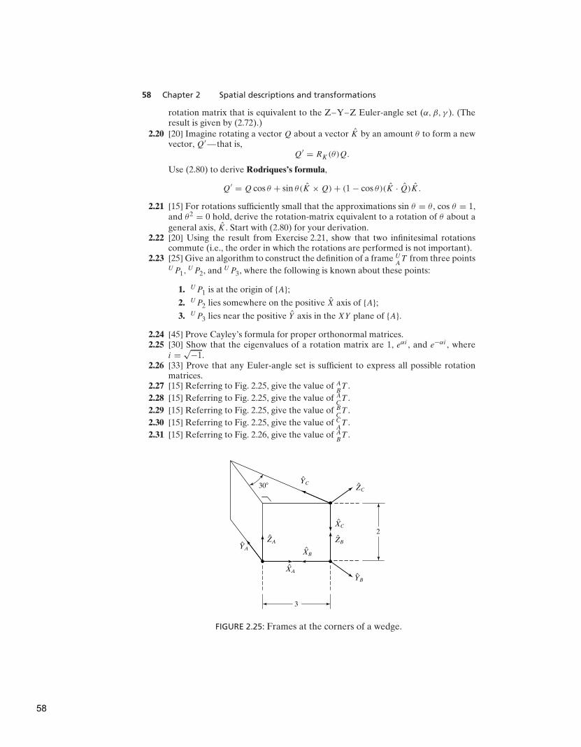
58 Chapter 2 Spatial descriptions and transformations
rotation matrix that is equivalent to the Z–Y–Z Euler-angle set (α, β, γ ). (Theresult is given by (2.72).)
2.20 [20] Imagine rotating a vectorQ about a vector K by an amount θ to form a newvector,Q′ —that is,
Q′ = RK(θ)Q.
Use (2.80) to derive Rodriques’s formula,
Q′ = Q cos θ + sin θ(K × Q)+ (1 − cos θ)(K · Q)K.
2.21 [15] For rotations sufficiently small that the approximations sin θ = θ , cos θ = 1,and θ2 = 0 hold, derive the rotation-matrix equivalent to a rotation of θ about ageneral axis, K . Start with (2.80) for your derivation.
2.22 [20] Using the result from Exercise 2.21, show that two infinitesimal rotationscommute (i.e., the order in which the rotations are performed is not important).
2.23 [25] Give an algorithm to construct the definition of a frame UAT from three points
UP1,UP2, and UP3, where the following is known about these points:
1. UP1 is at the origin of {A};2. UP2 lies somewhere on the positive X axis of {A};3. UP3 lies near the positive Y axis in the XY plane of {A}.
2.24 [45] Prove Cayley’s formula for proper orthonormal matrices.2.25 [30] Show that the eigenvalues of a rotation matrix are 1, eαi , and e−αi , where
i =√
−1.2.26 [33] Prove that any Euler-angle set is sufficient to express all possible rotation
matrices.2.27 [15] Referring to Fig. 2.25, give the value of A
BT .
2.28 [15] Referring to Fig. 2.25, give the value of ACT .
2.29 [15] Referring to Fig. 2.25, give the value of BCT .
2.30 [15] Referring to Fig. 2.25, give the value of CAT .
2.31 [15] Referring to Fig. 2.26, give the value of ABT .
ZC
XC
ZB
YB
XA
XB
ZAYA
YC
3
2
30
FIGURE 2.25: Frames at the corners of a wedge.
58

Programming exercise (Part 2) 59
ZCXC
ZB
YB
XA
ZA XB
YA
YC
3
2
36.9
4
FIGURE 2.26: Frames at the corners of a wedge.
2.32 [15] Referring to Fig. 2.26, give the value of ACT .
2.33 [15] Referring to Fig. 2.26, give the value of BCT .
2.34 [15] Referring to Fig. 2.26, give the value of CAT .
2.35 [20] Prove that the determinant of any rotation matrix is always equal to 1.2.36 [36] A rigid body moving in a plane (i.e., in 2-space) has three degrees of freedom.
A rigid body moving in 3-space has six degrees of freedom. Show that a body inN-space has 1
2 (N2 + N) degrees of freedom.
2.37 [15] Given
A
BT =
0.25 0.43 0.86 5.00.87 −0.50 0.00 −4.00.43 0.75 −0.50 3.00 0 0 1
,
what is the (2,4) element of BAT ?
2.38 [25] Imagine two unit vectors, v1 and v2, embedded in a rigid body. Note that, nomatter how the body is rotated, the geometric angle between these two vectors ispreserved (i.e., rigid-body rotation is an ‘‘angle-preserving’’ operation). Use thisfact to give a concise (four- or five-line) proof that the inverse of a rotation matrixmust equal its transpose and that a rotation matrix is orthonormal.
2.39 [37] Give an algorithm (perhaps in the form of a C program) that computes theunit quaternion corresponding to a given rotation matrix. Use (2.91) as startingpoint.
2.40 [33] Give an algorithm (perhaps in the form of a C program) that computes theZ–X–Z Euler angles corresponding to a given rotation matrix. See Appendix B.
2.41 [33] Give an algorithm (perhaps in the form of a C program) that computes theX–Y–X fixed angles corresponding to a given rotation matrix. See Appendix B.
PROGRAMMING EXERCISE (PART 2)
1. If your function library does not include an Atan2 function subroutine, write one.
2. To make a friendly user interface, we wish to describe orientations in the planarworld by a single angle, θ , instead of by a 2×2 rotation matrix. The user will always
59

60 Chapter 2 Spatial descriptions and transformations
communicate in terms of angle θ , but internally we will need the rotation-matrixform. For the position-vector part of a frame, the user will specify an x and ay value. So, we want to allow the user to specify a frame as a 3-tuple: (x, y, θ).Internally, we wish to use a 2 × 1 position vector and a 2 × 2 rotation matrix, so weneed conversion routines. Write a subroutine whose Pascal definition would begin
Procedure UTOI (VAR uform: vec3; VAR iform: frame);
where ‘‘UTOI’’ stands for ‘‘User form TO Internal form.’’ The first argument isthe 3-tuple (x, y, θ), and the second argument is of type ‘‘frame,’’ consists of a(2×1) position vector and a (2×2) rotation matrix. If you wish, you may representthe frame with a (3 × 3) homogeneous transform in which the third row is [0 0 1].The inverse routine will also be necessary:
Procedure ITOU (VAR iform: frame; VAR uform: vec3);
3. Write a subroutine to multiply two transforms together. Use the following proce-dure heading:
Procedure TMULT (VAR brela, crelb, crela: frame);
The first two arguments are inputs, and the third is an output. Note that the namesof the arguments document what the program does (brela = A
BT ).
4. Write a subroutine to invert a transform. Use the following procedure heading:
Procedure TINVERT (VAR brela, arelb: frame);
The first argument is the input, the second the output. Note that the names of thearguments document what the program does (brela =A
BT ).
5. The following frame definitions are given as known:
U
AT = [x y θ] = [11.0 − 1.0 30.0],
B
AT = [x y θ] = [0.0 7.0 45.0],
C
UT = [x y θ] = [−3.0 − 3.0 − 30.0].
These frames are input in the user representation [x, y, θ] (where θ is in degrees).Draw a frame diagram (like Fig. 2.15, only in 2-D) that qualitatively shows theirarrangement. Write a program that calls TMULT and TINVERT (defined inprogramming exercises 3 and 4) as many times as needed to solve for B
CT . Then
print out BCT in both internal and user representation.
MATLAB EXERCISE 2A
a) Using the Z–Y –X (α−β−γ ) Euler angle convention, write a MATLAB programto calculate the rotation matrix A
BR when the user enters the Euler angles α–β –γ .
Test for two examples:
i) α = 10◦, β = 20
◦, γ = 30
◦.
ii) α = 30◦, β = 90
◦, γ = −55
◦.
For case (i), demonstrate the six constraints for unitary orthonormal rotationmatrices (i.e., there are nine numbers in a 3 × 3 matrix, but only three areindependent). Also, demonstrate the beautiful property, B
AR = A
BR−1 = A
BRT ,
for case i.
60
MATLAB Exercise 2B 61
b) Write a MATLAB program to calculate the Euler angles α–β –γ when the userenters the rotation matrix A
BR (the inverse problem). Calculate both possible
solutions. Demonstrate this inverse solution for the two cases from part (a). Usea circular check to verify your results (i.e., enter Euler angles in code a from part(a); take the resulting rotation matrix A
BR, and use this as the input to code b; you
get two sets of answers—one should be the original user input, and the second canbe verified by once again using the code in part (a).
c) For a simple rotation of β about the Y axis only, for β = 20◦
and BP = {1 0 1 }T ,calculate AP ; demonstrate with a sketch that your results are correct.
d) Check all results, by means of the Corke MATLAB Robotics Toolbox. Try thefunctions rpy2tr(), tr2rpy(), rotx(), roty(), and rotz().
MATLAB EXERCISE 2B
a) Write a MATLAB program to calculate the homogeneous transformation matrixABT when the user enters Z–Y –X Euler angles α − β − γ and the position vector
APB . Test for two examples:
i) α = 10◦, β = 20
◦, γ = 30
◦, and APB = {1 2 3 }T .
ii) For β = 20◦
(α = γ = 0◦), APB = {3 0 1 }T .
b) For β = 20◦
(α = γ = 0◦), APB = {3 0 1}T , and BP = {1 0 1}T , use MATLAB to
calculate AP ; demonstrate with a sketch that your results are correct. Also, usingthe same numbers, demonstrate all three interpretations of the homogeneoustransformation matrix—the (b) assignment is the second interpretation, transformmapping.
c) Write a MATLAB program to calculate the inverse homogeneous transformationmatrix A
BT −1 = B
AT , using the symbolic formula. Compare your result with a
numerical MATLAB function (e.g., inv). Demonstrate that both methods yieldcorrect results (i.e., A
BT A
BT −1 = A
BT −1 A
BT = I4). Demonstrate this for examples (i)
and (ii) from (a) above.
d) Define ABT to be the result from (a)(i) and B
CT to be the result from (a)(ii).
i) Calculate ACT , and show the relationship via a transform graph. Do the same
for CAT .
ii) Given ACT and B
CT from (d)(i)—assume you don’t know A
BT , calculate it, and
compare your result with the answer you know.
iii) Given ACT and A
BT from (d)(i)—assume you don’t know B
CT , calculate it, and
compare your result with the answer you know.
e) Check all results by means of the Corke MATLAB Robotics Toolbox. Tryfunctions rpy2tr() and transl().
61
C H A P T E R 3
Manipulator kinematics
3.1 INTRODUCTION
3.2 LINK DESCRIPTION
3.3 LINK-CONNECTION DESCRIPTION
3.4 CONVENTION FOR AFFIXING FRAMES TO LINKS
3.5 MANIPULATOR KINEMATICS
3.6 ACTUATOR SPACE, JOINT SPACE, AND CARTESIAN SPACE
3.7 EXAMPLES: KINEMATICS OF TWO INDUSTRIAL ROBOTS
3.8 FRAMES WITH STANDARD NAMES
3.9 WHERE IS THE TOOL?
3.10 COMPUTATIONAL CONSIDERATIONS
3.1 INTRODUCTION
Kinematics is the science of motion that treats the subject without regard to theforces that cause it. Within the science of kinematics, one studies the position, thevelocity, the acceleration, and all higher order derivatives of the position variables(with respect to time or any other variable(s)). Hence, the study of the kinematics ofmanipulators refers to all the geometrical and time-based properties of the motion.The relationships between these motions and the forces and torques that cause themconstitute the problem of dynamics, which is the subject of Chapter 6.
In this chapter, we consider position and orientation of the manipulatorlinkages in static situations. In Chapters 5 and 6, we will consider the kinematicswhen velocities and accelerations are involved.
In order to deal with the complex geometry of a manipulator, we will affixframes to the various parts of the mechanism and then describe the relationshipsbetween these frames. The study of manipulator kinematics involves, among otherthings, how the locations of these frames change as the mechanism articulates. Thecentral topic of this chapter is a method to compute the position and orientation ofthe manipulator’s end-effector relative to the base of the manipulator as a functionof the joint variables.
3.2 LINK DESCRIPTION
A manipulator may be thought of as a set of bodies connected in a chain by joints.These bodies are called links. Joints form a connection between a neighboring pairof links. The term lower pair is used to describe the connection between a pair of
From Chapter 3 of Introduction to Robotics: Mechanics and Control, Third Edition. John J. Craig.
Copyright © 2005 by Pearson Education, Inc. All rights reserved.
62
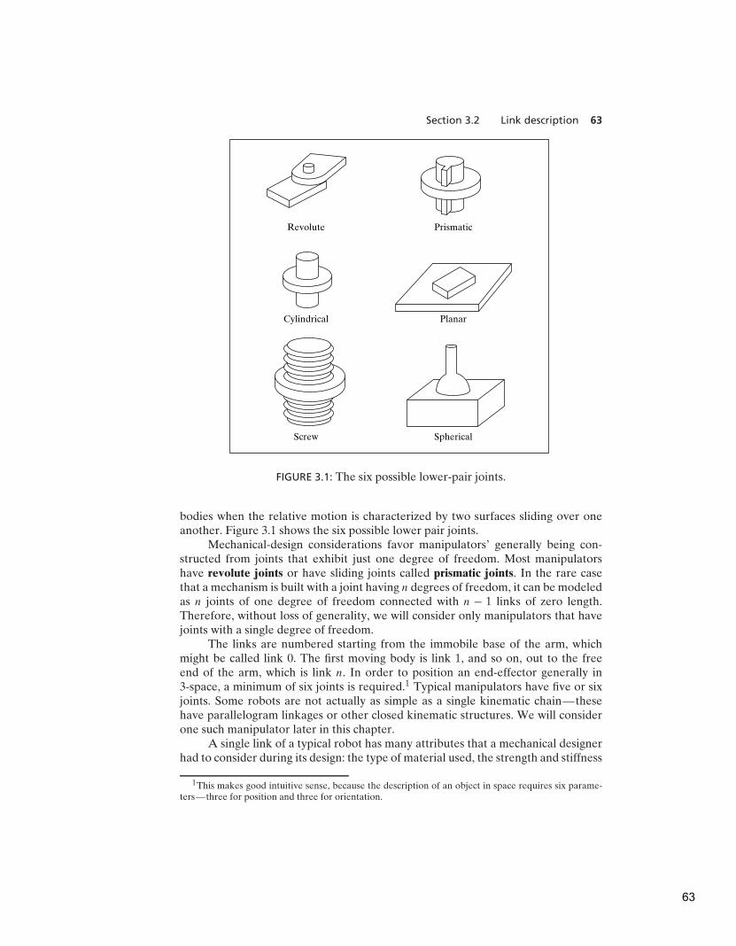
Section 3.2 Link description 63
Revolute
Cylindrical
Screw
Prismatic
Planar
Spherical
FIGURE 3.1: The six possible lower-pair joints.
bodies when the relative motion is characterized by two surfaces sliding over oneanother. Figure 3.1 shows the six possible lower pair joints.
Mechanical-design considerations favor manipulators’ generally being con-structed from joints that exhibit just one degree of freedom. Most manipulatorshave revolute joints or have sliding joints called prismatic joints. In the rare casethat a mechanism is built with a joint having n degrees of freedom, it can be modeledas n joints of one degree of freedom connected with n − 1 links of zero length.Therefore, without loss of generality, we will consider only manipulators that havejoints with a single degree of freedom.
The links are numbered starting from the immobile base of the arm, whichmight be called link 0. The first moving body is link 1, and so on, out to the freeend of the arm, which is link n. In order to position an end-effector generally in3-space, a minimum of six joints is required.1 Typical manipulators have five or sixjoints. Some robots are not actually as simple as a single kinematic chain—thesehave parallelogram linkages or other closed kinematic structures. We will considerone such manipulator later in this chapter.
A single link of a typical robot has many attributes that a mechanical designerhad to consider during its design: the type of material used, the strength and stiffness
1This makes good intuitive sense, because the description of an object in space requires six parame-ters—three for position and three for orientation.
63
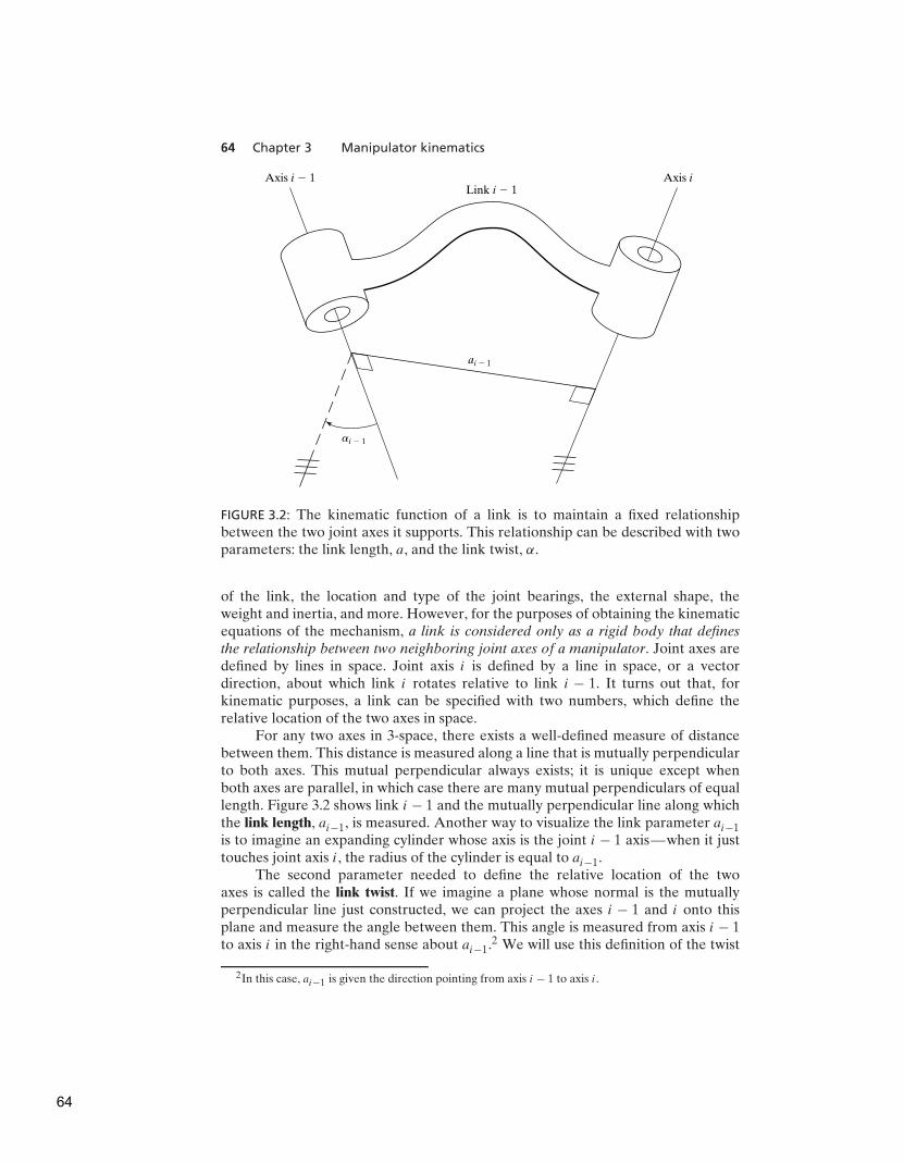
64 Chapter 3 Manipulator kinematics
Link i � 1
ai � 1
ai � 1
Axis i � 1 Axis i
FIGURE 3.2: The kinematic function of a link is to maintain a fixed relationshipbetween the two joint axes it supports. This relationship can be described with twoparameters: the link length, a, and the link twist, α.
of the link, the location and type of the joint bearings, the external shape, theweight and inertia, and more. However, for the purposes of obtaining the kinematicequations of the mechanism, a link is considered only as a rigid body that defines
the relationship between two neighboring joint axes of a manipulator. Joint axes aredefined by lines in space. Joint axis i is defined by a line in space, or a vectordirection, about which link i rotates relative to link i − 1. It turns out that, forkinematic purposes, a link can be specified with two numbers, which define therelative location of the two axes in space.
For any two axes in 3-space, there exists a well-defined measure of distancebetween them. This distance is measured along a line that is mutually perpendicularto both axes. This mutual perpendicular always exists; it is unique except whenboth axes are parallel, in which case there are many mutual perpendiculars of equallength. Figure 3.2 shows link i − 1 and the mutually perpendicular line along whichthe link length, ai−1, is measured. Another way to visualize the link parameter ai−1is to imagine an expanding cylinder whose axis is the joint i − 1 axis—when it justtouches joint axis i, the radius of the cylinder is equal to ai−1.
The second parameter needed to define the relative location of the twoaxes is called the link twist. If we imagine a plane whose normal is the mutuallyperpendicular line just constructed, we can project the axes i − 1 and i onto thisplane and measure the angle between them. This angle is measured from axis i − 1to axis i in the right-hand sense about ai−1.2 We will use this definition of the twist
2In this case, ai−1 is given the direction pointing from axis i − 1 to axis i.
64

Section 3.3 Link-connection description 65
45
2 in. 2 in.Bearing “A” Bearing “B”
3 in.
2 in. 2 in.5 in.
FIGURE 3.3: A simple link that supports two revolute axes.
of link i − 1, αi−1. In Fig. 3.2, αi−1 is indicated as the angle between axis i − 1 andaxis i. (The lines with the triple hash marks are parallel.) In the case of intersectingaxes, twist is measured in the plane containing both axes, but the sense of αi−1 islost. In this special case, one is free to assign the sign of αi−1 arbitrarily.
You should convince yourself that these two parameters, length and twist, asdefined above, can be used to define the relationship between any two lines (in thiscase axes) in space.
EXAMPLE 3.1
Figure 3.3 shows the mechanical drawings of a robot link. If this link is used in arobot, with bearing ‘‘A’’ used for the lower-numbered joint, give the length andtwist of this link. Assume that holes are centered in each bearing.
By inspection, the common perpendicular lies right down the middle ofthe metal bar connecting the bearings, so the link length is 7 inches. The end viewactually shows a projection of the bearings onto the plane whose normal is the mutualperpendicular. Link twist is measured in the right-hand sense about the commonperpendicular from axis i − 1 to axis i, so, in this example, it is clearly +45 degrees.
3.3 LINK-CONNECTION DESCRIPTION
The problem of connecting the links of a robot together is again one filled withmany questions for the mechanical designer to resolve. These include the strengthof the joint, its lubrication, and the bearing and gearing mounting. However, forthe investigation of kinematics, we need only worry about two quantities, which willcompletely specify the way in which links are connected together.
65
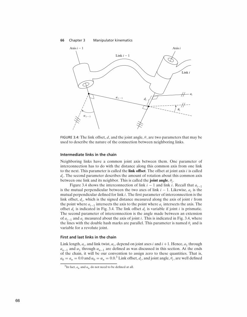
66 Chapter 3 Manipulator kinematics
ai
ui
Axis i � 1
Link i � 1
Link i
Axis i
di
a i � 1
a i � 1
FIGURE 3.4: The link offset, d, and the joint angle, θ , are two parameters that may beused to describe the nature of the connection between neighboring links.
Intermediate links in the chain
Neighboring links have a common joint axis between them. One parameter ofinterconnection has to do with the distance along this common axis from one linkto the next. This parameter is called the link offset. The offset at joint axis i is calleddi . The second parameter describes the amount of rotation about this common axisbetween one link and its neighbor. This is called the joint angle, θi .
Figure 3.4 shows the interconnection of link i − 1 and link i. Recall that ai−1is the mutual perpendicular between the two axes of link i − 1. Likewise, ai is themutual perpendicular defined for link i. The first parameter of interconnection is thelink offset, di , which is the signed distance measured along the axis of joint i fromthe point where ai−1 intersects the axis to the point where ai intersects the axis. Theoffset di is indicated in Fig. 3.4. The link offset di is variable if joint i is prismatic.The second parameter of interconnection is the angle made between an extensionof ai−1 and ai measured about the axis of joint i. This is indicated in Fig. 3.4, wherethe lines with the double hash marks are parallel. This parameter is named θi and isvariable for a revolute joint.
First and last links in the chain
Link length, ai , and link twist, αi , depend on joint axes i and i +1. Hence, a1 throughan−1 and α1 through αn−1 are defined as was discussed in this section. At the endsof the chain, it will be our convention to assign zero to these quantities. That is,a0 = an = 0.0 and α0 = αn = 0.0.3 Link offset, di , and joint angle, θi , are well defined
3In fact, an and αn do not need to be defined at all.
66

Section 3.4 Convention for affixing frames to links 67
for joints 2 through n − 1 according to the conventions discussed in this section. Ifjoint 1 is revolute, the zero position for θ1 may be chosen arbitrarily; d1 = 0.0 willbe our convention. Similarly, if joint 1 is prismatic, the zero position of d1 may bechosen arbitrarily; θ1 = 0.0 will be our convention. Exactly the same statementsapply to joint n.
These conventions have been chosen so that, in a case where a quantity couldbe assigned arbitrarily, a zero value is assigned so that later calculations will be assimple as possible.
Link parameters
Hence, any robot can be described kinematically by giving the values of fourquantities for each link. Two describe the link itself, and two describe the link’sconnection to a neighboring link. In the usual case of a revolute joint, θi is calledthe joint variable, and the other three quantities would be fixed link parameters.For prismatic joints, di is the joint variable, and the other three quantities are fixedlink parameters. The definition of mechanisms by means of these quantities is aconvention usually called the Denavit–Hartenberg notation [1].4 Other methods ofdescribing mechanisms are available, but are not presented here.
At this point, we could inspect any mechanism and determine theDenavit–Hartenberg parameters that describe it. For a six-jointed robot, 18 num-bers would be required to describe the fixed portion of its kinematics completely.In the case of a six-jointed robot with all revolute joints, the 18 numbers are in theform of six sets of (αi , αi , di).
EXAMPLE 3.2
Two links, as described in Fig. 3.3, are connected as links 1 and 2 of a robot. Joint 2is composed of a ‘‘B’’ bearing of link 1 and an ‘‘A’’ bearing of link 2, arranged sothat the flat surfaces of the ‘‘A’’ and ‘‘B’’ bearings lie flush against each other. Whatis d2?
The link offset d2 is the offset at joint 2, which is the distance, measured alongthe joint 2 axis, between the mutual perpendicular of link 1 and that of link 2. Fromthe drawings in Fig. 3.3, this is 2.5 inches.
Before introducing more examples, we will define a convention for attachinga frame to each link of the manipulator.
3.4 CONVENTION FOR AFFIXING FRAMES TO LINKS
In order to describe the location of each link relative to its neighbors, we define aframe attached to each link. The link frames are named by number according to thelink to which they are attached. That is, frame {i} is attached rigidly to link i.
4Note that many related conventions go by the name Denavit–Hartenberg, but differ in a few details.For example, the version used in this book differs from some of the robotic literature in the manner offrame numbering. Unlike some other conventions, in this book frame {i} is attached to link i and has itsorigin lying on joint axis i.
67
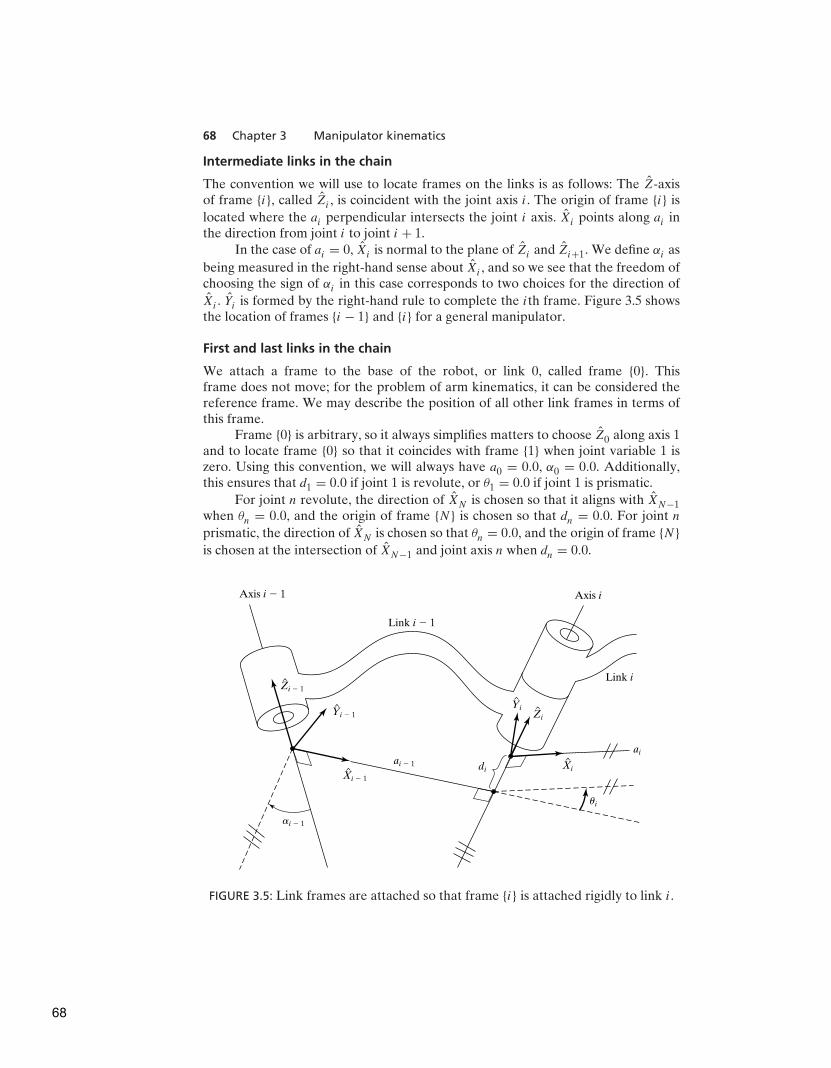
68 Chapter 3 Manipulator kinematics
Intermediate links in the chain
The convention we will use to locate frames on the links is as follows: The Z-axisof frame {i}, called Zi , is coincident with the joint axis i. The origin of frame {i} is
located where the ai perpendicular intersects the joint i axis. Xi points along ai inthe direction from joint i to joint i + 1.
In the case of ai = 0, Xi is normal to the plane of Zi and Zi+1. We define αi as
being measured in the right-hand sense about Xi , and so we see that the freedom ofchoosing the sign of αi in this case corresponds to two choices for the direction of
Xi . Yi is formed by the right-hand rule to complete the ith frame. Figure 3.5 showsthe location of frames {i − 1} and {i} for a general manipulator.
First and last links in the chain
We attach a frame to the base of the robot, or link 0, called frame {0}. Thisframe does not move; for the problem of arm kinematics, it can be considered thereference frame. We may describe the position of all other link frames in terms ofthis frame.
Frame {0} is arbitrary, so it always simplifies matters to choose Z0 along axis 1and to locate frame {0} so that it coincides with frame {1} when joint variable 1 iszero. Using this convention, we will always have a0 = 0.0, α0 = 0.0. Additionally,this ensures that d1 = 0.0 if joint 1 is revolute, or θ1 = 0.0 if joint 1 is prismatic.
For joint n revolute, the direction of XN is chosen so that it aligns with XN−1when θn = 0.0, and the origin of frame {N} is chosen so that dn = 0.0. For joint n
prismatic, the direction of XN is chosen so that θn = 0.0, and the origin of frame {N}
is chosen at the intersection of XN−1 and joint axis n when dn = 0.0.
ai
ui
Axis i � 1
Link i � 1
Link i
Axis i
diai � 1
ai � 1
XiXi � 1
Yi � 1
Zi � 1
Zi
Yi
FIGURE 3.5: Link frames are attached so that frame {i} is attached rigidly to link i.
68

Section 3.4 Convention for affixing frames to links 69
Summary of the link parameters in terms of the link frames
If the link frames have been attached to the links according to our convention, thefollowing definitions of the link parameters are valid:
ai = the distance f rom Zi to Zi+1 measured along Xi;
αi = the angle f rom Zi to Zi+1 measured about Xi;
di = the distance f rom Xi−1 to Xi measured along Zi; and
θi = the angle f rom Xi−1 to Xi measured about Zi .
We usually choose ai > 0, because it corresponds to a distance; however, αi ,di , and θi are signed quantities.
A final note on uniqueness is warranted. The convention outlined above doesnot result in a unique attachment of frames to links. First of all, when we first alignthe Zi axis with joint axis i, there are two choices of direction in which to point
Zi . Furthermore, in the case of intersecting joint axes (i.e., ai = 0), there are two
choices for the direction of Xi , corresponding to the choice of signs for the normal
to the plane containing Zi and Zi+1. When axes i and i + 1 are parallel, the choiceof origin location for {i} is arbitrary (though generally chosen in order to cause di tobe zero). Also, when prismatic joints are present, there is quite a bit of freedom inframe assignment. (See also Example 3.5.)
Summary of link-frame attachment procedure
The following is a summary of the procedure to follow when faced with a newmechanism, in order to properly attach the link frames:
1. Identify the joint axes and imagine (or draw) infinite lines along them. Forsteps 2 through 5 below, consider two of these neighboring lines (at axes i andi + 1).
2. Identify the common perpendicular between them, or point of intersection.At the point of intersection, or at the point where the common perpendicularmeets the ith axis, assign the link-frame origin.
3. Assign the Zi axis pointing along the ith joint axis.
4. Assign the Xi axis pointing along the common perpendicular, or, if the axes
intersect, assign Xi to be normal to the plane containing the two axes.
5. Assign the Yi axis to complete a right-hand coordinate system.
6. Assign {0} to match {1} when the first joint variable is zero. For {N}, choose anorigin location and XN direction freely, but generally so as to cause as manylinkage parameters as possible to become zero.
EXAMPLE 3.3
Figure 3.6(a) shows a three-link planar arm. Because all three joints are revolute,this manipulator is sometimes called an RRR (or 3R) mechanism. Fig. 3.6(b) is aschematic representation of the same manipulator. Note the double hash marks
69
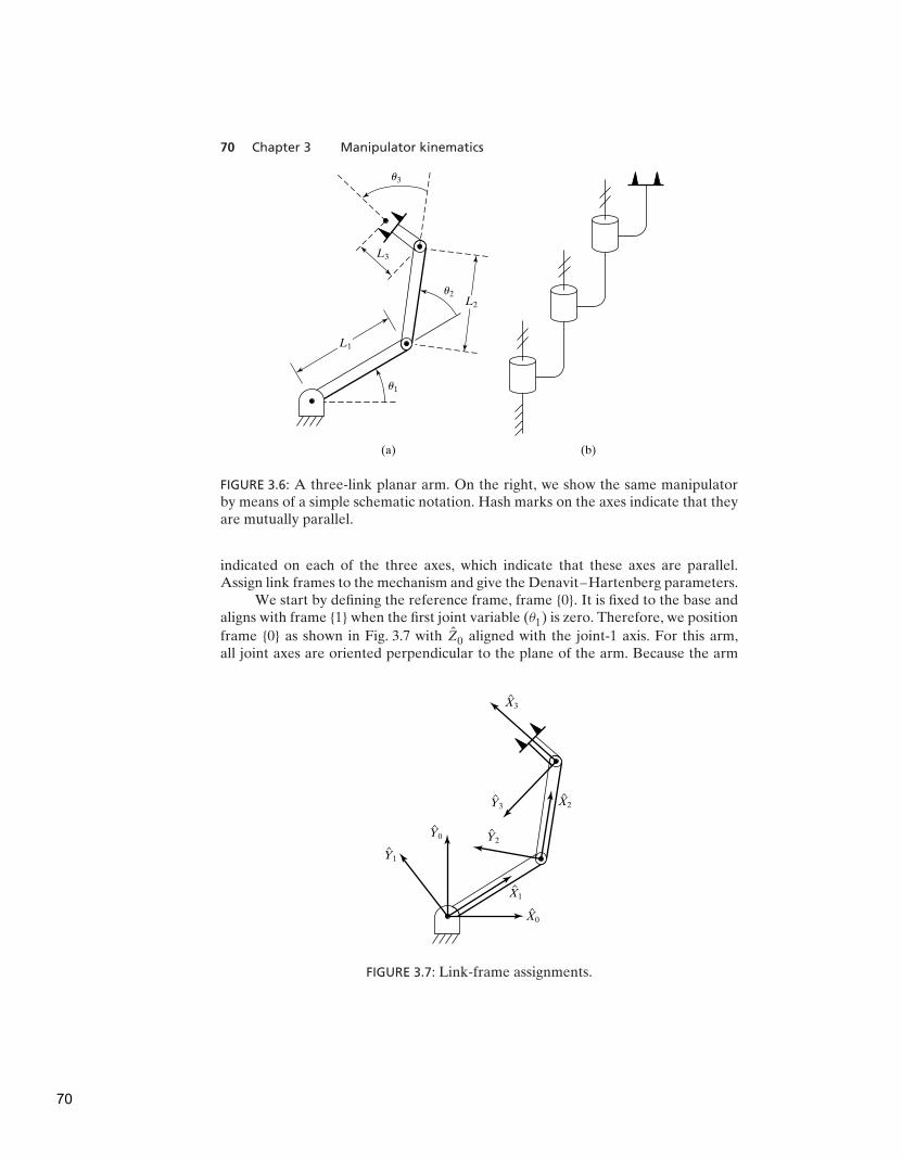
70 Chapter 3 Manipulator kinematics
L3
u3
L1
u1
u2L2
(a) (b)
FIGURE 3.6: A three-link planar arm. On the right, we show the same manipulatorby means of a simple schematic notation. Hash marks on the axes indicate that theyare mutually parallel.
indicated on each of the three axes, which indicate that these axes are parallel.Assign link frames to the mechanism and give the Denavit–Hartenberg parameters.
We start by defining the reference frame, frame {0}. It is fixed to the base andaligns with frame {1} when the first joint variable (θ1) is zero. Therefore, we position
frame {0} as shown in Fig. 3.7 with Z0 aligned with the joint-1 axis. For this arm,all joint axes are oriented perpendicular to the plane of the arm. Because the arm
X2
X0
X1
X3
Y1
Y0 Y2
Y3
FIGURE 3.7: Link-frame assignments.
70
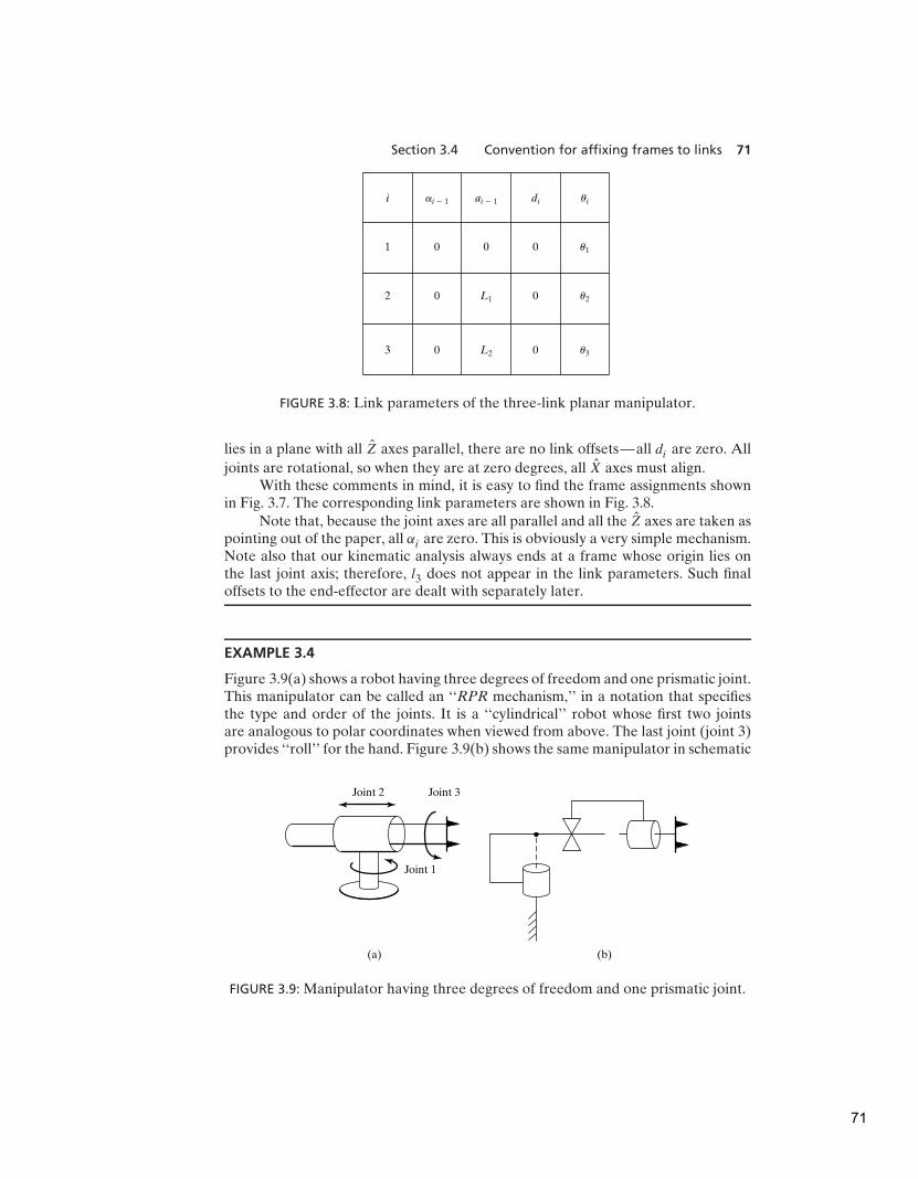
Section 3.4 Convention for affixing frames to links 71
i ai � 1 ai � 1 di ui
1 0 0 0 u1
2 0 L1 0 u2
3 0 L2 0 u3
FIGURE 3.8: Link parameters of the three-link planar manipulator.
lies in a plane with all Z axes parallel, there are no link offsets—all di are zero. All
joints are rotational, so when they are at zero degrees, all X axes must align.With these comments in mind, it is easy to find the frame assignments shown
in Fig. 3.7. The corresponding link parameters are shown in Fig. 3.8.Note that, because the joint axes are all parallel and all the Z axes are taken as
pointing out of the paper, all αi are zero. This is obviously a very simple mechanism.Note also that our kinematic analysis always ends at a frame whose origin lies onthe last joint axis; therefore, l3 does not appear in the link parameters. Such finaloffsets to the end-effector are dealt with separately later.
EXAMPLE 3.4
Figure 3.9(a) shows a robot having three degrees of freedom and one prismatic joint.This manipulator can be called an ‘‘RPR mechanism,’’ in a notation that specifiesthe type and order of the joints. It is a ‘‘cylindrical’’ robot whose first two jointsare analogous to polar coordinates when viewed from above. The last joint (joint 3)provides ‘‘roll’’ for the hand. Figure 3.9(b) shows the same manipulator in schematic
Joint 1
Joint 2 Joint 3
(a) (b)
FIGURE 3.9: Manipulator having three degrees of freedom and one prismatic joint.
71
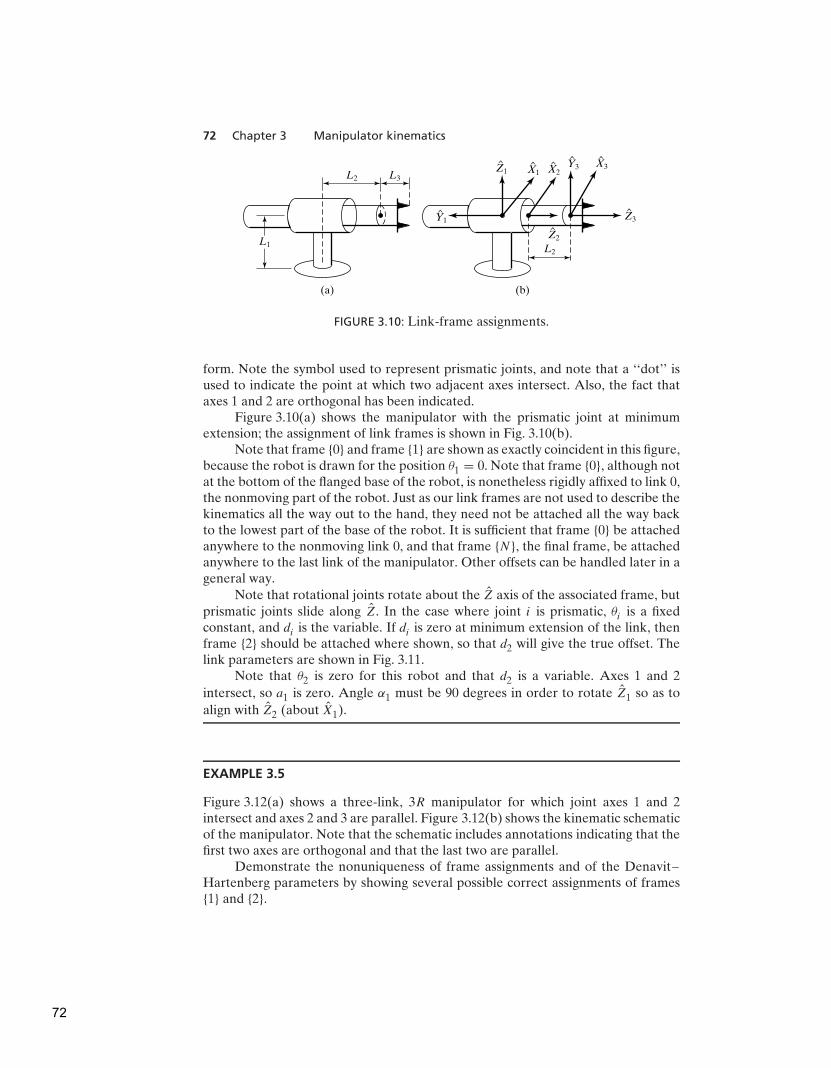
72 Chapter 3 Manipulator kinematics
(a) (b)
L2 L3
L1L2
X3X2X1
Y1
Y3
Z2
Z3
Z1
FIGURE 3.10: Link-frame assignments.
form. Note the symbol used to represent prismatic joints, and note that a ‘‘dot’’ isused to indicate the point at which two adjacent axes intersect. Also, the fact thataxes 1 and 2 are orthogonal has been indicated.
Figure 3.10(a) shows the manipulator with the prismatic joint at minimumextension; the assignment of link frames is shown in Fig. 3.10(b).
Note that frame {0} and frame {1} are shown as exactly coincident in this figure,because the robot is drawn for the position θ1 = 0. Note that frame {0}, although notat the bottom of the flanged base of the robot, is nonetheless rigidly affixed to link 0,the nonmoving part of the robot. Just as our link frames are not used to describe thekinematics all the way out to the hand, they need not be attached all the way backto the lowest part of the base of the robot. It is sufficient that frame {0} be attachedanywhere to the nonmoving link 0, and that frame {N}, the final frame, be attachedanywhere to the last link of the manipulator. Other offsets can be handled later in ageneral way.
Note that rotational joints rotate about the Z axis of the associated frame, butprismatic joints slide along Z. In the case where joint i is prismatic, θi is a fixedconstant, and di is the variable. If di is zero at minimum extension of the link, thenframe {2} should be attached where shown, so that d2 will give the true offset. Thelink parameters are shown in Fig. 3.11.
Note that θ2 is zero for this robot and that d2 is a variable. Axes 1 and 2
intersect, so a1 is zero. Angle α1 must be 90 degrees in order to rotate Z1 so as to
align with Z2 (about X1).
EXAMPLE 3.5
Figure 3.12(a) shows a three-link, 3R manipulator for which joint axes 1 and 2intersect and axes 2 and 3 are parallel. Figure 3.12(b) shows the kinematic schematicof the manipulator. Note that the schematic includes annotations indicating that thefirst two axes are orthogonal and that the last two are parallel.
Demonstrate the nonuniqueness of frame assignments and of the Denavit–Hartenberg parameters by showing several possible correct assignments of frames{1} and {2}.
72

Section 3.5 Manipulator kinematics 73
i ai � 1 ai � 1 di ui
1 0 0 0 u1
2 0 d2 0
3 0 0 L2 u3
90
FIGURE 3.11: Link parameters for the RPR manipulator of Example 3.4.
(a) (b)
L1
L2
FIGURE 3.12: Three-link, nonplanar manipulator.
Figure 3.13 shows two possible frame assignments and corresponding param-eters for the two possible choices of direction of Z2.
In general, when Zi and Zi+1 intersect, there are two choices for Xi . In thisexample, joint axes 1 and 2 intersect, so there are two choices for the direction ofX1. Figure 3.14 shows two more possible frame assignments, corresponding to the
second choice of X1.In fact, there are four more possibilities, corresponding to the preceding four
choices, but with Z1 pointing downward.
3.5 MANIPULATOR KINEMATICS
In this section, we derive the general form of the transformation that relatesthe frames attached to neighboring links. We then concatenate these individualtransformations to solve for the position and orientation of link n relative to link 0.
73

74 Chapter 3 Manipulator kinematics
Y1 Y1
a1 � 0
d1 � 0
a1 � �90
a1 � 0
d1 � 0
a2 � L2
d2 � L1
a2 � 0 u2 � �90 a1 � 90 u2 � 90
a2 � L2
d2 � �L1
a2 � 0
X2
X1
X2
X1
Y2
Y2
Z2
Z1
Z2
Z1
FIGURE 3.13: Two possible frame assignments.
a1 � 0
d1 � 0
a1 � 0
d1 � 0
a1 � 90 u2 � 90
a2 � L2
d2 � L1
a2 � 0 a1 � �90 u2 � �90
a2 � L2
d2 � �L1
a2 � 0
X2X1X2X1
Y2
Y2
Y1Y1
Z2
Z1
Z2
Z1
FIGURE 3.14: Two more possible frame assignments.
Derivation of link transformations
We wish to construct the transform that defines frame {i} relative to the frame {i−1}.In general, this transformation will be a function of the four link parameters. Forany given robot, this transformation will be a function of only one variable, the otherthree parameters being fixed by mechanical design. By defining a frame for eachlink, we have broken the kinematics problem into n subproblems. In order to solveeach of these subproblems, namely i−1
iT , we will further break each subproblem
into four subsubproblems. Each of these four transformations will be a function of
one link parameter only and will be simple enough that we can write down its form
by inspection. We begin by defining three intermediate frames for each link—{P },{Q}, and {R}.
Figure 3.15 shows the same pair of joints as before with frames {P }, {Q}, and{R} defined. Note that only the X and Z axes are shown for each frame, to makethe drawing clearer. Frame {R} differs from frame {i − 1} only by a rotation of αi−1.
74
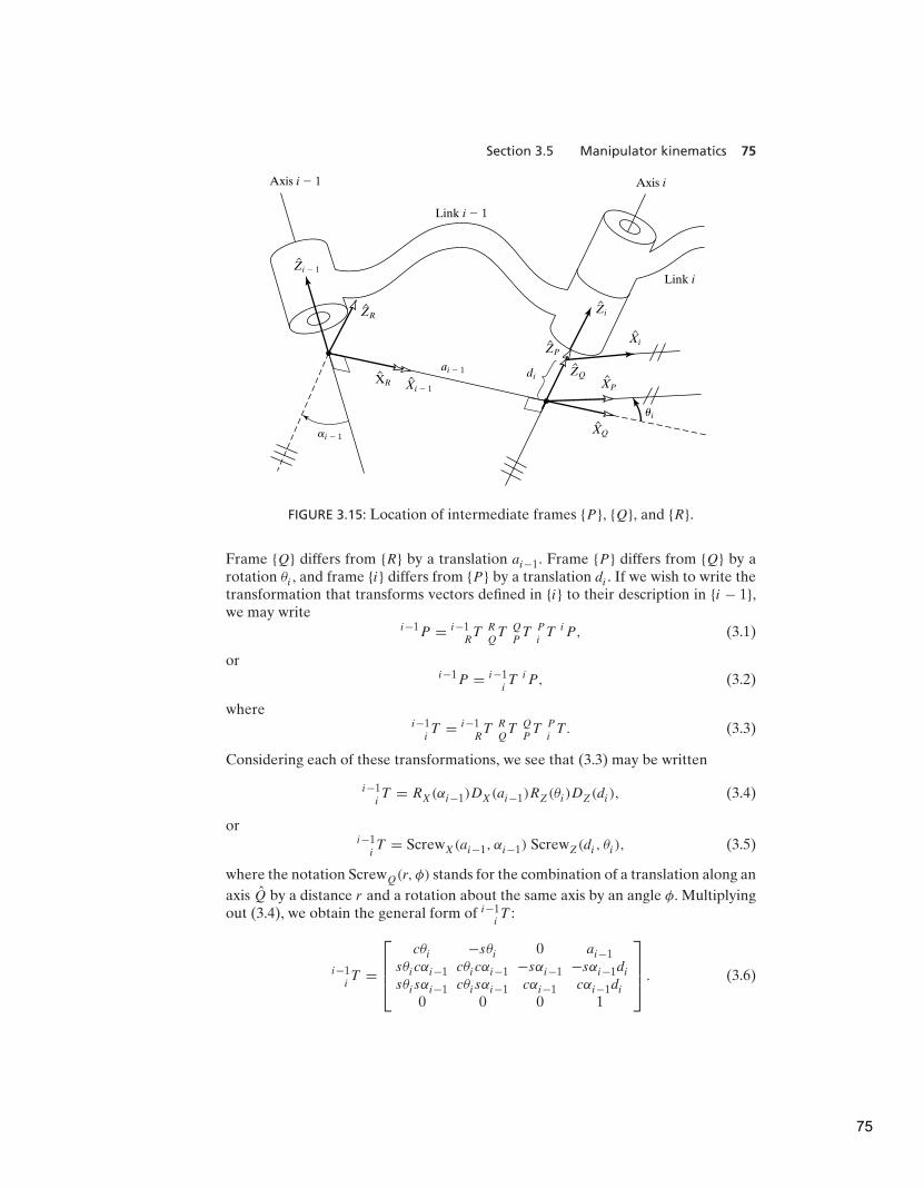
Section 3.5 Manipulator kinematics 75
ui
Axis i � 1
Link i � 1
Link i
Axis i
diai � 1
ai � 1
Xi
XP
XQ
Xi � 1XR
ZQ
ZP
Zi
Zi � 1
ZR
FIGURE 3.15: Location of intermediate frames {P }, {Q}, and {R}.
Frame {Q} differs from {R} by a translation ai−1. Frame {P } differs from {Q} by arotation θi , and frame {i} differs from {P } by a translation di . If we wish to write thetransformation that transforms vectors defined in {i} to their description in {i − 1},we may write
i−1P = i−1RT R
QT Q
PT P
iT iP, (3.1)
ori−1P = i−1
iT iP, (3.2)
wherei−1
iT = i−1
RT R
QT Q
PT P
iT . (3.3)
Considering each of these transformations, we see that (3.3) may be written
i−1iT = RX(αi−1)DX(ai−1)RZ(θi)DZ(di), (3.4)
ori−1
iT = ScrewX(ai−1, αi−1) ScrewZ(di, θi), (3.5)
where the notation ScrewQ(r, φ) stands for the combination of a translation along an
axis Q by a distance r and a rotation about the same axis by an angle φ. Multiplyingout (3.4), we obtain the general form of i−1
iT :
i−1iT =
cθi −sθi 0 ai−1sθicαi−1 cθicαi−1 −sαi−1 −sαi−1di
sθisαi−1 cθisαi−1 cαi−1 cαi−1di
0 0 0 1
. (3.6)
75

76 Chapter 3 Manipulator kinematics
EXAMPLE 3.6
Using the link parameters shown in Fig. 3.11 for the robot of Fig. 3.9, compute theindividual transformations for each link.
Substituting the parameters into (3.6), we obtain
01T =
cθ1 −sθ1 0 0sθ1 cθ1 0 00 0 1 00 0 0 1
,
12T =
1 0 0 00 0 −1 −d20 1 0 00 0 0 1
, (3.7)
23T =
cθ3 −sθ3 0 0sθ3 cθ3 0 00 0 1 l20 0 0 1
.
Once having derived these link transformations, we will find it a good idea to checkthem against common sense. For example, the elements of the fourth column ofeach transform should give the coordinates of the origin of the next higher frame.
Concatenating link transformations
Once the link frames have been defined and the corresponding link parametersfound, developing the kinematic equations is straightforward. From the values of thelink parameters, the individual link-transformation matrices can be computed. Then,the link transformations can be multiplied together to find the single transformationthat relates frame {N} to frame {0}:
0NT = 0
1T 1
2T 2
3T . . .N−1
NT . (3.8)
This transformation, 0NT , will be a function of all n joint variables. If the robot’s
joint-position sensors are queried, the Cartesian position and orientation of the lastlink can be computed by 0
NT .
3.6 ACTUATOR SPACE, JOINT SPACE, AND CARTESIAN SPACE
The position of all the links of a manipulator of n degrees of freedom can bespecified with a set of n joint variables. This set of variables is often referred to asthe n× 1 joint vector. The space of all such joint vectors is referred to as joint space.Thus far in this chapter, we have been concerned with computing the Cartesianspace description from knowledge of the joint-space description. We use the termCartesian space when position is measured along orthogonal axes and orientationis measured according to any of the conventions outlined in Chapter 2. Sometimes,the terms task-oriented space and operational space are used for what we will callCartesian space.
76

Section 3.7 Examples: kinematics of two industrial robots 77
Actuatorspace
Jointspace
Cartesianspace
FIGURE 3.16: Mappings between kinematic descriptions.
So far, we have implicitly assumed that each kinematic joint is actuated directlyby some sort of actuator. However, in the case of many industrial robots, this is not so.For example, sometimes two actuators work together in a differential pair to move asingle joint, or sometimes a linear actuator is used to rotate a revolute joint, throughthe use of a four-bar linkage. In these cases, it is helpful to consider the notion ofactuator positions. The sensors that measure the position of the manipulator areoften located at the actuators, so some computations must be performed to realizethe joint vector as a function of a set of actuator values, or actuator vector.
As is indicated in Fig. 3.16, there are three representations of a manipulator’sposition and orientation: descriptions in actuator space, in joint space, and inCartesian space. In this chapter, we are concerned with the mappings betweenrepresentations, as indicated by the solid arrows in Fig. 3.16. In Chapter 4, we willconsider the inverse mappings, indicated by the dashed arrows.
The ways in which actuators might be connected to move a joint are quitevaried; they might be catalogued, but we will not do so here. For each robot wedesign or seek to analyze, the correspondence between actuator positions and jointpositions must be solved. In the next section, we will solve an example problem foran industrial robot.
3.7 EXAMPLES: KINEMATICS OF TWO INDUSTRIAL ROBOTS
Current industrial robots are available in many different kinematic configurations [2],[3]. In this section, we work out the kinematics of two typical industrial robots. Firstwe consider the Unimation PUMA 560, a rotary-joint manipulator with six degreesof freedom. We will solve for the kinematic equations as functions of the joint angles.For this example, we will skip the additional problem of the relationship betweenactuator space and joint space. Second, we consider the Yasukawa Motoman L-3, arobot with five degrees of freedom and rotary joints. This example is done in detail,including the actuator-to-joint transformations. This example may be skipped onfirst reading of the book.
The PUMA 560
The Unimation PUMA 560 (Fig. 3.17) is a robot with six degrees of freedomand all rotational joints (i.e., it is a 6R mechanism). It is shown in Fig. 3.18, with
77
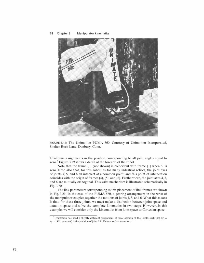
78 Chapter 3 Manipulator kinematics
FIGURE 3.17: The Unimation PUMA 560. Courtesy of Unimation Incorporated,Shelter Rock Lane, Danbury, Conn.
link-frame assignments in the position corresponding to all joint angles equal tozero.5 Figure 3.19 shows a detail of the forearm of the robot.
Note that the frame {0} (not shown) is coincident with frame {1} when θ1 iszero. Note also that, for this robot, as for many industrial robots, the joint axesof joints 4, 5, and 6 all intersect at a common point, and this point of intersectioncoincides with the origin of frames {4}, {5}, and {6}. Furthermore, the joint axes 4, 5,and 6 are mutually orthogonal. This wrist mechanism is illustrated schematically inFig. 3.20.
The link parameters corresponding to this placement of link frames are shownin Fig. 3.21. In the case of the PUMA 560, a gearing arrangement in the wrist ofthe manipulator couples together the motions of joints 4, 5, and 6. What this meansis that, for these three joints, we must make a distinction between joint space andactuator space and solve the complete kinematics in two steps. However, in thisexample, we will consider only the kinematics from joint space to Cartesian space.
5Unimation has used a slightly different assignment of zero location of the joints, such that θ∗3
=
θ3 − 180◦, where θ∗3
is the position of joint 3 in Unimation’s convention.
78
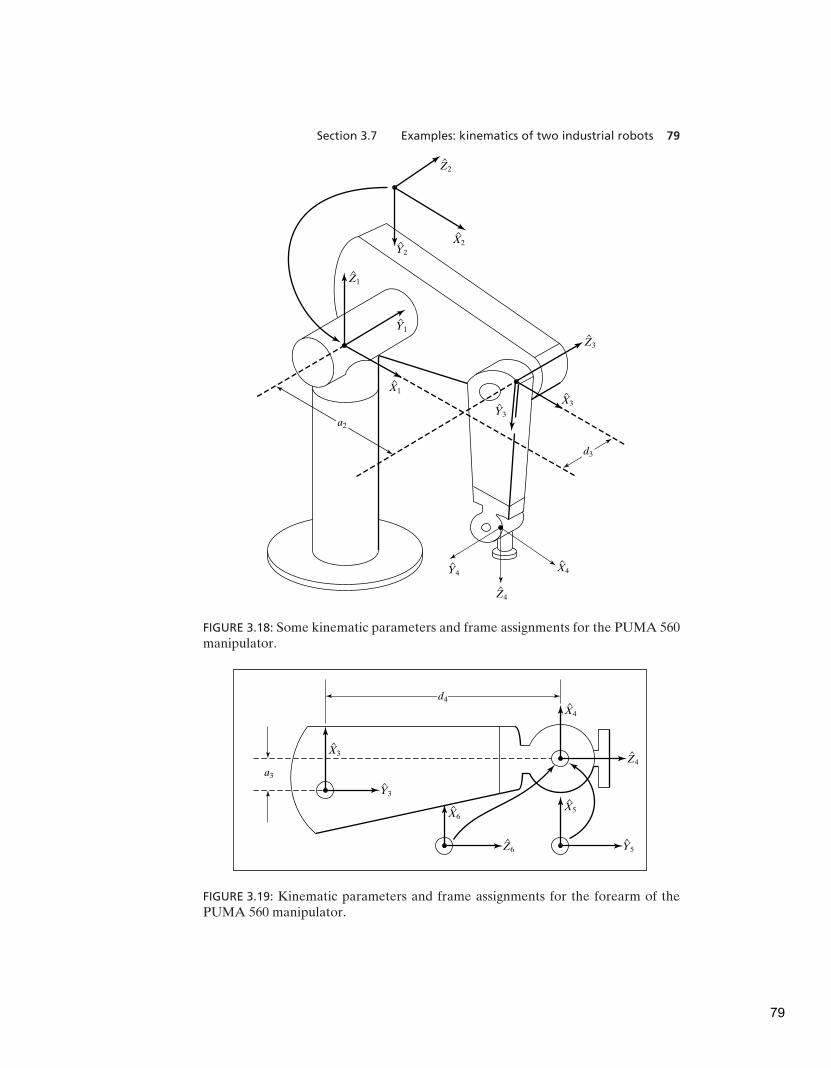
Section 3.7 Examples: kinematics of two industrial robots 79
a2
d3
X1
X2
Y4
Y3
Y1
Y2
Z4
X4
X3
Z3
Z1
Z2
FIGURE 3.18: Some kinematic parameters and frame assignments for the PUMA 560manipulator.
X3
X6
X4
X5
Z6
Z4
Y3
Y5
a3
d4
FIGURE 3.19: Kinematic parameters and frame assignments for the forearm of thePUMA 560 manipulator.
79
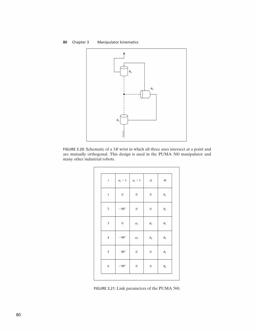
80 Chapter 3 Manipulator kinematics
u4
u5
u6
FIGURE 3.20: Schematic of a 3R wrist in which all three axes intersect at a point andare mutually orthogonal. This design is used in the PUMA 560 manipulator andmany other industrial robots.
6
5
4
3
2
1
i
0
0
ai � 1
0
0
a3
a2
0
0
ai � 1
0
0
d4
d3
0
0
di
u6
u5
u4
u3
u2
u1
ui
�90
90
�90
�90
FIGURE 3.21: Link parameters of the PUMA 560.
80
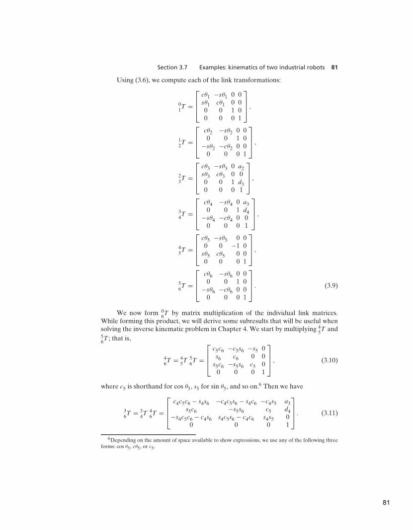
Section 3.7 Examples: kinematics of two industrial robots 81
Using (3.6), we compute each of the link transformations:
01T =
cθ1 −sθ1 0 0sθ1 cθ1 0 00 0 1 00 0 0 1
,
12T =
cθ2 −sθ2 0 00 0 1 0
−sθ2 −cθ2 0 00 0 0 1
,
23T =
cθ3 −sθ3 0 a2sθ3 cθ3 0 00 0 1 d30 0 0 1
,
34T =
cθ4 −sθ4 0 a30 0 1 d4
−sθ4 −cθ4 0 00 0 0 1
,
45T =
cθ5 −sθ5 0 00 0 −1 0
sθ5 cθ5 0 00 0 0 1
,
56T =
cθ6 −sθ6 0 00 0 1 0
−sθ6 −cθ6 0 00 0 0 1
. (3.9)
We now form 06T by matrix multiplication of the individual link matrices.
While forming this product, we will derive some subresults that will be useful whensolving the inverse kinematic problem in Chapter 4. We start by multiplying 4
5T and
56T ; that is,
46T = 4
5T 5
6T =
c5c6 −c5s6 −s5 0s6 c6 0 0
s5c6 −s5s6 c5 00 0 0 1
, (3.10)
where c5 is shorthand for cos θ5, s5 for sin θ5, and so on.6 Then we have
36T = 3
4T 4
6T =
c4c5c6 − s4s6 −c4c5s6 − s4c6 −c4s5 a3s5c6 −s5s6 c5 d4
−s4c5c6 − c4s6 s4c5s6 − c4c6 s4s5 00 0 0 1
. (3.11)
6Depending on the amount of space available to show expressions, we use any of the following threeforms: cos θ5, cθ5, or c5.
81

82 Chapter 3 Manipulator kinematics
Because joints 2 and 3 are always parallel, multiplying 12T and 2
3T first and then
applying sum-of-angle formulas will yield a somewhat simpler final expression. Thiscan be done whenever two rotational joints have parallel axes and we have
13T = 1
2T 2
3T =
c23 −s23 0 a2c20 0 1 d3
−s23 −c23 0 −a2s20 0 0 1
, (3.12)
where we have used the sum-of-angle formulas (from Appendix A):
c23 = c2c3 − s2s3,
s23 = c2s3 + s2c3.
Then we have
16T = 1
3T 3
6T =
1r111r12
1r131px
1r211r22
1r231py
1r311r32
1r331pz
0 0 0 1
,
where
1r11 = c23[c4c5c6 − s4s6] − s23s5s6,1r21 = −s4c5c6 − c4s6,1r31 = −s23[c4c5c6 − s4s6] − c23s5c6,1r12 = −c23[c4c5s6 + s4c6] + s23s5s6,1r22 = s4c5s6 − c4c6,1r32 = s23[c4c5s6 + s4c6] + c23s5s6,1r13 = −c23c4s5 − s23c5,1r23 = s4s5,1r33 = s23c4s5 − c23c5,1px = a2c2 + a3c23 − d4s23,1py = d3,1px = −a3s23 − a2s2 − d4c23.
(3.13)
Finally, we obtain the product of all six link transforms:
06T = 0
1T 1
6T =
r11 r12 r13 px
r21 r22 r23 py
r31 r32 r33 pz
0 0 0 1
.
82
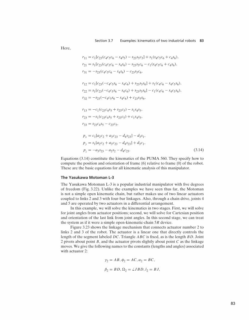
Section 3.7 Examples: kinematics of two industrial robots 83
Here,
r11 = c1[c23(c4c5c6 − s4s5) − s23s5c5] + s1(s4c5c6 + c4s6),
r21 = s1[c23(c4c5c6 − s4s6) − s23s5c6 − c1(s4c5c6 + c4s6),
r31 = −s23(c4c5c6 − s4s6) − c23s5c6,
r12 = c1[c23(−c4c5s6 − s4c6) + s23s5s6] + s1(c4c6 − s4c5s6),
r22 = s1[c23(−c4c5s6 − s4c6) + s23s5s6] − c1(c4c6 − s4c5s6),
r32 = −s23(−c4c5s6 − s4c6) + c23s5s6,
r13 = −c1(c23c4s5 + s23c5) − s1s4s5,
r23 = −s1(c23c4s5 + s23c5) + c1s4s5,
r33 = s23c4s5 − c23c5,
px = c1[a2c2 + a3c23 − d4s23] − d3s1,
py = s1[a2c2 + a3c23 − d4s23] + d3c1,
pz = −a3s23 − a2s2 − d4c23. (3.14)
Equations (3.14) constitute the kinematics of the PUMA 560. They specify how tocompute the position and orientation of frame {6} relative to frame {0} of the robot.These are the basic equations for all kinematic analysis of this manipulator.
The Yasukawa Motoman L-3
The Yasukawa Motoman L-3 is a popular industrial manipulator with five degreesof freedom (Fig. 3.22). Unlike the examples we have seen thus far, the Motomanis not a simple open kinematic chain, but rather makes use of two linear actuatorscoupled to links 2 and 3 with four-bar linkages. Also, through a chain drive, joints 4and 5 are operated by two actuators in a differential arrangement.
In this example, we will solve the kinematics in two stages. First, we will solvefor joint angles from actuator positions; second, we will solve for Cartesian positionand orientation of the last link from joint angles. In this second stage, we can treatthe system as if it were a simple open-kinematic-chain 5R device.
Figure 3.23 shows the linkage mechanism that connects actuator number 2 tolinks 2 and 3 of the robot. The actuator is a linear one that directly controls thelength of the segment labeled DC. Triangle ABC is fixed, as is the length BD. Joint2 pivots about point B, and the actuator pivots slightly about point C as the linkagemoves. We give the following names to the constants (lengths and angles) associatedwith actuator 2:
γ2 = AB, φ2 = AC, α2 = BC,
β2 = BD,,2 = JBD, l2 = BJ,
83
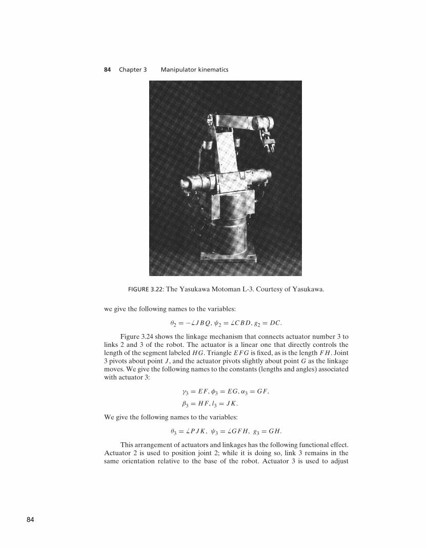
84 Chapter 3 Manipulator kinematics
FIGURE 3.22: The Yasukawa Motoman L-3. Courtesy of Yasukawa.
we give the following names to the variables:
θ2 = − JBQ,ψ2 = CBD, g2 = DC.
Figure 3.24 shows the linkage mechanism that connects actuator number 3 tolinks 2 and 3 of the robot. The actuator is a linear one that directly controls thelength of the segment labeled HG. Triangle EFG is fixed, as is the length FH . Joint3 pivots about point J , and the actuator pivots slightly about point G as the linkagemoves. We give the following names to the constants (lengths and angles) associatedwith actuator 3:
γ3 = EF, φ3 = EG, α3 = GF,
β3 = HF, l3 = JK.
We give the following names to the variables:
θ3 = PJK, ψ3 = GFH, g3 = GH.
This arrangement of actuators and linkages has the following functional effect.Actuator 2 is used to position joint 2; while it is doing so, link 3 remains in thesame orientation relative to the base of the robot. Actuator 3 is used to adjust
84
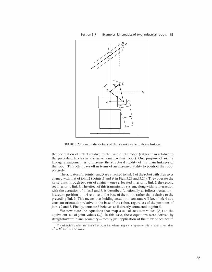
Section 3.7 Examples: kinematics of two industrial robots 85
A
B
C
D
Q
J
M
FIGURE 3.23: Kinematic details of the Yasukawa actuator-2 linkage.
the orientation of link 3 relative to the base of the robot (rather than relative tothe preceding link as in a serial-kinematic-chain robot). One purpose of such alinkage arrangement is to increase the structural rigidity of the main linkages ofthe robot. This often pays off in terms of an increased ability to position the robotprecisely.
The actuators for joints 4 and 5 are attached to link 1 of the robot with their axesaligned with that of joint 2 (points B and F in Figs. 3.23 and 3.24). They operate thewrist joints through two sets of chains—one set located interior to link 2, the secondset interior to link 3. The effect of this transmission system, along with its interactionwith the actuation of links 2 and 3, is described functionally as follows: Actuator 4is used to position joint 4 relative to the base of the robot, rather than relative to thepreceding link 3. This means that holding actuator 4 constant will keep link 4 at aconstant orientation relative to the base of the robot, regardless of the positions ofjoints 2 and 3. Finally, actuator 5 behaves as if directly connected to joint 5.
We now state the equations that map a set of actuator values (Ai) to theequivalent set of joint values (θi). In this case, these equations were derived bystraightforward plane geometry—mostly just application of the ‘‘law of cosines.’’7
7If a triangle’s angles are labeled a, b, and c, where angle a is opposite side A, and so on, then
A2 = B2 + C2 − 2BC cos a.
85
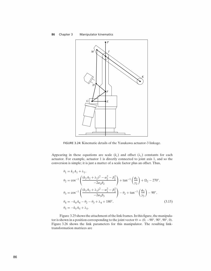
86 Chapter 3 Manipulator kinematics
EG
H
F
K
J
P
M
FIGURE 3.24: Kinematic details of the Yasukawa actuator-3 linkage.
Appearing in these equations are scale (ki) and offset (λi) constants for eachactuator. For example, actuator 1 is directly connected to joint axis 1, and so theconversion is simple; it is just a matter of a scale factor plus an offset. Thus,
θ1 = k1A1 + λ1,
θ2 = cos−1
(
(k2A2 + λ2)2 − α2
2− β2
2
−2α2β2
)
+ tan−1
(
φ2
γ2
)
+ ,2 − 270◦,
θ3 = cos−1
(
(k3A3 + λ3)2 − α2
3− β2
3
−2α3β3
)
− θ2 + tan−1
(
φ3
γ3
)
− 90◦,
θ4 = −k4A4 − θ2 − θ3 + λ4 + 180◦, (3.15)
θ5 = −k5A5 + λ5.
Figure 3.25 shows the attachment of the link frames. In this figure, the manipula-tor is shown in a position corresponding to the joint vector 6 = (0,−90◦, 90◦, 90◦, 0).Figure 3.26 shows the link parameters for this manipulator. The resulting link-transformation matrices are
86
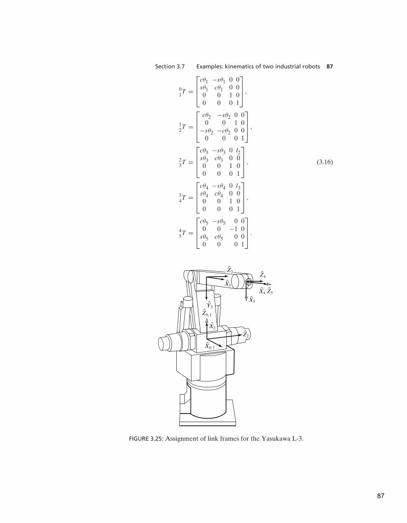
Section 3.7 Examples: kinematics of two industrial robots 87
01T =
cθ1 −sθ1 0 0sθ1 cθ1 0 00 0 1 00 0 0 1
,
12T =
cθ2 −sθ2 0 00 0 1 0
−sθ2 −cθ2 0 00 0 0 1
,
23T =
cθ3 −sθ3 0 l2sθ3 cθ3 0 00 0 1 00 0 0 1
, (3.16)
34T =
cθ4 −sθ4 0 l3sθ4 cθ4 0 00 0 1 00 0 0 1
,
45T =
cθ5 −sθ5 0 00 0 −1 0
sθ5 cθ5 0 00 0 0 1
.
X5
Z5
Z4
Z2
Z3
Y3
X2
Z0, 1
X0, 1
X4
X3
FIGURE 3.25: Assignment of link frames for the Yasukawa L-3.
87
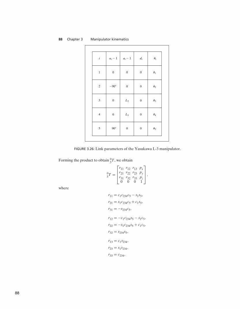
88 Chapter 3 Manipulator kinematics
5
4
3
2
1
i
0
0
0
ai � 1
0
L3
L2
0
0
ai � 1
0
0
0
0
0
di
u5
u4
u3
u2
u1
ui
�90
90
FIGURE 3.26: Link parameters of the Yasukawa L-3 manipulator.
Forming the product to obtain 05T , we obtain
05T =
r11 r12 r13 px
r21 r22 r23 py
r31 r32 r33 pz
0 0 0 1
,
where
r11 = c1c234c5 − s1s5,
r21 = s1c234c5 + c1s5,
r31 = −s234c5,
r12 = −c1c234s5 − s1c5,
r22 = −s1c234s5 + c1c5,
r32 = s234s5,
r13 = c1s234,
r23 = s1s234,
r33 = c234,
88
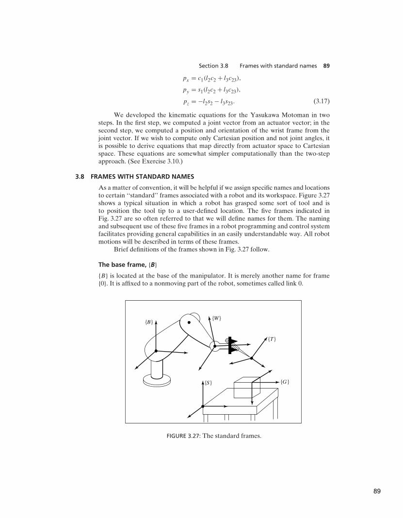
Section 3.8 Frames with standard names 89
px = c1(l2c2 + l3c23),
py = s1(l2c2 + l3c23),
pz = −l2s2 − l3s23. (3.17)
We developed the kinematic equations for the Yasukawa Motoman in twosteps. In the first step, we computed a joint vector from an actuator vector; in thesecond step, we computed a position and orientation of the wrist frame from thejoint vector. If we wish to compute only Cartesian position and not joint angles, itis possible to derive equations that map directly from actuator space to Cartesianspace. These equations are somewhat simpler computationally than the two-stepapproach. (See Exercise 3.10.)
3.8 FRAMES WITH STANDARD NAMES
As a matter of convention, it will be helpful if we assign specific names and locationsto certain ‘‘standard’’ frames associated with a robot and its workspace. Figure 3.27shows a typical situation in which a robot has grasped some sort of tool and isto position the tool tip to a user-defined location. The five frames indicated inFig. 3.27 are so often referred to that we will define names for them. The namingand subsequent use of these five frames in a robot programming and control systemfacilitates providing general capabilities in an easily understandable way. All robotmotions will be described in terms of these frames.
Brief definitions of the frames shown in Fig. 3.27 follow.
The base frame, {B}
{B} is located at the base of the manipulator. It is merely another name for frame{0}. It is affixed to a nonmoving part of the robot, sometimes called link 0.
�B ��W �
�S � �G �
�T �
FIGURE 3.27: The standard frames.
89

90 Chapter 3 Manipulator kinematics
The station frame, {S}
{S} is located in a task-relevant location. In Fig. 3.28, it is at the corner of a tableupon which the robot is to work. As far as the user of this robot system is concerned,{S} is the universe frame, and all actions of the robot are performed relative to it.It is sometimes called the task frame, the world frame, or the universe frame. Thestation frame is always specified with respect to the base frame, that is, B
ST .
The wrist frame, {W}
{W } is affixed to the last link of the manipulator. It is another name for frame {N}, thelink frame attached to the last link of the robot. Very often, {W } has its origin fixedat a point called the wrist of the manipulator, and {W } moves with the last link ofthe manipulator. It is defined relative to the base frame—that is, {W } = B
WT = 0
NT .
The tool frame, {T}
{T } is affixed to the end of any tool the robot happens to be holding. When thehand is empty, {T } is usually located with its origin between the fingertips ofthe robot. The tool frame is always specified with respect to the wrist frame. InFig. 3.28, the tool frame is defined with its origin at the tip of a pin that the robot isholding.
Goalframe
Stationframe
Base frame
Wrist frame
Tool frame
Pin
Camera
FIGURE 3.28: Example of the assignment of standard frames.
90

Section 3.9 Where is the tool? 91
The goal frame, {G}
{G} is a description of the location to which the robot is to move the tool. Specificallythis means that, at the end of the motion, the tool frame should be brought tocoincidence with the goal frame. {G} is always specified relative to the station frame.In Fig. 3.28, the goal is located at a hole into which we want the pin to be inserted.
All robot motions may be described in terms of these frames without lossof generality. Their use helps to give us a standard language for talking aboutrobot tasks.
3.9 WHERE IS THE TOOL?
One of the first capabilities a robot must have is to be able to calculate the positionand orientation of the tool it is holding (or of its empty hand) with respect to aconvenient coordinate system. That is, we wish to calculate the value of the toolframe, {T }, relative to the station frame, {S}. Once B
WT has been computed via the
kinematic equations, we can use Cartesian transforms, as studied in Chapter 2, tocalculate {T } relative to {S}. Solving a simple transform equation leads to
S
TT = B
ST −1 B
WT W
TT . (3.18)
Equation (3.18) implements what is called the WHERE function in some robotsystems. It computes ‘‘where’’ the arm is. For the situation in Fig. 3.28, the output ofWHERE would be the position and orientation of the pin relative to the table top.
Equation (3.18) can be thought of as generalizing the kinematics. STT computes
the kinematics due to the geometry of the linkages, along with a general transform(which might be considered a fixed link) at the base end (B
ST ) and another at the
end-effector (WT
T ). These extra transforms allow us to include tools with offsets andtwists and to operate with respect to an arbitrary station frame.
3.10 COMPUTATIONAL CONSIDERATIONS
In many practical manipulator systems, the time required to perform kinematiccalculations is a consideration. In this section, we briefly discuss various issuesinvolved in computing manipulator kinematics, as exemplified by (3.14), for the caseof the PUMA 560.
One choice to be made is the use of fixed- or floating-point representationof the quantities involved. Many implementations use floating point for ease ofsoftware development, because the programmer does not have to be concernedwith scaling operations capturing the relative magnitudes of the variables. However,when speed is crucial, fixed-point representation is quite possible, because thevariables do not have a large dynamic range, and these ranges are fairly well known.Rough estimations of the number of bits needed in fixed-point representation seemto indicate that 24 are sufficient [4].
By factoring equations such as (3.14), it is possible to reduce the number ofmultiplications and additions—at the cost of creating local variables (usually a goodtrade-off). The point is to avoid computing common terms over and over throughoutthe computation. There has been some application of computer-assisted automaticfactorization of such equations [5].
91

92 Chapter 3 Manipulator kinematics
The major expense in calculating kinematics is often the calculation of thetranscendental functions (sine and cosine). When these functions are available aspart of a standard library, they are often computed from a series expansion atthe cost of many multiply times. At the expense of some required memory, manymanipulation systems employ table-lookup implementations of the transcendentalfunctions. Depending on the scheme, this reduces the amount of time required tocalculate a sine or cosine to two or three multiply times or less [6].
The computation of the kinematics as in (3.14) is redundant, in that ninequantities are calculated to represent orientation. One means that usually reducescomputation is to calculate only two columns of the rotation matrix and then tocompute a cross product (requiring only six multiplications and three additions)to compute the third column. Obviously, one chooses the two least complicatedcolumns to compute.
BIBLIOGRAPHY
[1] J. Denavit and R.S. Hartenberg, ‘‘A Kinematic Notation for Lower-Pair MechanismsBased on Matrices,’’ Journal of Applied Mechanics, pp. 215–221, June 1955.
[2] J. Lenarcic, ‘‘Kinematics,’’ in The International Encyclopedia of Robotics, R. Dorf andS. Nof, Editors, John C. Wiley and Sons, New York, 1988.
[3] J. Colson and N.D. Perreira, ‘‘Kinematic Arrangements Used in Industrial Robots,’’13th Industrial Robots Conference Proceedings, April 1983.
[4] T. Turner, J. Craig, and W. Gruver, ‘‘A Microprocessor Architecture for AdvancedRobot Control,’’ 14th ISIR, Stockholm, Sweden, October 1984.
[5] W. Schiehlen, ‘‘Computer Generation of Equations of Motion,’’ in Computer Aided
Analysis and Optimization of Mechanical System Dynamics, E.J. Haug, Editor, Springer-Verlag, Berlin & New York, 1984.
[6] C. Ruoff, ‘‘Fast Trigonometric Functions for Robot Control,’’ Robotics Age, November1981.
EXERCISES
3.1 [15] Compute the kinematics of the planar arm from Example 3.3.3.2 [37] Imagine an arm like the PUMA 560, except that joint 3 is replaced with
a prismatic joint. Assume the prismatic joint slides along the direction of X1 inFig. 3.18; however, there is still an offset equivalent to d3 to be accounted for.Make any additional assumptions needed. Derive the kinematic equations.
3.3 [25] The arm with three degrees of freedom shown in Fig. 3.29 is like the one inExample 3.3, except that joint 1’s axis is not parallel to the other two. Instead,there is a twist of 90 degrees in magnitude between axes 1 and 2. Derive linkparameters and the kinematic equations for B
WT . Note that no l3 need be defined.
3.4 [22] The arm with three degrees of freedom shown in Fig. 3.30 has joints 1and 2 perpendicular and joints 2 and 3 parallel. As pictured, all joints are attheir zero location. Note that the positive sense of the joint angle is indicated.Assign link frames {0} through {3} for this arm—that is, sketch the arm, showingthe attachment of the frames. Then derive the transformation matrices 0
1T , 1
2T ,
and 23T .
92

Exercises 93
L1
L2
u1u2
u3
FIGURE 3.29: The 3R nonplanar arm (Exercise 3.3).
L1
L2
L3 L4
XT
XS
YS
ZT
ZS
YT �T �
u1
u3
u2
FIGURE 3.30: Two views of a 3R manipulator (Exercise 3.4).
3.5 [26] Write a subroutine to compute the kinematics of a PUMA 560. Code forspeed, trying to minimize the number of multiplications as much as possible. Usethe procedure heading (or equivalent in C)
Procedure KIN(VAR theta: vec6; VAR wrelb: frame);
Count a sine or cosine evaluation as costing 5 multiply times. Count additionsas costing 0.333 multiply times and assignment statements as 0.2 multiply times.
93

94 Chapter 3 Manipulator kinematics
Count a square-root computation as costing 4 multiply times. How many multiplytimes do you need?
3.6 [20] Write a subroutine to compute the kinematics of the cylindrical arm inExample 3.4. Use the procedure heading (or equivalent in C)
Procedure KIN(VAR jointvar: vec3; VAR wrelb: frames);
Count a sine or cosine evaluation as costing 5 multiply times. Count additionsas costing 0.333 multiply times and assignment statements as 0.2 multiply times.Count a square-root computation as costing 4 multiply times. How many multiplytimes do you need?
3.7 [22] Write a subroutine to compute the kinematics of the arm in Exercise 3.3. Usethe procedure heading (or equivalent in C)
Procedure KIN(VAR theta: vec3; VAR wrelb: frame);
Count a sine or cosine evaluation as costing 5 multiply times. Count additionsas costing 0.333 multiply times and assignment statements as 0.2 multiply times.Count a square-root computation as costing 4 multiply times. How many multiplytimes do you need?
3.8 [13] In Fig. 3.31, the location of the tool, WT
T , is not accurately known. Using forcecontrol, the robot feels around with the tool tip until it inserts it into the socket(or Goal) at location S
GT . Once in this ‘‘calibration’’ configuration (in which {G}
and {T } are coincident), the position of the robot, BW
T , is figured out by reading
the joint angle sensors and computing the kinematics. Assuming BST and S
GT are
known, give the transform equation to compute the unknown tool frame, WT
T .
ZG
YG
XG
ZT
XT
YT
�S �
�G �
�W ��B � �T �
FIGURE 3.31: Determination of the tool frame (Exercise 3.8).
94

Exercises 95
(a) (b)
Tip
L1
L2
Y2
X1, 0
Z1, 0X2
FIGURE 3.32: Two-link arm with frame assignments (Exercise 3.9).
3.9 [11] For the two-link manipulator shown in Fig. 3.32(a), the link-transformationmatrices, 0
1T and 1
2T , were constructed. Their product is
02T =
cθ1cθ2 −cθ1sθ2 sθ1 l1cθ1sθ1cθ2 −sθ1sθ2 −cθ1 l1sθ1sθ2 cθ2 0 00 0 0 1
.
The link-frame assignments used are indicated in Fig. 3.32(b). Note that frame{0} is coincident with frame {1} when θ1 = 0. The length of the second link is l2.Find an expression for the vector 0Pt ip , which locates the tip of the arm relativeto the {0} frame.
3.10 [39] Derive kinematic equations for the Yasukawa Motoman robot (seeSection 3.7) that compute the position and orientation of the wrist frame directlyfrom actuator values, rather than by first computing the joint angles. A solutionis possible that requires only 33 multiplications, two square roots, and six sine orcosine evaluations.
3.11 [17] Figure 3.33 shows the schematic of a wrist which has three intersecting axesthat are not orthogonal. Assign link frames to this wrist (as if it were a 3-DOFmanipulator), and give the link parameters.
3.12 [08] Can an arbitrary rigid-body transformation always be expressed with fourparameters (a, α, d , θ) in the form of equation (3.6)?
3.13 [15] Show the attachment of link frames for the 5-DOF manipulator shownschematically in Fig. 3.34.
3.14 [20] As was stated, the relative position of any two lines in space can be givenwith two parameters, a and α, where a is the length of the common perpendicularjoining the two and α is the angle made by the two axes when projected ontoa plane normal to the common perpendicular. Given a line defined as passingthrough point p with unit-vector direction m and a second passing through pointq with unit-vector direction n, write expressions for a and α.
3.15 [15] Show the attachment of link frames for the 3-DOF manipulator shownschematically in Fig. 3.35.
3.16 [15] Assign link frames to the RPR planar robot shown in Fig. 3.36, and give thelinkage parameters.
3.17 [15] Show the attachment of link frames on the three-link robot shown in Fig. 3.37.
95

96 Chapter 3 Manipulator kinematics
u6
u5
u4
f
FIGURE 3.33: 3R nonorthogonal-axis robot (Exercise 3.11).
u1
u2
u4
d3 u5
FIGURE 3.34: Schematic of a 2RP 2R manipulator (Exercise 3.13).
3.18 [15] Show the attachment of link frames on the three-link robot shown in Fig. 3.38.3.19 [15] Show the attachment of link frames on the three-link robot shown in Fig. 3.39.3.20 [15] Show the attachment of link frames on the three-link robot shown in Fig. 3.40.3.21 [15] Show the attachment of link frames on the three-link robot shown in Fig. 3.41.3.22 [18] Show the attachment of link frames on the P 3R robot shown in Fig. 3.42.
Given your frame assignments, what are the signs of d2, d3, and a2?
96
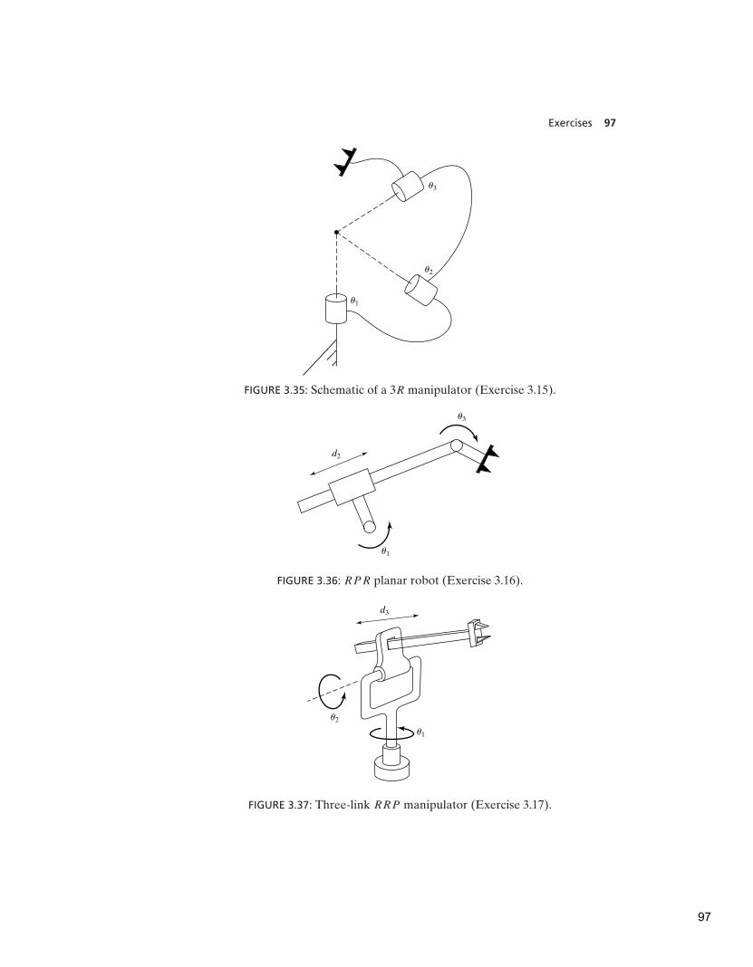
Exercises 97
u1
u3
u2
FIGURE 3.35: Schematic of a 3R manipulator (Exercise 3.15).
u3
d2
u1
FIGURE 3.36: RPR planar robot (Exercise 3.16).
u1
u2
d3
FIGURE 3.37: Three-link RRP manipulator (Exercise 3.17).
97
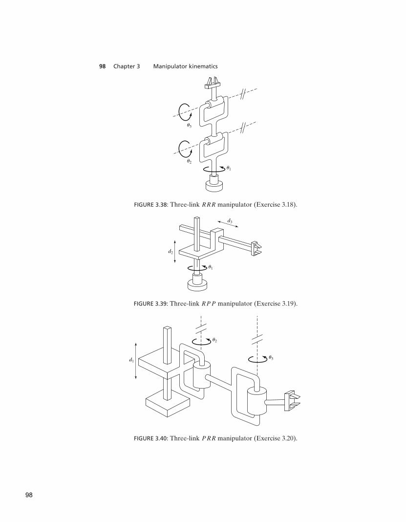
98 Chapter 3 Manipulator kinematics
u1
u2
u3
FIGURE 3.38: Three-link RRR manipulator (Exercise 3.18).
u1
d3
d2
FIGURE 3.39: Three-link RPP manipulator (Exercise 3.19).
u2
d1u3
FIGURE 3.40: Three-link PRR manipulator (Exercise 3.20).
98

Programming exercise (Part 3) 99
d1
d2
d3
FIGURE 3.41: Three-link PPP manipulator (Exercise 3.21).
FIGURE 3.42: Schematic of a P 3R manipulator (Exercise 3.22).
PROGRAMMING EXERCISE (PART 3)
1. Write a subroutine to compute the kinematics of the planar 3R robot in Exam-ple 3.3—that is, a routine with the joint angles’ values as input, and a frame (thewrist frame relative to the base frame) as output. Use the procedure heading (orequivalent in C)
Procedure KIN(VAR theta: vec3; VAR wrelb: frame);
where ‘‘wrelb’’ is the wrist frame relative to the base frame, BW
T . The type ‘‘frame’’consists of a 2 × 2 rotation matrix and a 2 × 1 position vector. If desired, you mayrepresent the frame with a 3 × 3 homogeneous transform in which the third row is[0 0 1]. (The manipulator data are l1 = l2 = 0.5 meters.)
99

100 Chapter 3 Manipulator kinematics
2. Write a routine that calculates where the tool is, relative to the station frame. Theinput to the routine is a vector of joint angles:
Procedure WHERE(VAR theta: vec3; VAR trels: frame);
Obviously, WHERE must make use of descriptions of the tool frame and therobot base frame in order to compute the location of the tool relative to the stationframe. The values of W
TT and S
BT should be stored in global memory (or, as a
second choice, you may pass them as arguments in WHERE).
3. A tool frame and a station frame for a certain task are defined as follows by theuser:
W
TT = [x y θ] = [0.1 0.2 30.0],
B
ST = [x y θ] = [−0.1 0.3 0.0].
Calculate the position and orientation of the tool relative to the station frame forthe following three configurations (in units of degrees) of the arm:
[θ1 θ2 θ3] = [0.0 90.0 − 90.0],
[θ1 θ2 θ3] = [−23.6 − 30.3 48.0],
[θ1 θ2 θ3] = [130.0 40.0 12.0].
MATLAB EXERCISE 3
This exercise focuses on DH parameters and on the forward-pose (position and orien-tation) kinematics transformation for the planar 3-DOF, 3R robot (of Figures 3.6 and3.7). The following fixed-length parameters are given: L1 = 4, L2 = 3, and L3 = 2 (m).
a) Derive the DH parameters. You can check your results against Figure 3.8.
b) Derive the neighboring homogeneous transformation matrices i−1iT , i = 1, 2, 3.
These are functions of the joint-angle variables θi , i = 1, 2, 3. Also, derive theconstant 3
HT by inspection: The origin of {H } is in the center of the gripper fingers,
and the orientation of {H } is always the same as the orientation of {3}.
c) Use Symbolic MATLAB to derive the forward-pose kinematics solution 03T and
0HT symbolically (as a function of θ i). Abbreviate your answer, using si = sin(θi),
ci = cos(θi), and so on. Also, there is a (θ1 + θ2 + θ3) simplification, by using sum-of-angle formulas, that is due to the parallel Zi axes. Calculate the forward-posekinematics results (both 0
3T and 0
HT ) via MATLAB for the following input cases:
i) 6 = {θ1 θ2 θ3}T = {0 0 0}T .
ii) 6 = {10◦
20◦
30◦}T .
iii) 6 = {90◦
90◦
90◦}T .
For all three cases, check your results by sketching the manipulator configurationand deriving the forward-pose kinematics transformation by inspection. (Think ofthe definition of 0
HT in terms of a rotation matrix and a position vector.) Include
frames {H }, {3}, and {0} in your sketches.
d) Check all your results by means of the Corke MATLAB Robotics Toolbox. Tryfunctions link(), robot(), and fkine().
100
C H A P T E R 4
Inverse manipulator kinematics
4.1 INTRODUCTION
4.2 SOLVABILITY
4.3 THE NOTION OF MANIPULATOR SUBSPACE WHEN n < 6
4.4 ALGEBRAIC VS. GEOMETRIC
4.5 ALGEBRAIC SOLUTION BY REDUCTION TO POLYNOMIAL
4.6 PIEPER’S SOLUTION WHEN THREE AXES INTERSECT
4.7 EXAMPLES OF INVERSE MANIPULATOR KINEMATICS
4.8 THE STANDARD FRAMES
4.9 SOLVE-ING A MANIPULATOR
4.10 REPEATABILITY AND ACCURACY
4.11 COMPUTATIONAL CONSIDERATIONS
4.1 INTRODUCTION
In the last chapter, we considered the problem of computing the position andorientation of the tool relative to the user’s workstation when given the joint anglesof the manipulator. In this chapter, we investigate the more difficult converseproblem: Given the desired position and orientation of the tool relative to thestation, how do we compute the set of joint angles which will achieve this desiredresult? Whereas Chapter 3 focused on the direct kinematics of manipulators, herethe focus is the inverse kinematics of manipulators.
Solving the problem of finding the required joint angles to place the toolframe, {T }, relative to the station frame, {S}, is split into two parts. First, frametransformations are performed to find the wrist frame, {W }, relative to the baseframe, {B}, and then the inverse kinematics are used to solve for the joint angles.
4.2 SOLVABILITY
The problem of solving the kinematic equations of a manipulator is a nonlinear one.Given the numerical value of 0
NT , we attempt to find values of θ1, θ2, . . ., θn. Consider
the equations given in (3.14). In the case of the PUMA 560 manipulator, the precisestatement of our current problem is as follows: Given 0
6T as sixteen numeric values
(four of which are trivial), solve (3.14) for the six joint angles θ1 through θ6.For the case of an arm with six degrees of freedom (like the one corresponding
to the equations in (3.14)), we have 12 equations and six unknowns. However,among the 9 equations arising from the rotation-matrix portion of 0
6T , only 3 are
independent. These, added to the 3 equations from the position-vector portion of 06T ,
From Chapter 4 of Introduction to Robotics: Mechanics and Control, Third Edition. John J. Craig.
Copyright © 2005 by Pearson Education, Inc. All rights reserved.
101
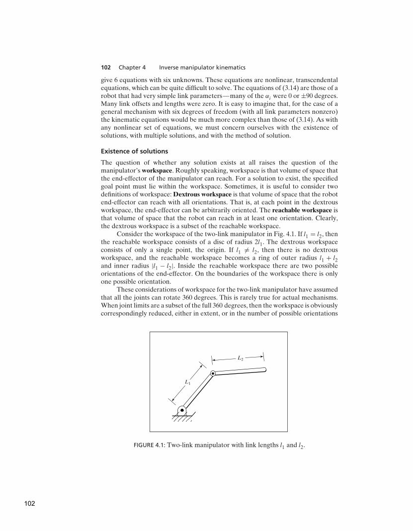
102 Chapter 4 Inverse manipulator kinematics
give 6 equations with six unknowns. These equations are nonlinear, transcendentalequations, which can be quite difficult to solve. The equations of (3.14) are those of arobot that had very simple link parameters—many of the αi were 0 or ±90 degrees.Many link offsets and lengths were zero. It is easy to imagine that, for the case of ageneral mechanism with six degrees of freedom (with all link parameters nonzero)the kinematic equations would be much more complex than those of (3.14). As withany nonlinear set of equations, we must concern ourselves with the existence ofsolutions, with multiple solutions, and with the method of solution.
Existence of solutions
The question of whether any solution exists at all raises the question of themanipulator’s workspace. Roughly speaking, workspace is that volume of space thatthe end-effector of the manipulator can reach. For a solution to exist, the specifiedgoal point must lie within the workspace. Sometimes, it is useful to consider twodefinitions of workspace: Dextrous workspace is that volume of space that the robotend-effector can reach with all orientations. That is, at each point in the dextrousworkspace, the end-effector can be arbitrarily oriented. The reachable workspace isthat volume of space that the robot can reach in at least one orientation. Clearly,the dextrous workspace is a subset of the reachable workspace.
Consider the workspace of the two-link manipulator in Fig. 4.1. If l1 = l2, thenthe reachable workspace consists of a disc of radius 2l1. The dextrous workspaceconsists of only a single point, the origin. If l1 �= l2, then there is no dextrousworkspace, and the reachable workspace becomes a ring of outer radius l1 + l2and inner radius |l1 − l2|. Inside the reachable workspace there are two possibleorientations of the end-effector. On the boundaries of the workspace there is onlyone possible orientation.
These considerations of workspace for the two-link manipulator have assumedthat all the joints can rotate 360 degrees. This is rarely true for actual mechanisms.When joint limits are a subset of the full 360 degrees, then the workspace is obviouslycorrespondingly reduced, either in extent, or in the number of possible orientations
L2
L1
FIGURE 4.1: Two-link manipulator with link lengths l1 and l2.
102
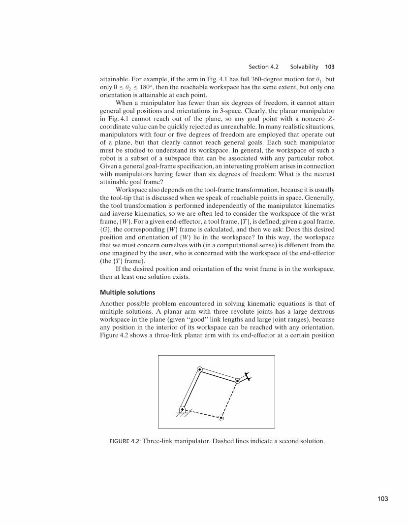
Section 4.2 Solvability 103
attainable. For example, if the arm in Fig. 4.1 has full 360-degree motion for θ1, butonly 0 ≤ θ2 ≤ 180◦, then the reachable workspace has the same extent, but only oneorientation is attainable at each point.
When a manipulator has fewer than six degrees of freedom, it cannot attaingeneral goal positions and orientations in 3-space. Clearly, the planar manipulatorin Fig. 4.1 cannot reach out of the plane, so any goal point with a nonzero Z-coordinate value can be quickly rejected as unreachable. In many realistic situations,manipulators with four or five degrees of freedom are employed that operate outof a plane, but that clearly cannot reach general goals. Each such manipulatormust be studied to understand its workspace. In general, the workspace of such arobot is a subset of a subspace that can be associated with any particular robot.Given a general goal-frame specification, an interesting problem arises in connectionwith manipulators having fewer than six degrees of freedom: What is the nearestattainable goal frame?
Workspace also depends on the tool-frame transformation, because it is usuallythe tool-tip that is discussed when we speak of reachable points in space. Generally,the tool transformation is performed independently of the manipulator kinematicsand inverse kinematics, so we are often led to consider the workspace of the wristframe, {W }. For a given end-effector, a tool frame, {T }, is defined; given a goal frame,{G}, the corresponding {W } frame is calculated, and then we ask: Does this desiredposition and orientation of {W } lie in the workspace? In this way, the workspacethat we must concern ourselves with (in a computational sense) is different from theone imagined by the user, who is concerned with the workspace of the end-effector(the {T } frame).
If the desired position and orientation of the wrist frame is in the workspace,then at least one solution exists.
Multiple solutions
Another possible problem encountered in solving kinematic equations is that ofmultiple solutions. A planar arm with three revolute joints has a large dextrousworkspace in the plane (given ‘‘good’’ link lengths and large joint ranges), becauseany position in the interior of its workspace can be reached with any orientation.Figure 4.2 shows a three-link planar arm with its end-effector at a certain position
FIGURE 4.2: Three-link manipulator. Dashed lines indicate a second solution.
103

104 Chapter 4 Inverse manipulator kinematics
Obstacle
A
B
FIGURE 4.3: One of the two possible solutions to reach point B causes a collision.
and orientation. The dashed lines indicate a second possible configuration in whichthe same end-effector position and orientation are achieved.
The fact that a manipulator has multiple solutions can cause problems, becausethe system has to be able to choose one. The criteria upon which to base a decisionvary, but a very reasonable choice would be the closest solution. For example, if themanipulator is at point A, as in Fig. 4.3, and we wish to move it to point B, a goodchoice would be the solution that minimizes the amount that each joint is requiredto move. Hence, in the absence of the obstacle, the upper dashed configuration inFig. 4.3 would be chosen. This suggests that one input argument to our kinematicinverse procedure might be the present position of the manipulator. In this way,if there is a choice, our algorithm can choose the solution closest in joint-space.However, the notion of ‘‘close’’ might be defined in several ways. For example,typical robots could have three large links followed by three smaller, orienting linksnear the end-effector. In this case, weights might be applied in the calculation ofwhich solution is ‘‘closer’’ so that the selection favors moving smaller joints ratherthan moving the large joints, when a choice exists. The presence of obstacles mightforce a ‘‘farther’’ solution to be chosen in cases where the ‘‘closer’’ solution wouldcause a collision—in general, then, we need to be able to calculate all the possiblesolutions. Thus, in Fig. 4.3, the presence of the obstacle implies that the lower dashedconfiguration is to be used to reach point B.
The number of solutions depends upon the number of joints in the manipulatorbut is also a function of the link parameters (αi , ai , and di for a rotary jointmanipulator) and the allowable ranges of motion of the joints. For example, thePUMA 560 can reach certain goals with eight different solutions. Figure 4.4 showsfour solutions; all place the hand with the same position and orientation. For eachsolution pictured, there is another solution in which the last three joints ‘‘flip’’ to analternate configuration according to the following formulas:
θ ′4
= θ4 + 180◦,
θ ′5
= −θ5, (4.1)
θ ′6
= θ6 + 180◦.
So, in total, there can be eight solutions for a single goal. Because of limits on jointranges, some of these eight could be inaccessible.
104

Section 4.2 Solvability 105
FIGURE 4.4: Four solutions of the PUMA 560.
In general, the more nonzero link parameters there are, the more ways therewill be to reach a certain goal. For example, consider a manipulator with sixrotational joints. Figure 4.5 shows how the maximum number of solutions is relatedto how many of the link length parameters (the ai) are zero. The more that arenonzero, the bigger is the maximum number of solutions. For a completely generalrotary-jointed manipulator with six degrees of freedom, there are up to sixteensolutions possible [1, 6].
Method of solution
Unlike linear equations, there are no general algorithms that may be employed tosolve a set of nonlinear equations. In considering methods of solution, it will be wiseto define what constitutes the ‘‘solution’’ of a given manipulator.
A manipulator will be considered solvable if the joint variables can bedetermined by an algorithm that allows one to determine all the sets of jointvariables associated with a given position and orientation [2].
105
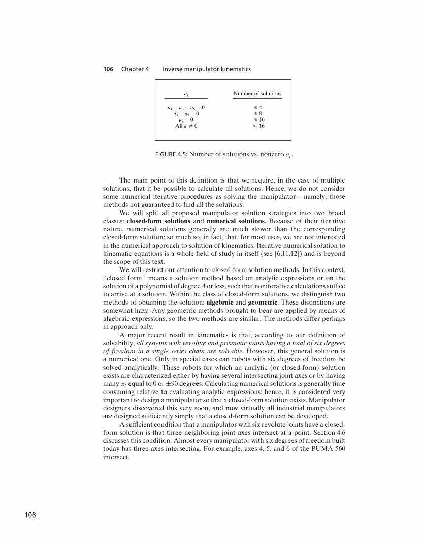
106 Chapter 4 Inverse manipulator kinematics
ai
a1 � a3 � a5 � 0a3 � a5 � 0
a3 � 0All ai � 0
Number of solutions
� 4� 8
� 16 � 16
FIGURE 4.5: Number of solutions vs. nonzero ai .
The main point of this definition is that we require, in the case of multiplesolutions, that it be possible to calculate all solutions. Hence, we do not considersome numerical iterative procedures as solving the manipulator—namely, thosemethods not guaranteed to find all the solutions.
We will split all proposed manipulator solution strategies into two broadclasses: closed-form solutions and numerical solutions. Because of their iterativenature, numerical solutions generally are much slower than the correspondingclosed-form solution; so much so, in fact, that, for most uses, we are not interestedin the numerical approach to solution of kinematics. Iterative numerical solution tokinematic equations is a whole field of study in itself (see [6,11,12]) and is beyondthe scope of this text.
We will restrict our attention to closed-form solution methods. In this context,‘‘closed form’’ means a solution method based on analytic expressions or on thesolution of a polynomial of degree 4 or less, such that noniterative calculations sufficeto arrive at a solution. Within the class of closed-form solutions, we distinguish twomethods of obtaining the solution: algebraic and geometric. These distinctions aresomewhat hazy: Any geometric methods brought to bear are applied by means ofalgebraic expressions, so the two methods are similar. The methods differ perhapsin approach only.
A major recent result in kinematics is that, according to our definition ofsolvability, all systems with revolute and prismatic joints having a total of six degrees
of freedom in a single series chain are solvable. However, this general solution isa numerical one. Only in special cases can robots with six degrees of freedom besolved analytically. These robots for which an analytic (or closed-form) solutionexists are characterized either by having several intersecting joint axes or by havingmany αi equal to 0 or ±90 degrees. Calculating numerical solutions is generally timeconsuming relative to evaluating analytic expressions; hence, it is considered veryimportant to design a manipulator so that a closed-form solution exists. Manipulatordesigners discovered this very soon, and now virtually all industrial manipulatorsare designed sufficiently simply that a closed-form solution can be developed.
A sufficient condition that a manipulator with six revolute joints have a closed-form solution is that three neighboring joint axes intersect at a point. Section 4.6discusses this condition. Almost every manipulator with six degrees of freedom builttoday has three axes intersecting. For example, axes 4, 5, and 6 of the PUMA 560intersect.
106
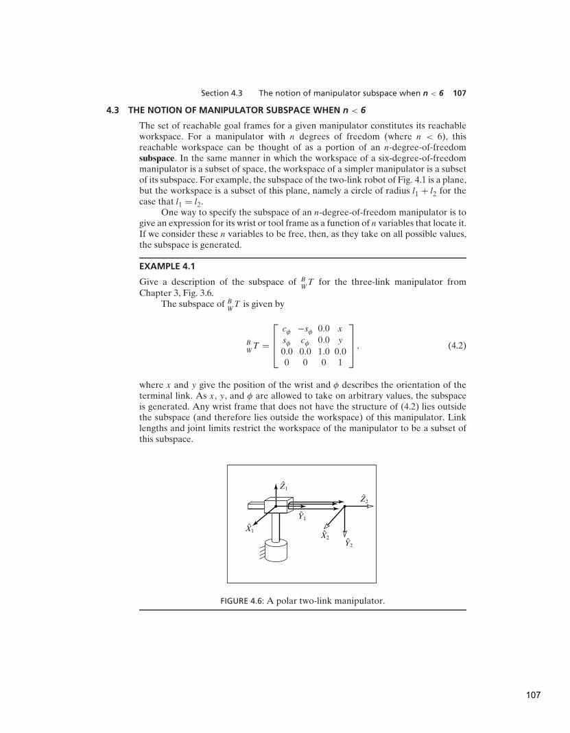
Section 4.3 The notion of manipulator subspace when n < 6 107
4.3 THE NOTION OF MANIPULATOR SUBSPACE WHEN n < 6
The set of reachable goal frames for a given manipulator constitutes its reachableworkspace. For a manipulator with n degrees of freedom (where n < 6), thisreachable workspace can be thought of as a portion of an n-degree-of-freedomsubspace. In the same manner in which the workspace of a six-degree-of-freedommanipulator is a subset of space, the workspace of a simpler manipulator is a subsetof its subspace. For example, the subspace of the two-link robot of Fig. 4.1 is a plane,but the workspace is a subset of this plane, namely a circle of radius l1 + l2 for thecase that l1 = l2.
One way to specify the subspace of an n-degree-of-freedom manipulator is togive an expression for its wrist or tool frame as a function of n variables that locate it.If we consider these n variables to be free, then, as they take on all possible values,the subspace is generated.
EXAMPLE 4.1
Give a description of the subspace of BW
T for the three-link manipulator fromChapter 3, Fig. 3.6.
The subspace of BW
T is given by
B
WT =
cφ −sφ 0.0 x
sφ cφ 0.0 y
0.0 0.0 1.0 0.00 0 0 1
, (4.2)
where x and y give the position of the wrist and φ describes the orientation of theterminal link. As x, y, and φ are allowed to take on arbitrary values, the subspaceis generated. Any wrist frame that does not have the structure of (4.2) lies outsidethe subspace (and therefore lies outside the workspace) of this manipulator. Linklengths and joint limits restrict the workspace of the manipulator to be a subset ofthis subspace.
X2
X1
Y2
Y1
Z2
Z1
FIGURE 4.6: A polar two-link manipulator.
107

108 Chapter 4 Inverse manipulator kinematics
EXAMPLE 4.2
Give a description of the subspace of 02T for the polar manipulator with two degrees
of freedom shown in Fig. 4.6. We have
0P2ORG =
x
y
0
, (4.3)
where x and y can take any values. The orientation is restricted because the 0Z2 axis
must point in a direction that depends on x and y. The 0Y2 axis always points down,
and the 0X2 axis can be computed as the cross product 0Y2 × 0Z2. In terms of x andy, we have
0Z2 =
x√
x2 + y2
y√
x2 + y2
0
. (4.4)
The subspace can therefore be given as
02T =
y√
x2 + y20
x√
x2 + y2x
−x√
x2 + y20
y√
x2 + y2y
0 −1 0 00 0 0 1
. (4.5)
Usually, in defining a goal for a manipulator with n degrees of freedom, weuse n parameters to specify the goal. If, on the other hand, we give a specification ofa full six degrees of freedom, we will not in general be able to reach the goal withan n < 6 manipulator. In this case, we might be interested instead in reaching a goalthat lies in the manipulator’s subspace and is as ‘‘near’’ as possible to the originaldesired goal.
Hence, when specifying general goals for a manipulator with fewer than sixdegrees of freedom, one solution strategy is the following:
1. Given a general goal frame, SGT , compute a modified goal frame, S
G′T , such
that SG′T lies in the manipulator’s subspace and is as ‘‘near’’ to S
GT as possible.
A definition of ‘‘near’’ must be chosen.
2. Compute the inverse kinematics to find joint angles using SG′T as the desired
goal. Note that a solution still might not be possible if the goal point is not inthe manipulator’s workspace.
It generally makes sense to position the tool-frame origin to the desired locationand then choose an attainable orientation that is near the desired orientation. Aswe saw in Examples 4.1 and 4.2, computation of the subspace is dependent onmanipulator geometry. Each manipulator must be individually considered to arriveat a method of making this computation.
108

Section 4.4 Algebraic vs. geometric 109
Section 4.7 gives an example of projecting a general goal into the subspace of amanipulator with five degrees of freedom in order to compute joint angles that willresult in the manipulator’s reaching the attainable frame nearest to the desired one.
4.4 ALGEBRAIC VS. GEOMETRIC
As an introduction to solving kinematic equations, we will consider two differentapproaches to the solution of a simple planar three-link manipulator.
Algebraic solution
Consider the three-link planar manipulator introduced in Chapter 3. It is shownwith its link parameters in Fig. 4.7.
Following the method of Chapter 3, we can use the link parameters easily tofind the kinematic equations of this arm:
B
WT = 0
3T =
c123 −s123 0.0 l1c1 + l2c12s123 c123 0.0 l1s1 + l2s120.0 0.0 1.0 0.00 0 0 1
. (4.6)
X0
X2
X1
Y1
Y0Y2
Y3
Z3
i ai � 1
0 0 01
0 02
ui
u1
L1
0 03 L2
u2
u3
ai � 1 di
FIGURE 4.7: Three-link planar manipulator and its link parameters.
109
110 Chapter 4 Inverse manipulator kinematics
To focus our discussion on inverse kinematics, we will assume that the necessarytransformations have been performed so that the goal point is a specification of thewrist frame relative to the base frame, that is, B
WT . Because we are working with
a planar manipulator, specification of these goal points can be accomplished mosteasily by specifying three numbers: x, y, and φ, where φ is the orientation of link 3in the plane (relative to the +X axis). Hence, rather than giving a general B
WT as a
goal specification, we will assume a transformation with the structure
B
WT =
cφ −sφ 0.0 x
sφ cφ 0.0 y
0.0 0.0 1.0 0.00 0 0 1
. (4.7)
All attainable goals must lie in the subspace implied by the structure of equa-tion (4.7). By equating (4.6) and (4.7), we arrive at a set of four nonlinear equationsthat must be solved for θ1, θ2, and θ3:
cφ = c123, (4.8)
sφ = s123, (4.9)
x = l1c1 + l2c12, (4.10)
y = l1s1 + l2s12. (4.11)
We now begin our algebraic solution of equations (4.8) through (4.11). If wesquare both (4.10) and (4.11) and add them, we obtain
x2 + y2 = l21
+ l22
+ 2l1l2c2, (4.12)
where we have made use of
c12 = c1c2 − s1s2,
s12 = c1s2 + s1c2. (4.13)
Solving (4.12) for c2, we obtain
c2 =x2 + y2 − l2
1− l2
2
2l1l2. (4.14)
In order for a solution to exist, the right-hand side of (4.14) must have a valuebetween −1 and 1. In the solution algorithm, this constraint would be checked atthis time to find out whether a solution exists. Physically, if this constraint is notsatisfied, then the goal point is too far away for the manipulator to reach.
Assuming the goal is in the workspace, we write an expression for s2 as
s2 = ±√
1 − c22. (4.15)
Finally, we compute θ2, using the two-argument arctangent routine1:
θ2 = Atan2(s2, c2). (4.16)
1See Section 2.8.
110

Section 4.4 Algebraic vs. geometric 111
The choice of signs in (4.15) corresponds to the multiple solution in which we canchoose the ‘‘elbow-up’’ or the ‘‘elbow-down’’ solution. In determining θ2, we haveused one of the recurring methods for solving the type of kinematic relationshipsthat often arise, namely, to determine both the sine and cosine of the desired jointangle and then apply the two-argument arctangent. This ensures that we have foundall solutions and that the solved angle is in the proper quadrant.
Having found θ2, we can solve (4.10) and (4.11) for θ1. We write (4.10) and(4.11) in the form
x = k1c1 − k2s1, (4.17)
y = k1s1 + k2c1, (4.18)
where
k1 = l1 + l2c2,
k2 = l2s2. (4.19)
In order to solve an equation of this form, we perform a change of variables.Actually, we are changing the way in which we write the constants k1 and k2.
If
r = +√
k21
+ k22
(4.20)
andγ = Atan2(k2, k1),
then
k1 = r cos γ,
k2 = r sin γ. (4.21)
Equations (4.17) and (4.18) can now be written as
x
r= cos γ cos θ1 − sin γ sin θ1, (4.22)
y
r= cos γ sin θ1 + sin γ cos θ1, (4.23)
so
cos(γ + θ1) = x
r, (4.24)
sin(γ + θ1) = y
r. (4.25)
Using the two-argument arctangent, we get
γ + θ1 = Atan2(y
r,x
r
)
= Atan2(y, x), (4.26)
and soθ1 = Atan2(y, x) − Atan2(k2, k1). (4.27)
111
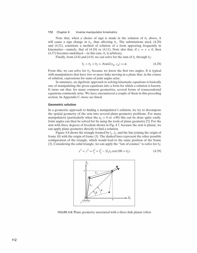
112 Chapter 4 Inverse manipulator kinematics
Note that, when a choice of sign is made in the solution of θ2 above, itwill cause a sign change in k2, thus affecting θ1. The substitutions used, (4.20)and (4.21), constitute a method of solution of a form appearing frequently inkinematics—namely, that of (4.10) or (4.11). Note also that, if x = y = 0, then(4.27) becomes undefined—in this case, θ1 is arbitrary.
Finally, from (4.8) and (4.9), we can solve for the sum of θ1 through θ3:
θ1 + θ2 + θ3 = Atan2(sφ, cφ) = φ. (4.28)
From this, we can solve for θ3, because we know the first two angles. It is typicalwith manipulators that have two or more links moving in a plane that, in the courseof solution, expressions for sums of joint angles arise.
In summary, an algebraic approach to solving kinematic equations is basicallyone of manipulating the given equations into a form for which a solution is known.It turns out that, for many common geometries, several forms of transcendentalequations commonly arise. We have encountered a couple of them in this precedingsection. In Appendix C, more are listed.
Geometric solution
In a geometric approach to finding a manipulator’s solution, we try to decomposethe spatial geometry of the arm into several plane-geometry problems. For manymanipulators (particularly when the αi = 0 or ±90) this can be done quite easily.Joint angles can then be solved for by using the tools of plane geometry [7]. For thearm with three degrees of freedom shown in Fig. 4.7, because the arm is planar, wecan apply plane geometry directly to find a solution.
Figure 4.8 shows the triangle formed by l1, l2, and the line joining the origin offrame {0} with the origin of frame {3}. The dashed lines represent the other possibleconfiguration of the triangle, which would lead to the same position of the frame{3}. Considering the solid triangle, we can apply the ‘‘law of cosines’’ to solve for θ2:
x2 + y2 = l21
+ l22
− 2l1l2 cos(180 + θ2). (4.29)
X0
Y0
L2
L1
x
bc
y
FIGURE 4.8: Plane geometry associated with a three-link planar robot.
112
Section 4.5 Algebraic solution by reduction to polynomial 113
Now; cos(180 + θ2) = − cos(θ2), so we have
c2 =x2 + y2 − l2
1− l2
2
2l1l2. (4.30)
In order for this triangle to exist, the distance to the goal point√
x2 + y2 must beless than or equal to the sum of the link lengths, l1 + l2. This condition would bechecked at this point in a computational algorithm to verify existence of solutions.This condition is not satisfied when the goal point is out of reach of the manipulator.Assuming a solution exists, this equation is solved for that value of θ2 that liesbetween 0 and −180 degrees, because only for these values does the triangle inFig. 4.8 exist. The other possible solution (the one indicated by the dashed-linetriangle) is found by symmetry to be θ ′
2= −θ2.
To solve for θ1, we find expressions for angles ψ and β as indicated in Fig. 4.8.First, β may be in any quadrant, depending on the signs of x and y. So we must usea two-argument arctangent:
β = Atan2(y, x). (4.31)
We again apply the law of cosines to find ψ :
cos ψ =x2 + y2 + l2
1− l2
2
2l1√
x2 + y2. (4.32)
Here, the arccosine must be solved so that 0 ≤ ψ ≤ 180◦, in order that the geometrywhich leads to (4.32) will be preserved. These considerations are typical when usinga geometric approach—we must apply the formulas we derive only over a range ofvariables such that the geometry is preserved. Then we have
θ1 = β ± ψ, (4.33)
where the plus sign is used if θ2 < 0 and the minus sign if θ2 > 0.We know that angles in a plane add, so the sum of the three joint angles must
be the orientation of the last link:
θ1 + θ2 + θ3 = φ. (4.34)
This equation is solved for θ3 to complete our solution.
4.5 ALGEBRAIC SOLUTION BY REDUCTION TO POLYNOMIAL
Transcendental equations are often difficult to solve because, even when there is onlyone variable (say, θ), it generally appears as sin θ and cos θ . Making the followingsubstitutions, however, yields an expression in terms of a single variable, u:
u = tanθ
2,
cos θ = 1 − u2
1 + u2, (4.35)
sin θ = 2u
1 + u2.
113

114 Chapter 4 Inverse manipulator kinematics
This is a very important geometric substitution used often in solving kinematicequations. These substitutions convert transcendental equations into polynomialequations in u. Appendix A lists these and other trigonometric identities.
EXAMPLE 4.3
Convert the transcendental equation
a cos θ + b sin θ = c (4.36)
into a polynomial in the tangent of the half angle, and solve for θ .Substituting from (4.35) and multiplying through by 1 + u2, we have
a(1 − u2) + 2bu = c(1 + u2). (4.37)
Collecting powers of u yields
(a + c)u2 − 2bu + (c − a) = 0, (4.38)
which is solved by the quadratic formula:
u = b ±√
b2 + a2 − c2
a + c. (4.39)
Hence,
θ = 2 tan−1
(
b ±√
b2 + a2 − c2
a + c
)
. (4.40)
Should the solution for u from (4.39) be complex, there is no real solution tothe original transcendental equation. Note that, if a + c = 0, the argument of thearctangent becomes infinity and hence θ = 180◦. In a computer implementation,this potential division by zero should be checked for ahead of time. This situationresults when the quadratic term of (4.38) vanishes, so that the quadratic degeneratesinto a linear equation.
Polynomials up to degree four possess closed-form solutions [8, 9], so manip-ulators sufficiently simple that they can be solved by algebraic equations of thisdegree (or lower) are called closed-form-solvable manipulators.
4.6 PIEPER’S SOLUTION WHEN THREE AXES INTERSECT
As mentioned earlier, although a completely general robot with six degrees offreedom does not have a closed-form solution, certain important special casescan be solved. Pieper [3, 4] studied manipulators with six degrees of freedom inwhich three consecutive axes intersect at a point.2 In this section, we outline themethod he developed for the case of all six joints revolute, with the last three axesintersecting. His method applies to other configurations, which include prismatic
2Included in this family of manipulators are those with three consecutive parallel axes, because theymeet at the point at infinity.
114

Section 4.6 Pieper’s solution when three axes intersect 115
joints, and the interested reader should see [4]. Pieper’s work applies to the majorityof commercially available industrial robots.
When the last three axes intersect, the origins of link frames {4}, {5}, and {6}are all located at this point of intersection. This point is given in base coordinates as
0P4ORG = 01T 1
2T 2
3T 3P4ORG =
x
y
z
1
, (4.41)
or, using the fourth column of (3.6) for i = 4, as
0P4ORG = 01T 1
2T 2
3T
a3−d4sα3d4cα3
1
, (4.42)
or as
0P4ORG = 01T 1
2T
f1(θ3)
f2(θ3)
f3(θ3)
1
, (4.43)
where
f1f2f31
= 23T
a3−d4sα3d4cα3
1
. (4.44)
Using (3.6) for 23T in (4.44) yields the following expressions for f1:
f1 = a3c3 + d4sα3s3 + a2,
f2 = a3cα2s3 − d4sα3cα2c3 − d4sα2cα3 − d3sα2, (4.45)
f3 = a3sα2s3 − d4sα3sα2c3 + d4cα2cα3 + d3cα2.
Using (3.6) for 01T and 1
2T in (4.43), we obtain
0P4ORG =
c1g1 − s1g2s1g1 + c1g2
g31
, (4.46)
where
g1 = c2f1 − s2f2 + a1,
g2 = s2cα1f1 + c2cα1f2 − sα1f3 − d2sα1, (4.47)
g3 = s2sα1f1 + c2sα1f2 + cα1f3 + d2cα1.
We now write an expression for the squared magnitude of 0P4ORG, which we willdenote as r = x2 + y2 + z2, and which is seen from (4.46) to be
r = g21
+ g22
+ g23; (4.48)
115
116 Chapter 4 Inverse manipulator kinematics
so, using (4.47) for the gi , we have
r = f 21
+ f 22
+ f 23
+ a21
+ d22
+ 2d2f3 + 2a1(c2f1 − s2f2). (4.49)
We now write this equation, along with the Z-component equation from (4.46), as asystem of two equations in the form
r = (k1c2 + k2s2)2a1 + k3,
z = (k1s2 − k2c2)sα1 + k4, (4.50)
where
k1 = f1,
k2 = −f2,
k3 = f 21
+ f 22
+ f 23
+ a21
+ d22
+ 2d2f3, (4.51)
k4 = f3cα1 + d2cα1.
Equation (4.50) is useful because dependence on θ1 has been eliminated and becausedependence on θ2 takes a simple form.
Now let us consider the solution of (4.50) for θ3. We distinguish three cases:
1. If a1 = 0, then we have r = k3, where r is known. The right-hand side (k3) is a
function of θ3 only. After the substitution (4.35), a quadratic equation in tanθ32
may be solved for θ3.
2. If sα1 = 0, then we have z = k4, where z is known. Again, after substitutingvia (4.35), a quadratic equation arises that can be solved for θ3.
3. Otherwise, eliminate s2 and c2 from (4.50) to obtain
(r − k3)2
4a21
+ (z − k4)2
s2α1
= k21
+ k22. (4.52)
This equation, after the (4.35) substitution for θ3, results in an equation ofdegree 4, which can be solved for θ3.3
Having solved for θ3, we can solve (4.50) for θ2 and (4.46) for θ1.To complete our solution, we need to solve for θ4, θ5, and θ6. These axes
intersect, so these joint angles affect the orientation of only the last link. We cancompute them from nothing more than the rotation portion of the specified goal,06R. Having obtained θ1, θ2, and θ3, we can compute 0
4R|θ4=0, by which notation we
mean the orientation of link frame {4} relative to the base frame when θ4 = 0. Thedesired orientation of {6} differs from this orientation only by the action of the lastthree joints. Because the problem was specified as given 0
6R, we can compute
46R|θ4=0 = 0
4R−1|θ4=0
06R. (4.53)
3It is helpful to note that f 21
+ f 22
+ f 23
= a23
+ d24
+ d23
+ a22
+ 2d4d3cα3 + 2a2a3c3 + 2a2d4sα3s3.
116
Section 4.7 Examples of inverse manipulator kinematics 117
For many manipulators, these last three angles can be solved for by usingexactly the Z–Y–Z Euler angle solution given in Chapter 2, applied to 4
6R|θ4=0.
For any manipulator (with intersecting axes 4, 5, and 6), the last three joint anglescan be solved for as a set of appropriately defined Euler angles. There are alwaystwo solutions for these last three joints, so the total number of solutions for themanipulator will be twice the number found for the first three joints.
4.7 EXAMPLES OF INVERSE MANIPULATOR KINEMATICS
In this section, we work out the inverse kinematics of two industrial robots. Onemanipulator solution is done purely algebraically; the second solution is partiallyalgebraic and partially geometric. The following solutions do not constitute acookbook method of solving manipulator kinematics, but they do show many ofthe common manipulations likely to appear in most kinematic solutions. Note thatPieper’s method of solution (covered in the preceding section) can be used for thesemanipulators, but here we choose to approach the solution a different way, to giveinsight into various available methods.
The Unimation PUMA 560
As an example of the algebraic solution technique applied to a manipulator with sixdegrees of freedom, we will solve the kinematic equations of the PUMA 560, whichwere developed in Chapter 3. This solution is in the style of [5].
We wish to solve
06T =
r11 r12 r13 px
r21 r22 r23 py
r31 r32 r33 pz
0 0 0 1
= 01T (θ1)
12T (θ2)
23T (θ3)
34T (θ4)
45T (θ5)
56T (θ6) (4.54)
for θi when 06T is given as numeric values.
A restatement of (4.54) that puts the dependence on θ1 on the left-hand sideof the equation is
[01T (θ1)]−1 0
6T = 1
2T (θ2)
23T (θ3)
34T (θ4)
45T (θ5)
56T (θ6). (4.55)
Inverting 01T , we write (4.55) as
c1 s1 0 0−s1 c1 0 0
0 0 1 00 0 0 1
r11 r12 r13 px
r21 r22 r23 py
r31 r32 r33 pz
0 0 0 1
= 16T , (4.56)
where 16T is given by equation (3.13) developed in Chapter 3. This simple technique
of multiplying each side of a transform equation by an inverse is often used toadvantage in separating out variables in the search for a solvable equation.
Equating the (2, 4) elements from both sides of (4.56), we have
−s1px + c1py = d3. (4.57)
117
118 Chapter 4 Inverse manipulator kinematics
To solve an equation of this form, we make the trigonometric substitutions
px = ρ cos φ,
py = ρ sin φ, (4.58)
where
ρ =√
p2x
+ p2y,
φ = Atan2(py, px). (4.59)
Substituting (4.58) into (4.57), we obtain
c1sφ − s1cφ = d3
ρ. (4.60)
From the difference-of-angles formula,
sin(φ − θ1) = d3
ρ. (4.61)
Hence,
cos(φ − θ1) = ±
√
1 −d2
3
ρ2, (4.62)
and so
φ − θ1 = Atan2
d3
ρ,±
√
1 −d2
3
ρ2
. (4.63)
Finally, the solution for θ1 may be written as
θ1 = Atan2(py, px) − Atan2(
d3,±√
p2x
+ p2y
− d23
)
. (4.64)
Note that we have found two possible solutions for θ1, corresponding to the plus-or-minus sign in (4.64). Now that θ1 is known, the left-hand side of (4.56) is known.If we equate both the (1,4) elements and the (3,4) elements from the two sides of(4.56), we obtain
c1px + s1py = a3c23 − d4s23 + a2c2,
−px = a3s23 + d4c23 + a2s2. (4.65)
If we square equations (4.65) and (4.57) and add the resulting equations, we obtain
a3c3 − d4s3 = K, (4.66)
where
K =p2
x+ p2
y+ p2
x− a2
2− a2
3− d2
3− d2
4
2a2
. (4.67)
118

Section 4.7 Examples of inverse manipulator kinematics 119
Note that dependence on θ1 has been removed from (4.66). Equation (4.66) is ofthe same form as (4.57) and so can be solved by the same kind of trigonometricsubstitution to yield a solution for θ3:
θ3 = Atan2(a3, d4) − Atan2(K,±√
a23
+ d24
− K2). (4.68)
The plus-or-minus sign in (4.68) leads to two different solutions for θ3. If we consider(4.54) again, we can now rewrite it so that all the left-hand side is a function of onlyknowns and θ2:
[03T (θ2)]−10
6T = 3
4T (θ4)
45T (θ5)
56T (θ6), (4.69)
or
c1c23 s1c23 −s23 −a2c3−c1s23 −s1s23 −c23 a2s3−s1 c1 0 −d3
0 0 0 1
r11 r12 r13 px
r21 r22 r23 py
r31 r32 r33 pz
0 0 0 1
= 36T , (4.70)
where 36T is given by equation (3.11) developed in Chapter 3. Equating both
the (1,4) elements and the (2,4) elements from the two sides of (4.70), we get
c1c23px + s1c23py − s23pz − a2c3 = a3,
−c1s23px − s1s23py − c23pz + a2s3 = d4. (4.71)
These equations can be solved simultaneously for s23 and c23, resulting in
s23 =(−a3 − a2c3)pz + (c1px + s1py)(a2s3 − d4)
p2z
+ (c1px + s1py)2
,
c23 =(a2s3 − d4)pz − (a3 + a2c3)(c1px + s1py)
p2z
+ (c1px + s1py)2
. (4.72)
The denominators are equal and positive, so we solve for the sum of θ2 and θ3 as
θ23 = Atan2[(−a3 − a2c3)pz − (c1px + s1py)(d4 − a2s3),
(a2s3 − d4)pz − (a3 + a2c3)(c1px + s1py)]. (4.73)
Equation (4.73) computes four values of θ23, according to the four possible combina-tions of solutions for θ1 and θ3; then, four possible solutions for θ2 are computed as
θ2 = θ23 − θ3, (4.74)
where the appropriate solution for θ3 is used when forming the difference.Now the entire left side of (4.70) is known. Equating both the (1,3) elements
and the (3,3) elements from the two sides of (4.70), we get
r13c1c23 + r23s1c23 − r33s23 = −c4s5,
−r13s1 + r23c1 = s4s5. (4.75)
As long as s5 �= 0, we can solve for θ4 as
θ4 = Atan2(−r13s1 + r23c1,−r13c1c23 − r23s1c23 + r33s23). (4.76)
119

120 Chapter 4 Inverse manipulator kinematics
When θ5 = 0, the manipulator is in a singular configuration in which joint axes 4 and6 line up and cause the same motion of the last link of the robot. In this case, all thatmatters (and all that can be solved for) is the sum or difference of θ4 and θ6. Thissituation is detected by checking whether both arguments of the Atan2 in (4.76) arenear zero. If so, θ4 is chosen arbitrarily,4 and when θ6 is computed later, it will becomputed accordingly.
If we consider (4.54) again, we can now rewrite it so that all the left-hand sideis a function of only knowns and θ4, by rewriting it as
[04T (θ4)]
−1 06T = 4
5T (θ5)
56T (θ6), (4.77)
where [04T (θ4)]−1 is given by
c1c23c4 + s1s4 s1c23c4 − c1s4 −s23c4 −a2c3c4 + d3s4 − a3c4−c1c23s4 + s1c4 −s1c23s4 − c1c4 s23s4 a2c3s4 + d3c4 + a3s4
−c1s23 −s1s23 −c23 a2s3 − d40 0 0 1
, (4.78)
and 46T is given by equation (3.10) developed in Chapter 3. Equating both the (1,3)
elements and the (3,3) elements from the two sides of (4.77), we get
r13(c1c23c4 + s1s4) + r23(s1c23c4 − c1s4) − r33(s23c4) = −s5,
r13(−c1s23) + r23(−s1s23) + r33(−c23) = c5. (4.79)
Hence, we can solve for θ5 as
θ5 = Atan2(s5, c5), (4.80)
where s5 and c5 are given by (4.79).Applying the same method one more time, we compute (0
5T )−1 and write
(4.54) in the form
(05T )−1 0
6T = 5
6T (θ6). (4.81)
Equating both the (3,1) elements and the (1,1) elements from the two sides of (4.77)as we have done before, we get
θ6 = Atan2(s6, c6), (4.82)
where
s6 = −r11(c1c23s4 − s1c4) − r21(s1c23s4 + c1c4) + r31(s23s4),
c6 = r11[(c1c23c4 + s1s4)c5 − c1s23s5] + r21[(s1c23c4 − c1s4)c5 − s1s23s5]−r31(s23c4c5 + c23s5).
Because of the plus-or-minus signs appearing in (4.64) and (4.68), these equationscompute four solutions. Additionally, there are four more solutions obtained by
4It is usually chosen to be equal to the present value of joint 4.
120
Section 4.7 Examples of inverse manipulator kinematics 121
‘‘flipping’’ the wrist of the manipulator. For each of the four solutions computedabove, we obtain the flipped solution by
θ ′4
= θ4 + 180◦,
θ ′5
= −θ5, (4.83)
θ ′6
= θ6 + 180◦.
After all eight solutions have been computed, some (or even all) of them might haveto be discarded because of joint-limit violations. Of any remaining valid solutions,usually the one closest to the present manipulator configuration is chosen.
The Yasukawa Motoman L-3
As the second example, we will solve the kinematic equations of the YasukawaMotoman L-3, which were developed in Chapter 3. This solution will be partiallyalgebraic and partially geometric. The Motoman L-3 has three features that makethe inverse kinematic problem quite different from that of the PUMA. First, themanipulator has only five joints, so it is not able to position and orient its end-effector in order to attain general goal frames. Second, the four-bar type of linkagesand chain-drive scheme cause one actuator to move two or more joints. Third, theactuator position limits are not constants, but depend on the positions of the otheractuators, so finding out whether a computed set of actuator values is in range is nottrivial.
If we consider the nature of the subspace of the Motoman manipulator (andthe same applies to many manipulators with five degrees of freedom), we quicklyrealize that this subspace can be described by giving one constraint on the attainableorientation: The pointing direction of the tool, that is, the ZT axis, must lie in the‘‘plane of the arm.’’ This plane is the vertical plane that contains the axis of joint1 and the point where axes 4 and 5 intersect. The orientation nearest to a generalorientation is the one obtained by rotating the tool’s pointing direction so that it liesin the plane, using a minimum amount of rotation. Without developing an explicitexpression for this subspace, we will construct a method for projecting a generalgoal frame into it. Note that this entire discussion is for the case that the wrist frameand tool frame differ only by a translation along Zw.
In Fig. 4.9, we indicate the plane of the arm by its normal, M , and the desiredpointing direction of the tool by ZT . This pointing direction must be rotated by
angle θ about some vector K in order to cause the new pointing direction, Z′T
, to lie
in the plane. It is clear that the K that minimizes θ lies in the plane and is orthogonalto both ZT and Z′
T.
For any given goal frame, M is defined as
M = 1√
p2x
+ p2y
−py
px
0
, (4.84)
where px and py are the X and Y coordinates of the desired tool position. Then K
is given byK = M × ZT . (4.85)
121
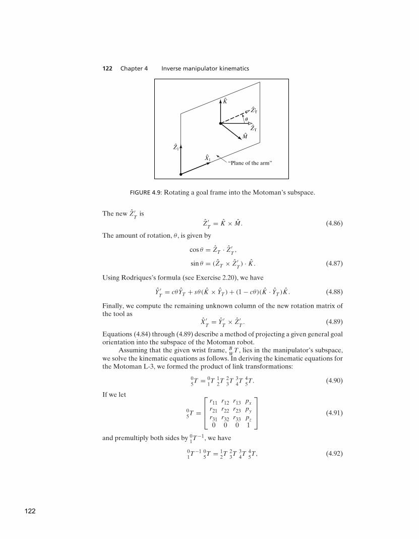
122 Chapter 4 Inverse manipulator kinematics
“Plane of the arm”X1
u
K
M
Z1
Z�T
ZT
FIGURE 4.9: Rotating a goal frame into the Motoman’s subspace.
The new Z′T
is
Z′T
= K × M. (4.86)
The amount of rotation, θ , is given by
cos θ = ZT · Z′T,
sin θ = (ZT × Z′T) · K. (4.87)
Using Rodriques’s formula (see Exercise 2.20), we have
Y ′T
= cθYT + sθ(K × YT ) + (1 − cθ)(K · YT )K. (4.88)
Finally, we compute the remaining unknown column of the new rotation matrix ofthe tool as
X′T
= Y ′T
× Z′T. (4.89)
Equations (4.84) through (4.89) describe a method of projecting a given general goalorientation into the subspace of the Motoman robot.
Assuming that the given wrist frame, BW
T , lies in the manipulator’s subspace,we solve the kinematic equations as follows. In deriving the kinematic equations forthe Motoman L-3, we formed the product of link transformations:
05T = 0
1T 1
2T 2
3T 3
4T 4
5T . (4.90)
If we let
05T =
r11 r12 r13 px
r21 r22 r23 py
r31 r32 r33 pz
0 0 0 1
(4.91)
and premultiply both sides by 01T −1, we have
01T −1 0
5T = 1
2T 2
3T 3
4T 4
5T , (4.92)
122
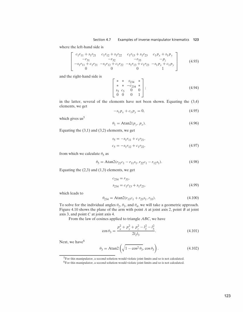
Section 4.7 Examples of inverse manipulator kinematics 123
where the left-hand side is
c1r11 + s1r21 c1r12 + s1r22 c1r13 + s1r23 c1px + s1py
−r31 −r32 −r33 −pz
−s1r11 + c1r21 −s1r12 + c1r22 −s1r13 + c1r23 −s1px + c1py
0 0 0 1
(4.93)
and the right-hand side is
∗ ∗ s234 ∗∗ ∗ −c234 ∗s5 c5 0 00 0 0 1
; (4.94)
in the latter, several of the elements have not been shown. Equating the (3,4)elements, we get
−s1px + c1py = 0, (4.95)
which gives us5
θ1 = Atan2(py, px). (4.96)
Equating the (3,1) and (3,2) elements, we get
s5 = −s1r11 + c1r21,
c5 = −s1r12 + c1r22, (4.97)
from which we calculate θ5 as
θ5 = Atan2(r21c1 − r11s1, r22c1 − r12s1). (4.98)
Equating the (2,3) and (1,3) elements, we get
c234 = r33,
s234 = c1r13 + s1r23, (4.99)
which leads toθ234 = Atan2(r13c1 + r23s1, r33). (4.100)
To solve for the individual angles θ2, θ3, and θ4, we will take a geometric approach.Figure 4.10 shows the plane of the arm with point A at joint axis 2, point B at jointaxis 3, and point C at joint axis 4.
From the law of cosines applied to triangle ABC, we have
cos θ3 =p2
x+ p2
y+ p2
z− l2
2− l2
3
2l2l3. (4.101)
Next, we have6
θ3 = Atan2
(
√
1 − cos2 θ3, cos θ3
)
. (4.102)
5For this manipulator, a second solution would violate joint limits and so is not calculated.6For this manipulator, a second solution would violate joint limits and so is not calculated.
123
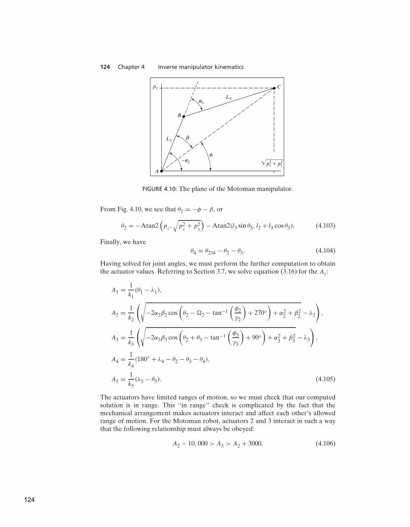
124 Chapter 4 Inverse manipulator kinematics
B
A
pz
b
f
u3
L2
L3
C
�u2 �p2x � p2
y
FIGURE 4.10: The plane of the Motoman manipulator.
From Fig. 4.10, we see that θ2 = −φ − β, or
θ2 = −Atan2(
pz,√
p2x
+ p2y
)
− Atan2(l3 sin θ3, l2 + l3 cos θ3). (4.103)
Finally, we have
θ4 = θ234 − θ2 − θ3. (4.104)
Having solved for joint angles, we must perform the further computation to obtainthe actuator values. Referring to Section 3.7, we solve equation (3.16) for the Ai :
A1 = 1
k1
(θ1 − λ1),
A2 = 1
k2
(√
−2α2β2 cos
(
θ2 − 12 − tan−1
(
φ2
γ2
)
+ 270◦)
+ α22
+ β22
− λ2
)
,
A3 = 1
k3
(√
−2α3β3 cos
(
θ2 + θ3 − tan−1
(
φ3
γ3
)
+ 90◦)
+ α23
+ β23
− λ3
)
,
A4 = 1
k4
(180◦ + λ4 − θ2 − θ3 − θ4),
A5 = 1
k5
(λ5 − θ5). (4.105)
The actuators have limited ranges of motion, so we must check that our computedsolution is in range. This ‘‘in range’’ check is complicated by the fact that themechanical arrangement makes actuators interact and affect each other’s allowedrange of motion. For the Motoman robot, actuators 2 and 3 interact in such a waythat the following relationship must always be obeyed:
A2 − 10, 000 > A3 > A2 + 3000. (4.106)
124

Section 4.8 The standard frames 125
That is, the limits of actuator 3 are a function of the position of actuator 2. Similarly,
32,000 − A4 < A5 < 55,000. (4.107)
Now, one revolution of joint 5 corresponds to 25,600 actuator counts, so, whenA4 > 2600, there are two possible solutions for A5. This is the only situation in whichthe Yasukawa Motoman L-3 has more than one solution.
4.8 THE STANDARD FRAMES
The ability to solve for joint angles is really the central element in many robotcontrol systems. Again, consider the paradigm indicated in Fig. 4.11, which showsthe standard frames.
The way these frames are used in a general robot system is as follows:
1. The user specifies to the system where the station frame is to be located. Thismight be at the corner of a work surface, as in Fig. 4.12, or even affixed to amoving conveyor belt. The station frame, {S}, is defined relative to the baseframe, {B}.
2. The user specifies the description of the tool being used by the robot by givingthe {T }-frame specification. Each tool the robot picks up could have a different{T } frame associated with it. Note that the same tool grasped in different waysrequires different {T }-frame definitions. {T } is specified relative to {W }—thatis, W
TT .
3. The user specifies the goal point for a robot motion by giving the descriptionof the goal frame, {G}, relative to the station frame. Often, the definitions of{T } and {S} remain fixed for several motions of the robot. In this case, oncethey are defined, the user simply gives a series of {G} specifications.
�B ��W �
�S � �G �
�T �
FIGURE 4.11: Location of the ‘‘standard’’ frames.
125

126 Chapter 4 Inverse manipulator kinematics
Goalframe
Stationframe
Base frame
Wrist frame
Tool frame
Pin
Camera
FIGURE 4.12: Example workstation.
In many systems, the tool frame definition (WT
T ) is constant (for example, it isdefined with its origin at the center of the fingertips). Also, the station framemight be fixed or might easily be taught by the user with the robot itself. Insuch systems, the user need not be aware of the five standard frames—he orshe simply thinks in terms of moving the tool to locations (goals) with respectto the work area specified by station frame.
4. The robot system calculates a series of joint angles to move the joints throughin order that the tool frame will move from its initial location in a smoothmanner until {T } = {G} at the end of motion.
4.9 SOLVE-ING A MANIPULATOR
The SOLVE function implements Cartesian transformations and calls the inversekinematics function. Thus, the inverse kinematics are generalized so that arbi-trary tool-frame and station-frame definitions may be used with our basic inversekinematics, which solves for the wrist frame relative to the base frame.
Given the goal-frame specification, STT , SOLVE uses the tool and station
definitions to calculate the location of {W } relative to {B}, BW
T :
B
WT = B
ST S
TT W
TT −1. (4.108)
Then, the inverse kinematics take BW
T as an input and calculate θ1 through θn.
126
Section 4.11 Computational considerations 127
4.10 REPEATABILITY AND ACCURACY
Many industrial robots today move to goal points that have been taught. A taught
point is one that the manipulator is moved to physically, and then the joint positionsensors are read and the joint angles stored. When the robot is commanded toreturn to that point in space, each joint is moved to the stored value. In simple‘‘teach and playback’’ manipulators such as these, the inverse kinematic problemnever arises, because goal points are never specified in Cartesian coordinates. Whena manufacturer specifies how precisely a manipulator can return to a taught point,he is specifying the repeatability of the manipulator.
Any time a goal position and orientation are specified in Cartesian terms,the inverse kinematics of the device must be computed in order to solve for therequired joint angles. Systems that allow goals to be described in Cartesian termsare capable of moving the manipulator to points that were never taught—points inits workspace to which it has perhaps never gone before. We will call such pointscomputed points. Such a capability is necessary for many manipulation tasks. Forexample, if a computer vision system is used to locate a part that the robot mustgrasp, the robot must be able to move to the Cartesian coordinates supplied by thevision sensor. The precision with which a computed point can be attained is calledthe accuracy of the manipulator.
The accuracy of a manipulator is bounded by the repeatability. Clearly,accuracy is affected by the precision of parameters appearing in the kinematicequations of the robot. Errors in knowledge of the Denavit–Hartenberg parameterswill cause the inverse kinematic equations to calculate joint angle values that arein error. Hence, although the repeatability of most industrial manipulators is quitegood, the accuracy is usually much worse and varies quite a bit from manipulatorto manipulator. Calibration techniques can be devised that allow the accuracy ofa manipulator to be improved through estimation of that particular manipulator’skinematic parameters [10].
4.11 COMPUTATIONAL CONSIDERATIONS
In many path-control schemes, which we will consider in Chapter 7, it is necessaryto calculate the inverse kinematics of a manipulator at fairly high rates, for exam-ple, 30 Hz or faster. Therefore, computational efficiency is an issue. These speedrequirements rule out the use of numerical-solution techniques that are iterative innature; for this reason, we have not considered them.
Most of the general comments of Section 3.10, made for forward kinematics,also hold for the problem of inverse kinematics. For the inverse-kinematic case, atable-lookup Atan2 routine is often used to attain higher speeds.
Structure of the computation of multiple solutions is also important. It isgenerally fairly efficient to generate all of them in parallel, rather than pursuing oneafter another serially. Of course, in some applications, when all solutions are notrequired, substantial time is saved by computing only one.
When a geometric approach is used to develop an inverse-kinematic solution,it is sometimes possible to calculate multiple solutions by simple operations on thevarious angles solved for in obtaining the first solution. That is, the first solution
127

128 Chapter 4 Inverse manipulator kinematics
is moderately expensive computationally, but the other solutions are found veryquickly by summing and differencing angles, subtracting π , and so on.
BIBLIOGRAPHY
[1] B. Roth, J. Rastegar, and V. Scheinman, ‘‘On the Design of Computer ControlledManipulators,’’ On the Theory and Practice of Robots and Manipulators, Vol. 1, FirstCISM-IFToMM Symposium, September 1973, pp. 93–113.
[2] B. Roth, ‘‘Performance Evaluation of Manipulators from a Kinematic Viewpoint,’’ Per-
formance Evaluation of Manipulators, National Bureau of Standards, special publication,1975.
[3] D. Pieper and B. Roth, ‘‘The Kinematics of Manipulators Under Computer Control,’’Proceedings of the Second International Congress on Theory of Machines and Mechanisms,Vol. 2, Zakopane, Poland, 1969, pp. 159–169.
[4] D. Pieper, ‘‘The Kinematics of Manipulators Under Computer Control,’’ UnpublishedPh.D. Thesis, Stanford University, 1968.
[5] R.P. Paul, B. Shimano, and G. Mayer, ‘‘Kinematic Control Equations for Simple Manip-ulators,’’ IEEE Transactions on Systems, Man, and Cybernetics, Vol. SMC-11, No. 6,1981.
[6] L. Tsai and A. Morgan, ‘‘Solving the Kinematics of the Most General Six- and Five-degree-of-freedom Manipulators by Continuation Methods,’’ Paper 84-DET-20, ASMEMechanisms Conference, Boston, October 7–10, 1984.
[7] C.S.G. Lee and M. Ziegler, ‘‘Geometric Approach in Solving Inverse Kinematics ofPUMA Robots,’’ IEEE Transactions on Aerospace and Electronic Systems, Vol. AES-20,No. 6, November 1984.
[8] W. Beyer, CRC Standard Mathematical Tables, 25th edition, CRC Press, Inc., BocaRaton, FL, 1980.
[9] R. Burington, Handbook of Mathematical Tables and Formulas, 5th edition, McGraw-Hill, New York, 1973.
[10] J. Hollerbach, ‘‘A Survey of Kinematic Calibration,’’ in The Robotics Review, O. Khatib,J. Craig, and T. Lozano-Perez, Editors, MIT Press, Cambridge, MA, 1989.
[11] Y. Nakamura and H. Hanafusa, ‘‘Inverse Kinematic Solutions with Singularity Robust-ness for Robot Manipulator Control,’’ ASME Journal of Dynamic Systems, Measurement,
and Control, Vol. 108, 1986.
[12] D. Baker and C. Wampler, ‘‘On the Inverse Kinematics of Redundant Manipulators,’’International Journal of Robotics Research, Vol. 7, No. 2, 1988.
[13] L.W. Tsai, Robot Analysis: The Mechanics of Serial and Parallel Manipulators, Wiley,New York, 1999.
EXERCISES
4.1 [15] Sketch the fingertip workspace of the three-link manipulator of Chapter 3,Exercise 3.3 for the case l1 = 15.0, l2 = 10.0, and l3 = 3.0.
4.2 [26] Derive the inverse kinematics of the three-link manipulator of Chapter 3,Exercise 3.3.
4.3 [12] Sketch the fingertip workspace of the 3-DOF manipulator of Chapter 3,Example 3.4.
128
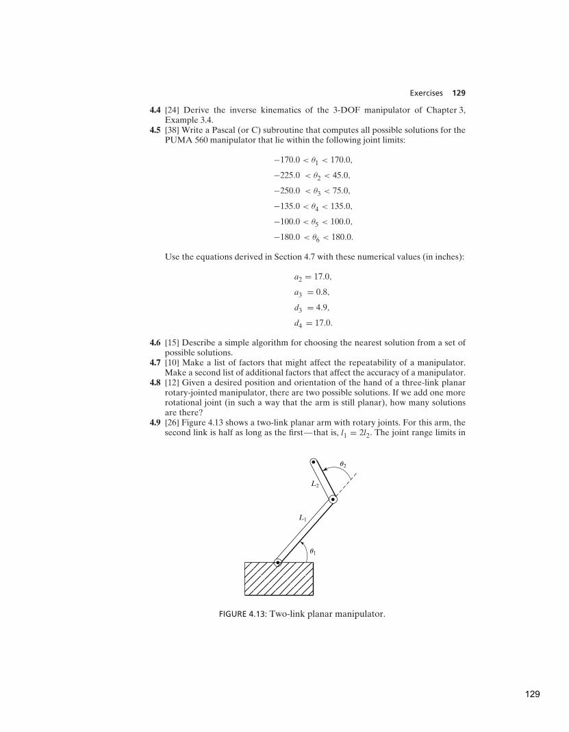
Exercises 129
4.4 [24] Derive the inverse kinematics of the 3-DOF manipulator of Chapter 3,Example 3.4.
4.5 [38] Write a Pascal (or C) subroutine that computes all possible solutions for thePUMA 560 manipulator that lie within the following joint limits:
−170.0 < θ1 < 170.0,
−225.0 < θ2 < 45.0,
−250.0 < θ3 < 75.0,
−135.0 < θ4 < 135.0,
−100.0 < θ5 < 100.0,
−180.0 < θ6 < 180.0.
Use the equations derived in Section 4.7 with these numerical values (in inches):
a2 = 17.0,
a3 = 0.8,
d3 = 4.9,
d4 = 17.0.
4.6 [15] Describe a simple algorithm for choosing the nearest solution from a set ofpossible solutions.
4.7 [10] Make a list of factors that might affect the repeatability of a manipulator.Make a second list of additional factors that affect the accuracy of a manipulator.
4.8 [12] Given a desired position and orientation of the hand of a three-link planarrotary-jointed manipulator, there are two possible solutions. If we add one morerotational joint (in such a way that the arm is still planar), how many solutionsare there?
4.9 [26] Figure 4.13 shows a two-link planar arm with rotary joints. For this arm, thesecond link is half as long as the first—that is, l1 = 2l2. The joint range limits in
u1
u2
L1
L2
FIGURE 4.13: Two-link planar manipulator.
129

130 Chapter 4 Inverse manipulator kinematics
degrees are
0 < θ1 < 180,
−90 < θ2 < 180.
Sketch the approximate reachable workspace (an area) of the tip of link 2.4.10 [23] Give an expression for the subspace of the manipulator of Chapter 3,
Example 3.4.4.11 [24] A 2-DOF positioning table is used to orient parts for arc-welding. The
forward kinematics that locate the bed of the table (link 2) with respect to thebase (link 0) are
02T =
c1c2 −c1s2 s1 l2s1 + l1s2 c2 0 0
−s1c2 s1s2 c1 l2c1 + h10 0 0 1
.
Given any unit direction fixed in the frame of the bed (link 2), 2V , give theinverse-kinematic solution for θ1, θ2 such that this vector is aligned with 0Z (i.e.,upward). Are there multiple solutions? Is there a singular condition for which aunique solution cannot be obtained?
4.12 [22] In Fig. 4.14, two 3R mechanisms are pictured. In both cases, the three axesintersect at a point (and, over all configurations, this point remains fixed in space).The mechanism in Fig. 4.14(a) has link twists (αi) of magnitude 90 degrees. Themechanism in Fig. 4.14(b) has one twist of φ in magnitude and the other of 180−φ
in magnitude.The mechanism in Fig. 4.14(a) can be seen to be in correspondence with Z–Y–ZEuler angles, and therefore we know that it suffices to orient link 3 (with arrowin figure) arbitrarily with respect to the fixed link 0. Because φ is not equal to 90degrees, it turns out that the other mechanism cannot orient link 3 arbitrarily.
u3
u1
u2
(a) (b)
u3
u2
u2
f
FIGURE 4.14: Two 3R mechanisms (Exercise 4.12).
130
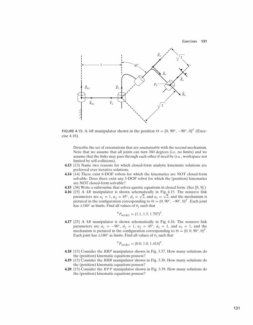
Exercises 131
1
Z0,1
X0,1 Y2
X3
X4^
Z3
Z4
Z2
P4
2
2
45
FIGURE 4.15: A 4R manipulator shown in the position 5 = [0, 90◦,−90◦, 0]T (Exer-cise 4.16).
Describe the set of orientations that are unattainable with the second mechanism.Note that we assume that all joints can turn 360 degrees (i.e. no limits) and weassume that the links may pass through each other if need be (i.e., workspace notlimited by self-collisions).
4.13 [13] Name two reasons for which closed-form analytic kinematic solutions arepreferred over iterative solutions.
4.14 [14] There exist 6-DOF robots for which the kinematics are NOT closed-formsolvable. Does there exist any 3-DOF robot for which the (position) kinematicsare NOT closed-form solvable?
4.15 [38] Write a subroutine that solves quartic equations in closed form. (See [8, 9].)4.16 [25] A 4R manipulator is shown schematically in Fig. 4.15. The nonzero link
parameters are a1 = 1, α2 = 45◦, d3 =√
2, and a3 =√
2, and the mechanism ispictured in the configuration corresponding to 5 = [0, 90◦,−90◦, 0]T . Each jointhas ±180◦ as limits. Find all values of θ3 such that
0P4ORG = [1.1, 1.5, 1.707]T .
4.17 [25] A 4R manipulator is shown schematically in Fig. 4.16. The nonzero linkparameters are α1 = −90◦, d2 = 1, α2 = 45◦, d3 = 1, and a3 = 1, and themechanism is pictured in the configuration corresponding to 5 = [0, 0, 90◦, 0]T .Each joint has ±180◦ as limits. Find all values of θ3 such that
0P4ORG = [0.0, 1.0, 1.414]T .
4.18 [15] Consider the RRP manipulator shown in Fig. 3.37. How many solutions dothe (position) kinematic equations possess?
4.19 [15] Consider the RRR manipulator shown in Fig. 3.38. How many solutions dothe (position) kinematic equations possess?
4.20 [15] Consider the RPP manipulator shown in Fig. 3.39. How many solutions dothe (position) kinematic equations possess?
131

132 Chapter 4 Inverse manipulator kinematics
Z0,1
Y0,1
Y2
Z2
Z3
Z4
X4
X3
FIGURE 4.16: A 4R manipulator shown in the position 5 = [0, 0, 90◦, 0]T (Exer-cise 4.17).
4.21 [15] Consider the PRR manipulator shown in Fig. 3.40. How many solutions dothe (position) kinematic equations possess?
4.22 [15] Consider the PPP manipulator shown in Fig. 3.41. How many solutions dothe (position) kinematic equations possess?
4.23 [38] The following kinematic equations arise in a certain problem:
sin ξ = a sin θ + b,
sin φ = c cos θ + d,
ψ = ξ + φ.
Given a, b, c, d , and ψ , show that, in the general case, there are four solutions forθ . Give a special condition under which there are just two solutions for θ .
4.24 [20] Given the description of link frame {i} in terms of link frame {i − 1}, find thefour Denavit–Hartenberg parameters as functions of the elements of i−1
iT .
PROGRAMMING EXERCISE (PART 4)
1. Write a subroutine to calculate the inverse kinematics for the three-link manipu-lator of Section 4.4. The routine should pass arguments in the form
Procedure INVKIN(VAR wrelb: frame; VAR current, near, far: vec3;
VAR sol: boolean);
where ‘‘wrelb,’’ an input, is the wrist frame specified relative to the base frame;‘‘current,’’ an input, is the current position of the robot (given as a vector of jointangles); ‘‘near’’ is the nearest solution; ‘‘far’’ is the second solution; and ‘‘sol’’ isa flag that indicates whether solutions were found. (sol = FALSE if no solutionswere found). The link lengths (meters) are
l1 = l2 = 0.5.
132
MATLAB Exercise 4 133
The joint ranges of motion are
−170◦ ≤ θi ≤ 170◦.
Test your routine by calling it back-to-back with KIN to demonstrate that they areindeed inverses of one another.
2. A tool is attached to link 3 of the manipulator. This tool is described by WT
T , thetool frame relative to the wrist frame. Also, a user has described his work area, thestation frame relative to the base of the robot, as B
ST . Write the subroutine
Procedure SOLVE(VAR trels: frame; VAR current, near, far: vec3;
VAR sol: boolean);
where ‘‘trels’’ is the {T } frame specified relative to the {S} frame. Other parametersare exactly as in the INVKIN subroutine. The definitions of {T } and {S} should beglobally defined variables or constants. SOLVE should use calls to TMULT, TINVERT,and INVKIN.
3. Write a main program that accepts a goal frame specified in terms of x, y, and φ.This goal specification is {T } relative to {S}, which is the way the user wants tospecify goals.
The robot is using the same tool in the same working area as in ProgrammingExercise (Part 2), so {T } and {S} are defined as
W
TT = [x y θ] = [0.1 0.2 30.0],
B
ST = [x y θ] = [−0.1 0.3 0.0].
Calculate the joint angles for each of the following three goal frames:
[x1 y1 φ1] = [0.0 0.0 − 90.0],[x2 y2 φ2] = [0.6 − 0.3 45.0],[x3 y3 φ3] = [−0.4 0.3 120.0],[x4 y4 φ4] = [0.8 1.4 30.0].
Assume that the robot will start with all angles equal to 0.0 and move to thesethree goals in sequence. The program should find the nearest solution with respectto the previous goal point. You should call SOLVE and WHERE back-to-back to makesure they are truly inverse functions.
MATLAB EXERCISE 4
This exercise focuses on the inverse-pose kinematics solution for the planar 3-DOF,3R robot. (See Figures 3.6 and 3.7; the DH parameters are given in Figure 3.8.) Thefollowing fixed-length parameters are given: L1 = 4, L2 = 3, and L3 = 2(m).
a) Analytically derive, by hand, the inverse-pose solution for this robot: Given0HT , calculate all possible multiple solutions for {θ1 θ2 θ3}. (Three methods are
presented in the text—choose one of these.) Hint: To simplify the equations, firstcalculate 0
3T from 0
HT and L3.
b) Develop a MATLAB program to solve this planar 3R robot inverse-pose kine-matics problem completely (i.e., to give all multiple solutions). Test your program,using the following input cases:
133

134 Chapter 4 Inverse manipulator kinematics
i) 0HT =
1 0 0 90 1 0 00 0 1 00 0 0 1
.
ii) 0HT =
0.5 −0.866 0 7.53730.866 0.6 0 3.9266
0 0 1 00 0 0 1
.
iii) 0HT =
0 1 0 −3−1 0 0 2
0 0 1 00 0 0 1
.
iv) 0HT =
0.866 0.5 0 −3.1245−0.5 0.866 0 9.1674
0 0 1 00 0 0 1
.
For all cases, employ a circular check to validate your results: Plug each resultingset of joint angles (for each of the multiple solutions) back into the forward-pose kinematics MATLAB program to demonstrate that you get the originallycommanded 0
HT .
c) Check all results by means of the Corke MATLAB Robotics Toolbox. Try functionikine().
134

C H A P T E R 5
Jacobians: velocitiesand static forces
5.1 INTRODUCTION
5.2 NOTATION FOR TIME-VARYING POSITION AND ORIENTATION
5.3 LINEAR AND ROTATIONAL VELOCITY OF RIGID BODIES
5.4 MORE ON ANGULAR VELOCITY
5.5 MOTION OF THE LINKS OF A ROBOT
5.6 VELOCITY ‘‘PROPAGATION’’ FROM LINK TO LINK
5.7 JACOBIANS
5.8 SINGULARITIES
5.9 STATIC FORCES IN MANIPULATORS
5.10 JACOBIANS IN THE FORCE DOMAIN
5.11 CARTESIAN TRANSFORMATION OF VELOCITIES AND STATIC FORCES
5.1 INTRODUCTION
In this chapter, we expand our consideration of robot manipulators beyond static-positioning problems. We examine the notions of linear and angular velocity of arigid body and use these concepts to analyze the motion of a manipulator. We alsowill consider forces acting on a rigid body, and then use these ideas to study theapplication of static forces with manipulators.
It turns out that the study of both velocities and static forces leads to a matrixentity called the Jacobian1 of the manipulator, which will be introduced in thischapter.
The field of kinematics of mechanisms is not treated in great depth here.For the most part, the presentation is restricted to only those ideas which arefundamental to the particular problem of robotics. The interested reader is urged tostudy further from any of several texts on mechanics [1–3].
5.2 NOTATION FOR TIME-VARYING POSITION AND ORIENTATION
Before investigating the description of the motion of a rigid body, we briefly discusssome basics: the differentiation of vectors, the representation of angular velocity,and notation.
1Mathematicians call it the ‘‘Jacobian matrix,’’ but roboticists usually shorten it to simply ‘‘Jacobian.’’
From Chapter 5 of Introduction to Robotics: Mechanics and Control, Third Edition. John J. Craig.
Copyright © 2005 by Pearson Education, Inc. All rights reserved.
135

136 Chapter 5 Jacobians: velocities and static forces
Differentiation of position vectors
As a basis for our consideration of velocities (and, in Chapter 6, accelerations), weneed the following notation for the derivative of a vector:
BVQ =d
dt
BQ = lim�t→0
BQ(t + �t) − BQ(t)
�t. (5.1)
The velocity of a position vector can be thought of as the linear velocity of thepoint in space represented by the position vector. From (5.1), we see that we arecalculating the derivative of Q relative to frame {B}. For example, if Q is notchanging in time relative to {B}, then the velocity calculated is zero—even if thereis some other frame in which Q is varying. Thus, it is important to indicate the framein which the vector is differentiated.
As with any vector, a velocity vector can be described in terms of any frame,and this frame of reference is noted with a leading superscript. Hence, the velocityvector calculated by (5.1), when expressed in terms of frame {A}, would be written
A(BVQ) =Ad
dt
BQ. (5.2)
So we see that, in the general case, a velocity vector is associated with a point inspace, but the numerical values describing the velocity of that point depend on twoframes: one with respect to which the differentiation was done, and one in which theresulting velocity vector is expressed.
In (5.1), the calculated velocity is written in terms of the frame of differentia-tion, so the result could be indicated with a leading B superscript, but, for simplicity,when both superscripts are the same, we needn’t indicate the outer one; that is, wewrite
B(BVQ) = BVQ. (5.3)
Finally, we can always remove the outer, leading superscript by explicitly includ-ing the rotation matrix that accomplishes the change in reference frame (seeSection 2.10); that is, we write
A(BVQ) = A
BR BVQ. (5.4)
We will usually write expressions in the form of the right-hand side of (5.4) so thatthe symbols representing velocities will always mean the velocity in the frame ofdifferentiation and will not have outer, leading superscripts.
Rather than considering a general point’s velocity relative to an arbitraryframe, we will very often consider the velocity of the origin of a frame relativeto some understood universe reference frame. For this special case, we define ashorthand notation,
υC = UVCORG, (5.5)
where the point in question is the origin of frame {C} and the reference frame is{U}. For example, we can use the notation υC to refer to the velocity of the originof frame {C}; then AυC is the velocity of the origin of frame {C} expressed in termsof frame {A} (though differentiation was done relative to {U}).
136

Section 5.2 Notation for time-varying position and orientation 137
{U }
{C }
{T }
ZU
XU
YU
ˆ
ˆ
ˆ
FIGURE 5.1: Example of some frames in linear motion.
EXAMPLE 5.1
Figure 5.1 shows a fixed universe frame, {U}, a frame attached to a train traveling at100 mph, {T }, and a frame attached to a car traveling at 30 mph, {C}. Both vehiclesare heading in the X direction of {U}. The rotation matrices, U
TR and U
CR, are known
and constant.
What isUd
dtUPCORG?
Ud
dt
UPCORG = UVCORG = υC = 30X.
What is C(UVTORG)?
C(UVTORG) = CυT = C
URυT =C
UR(100X) = U
CR−1 100X.
What is C(T VCORG)?
C(T VCORG) = C
TR T VCORG = −U
CR−1 U
TR 70X.
The angular velocity vector
We now introduce an angular velocity vector, using the symbol �. Whereas linearvelocity describes an attribute of a point, angular velocity describes an attribute ofa body. We always attach a frame to the bodies we consider, so we can also think ofangular velocity as describing rotational motion of a frame.
In Fig. 5.2, A�B describes the rotation of frame {B} relative to {A}. Physically,at any instant, the direction of A�B indicates the instantaneous axis of rotation of{B} relative to {A}, and the magnitude of A�B indicates the speed of rotation. Again,like any vector, an angular velocity vector may be expressed in any coordinatesystem, and so another leading superscript may be added; for example, C(A�B) isthe angular velocity of frame {B} relative to {A} expressed in terms of frame {C}.
137

138 Chapter 5 Jacobians: velocities and static forces
{A}{B}
A�B
FIGURE 5.2: Frame {B} is rotating with angular velocity A�B relative to frame {A}.
Again, we introduce a simplified notation for an important special case. Thisis simply the case in which there is an understood reference frame, so that it neednot be mentioned in the notation:
ωC = U�C . (5.6)
Here, ωC is the angular velocity of frame {C} relative to some understood referenceframe, {U}. For example, AωC is the angular velocity of frame {C} expressed in termsof {A} (though the angular velocity is with respect to {U}).
5.3 LINEAR AND ROTATIONAL VELOCITY OF RIGID BODIES
In this section, we investigate the description of motion of a rigid body, at leastas far as velocity is concerned. These ideas extend the notions of translations andorientations described in Chapter 2 to the time-varying case. In Chapter 6, we willfurther extend our study to considerations of acceleration.
As in Chapter 2, we attach a coordinate system to any body that we wish todescribe. Then, motion of rigid bodies can be equivalently studied as the motion offrames relative to one another.
Linear velocity
Consider a frame {B} attached to a rigid body. We wish to describe the motion ofBQ relative to frame {A}, as in Fig. 5.3. We may consider {A} to be fixed.
Frame {B} is located relative to {A}, as described by a position vector, APBORG,and a rotation matrix, A
BR. For the moment, we will assume that the orientation, A
BR,
is not changing with time—that is, the motion of point Q relative to {A} is due toAPBORG or BQ changing in time.
Solving for the linear velocity of point Q in terms of {A} is quite simple. Justexpress both components of the velocity in terms of {A}, and sum them:
AVQ = AVBORG + A
BR BVQ. (5.7)
Equation (5.7) is for only that case in which relative orientation of {B} and {A}
remains constant.
138

Section 5.3 Linear and rotational velocity of rigid bodies 139
{A}
{B }
APBORG
AQ
FIGURE 5.3: Frame {B} is translating with velocity AVBORG relative to frame {A}.
Rotational velocity
Now let us consider two frames with coincident origins and with zero linear relativevelocity; their origins will remain coincident for all time. One or both could beattached to rigid bodies, but, for clarity, the rigid bodies are not shown in Fig. 5.4.
The orientation of frame {B} with respect to frame {A} is changing in time.As indicated in Fig. 5.4, rotational velocity of {B} relative to {A} is described by avector called A�B . We also have indicated a vector BQ that locates a point fixed in{B}. Now we consider the all-important question: How does a vector change withtime as viewed from {A} when it is fixed in {B} and the systems are rotating?
Let us consider that the vector Q is constant as viewed from frame {B}; that is,
BVQ = 0. (5.8)
Even though it is constant relative to {B}, it is clear that point Q will have a velocityas seen from {A} that is due to the rotational velocity A�B . To solve for the velocityof point Q, we will use an intuitive approach. Figure 5.5 shows two instants of timeas vector Q rotates around A�B . This is what an observer in {A} would observe.
{A}{B}A
�B
BQ
FIGURE 5.4: Vector BQ, fixed in frame {B}, is rotating with respect to frame {A} withangular velocity A�B .
139

140 Chapter 5 Jacobians: velocities and static forces
A�B
��t
Q (t � �t)
�Q�sinu
Q (t)
�Q
u
FIGURE 5.5: The velocity of a point due to an angular velocity.
By examining Fig. 5.5, we can figure out both the direction and the magnitudeof the change in the vector as viewed from {A}. First, it is clear that the differentialchange in AQ must be perpendicular to both A�B and AQ. Second, we see fromFig. 5.5 that the magnitude of the differential change is
|�Q| = (|AQ| sin θ)(|A�B |�t). (5.9)
These conditions on magnitude and direction immediately suggest the vector cross-product. Indeed, our conclusions about direction and magnitude are satisfied by thecomputational form
AVQ = A�B × AQ. (5.10)
In the general case, the vector Q could also be changing with respect to frame {B},so, adding this component, we have
AVQ = A(BVQ) + A�B × AQ. (5.11)
Using a rotation matrix to remove the dual-superscript, and noting that the descrip-tion of AQ at any instant is A
BRBQ, we end with
AVQ = A
BR BVQ + A�B × A
BR BQ. (5.12)
Simultaneous linear and rotational velocity
We can very simply expand (5.12) to the case where origins are not coincident byadding on the linear velocity of the origin to (5.12) to derive the general formula forvelocity of a vector fixed in frame {B} as seen from frame {A}:
AVQ = AVBORG + A
BR BVQ + A�B × A
BR BQ (5.13)
140

Section 5.4 More on angular velocity 141
Equation (5.13) is the final result for the derivative of a vector in a moving frame asseen from a stationary frame.
5.4 MORE ON ANGULAR VELOCITY
In this section, we take a deeper look at angular velocity and, in particular, atthe derivation of (5.10). Whereas the previous section took a geometric approachtoward showing the validity of (5.10), here we take a mathematical approach. Thissection may be skipped by the first-time reader.
A property of the derivative of an orthonormal matrix
We can derive an interesting relationship between the derivative of an orthonormalmatrix and a certain skew-symmetric matrix as follows. For any n × n orthonormalmatrix, R, we have
RRT = In (5.14)
where In is the n × n identity matrix. Our interest, by the way, is in the case wheren = 3 and R is a proper orthonormal matrix, or rotation matrix. Differentiating(5.14) yields
RRT + RRT = 0n, (5.15)
where 0n is the n × n zero matrix. Eq. (5.15) may also be written
RRT + (RRT )T = 0n. (5.16)
Defining
S = RRT , (5.17)
we have, from (5.16), that
S + ST = 0n. (5.18)
So, we see that S is a skew-symmetric matrix. Hence, a property relating thederivative of orthonormal matrices with skew-symmetric matrices exists and can bestated as
S = RR−1. (5.19)
Velocity of a point due to rotating reference frame
Consider a fixed vector BP unchanging with respect to frame {B}. Its description inanother frame {A} is given as
AP = A
BR BP. (5.20)
If frame {B} is rotating (i.e., the derivative ˙ABR is nonzero), then AP will be changing
even though BP is constant; that is,
˙AP = ˙ABR BP, (5.21)
or, using our notation for velocity,
AVP = ˙ABR BP. (5.22)
141

142 Chapter 5 Jacobians: velocities and static forces
Now, rewrite (5.22) by substituting for BP , to obtain
AVP = ˙ABR A
BR−1 AP. (5.23)
Making use of our result (5.19) for orthonormal matrices, we have
AVP = A
BS AP, (5.24)
where we have adorned S with sub- and superscripts to indicate that it is the skew-symmetric matrix associated with the particular rotation matrix A
BR. Because of its
appearance in (5.24), and for other reasons to be seen shortly, the skew-symmetricmatrix we have introduced is called the angular-velocity matrix.
Skew-symmetric matrices and the vector cross-product
If we assign the elements in a skew-symmetric matrix S as
S =
0 −�x �y
�x 0 −�x
−�y �x 0
, (5.25)
and define the 3 × 1 column vector
� =
�x
�y
�z
, (5.26)
then it is easily verified thatSP = �× P, (5.27)
where P is any vector, and × is the vector cross-product.The 3 × 1 vector �, which corresponds to the 3 × 3 angular-velocity matrix, is
called the angular-velocity vector and was already introduced in Section 5.2.Hence, our relation (5.24) can be written
AVP = A�B × AP, (5.28)
where we have shown the notation for � indicating that it is the angular-velocityvector specifying the motion of frame {B} with respect to frame {A}.
Gaining physical insight concerning the angular-velocity vector
Having concluded that there exists some vector � such that (5.28) is true, we nowwish to gain some insight as to its physical meaning. Derive�by direct differentiationof a rotation matrix; that is,
R = lim�t→0
R(t + �t) − R(t)
�t. (5.29)
Now, write R(t +�t) as the composition of two matrices, namely,
R(t +�t) = RK (�θ)R(t), (5.30)
142

Section 5.4 More on angular velocity 143
where, over the interval �t , a small rotation of �θ has occurred about axis K . Using(5.30), write (5.29) as
R = lim�t→0
(
RK (�θ) − I3
�tR(t)
)
; (5.31)
that is,
R =
(
lim�t→0
RK (�θ) − I3
�t
)
R(t). (5.32)
Now, from small angle substitutions in (2.80), we have
RK (�θ) =
1 −kz�θ ky�θ
kz�θ 1 −kx�θ
−ky�θ kx�θ 1
. (5.33)
So, (5.32) may be written
R =
lim�t→0
0 −kz�θ ky�θ
kz�θ 0 −kx�θ
−ky�θ kx�θ 0
�t
R(t). (5.34)
Finally, dividing the matrix through by �t and then taking the limit, we have
R =
0 −kzθ ky θ
kzθ 0 −kx θ
−ky θ kx θ 0
R(t). (5.35)
Hence, we see that
RR−1 =
0 −�z �y
�z 0 −�x
−�y �x 0
, (5.36)
where
� =
�x
�y
�z
=
kx θ
ky θ
kzθ
= θ K. (5.37)
The physical meaning of the angular-velocity vector � is that, at any instant, thechange in orientation of a rotating frame can be viewed as a rotation about someaxis K . This instantaneous axis of rotation, taken as a unit vector and then scaled bythe speed of rotation about that axis (θ), yields the angular-velocity vector.
Other representations of angular velocity
Other representations of angular velocity are possible; for example, imagine thatthe angular velocity of a rotating body is available as rates of the set of Z–Y–ZEuler angles:
�Z′Y ′Z′ =
α
β
γ
. (5.38)
143
144 Chapter 5 Jacobians: velocities and static forces
Given this style of description, or any other using one of the 24 angle sets, we wouldlike to derive the equivalent angular-velocity vector.
We have seen that
RRT =
0 −�z �y
�z 0 −�x
−�y �x 0
. (5.39)
From this matrix equation, one can extract three independent equations, namely,
�x = r31r21 + r32r22 + r33r23,
�y = r11r31 + r12r32 + r13r33, (5.40)
�z = r21r11 + r22r12 + r23r13.
From (5.40) and a symbolic description of R in terms of an angle set, one can derivethe expressions that relate the angle-set velocities to the equivalent angular-velocityvector. The resulting expressions can be cast in matrix form—for example, forZ–Y–Z Euler angles,
� = EZ′Y ′Z′(�Z′Y ′Z′)�Z′Y ′Z′ . (5.41)
That is,E(·) is a Jacobian relating an angle-set velocity vector to the angular-velocityvector and is a function of the instantaneous values of the angle set. The form ofE(·) depends on the particular angle set it is developed for; hence, a subscript isadded to indicate which.
EXAMPLE 5.2
Construct the E matrix that relates Z–Y–Z Euler angles to the angular-velocityvector; that is, find EZ′Y ′Z′ in (5.41).
Using (2.72) and (5.40) and doing the required symbolic differentiations yields
EZ′Y ′Z′ =
0 −sα cαsβ
0 cα sαsβ
1 0 cβ
. (5.42)
5.5 MOTION OF THE LINKS OF A ROBOT
In considering the motions of robot links, we will always use link frame {0} as ourreference frame. Hence, υi is the linear velocity of the origin of link frame {i}, andωi is the angular velocity of link frame {i}.
At any instant, each link of a robot in motion has some linear and angularvelocity. Figure 5.6 indicates these vectors for link i. In this case, it is indicated thatthey are written in frame {i}.
5.6 VELOCITY ‘‘PROPAGATION’’ FROM LINK TO LINK
We now consider the problem of calculating the linear and angular velocities of thelinks of a robot. A manipulator is a chain of bodies, each one capable of motion
144
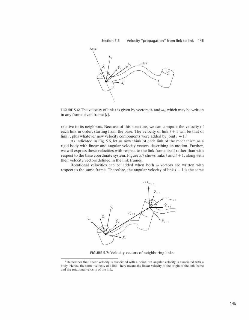
Section 5.6 Velocity ‘‘propagation’’ from link to link 145
Xi
YiZi
Axis i
Link iivi
i�i
FIGURE 5.6: The velocity of link i is given by vectors υi and ωi , which may be writtenin any frame, even frame {i}.
relative to its neighbors. Because of this structure, we can compute the velocity ofeach link in order, starting from the base. The velocity of link i + 1 will be that oflink i, plus whatever new velocity components were added by joint i + 1.2
As indicated in Fig. 5.6, let us now think of each link of the mechanism as arigid body with linear and angular velocity vectors describing its motion. Further,we will express these velocities with respect to the link frame itself rather than withrespect to the base coordinate system. Figure 5.7 shows links i and i + 1, along withtheir velocity vectors defined in the link frames.
Rotational velocities can be added when both ω vectors are written withrespect to the same frame. Therefore, the angular velocity of link i + 1 is the same
Xi
iPi � 1
Zi � 1
Xi � 1
Yi � 1
i � 1�i � 1
i � 1�i � 1
Yi
Zii�i
i�i
FIGURE 5.7: Velocity vectors of neighboring links.
2Remember that linear velocity is associated with a point, but angular velocity is associated with abody. Hence, the term ‘‘velocity of a link’’ here means the linear velocity of the origin of the link frameand the rotational velocity of the link.
145

146 Chapter 5 Jacobians: velocities and static forces
as that of link i plus a new component caused by rotational velocity at joint i + 1.This can be written in terms of frame {i} as
iωi+1 = iωi + i
i+1R θi+1
i+1Zi+1. (5.43)
Note that
θi+1i+1Zi+1 = i+1
00
θi+1
. (5.44)
We have made use of the rotation matrix relating frames {i} and {i + 1} in order torepresent the added rotational component due to motion at the joint in frame {i}.The rotation matrix rotates the axis of rotation of joint i + 1 into its description inframe {i}, so that the two components of angular velocity can be added.
By premultiplying both sides of (5.43) by i+1iR we can find the description of
the angular velocity of link i + 1 with respect to frame {i + 1}:
i+1ωi+1 = i+1iR iωi + θi+1
i+1Zi+1. (5.45)
The linear velocity of the origin of frame {i+1} is the same as that of the originof frame {i} plus a new component caused by rotational velocity of link i. This isexactly the situation described by (5.13), with one term vanishing because iPi+1 isconstant in frame {i}. Therefore, we have
iυi+1 = iυi + iωi × iPi+1. (5.46)
Premultiplying both sides by i+1iR, we compute
i+1υi+1 = i+1iR(iυi + iωi × iPi+1). (5.47)
Equations (5.45) and (5.47) are perhaps the most important results of this chapter.The corresponding relationships for the case that joint i + 1 is prismatic are
i+1ωi+1 = i+1iR iωi,
i+1υi+1 = i+1iR(iυi + iωi × iPi+1) + di+1
i+1Zi+1. (5.48)
Applying these equations successively from link to link, we can compute NωN andNυN , the rotational and linear velocities of the last link. Note that the resultingvelocities are expressed in terms of frame {N}. This turns out to be useful, as we willsee later. If the velocities are desired in terms of the base coordinate system, theycan be rotated into base coordinates by multiplication with 0
NR.
EXAMPLE 5.3
A two-link manipulator with rotational joints is shown in Fig. 5.8. Calculate thevelocity of the tip of the arm as a function of joint rates. Give the answer in twoforms—in terms of frame {3} and also in terms of frame {0}.
Frame {3} has been attached at the end of the manipulator, as shown in Fig. 5.9,and we wish to find the velocity of the origin of this frame expressed in frame {3}.As a second part of the problem, we will express these velocities in frame {0} as
146
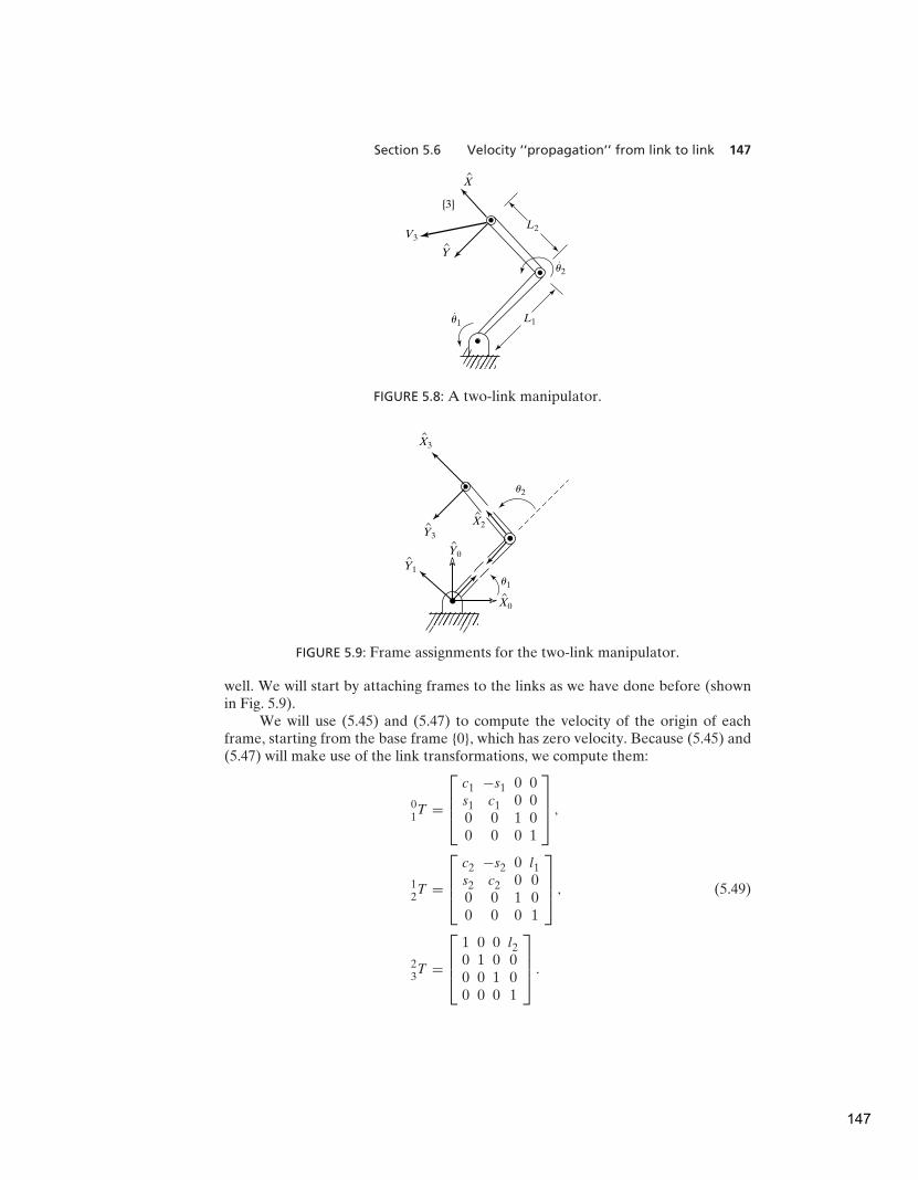
Section 5.6 Velocity ‘‘propagation’’ from link to link 147
{3}
L2V3
L1
u2·
u1·
X
Y
FIGURE 5.8: A two-link manipulator.
u2
u1
X3
X2
X0
Y3
Y0
Y1
FIGURE 5.9: Frame assignments for the two-link manipulator.
well. We will start by attaching frames to the links as we have done before (shownin Fig. 5.9).
We will use (5.45) and (5.47) to compute the velocity of the origin of eachframe, starting from the base frame {0}, which has zero velocity. Because (5.45) and(5.47) will make use of the link transformations, we compute them:
01T =
c1 −s1 0 0s1 c1 0 00 0 1 00 0 0 1
,
12T =
c2 −s2 0 l1s2 c2 0 00 0 1 00 0 0 1
, (5.49)
23T =
1 0 0 l20 1 0 00 0 1 00 0 0 1
.
147

148 Chapter 5 Jacobians: velocities and static forces
Note that these correspond to the manipulator of Example 3.3 with joint 3 perma-nently fixed at zero degrees. The final transformation between frames {2} and {3}
need not be cast as a standard link transformation (though it might be helpful to doso). Then, using (5.45) and (5.47) sequentially from link to link, we calculate
1ω1 =
00θ1
, (5.50)
1υ1 =
000
, (5.51)
2ω2 =
00
θ1 + θ2
, (5.52)
2υ2 =
c2 s2 0−s2 c2 0
0 0 1
0l1θ1
0
=
l1s2θ1l1c2θ1
0
, (5.53)
3ω3 = 2ω2, (5.54)
3υ3 =
l1s2θ1l1c2θ1 + l2(θ1 + θ2)
0
. (5.55)
Equation (5.55) is the answer. Also, the rotational velocity of frame {3} is found in(5.54).
To find these velocities with respect to the nonmoving base frame, we rotatethem with the rotation matrix 0
3R, which is
03R = 0
1R 1
2R 2
3R =
c12 −s12 0s12 c12 00 0 1
. (5.56)
This rotation yields
0υ3 =
−l1s1θ1 − l2s12(θ1 + θ2)
l1c1θ1 + l2c12(θ1 + θ2)
0
. (5.57)
It is important to point out the two distinct uses for (5.45) and (5.47). First,they can be used as a means of deriving analytical expressions, as in Example 5.3above. Here, we manipulate the symbolic equations until we arrive at a form suchas (5.55), which will be evaluated with a computer in some application. Second,they can be used directly to compute (5.45) and (5.47) as they are written. Theycan easily be written as a subroutine, which is then applied iteratively to computelink velocities. As such, they could be used for any manipulator, without the needof deriving the equations for a particular manipulator. However, the computation
148
Section 5.7 Jacobians 149
then yields a numeric result with the structure of the equations hidden. We are ofteninterested in the structure of an analytic result such as (5.55). Also, if we botherto do the work (that is, (5.50) through (5.57)), we generally will find that there arefewer computations left for the computer to perform in the final application.
5.7 JACOBIANS
The Jacobian is a multidimensional form of the derivative. Suppose, for example,that we have six functions, each of which is a function of six independent variables:
y1 = f1(x1, x2, x3, x4, x5, x6),
y2 = f2(x1, x2, x3, x4, x5, x6),
... (5.58)
y6 = f6(x1, x2, x3, x4, x5, x6).
We could also use vector notation to write these equations:
Y = F(X). (5.59)
Now, if we wish to calculate the differentials of yi as a function of differentials of xj ,we simply use the chain rule to calculate, and we get
δy1 =∂f1
∂x1
δx1 +∂f1
∂x2
δx2 + · · · +∂f1
∂x6
δx6,
δy2 =∂f2
∂x1
δx1 +∂f2
∂x2
δx2 + · · · +∂f2
∂x6
δx6,
... (5.60)
δy6 =∂f6
∂x1
δx1 +∂f6
∂x2
δx2 + · · · +∂f6
∂x6
δx6,
which again might be written more simply in vector notation:
δY =∂F
∂XδX. (5.61)
The 6 × 6 matrix of partial derivatives in (5.61) is what we call the Jacobian, J . Notethat, if the functions f1(X) through f6(X) are nonlinear, then the partial derivativesare a function of the xi , so, we can use the notation
δY = J (X)δX. (5.62)
By dividing both sides by the differential time element, we can think of the Jacobianas mapping velocities in X to those in Y :
Y = J (X)X. (5.63)
At any particular instant, X has a certain value, and J (X) is a linear transforma-tion. At each new time instant, X has changed, and therefore, so has the lineartransformation. Jacobians are time-varying linear transformations.
149
150 Chapter 5 Jacobians: velocities and static forces
In the field of robotics, we generally use Jacobians that relate joint velocitiesto Cartesian velocities of the tip of the arm—for example,
0ν = 0J (�)�, (5.64)
where� is the vector of joint angles of the manipulator and ν is a vector of Cartesianvelocities. In (5.64), we have added a leading superscript to our Jacobian notation toindicate in which frame the resulting Cartesian velocity is expressed. Sometimes thissuperscript is omitted when the frame is obvious or when it is unimportant to thedevelopment. Note that, for any given configuration of the manipulator, joint ratesare related to velocity of the tip in a linear fashion, yet this is only an instantaneousrelationship—in the next instant, the Jacobian has changed slightly. For the generalcase of a six-jointed robot, the Jacobian is 6 × 6, � is 6 × 1, and 0ν is 6 × 1. This 6 × 1Cartesian velocity vector is the 3 × 1 linear velocity vector and the 3 × 1 rotationalvelocity vector stacked together:
0ν =
[
0υ0ω
]
. (5.65)
Jacobians of any dimension (including nonsquare) can be defined. The numberof rows equals the number of degrees of freedom in the Cartesian space beingconsidered. The number of columns in a Jacobian is equal to the number of jointsof the manipulator. In dealing with a planar arm, for example, there is no reasonfor the Jacobian to have more than three rows, although, for redundant planarmanipulators, there could be arbitrarily many columns (one for each joint).
In the case of a two-link arm, we can write a 2 × 2 Jacobian that relatesjoint rates to end-effector velocity. From the result of Example 5.3, we can easilydetermine the Jacobian of our two-link arm. The Jacobian written in frame {3} isseen (from (5.55)) to be
3J (�) =
[
l1s2 0l1c2 + l2 l2
]
, (5.66)
and the Jacobian written in frame {0} is (from (5.57))
0J (�) =
[
−l1s1 − l2s12 −l2s12l1c1 + l2c12 l2c12
]
. (5.67)
Note that, in both cases, we have chosen to write a square matrix that relates jointrates to end-effector velocity. We could also consider a 3 × 2 Jacobian that wouldinclude the angular velocity of the end-effector.
Considering (5.58) through (5.62), which define the Jacobian, we see that theJacobian might also be found by directly differentiating the kinematic equationsof the mechanism. This is straightforward for linear velocity, but there is no 3 × 1orientation vector whose derivative is ω. Hence, we have introduced a method toderive the Jacobian by using successive application of (5.45) and (5.47). There areseveral other methods that can be used (see, for example, [4]), one of which will beintroduced shortly in Section 5.8. One reason for deriving Jacobians via the methodpresented is that it helps prepare us for material in Chapter 6, in which we will findthat similar techniques apply to calculating the dynamic equations of motion of amanipulator.
150

Section 5.8 Singularities 151
Changing a Jacobian’s frame of reference
Given a Jacobian written in frame {B}, that is,[
BυBω
]
= Bν = BJ (�)�, (5.68)
we might be interested in giving an expression for the Jacobian in another frame,{A}. First, note that a 6×1 Cartesian velocity vector given in {B} is described relativeto {A} by the transformation
[
AυAω
]
=
ABR 0
0 ABR
[
BυBω
]
. (5.69)
Hence, we can write
[
AυAω
]
=
ABR 0
0 ABR
BJ (�)�. (5.70)
Now it is clear that changing the frame of reference of a Jacobian is accom-plished by means of the following relationship:
AJ (�) =
ABR 0
0 ABR
BJ (�). (5.71)
5.8 SINGULARITIES
Given that we have a linear transformation relating joint velocity to Cartesianvelocity, a reasonable question to ask is: Is this matrix invertible? That is, is itnonsingular? If the matrix is nonsingular, then we can invert it to calculate jointrates from given Cartesian velocities:
� = J−1(�)ν. (5.72)
This is an important relationship. For example, say that we wish the hand of therobot to move with a certain velocity vector in Cartesian space. Using (5.72), wecould calculate the necessary joint rates at each instant along the path. The realquestion of invertibility is: Is the Jacobian invertible for all values of �? If not,where is it not invertible?
Most manipulators have values of � where the Jacobian becomes singular.Such locations are called singularities of the mechanism or singularities for short. Allmanipulators have singularities at the boundary of their workspace, and most haveloci of singularities inside their workspace. An in-depth study of the classification ofsingularities is beyond the scope of this book—for more information, see [5]. Forour purposes, and without giving rigorous definitions, we will class singularities intotwo categories:
1. Workspace-boundary singularities occur when the manipulator is fullystretched out or folded back on itself in such a way that the end-effectoris at or very near the boundary of the workspace.
151
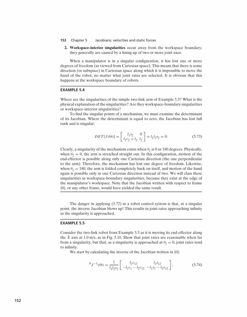
152 Chapter 5 Jacobians: velocities and static forces
2. Workspace-interior singularities occur away from the workspace boundary;they generally are caused by a lining up of two or more joint axes.
When a manipulator is in a singular configuration, it has lost one or moredegrees of freedom (as viewed from Cartesian space). This means that there is somedirection (or subspace) in Cartesian space along which it is impossible to move thehand of the robot, no matter what joint rates are selected. It is obvious that thishappens at the workspace boundary of robots.
EXAMPLE 5.4
Where are the singularities of the simple two-link arm of Example 5.3? What is thephysical explanation of the singularities? Are they workspace-boundary singularitiesor workspace-interior singularities?
To find the singular points of a mechanism, we must examine the determinantof its Jacobian. Where the determinant is equal to zero, the Jacobian has lost fullrank and is singular:
DET [J (�)] =
[
l1s2 0l1c2 + l2 l2
]
= l1l2s2 = 0. (5.73)
Clearly, a singularity of the mechanism exists when θ2 is 0 or 180 degrees. Physically,when θ2 = 0, the arm is stretched straight out. In this configuration, motion of theend-effector is possible along only one Cartesian direction (the one perpendicularto the arm). Therefore, the mechanism has lost one degree of freedom. Likewise,when θ2 = 180, the arm is folded completely back on itself, and motion of the handagain is possible only in one Cartesian direction instead of two. We will class thesesingularities as workspace-boundary singularities, because they exist at the edge ofthe manipulator’s workspace. Note that the Jacobian written with respect to frame{0}, or any other frame, would have yielded the same result.
The danger in applying (5.72) in a robot control system is that, at a singularpoint, the inverse Jacobian blows up! This results in joint rates approaching infinityas the singularity is approached.
EXAMPLE 5.5
Consider the two-link robot from Example 5.3 as it is moving its end-effector alongthe X axis at 1.0 m/s, as in Fig. 5.10. Show that joint rates are reasonable when farfrom a singularity, but that, as a singularity is approached at θ2 = 0, joint rates tendto infinity.
We start by calculating the inverse of the Jacobian written in {0}:
0J−1(�) =1
l1l2s2
[
l2c12 l2s12−l1c1 − l2c12 −l1s1 − l2s12
]
. (5.74)
152
Section 5.9 Static forces in manipulators 153
X3
X0
Y3
Y0
V3
�u2
u1
FIGURE 5.10: A two-link manipulator moving its tip at a constant linear velocity.
Then, using Eq. (5.74) for a velocity of 1 m/s in the X direction, we can calculatejoint rates as a function of manipulator configuration:
θ1 =c12
l1s2
, (5.75)
θ2 = −c1
l2s2
−c12
l1s2
.
Clearly, as the arm stretches out toward θ2 = 0, both joint rates go to infinity.
EXAMPLE 5.6
For the PUMA 560 manipulator, give two examples of singularities that can occur.There is singularity when θ3 is near −90.0 degrees. Calculation of the exact
value of θ3 is left as an exercise. (See Exercise 5.14.) In this situation, links 2 and3 are ‘‘stretched out,’’ just like the singular location of the two-link manipulator inExample 5.3. This is classed as a workspace-boundary singularity.
Whenever θ5 = 0.0 degrees, the manipulator is in a singular configuration. Inthis configuration, joint axes 4 and 6 line up—both of their actions would resultin the same end-effector motion, so it is as if a degree of freedom has been lost.Because this can occur interior to the workspace envelope, we will class it as aworkspace-interior singularity.
5.9 STATIC FORCES IN MANIPULATORS
The chainlike nature of a manipulator leads us quite naturally to consider how forcesand moments ‘‘propagate’’ from one link to the next. Typically, the robot is pushingon something in the environment with the chain’s free end (the end-effector) or isperhaps supporting a load at the hand. We wish to solve for the joint torques thatmust be acting to keep the system in static equilibrium.
In considering static forces in a manipulator, we first lock all the joints so thatthe manipulator becomes a structure. We then consider each link in this structureand write a force-moment balance relationship in terms of the link frames. Finally,
153

154 Chapter 5 Jacobians: velocities and static forces
we compute what static torque must be acting about the joint axis in order for themanipulator to be in static equilibrium. In this way, we solve for the set of jointtorques needed to support a static load acting at the end-effector.
In this section, we will not be considering the force on the links due to gravity(that will be left until chapter 6). The static forces and torques we are consideringat the joints are those caused by a static force or torque (or both) acting on the lastlink—for example, as when the manipulator has its end-effector in contact with theenvironment.
We define special symbols for the force and torque exerted by a neighbor link:fi = force exerted on link i by link i − 1,ni = torque exerted on link i by link i − 1.We will use our usual convention for assigning frames to links. Figure 5.11
shows the static forces and moments (excluding the gravity force) acting on link i.Summing the forces and setting them equal to zero, we have
ifi − ifi+1 = 0. (5.76)
Summing torques about the origin of frame {i}, we have
ini − ini+1 − iPi+1 × ifi+1 = 0. (5.77)
If we start with a description of the force and moment applied by the hand, wecan calculate the force and moment applied by each link, working from the last linkdown to the base (link 0). To do this, we formulate the force-moment expressions(5.76) and (5.77) such that they specify iterations from higher numbered links tolower numbered links. The result can be written as
ifi = ifi+1, (5.78)
ini = ini+1 + iPi+1 × ifi+1. (5.79)
In order to write these equations in terms of only forces and moments definedwithin their own link frames, we transform with the rotation matrix describing frame
iPi � 1 fi � 1
ni � 1
fi
ni
{i}
{i � 1}
FIGURE 5.11: Static force-moment balance for a single link.
154

Section 5.9 Static forces in manipulators 155
X3Y3
3F
t1
t2
FIGURE 5.12: A two-link manipulator applying a force at its tip.
{i + 1} relative to frame {i}. This leads to our most important result for static force‘‘propagation’’ from link to link:
ifi = i
i+1R i+1fi+1, (5.80)
ini = i
i+1R i+1ni+1 + iPi+1 × ifi . (5.81)
Finally, this important question arises: What torques are needed at the joints in orderto balance the reaction forces and moments acting on the links? All componentsof the force and moment vectors are resisted by the structure of the mechanismitself, except for the torque about the joint axis. Therefore, to find the joint torquerequired to maintain the static equilibrium, the dot product of the joint-axis vectorwith the moment vector acting on the link is computed:
τi = inTi
iZi . (5.82)
In the case that joint i is prismatic, we compute the joint actuator force as
τi = if T
i
iZi . (5.83)
Note that we are using the symbol τ even for a linear joint force.As a matter of convention, we generally define the positive direction of joint
torque as the direction which would tend to move the joint in the direction ofincreasing joint angle.
Equations (5.80) through (5.83) give us a means to compute the joint torquesneeded to apply any force or moment with the end-effector of a manipulator in thestatic case.
EXAMPLE 5.7
The two-link manipulator of Example 5.3 is applying a force vector 3F with itsend-effector. (Consider this force to be acting at the origin of {3}.) Find the requiredjoint torques as a function of configuration and of the applied force. (See Fig. 5.12.)
155

156 Chapter 5 Jacobians: velocities and static forces
We apply Eqs. (5.80) through (5.82), starting from the last link and goingtoward the base of the robot:
2f2 =
fx
fy
0
, (5.84)
2n2 = l2X2 ×
fx
fy
0
=
00
l2fy
, (5.85)
1f1 =
c2 −s2 0
s2 c2 0
0 0 1
fx
fy
0
=
c2fx − s2fy
s2fx + c2fy
0
, (5.86)
1n1 =
00
l2fy
+ l1X1 × 1f1 =
00
l1s2fx + l1c2fy + l2fy
. (5.87)
Therefore, we have
τ1 = l1s2fx + (l2 + l1c2)fy, (5.88)
τ2 = l2fy . (5.89)
This relationship can be written as a matrix operator:
τ =
[
l1s2 l2 + l1c2
0 l2
] [
fx
fy
]
. (5.90)
It is not a coincidence that this matrix is the transpose of the Jacobian that we foundin (5.66)!
5.10 JACOBIANS IN THE FORCE DOMAIN
We have found joint torques that will exactly balance forces at the hand in the staticsituation. When forces act on a mechanism, work (in the technical sense) is doneif the mechanism moves through a displacement. Work is defined as a force actingthrough a distance and is a scalar with units of energy. The principle of virtual workallows us to make certain statements about the static case by allowing the amount ofthis displacement to go to an infinitesimal. Work has the units of energy, so it mustbe the same measured in any set of generalized coordinates. Specifically, we canequate the work done in Cartesian terms with the work done in joint-space terms.In the multidimensional case, work is the dot product of a vector force or torqueand a vector displacement. Thus, we have
F · δχ = τ · δ�, (5.91)
where F is a 6 × 1 Cartesian force-moment vector acting at the end-effector, δχ isa 6 × 1 infinitesimal Cartesian displacement of the end-effector, τ is a 6 × 1 vector
156

Section 5.11 Cartesian transformation of velocities and static forces 157
of torques at the joints, and δ� is a 6 × 1 vector of infinitesimal joint displacements.Expression (5.91) can also be written as
FT δχ = τT δ�. (5.92)
The definition of the Jacobian is
δχ = Jδ�, (5.93)
so we may writeFT Jδθ = τT δ�, (5.94)
which must hold for all δ�; hence, we have
FT J = τT . (5.95)
Transposing both sides yields this result:
τ = J TF . (5.96)
Equation (5.96) verifies in general what we saw in the particular case of the two-linkmanipulator in Example 5.6: The Jacobian transpose maps Cartesian forces actingat the hand into equivalent joint torques. When the Jacobian is written with respectto frame {0}, then force vectors written in {0} can be transformed, as is made clearby the following notation:
τ = 0J T 0F . (5.97)
When the Jacobian loses full rank, there are certain directions in which the end-effector cannot exert static forces even if desired. That is, in (5.97), if the Jacobianis singular, F could be increased or decreased in certain directions (those definingthe null-space of the Jacobian [6]) without effect on the value calculated for τ . Thisalso means that, near singular configurations, mechanical advantage tends towardinfinity, such that, with small joint torques, large forces could be generated at theend-effector.3 Thus, singularities manifest themselves in the force domain as well asin the position domain.
Note that (5.97) is a very interesting relationship, in that it allows us to converta Cartesian quantity into a joint-space quantity without calculating any inversekinematic functions. We will make use of this when we consider the problem ofcontrol in later chapters.
5.11 CARTESIAN TRANSFORMATION OF VELOCITIES AND STATIC FORCES
We might wish to think in terms of 6 × 1 representations of general velocity of abody:
ν =
[
υ
ω
]
. (5.98)
Likewise, we could consider 6 × 1 representations of general force vectors,such as
F =
[
F
N
]
, (5.99)
3Consider a two-link planar manipulator nearly outstretched with the end-effector in contact with areaction surface. In this configuration, arbitrarily large forces could be exerted by ‘‘small’’ joint torques.
157
158 Chapter 5 Jacobians: velocities and static forces
where F is a 3 × 1 force vector and N is a 3 × 1 moment vector. It is then naturalto think of 6 × 6 transformations that map these quantities from one frame toanother. This is exactly what we have already done in considering the propagationof velocities and forces from link to link. Here, we write (5.45) and (5.47) in matrix-operator form to transform general velocity vectors in frame {A} to their descriptionin frame {B}.
The two frames involved here are rigidly connected, so θi+1, appearing in(5.45), is set to zero in deriving the relationship
[
BυBBωB
]
=
[
BAR −B
AR APBORG×
0 BAR
][
AυAAωA
]
, (5.100)
where the cross product is understood to be the matrix operator
P× =
0 −px pypx 0 −px
−py px 0
. (5.101)
Now, (5.100) relates velocities in one frame to those in another, so the 6×6 operatorwill be called a velocity transformation; we will use the symbol Tυ . In this case, it isa velocity transformation that maps velocities in {A} into velocities in {B}, so we usethe following notation to express (5.100) compactly:
BνB = B
ATυ
AνA. (5.102)
We can invert (5.100) in order to compute the description of velocity in terms of{A}, given the quantities in {B}:
[
AυAAωA
]
=
[
ABR APBORG × A
BR
0 ABR
] [
BυBBωB
]
, (5.103)
orAνA = A
BTυ
BνB . (5.104)
Note that these mappings of velocities from frame to frame depend on ABT (or its
inverse) and so must be interpreted as instantaneous results, unless the relationshipbetween the two frames is static. Similarly, from (5.80) and (5.81), we write the6 × 6 matrix that transforms general force vectors written in terms of {B} into theirdescription in frame {A}, namely,
[
AFAANA
]
=
[
ABR 0
APBORG × ABR A
BR
] [
BFBBNB
]
, (5.105)
which may be written compactly as
AFA = A
BTf
BFB , (5.106)
where Tf is used to denote a force-moment transformation.
158

Bibliography 159
Sensor
Sensor frame
Tool
ZWˆ
YWˆ
XWˆ
XTˆ ZT
ˆ
YTˆ
{W}
{T}
Wrist
FIGURE 5.13: Frames of interest with a force sensor.
Velocity and force transformations are similar to Jacobians in that they relatevelocities and forces in different coordinate systems. As with Jacobians, we have
A
BTf = A
BT T
υ, (5.107)
as can be verified by examining (5.105) and (5.103).
EXAMPLE 5.8
Figure 5.13 shows an end-effector holding a tool. Located at the point where theend-effector attaches to the manipulator is a force-sensing wrist. This is a devicethat can measure the forces and torques applied to it.
Consider the output of this sensor to be a 6 × 1 vector, SF , composed of threeforces and three torques expressed in the sensor frame, {S}. Our real interest is inknowing the forces and torques applied at the tip of the tool, T
F . Find the 6 × 6transformation that transforms the force-moment vector from {S} to the tool frame,{T }. The transform relating {T } to {S}, S
TT , is known. (Note that {S} here is the
sensor frame, not the station frame.)This is simply an application of (5.106). First, from S
TT , we calculate the inverse,
TST , which is composed of T
SR and T PSORG. Then we apply (5.106) to obtain
TFT = T
STf
SFS, (5.108)
where
T
STf =
[
TSR 0
T PSORG × TSR T
SR
]
. (5.109)
BIBLIOGRAPHY
[1] K. Hunt, Kinematic Geometry of Mechanisms, Oxford University Press, New York,1978.
[2] K.R. Symon, Mechanics, 3rd edition, Addison-Wesley, Reading, MA, 1971.
159
160 Chapter 5 Jacobians: velocities and static forces
[3] I. Shames, Engineering Mechanics, 2nd edition, Prentice-Hall, Englewood Cliffs, NJ,1967.
[4] D. Orin and W. Schrader, ‘‘Efficient Jacobian Determination for RobotManipulators,’’ in Robotics Research: The First International Symposium, M. Bradyand R.P. Paul, Editors, MIT Press, Cambridge, MA, 1984.
[5] B. Gorla and M. Renaud, Robots Manipulateurs, Cepadues-Editions, Toulouse, 1984.
[6] B. Noble, Applied Linear Algebra, Prentice-Hall, Englewood Cliffs, NJ, 1969.
[7] J.K. Salisbury and J. Craig, ‘‘Articulated Hands: Kinematic and Force Control Issues,’’International Journal of Robotics Research, Vol. 1, No. 1, Spring 1982.
[8] C. Wampler, ‘‘Wrist Singularities: Theory and Practice,’’ in The Robotics Review 2,O. Khatib, J. Craig, and T. Lozano-Perez, Editors, MIT Press, Cambridge, MA, 1992.
[9] D.E. Whitney, ‘‘Resolved Motion Rate Control of Manipulators and Human Prosthe-ses,’’ IEEE Transactions on Man-Machine Systems, 1969.
EXERCISES
5.1 [10] Repeat Example 5.3, but using the Jacobian written in frame {0}. Are theresults the same as those of Example 5.3?
5.2 [25] Find the Jacobian of the manipulator with three degrees of freedom fromExercise 3 of Chapter 3. Write it in terms of a frame {4} located at the tip of thehand and having the same orientation as frame {3}.
5.3 [35] Find the Jacobian of the manipulator with three degrees of freedom fromExercise 3 of Chapter 3. Write it in terms of a frame {4} located at the tip of thehand and having the same orientation as frame {3}. Derive the Jacobian in threedifferent ways: velocity propagation from base to tip, static force propagationfrom tip to base, and by direct differentiation of the kinematic equations.
5.4 [8] Prove that singularities in the force domain exist at the same configurations assingularities in the position domain.
5.5 [39] Calculate the Jacobian of the PUMA 560 in frame {6}.5.6 [47] Is it true that any mechanism with three revolute joints and nonzero link
lengths must have a locus of singular points interior to its workspace?5.7 [7] Sketch a figure of a mechanism with three degrees of freedom whose linear
velocity Jacobian is the 3 × 3 identity matrix over all configurations of themanipulator. Describe the kinematics in a sentence or two.
5.8 [18] General mechanisms sometimes have certain configurations, called ‘‘isotropicpoints,’’ where the columns of the Jacobian become orthogonal and of equalmagnitude [7]. For the two-link manipulator of Example 5.3, find out if anyisotropic points exist. Hint: Is there a requirement on l1 and l2?
5.9 [50] Find the conditions necessary for isotropic points to exist in a generalmanipulator with six degrees of freedom. (See Exercise 5.8.)
5.10 [7] For the two-link manipulator of Example 5.2, give the transformation thatwould map joint torques into a 2 × 1 force vector, 3F , at the hand.
5.11 [14] Given
A
BT =
0.866 −0.500 0.000 10.00.500 0.866 0.000 0.00.000 0.000 1.000 5.0
0 0 0 1
,
160

Exercises 161
if the velocity vector at the origin of {A} is
Aν =
0.02.0
−3.01.4141.4140.0
,
find the 6 × 1 velocity vector with reference point the origin of {B}.5.12 [15] For the three-link manipulator of Exercise 3.3, give a set of joint angles for
which the manipulator is at a workspace-boundary singularity and another set ofangles for which the manipulator is at a workspace-interior singularity.
5.13 [9] A certain two-link manipulator has the following Jacobian:
0J (�) =
[
−l1s1 − l2s12 −l2s12
l1c1 + l2c12 l2c12
]
.
Ignoring gravity, what are the joint torques required in order that the manipulatorwill apply a static force vector 0F = 10X0?
5.14 [18] If the link parameter a3 of the PUMA 560 were zero, a workspace-boundarysingularity would occur when θ3 = −90.0◦. Give an expression for the value of θ3where the singularity occurs, and show that, if a3 were zero, the result would beθ3 = −90.0◦. Hint: In this configuration, a straight line passes through joint axes2 and 3 and the point where axes 4, 5, and 6 intersect.
5.15 [24] Give the 3 × 3 Jacobian that calculates linear velocity of the tool tip fromthe three joint rates for the manipulator of Example 3.4 in Chapter 3. Give theJacobian in frame {0}.
5.16 [20] A 3R manipulator has kinematics that correspond exactly to the set ofZ–Y–Z Euler angles (i.e., the forward kinematics are given by (2.72) with α = θ1,β = θ2, and γ = θ3). Give the Jacobian relating joint velocities to the angularvelocity of the final link.
5.17 [31] Imagine that, for a general 6-DOF robot, we have available 0Zi and 0Piorgfor all i—that is, we know the values for the unit Z vectors of each link frame interms of the base frame and we know the locations of the origins of all link framesin terms of the base frame. Let us also say that we are interested in the velocity ofthe tool point (fixed relative to link n) and that we know 0Ptool also. Now, for arevolute joint, the velocity of the tool tip due to the velocity of joint i is given by
0υi = θi0Zi × (0Ptool −
0Piorg) (5.110)
and the angular velocity of link n due to the velocity of this joint is given by
0ωi = θi0Zi . (5.111)
The total linear and angular velocity of the tool is given by the sum of the 0υiand 0ωi respectively. Give equations analogous to (5.110) and (5.111) for the caseof joint i prismatic, and write the 6 × 6 Jacobian matrix of an arbitrary 6-DOFmanipulator in terms of the Zi , Piorg , and Ptool .
5.18 [18] The kinematics of a 3R robot are given by
03T =
c1c23 −c1s23 s1 l1c1 + l2c1c2
s1c23 −s1s23 −c1 l1s1 + l2s1c2
s23 c23 0 l2s2
0 0 0 1
.
161

162 Chapter 5 Jacobians: velocities and static forces
Find 0J (�), which, when multiplied by the joint velocity vector, gives the linearvelocity of the origin of frame {3} relative to frame {0}.
5.19 [15] The position of the origin of link 2 for an RP manipulator is given by
0P2ORG =
a1c1 − d2s1
a1s1 + d2c1
0
.
Give the 2 × 2 Jacobian that relates the two joint rates to the linear velocity ofthe origin of frame {2}. Give a value of � where the device is at a singularity.
5.20 [20] Explain what might be meant by the statement: ‘‘An n-DOF manipulator at asingularity can be treated as a redundant manipulator in a space of dimensionalityn− 1.’’
PROGRAMMING EXERCISE (PART 5)
1. Two frames, {A} and {B}, are not moving relative to one another—that is, ABT is
constant. In the planar case, we define the velocity of frame {A} as
AνA =
AxAAyAAθA
.
Write a routine that, given ABT and AνA, computes BνB . Hint: This is the planar
analog of (5.100). Use a procedure heading something like (or equivalent C):
Procedure Veltrans (VAR brela: frame; VAR vrela, vrelb: vec3);
where ‘‘vrela’’ is the velocity relative to frame {A}, or AνA, and ‘‘vrelb’’ is theoutput of the routine (the velocity relative to frame {B}), or BνB .
2. Determine the 3 × 3 Jacobian of the three-link planar manipulator (from Exam-ple 3.3). In order to derive the Jacobian, you should use velocity-propagationanalysis (as in Example 5.2) or static-force analysis (as in Example 5.6). Hand inyour work showing how you derived the Jacobian.
Write a routine to compute the Jacobian in frame {3}—that is, 3J (�)—as afunction of the joint angles. Note that frame {3} is the standard link frame withorigin on the axis of joint 3. Use a procedure heading something like (or equivalentC):
Procedure Jacobian (VAR theta: vec3; Var Jac: mat33);
The manipulator data are l2 = l2 = 0.5 meters.
3. A tool frame and a station frame are defined as follows by the user for a certaintask (units are meters and degrees):
W
TT = [x y θ] = [0.1 0.2 30.0],
B
ST = [x y θ] = [0.0 0.0 0.0].
At a certain instant, the tool tip is at the position
S
TT = [x y θ] = [0.6 − 0.3 45.0].
162
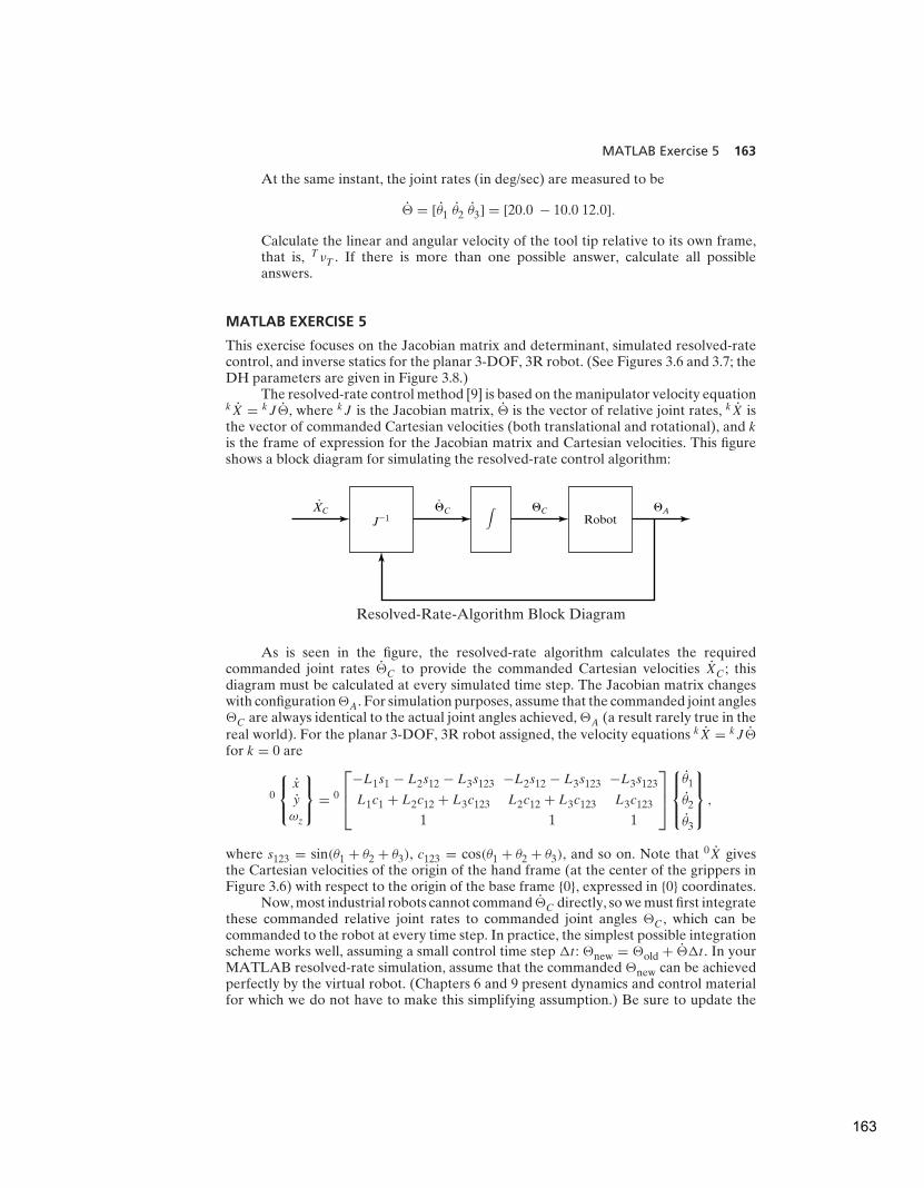
MATLAB Exercise 5 163
At the same instant, the joint rates (in deg/sec) are measured to be
� = [θ1 θ2 θ3] = [20.0 − 10.0 12.0].
Calculate the linear and angular velocity of the tool tip relative to its own frame,that is, T νT . If there is more than one possible answer, calculate all possibleanswers.
MATLAB EXERCISE 5
This exercise focuses on the Jacobian matrix and determinant, simulated resolved-ratecontrol, and inverse statics for the planar 3-DOF, 3R robot. (See Figures 3.6 and 3.7; theDH parameters are given in Figure 3.8.)
The resolved-rate control method [9] is based on the manipulator velocity equationkX = kJ �, where kJ is the Jacobian matrix, � is the vector of relative joint rates, kX isthe vector of commanded Cartesian velocities (both translational and rotational), and k
is the frame of expression for the Jacobian matrix and Cartesian velocities. This figureshows a block diagram for simulating the resolved-rate control algorithm:
RobotXC
J�1�C �C �A
K
Resolved-Rate-Algorithm Block Diagram
As is seen in the figure, the resolved-rate algorithm calculates the requiredcommanded joint rates �C to provide the commanded Cartesian velocities XC ; thisdiagram must be calculated at every simulated time step. The Jacobian matrix changeswith configuration�A. For simulation purposes, assume that the commanded joint angles�C are always identical to the actual joint angles achieved, �A (a result rarely true in thereal world). For the planar 3-DOF, 3R robot assigned, the velocity equations kX = kJ �
for k = 0 are
0
x
y
ωz
= 0
−L1s1 − L2s12 − L3s123 −L2s12 − L3s123 −L3s123
L1c1 + L2c12 + L3c123 L2c12 + L3c123 L3c123
1 1 1
θ1
θ2
θ3
,
where s123 = sin(θ1 + θ2 + θ3), c123 = cos(θ1 + θ2 + θ3), and so on. Note that 0X givesthe Cartesian velocities of the origin of the hand frame (at the center of the grippers inFigure 3.6) with respect to the origin of the base frame {0}, expressed in {0} coordinates.
Now, most industrial robots cannot command �C directly, so we must first integratethese commanded relative joint rates to commanded joint angles �C , which can becommanded to the robot at every time step. In practice, the simplest possible integrationscheme works well, assuming a small control time step �t : �new = �old + ��t . In yourMATLAB resolved-rate simulation, assume that the commanded �new can be achievedperfectly by the virtual robot. (Chapters 6 and 9 present dynamics and control materialfor which we do not have to make this simplifying assumption.) Be sure to update the
163

164 Chapter 5 Jacobians: velocities and static forces
Jacobian matrix with the new configuration �new before completing the resolved-ratecalculations for the next time step.
Develop a MATLAB program to calculate the Jacobian matrix and to simulateresolved-rate control for the planar 3R robot. Given the robot lengths L1 = 4, L2 = 3,and L3 = 2 (m); the initial joint angles � = {θ1 θ2 θ3}
T = {10◦
20◦
30◦}T , and the
constant commanded Cartesian rates 0{X} = {x y ωz}T = {0.2 −0.3 −0.2}T (m/s,
m/s, rad/s), simulate for exactly 5 sec, using time steps of exactly dt = 0.1 sec. Inthe same program loop, calculate the inverse-statics problem—that is, calculate thejoint torques T = {τ1 τ2 τ3}
T (Nm), given the constant commanded Cartesian wrench0{W } = {fx fy mz}
T = {1 2 3}T (N, N, Nm). Also, in the same loop, animate the robotto the screen during each time step, so that you can watch the simulated motion to verifythat it is correct.
a) For the specific numbers assigned, present five plots (each set on a separate graph,please):
1. the three active joint rates � = {θ1 θ2 θ3}T vs. time;
2. the three active joint angles � = {θ1 θ2 θ3}T vs. time;
3. the three Cartesian components of 0HT , X = {x y φ}T (rad is fine for φ so
that it will fit) vs. time;
4. the Jacobian matrix determinant |J | vs. time—comment on nearness tosingularities during the simulated resolved-rate motion;
5. the three active joint torques T = {τ1 τ2 τ3}T vs. time.
Carefully label (by hand is fine!) each component on each plot; also, label the axeswith names and units.
b) Check your Jacobian matrix results for the initial and final joint-angle sets bymeans of the Corke MATLAB Robotics Toolbox. Try function jacob0(). Caution:The toolbox Jacobian functions are for motion of {3} with respect to {0}, not for {H }
with respect to {0} as in the problem assignment. The preceding function gives theJacobian result in {0} coordinates; jacobn() would give results in {3} coordinates.
164

C H A P T E R 6
Manipulator dynamics
6.1 INTRODUCTION
6.2 ACCELERATION OF A RIGID BODY
6.3 MASS DISTRIBUTION
6.4 NEWTON’S EQUATION, EULER’S EQUATION
6.5 ITERATIVE NEWTON–EULER DYNAMIC FORMULATION
6.6 ITERATIVE VS. CLOSED FORM
6.7 AN EXAMPLE OF CLOSED-FORM DYNAMIC EQUATIONS
6.8 THE STRUCTURE OF A MANIPULATOR’S DYNAMIC EQUATIONS
6.9 LAGRANGIAN FORMULATION OF MANIPULATOR DYNAMICS
6.10 FORMULATING MANIPULATOR DYNAMICS IN CARTESIAN SPACE
6.11 INCLUSION OF NONRIGID BODY EFFECTS
6.12 DYNAMIC SIMULATION
6.13 COMPUTATIONAL CONSIDERATIONS
6.1 INTRODUCTION
Our study of manipulators so far has focused on kinematic considerations only.
We have studied static positions, static forces, and velocities; but we have never
considered the forces required to cause motion. In this chapter, we consider the
equations of motion for a manipulator—the way in which motion of the manipulator
arises from torques applied by the actuators or from external forces applied to the
manipulator.
Dynamics of mechanisms is a field in which many books have been written.
Indeed, one can spend years studying the field. Obviously, we cannot cover the
material in the completeness it deserves. However, certain formulations of the
dynamics problem seem particularly well suited to application to manipulators. In
particular, methods which make use of the serial-chain nature of manipulators are
natural candidates for our study.
There are two problems related to the dynamics of a manipulator that we wish
to solve. In the first problem, we are given a trajectory point, �, �, and �, and we
wish to find the required vector of joint torques, τ . This formulation of dynamics
is useful for the problem of controlling the manipulator (Chapter 10). The second
problem is to calculate how the mechanism will move under application of a set of
joint torques. That is, given a torque vector, τ , calculate the resulting motion of the
manipulator, �, �, and �. This is useful for simulating the manipulator.
From Chapter 6 of Introduction to Robotics: Mechanics and Control, Third Edition. John J. Craig.
Copyright © 2005 by Pearson Education, Inc. All rights reserved.
165
166 Chapter 6 Manipulator dynamics
6.2 ACCELERATION OF A RIGID BODY
We now extend our analysis of rigid-body motion to the case of accelerations. Atany instant, the linear and angular velocity vectors have derivatives that are calledthe linear and angular accelerations, respectively. That is,
B VQ =d
dt
BVQ = limt→o
BVQ(t +t)−BVQ(t)
t, (6.1)
and
A�B =d
dt
A�B = limt→o
A�B(t +t)−A�B(t)
t. (6.2)
As with velocities, when the reference frame of the differentiation is understood tobe some universal reference frame, {U}, we will use the notation
vA = U VAORG (6.3)
and
ωA = U �A. (6.4)
Linear acceleration
We start by restating (5.12), an important result from Chapter 5, which describesthe velocity of a vector BQ as seen from frame {A} when the origins are coincident:
AVQ = A
BR BVQ + A�B × A
BR BQ. (6.5)
The left-hand side of this equation describes how AQ is changing in time. So, becauseorigins are coincident, we could rewrite (6.5) as
d
dt(ABR BQ) = A
BR BVQ + A�B × A
BR BQ. (6.6)
This form of the equation will be useful when deriving the corresponding accelerationequation.
By differentiating (6.5), we can derive expressions for the acceleration of BQas viewed from {A} when the origins of {A} and {B} coincide:
AVQ =d
dt(ABR BVQ)+
A�B × A
BR BQ+ A�B ×
d
dt(ABR BQ). (6.7)
Now we apply (6.6) twice—once to the first term, and once to the last term. Theright-hand side of equation (6.7) becomes
ABR B VQ + A�B × A
BR BVQ + A�B × A
BR BQ
+ A�B × (ABR BVQ + A�B × A
BR BQ).
(6.8)
Combining two terms, we get
A
BR B VQ + 2A�B × A
BR BVQ + A�B × A
BR BQ+ A�B × (A�B × A
BR BQ). (6.9)
166
Section 6.3 Mass distribution 167
Finally, to generalize to the case in which the origins are not coincident, we add oneterm which gives the linear acceleration of the origin of {B}, resulting in the finalgeneral formula:
AVBORG + A
BR B VQ + 2A�B × A
BR BVQ + A�B × A
BR BQ (6.10)
+ A�B × (A�B × A
BR BQ).
A particular case that is worth pointing out is when BQ is constant, or
BVQ = B VQ = 0. (6.11)
In this case, (6.10) simplifies to
AVQ = AVBORG + A�B × (A�B × A
BR BQ)+ A�B × A
BR BQ. (6.12)
We will use this result in calculating the linear acceleration of the links of amanipulator with rotational joints. When a prismatic joint is present, the moregeneral form of (6.10) will be used.
Angular acceleration
Consider the case in which {B} is rotating relative to {A} with A�B and {C} is rotatingrelative to {B} with B�C . To calculate A�C , we sum the vectors in frame {A}:
A�C = A�B + A
BR B�C . (6.13)
By differentiating, we obtain
A�C = A�B +d
dt(ABR B�C). (6.14)
Now, applying (6.6) to the last term of (6.14), we get
A�C = A�B + A
BR B�C + A�B × A
BR B�C . (6.15)
We will use this result to calculate the angular acceleration of the links of amanipulator.
6.3 MASS DISTRIBUTION
In systems with a single degree of freedom, we often talk about the mass of a rigidbody. In the case of rotational motion about a single axis, the notion of the moment
of inertia is a familiar one. For a rigid body that is free to move in three dimensions,there are infinitely many possible rotation axes. In the case of rotation about anarbitrary axis, we need a complete way of characterizing the mass distribution of arigid body. Here, we introduce the inertia tensor, which, for our purposes, can bethought of as a generalization of the scalar moment of inertia of an object.
We shall now define a set of quantities that give information about thedistribution of mass of a rigid body relative to a reference frame. Figure 6.1 showsa rigid body with an attached frame. Inertia tensors can be defined relative to anyframe, but we will always consider the case of an inertia tensor defined for a frame
167
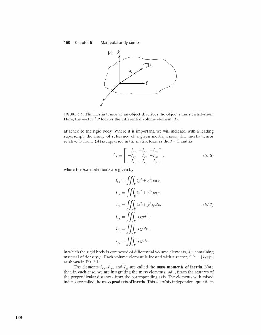
168 Chapter 6 Manipulator dynamics
{A}
AP
dv
Z^
X^
Y^
FIGURE 6.1: The inertia tensor of an object describes the object’s mass distribution.Here, the vector AP locates the differential volume element, dv.
attached to the rigid body. Where it is important, we will indicate, with a leadingsuperscript, the frame of reference of a given inertia tensor. The inertia tensorrelative to frame {A} is expressed in the matrix form as the 3 × 3 matrix
AI =
Ixx −Ixy −Ixz−Ixy Iyy −Iyz−Ixz −Iyz Izz
, (6.16)
where the scalar elements are given by
Ixx =
∫∫∫
V
(y2 + z2)ρdv,
Iyy =
∫∫∫
V
(x2 + z2)ρdv,
Izz =
∫∫∫
V
(x2 + y2)ρdv, (6.17)
Ixy =
∫∫∫
V
xyρdv,
Ixz =
∫∫∫
V
xzρdv,
Iyz =
∫∫∫
V
yzρdv,
in which the rigid body is composed of differential volume elements, dv, containingmaterial of density ρ. Each volume element is located with a vector, AP = [xyz]T ,as shown in Fig. 6.1.
The elements Ixx, Iyy , and Izz are called the mass moments of inertia. Notethat, in each case, we are integrating the mass elements, ρdv, times the squares ofthe perpendicular distances from the corresponding axis. The elements with mixedindices are called the mass products of inertia. This set of six independent quantities
168

Section 6.3 Mass distribution 169
will, for a given body, depend on the position and orientation of the frame in whichthey are defined. If we are free to choose the orientation of the reference frame, it ispossible to cause the products of inertia to be zero. The axes of the reference framewhen so aligned are called the principal axes and the corresponding mass momentsare the principal moments of inertia.
EXAMPLE 6.1
Find the inertia tensor for the rectangular body of uniform density ρ with respect tothe coordinate system shown in Fig. 6.2.
First, we compute Ixx . Using volume element dv = dx dy dz, we get
Ixx =
∫ h
0
∫ l
0
∫ ω
0(y2 + z2)ρ dx dy dz
=
∫ h
0
∫ l
0(y2 + z2)ωρdy dz (6.18)
=
∫ h
0
(
l3
3+ z2l
)
ωρdz
=
(
hl3ω
3+h3lω
3
)
ρ
=m
3(l2 + h2),
where m is the total mass of the body. Permuting the terms, we can get Iyy and Izzby inspection:
Iyy =m
3(ω2 + h2) (6.19)
andIzz =
m
3(l2 + ω2). (6.20)
{A}
l
h
w
X
Y
Z
FIGURE 6.2: A body of uniform density.
169

170 Chapter 6 Manipulator dynamics
We next compute Ixy :
Ixy =
∫ h
0
∫ l
0
∫ ω
0xyρ dx dy dz
=
∫ h
0
∫ l
0
ω2
2yρ dy dz (6.21)
=
∫ h
0
ω2l2
4ρdz
=m
4ωl.
Permuting the terms, we get
Ixz =m
4hω (6.22)
andIyz =
m
4hl. (6.23)
Hence, the inertia tensor for this object is
AI =
m3 (l
2 + h2) −m4 ωl −m
4 hω
−m4 ωl
m3 (ω
2 + h2) −m4 hl
−m4 hω −m
4 hlm3 (l
2 + ω2)
. (6.24)
As noted, the inertia tensor is a function of the location and orientation ofthe reference frame. A well-known result, the parallel-axis theorem, is one wayof computing how the inertia tensor changes under translations of the referencecoordinate system. The parallel-axis theorem relates the inertia tensor in a framewith origin at the center of mass to the inertia tensor with respect to anotherreference frame. Where {C} is located at the center of mass of the body, and {A} isan arbitrarily translated frame, the theorem can be stated [1] as
AIzz = CIzz +m(x2c
+ y2c),
AIxy = CIxy −mxcyc, (6.25)
where Pc = [xc, yc, zc]T locates the center of mass relative to {A}. The remaining
moments and products of inertia are computed from permutations of x,y, and z in(6.25). The theorem may be stated in vector–matrix form as
AI = CI +m[P TcPcI3 − PcP
T
c], (6.26)
where I3 is the 3 × 3 identity matrix.
EXAMPLE 6.2
Find the inertia tensor for the same solid body described for Example 6.1 when it isdescribed in a coordinate system with origin at the body’s center of mass.
170

Section 6.4 Newton’s equation, Euler’s equation 171
We can apply the parallel-axis theorem, (6.25), where
xcyczc
=1
2
ω
l
h
.
Next, we find
CIzz =m
12(ω2 + l2),
CIxy = 0. (6.27)
The other elements are found by symmetry. The resulting inertia tensor written inthe frame at the center of mass is
CI =
m12 (h
2 + l2) 0 0
0 m12 (ω
2 + h2) 0
0 0 m12 (l
2 + ω2)
. (6.28)
The result is diagonal, so frame {C} must represent the principal axes of this body.
Some additional facts about inertia tensors are as follows:
1. If two axes of the reference frame form a plane of symmetry for the massdistribution of the body, the products of inertia having as an index thecoordinate that is normal to the plane of symmetry will be zero.
2. Moments of inertia must always be positive. Products of inertia may haveeither sign.
3. The sum of the three moments of inertia is invariant under orientation changesin the reference frame.
4. The eigenvalues of an inertia tensor are the principal moments for the body.The associated eigenvectors are the principal axes.
Most manipulators have links whose geometry and composition are somewhatcomplex, so that the application of (6.17) is difficult in practice. A pragmatic optionis actually to measure rather than to calculate the moment of inertia of each link byusing a measuring device (e.g., an inertia pendulum).
6.4 NEWTON’S EQUATION, EULER’S EQUATION
We will consider each link of a manipulator as a rigid body. If we know thelocation of the center of mass and the inertia tensor of the link, then its massdistribution is completely characterized. In order to move the links, we mustaccelerate and decelerate them. The forces required for such motion are a functionof the acceleration desired and of the mass distribution of the links. Newton’sequation, along with its rotational analog, Euler’s equation, describes how forces,inertias, and accelerations relate.
171

172 Chapter 6 Manipulator dynamics
F
v�c
FIGURE 6.3: A force F acting at the center of mass of a body causes the body toaccelerate at vC .
Newton’s equation
Figure 6.3 shows a rigid body whose center of mass is accelerating with accelerationvC . In such a situation, the force, F , acting at the center of mass and causing thisacceleration is given by Newton’s equation
F = mvC, (6.29)
where m is the total mass of the body.
Euler’s equation
Figure 6.4 shows a rigid body rotating with angular velocity ω and with angularacceleration ω. In such a situation, the moment N , which must be acting on the bodyto cause this motion, is given by Euler’s equation
N = CI ω + ω × CIω, (6.30)
where CI is the inertia tensor of the body written in a frame, {C}, whose origin islocated at the center of mass.
v•v
N
FIGURE 6.4: A moment N is acting on a body, and the body is rotating with velocityω and accelerating at ω.
172
Section 6.5 Iterative Newton–Euler dynamic formulation 173
6.5 ITERATIVE NEWTON–EULER DYNAMIC FORMULATION
We now consider the problem of computing the torques that correspond to agiven trajectory of a manipulator. We assume we know the position, velocity, andacceleration of the joints, (�, �, �). With this knowledge, and with knowledge ofthe kinematics and the mass-distribution information of the robot, we can calculatethe joint torques required to cause this motion. The algorithm presented is basedupon the method published by Luh, Walker, and Paul in [2].
Outward iterations to compute velocities and accelerations
In order to compute inertial forces acting on the links, it is necessary to computethe rotational velocity and linear and rotational acceleration of the center of massof each link of the manipulator at any given instant. These computations will bedone in an iterative way, starting with link 1 and moving successively, link by link,outward to link n.
The ‘‘propagation’’ of rotational velocity from link to link was discussed inChapter 5 and is given (for joint i + 1 rotational) by
i+1ωi+1 = i+1iR iωi + θi+1
i+1Zi+1. (6.31)
From (6.15), we obtain the equation for transforming angular acceleration from onelink to the next:
i+1ωi+1 = i+1iR iωi +
i+1iR iωi × θi+1
i+1Zi+1 + θi+1i+1Zi+1. (6.32)
When joint i + 1 is prismatic, this simplifies to
i+1ωi+1 = i+1iR iωi . (6.33)
The linear acceleration of each link-frame origin is obtained by the application of(6.12):
i+1vi+1 = i+1iR[iωi ×
iPi+1 + iωi × (iωi ×
iPi+1)+i vi], (6.34)
For prismatic joint i + 1, (6.34) becomes (from (6.10))
i+1vi+1 = i+1iR(iωi ×
iPi+1 + iωi × (iωi ×
iPi+1)+i vi)
+ 2i+1ωi+1 × di+1i+1Zi+1 + di+1
i+1Zi+1. (6.35)
We also will need the linear acceleration of the center of mass of each link, whichalso can be found by applying (6.12):
i vCi= iωi ×
iPCi+ iωi × (
iωi +iPCi
)+ i vi, (6.36)
Here, we imagine a frame, {Ci}, attached to each link, having its origin located atthe center of mass of the link and having the same orientation as the link frame,{i}. Equation (6.36) doesn’t involve joint motion at all and so is valid for joint i + 1,regardless of whether it is revolute or prismatic.
Note that the application of the equations to link 1 is especially simple, because0ω0 = 0ω0 = 0.
173

174 Chapter 6 Manipulator dynamics
The force and torque acting on a link
Having computed the linear and angular accelerations of the mass center of eachlink, we can apply the Newton–Euler equations (Section 6.4) to compute the inertialforce and torque acting at the center of mass of each link. Thus we have
Fi = mvCi,
Ni = Ci I ωi + ωi ×Ci Iωi, (6.37)
where {Ci} has its origin at the center of mass of the link and has the same orientationas the link frame, {i}.
Inward iterations to compute forces and torques
Having computed the forces and torques acting on each link, we now need tocalculate the joint torques that will result in these net forces and torques beingapplied to each link.
We can do this by writing a force-balance and moment-balance equation basedon a free-body diagram of a typical link. (See Fig. 6.5.) Each link has forces andtorques exerted on it by its neighbors and in addition experiences an inertial forceand torque. In Chapter 5, we defined special symbols for the force and torqueexerted by a neighbor link, which we repeat here:
fi = force exerted on link i by link i − 1,ni = torque exerted on link i by link i − 1.
By summing the forces acting on link i, we arrive at the force-balancerelationship:
iFi = ifi −i
i+1Ri+1fi+1. (6.38)
By summing torques about the center of mass and setting them equal to zero,we arrive at the torque-balance equation:
iNi = ini −ini+1 + (−iPCi
)× ifi − (iPi+1 − iPCi
)× ifi+1. (6.39)
fi
Ni
Fi
fi � 1
ni � 1
ni
{i}
{i � 1 }
FIGURE 6.5: The force balance, including inertial forces, for a single manipulator link.
174
Section 6.5 Iterative Newton–Euler dynamic formulation 175
Using the result from the force-balance relation (6.38) and adding a few
rotation matrices, we can write (6.39) as
iNi = ini −i
i+1R i+1ni+1 − iPCi
× iFi −iPi+1 × i
i+1R i+1fi+1. (6.40)
Finally, we can rearrange the force and torque equations so that they appear as
iterative relationships from higher numbered neighbor to lower numbered neighbor:
ifi = i
i+1R i+1fi+1 + iFi, (6.41)
ini = iNi +i
i+1R i+1ni+1 + iPCi
× iFi +iPi+1 × i
i+1R i+1fi+1. (6.42)
These equations are evaluated link by link, starting from link n and working
inward toward the base of the robot. These inward force iterations are analogous
to the static force iterations introduced in Chapter 5, except that inertial forces and
torques are now considered at each link.As in the static case, the required joint torques are found by taking the Z
component of the torque applied by one link on its neighbor:
τi = inTi
iZi . (6.43)
For joint i prismatic, we use
τi = if Ti
iZi, (6.44)
where we have used the symbol τ for a linear actuator force.
Note that, for a robot moving in free space, N+1fN+1 and N+1nN+1 are set
equal to zero, and so the first application of the equations for link n is very simple.
If the robot is in contact with the environment, the forces and torques due to
this contact can be included in the force balance by having nonzero N+1fN+1 andN+1nN+1.
The iterative Newton–Euler dynamics algorithm
The complete algorithm for computing joint torques from the motion of the joints
is composed of two parts. First, link velocities and accelerations are iteratively
computed from link 1 out to link n and the Newton–Euler equations are applied
to each link. Second, forces and torques of interaction and joint actuator torques
are computed recursively from link n back to link 1. The equations are summarized
next for the case of all joints rotational:
175
176 Chapter 6 Manipulator dynamics
Outward iterations: i : 0 → 5
i+1ωi+1 = i+1iR iωi + θi+1
i+1Zi+1, (6.45)
i+1ωi+1 = i+1iR iωi +
i+1iR iωi × θi+1
i+1Zi+1 + θi+1i+1Zi+1, (6.46)
i+1vi+1 = i+1iR(iωi ×
iPi+1 + iωi × (iωi ×
iPi+1)+i vi), (6.47)
i+1vCi+1= i+1ωi+1 × i+1PCi+1
+i+1ωi+1 × (i+1ωi+1 × i+1PCi+1)+ i+1vi+1, (6.48)
i+1Fi+1 = mi+1i+1vCi+1
, (6.49)
i+1Ni+1 = Ci+1Ii+1i+1ωi+1 + i+1ωi+1 × Ci+1Ii+1
i+1ωi+1. (6.50)
Inward iterations: i : 6 → 1
ifi = i
i+1R i+1fi+1 + iFi, (6.51)
ini = iNi +i
i+1R i+1ni+1 + iPCi
× iFi
+iPi+1 × i
i+1R i+1fi+1, (6.52)
τi = inTi
iZi . (6.53)
Inclusion of gravity forces in the dynamics algorithm
The effect of gravity loading on the links can be included quite simply by setting0v0 = G, whereG has the magnitude of the gravity vector but points in the oppositedirection. This is equivalent to saying that the base of the robot is acceleratingupward with 1 g acceleration. This fictitious upward acceleration causes exactly thesame effect on the links as gravity would. So, with no extra computational expense,the gravity effect is calculated.
6.6 ITERATIVE VS. CLOSED FORM
Equations (6.46) through (6.53) give a computational scheme whereby, given thejoint positions, velocities, and accelerations, we can compute the required jointtorques. As with our development of equations to compute the Jacobian inChapter 5, these relations can be used in two ways: as a numerical computationalalgorithm, or as an algorithm used analytically to develop symbolic equations.
Use of the equations as a numerical computational algorithm is attractivebecause the equations apply to any robot. Once the inertia tensors, link masses, PCivectors, and i+1
iR matrices are specified for a particular manipulator, the equations
can be applied directly to compute the joint torques corresponding to any motion.However, we often are interested in obtaining better insight into the structure
of the equations. For example, what is the form of the gravity terms? How doesthe magnitude of the gravity effects compare with the magnitude of the inertialeffects? To investigate these and other questions, it is often useful to write closed-form dynamic equations. These equations can be derived by applying the recursive
176
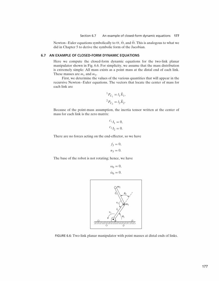
Section 6.7 An example of closed-form dynamic equations 177
Newton–Euler equations symbolically to�, �, and �. This is analogous to what wedid in Chapter 5 to derive the symbolic form of the Jacobian.
6.7 AN EXAMPLE OF CLOSED-FORM DYNAMIC EQUATIONS
Here we compute the closed-form dynamic equations for the two-link planarmanipulator shown in Fig. 6.6. For simplicity, we assume that the mass distributionis extremely simple: All mass exists as a point mass at the distal end of each link.These masses are m1 and m2.
First, we determine the values of the various quantities that will appear in therecursive Newton–Euler equations. The vectors that locate the center of mass foreach link are
1PC1= l1X1,
2PC2= l2X2.
Because of the point-mass assumption, the inertia tensor written at the center ofmass for each link is the zero matrix:
C1I1 = 0,
C2I2 = 0.
There are no forces acting on the end-effector, so we have
f3 = 0,
n3 = 0.
The base of the robot is not rotating; hence, we have
ω0 = 0,
ω0 = 0.
u1
u2
t1
t2
l1
l2
m1
m2
FIGURE 6.6: Two-link planar manipulator with point masses at distal ends of links.
177
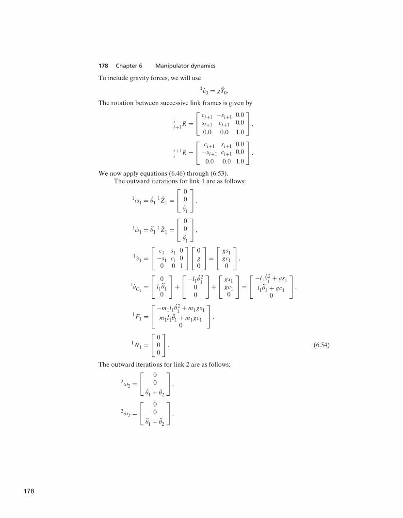
178 Chapter 6 Manipulator dynamics
To include gravity forces, we will use
0v0 = gY0.
The rotation between successive link frames is given by
i
i+1R =
ci+1 −si+1 0.0si+1 ci+1 0.0
0.0 0.0 1.0
,
i+1iR =
ci+1 si+1 0.0−si+1 ci+1 0.0
0.0 0.0 1.0
.
We now apply equations (6.46) through (6.53).The outward iterations for link 1 are as follows:
1ω1 = θ11Z1 =
00
θ1
,
1ω1 = θ11Z1 =
00
θ1
,
1v1 =
c1 s1 0−s1 c1 0
0 0 1
0g
0
=
gs1gc10
,
1vC1=
0l1θ1
0
+
−l1θ21
00
+
gs1gc10
=
−l1θ21
+ gs1
l1θ1 + gc10
,
1F1 =
−m1l1θ21
+m1gs1
m1l1θ1 +m1gc10
,
1N1 =
000
. (6.54)
The outward iterations for link 2 are as follows:
2ω2 =
00
θ1 + θ2
,
2ω2 =
00
θ1 + θ2
,
178
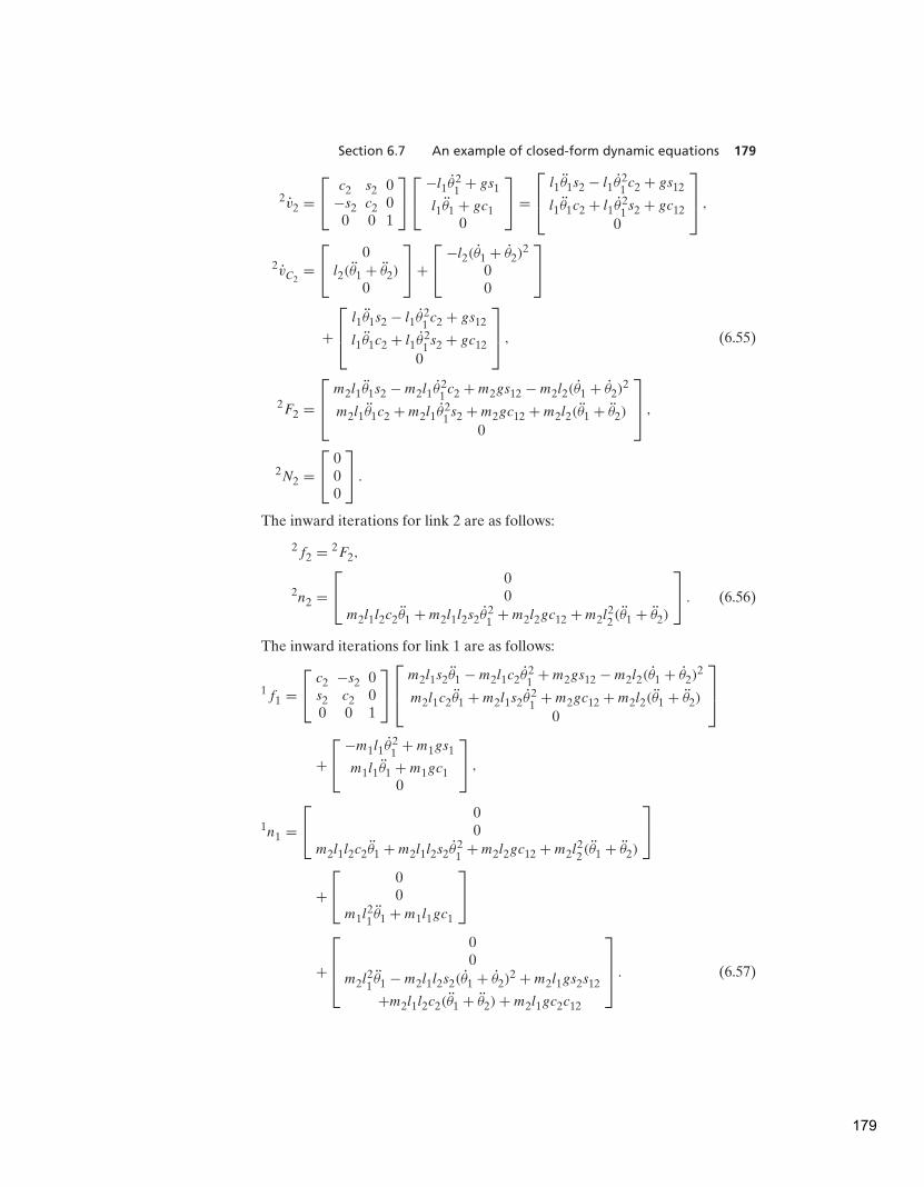
Section 6.7 An example of closed-form dynamic equations 179
2v2 =
c2 s2 0−s2 c2 0
0 0 1
−l1θ21
+ gs1
l1θ1 + gc10
=
l1θ1s2 − l1θ21c2 + gs12
l1θ1c2 + l1θ21s2 + gc12
0
,
2vC2=
0l2(θ1 + θ2)
0
+
−l2(θ1 + θ2)2
00
+
l1θ1s2 − l1θ21c2 + gs12
l1θ1c2 + l1θ21s2 + gc12
0
, (6.55)
2F2 =
m2l1θ1s2 −m2l1θ21c2 +m2gs12 −m2l2(θ1 + θ2)
2
m2l1θ1c2 +m2l1θ21s2 +m2gc12 +m2l2(θ1 + θ2)
0
,
2N2 =
000
.
The inward iterations for link 2 are as follows:
2f2 = 2F2,
2n2 =
00
m2l1l2c2θ1 +m2l1l2s2θ21
+m2l2gc12 +m2l22(θ1 + θ2)
. (6.56)
The inward iterations for link 1 are as follows:
1f1 =
c2 −s2 0s2 c2 00 0 1
m2l1s2θ1 −m2l1c2θ21
+m2gs12 −m2l2(θ1 + θ2)2
m2l1c2θ1 +m2l1s2θ21
+m2gc12 +m2l2(θ1 + θ2)
0
+
−m1l1θ21
+m1gs1
m1l1θ1 +m1gc10
,
1n1 =
00
m2l1l2c2θ1 +m2l1l2s2θ21
+m2l2gc12 +m2l22(θ1 + θ2)
+
00
m1l21θ1 +m1l1gc1
+
00
m2l21θ1 −m2l1l2s2(θ1 + θ2)
2 +m2l1gs2s12
+m2l1l2c2(θ1 + θ2)+m2l1gc2c12
. (6.57)
179
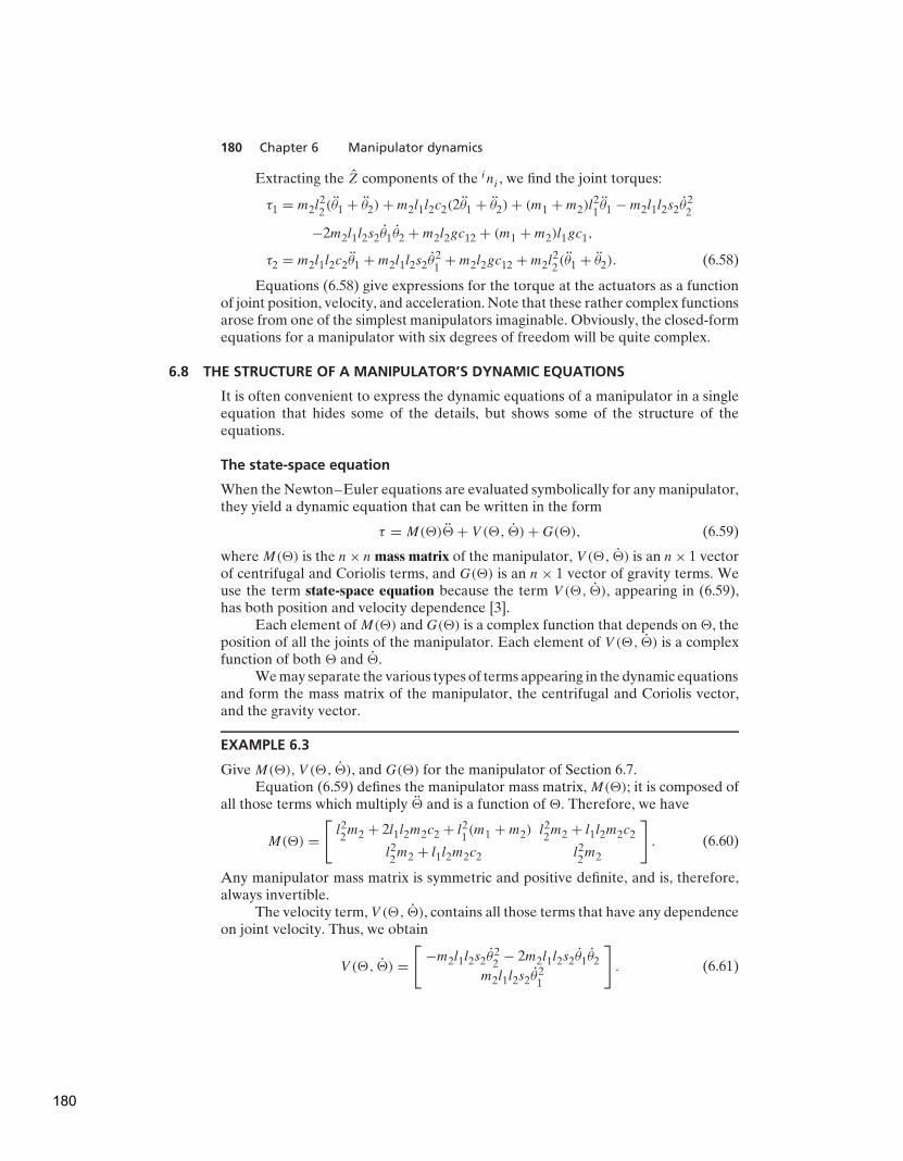
180 Chapter 6 Manipulator dynamics
Extracting the Z components of the ini , we find the joint torques:
τ1 = m2l22(θ1 + θ2)+m2l1l2c2(2θ1 + θ2)+ (m1 +m2)l
21θ1 −m2l1l2s2θ
22
−2m2l1l2s2θ1θ2 +m2l2gc12 + (m1 +m2)l1gc1,
τ2 = m2l1l2c2θ1 +m2l1l2s2θ21
+m2l2gc12 +m2l22(θ1 + θ2). (6.58)
Equations (6.58) give expressions for the torque at the actuators as a functionof joint position, velocity, and acceleration. Note that these rather complex functionsarose from one of the simplest manipulators imaginable. Obviously, the closed-formequations for a manipulator with six degrees of freedom will be quite complex.
6.8 THE STRUCTURE OF A MANIPULATOR’S DYNAMIC EQUATIONS
It is often convenient to express the dynamic equations of a manipulator in a singleequation that hides some of the details, but shows some of the structure of theequations.
The state-space equation
When the Newton–Euler equations are evaluated symbolically for any manipulator,they yield a dynamic equation that can be written in the form
τ = M(�)�+ V (�, �)+G(�), (6.59)
whereM(�) is the n× nmass matrix of the manipulator, V (�, �) is an n× 1 vectorof centrifugal and Coriolis terms, and G(�) is an n× 1 vector of gravity terms. Weuse the term state-space equation because the term V (�, �), appearing in (6.59),has both position and velocity dependence [3].
Each element ofM(�) andG(�) is a complex function that depends on�, theposition of all the joints of the manipulator. Each element of V (�, �) is a complexfunction of both � and �.
We may separate the various types of terms appearing in the dynamic equationsand form the mass matrix of the manipulator, the centrifugal and Coriolis vector,and the gravity vector.
EXAMPLE 6.3
GiveM(�), V (�, �), and G(�) for the manipulator of Section 6.7.Equation (6.59) defines the manipulator mass matrix,M(�); it is composed of
all those terms which multiply � and is a function of �. Therefore, we have
M(�) =
[
l22m2 + 2l1l2m2c2 + l2
1(m1 +m2) l
22m2 + l1l2m2c2
l22m2 + l1l2m2c2 l2
2m2
]
. (6.60)
Any manipulator mass matrix is symmetric and positive definite, and is, therefore,always invertible.
The velocity term, V (�, �), contains all those terms that have any dependenceon joint velocity. Thus, we obtain
V (�, �) =
[
−m2l1l2s2θ22
− 2m2l1l2s2θ1θ2
m2l1l2s2θ21
]
. (6.61)
180

Section 6.8 The structure of a manipulator’s dynamic equations 181
A term like −m2l1l2s2θ22
is caused by a centrifugal force, and is recognized as such
because it depends on the square of a joint velocity. A term such as −2m2l1l2s2θ1θ2is caused by a Coriolis force and will always contain the product of two differentjoint velocities.
The gravity term, G(�), contains all those terms in which the gravitationalconstant, g, appears. Therefore, we have
G(�) =
[
m2l2gc12 + (m1 +m2)l1gc1m2l2gc12
]
. (6.62)
Note that the gravity term depends only on � and not on its derivatives.
The configuration-space equation
By writing the velocity-dependent term, V (�, �), in a different form, we can writethe dynamic equations as
τ = M(�)�+ B(�)[��] + C(�)[�2] +G(�), (6.63)
where B(�) is a matrix of dimensions n × n(n − 1)/2 of Coriolis coefficients, [��]
is an n(n− 1)/2 × 1 vector of joint velocity products given by
[��] = [θ1θ2 θ1θ3 . . . θn−1θn]T , (6.64)
C(�) is an n× n matrix of centrifugal coefficients, and [�2] is an n× 1 vector givenby
[θ21θ2
2. . . θ2
n]T . (6.65)
We will call (6.63) the configuration-space equation, because the matrices arefunctions only of manipulator position [3].
In this form of the dynamic equations, the complexity of the computation isseen to be in the form of computing various parameters which are a function of onlythe manipulator position, �. This is important in applications (such as computercontrol of a manipulator) in which the dynamic equations must be updated asthe manipulator moves. (Equation (6.63) gives a form in which parameters are afunction of joint position only and can be updated at a rate related to how fast themanipulator is changing configuration.) We will consider this form again with regardto the problem of manipulator control in Chapter 10.
EXAMPLE 6.4
Give B(�) and C(�) (from (6.63)) for the manipulator of Section 6.7.For this simple two-link manipulator, we have
[��] = [θ1θ2],
[�2] =
[
θ21
θ22
]
. (6.66)
181

182 Chapter 6 Manipulator dynamics
So we see that
B(�) =
[
−2m2l1l2s2
0
]
(6.67)
and
C(�) =
[
0 −m2l1l2s2
m2l1l2s2 0
]
. (6.68)
6.9 LAGRANGIAN FORMULATION OF MANIPULATOR DYNAMICS
The Newton–Euler approach is based on the elementary dynamic formulas (6.29)and (6.30) and on an analysis of forces and moments of constraint acting betweenthe links. As an alternative to the Newton–Euler method, in this section webriefly introduce the Lagrangian dynamic formulation. Whereas the Newton–Eulerformulation might be said to be a ‘‘force balance’’ approach to dynamics, theLagrangian formulation is an ‘‘energy-based’’ approach to dynamics. Of course, forthe same manipulator, both will give the same equations of motion. Our statementof Lagrangian dynamics will be brief and somewhat specialized to the case of aserial-chain mechanical manipulator with rigid links. For a more complete andgeneral reference, see [4].
We start by developing an expression for the kinetic energy of a manipulator.The kinetic energy of the ith link, ki , can be expressed as
ki = 12miv
T
CivCi
+ 12iωTi
Ci Iiiωi, (6.69)
where the first term is kinetic energy due to linear velocity of the link’s centerof mass and the second term is kinetic energy due to angular velocity of the link.The total kinetic energy of the manipulator is the sum of the kinetic energy in theindividual links—that is,
k =
n∑
i=1
ki . (6.70)
The vCi and iωi in (6.69) are functions of � and �, so we see that the kinetic energy
of a manipulator can be described by a scalar formula as a function of joint positionand velocity, k(�, �). In fact, the kinetic energy of a manipulator is given by
k(�, �) = 12�
TM(�)�, (6.71)
whereM(�) is the n× nmanipulator mass matrix already introduced in Section 6.8.An expression of the form of (6.71) is known as a quadratic form [5], since whenexpanded out, the resulting scalar equation is composed solely of terms whosedependence on the θi is quadratic. Further, because the total kinetic energy mustalways be positive, the manipulator mass matrix must be a so-called positive definitematrix. Positive definite matrices are those having the property that their quadraticform is always a positive scalar. Equation (6.71) can be seen to be analogous to thefamiliar expression for the kinetic energy of a point mass:
k = 12mv
2. (6.72)
182

Section 6.9 Lagrangian formulation of manipulator dynamics 183
The fact that a manipulator mass matrix must be positive definite is analogous tothe fact that a scalar mass is always a positive number.
The potential energy of the ith link, ui , can be expressed as
ui = −mi0gT 0PCi
+ urefi, (6.73)
where 0g is the 3 × 1 gravity vector, 0PCiis the vector locating the center of mass of
the ith link, and urefi is a constant chosen so that the minimum value of ui is zero.1
The total potential energy stored in the manipulator is the sum of the potentialenergy in the individual links—that is,
u =
n∑
i=1
ui . (6.74)
Because the 0PCiin (6.73) are functions of �, we see that the potential energy
of a manipulator can be described by a scalar formula as a function of joint position,u(�).
The Lagrangian dynamic formulation provides a means of deriving the equa-tions of motion from a scalar function called the Lagrangian, which is defined as thedifference between the kinetic and potential energy of a mechanical system. In ournotation, the Lagrangian of a manipulator is
L(�, �) = k(�, �)− u(�). (6.75)
The equations of motion for the manipulator are then given by
d
dt
∂L
∂�−∂L
∂�= τ, (6.76)
where τ is the n × 1 vector of actuator torques. In the case of a manipulator, thisequation becomes
d
dt
∂k
∂�−∂k
∂�+∂u
∂�= τ, (6.77)
where the arguments of k(·) and u(·) have been dropped for brevity.
EXAMPLE 6.5
The links of an RP manipulator, shown in Fig. 6.7, have inertia tensors
C1I1 =
Ixx1 0 00 Iyy1 0
0 0 Izz1
,
C2I2 =
Ixx2 0 00 Iyy2 0
0 0 Izz2
, (6.78)
1Actually, only the partial derivative of the potential energy with respect to � will appear in thedynamics, so this constant is arbitrary. This corresponds to defining the potential energy relative to anarbitrary zero reference height.
183

184 Chapter 6 Manipulator dynamics
l1
m1
u1
m2
g
d2
FIGURE 6.7: The RP manipulator of Example 6.5.
and total mass m1 and m2. As shown in Fig. 6.7, the center of mass of link 1 islocated at a distance l1 from the joint-1 axis, and the center of mass of link 2 is at thevariable distance d2 from the joint-1 axis. Use Lagrangian dynamics to determinethe equation of motion for this manipulator.
Using (6.69), we write the kinetic energy of link 1 as
k1 = 12m1l
21θ2
1+ 1
2Izz1 θ21
(6.79)
and the kinetic energy of link 2 as
k2 = 12m2(d
22θ2
1+ d2
2)+ 1
2Izz2 θ21. (6.80)
Hence, the total kinetic energy is given by
k(�, �) = 12 (m1l
21
+ Izz1 + Izz2 +m2d22)θ2
1+ 1
2m2d22. (6.81)
Using (6.73), we write the potential energy of link 1 as
u1 = m1l1g sin(θ1)+m1l1g (6.82)
and the potential energy of link 2 as
u2 = m2gd2 sin(θ1)+m2gd2max, (6.83)
where d2max is the maximum extension of joint 2. Hence, the total potential energyis given by
u(�) = g(m1l1 +m2d2) sin(θ1)+m1l1g +m2gd2max . (6.84)
184

Section 6.10 Formulating manipulator dynamics in Cartesian space 185
Next, we take partial derivatives as needed for (6.77):
∂k
∂�=
[
(m1l21
+ Izz1 + Izz2 +m2d22)θ1
m2d2
]
, (6.85)
∂k
∂�=
[
0m2d2θ
21
]
, (6.86)
∂u
∂�=
[
g(m1l1 +m2d2) cos(θ1)
gm2 sin(θ1)
]
. (6.87)
Finally, substituting into (6.77), we have
τ1 = (m1l21
+ Izz1 + Izz2 +m2d22)θ1 + 2m2d2θ1d2
+(m1l1 +m2d2)g cos(θ1), (6.88)
τ2 = m2d2 −m2d2θ21
+m2g sin(θ1).
From (6.89), we can see that
M(�) =
[
(m1l21
+ Izz1 + Izz2 +m2d22) 0
0 m2
]
,
V (�, �) =
[
2m2d2θ1d2
−m2d2θ21
]
, (6.89)
G(�) =
[
(m1l1 +m2d2)g cos(θ1)
m2g sin(θ1)
]
.
6.10 FORMULATING MANIPULATOR DYNAMICS IN CARTESIAN SPACE
Our dynamic equations have been developed in terms of the position and timederivatives of the manipulator joint angles, or in joint space, with the general form
τ = M(�)�+ V (�, �)+G(�). (6.90)
We developed this equation in joint space because we could use the serial-linknature of the mechanism to advantage in deriving the equations. In this section,we discuss the formulation of the dynamic equations that relate acceleration of theend-effector expressed in Cartesian space to Cartesian forces and moments actingat the end-effector.
The Cartesian state-space equation
As explained in Chapters 10 and 11, it might be desirable to express the dynamicsof a manipulator with respect to Cartesian variables in the general form [6]
F = Mx(�)χ + Vx(�, �)+Gx(�), (6.91)
185

186 Chapter 6 Manipulator dynamics
where F is a force–torque vector acting on the end-effector of the robot, andχ is an appropriate Cartesian vector representing position and orientation of theend-effector [7]. Analogous to the joint-space quantities, Mx(�) is the Cartesianmass matrix, Vx(�, �) is a vector of velocity terms in Cartesian space, and Gx(�) isa vector of gravity terms in Cartesian space. Note that the fictitious forces acting onthe end-effector, F , could in fact be applied by the actuators at the joints by usingthe relationship
τ = J T (�)F, (6.92)
where the Jacobian, J (�), is written in the same frame as F and χ , usually the toolframe, {T }.
We can derive the relationship between the terms of (6.90) and those of (6.91)in the following way. First, we premultiply (6.90) by the inverse of the Jacobiantranspose to obtain
J−T τ = J−TM(�)�+ J−T V (�, �)+ J−TG(�), (6.93)
or
F = J−TM(�)�+ J−T V (�, �)+ J−TG(�). (6.94)
Next, we develop a relationship between joint space and Cartesian acceleration,starting with the definition of the Jacobian,
χ = J �, (6.95)
and differentiating to obtain
χ = J �+ J �. (6.96)
Solving (6.96) for joint-space acceleration leads to
� = J−1χ − J−1J �. (6.97)
Substituting (6.97) into (6.94), we have
F = J−TM(�)J−1χ − J−TM(�)J−1J �+ J−T V (�, �)+ J−TG(�), (6.98)
from which we derive the expressions for the terms in the Cartesian dynamics as
Mx(�) = J−T (�)M(�)J−1(�),
Vx(�, �) = J−T (�)(V (�, �)−M(�)J−1(�)J (�)�), (6.99)
Gx(�) = J−T (�)G(�).
Note that the Jacobian appearing in equations (6.100) is written in the sameframes as F and χ in (6.91); the choice of this frame is arbitrary.2 Note that, when themanipulator approaches a singularity, certain quantities in the Cartesian dynamicsbecome infinite.
2Certain choices could facilitate computation.
186

Section 6.10 Formulating manipulator dynamics in Cartesian space 187
EXAMPLE 6.6
Derive the Cartesian-space form of the dynamics for the two-link planar arm ofSection 6.7. Write the dynamics in terms of a frame attached to the end of the secondlink.
For this manipulator, we have already obtained the dynamics (in Section 6.7)and the Jacobian (equation (5.66)), which we restate here:
J (�) =
[
l1s2 0
l1c2 + l2 l2
]
. (6.100)
First, compute the inverse Jacobian:
J−1(�) =1
l1l2s2
[
l2 0
−l1c2 − l2 l1s2
]
. (6.101)
Next, obtain the time derivative of the Jacobian:
J (�) =
[
l1c2θ2 0
−l1s2θ2 0
]
. (6.102)
Using (6.100) and the results of Section 6.7, we get
Mx(�) =
[
m2 +m1
s22
0
0 m2
]
,
Vx(�, �) =
−(m2l1c2 +m2l2)θ21
−m2l2θ22
− (2m2l2 +m2l1c2 +m1l1c2
s22
)θ1θ2
m2l1s2θ21
+ l1m2s2θ1θ2
,
Gx(�) =
m1gc1
s2+m2gs12
m2gc12
. (6.103)
When s2 = 0, the manipulator is in a singular position, and some of thedynamic terms go to infinity. For example, when θ2 = 0 (arm stretched straight out),
the effective Cartesian mass of the end-effector becomes infinite in the X2 directionof the link-2 tip frame, as expected. In general, at a singular configuration there is acertain direction, the singular direction in which motion is impossible, but generalmotion in the subspace ‘‘orthogonal’’ to this direction is possible [8].
The Cartesian configuration space torque equation
Combining (6.91) and (6.92), we can write equivalent joint torques with the dynamicsexpressed in Cartesian space:
τ = J T (�)(Mx(�)χ + Vx(�, �)+Gx(�)). (6.104)
We will find it useful to write this equation in the form
τ = J T (�)Mx(�)χ + Bx(�)[��] + Cx(�)[�2] +G(�), (6.105)
187

188 Chapter 6 Manipulator dynamics
where Bx(�) is a matrix of dimension n × n(n − 1)/2 of Coriolis coefficients, [��]is an n(n− 1)/2 × 1 vector of joint velocity products given by
[��] = [θ1θ2 θ1 θ3 . . . θn−1θn]T , (6.106)
Cx(�) is an n× nmatrix of centrifugal coefficients, and [�2] is an n× 1 vector givenby
[θ21θ2
2. . . θ2
n]T . (6.107)
Note that, in (6.105),G(�) is the same as in the joint-space equation, but in general,Bx(�) �= B(�) and Cx(�) �= C(�).
EXAMPLE 6.7
Find Bx(�) and Cx(�) (from (6.105)) for the manipulator of Section 6.7.If we form the product J T (�)Vx(�, �), we find that
Bx(�) =
[
m1l21
c2s2
−m2l1l2s2
m2l1l2s2
]
(6.108)
and
Cx(�) =
[
0 −m2l1l2s2m2l1l2s2 0
]
. (6.109)
6.11 INCLUSION OF NONRIGID BODY EFFECTS
It is important to realize that the dynamic equations we have derived do not
encompass all the effects acting on a manipulator. They include only those forceswhich arise from rigid body mechanics. The most important source of forces that arenot included is friction. All mechanisms are, of course, affected by frictional forces.In present-day manipulators, in which significant gearing is typical, the forces due tofriction can actually be quite large—perhaps equaling 25% of the torque requiredto move the manipulator in typical situations.
In order to make dynamic equations reflect the reality of the physical device,it is important to model (at least approximately) these forces of friction. A verysimple model for friction is viscous friction, in which the torque due to friction isproportional to the velocity of joint motion. Thus, we have
τf riction = vθ, (6.110)
where v is a viscous-friction constant. Another possible simple model for friction,Coulomb friction, is sometimes used. Coulomb friction is constant except for a signdependence on the joint velocity and is given by
τf riction = c sgn(θ), (6.111)
where c is a Coulomb-friction constant. The value of c is often taken at one valuewhen θ = 0, the static coefficient, but at a lower value, the dynamic coefficient, whenθ �= 0. Whether a joint of a particular manipulator exhibits viscous or Coulomb
188

Section 6.12 Dynamic simulation 189
friction is a complicated issue of lubrication and other effects. A reasonable modelis to include both, because both effects are likely:
τf riction = c sgn(θ)+ vθ . (6.112)
It turns out that, in many manipulator joints, friction also displays a dependenceon the joint position. A major cause of this effect might be gears that are not perfectlyround—their eccentricity would cause friction to change according to joint position.So a fairly complex friction model would have the form
τf riction = f (θ, θ ). (6.113)
These friction models are then added to the other dynamic terms derived from therigid-body model, yielding the more complete model
τ = M(�)�+ V (�, �)+G(�)+ F(�, �). (6.114)
There are also other effects, which are neglected in this model. For example,the assumption of rigid body links means that we have failed to include bendingeffects (which give rise to resonances) in our equations of motion. However, theseeffects are extremely difficult to model and are beyond the scope of this book.(See [9, 10].)
6.12 DYNAMIC SIMULATION
To simulate the motion of a manipulator, we must make use of a model of thedynamics such as the one we have just developed. Given the dynamics writtenin closed form as in (6.59), simulation requires solving the dynamic equation foracceleration:
� = M−1(�)[τ − V (�, �)−G(�)− F(�, �)]. (6.115)
We can then apply any of several known numerical integration techniques tointegrate the acceleration to compute future positions and velocities.
Given initial conditions on the motion of the manipulator, usually in the form
�(0) = �0,
�(0) = 0, (6.116)
we integrate (6.115) forward in time numerically by steps of sizet . There are manymethods of performing numerical integration [11]. Here, we introduce the simplestintegration scheme, called Euler integration: Starting with t = 0, iteratively compute
�(t +t) = �(t)+ �(t)t,
�(t +t) = �(t)+ �(t)t + 12�(t)t
2, (6.117)
where, for each iteration, (6.115) is computed to calculate �. In this way, theposition, velocity, and acceleration of the manipulator caused by a certain inputtorque function can be computed numerically.
Euler integration is conceptually simple, but other, more sophisticated inte-gration techniques are recommended for accurate and efficient simulation [11]. How
189

190 Chapter 6 Manipulator dynamics
to select the size of t is an issue that is often discussed. It should be sufficientlysmall that breaking continuous time into these small increments is a reasonableapproximation. It should be sufficiently large that an excessive amount of computertime is not required to compute a simulation.
6.13 COMPUTATIONAL CONSIDERATIONS
Because the dynamic equations of motion for typical manipulators are so complex, itis important to consider computational issues. In this section, we restrict our attentionto joint-space dynamics. Some issues of computational efficiency of Cartesiandynamics are discussed in [7, 8].
A historical note concerning efficiency
Counting the number of multiplications and additions for the equations (6.46)–(6.53)when taking into consideration the simple first outward computation and simple lastinward computation, we get
126n − 99 multiplications,
106n − 92 additions,
where n is the number of links (here, at least two). Although still somewhat complex,the formulation is tremendously efficient in comparison with some previouslysuggested formulations of manipulator dynamics. The first formulation of thedynamics for a manipulator [12, 13] was done via a fairly straightforward Lagrangianapproach whose required computations came out to be approximately [14]
32n4 + 86n3 + 171n2 + 53n− 128 multiplications,
25n4 + 66n3 + 129n2 + 42n− 96 additions.
For a typical case, n = 6, the iterative Newton–Euler scheme is about 100times more efficient! The two approaches must of course yield equivalent equations,and numeric calculations would yield exactly the same results, but the structureof the equations is quite different. This is not to say that a Lagrangian approachcannot be made to produce efficient equations. Rather, this comparison indicatesthat, in formulating a computational scheme for this problem, care must be takenas regards efficiency. The relative efficiency of the method we have presented stemsfrom posing the computations as iterations from link to link and in the particularsof how the various quantities are represented [15].
Renaud [16] and Liegois et al. [17] made early contributions concerningthe formulation of the mass-distribution descriptions of the links. While studyingthe modeling of human limbs, Stepanenko and Vukobratovic [18] began investi-gating a ‘‘Newton–Euler’’ approach to dynamics instead of the somewhat moretraditional Lagrangian approach. This work was revised for efficiency by Orin etal. [19] in an application to the legs of walking robots. Orin’s group improvedthe efficiency somewhat by writing the forces and moments in the local link-reference frames instead of in the inertial frame. They also noticed the sequentialnature of calculations from one link to the next and speculated that an efficientrecursive formulation might exist. Armstrong [20] and Luh, Walker, and Paul
190

Section 6.13 Computational considerations 191
[2] paid close attention to details of efficiency and published an algorithm thatis O(n) in complexity. This was accomplished by setting up the calculations inan iterative (or recursive) nature and by expressing the velocities and accelera-tions of the links in the local link frames. Hollerbach [14] and Silver [15] furtherexplored various computational algorithms. Hollerbach and Sahar [21] showed that,for certain specialized geometries, the complexity of the algorithm would reducefurther.
Efficiency of closed form vs. that of iterative form
The iterative scheme introduced in this chapter is quite efficient as a general meansof computing the dynamics of any manipulator, but closed-form equations derivedfor a particular manipulator will usually be even more efficient. Consider the two-link planar manipulator of Section 6.7. Plugging n = 2 into the formulas given inSection 6.13, we find that our iterative scheme would require 153 multiplicationsand 120 additions to compute the dynamics of a general two-link. However, ourparticular two-link arm happens to be quite simple: It is planar, and the massesare treated as point masses. So, if we consider the closed-form equations that weworked out in Section 6.7, we see that computation of the dynamics in this formrequires about 30 multiplications and 13 additions. This is an extreme case, becausethe particular manipulator is very simple, but it illustrates the point that symbolicclosed-form equations are likely to be the most efficient formulation of dynamics.Several authors have published articles showing that, for any given manipulator,customized closed-form dynamics are more efficient than even the best of thegeneral schemes [22–27].
Hence, if manipulators are designed to be simple in the kinematic and dynamicsense, they will have dynamic equations that are simple. We might define a kinemat-
ically simple manipulator to be a manipulator that has many (or all) of its link twistsequal to 0◦, 90◦, or −90◦ and many of its link lengths and offsets equal to zero. Wemight define a dynamically simple manipulator as one for which each link-inertiatensor is diagonal in frame {Ci}.
The drawback of formulating closed-form equations is simply that it currentlyrequires a fair amount of human effort. However, symbolic manipulation programsthat can derive the closed-form equations of motion of a device and automati-cally factor out common terms and perform trigonometric substitutions have beendeveloped [25, 28–30].
Efficient dynamics for simulation
When dynamics are to be computed for the purpose of performing a numericalsimulation of a manipulator, we are interested in solving for the joint accelera-tions, given the manipulator’s current position and velocity and the input torques.An efficient computational scheme must therefore address both the computa-tion of the dynamic equations studied in this chapter and efficient schemes forsolving equations (for joint accelerations) and performing numerical integration.Several efficient methods for dynamic simulation of manipulators are reportedin [31].
191

192 Chapter 6 Manipulator dynamics
Memorization schemes
In any computational scheme, a trade-off can be made between computations andmemory usage. In the problem of computing the dynamic equation of a manipulator(6.59), we have implicitly assumed that, when a value of τ is needed, it is computedas quickly as possible from�, �, and � at run time. If we wish, we can trade off thiscomputational burden at the cost of a tremendously large memory by precomputing(6.59) for all possible �, �, and � values (suitably quantized). Then, when dynamicinformation is needed, the answer is found by table lookup.
The size of the memory required is large. Assume that each joint angle rangeis quantized to ten discrete values; likewise, assume that velocities and accelerationsare quantized to ten ranges each. For a six-jointed manipulator, the number of cellsin the (�, �, �) quantized space is (10 × 10 × 10)6. In each of these cells, there aresix torque values. Assuming each torque value requires one computer word, thismemory size is 6 × 10¹⁸ words! Also, note that the table needs to be recomputed fora change in the mass of the load—or else another dimension needs to be added toaccount for all possible loads.
There are many intermediate solutions that trade off memory for computationin various ways. For example, if the matrices appearing in equation (6.63) wereprecomputed, the table would have only one dimension (in �) rather than three.After the functions of � are looked up, a modest amount of computation (given by(6.63)) is done. For more details and for other possible parameterizations of thisproblem, see [3] and [6].
BIBLIOGRAPHY
[1] I. Shames, Engineering Mechanics, 2nd edition, Prentice-Hall, Englewood Cliffs, NJ,1967.
[2] J.Y.S. Luh, M.W. Walker, and R.P. Paul, ‘‘On-Line Computational Scheme forMechanical Manipulators,’’ Transactions of the ASME Journal of Dynamic Systems,
Measurement, and Control, 1980.
[3] M. Raibert, ‘‘Mechanical Arm Control Using a State Space Memory,’’ SME paperMS77-750, 1977.
[4] K.R. Symon, Mechanics, 3rd edition, Addison-Wesley, Reading, MA, 1971.
[5] B. Noble, Applied Linear Algebra, Prentice-Hall, Englewood Cliffs, NJ, 1969.
[6] O. Khatib, ‘‘Commande Dynamique dans L’Espace Operationnel des Robots Manip-ulateurs en Presence d’Obstacles,’’ These de Docteur-Ingenieur. Ecole NationaleSuperieure de l’Aeronautique et de L’Espace (ENSAE), Toulouse.
[7] O. Khatib, ‘‘Dynamic Control of Manipulators in Operational Space,’’ Sixth IFTOMMCongress on Theory of Machines and Mechanisms, New Delhi, December 15–20, 1983.
[8] O. Khatib, ‘‘The Operational Space Formulation in Robot Manipulator Control,’’15th ISIR, Tokyo, September 11–13, 1985.
[9] E. Schmitz, ‘‘Experiments on the End-Point Position Control of a Very FlexibleOne-Link Manipulator,’’ Unpublished Ph.D. Thesis, Department of Aeronautics andAstronautics, Stanford University, SUDAAR No. 547, June 1985.
[10] W. Book, ‘‘Recursive Lagrangian Dynamics of Flexible Manipulator Arms,’’ Interna-
tional Journal of Robotics Research, Vol. 3, No. 3, 1984.
192

Bibliography 193
[11] S. Conte and C. DeBoor, Elementary Numerical Analysis: An Algorithmic Approach,2nd edition, McGraw-Hill, New York, 1972.
[12] J. Uicker, ‘‘On the Dynamic Analysis of Spatial Linkages Using 4 × 4 Matrices,’’Unpublished Ph.D dissertation, Northwestern University, Evanston, IL, 1965.
[13] J. Uicker, ‘‘Dynamic Behaviour of Spatial Linkages,’’ ASME Mechanisms, Vol. 5,No. 68, pp. 1–15.
[14] J.M. Hollerbach, ‘‘A Recursive Lagrangian Formulation of Manipulator Dynamicsand a Comparative Study of Dynamics Formulation Complexity,’’ in Robot Motion,M. Brady et al., Editors, MIT Press, Cambridge, MA, 1983.
[15] W. Silver, ‘‘On the Equivalence of Lagrangian and Newton–Euler Dynamics forManipulators,’’ International Journal of Robotics Research, Vol. 1, No. 2, pp. 60–70.
[16] M. Renaud, ‘‘Contribution a l’Etude de la Modelisation et de la Commande desSystemes Mecaniques Articules,’’ These de Docteur-Ingenieur, Universite PaulSabatier, Toulouse, December 1975.
[17] A. Liegois, W. Khalil, J.M. Dumas, and M. Renaud, ‘‘Mathematical Models of Inter-connected Mechanical Systems,’’ Symposium on the Theory and Practice of Robotsand Manipulators, Poland, 1976.
[18] Y. Stepanenko and M. Vukobratovic, ‘‘Dynamics of Articulated Open-Chain ActiveMechanisms,’’ Math-Biosciences Vol. 28, 1976, pp. 137–170.
[19] D.E. Orin et al, ‘‘Kinematic and Kinetic Analysis of Open-Chain Linkages UtilizingNewton–Euler Methods,’’ Math-Biosciences Vol. 43, 1979, pp. 107–130.
[20] W.W. Armstrong, ‘‘Recursive Solution to the Equations of Motion of an N-LinkManipulator,’’ Proceedings of the 5th World Congress on the Theory of Machines and
Mechanisms, Montreal, July 1979.
[21] J.M. Hollerbach and G. Sahar, ‘‘Wrist-Partitioned Inverse Accelerations and Manip-ulator Dynamics,’’ MIT AI Memo No. 717, April 1983.
[22] T.K. Kanade, P.K. Khosla, and N. Tanaka, ‘‘Real-Time Control of the CMU DirectDrive Arm II Using Customized Inverse Dynamics,’’ Proceedings of the 23rd IEEE
Conference on Decision and Control, Las Vegas, NV, December 1984.
[23] A. Izaguirre and R.P. Paul, ‘‘Computation of the Inertial and Gravitational Coeffi-cients of the Dynamic Equations for a Robot Manipulator with a Load,’’ Proceedings
of the 1985 International Conference on Robotics and Automation, pp. 1024–1032, St.Louis, March 1985.
[24] B. Armstrong, O. Khatib, and J. Burdick, ‘‘The Explicit Dynamic Model and InertialParameters of the PUMA 560 Arm,’’ Proceedings of the 1986 IEEE International
Conference on Robotics and Automation, San Francisco, April 1986, pp. 510–518.
[25] J.W. Burdick, ‘‘An Algorithm for Generation of Efficient Manipulator DynamicEquations,’’ Proceedings of the 1986 IEEE International Conference on Robotics and
Automation, San Francisco, April 7–11, 1986, pp. 212–218.
[26] T.R. Kane and D.A. Levinson, ‘‘The Use of Kane’s Dynamical Equations inRobotics,’’ The International Journal of Robotics Research, Vol. 2, No. 3, Fall 1983,pp. 3–20.
[27] M. Renaud, ‘‘An Efficient Iterative Analytical Procedure for Obtaining a RobotManipulator Dynamic Model,’’ First International Symposium of Robotics Research,NH, August 1983.
193
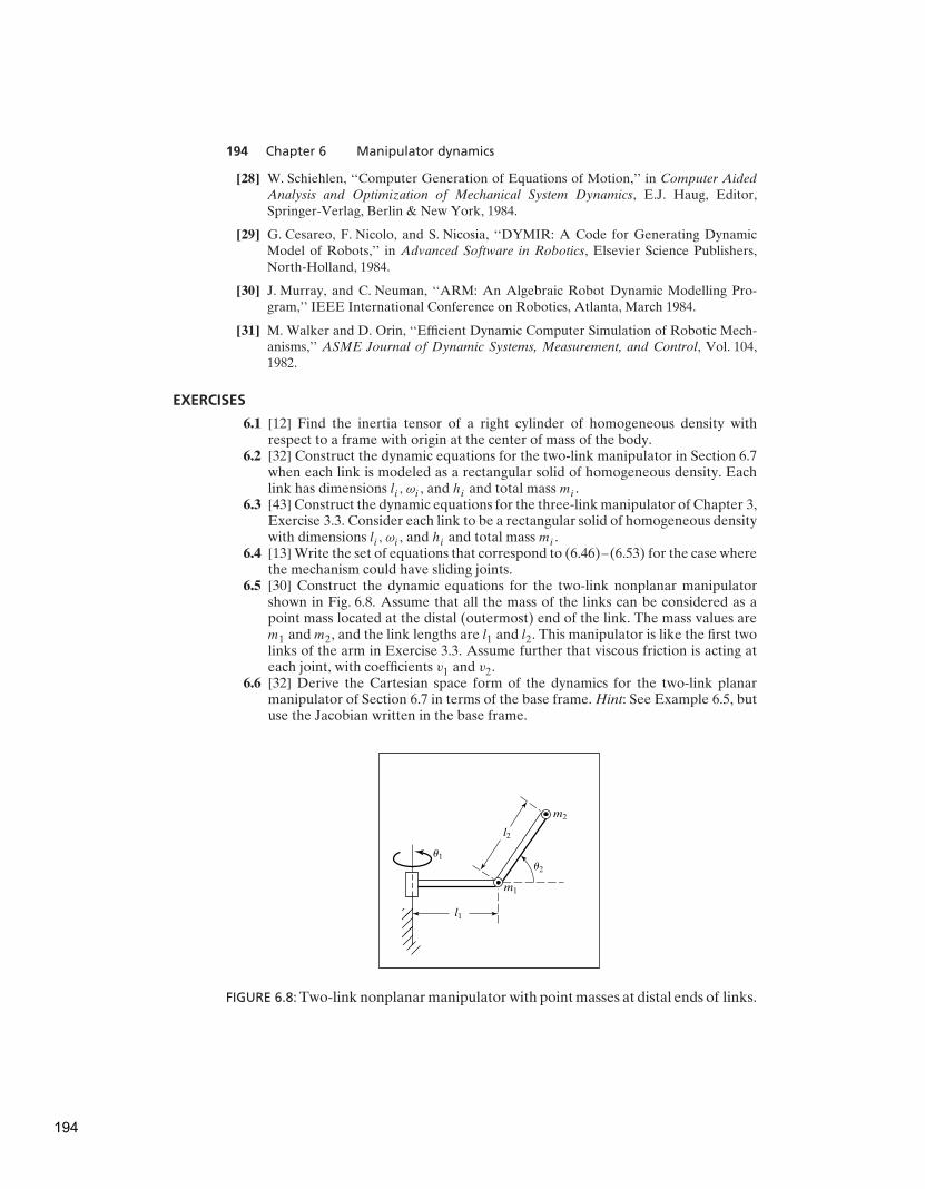
194 Chapter 6 Manipulator dynamics
[28] W. Schiehlen, ‘‘Computer Generation of Equations of Motion,’’ in Computer Aided
Analysis and Optimization of Mechanical System Dynamics, E.J. Haug, Editor,Springer-Verlag, Berlin & New York, 1984.
[29] G. Cesareo, F. Nicolo, and S. Nicosia, ‘‘DYMIR: A Code for Generating DynamicModel of Robots,’’ in Advanced Software in Robotics, Elsevier Science Publishers,North-Holland, 1984.
[30] J. Murray, and C. Neuman, ‘‘ARM: An Algebraic Robot Dynamic Modelling Pro-gram,’’ IEEE International Conference on Robotics, Atlanta, March 1984.
[31] M. Walker and D. Orin, ‘‘Efficient Dynamic Computer Simulation of Robotic Mech-anisms,’’ ASME Journal of Dynamic Systems, Measurement, and Control, Vol. 104,1982.
EXERCISES
6.1 [12] Find the inertia tensor of a right cylinder of homogeneous density withrespect to a frame with origin at the center of mass of the body.
6.2 [32] Construct the dynamic equations for the two-link manipulator in Section 6.7when each link is modeled as a rectangular solid of homogeneous density. Eachlink has dimensions li, ωi , and hi and total mass mi .
6.3 [43] Construct the dynamic equations for the three-link manipulator of Chapter 3,Exercise 3.3. Consider each link to be a rectangular solid of homogeneous densitywith dimensions li, ωi , and hi and total mass mi .
6.4 [13] Write the set of equations that correspond to (6.46)–(6.53) for the case wherethe mechanism could have sliding joints.
6.5 [30] Construct the dynamic equations for the two-link nonplanar manipulatorshown in Fig. 6.8. Assume that all the mass of the links can be considered as apoint mass located at the distal (outermost) end of the link. The mass values arem1 andm2, and the link lengths are l1 and l2. This manipulator is like the first twolinks of the arm in Exercise 3.3. Assume further that viscous friction is acting ateach joint, with coefficients v1 and v2.
6.6 [32] Derive the Cartesian space form of the dynamics for the two-link planarmanipulator of Section 6.7 in terms of the base frame. Hint: See Example 6.5, butuse the Jacobian written in the base frame.
l2
u2
u1
l1
m2
m1
FIGURE 6.8: Two-link nonplanar manipulator with point masses at distal ends of links.
194

Exercises 195
6.7 [18] How many memory locations would be required to store the dynamicequations of a general three-link manipulator in a table? Quantize each joint’sposition, velocity, and acceleration into 16 ranges. Make any assumptions needed.
6.8 [32] Derive the dynamic equations for the two-link manipulator shown in Fig. 4.6.Link 1 has an inertia tensor given by
C1I =
Ixx1 0 00 Iyy1 00 0 Izz1
.
Assume that link 2 has all its mass, m2, located at a point at the end-effector.
Assume that gravity is directed downward (opposite Z1).6.9 [37] Derive the dynamic equations for the three-link manipulator with one
prismatic joint shown in Fig. 3.9. Link 1 has an inertia tensor given by
C1I =
Ixx1 0 00 Iyy1 00 0 Izz1
.
Link 2 has point mass m2 located at the origin of its link frame. Link 3 has aninertia tensor given by
C3I =
Ixx3 0 00 Iyy3 00 0 Izz3
.
Assume that gravity is directed opposite Z1 and that viscous friction of magnitudevi is active at each joint.
6.10 [35] Derive the dynamic equations in Cartesian space for the manipulator ofExercise 6.8. Write the equations in frame {2}.
6.11 [20] A certain one-link manipulator has
C1I =
Ixx1 0 00 Iyy1 00 0 Izz1
.
Assume that this is just the inertia of the link itself. If the motor armature has amoment of inertia Im and the gear ratio is 100, what is the total inertia as seenfrom the motor shaft [1]?
6.12 [20] The single-degree-of-freedom ‘‘manipulator’’ in Fig. 6.9 has total massm = 1,with the center of mass at
1PC =
200
,
and has inertia tensor
CI1 =
1 0 00 2 00 0 2
.
From rest at t = 0, the joint angle θ1 moves in accordance with the time function
θ1(t) = bt + ct2
in radians. Give the angular acceleration of the link and the linear acceleration ofthe center of mass in terms of frame {1} as a function of t .
195

196 Chapter 6 Manipulator dynamics
X0
Y0
Pcl
u1
Z0
FIGURE 6.9: One-link ‘‘manipulator’’ of Exercise 6.12.
6.13 [40] Construct the Cartesian dynamic equations for the two-link nonplanarmanipulator shown in Fig. 6.8. Assume that all the mass of the links can beconsidered as a point mass located at the distal (outermost) end of the link. Themass values are m1 and m2, and the link lengths are l1 and l2. This manipulator islike the first two links of the arm in Exercise 3.3. Also assume that viscous frictionis acting at each joint with coefficients v1 and v2. Write the Cartesian dynamicsin frame {3}, which is located at the tip of the manipulator and has the sameorientation as link frame {2}.
6.14 [18] The following equations were derived for a 2-DOF RP manipulator:
τ1 = m1(d21
+ d2)θ1 +m2d22θ1 + 2m2d2d2θ1
+g cos(θ1)[m1(d1 + d2θ1)+m2(d2 + d2)]
τ2 = m1d2θ1 +m2d2 −m1d1d2 −m2d2θ2 +m2(d2 + 1)g sin(θ1).
Some of the terms are obviously incorrect. Indicate the incorrect terms.6.15 [28] Derive the dynamic equations for the RP manipulator of Example 6.5, using
the Newton–Euler procedure instead of the Lagrangian technique.6.16 [25] Derive the equations of motion for the PR manipulator shown in Fig. 6.10.
Neglect friction, but include gravity. (Here, X0 is upward.) The inertia tensorsof the links are diagonal, with moments Ixx1, Iyy1, Izz1 and Ixx2, Iyy2, Izz2. Thecenters of mass for the links are given by
1PC1=
00
−l1
,
2PC2=
000
.
6.17 [40] The velocity-related terms appearing in the manipulator dynamic equationcan be written as a matrix-vector product—that is,
V (�, �) = Vm(�, �)�,
196

Programming exercise (Part 6) 197
X0Y2
m1 m2
Z0
X1
X2
Z1
FIGURE 6.10: PR manipulator of Exercise 6.16.
where the m subscript stands for ‘‘matrix form.’’ Show that an interesting rela-tionship exists between the time derivative of the manipulator mass matrix andVm(·), namely,
M(�) = 2Vm(�, �)− S,
where S is some skew-symmetric matrix.6.18 [15] Give two properties that any reasonable friction model (i.e., the termF(�, �)
in (6.114)) would possess.6.19 [28] Do Exercise 6.5, using Lagrange’s equations.6.20 [28] Derive the dynamic equations of the 2-DOF manipulator of Section 6.7, using
a Lagrangian formulation.
PROGRAMMING EXERCISE (PART 6)
1. Derive the dynamic equations of motion for the three-link manipulator (fromExample 3.3). That is, expand Section 6.7 for the three-link case. The followingnumerical values describe the manipulator:
l1 = l2 = 0.5m,
m1 = 4.6Kg,
m2 = 2.3Kg,
m3 = 1.0Kg,
g = 9.8m/s2.
For the first two links, we assume that the mass is all concentrated at the distal endof the link. For link 3, we assume that the center of mass is located at the origin offrame {3}—that is, at the proximal end of the link. The inertia tensor for link 3 is
Cs I =
0.05 0 00 0.1 00 0 0.1
Kg-m2.
197

198 Chapter 6 Manipulator dynamics
The vectors that locate each center of mass relative to the respective link frameare
1PC1= l1X1,
2PC2= l2X2,
3PC3= 0.
2. Write a simulator for the three-link manipulator. A simple Euler-integrationroutine is sufficient for performing the numerical integration (as in Section 6.12).To keep your code modular, it might be helpful to define the routine
Procedure UPDATE(VAR tau: vec3; VAR period: real; VAR
theta, thetadot: vec3);
where ‘‘tau’’ is the torque command to the manipulator (always zero for thisassignment), ‘‘period’’ is the length of time you wish to advance time (in seconds),and ‘‘theta’’ and ‘‘thetadot’’ are the state of the manipulator. Theta and thetadotare updated by ‘‘period’’ seconds each time you call UPDATE. Note that ‘‘period’’would typically be longer than the integration step size, t , used in the numericalintegration. For example, although the step size for numerical integration mightbe 0.001 second, you might wish to print out the manipulator position and velocityonly each 0.1 seconds.
To test your simulation, set the joint-torque commands to zero (for all time) andperform these tests:
(a) Set the initial position of the manipulator to
[θ1 θ2 θ3] = [−90 0 0].
Simulate for a few seconds. Is the motion of the manipulator what you wouldexpect?
(b) Set the initial position of the manipulator to
[θ1 θ2 θ3] = [30 30 10].
Simulate for a few seconds. Is the motion of the manipulator what you wouldexpect?
(c) Introduce some viscous friction at each joint of the simulated manipula-tor—that is, add a term to the dynamics of each joint in the form τf = vθ ,where v = 5.0 newton-meter-seconds for each joint. Repeat test (b) above.Is the motion what you would expect?
MATLAB EXERCISE 6A
This exercise focuses on the inverse-dynamics analysis (in a resolved-rate controlframework—see MATLAB Exercise 5) for the planar 2-DOF 2R robot. This robot isthe first two R-joints and first two moving links of the planar 3-DOF 3R robot. (SeeFigures 3.6 and 3.7; the DH parameters are given in the first two rows of Figure 3.8.)
For the planar 2R robot, calculate the required joint torques (i.e., solve theinverse-dynamics problem) to provide the commanded motion at every time step in aresolved-rate control scheme. You can use either numerical Newton–Euler recursion orthe analytical equations from the results of Exercise 6.2, or both.
198

MATLAB Exercise 6C 199
Given: L1 = 1.0 m, L2 = 0.5 m; Both links are solid steel with mass densityρ = 7806 kg/m3; both have the width and thickness dimensions w = t = 5 cm. Therevolute joints are assumed to be perfect, connecting the links at their very edges (notphysically possible).
The initial angles are � =
{
θ1θ2
}
=
{
10◦
90◦
}
.
The (constant) commanded Cartesian velocity is 0X = 0
{
x
y
}
= 0
{
00.5
}
(m/s).
Simulate motion for 1 sec, with a control time step of 0.01 sec.Present five plots (each set on a separate graph, please):
1. the two joint angles (degrees) � = {θ1 θ2}T vs. time;
2. the two joint rates (rad/s) � = {θ1 θ2}T vs. time;
3. the two joint accelerations (rad/s2) � = {θ1 θ2}T vs. time;
4. the three Cartesian components of 0HT , X = {x y φ}T (rad is fine for φ so it will
fit) vs. time;
5. the two inverse dynamics joint torques (Nm) T = {τ1 τ2}T vs. time.
Carefully label (by hand is fine!) each component on each plot. Also, label the axisnames and units.
Perform this simulation twice. The first time, ignore gravity (the motion plane isnormal to the effect of gravity); the second time, consider gravity g in the negative Ydirection.
MATLAB EXERCISE 6B
This exercise focuses on the inverse-dynamics solution for the planar 3-DOF, 3R robot (ofFigures 3.6 and 3.7; the DH parameters are given in Figure 3.8) for a motion snapshot intime only. The following fixed-length parameters are given: L1 = 4, L2 = 3, and L3 = 2(m). For dynamics, we must also be given mass and moment-of-inertia information:m1 = 20, m2 = 15, m3 = 10 (kg), CIZZ1 = 0.5, CIZZ2 = 0.2, and CIZZ3 = 0.1 (kgm2).Assume that the CG of each link is in its geometric center. Also, assume that gravity actsin the −Y direction in the plane of motion. For this exercise, ignore actuator dynamicsand the joint gearing.
a) Write a MATLAB program to implement the recursive Newton–Euler inverse-dynamics solution (i.e., given the commanded motion, calculate the requireddriving joint torques) for the following motion snapshot in time:
� =
θ1θ2θ3
=
10◦
20◦
30◦
� =
θ1θ2θ3
=
123
(rad/s)� =
θ1θ2θ3
=
0.51
1.5
(rad/s2)
b) Check your results in (a) by means of the Corke MATLAB Robotics Toolbox. Tryfunctions rne() and gravload().
MATLAB EXERCISE 6C
This exercise focuses on the forward-dynamics solution for the planar 3-DOF, 3R robot(parameters from MATLAB Exercise 6B) for motion over time. In this case, ignoregravity (i.e., assume that gravity acts in a direction normal to the plane of motion). Usethe Corke MATLAB Robotics Toolbox to solve the forward-dynamics problem (i.e.,
199
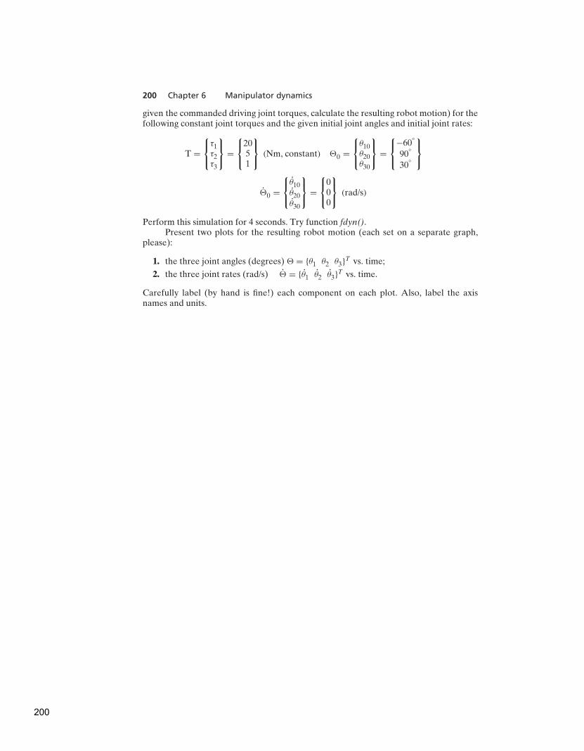
200 Chapter 6 Manipulator dynamics
given the commanded driving joint torques, calculate the resulting robot motion) for thefollowing constant joint torques and the given initial joint angles and initial joint rates:
T =
τ1τ2τ3
=
2051
(Nm, constant) �0 =
θ10θ20θ30
=
−60◦
90◦
30◦
�0 =
θ10θ20θ30
=
000
(rad/s)
Perform this simulation for 4 seconds. Try function fdyn().Present two plots for the resulting robot motion (each set on a separate graph,
please):
1. the three joint angles (degrees) � = {θ1 θ2 θ3}T vs. time;
2. the three joint rates (rad/s) � = {θ1 θ2 θ3}T vs. time.
Carefully label (by hand is fine!) each component on each plot. Also, label the axisnames and units.
200

C H A P T E R 7
Trajectory generation
7.1 INTRODUCTION
7.2 GENERAL CONSIDERATIONS IN PATH DESCRIPTION AND GENERATION
7.3 JOINT-SPACE SCHEMES
7.4 CARTESIAN-SPACE SCHEMES
7.5 GEOMETRIC PROBLEMS WITH CARTESIAN PATHS
7.6 PATH GENERATION AT RUN TIME
7.7 DESCRIPTION OF PATHS WITH A ROBOT PROGRAMMING LANGUAGE
7.8 PLANNING PATHS WHEN USING THE DYNAMIC MODEL
7.9 COLLISION-FREE PATH PLANNING
7.1 INTRODUCTION
In this chapter, we concern ourselves with methods of computing a trajectory thatdescribes the desired motion of a manipulator in multidimensional space. Here,trajectory refers to a time history of position, velocity, and acceleration for eachdegree of freedom.
This problem includes the human-interface problem of how we wish to specify
a trajectory or path through space. In order to make the description of manipulatormotion easy for a human user of a robot system, the user should not be requiredto write down complicated functions of space and time to specify the task. Rather,we must allow the capability of specifying trajectories with simple descriptions ofthe desired motion, and let the system figure out the details. For example, the usermight want to be able to specify nothing more than the desired goal position andorientation of the end-effector and leave it to the system to decide on the exactshape of the path to get there, the duration, the velocity profile, and other details.
We also are concerned with how trajectories are represented in the computerafter they have been planned. Finally, there is the problem of actually comput-ing the trajectory from the internal representation—or generating the trajectory.Generation occurs at run time; in the most general case, position, velocity, andacceleration are computed. These trajectories are computed on digital computers,so the trajectory points are computed at a certain rate, called the path-update rate.In typical manipulator systems, this rate lies between 60 and 2000 Hz.
7.2 GENERAL CONSIDERATIONS IN PATH DESCRIPTION AND GENERATION
For the most part, we will consider motions of a manipulator as motions ofthe tool frame, {T }, relative to the station frame, {S}. This is the same manner
From Chapter 7 of Introduction to Robotics: Mechanics and Control, Third Edition. John J. Craig.
Copyright © 2005 by Pearson Education, Inc. All rights reserved.
201

202 Chapter 7 Trajectory generation
in which an eventual user of the system would think, and designing a pathdescription and generation system in these terms will result in a few importantadvantages.
When we specify paths as motions of the tool frame relative to the stationframe, we decouple the motion description from any particular robot, end-effector,or workpieces. This results in a certain modularity and would allow the same pathdescription to be used with a different manipulator—or with the same manipulator,but a different tool size. Further, we can specify and plan motions relative to amoving workstation (perhaps a conveyor belt) by planning motions relative to thestation frame as always and, at run time, causing the definition of {S} to be changingwith time.
As shown in Fig. 7.1, the basic problem is to move the manipulator from aninitial position to some desired final position—that is, we wish to move the toolframe from its current value, {Tinitial}, to a desired final value, {Tfinal}. Note that,in general, this motion involves both a change in orientation and a change in theposition of the tool relative to the station.
Sometimes it is necessary to specify the motion in much more detail thanby simply stating the desired final configuration. One way to include more detailin a path description is to give a sequence of desired via points (intermediatepoints between the initial and final positions). Thus, in completing the motion, thetool frame must pass through a set of intermediate positions and orientations asdescribed by the via points. Each of these via points is actually a frame that specifiesboth the position and orientation of the tool relative to the station. The namepath points includes all the via points plus the initial and final points. Rememberthat, although we generally use the term ‘‘points,’’ these are actually frames, whichgive both position and orientation. Along with these spatial constraints on themotion, the user could also wish to specify temporal attributes of the motion. Forexample, the time elapsed between via points might be specified in the descriptionof the path.
Usually, it is desirable for the motion of the manipulator to be smooth. Forour purposes, we will define a smooth function as a function that is continuous andhas a continuous first derivative. Sometimes a continuous second derivative is also
FIGURE 7.1: In executing a trajectory, a manipulator moves from its initial positionto a desired goal position in a smooth manner.
202
Section 7.3 Joint-space schemes 203
desirable. Rough, jerky motions tend to cause increased wear on the mechanism andcause vibrations by exciting resonances in the manipulator. In order to guaranteesmooth paths, we must put some sort of constraints on the spatial and temporalqualities of the path between the via points.
At this point, there are many choices that may be made and, consequently,a great variety in the ways that paths might be specified and planned. Anysmooth functions of time that pass through the via points could be used tospecify the exact path shape. In this chapter, we will discuss a couple of sim-ple choices for these functions. Other approaches can be found in [1, 2] and[13–16].
7.3 JOINT-SPACE SCHEMES
In this section, we consider methods of path generation in which the path shapes (inspace and in time) are described in terms of functions of joint angles.
Each path point is usually specified in terms of a desired position and ori-entation of the tool frame, {T }, relative to the station frame, {S}. Each of thesevia points is ‘‘converted’’ into a set of desired joint angles by application of theinverse kinematics. Then a smooth function is found for each of the n joints thatpass through the via points and end at the goal point. The time required for eachsegment is the same for each joint so that all joints will reach the via point at thesame time, thus resulting in the desired Cartesian position of {T } at each via point.Other than specifying the same duration for each joint, the determination of thedesired joint angle function for a particular joint does not depend on the functionsfor the other joints.
Hence, joint-space schemes achieve the desired position and orientation at thevia points. In between via points, the shape of the path, although rather simple in jointspace, is complex if described in Cartesian space. Joint-space schemes are usually theeasiest to compute, and, because we make no continuous correspondence betweenjoint space and Cartesian space, there is essentially no problem with singularities ofthe mechanism.
Cubic polynomials
Consider the problem of moving the tool from its initial position to a goal positionin a certain amount of time. Inverse kinematics allow the set of joint angles thatcorrespond to the goal position and orientation to be calculated. The initial positionof the manipulator is also known in the form of a set of joint angles. What is requiredis a function for each joint whose value at t0 is the initial position of the joint andwhose value at tf is the desired goal position of that joint. As shown in Fig. 7.2,there are many smooth functions, θ(t), that might be used to interpolate the jointvalue.
In making a single smooth motion, at least four constraints on θ(t) are evident.Two constraints on the function’s value come from the selection of initial andfinal values:
θ(0) = θ0,
θ(tf ) = θf . (7.1)
203

204 Chapter 7 Trajectory generation
u(t)
uf
u0
ttft0
FIGURE 7.2: Several possible path shapes for a single joint.
An additional two constraints are that the function be continuous in velocity, whichin this case means that the initial and final velocity are zero:
θ (0) = 0,
θ (tf ) = 0. (7.2)
These four constraints can be satisfied by a polynomial of at least third degree.(A cubic polynomial has four coefficients, so it can be made to satisfy the fourconstraints given by (7.1) and (7.2).) These constraints uniquely specify a particularcubic. A cubic has the form
θ(t) = a0 + a1t + a2t2 + a3t
3, (7.3)
so the joint velocity and acceleration along this path are clearly
θ (t) = a1 + 2a2t + 3a3t2,
θ (t) = 2a2 + 6a3t. (7.4)
Combining (7.3) and (7.4) with the four desired constraints yields four equations infour unknowns:
θ0 = a0,
θf = a0 + a1tf + a2t2f
+ a3t3f,
0 = a1, (7.5)
0 = a1 + 2a2tf + 3a3t2f.
Solving these equations for the ai , we obtain
a0 = θ0,
a1 = 0,
204
Section 7.3 Joint-space schemes 205
a2 =3
t2f
(θf − θ0), (7.6)
a3 = −2
t3f
(θf − θ0).
Using (7.6), we can calculate the cubic polynomial that connects any initial joint-angle position with any desired final position. This solution is for the case when thejoint starts and finishes at zero velocity.
EXAMPLE 7.1
A single-link robot with a rotary joint is motionless at θ = 15 degrees. It is desiredto move the joint in a smooth manner to θ = 75 degrees in 3 seconds. Find thecoefficients of a cubic that accomplishes this motion and brings the manipulator torest at the goal. Plot the position, velocity, and acceleration of the joint as a functionof time.
Plugging into (7.6), we find that
a0 = 15.0,
a1 = 0.0,
a2 = 20.0, (7.7)
a3 = −4.44.
Using (7.3) and (7.4), we obtain
θ(t) = 15.0 + 20.0t2 − 4.44t3,
θ(t) = 40.0t − 13.33t2, (7.8)
θ (t) = 40.0 − 26.66t.
Figure 7.3 shows the position, velocity, and acceleration functions for this motionsampled at 40 Hz. Note that the velocity profile for any cubic function is a parabolaand that the acceleration profile is linear.
Cubic polynomials for a path with via points
So far, we have considered motions described by a desired duration and a final goalpoint. In general, we wish to allow paths to be specified that include intermediatevia points. If the manipulator is to come to rest at each via point, then we can usethe cubic solution of Section 7.3.
Usually, we wish to be able to pass through a via point without stopping, andso we need to generalize the way in which we fit cubics to the path constraints.
As in the case of a single goal point, each via point is usually specified interms of a desired position and orientation of the tool frame relative to the stationframe. Each of these via points is ‘‘converted’’ into a set of desired joint angles byapplication of the inverse kinematics. We then consider the problem of computingcubics that connect the via-point values for each joint together in a smooth way.
205

206 Chapter 7 Trajectory generation
15202530354045505560657075
.6 1.2 1.8
Position
Seconds
Degrees
2.4 3.0
0
5
10
15
20
25
30
.6 1.2 1.8
Velocity
Seconds
Deg/sec
2.4 3.0
�40
�25
�15
�5
10
25
403530
20
5
�10
�20
�30�35
0
15
.6 1.2 1.8
Acceleration
Seconds
Deg/sec2
2.4 3.0
FIGURE 7.3: Position, velocity, and acceleration profiles for a single cubic segmentthat starts and ends at rest.
If desired velocities of the joints at the via points are known, then we canconstruct cubic polynomials as before; now, however, the velocity constraints at eachend are not zero, but rather, some known velocity. The constraints of (7.3) become
θ (0) = θ0,
θ (tf ) = θf . (7.9)
206
Section 7.3 Joint-space schemes 207
The four equations describing this general cubic are
θ0 = a0,
θf = a0 + a1tf + a2t2f
+ a3t3f,
θ0 = a1, (7.10)
θf = a1 + 2a2tf + 3a3t2f.
Solving these equations for the ai , we obtain
a0 = θ0,
a1 = θ0,
a2 =3
t2f
(θf − θ0)−2
tfθ0 −
1
tfθf , (7.11)
a3 = −2
t3f
(θf − θ0)+1
t2f
(θf + θ0).
Using (7.11), we can calculate the cubic polynomial that connects any initial andfinal positions with any initial and final velocities.
If we have the desired joint velocities at each via point, then we simply apply(7.11) to each segment to find the required cubics. There are several ways in whichthe desired velocity at the via points might be specified:
1. The user specifies the desired velocity at each via point in terms of a Cartesianlinear and angular velocity of the tool frame at that instant.
2. The system automatically chooses the velocities at the via points by applyinga suitable heuristic in either Cartesian space or joint space.
3. The system automatically chooses the velocities at the via points in such a wayas to cause the acceleration at the via points to be continuous.
In the first option, Cartesian desired velocities at the via points are ‘‘mapped’’to desired joint rates by using the inverse Jacobian of the manipulator evaluatedat the via point. If the manipulator is at a singular point at a particular via point,then the user is not free to assign an arbitrary velocity at this point. It is a usefulcapability of a path-generation scheme to be able to meet a desired velocity that theuser specifies, but it would be a burden to require that the user always make thesespecifications. Therefore, a convenient system should include either option 2 or 3(or both).
In option 2, the system automatically chooses reasonable intermediate veloc-ities, using some kind of heuristic. Consider the path specified by the via pointsshown for some joint, θ , in Fig. 7.4.
In Fig. 7.4, we have made a reasonable choice of joint velocities at the via points,as indicated with small line segments representing tangents to the curve at eachvia point. This choice is the result of applying a conceptually and computationallysimple heuristic. Imagine the via points connected with straight line segments. If the
207
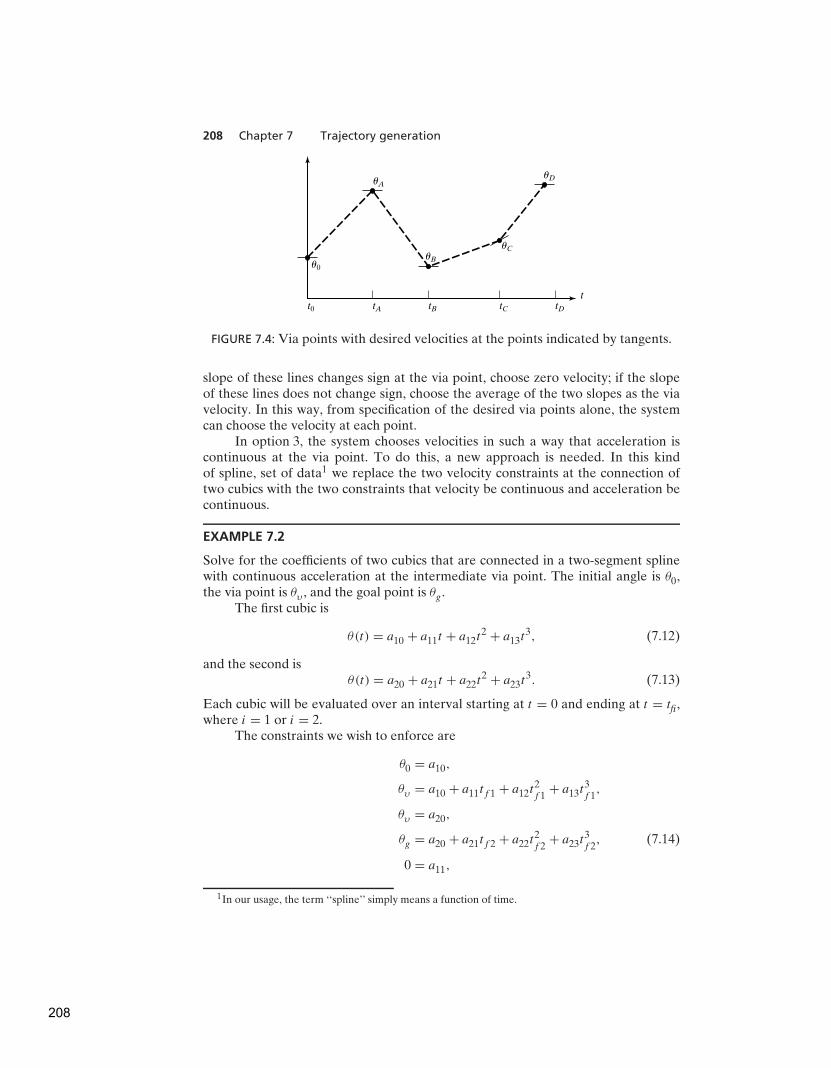
208 Chapter 7 Trajectory generation
uB
uC
uD
u0
uA
tt0 tA tB tC tD
FIGURE 7.4: Via points with desired velocities at the points indicated by tangents.
slope of these lines changes sign at the via point, choose zero velocity; if the slopeof these lines does not change sign, choose the average of the two slopes as the viavelocity. In this way, from specification of the desired via points alone, the systemcan choose the velocity at each point.
In option 3, the system chooses velocities in such a way that acceleration iscontinuous at the via point. To do this, a new approach is needed. In this kindof spline, set of data1 we replace the two velocity constraints at the connection oftwo cubics with the two constraints that velocity be continuous and acceleration becontinuous.
EXAMPLE 7.2
Solve for the coefficients of two cubics that are connected in a two-segment splinewith continuous acceleration at the intermediate via point. The initial angle is θ0,the via point is θυ , and the goal point is θg .
The first cubic is
θ(t) = a10 + a11t + a12t2 + a13t
3, (7.12)
and the second isθ(t) = a20 + a21t + a22t
2 + a23t3. (7.13)
Each cubic will be evaluated over an interval starting at t = 0 and ending at t = tfi,where i = 1 or i = 2.
The constraints we wish to enforce are
θ0 = a10,
θυ = a10 + a11tf 1 + a12t2f 1
+ a13t3f 1,
θυ = a20,
θg = a20 + a21tf 2 + a22t2f 2
+ a23t3f 2, (7.14)
0 = a11,
1In our usage, the term ‘‘spline’’ simply means a function of time.
208

Section 7.3 Joint-space schemes 209
0 = a21 + 2a22tf 2 + 3a23t2f 2,
a11 + 2a12tf 1 + 3a12t2f 1
= a21,
2a12 + 6a13tf 1 = 2a22.
These constraints specify a linear-equation problem having eight equations andeight unknowns. Solving for the case tf = tf 1 = tf 2, we obtain
a10 = θ0,
a11 = 0,
a12 =12θυ − 3θg − 9θ0
4t2f
,
a13 =−8θυ + 3θg + 5θ0
4t3f
,
a20 = θυ , (7.15)
a21 =3θg − 3θ0
4tf,
a22 =−12θυ + 6θg + 6θ0
4t2f
,
a23 =8θυ − 5θg − 3θ0
4t3f
.
For the general case, involving n cubic segments, the equations that arise frominsisting on continuous acceleration at the via points can be cast in matrix form,which is solved to compute the velocities at the via points. The matrix turns out tobe tridiagonal and easily solved [4].
Higher-order polynomials
Higher-order polynomials are sometimes used for path segments. For exam-ple, if we wish to be able to specify the position, velocity, and accelerationat the beginning and end of a path segment, a quintic polynomial is required,namely,
θ(t) = a0 + a1t + a2t2 + a3t
3 + a4t4 + a5t
5, (7.16)
where the constraints are given as
θ0 = a0,
θf = a0 + a1tf + a2t2f
+ a3t3f
+ a4t4f
+ a5t5f,
209
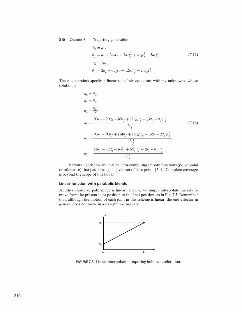
210 Chapter 7 Trajectory generation
θ0 = a1,
θf = a1 + 2a2tf + 3a3t2f
+ 4a4t3f
+ 5a5t4f, (7.17)
θ0 = 2a2,
θf = 2a2 + 6a3tf + 12a4t2f
+ 20a5t3f.
These constraints specify a linear set of six equations with six unknowns, whosesolution is
a0 = θ0,
a1 = θ0,
a2 =θ0
2,
a3 =20θf − 20θ0 − (8θf + 12θ0)tf − (3θ0 − θf )t
2f
2t3f
, (7.18)
a4 =30θ0 − 30θf + (14θf + 16θ0)tf + (3θ0 − 2θf )t
2f
2t4f
,
a5 =12θf − 12θ0 − (6θf + 6θ0)tf − (θ0 − θf )t
2f
2t5f
.
Various algorithms are available for computing smooth functions (polynomialor otherwise) that pass through a given set of data points [3, 4]. Complete coverageis beyond the scope of this book.
Linear function with parabolic blends
Another choice of path shape is linear. That is, we simply interpolate linearly tomove from the present joint position to the final position, as in Fig. 7.5. Rememberthat, although the motion of each joint in this scheme is linear, the end-effector ingeneral does not move in a straight line in space.
u
uf
u0
ttft0
FIGURE 7.5: Linear interpolation requiring infinite acceleration.
210

Section 7.3 Joint-space schemes 211
However, straightforward linear interpolation would cause the velocity to bediscontinuous at the beginning and end of the motion. To create a smooth pathwith continuous position and velocity, we start with the linear function but add aparabolic blend region at each path point.
During the blend portion of the trajectory, constant acceleration is used tochange velocity smoothly. Figure 7.6 shows a simple path constructed in this way.The linear function and the two parabolic functions are ‘‘splined’’ together so thatthe entire path is continuous in position and velocity.
In order to construct this single segment, we will assume that the parabolicblends both have the same duration; therefore, the same constant acceleration(modulo a sign) is used during both blends. As indicated in Fig. 7.7, there are manysolutions to the problem—but note that the answer is always symmetric about thehalfway point in time, th, and about the halfway point in position, θh. The velocityat the end of the blend region must equal the velocity of the linear section, and sowe have
θ tb =θh − θb
th − tb, (7.19)
where θb is the value of θ at the end of the blend region, and θ is the accelerationacting during the blend region. The value of θb is given by
θb = θ0 + 12 θ t
2b. (7.20)
u
uf
u0
ttft0 tb tf � tb
FIGURE 7.6: Linear segment with parabolic blends.
u
uf
uh
u0
ttft0 th
FIGURE 7.7: Linear segment with parabolic blends.
211
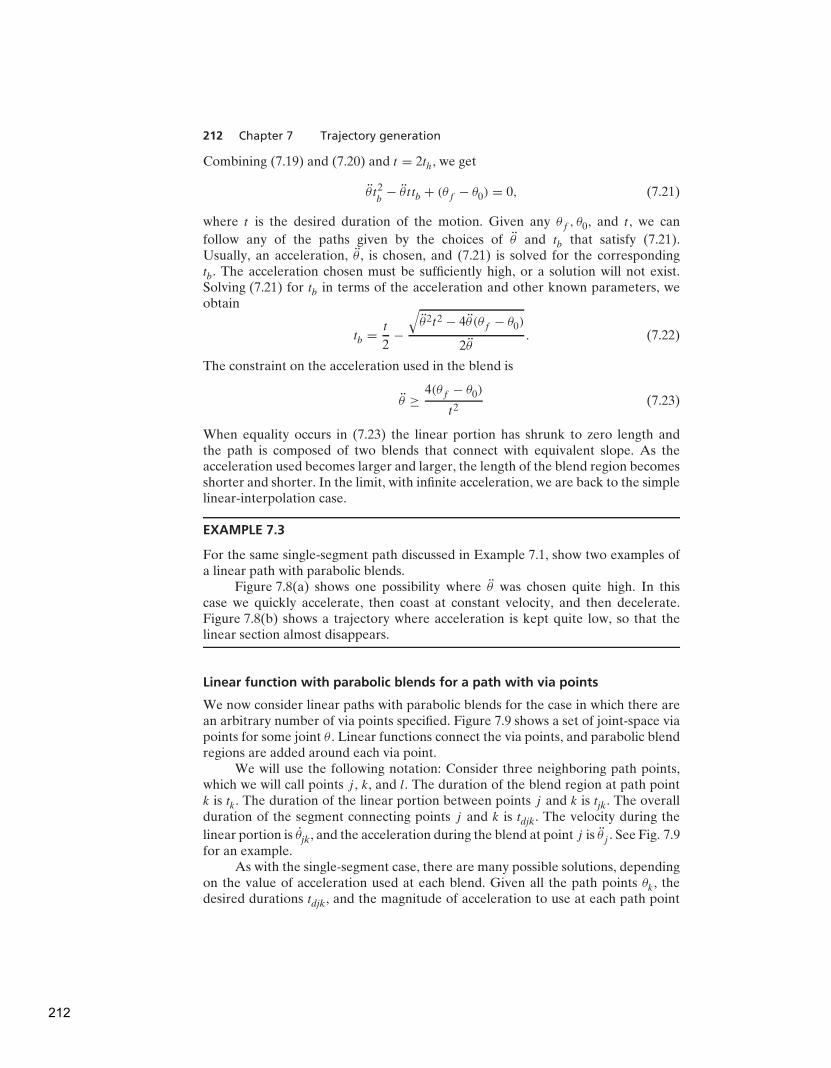
212 Chapter 7 Trajectory generation
Combining (7.19) and (7.20) and t = 2th, we get
θ t2b
− θ t tb + (θf − θ0) = 0, (7.21)
where t is the desired duration of the motion. Given any θf , θ0, and t , we can
follow any of the paths given by the choices of θ and tb that satisfy (7.21).Usually, an acceleration, θ , is chosen, and (7.21) is solved for the correspondingtb. The acceleration chosen must be sufficiently high, or a solution will not exist.Solving (7.21) for tb in terms of the acceleration and other known parameters, weobtain
tb =t
2−
√
θ2t2 − 4θ (θf − θ0)
2θ. (7.22)
The constraint on the acceleration used in the blend is
θ ≥4(θf − θ0)
t2(7.23)
When equality occurs in (7.23) the linear portion has shrunk to zero length andthe path is composed of two blends that connect with equivalent slope. As theacceleration used becomes larger and larger, the length of the blend region becomesshorter and shorter. In the limit, with infinite acceleration, we are back to the simplelinear-interpolation case.
EXAMPLE 7.3
For the same single-segment path discussed in Example 7.1, show two examples ofa linear path with parabolic blends.
Figure 7.8(a) shows one possibility where θ was chosen quite high. In thiscase we quickly accelerate, then coast at constant velocity, and then decelerate.Figure 7.8(b) shows a trajectory where acceleration is kept quite low, so that thelinear section almost disappears.
Linear function with parabolic blends for a path with via points
We now consider linear paths with parabolic blends for the case in which there arean arbitrary number of via points specified. Figure 7.9 shows a set of joint-space viapoints for some joint θ . Linear functions connect the via points, and parabolic blendregions are added around each via point.
We will use the following notation: Consider three neighboring path points,which we will call points j , k, and l. The duration of the blend region at path pointk is tk . The duration of the linear portion between points j and k is tjk. The overallduration of the segment connecting points j and k is tdjk. The velocity during the
linear portion is θjk, and the acceleration during the blend at point j is θj . See Fig. 7.9for an example.
As with the single-segment case, there are many possible solutions, dependingon the value of acceleration used at each blend. Given all the path points θk , thedesired durations tdjk, and the magnitude of acceleration to use at each path point
212

Section 7.3 Joint-space schemes 213
152025303540455055606570
.6 1.2 1.8
Position
Seconds
Degrees
2.4 3.0152025303540455055606570
.6 1.2 1.8
Position
Seconds
Degrees
2.4 3.0
0
5
10
15
20
.6 1.2 1.8
Velocity
Seconds
Deg/sec
2.4 3.00
15
10
20
25
5
30
35
.6 1.2 1.8
Velocity
Seconds
Deg/sec
2.4 3.0
�36
�24
�12
0
36
24
12
.6 1.2 1.8
Acceleration
(a)
Acceleration
(b)
Seconds
Deg/sec2
2.4 3.0
�25
�5
�15
5
1510
0
�10
�20
2025
.6 1.2 1.8Seconds
Deg/sec2
2.4 3.0
FIGURE 7.8: Position, velocity, and acceleration profiles for linear interpolation withparabolic blends. The set of curves on the left is based on a higher accelerationduring the blends than is that on the right.
|θk|, we can compute the blend times tk . For interior path points, this follows simplyfrom the equations
θjk =θk − θj
tdjk,
θk = SGN(θkl − θjk)|θk|,
tk =θkl − θjk
θk, (7.24)
tjk = tdjk −1
2tj −
1
2tk.
213

214 Chapter 7 Trajectory generation
u
ui
ul
uj
uk
t
tk
tjk
td12 tdjk
Slope � ujk
Slope � ukl
FIGURE 7.9: Multisegment linear path with blends.
The first and last segments must be handled slightly differently, because an entireblend region at one end of the segment must be counted in the total segment’s timeduration.
For the first segment, we solve for t1 by equating two expressions for thevelocity during the linear phase of the segment:
θ2 − θ1
t12 − 12 t1
= θ1t1. (7.25)
This can be solved for t1, the blend time at the initial point; then θ12 and t12 are easilycomputed:
θ1 = SGN(θ2 − θ1)|θ1|,
t1 = td12 −
√
t2d12
−2(θ2 − θ1)
θ1
,
θ12 =θ2 − θ1
td12 − 12 t1
, (7.26)
t12 = td12 − t1 −1
2t2.
Likewise, for the last segment (the one connecting points n−1 and n), we have
θn−1 − θn
td(n−1)n − 12 tn
= θntn, (7.27)
which leads to the solution
θn = SGN(θn−1 − θn)|θn|,
tn = td(n−1)n −
√
t2d(n−1)n
+2(θn − θn−1)
θn,
214

Section 7.3 Joint-space schemes 215
θ(n−1)n =θn − θn−1
td(n−1)n − 12 tn
, (7.28)
t(n−1)n = td(n−1)n − tn −1
2tn−1.
Using (7.24) through (7.28), we can solve for the blend times and velocities fora multisegment path. Usually, the user specifies only the via points and the desiredduration of the segments. In this case, the system uses default values for accelerationfor each joint. Sometimes, to make things even simpler for the user, the systemwill calculate durations based on default velocities. At all blends, sufficiently largeacceleration must be used so that there is sufficient time to get into the linear portionof the segment before the next blend region starts.
EXAMPLE 7.4
The trajectory of a particular joint is specified as follows: Path points in degrees:10, 35, 25, 10. The duration of these three segments should be 2, 1, 3 seconds,respectively. The magnitude of the default acceleration to use at all blend points is50 degrees/second2. Calculate all segment velocities, blend times, and linear times.
For the first segment, we apply (7.26) to find
θ1 = 50.0. (7.29)
Applying (7.26) to calculate the blend time at the initial point, we get
t1 = 2 −
√
4 −2(35 − 10)
50.0= 0.27. (7.30)
The velocity, θ12, is calculated from (7.26) as
θ12 =35 − 10
2 − 0.5(0.27)= 13.50. (7.31)
The velocity, θ23, is calculated from (7.24) as
θ23 =25 − 35
1= −10.0. (7.32)
Next, we apply (7.24) to findθ2 = −50.0. (7.33)
Then t2 is calculated from (7.24), and we get
t2 =−10.0 − 13.50
−50.0= 0.47. (7.34)
The linear-portion length of segment 1 is then calculated from (7.26):
t12 = 2 − 0.27 − 12 (0.47) = 1.50. (7.35)
Next, from (7.29), we haveθ4 = 50.0. (7.36)
215

216 Chapter 7 Trajectory generation
So, for the last segment, (7.28) is used to compute t4, and we have
t4 = 3 −√
9 +2(10 − 25)
50.0= 0.102. (7.37)
The velocity, θ34, is calculated from (7.28) as
θ34 =10 − 25
3 − 0.050= −5.10. (7.38)
Next, (7.24) is used to obtain
θ3 = 50.0. (7.39)
Then t3 is calculated from (7.24):
t3 =−5.10 − (−10.0)
50= 0.098. (7.40)
Finally, from (7.24), we compute
t23 = 1 − 12 (0.47)− 1
2 (0.098) = 0.716, (7.41)
t34 = 3 − 12 (0.098)− 0.012 = 2.849. (7.42)
The results of these computations constitute a ‘‘plan’’ for the trajectory. At executiontime, these numbers would be used by the path generator to compute values of θ, θ ,and θ at the path-update rate.
In these linear-parabolic-blend splines, note that the via points are not actuallyreached unless the manipulator comes to a stop. Often, when acceleration capabilityis sufficiently high, the paths will come quite close to the desired via point. If wewish to actually pass through a point, by coming to a stop, the via point is simplyrepeated in the path specification.
If the user wishes to specify that the manipulator pass exactly through a viapoint without stopping, this specification can be accommodated by using the sameformulation as before, but with the following addition: The system automaticallyreplaces the via point through which we wish the manipulator to pass with twopseudo via points, one on each side of the original (as in Fig. 7.10). Then pathgeneration takes place as before. The original via point will now lie in the linearregion of the path connecting the two pseudo via points. In addition to requestingthat the manipulator pass exactly through a via point, the user can also request thatit pass through with a certain velocity. If the user does not specify this velocity, thesystem chooses it by means of a suitable heuristic. The term through point mightbe used (rather than via point) to specify a path point through which we force themanipulator to pass exactly.
7.4 CARTESIAN-SPACE SCHEMES
As was mentioned in Section 7.3, paths computed in joint space can ensure that viaand goal points are attained, even when these path points were specified by means of
216
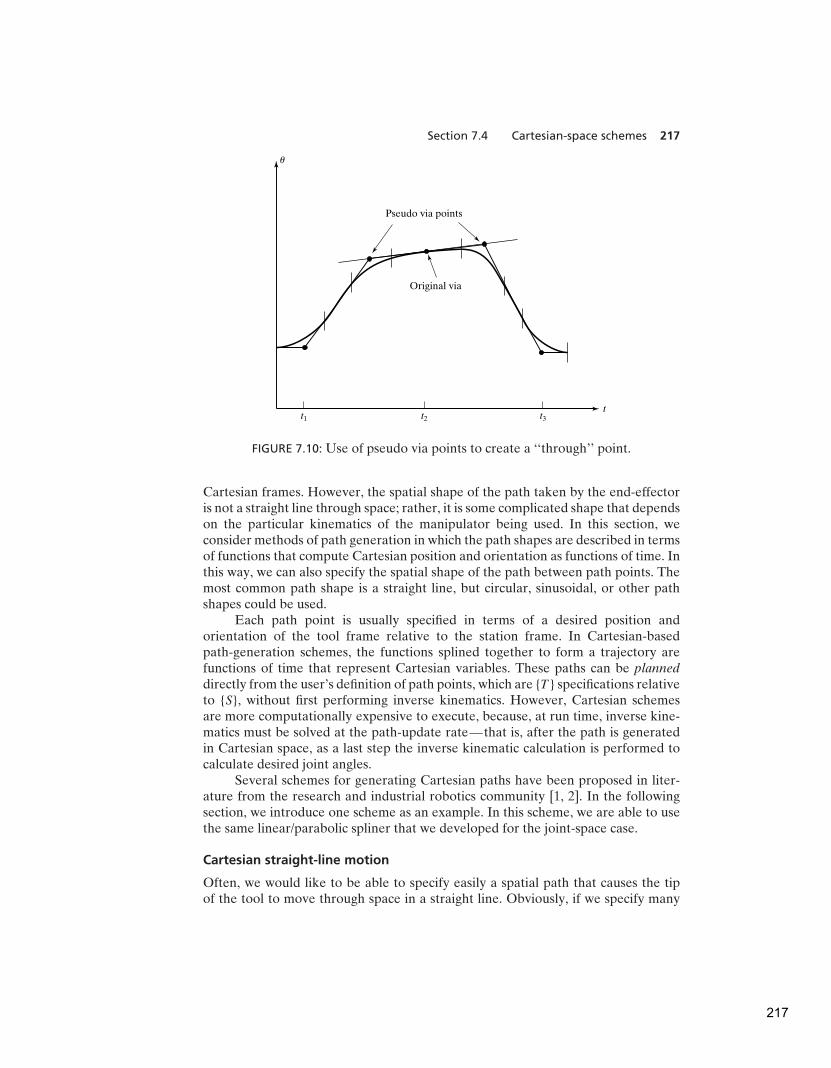
Section 7.4 Cartesian-space schemes 217
u
Pseudo via points
Original via
tt1 t2 t3
FIGURE 7.10: Use of pseudo via points to create a ‘‘through’’ point.
Cartesian frames. However, the spatial shape of the path taken by the end-effectoris not a straight line through space; rather, it is some complicated shape that dependson the particular kinematics of the manipulator being used. In this section, weconsider methods of path generation in which the path shapes are described in termsof functions that compute Cartesian position and orientation as functions of time. Inthis way, we can also specify the spatial shape of the path between path points. Themost common path shape is a straight line, but circular, sinusoidal, or other pathshapes could be used.
Each path point is usually specified in terms of a desired position andorientation of the tool frame relative to the station frame. In Cartesian-basedpath-generation schemes, the functions splined together to form a trajectory arefunctions of time that represent Cartesian variables. These paths can be planned
directly from the user’s definition of path points, which are {T } specifications relativeto {S}, without first performing inverse kinematics. However, Cartesian schemesare more computationally expensive to execute, because, at run time, inverse kine-matics must be solved at the path-update rate—that is, after the path is generatedin Cartesian space, as a last step the inverse kinematic calculation is performed tocalculate desired joint angles.
Several schemes for generating Cartesian paths have been proposed in liter-ature from the research and industrial robotics community [1, 2]. In the followingsection, we introduce one scheme as an example. In this scheme, we are able to usethe same linear/parabolic spliner that we developed for the joint-space case.
Cartesian straight-line motion
Often, we would like to be able to specify easily a spatial path that causes the tipof the tool to move through space in a straight line. Obviously, if we specify many
217
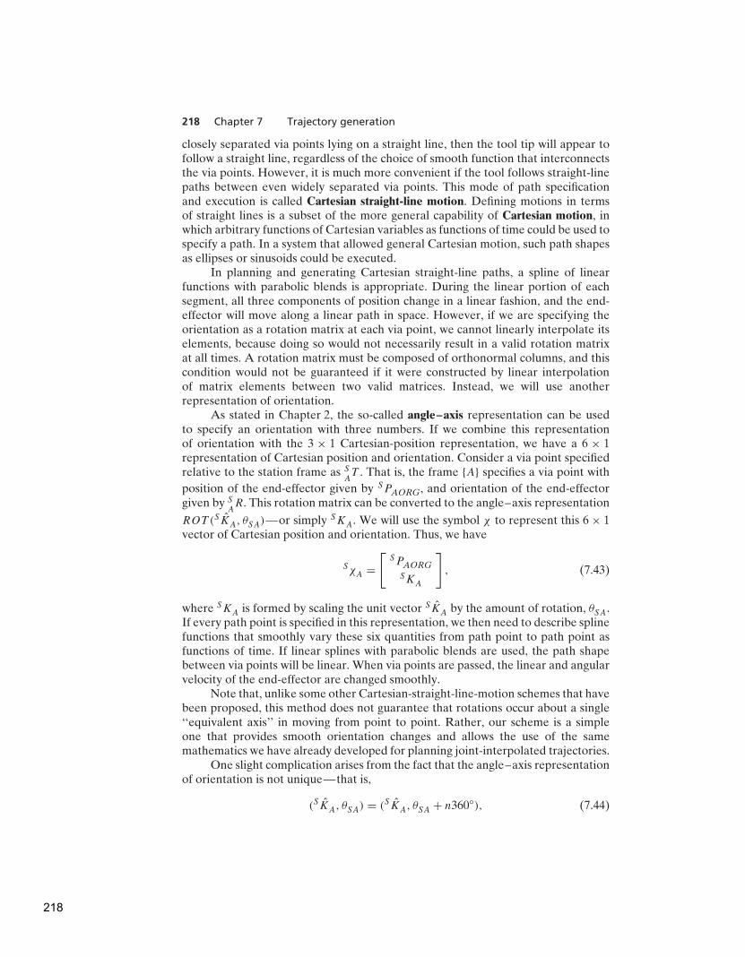
218 Chapter 7 Trajectory generation
closely separated via points lying on a straight line, then the tool tip will appear tofollow a straight line, regardless of the choice of smooth function that interconnectsthe via points. However, it is much more convenient if the tool follows straight-linepaths between even widely separated via points. This mode of path specificationand execution is called Cartesian straight-line motion. Defining motions in termsof straight lines is a subset of the more general capability of Cartesian motion, inwhich arbitrary functions of Cartesian variables as functions of time could be used tospecify a path. In a system that allowed general Cartesian motion, such path shapesas ellipses or sinusoids could be executed.
In planning and generating Cartesian straight-line paths, a spline of linearfunctions with parabolic blends is appropriate. During the linear portion of eachsegment, all three components of position change in a linear fashion, and the end-effector will move along a linear path in space. However, if we are specifying theorientation as a rotation matrix at each via point, we cannot linearly interpolate itselements, because doing so would not necessarily result in a valid rotation matrixat all times. A rotation matrix must be composed of orthonormal columns, and thiscondition would not be guaranteed if it were constructed by linear interpolationof matrix elements between two valid matrices. Instead, we will use anotherrepresentation of orientation.
As stated in Chapter 2, the so-called angle–axis representation can be usedto specify an orientation with three numbers. If we combine this representationof orientation with the 3 × 1 Cartesian-position representation, we have a 6 × 1representation of Cartesian position and orientation. Consider a via point specifiedrelative to the station frame as S
AT . That is, the frame {A} specifies a via point with
position of the end-effector given by SPAORG, and orientation of the end-effectorgiven by S
AR. This rotation matrix can be converted to the angle–axis representation
ROT (SKA, θSA)—or simply SKA. We will use the symbol χ to represent this 6 × 1vector of Cartesian position and orientation. Thus, we have
SχA =
[
SPAORGSKA
]
, (7.43)
where SKA is formed by scaling the unit vector SKA by the amount of rotation, θSA.If every path point is specified in this representation, we then need to describe splinefunctions that smoothly vary these six quantities from path point to path point asfunctions of time. If linear splines with parabolic blends are used, the path shapebetween via points will be linear. When via points are passed, the linear and angularvelocity of the end-effector are changed smoothly.
Note that, unlike some other Cartesian-straight-line-motion schemes that havebeen proposed, this method does not guarantee that rotations occur about a single‘‘equivalent axis’’ in moving from point to point. Rather, our scheme is a simpleone that provides smooth orientation changes and allows the use of the samemathematics we have already developed for planning joint-interpolated trajectories.
One slight complication arises from the fact that the angle–axis representationof orientation is not unique—that is,
(SKA, θSA) = (SKA, θSA + n360◦), (7.44)
218

Section 7.5 Geometric problems with Cartesian paths 219
SKA
SKB(0)
SKB(�1)
SKB(�2)
SKB(1)
SKB(�1) � SKA
FIGURE 7.11: Choosing angle–axis representation to minimize rotation.
where n is any positive or negative integer. In going from a via point {A} to a viapoint {B}, the total amount of rotation should be minimized. If our representationof the orientation of {A} is given as SKA, we must choose the particular SKB suchthat |SKB −S KA| is minimized. For example, Fig. 7.11 shows four different possibleSKB ’s and their relation to the given SKA. The difference vectors (broken lines)are compared to learn which SKB which will result in minimum rotation—in thiscase, SKB(−1).
Once we select the six values of χ for each via point, we can use the samemathematics we have already developed for generating splines that are composed oflinear and parabolic sections. However, we must add one more constraint: The blendtimes for each degree of freedom must be the same. This will ensure that the resultantmotion of all the degrees of freedom will be a straight line in space. Because all blendtimes must be the same, the acceleration used during the blend for each degree offreedom will differ. Hence, we specify a duration of blend, and, using (7.24), wecompute the needed acceleration (instead of the other way around). The blend timecan be chosen so that a certain upper bound on acceleration is not exceeded.
Many other schemes for representing and interpolating the orientation portionof a Cartesian path can be used. Among these are the use of some of the other3 × 1 representations of orientation introduced in Section 2.8. For example, someindustrial robots move along Cartesian straight-line paths in which interpolation oforientation is done by means of a representation similar to Z–Y–Z Euler angles.
7.5 GEOMETRIC PROBLEMS WITH CARTESIAN PATHS
Because a continuous correspondence is made between a path shape described inCartesian space and joint positions, Cartesian paths are prone to various problemsrelating to workspace and singularities.
219

220 Chapter 7 Trajectory generation
B
A
FIGURE 7.12: Cartesian-path problem of type 1.
Problems of type 1: intermediate points unreachable
Although the initial location of the manipulator and the final goal point are bothwithin the manipulator workspace, it is quite possible that not all points lying ona straight line connecting these two points are in the workspace. As an example,consider the planar two-link robot shown in Fig. 7.12 and its associated workspace.In this case, link 2 is shorter than link 1, so the workspace contains a hole in themiddle whose radius is the difference between link lengths. Drawn on the workspaceis a start point A and a goal point B. Moving from A to B would be no problemin joint space, but if a Cartesian straight-line motion were attempted, intermediatepoints along the path would not be reachable. This is an example of a situation inwhich a joint-space path could easily be executed, but a Cartesian straight-line pathwould fail.2
Problems of type 2: high joint rates near singularity
We saw in Chapter 5 that there are locations in the manipulator’s workspacewhere it is impossible to choose finite joint rates that yield the desired velocityof the end-effector in Cartesian space. It should not be surprising, therefore, thatthere are certain paths (described in Cartesian terms) which are impossible for themanipulator to perform. If, for example, a manipulator is following a Cartesianstraight-line path and approaches a singular configuration of the mechanism, oneor more joint velocities might increase toward infinity. Because velocities of the
2Some robot systems would notify the user of a problem before moving the manipulator; in others,motion would start along the path until some joint reaches its limit, at which time manipulator motionwould be halted.
220

Section 7.5 Geometric problems with Cartesian paths 221
A
B
FIGURE 7.13: Cartesian-path problem of type 2.
mechanism are upper bounded, this situation usually results in the manipulator’sdeviating from the desired path.
As an example, Fig. 7.13 shows a planar two-link (with equal link lengths)moving along a path from point A to point B. The desired trajectory is to move theend tip of the manipulator at constant linear velocity along the straight-line path.In the figure, several intermediate positions of the manipulator have been drawn tohelp visualize its motion. All points along the path are reachable, but as the robotgoes past the middle portion of the path, the velocity of joint one is very high. Thecloser the path comes to the joint-one axis, the faster this rate will be. One approachis to scale down the overall velocity of the path to a speed where all joints stay withintheir velocity capabilities. In this way, the desired temporal attributes of the pathmight be lost, but at least the spatial aspect of the trajectory definition is adhered to.
Problems of type 3: start and goal reachable in different solutions
A third kind of problem that could arise is shown in Fig. 7.14. Here, a planar two-linkwith equal link lengths has joint limits that restrict the number of solutions withwhich it can reach a given point in space. In particular, a problem will arise if thegoal point cannot be reached in the same physical solution as the robot is in at thestart point. In Fig. 7.14, the manipulator can reach all points of the path in somesolution, but not in any one solution. In this situation, the manipulator trajectoryplanning system can detect this problem without ever attempting to move the robotalong the path and can signal an error to the user.
To handle these problems with paths specified in Cartesian space, mostindustrial manipulator-control systems support both joint-space and Cartesian-space
221
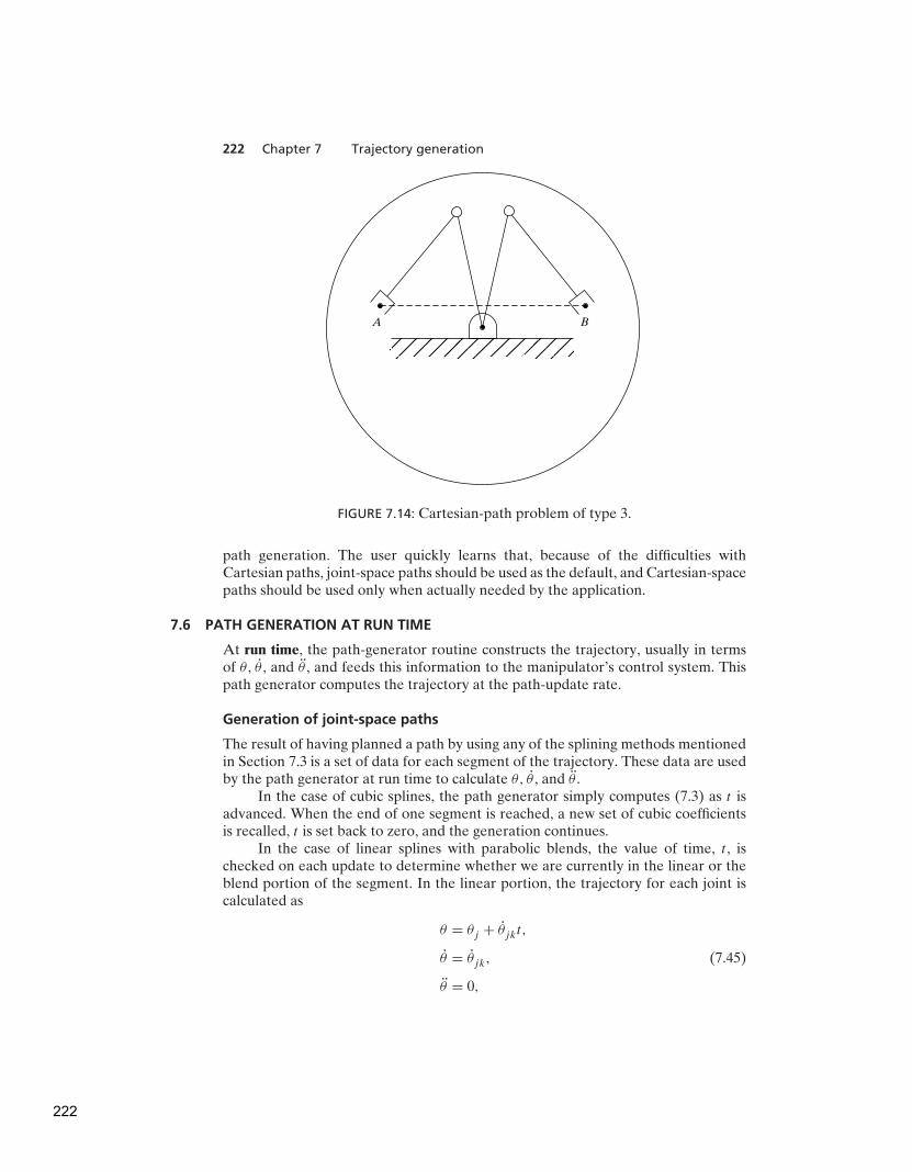
222 Chapter 7 Trajectory generation
A B
FIGURE 7.14: Cartesian-path problem of type 3.
path generation. The user quickly learns that, because of the difficulties withCartesian paths, joint-space paths should be used as the default, and Cartesian-spacepaths should be used only when actually needed by the application.
7.6 PATH GENERATION AT RUN TIME
At run time, the path-generator routine constructs the trajectory, usually in termsof θ, θ , and θ , and feeds this information to the manipulator’s control system. Thispath generator computes the trajectory at the path-update rate.
Generation of joint-space paths
The result of having planned a path by using any of the splining methods mentionedin Section 7.3 is a set of data for each segment of the trajectory. These data are usedby the path generator at run time to calculate θ, θ , and θ .
In the case of cubic splines, the path generator simply computes (7.3) as t isadvanced. When the end of one segment is reached, a new set of cubic coefficientsis recalled, t is set back to zero, and the generation continues.
In the case of linear splines with parabolic blends, the value of time, t , ischecked on each update to determine whether we are currently in the linear or theblend portion of the segment. In the linear portion, the trajectory for each joint iscalculated as
θ = θj + θjkt,
θ = θjk, (7.45)
θ = 0,
222
Section 7.6 Path generation at run time 223
where t is the time since the j th via point and θjk was calculated at path-planningtime from (7.24). In the blend region, the trajectory for each joint is calculated as
tinb = t − ( 12 tj + tjk),
θ = θj + θjk(t − tinb)+ 12 θkt
2inb, (7.46)
θ = θjk + θktinb,
θ = θk,
where θjk, θk, tj , and tjk were calculated at path-planning time by equations (7.24)
through (7.28). This continues, with t being reset to 12 tk when a new linear segment
is entered, until we have worked our way through all the data sets representing thepath segments.
Generation of Cartesian-space paths
For the Cartesian-path scheme presented in Section 7.4, we use the path generatorfor the linear spline with parabolic blends path. However, the values computedrepresent the Cartesian position and orientation rather than joint-variable values,so we rewrite (7.45) and (7.46) with the symbol x representing a component of theCartesian position and orientation vector. In the linear portion of the segment, eachdegree of freedom in χ is calculated as
x = xj + xjkt,
x = xjk, (7.47)
x = 0,
where t is the time since the j th via point and xjk was calculated at path-planningtime by using an equation analogous to (7.24). In the blend region, the trajectoryfor each degree of freedom is calculated as
tinb = t − ( 12 tj + tjk),
x = xj + xjk(t − tinb)+ 12 xkt
2inb, (7.48)
x = xjk + xktinb,
x = xk,
where the quantities xjk, xk, tj , and tjk were computed at plan time, just as in thejoint-space case.
Finally, this Cartesian trajectory (χ, χ , and χ) must be converted into equiva-lent joint-space quantities. A complete analytical solution to this problem would usethe inverse kinematics to calculate joint positions, the inverse Jacobian for velocities,and the inverse Jacobian plus its derivative for accelerations [5]. A simpler way oftenused in practice is as follows: At the path-update rate, we convert χ into its equiv-alent frame representation, S
GT . We then use the SOLVE routine (see Section 4.8)
to calculate the required vector of joint angles, �. Numerical differentiation is then
223

224 Chapter 7 Trajectory generation
used to compute � and �.3 Thus, the algorithm is
χ → S
GT ,
�(t) = SOLVE(SGT ),
�(t) =�(t)−�(t − δt)
δt, (7.49)
�(t) =�(t)− �(t − δt)
δt.
Then �, �, and � are supplied to the manipulator’s control system.
7.7 DESCRIPTION OF PATHS WITH A ROBOT PROGRAMMING LANGUAGE
In Chapter 12, we will discuss robot programming languages further. Here, we willillustrate how various types of paths that we have discussed in this chapter might bespecified in a robot language. In these examples, we use the syntax of AL, a robotprogramming language developed at Stanford University [6].
The symbols A, B, C, and D stand for variables of type ‘‘frame’’ in theAL-language examples that follow. These frames specify path points that we willassume to have been taught or textually described to the system. Assume that themanipulator begins in position A. To move the manipulator in joint-space modealong linear-parabolic-blend paths, we could say
move ARM to C with duration = 3*seconds;
To move to the same position and orientation in a straight line we could saymove ARM to C linearly with duration = 3*seconds;
where the keyword ‘‘linearly’’ denotes that Cartesian straight-line motion is to beused. If duration is not important, the user can omit this specification, and the systemwill use a default velocity—that is,
move ARM to C;
A via point can be added, and we can writemove ARM to C via B;
or a whole set of via points might be specified bymove ARM to C via B,A,D;
Note that inmove ARM to C via B with duration = 6*seconds;
the duration is given for the entire motion. The system decides how to split thisduration between the two segments. It is possible in AL to specify the duration of asingle segment—for example, by
move ARM to C via B where duration = 3*seconds;
The first segment which leads to point B will have a duration of 3 seconds.
7.8 PLANNING PATHS WHEN USING THE DYNAMIC MODEL
Usually, when paths are planned, we use a default or a maximum acceleration at eachblend point. Actually, the amount of acceleration that the manipulator is capable
3This differentiation can be done noncausally for preplanned paths, resulting in better-quality � and�. Also, many control systems do not require a � input, and so it would not be computed.
224
Bibliography 225
of at any instant is a function of the dynamics of the arm and the actuator limits.Most actuators are not characterized by a fixed maximum torque or acceleration,but rather by a torque–speed curve.
When we plan a path assuming there is a maximum acceleration at each jointor along each degree of freedom, we are making a tremendous simplification. Inorder to be careful not to exceed the actual capabilities of the device, this maximumacceleration must be chosen conservatively. Therefore, we are not making fulluse of the speed capabilities of the manipulator in paths planned by the methodsintroduced in this chapter.
We might ask the following question: Given a desired spatial path of theend-effector, find the timing information (which turns a description of a spatial pathinto a trajectory) such that the manipulator reaches the goal point in minimum time.Such problems have been solved by numerical means [7, 8]. The solution takes boththe rigid-body dynamics and actuator speed–torque constraint curves into account.
7.9 COLLISION-FREE PATH PLANNING
It would be extremely convenient if we could simply tell the robot system whatthe desired goal point of the manipulator motion is and let the system determinewhere and how many via points are required so that the goal is reached withoutthe manipulator’s hitting any obstacles. In order to do this, the system must havemodels of the manipulator, the work area, and all potential obstacles in the area. Asecond manipulator could even be working in the same area; in that case, each armwould have to be considered a moving obstacle for the other.
Systems that plan collision-free paths are not available commercially. Researchin this area has led to two competing principal techniques and to several varia-tions and combinations thereof. One approach solves the problem by forming aconnected-graph representation of the free space and then searching the graph for acollision-free path [9–11, 17, 18]. Unfortunately, these techniques have exponentialcomplexity in the number of joints in the device. The second approach is based oncreating artificial potential fields around obstacles, which cause the manipulator(s)to avoid the obstacles while they are drawn toward an artificial attractive pole atthe goal point [12]. Unfortunately, these methods generally have a local view of theenvironment and are subject to becoming ‘‘stuck’’ at local minima of the artificialfield.
BIBLIOGRAPHY
[1] R.P. Paul and H. Zong, ‘‘Robot Motion Trajectory Specification and Generation,’’2nd International Symposium on Robotics Research, Kyoto, Japan, August 1984.
[2] R. Taylor, ‘‘Planning and Execution of Straight Line Manipulator Trajectories,’’ inRobot Motion, Brady et al., Editors, MIT Press, Cambridge, MA, 1983.
[3] C. DeBoor, A Practical Guide to Splines, Springer-Verlag, New York, 1978.
[4] D. Rogers and J.A. Adams, Mathematical Elements for Computer Graphics, McGraw-Hill, New York, 1976.
[5] B. Gorla and M. Renaud, Robots Manipulateurs, Cepadues-Editions, Toulouse, 1984.
[6] R. Goldman, Design of an Interactive Manipulator Programming Environment, UMIResearch Press, Ann Arbor, MI, 1985.
225
226 Chapter 7 Trajectory generation
[7] J. Bobrow, S. Dubowsky, and J. Gibson, ‘‘On the Optimal Control of Robotic Manip-ulators with Actuator Constraints,’’ Proceedings of the American Control Conference,June 1983.
[8] K. Shin and N. McKay, ‘‘Minimum-Time Control of Robotic Manipulators with Geo-metric Path Constraints,’’ IEEE Transactions on Automatic Control, June 1985.
[9] T. Lozano-Perez, ‘‘Spatial Planning: A Configuration Space Approach,’’ AI Memo605, MIT Artificial Intelligence Laboratory, Cambridge, MA, 1980.
[10] T. Lozano-Perez, ‘‘A Simple Motion Planning Algorithm for General Robot Manip-ulators,’’ IEEE Journal of Robotics and Automation, Vol. RA-3, No. 3, June 1987.
[11] R. Brooks, ‘‘Solving the Find-Path Problem by Good Representation of Free Space,’’IEEE Transactions on Systems, Man, and Cybernetics, SMC-13:190–197, 1983.
[12] O. Khatib, ‘‘Real-Time Obstacle Avoidance for Manipulators and Mobile Robots,’’The International Journal of Robotics Research, Vol. 5, No. 1, Spring 1986.
[13] R.P. Paul, ‘‘Robot Manipulators: Mathematics, Programming, and Control,’’ MITPress, Cambridge, MA, 1981.
[14] R. Castain and R.P. Paul, ‘‘An Online Dynamic Trajectory Generator,’’ The Interna-
tional Journal of Robotics Research, Vol. 3, 1984.
[15] C.S. Lin and P.R. Chang, ‘‘Joint Trajectory of Mechanical Manipulators for CartesianPath Approximation,’’ IEEE Transactions on Systems, Man, and Cybernetics, Vol.SMC-13, 1983.
[16] C.S. Lin, P.R. Chang, and J.Y.S. Luh, ‘‘Formulation and Optimization of Cubic Poly-nomial Joint Trajectories for Industrial Robots,’’ IEEE Transactions on Automatic
Control, Vol. AC-28, 1983.
[17] L. Kavraki, P. Svestka, J.C. Latombe, and M. Overmars, ‘‘Probabilistic Roadmaps forPath Planning in High-Dimensional Configuration Spaces,’’ IEEE Transactions on
Robotics and Automation, 12(4): 566–580, 1996.
[18] J. Barraquand, L. Kavraki, J.C. Latombe, T.Y. Li, R. Motwani, and P. Raghavan,‘‘A Random Sampling Scheme for Path Planning,’’ International Journal of Robotics
Research, 16(6): 759–774, 1997.
EXERCISES
7.1 [8] How many individual cubics are computed when a six-jointed robot movesalong a cubic spline path through two via points and stops at a goal point? Howmany coefficients are stored to describe these cubics?
7.2 [13] A single-link robot with a rotary joint is motionless at θ = −5◦. It is desired tomove the joint in a smooth manner to θ = 80◦ in 4 seconds. Find the coefficientsof a cubic which accomplishes this motion and brings the arm to rest at the goal.Plot the position, velocity, and acceleration of the joint as a function of time.
7.3 [14] A single-link robot with a rotary joint is motionless at θ = −5◦. It is desiredto move the joint in a smooth manner to θ = 80◦ in 4 seconds and stop smoothly.Compute the corresponding parameters of a linear trajectory with parabolicblends. Plot the position, velocity, and acceleration of the joint as a function oftime.
7.4 [30] Write a path-planning software routine that implements (7.24) through (7.28)in a general way for paths described by an arbitrary number of path points. Forexample, this routine could be used to solve Example 7.4.
226
Exercises 227
7.5 [18] Sketch graphs of position, velocity, and acceleration for the two-segmentcontinuous-acceleration spline given in Example 7.2. Sketch them for a joint forwhich θ0 = 5.0◦, θυ = 15.0◦, θg = 40.0◦, and each segment lasts 1.0 second.
7.6 [18] Sketch graphs of position, velocity, and acceleration for a two-segment splinewhere each segment is a cubic, using the coefficients as given in (7.11). Sketchthem for a joint where θ0 = 5.0◦ for the initial point, θυ = 15.0◦ is a via point,and θg = 40.0◦ is the goal point. Assume that each segment has a duration of 1.0second and that the velocity at the via point is to be 17.5 degrees/second.
7.7 [20] Calculate θ12, θ23, t1, t2, and t3 for a two-segment linear spline with parabolicblends. (Use (7.24) through (7.28).) For this joint, θ1 = 5.0◦, θ2 = 15.0◦, θ3 = 40.0◦.Assume that td12 = td23 = 1.0 second and that the default acceleration to use
during blends is 80 degrees/second2. Sketch plots of position, velocity, andacceleration of θ .
7.8 [18] Sketch graphs of position, velocity, and acceleration for the two-segmentcontinuous-acceleration spline given in Example 7.2. Sketch them for a joint forwhich θ0 = 5.0◦, θv = 15.0◦, θg = −10.0◦, and each segment lasts 2.0 seconds.
7.9 [18] Sketch graphs of position, velocity, and acceleration for a two-segment splinewhere each segment is a cubic, using the coefficients as given in (7.11). Sketchthem for a joint where θ0 = 5.0◦ for the initial point, θv = 15.0◦ is a via point,and θg = −10.0◦ is the goal point. Assume that each segment has a duration of2.0 seconds and that the velocity at the via point is to be 0.0 degrees/second.
7.10 [20] Calculate θ12, θ23, t1, t2, and t3 for a two-segment linear spline with parabolicblends. (Use (7.24) through (7.28).) For this joint, θ1 = 5.0◦, θ2 = 15.0◦, θ3 =−10.0◦. Assume that td12 = td23 = 2.0 seconds and that the default acceleration
to use during blends is 60 degrees/second2. Sketch plots of position, velocity, andacceleration of θ .
7.11 [6] Give the 6 × 1 Cartesian position and orientation representation sχG that is
equivalent to SGT where S
GR = ROT (Z, 30◦) and SPGORG = [10.0 20.0 30.0]T .
7.12 [6] Give the SGT that is equivalent to the 6 × 1 Cartesian position and orientation
representation SχG = [5.0 −20.0 10.0 45.0 0.0 0.0]T .7.13 [30] Write a program that uses the dynamic equations from Section 6.7 (the
two-link planar manipulator) to compute the time history of torques needed tomove the arm along the trajectory of Exercise 7.8. What are the maximum torquesrequired and where do they occur along the trajectory?
7.14 [32] Write a program that uses the dynamic equations from Section 6.7 (thetwo-link planar manipulator) to compute the time history of torques needed tomove the arm along the trajectory of Exercise 7.8. Make separate plots of thejoint torques required due to inertia, velocity terms, and gravity.
7.15 [22] Do Example 7.2 when tf 1 �= tf 2.7.16 [25] We wish to move a single joint from θ0 to θf starting from rest, ending at rest,
in time tf . The values of θ0 and θf are given, but we wish to compute tf so that
‖θ (t)‖ < θmax and ‖θ (t)‖ < θmax for all t , where θmax and θmax are given positiveconstants. Use a single cubic segment, and give an expression for tf and for thecubic’s coefficients.
7.17 [10] A single cubic trajectory is given by
θ(t) = 10 + 90t2 − 60t3
and is used over the time interval from t = 0 to t = 1. What are the starting andfinal positions, velocities, and accelerations?
227
228 Chapter 7 Trajectory generation
7.18 [12] A single cubic trajectory is given by
θ(t) = 10 + 90t2 − 60t3
and is used over the time interval from t = 0 to t = 2. What are the starting andfinal positions, velocities, and accelerations?
7.19 [13] A single cubic trajectory is given by
θ(t) = 10 + 5t + 70t2 − 45t3
and is used over the time interval from t = 0 to t = 1. What are the starting andfinal positions, velocities, and accelerations?
7.20 [15] A single cubic trajectory is given by
θ(t) = 10 + 5t + 70t2 − 45t3
and is used over the time interval from t = 0 to t = 2. What are the starting andfinal positions, velocities, and accelerations?
PROGRAMMING EXERCISE (PART 7)
1. Write a joint-space, cubic-splined path-planning system. One routine that yoursystem should include is
Procedure CUBCOEF (VAR thO, thf, thdotO, thdotf: real; VAR cc:
vec4);
where
th0 = initial position of θ at beginning of segment,
thf = final position of θ at segment end,
thdot0 = initial velocity of segment,
thdotf = final velocity of segment.
These four quantities are inputs, and ‘‘cc’’, an array of the four cubic coefficients,is the output.
Your program should accept up to (at least) five via-point specifications—in theform of tool frame, {T }, relative to station frame, {S}—in the usual user form:(x, y, φ). To keep life simple, all segments will have the same duration. Your systemshould solve for the coefficients of the cubics, using some reasonable heuristic forassigning joint velocities at the via points. Hint: See option 2 in Section 7.3.
2. Write a path-generator system that calculates a trajectory in joint space basedon sets of cubic coefficients for each segment. It must be able to generate themultisegment path you planned in Problem 1. A duration for the segments willbe specified by the user. It should produce position, velocity, and accelerationinformation at the path-update rate, which will also be specified by the user.
3. The manipulator is the same three-link used previously. The definitions of the {T }and {S} frames are the same as before:
W
TT = [x y θ] = [0.1 0.2 30.0],
B
ST = [x y θ] = [0.0 0.0 0.0].
228
MATLAB Exercise 7 229
Using a duration of 3.0 seconds per segment, plan and execute the path that startswith the manipulator at position
[x1 y1 φ1] = [0.758 0.173 0.0],
moves through the via points
[x2 y2 φ2] = [0.6 −0.3 45.0]
and[x3 y3 φ3] = [−0.4 0.3 120.0],
and ends at the goal point (in this case, same as initial point)
[x4 y4 φ4] = [0.758 0.173 0.0].
Use a path-update rate of 40 Hz, but print the position only every 0.2 seconds.Print the positions out in terms of Cartesian user form. You don’t have to printout velocities or accelerations, though you might be interested in doing so.
MATLAB EXERCISE 7
The goal of this exercise is to implement polynomial joint-space trajectory-generationequations for a single joint. (Multiple joints would require n applications of the result.)Write a MATLAB program to implement the joint-space trajectory generation forthe three cases that follow. Report your results for the specific assignments given; foreach case, give the polynomial functions for the joint angle, angular velocity, angularacceleration, and angular jerk (the time derivative of acceleration). For each case, plotthe results. (Arrange the plots vertically with angle, velocity, acceleration, and then jerk,all with the same time scale—check out the subplot MATLAB function to accomplishthis.) Don’t just plot out results—give some discussion; do your results make sense?Here are the three cases:
a) Third-order polynomial. Force the angular velocity to be zero at the start and atthe finish. Given θs = 120
◦(start), θf = 60
◦(finish), and tf = 1 sec.
b) Fifth-order polynomial. Force the angular velocity and acceleration to be zero atthe start and at the finish. Given θs = 120
◦, θf = 60
◦, and tf = 1 sec. Compare your
results (functions and plots) with this same example, but using a single third-orderpolynomial, as in problem (a).
c) Two third-order polynomials with via point. Force the angular velocity to bezero at the start and at the finish. Don’t force the angular velocity to be zeroat the via point—you must match velocity and acceleration at this point for thetwo polynomials meeting at that point in time. Demonstrate that this conditionis satisfied. Given θs = 60
◦(start), θv = 120
◦(via), θf = 30
◦(finish), and
t1 = t2 = 1 sec (relative time steps—i.e., tf = 2 sec).
d) Check the results of (a) and (b) by means of the Corke MATLAB RoboticsToolbox. Try function jtraj().
229
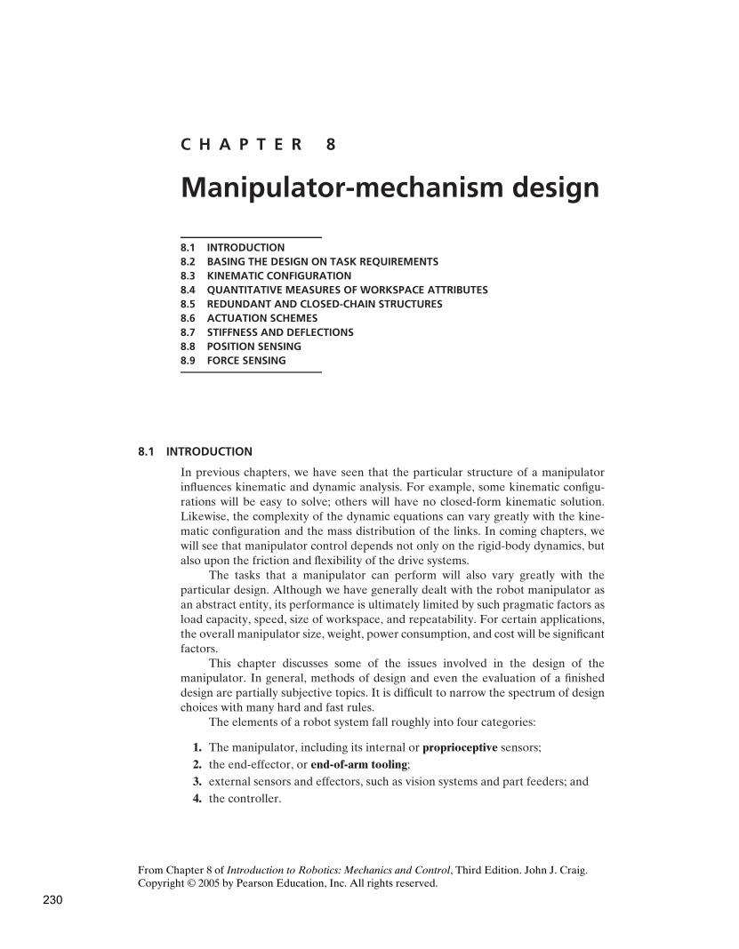
C H A P T E R 8
Manipulator-mechanism design
8.1 INTRODUCTION
8.2 BASING THE DESIGN ON TASK REQUIREMENTS
8.3 KINEMATIC CONFIGURATION
8.4 QUANTITATIVE MEASURES OF WORKSPACE ATTRIBUTES
8.5 REDUNDANT AND CLOSED-CHAIN STRUCTURES
8.6 ACTUATION SCHEMES
8.7 STIFFNESS AND DEFLECTIONS
8.8 POSITION SENSING
8.9 FORCE SENSING
8.1 INTRODUCTION
In previous chapters, we have seen that the particular structure of a manipulatorinfluences kinematic and dynamic analysis. For example, some kinematic configu-rations will be easy to solve; others will have no closed-form kinematic solution.Likewise, the complexity of the dynamic equations can vary greatly with the kine-matic configuration and the mass distribution of the links. In coming chapters, wewill see that manipulator control depends not only on the rigid-body dynamics, butalso upon the friction and flexibility of the drive systems.
The tasks that a manipulator can perform will also vary greatly with theparticular design. Although we have generally dealt with the robot manipulator asan abstract entity, its performance is ultimately limited by such pragmatic factors asload capacity, speed, size of workspace, and repeatability. For certain applications,the overall manipulator size, weight, power consumption, and cost will be significantfactors.
This chapter discusses some of the issues involved in the design of themanipulator. In general, methods of design and even the evaluation of a finisheddesign are partially subjective topics. It is difficult to narrow the spectrum of designchoices with many hard and fast rules.
The elements of a robot system fall roughly into four categories:
1. The manipulator, including its internal or proprioceptive sensors;
2. the end-effector, or end-of-arm tooling;
3. external sensors and effectors, such as vision systems and part feeders; and
4. the controller.
From Chapter 8 of Introduction to Robotics: Mechanics and Control, Third Edition. John J. Craig.
Copyright © 2005 by Pearson Education, Inc. All rights reserved.
230
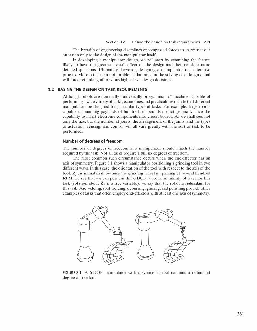
Section 8.2 Basing the design on task requirements 231
The breadth of engineering disciplines encompassed forces us to restrict ourattention only to the design of the manipulator itself.
In developing a manipulator design, we will start by examining the factorslikely to have the greatest overall effect on the design and then consider moredetailed questions. Ultimately, however, designing a manipulator is an iterativeprocess. More often than not, problems that arise in the solving of a design detailwill force rethinking of previous higher level design decisions.
8.2 BASING THE DESIGN ON TASK REQUIREMENTS
Although robots are nominally ‘‘universally programmable’’ machines capable ofperforming a wide variety of tasks, economies and practicalities dictate that differentmanipulators be designed for particular types of tasks. For example, large robotscapable of handling payloads of hundreds of pounds do not generally have thecapability to insert electronic components into circuit boards. As we shall see, notonly the size, but the number of joints, the arrangement of the joints, and the typesof actuation, sensing, and control will all vary greatly with the sort of task to beperformed.
Number of degrees of freedom
The number of degrees of freedom in a manipulator should match the numberrequired by the task. Not all tasks require a full six degrees of freedom.
The most common such circumstance occurs when the end-effector has anaxis of symmetry. Figure 8.1 shows a manipulator positioning a grinding tool in twodifferent ways. In this case, the orientation of the tool with respect to the axis of thetool, ZT , is immaterial, because the grinding wheel is spinning at several hundredRPM. To say that we can position this 6-DOF robot in an infinity of ways for thistask (rotation about ZT is a free variable), we say that the robot is redundant forthis task. Arc welding, spot welding, deburring, glueing, and polishing provide otherexamples of tasks that often employ end-effectors with at least one axis of symmetry.
FIGURE 8.1: A 6-DOF manipulator with a symmetric tool contains a redundantdegree of freedom.
231
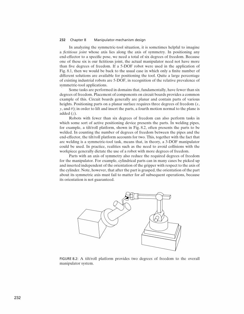
232 Chapter 8 Manipulator-mechanism design
In analyzing the symmetric-tool situation, it is sometimes helpful to imaginea fictitious joint whose axis lies along the axis of symmetry. In positioning anyend-effector to a specific pose, we need a total of six degrees of freedom. Becauseone of these six is our fictitious joint, the actual manipulator need not have morethan five degrees of freedom. If a 5-DOF robot were used in the application ofFig. 8.1, then we would be back to the usual case in which only a finite number ofdifferent solutions are available for positioning the tool. Quite a large percentageof existing industrial robots are 5-DOF, in recognition of the relative prevalence ofsymmetric-tool applications.
Some tasks are performed in domains that, fundamentally, have fewer than sixdegrees of freedom. Placement of components on circuit boards provides a commonexample of this. Circuit boards generally are planar and contain parts of variousheights. Positioning parts on a planar surface requires three degrees of freedom (x,y, and θ); in order to lift and insert the parts, a fourth motion normal to the plane isadded (z).
Robots with fewer than six degrees of freedom can also perform tasks inwhich some sort of active positioning device presents the parts. In welding pipes,for example, a tilt/roll platform, shown in Fig. 8.2, often presents the parts to bewelded. In counting the number of degrees of freedom between the pipes and theend-effector, the tilt/roll platform accounts for two. This, together with the fact thatarc welding is a symmetric-tool task, means that, in theory, a 3-DOF manipulatorcould be used. In practice, realities such as the need to avoid collisions with theworkpiece generally dictate the use of a robot with more degrees of freedom.
Parts with an axis of symmetry also reduce the required degrees of freedomfor the manipulator. For example, cylindrical parts can in many cases be picked upand inserted independent of the orientation of the gripper with respect to the axis ofthe cylinder. Note, however, that after the part is grasped, the orientation of the partabout its symmetric axis must fail to matter for all subsequent operations, becauseits orientation is not guaranteed.
FIGURE 8.2: A tilt/roll platform provides two degrees of freedom to the overallmanipulator system.
232

Section 8.2 Basing the design on task requirements 233
Workspace
In performing tasks, a manipulator has to reach a number of workpieces or fixtures.In some cases, these can be positioned as needed to suit the workspace of themanipulator. In other cases, a robot can be installed in a fixed environment withrigid workspace requirements. Workspace is also sometimes called work volume orwork envelope.
The overall scale of the task sets the required workspace of the manipulator. Insome cases, the details of the shape of the workspace and the location of workspacesingularities will be important considerations.
The intrusion of the manipulator itself in the workspace can sometimesbe a factor. Depending on the kinematic design, operating a manipulator in agiven application could require more or less space around the fixtures in orderto avoid collisions. Restricted environments can affect the choice of kinematicconfiguration.
Load capacity
The load capacity of a manipulator depends upon the sizing of its structuralmembers, power-transmission system, and actuators. The load placed on actuatorsand drive system is a function of the configuration of the robot, the percentage oftime supporting a load, and dynamic loading due to inertial- and velocity-relatedforces.
Speed
An obvious goal in design has been for faster and faster manipulators. Highspeed offers advantages in many applications when a proposed robotic solutionmust compete on economic terms with hard automation or human workers.For some applications, however, the process itself limits the speed rather thanthe manipulator. This is the case with many welding and spray-painting applica-tions.
An important distinction is that between the maximum end-effector speedand the overall cycle time for a particular task. For pick-and-place applications, themanipulator must accelerate and decelerate to and from the pick and place locationswithin some positional accuracy bounds. Often, the acceleration and decelerationphases take up most of the cycle time. Hence, acceleration capability, not just peakspeed, is very important.
Repeatability and accuracy
High repeatability and accuracy, although desirable in any manipulator design, areexpensive to achieve. For example, it would be absurd to design a paint-sprayingrobot to be accurate to within 0.001 inches when the spray spot diameter is 8 inches±2 inches. To a large extent, accuracy of a particular model of industrial robotdepends upon the details of its manufacture rather than on its design. High accuracyis achieved by having good knowledge of the link (and other) parameters. Makingit possible are accurate measurements after manufacture or careful attention totolerances during manufacturing.
233
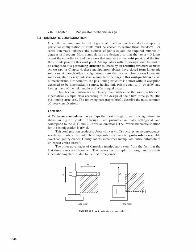
234 Chapter 8 Manipulator-mechanism design
8.3 KINEMATIC CONFIGURATION
Once the required number of degrees of freedom has been decided upon, aparticular configuration of joints must be chosen to realize those freedoms. Forserial kinematic linkages, the number of joints equals the required number ofdegrees of freedom. Most manipulators are designed so that the last n − 3 jointsorient the end-effector and have axes that intersect at the wrist point, and the firstthree joints position this wrist point. Manipulators with this design could be said tobe composed of a positioning structure followed by an orienting structure or wrist.As we saw in Chapter 4, these manipulators always have closed-form kinematicsolutions. Although other configurations exist that possess closed-form kinematicsolutions, almost every industrial manipulator belongs to this wrist-partitioned classof mechanisms. Furthermore, the positioning structure is almost without exceptiondesigned to be kinematically simple, having link twists equal to 0◦ or ±90◦ andhaving many of the link lengths and offsets equal to zero.
It has become customary to classify manipulators of the wrist-partitioned,kinematically simple class according to the design of their first three joints (thepositioning structure). The following paragraphs briefly describe the most commonof these classifications.
Cartesian
A Cartesian manipulator has perhaps the most straightforward configuration. Asshown in Fig. 8.3, joints 1 through 3 are prismatic, mutually orthogonal, andcorrespond to the X, Y , and Z Cartesian directions. The inverse kinematic solutionfor this configuration is trivial.
This configuration produces robots with very stiff structures. As a consequence,very large robots can be built. These large robots, often called gantry robots, resembleoverhead gantry cranes. Gantry robots sometimes manipulate entire automobilesor inspect entire aircraft.
The other advantages of Cartesian manipulators stem from the fact that thefirst three joints are decoupled. This makes them simpler to design and preventskinematic singularities due to the first three joints.
Side view Top view
d2 d1
d3
FIGURE 8.3: A Cartesian manipulator.
234

Section 8.3 Kinematic configuration 235
Their primary disadvantage is that all of the feeders and fixtures associated withan application must lie ‘‘inside’’ the robot. Consequently, application workcells forCartesian robots become very machine dependent. The size of the robot’s supportstructure limits the size and placement of fixtures and sensors. These limitationsmake retrofitting Cartesian robots into existing workcells extremely difficult.
Articulated
Figure 8.4 shows an articulated manipulator, sometimes also called a jointed, elbow,or anthropomorphic manipulator. A manipulator of this kind typically consists oftwo ‘‘shoulder’’ joints (one for rotation about a vertical axis and one for elevationout of the horizontal plane), an ‘‘elbow’’ joint (whose axis is usually parallel to theshoulder elevation joint), and two or three wrist joints at the end of the manipulator.Both the PUMA 560 and the Motoman L-3, which we studied in earlier chapters,fall into this class.
Articulated robots minimize the intrusion of the manipulator structure intothe workspace, making them capable of reaching into confined spaces. They requiremuch less overall structure than Cartesian robots, making them less expensive forapplications needing smaller workspaces.
SCARA
The SCARA1 configuration, shown in Fig. 8.5, has three parallel revolute joints(allowing it to move and orient in a plane), with a fourth prismatic joint for movingthe end-effector normal to the plane. The chief advantage is that the first threejoints don’t have to support any of the weight of the manipulator or the load. Inaddition, link 0 can easily house the actuators for the first two joints. The actuatorscan be made very large, so the robot can move very fast. For example, the Adept
Top viewSide view
u1u3
u2
FIGURE 8.4: An articulated manipulator.
1SCARA stands for ‘‘selectively compliant assembly robot arm.’’
235
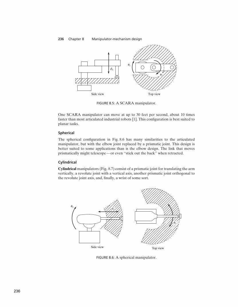
236 Chapter 8 Manipulator-mechanism design
Side view Top view
d3
u1
u2
FIGURE 8.5: A SCARA manipulator.
One SCARA manipulator can move at up to 30 feet per second, about 10 timesfaster than most articulated industrial robots [1]. This configuration is best suited toplanar tasks.
Spherical
The spherical configuration in Fig. 8.6 has many similarities to the articulatedmanipulator, but with the elbow joint replaced by a prismatic joint. This design isbetter suited to some applications than is the elbow design. The link that movesprismatically might telescope—or even ‘‘stick out the back’’ when retracted.
Cylindrical
Cylindrical manipulators (Fig. 8.7) consist of a prismatic joint for translating the armvertically, a revolute joint with a vertical axis, another prismatic joint orthogonal tothe revolute joint axis, and, finally, a wrist of some sort.
u2d3
Side view Top view
u1
FIGURE 8.6: A spherical manipulator.
236
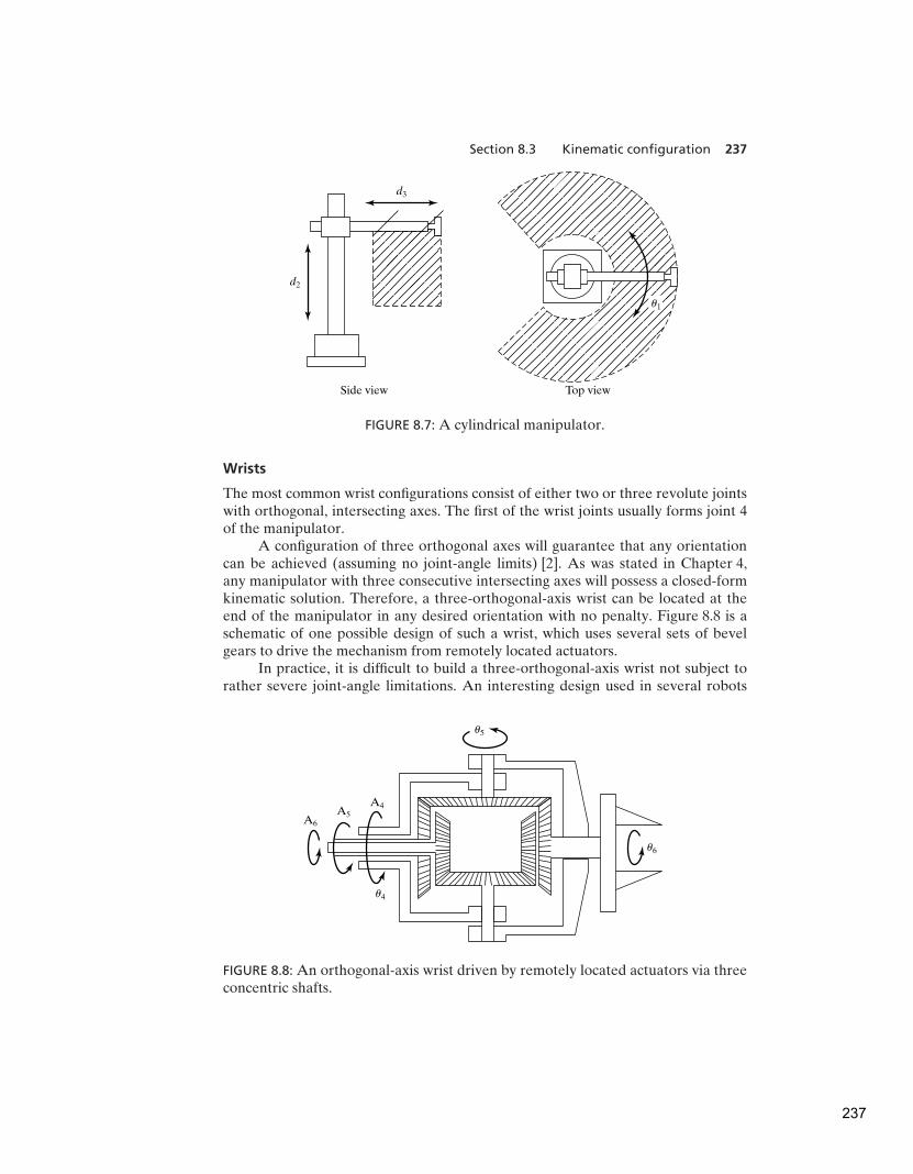
Section 8.3 Kinematic configuration 237
d3
d2
Side view Top view
u1
FIGURE 8.7: A cylindrical manipulator.
Wrists
The most common wrist configurations consist of either two or three revolute jointswith orthogonal, intersecting axes. The first of the wrist joints usually forms joint 4of the manipulator.
A configuration of three orthogonal axes will guarantee that any orientationcan be achieved (assuming no joint-angle limits) [2]. As was stated in Chapter 4,any manipulator with three consecutive intersecting axes will possess a closed-formkinematic solution. Therefore, a three-orthogonal-axis wrist can be located at theend of the manipulator in any desired orientation with no penalty. Figure 8.8 is aschematic of one possible design of such a wrist, which uses several sets of bevelgears to drive the mechanism from remotely located actuators.
In practice, it is difficult to build a three-orthogonal-axis wrist not subject torather severe joint-angle limitations. An interesting design used in several robots
A6
A5
A4
u4
u5
u6
FIGURE 8.8: An orthogonal-axis wrist driven by remotely located actuators via threeconcentric shafts.
237

238 Chapter 8 Manipulator-mechanism design
manufactured by Cincinatti Milacron (Fig. 1.4) employs a wrist that has threeintersecting but nonorthogonal axes. In this design (called the ‘‘three roll wrist’’), allthree joints of the wrist can rotate continuously without limits. The nonorthogonalityof the axes creates, however, a set of orientations that are impossible to reach withthis wrist. This set of unattainable orientations is described by a cone within whichthe third axis of the wrist cannot lie. (See Exercise 8.11.) However, the wrist can bemounted to link 3 of the manipulator in such a way that the link structure occupiesthis cone and so would be block access anyway. Figure 8.9 shows two drawings ofsuch a wrist [24].
Some industrial robots have wrists that do not have intersecting axes. Thisimplies that a closed-form kinematic solution might not exist. If, however, the wrist ismounted on an articulated manipulator in such a way that the joint-4 axis is parallelto the joint-2 and -3 axes, as in Fig. 8.10, there will be a closed-form kinematicsolution. Likewise, a nonintersecting-axis wrist mounted on a Cartesian robot yieldsa closed-form-solvable manipulator.
Typically, 5-DOF welding robots use two-axis wrists oriented as shown inFig. 8.11. Note that, if the robot has a symmetric tool, this ‘‘fictitious joint’’ mustfollow the rules of wrist design. That is, in order to reach all orientations, the toolmust be mounted with its axis of symmetry orthogonal to the joint-5 axis. In theworst case, when the axis of symmetry is parallel to the joint-5 axis, the fictitioussixth axis is in a permanently singular configuration.
u4
u5
u6
u6
u5
u4
(a)
(b)
FIGURE 8.9: Two views of a nonorthogonal-axis wrist [24]. From International Ency-
clopedia of Robotics, by R. Dorf and S. Nof (editors). From ‘‘Wrists’’ by M. Rosheim,John C. Wiley and Sons, Inc., New York, NY 1988. Reprinted by permission.
238

Section 8.4 Quantitative measures of workspace attributes 239
u1
u2
u3
u4
u6
u5
FIGURE 8.10: A manipulator with a wrist whose axes do not intersect. However, thisrobot does possess a closed-form kinematic solution.
u4
u5
TZ
FIGURE 8.11: Typical wrist design of a 5-DOF welding robot.
8.4 QUANTITATIVE MEASURES OF WORKSPACE ATTRIBUTES
Manipulator designers have proposed several interesting quantitative measures of
various workspace attributes.
239
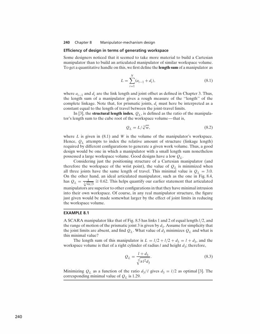
240 Chapter 8 Manipulator-mechanism design
Efficiency of design in terms of generating workspace
Some designers noticed that it seemed to take more material to build a Cartesianmanipulator than to build an articulated manipulator of similar workspace volume.To get a quantitative handle on this, we first define the length sum of a manipulator as
L =N
∑
i=1
(ai−1 + di), (8.1)
where ai−1 and di are the link length and joint offset as defined in Chapter 3. Thus,the length sum of a manipulator gives a rough measure of the ‘‘length’’ of thecomplete linkage. Note that, for prismatic joints, di must here be interpreted as aconstant equal to the length of travel between the joint-travel limits.
In [3], the structural length index, QL, is defined as the ratio of the manipula-tor’s length sum to the cube root of the workspace volume—that is,
QL = L/ 3√w, (8.2)
where L is given in (8.1) and W is the volume of the manipulator’s workspace.Hence, QL attempts to index the relative amount of structure (linkage length)required by different configurations to generate a given work volume. Thus, a gooddesign would be one in which a manipulator with a small length sum nonethelesspossessed a large workspace volume. Good designs have a low QL.
Considering just the positioning structure of a Cartesian manipulator (andtherefore the workspace of the wrist point), the value of QL is minimized whenall three joints have the same length of travel. This minimal value is QL = 3.0.On the other hand, an ideal articulated manipulator, such as the one in Fig. 8.4,has QL = 1
3√
4π/3∼= 0.62. This helps quantify our earlier statement that articulated
manipulators are superior to other configurations in that they have minimal intrusioninto their own workspace. Of course, in any real manipulator structure, the figurejust given would be made somewhat larger by the effect of joint limits in reducingthe workspace volume.
EXAMPLE 8.1
A SCARA manipulator like that of Fig. 8.5 has links 1 and 2 of equal length l/2, andthe range of motion of the prismatic joint 3 is given by d3. Assume for simplicity thatthe joint limits are absent, and find QL. What value of d3 minimizes QL and what isthis minimal value?
The length sum of this manipulator is L = l/2 + l/2 + d3 = l + d3, and theworkspace volume is that of a right cylinder of radius l and height d3; therefore,
QL = l + d3
3
√
πl2d3
. (8.3)
Minimizing QL as a function of the ratio d3/l gives d3 = l/2 as optimal [3]. Thecorresponding minimal value of QL is 1.29.
240

Section 8.5 Redundant and closed-chain structures 241
Designing well-conditioned workspaces
At singular points, a manipulator effectively loses one or more degrees of free-dom, so certain tasks may not be able to be performed at that point. In fact, inthe neighborhood of singular points (including workspace-boundary singularities),actions of the manipulator could fail to be well-conditioned. In some sense, thefarther the manipulator is away from singularities, the better able it is to moveuniformly and apply forces uniformly in all directions. Several measures have beensuggested for quantifying this effect. The use of such measures at design time mightyield a manipulator design with a maximally large well-conditioned subspace of theworkspace.
Singular configurations are given by
det(J (�)) = 0, (8.4)
so it is natural to use the determinant of the Jacobian in a measure of manipulatordexterity. In [4], the manipulability measure, w, is defined as
w =√
det(J (�)J T (�)), (8.5)
which, for a nonredundant manipulator, reduces to
w = |det(J (�))|. (8.6)
A good manipulator design has large areas of its workspace characterized by highvalues of w.
Whereas velocity analysis motivated (8.6), other researchers have proposedmanipulability measures based on acceleration analysis or force-application capa-bility. Asada [5] suggested an examination of the eigenvalues of the Cartesian massmatrix
Mx(�) = J−T (�)M(�)J−1(�) (8.7)
as a measure of how well the manipulator can accelerate in various Cartesiandirections. He suggests a graphic representation of this measure as an inertiaellipsoid, given by
XTMx(�)X = 1, (8.8)
the equation of an n-dimensional ellipse, where n is the dimension of X. The axes ofthe ellipsoid given in (8.8) lie in the directions of the eigenvectors of Mx(�), and thereciprocals of the square roots of the corresponding eigenvalues provide the lengthsof the axes of the ellipsoid. Well-conditioned points in the manipulator workspaceare characterized by inertia ellipsoids that are spherical (or nearly so).
Figure 8.12 shows graphically the properties of a planar two-link manipulator.In the center of the workspace, the manipulator is well conditioned, as is indicatedby nearly circular ellipsoids. At workspace boundaries, the ellipses flatten, indicatingthe manipulator’s difficulty in accelerating in certain directions.
Other measures of workspace conditioning have been proposed in [6–8, 25].
8.5 REDUNDANT AND CLOSED-CHAIN STRUCTURES
In general, the scope of this book is limited to manipulators that are serial-chain linkages of six or fewer joints. In this section, however, we briefly discussmanipulators outside of this class.
241

242 Chapter 8 Manipulator-mechanism design
FIGURE 8.12: Workspace of a 2-DOF planar arm, showing inertia ellipsoids, from [5]( 1984 IEEE). The dashed line indicates a locus of isotropic points in the workspace.Reprinted by permission.
Micromanipulators and other redundancies
General spatial positioning capability requires only six degrees of freedom, but thereare advantages to having even more controllable joints.
One use for these extra freedoms is already finding some practical applica-tion [9,10] and is of growing interest in the research community: a micromanipulator.A micromanipulator is generally formed by several fast, precise degrees of freedomlocated near the distal end of a ‘‘conventional’’ manipulator. The conventionalmanipulator takes care of large motions, while the micromanipulator, whose jointsgenerally have a small range of motion, accomplishes fine motion and force control.
Additional joints can also help a mechanism avoid singular configurations,as is suggested in [11, 12]. For example, any three-degree-of-freedom wrist willsuffer from singular configurations (when all three axes lie in a plane), but afour-degree-of-freedom wrist can effectively avoid such configurations [13–15].
Figure 8.13 shows two configurations suggested [11, 12] for seven-degree-of-freedom manipulators.
A major potential use of redundant robots is in avoiding collisions whileoperating in cluttered work environments. As we have seen, a six-degree-of-freedommanipulator can reach a given position and orientation in only a finite number ofways. The addition of a seventh joint allows an infinity of ways, permitting the desireto avoid obstacles to influence the choice.
Closed-loop structures
Although we have considered only serial-chain manipulators in our analysis, somemanipulators contain closed-loop structures. For example, the Motoman L-3 robotdescribed in Chapters 3 and 4 possesses closed-loop structures in the drive mecha-nism of joints 2 and 3. Closed-loop structures offer a benefit: increased stiffness of
242

Section 8.5 Redundant and closed-chain structures 243
u1
u2
u3
u4
u5u6
u7
u1
u2
u4
u6
u3 u5
u7
FIGURE 8.13: Two suggested seven-degree-of-freedom manipulator designs [3].
the mechanism [16]. On the other hand, closed-loop structures generally reduce theallowable range of motion of the joints and thus decrease the workspace size.
Figure 8.14 depicts a Stewart mechanism, a closed-loop alternative to the serial6-DOF manipulator. The position and orientation of the ‘‘end-effector’’ is controlledby the lengths of the six linear actuators which connect it to the base. At the base end,each actuator is connected by a two-degree-of-freedom universal joint. At the end-effector, each actuator is attached with a three-degree-of-freedom ball-and-socketjoint. It exhibits characteristics common to most closed-loop mechanisms: it can bemade very stiff, but the links have a much more limited range of motion than doserial linkages. The Stewart mechanism, in particular, demonstrates an interestingreversal in the nature of the forward and inverse kinematic solutions: the inversesolution is quite simple, whereas the forward solution is typically quite complex,sometimes lacking a closed-form formulation. (See Exercises 8.7 and 8.12.)
In general, the number of degrees of freedom of a closed-loop mechanism isnot obvious. The total number of degrees of freedom can be computed by means ofGrubler’s formula [17],
F = 6(l − n − 1) +n
∑
i=1
fi, (8.9)
where F is the total number of degrees of freedom in the mechanism, l is thenumber of links (including the base), n is the total number of joints, and fi is thenumber of degrees of freedom associated with the ith joint. A planar version ofGrubler’s formula (when all objects are considered to have three degrees of freedomif unconstrained) is obtained by replacing the 6 in (8.9) with a 3.
243

244 Chapter 8 Manipulator-mechanism design
d5
d6
d4
d3
d2
d1
Base
�End-effector �
FIGURE 8.14: The Stewart mechanism is a six-degree-of-freedom fully parallel manip-ulator.
EXAMPLE 8.2
Use Grubler’s formula to verify that the Stewart mechanism (Fig. 8.14) indeed hassix degrees of freedom.
The number of joints is 18 (6 universal, 6 ball and socket, and 6 prismatic inthe actuators). The number of links is 14 (2 parts for each actuator, the end-effector,and the base). The sum of all the joint freedoms is 36. Using Grubler’s formula, wecan verify that the total number of degrees of freedom is six:
F = 6(14 − 18 − 1) + 36 = 6. (8.10)
8.6 ACTUATION SCHEMES
Once the general kinematic structure of a manipulator has been chosen, the nextmost important matter of concern is the actuation of the joints. Typically, theactuator, reduction, and transmission are closely coupled and must be designedtogether.
Actuator location
The most straightforward choice of actuator location is at or near the joint it drives.If the actuator can produce enough torque or force, its output can attach directlyto the joint. This arrangement, known as a direct-drive configuration [18], offers
244
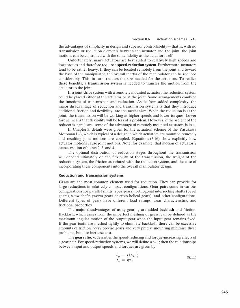
Section 8.6 Actuation schemes 245
the advantages of simplicity in design and superior controllability—that is, with notransmission or reduction elements between the actuator and the joint, the jointmotions can be controlled with the same fidelity as the actuator itself.
Unfortunately, many actuators are best suited to relatively high speeds andlow torques and therefore require a speed-reduction system. Furthermore, actuatorstend to be rather heavy. If they can be located remotely from the joint and towardthe base of the manipulator, the overall inertia of the manipulator can be reducedconsiderably. This, in turn, reduces the size needed for the actuators. To realizethese benefits, a transmission system is needed to transfer the motion from theactuator to the joint.
In a joint-drive system with a remotely mounted actuator, the reduction systemcould be placed either at the actuator or at the joint. Some arrangements combinethe functions of transmission and reduction. Aside from added complexity, themajor disadvantage of reduction and transmission systems is that they introduceadditional friction and flexibility into the mechanism. When the reduction is at thejoint, the transmission will be working at higher speeds and lower torques. Lowertorque means that flexibility will be less of a problem. However, if the weight of thereducer is significant, some of the advantage of remotely mounted actuators is lost.
In Chapter 3, details were given for the actuation scheme of the YasukawaMotoman L-3, which is typical of a design in which actuators are mounted remotelyand resulting joint motions are coupled. Equations (3.16) show explicitly howactuator motions cause joint motions. Note, for example, that motion of actuator 2causes motion of joints 2, 3, and 4.
The optimal distribution of reduction stages throughout the transmissionwill depend ultimately on the flexibility of the transmission, the weight of thereduction system, the friction associated with the reduction system, and the ease ofincorporating these components into the overall manipulator design.
Reduction and transmission systems
Gears are the most common element used for reduction. They can provide forlarge reductions in relatively compact configurations. Gear pairs come in variousconfigurations for parallel shafts (spur gears), orthogonal intersecting shafts (bevelgears), skew shafts (worm gears or cross helical gears), and other configurations.Different types of gears have different load ratings, wear characteristics, andfrictional properties.
The major disadvantages of using gearing are added backlash and friction.Backlash, which arises from the imperfect meshing of gears, can be defined as themaximum angular motion of the output gear when the input gear remains fixed.If the gear teeth are meshed tightly to eliminate backlash, there can be excessiveamounts of friction. Very precise gears and very precise mounting minimize theseproblems, but also increase cost.
The gear ratio, η, describes the speed-reducing and torque-increasing effects ofa gear pair. For speed-reduction systems, we will define η > 1; then the relationshipsbetween input and output speeds and torques are given by
θo = (1/η)θiτo = ητi,
(8.11)
245
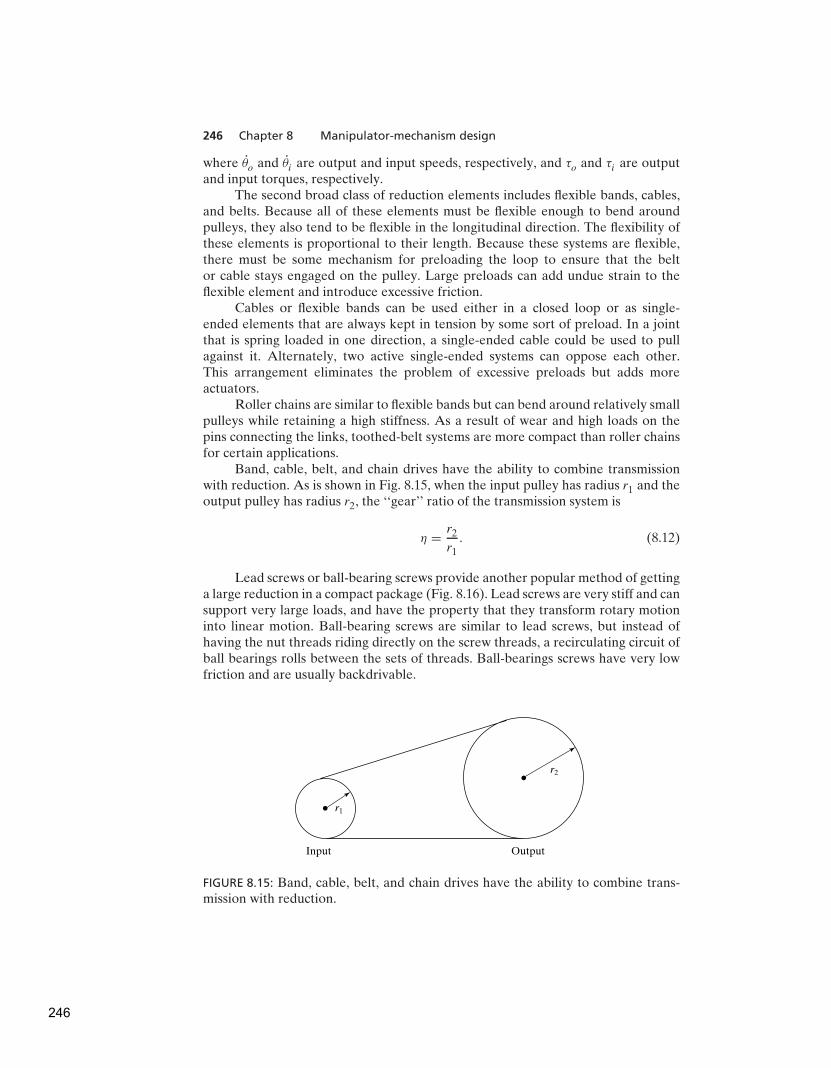
246 Chapter 8 Manipulator-mechanism design
where θo and θi are output and input speeds, respectively, and τo and τi are outputand input torques, respectively.
The second broad class of reduction elements includes flexible bands, cables,and belts. Because all of these elements must be flexible enough to bend aroundpulleys, they also tend to be flexible in the longitudinal direction. The flexibility ofthese elements is proportional to their length. Because these systems are flexible,there must be some mechanism for preloading the loop to ensure that the beltor cable stays engaged on the pulley. Large preloads can add undue strain to theflexible element and introduce excessive friction.
Cables or flexible bands can be used either in a closed loop or as single-ended elements that are always kept in tension by some sort of preload. In a jointthat is spring loaded in one direction, a single-ended cable could be used to pullagainst it. Alternately, two active single-ended systems can oppose each other.This arrangement eliminates the problem of excessive preloads but adds moreactuators.
Roller chains are similar to flexible bands but can bend around relatively smallpulleys while retaining a high stiffness. As a result of wear and high loads on thepins connecting the links, toothed-belt systems are more compact than roller chainsfor certain applications.
Band, cable, belt, and chain drives have the ability to combine transmissionwith reduction. As is shown in Fig. 8.15, when the input pulley has radius r1 and theoutput pulley has radius r2, the ‘‘gear’’ ratio of the transmission system is
η = r2
r1
. (8.12)
Lead screws or ball-bearing screws provide another popular method of gettinga large reduction in a compact package (Fig. 8.16). Lead screws are very stiff and cansupport very large loads, and have the property that they transform rotary motioninto linear motion. Ball-bearing screws are similar to lead screws, but instead ofhaving the nut threads riding directly on the screw threads, a recirculating circuit ofball bearings rolls between the sets of threads. Ball-bearings screws have very lowfriction and are usually backdrivable.
r1
r2
Input Output
FIGURE 8.15: Band, cable, belt, and chain drives have the ability to combine trans-mission with reduction.
246

Section 8.7 Stiffness and deflections 247
Nut
(a) (b)
Race
FIGURE 8.16: Lead screws (a) and ball-bearing screws (b) combine a large reductionand transformation from rotary to linear motion.
8.7 STIFFNESS AND DEFLECTIONS
An important goal for the design of most manipulators is overall stiffness of thestructure and the drive system. Stiff systems provide two main benefits. First,because typical manipulators do not have sensors to measure the tool framelocation directly, it is calculated by using the forward kinematics based on sensedjoint positions. For an accurate calculation, the links cannot sag under gravity orother loads. In other words, we wish our Denavit–Hartenberg description of thelinkages to remain fixed under various loading conditions. Second, flexibilities inthe structure or drive train will lead to resonances, which have an undesirable effecton manipulator performance. In this section, we consider issues of stiffness andthe resulting deflections under loads. We postpone further discussion of resonancesuntil Chapter 9.
Flexible elements in parallel and in series
As can be easily shown (see Exercise 8.21), the combination of two flexible membersof stiffness k1 and k2 ‘‘connected in parallel’’ produces the net stiffness
kparallel = k1 + k2; (8.13)
‘‘connected in series,’’ the combination produces the net stiffness
1
kseries
= 1
k1
+ 1
k2
. (8.14)
In considering transmission systems, we often have the case of one stageof reduction or transmission in series with a following stage of reduction ortransmission; hence, (8.14) becomes useful.
Shafts
A common method for transmitting rotary motion is through shafts. The torsionalstiffness of a round shaft can be calculated [19] as
k = Gπd4
32l, (8.15)
247

248 Chapter 8 Manipulator-mechanism design
where d is the shaft diameter, l is the shaft length, and G is the shear modulus ofelasticity (about 7.5×10¹⁰ Nt/m2 for steel, and about a third as much for aluminum).
Gears
Gears, although typically quite stiff, introduce compliance into the drive system. Anapproximate formula to estimate the stiffness of the output gear (assuming the inputgear is fixed) is given in [20] as
k = Cgbr2, (8.16)
where b is the face width of the gears, r is the radius of the output gear, andCg = 1.34 × 10¹⁰ Nt/m2 for steel.
Gearing also has the effect of changing the effective stiffness of the drivesystem by a factor of η2. If the stiffness of the transmission system prior to thereduction (i.e., on the input side) is ki , so that
τi = kiδθi, (8.17)
and the stiffness of the output side of the reduction is ko, so that
τo = koδθo, (8.18)
then we can compute the relationship between ki and ko (under the assumption of aperfectly rigid gear pair) as
ko = τo
δθo= ηkiδθi
(1/η)δθi= η2ki . (8.19)
Hence, a gear reduction has the effect of increasing the stiffness by the square of thegear ratio.
EXAMPLE 8.3
A shaft with torsional stiffness equal to 500.0 Nt-m/radian is connected to theinput side of a gear set with η = 10, whose output gear (when the input gear isfixed) exhibits a stiffness of 5000.0 Nt m/radian. What is the output stiffness of thecombined drive system?
Using (8.14) and (8.19), we have
1
kseries
= 1
5000.0+ 1
102(500.0), (8.20)
or
kseries = 50000
11∼= 4545.4 Nt m/radian. (8.21)
When a relatively large speed reduction is the last element of a multielementtransmission system, the stiffnesses of the preceding elements can generally beignored.
248

Section 8.7 Stiffness and deflections 249
l
FIGURE 8.17: Simple cantilever beam used to model the stiffness of a link to an endload.
Belts
In such a belt drive as that of Fig. 8.15, stiffness is given by
k = AE
l, (8.22)
where A is the cross-sectional area of the belt, E is the modulus of elasticity of thebelt, and l is the length of the free belt between pulleys plus one-third of the lengthof the belt in contact with the pulleys [19].
Links
As a rough approximation of the stiffness of a link, we might model a single link asa cantilever beam and calculate the stiffness at the end point, as in Fig. 8.17. For around hollow beam, this stiffness is given by [19]
k =3πE(d4
o− d4
i)
64l3, (8.23)
where di and do are the inner and outer diameters of the tubular beam, l is thelength, and E is the modulus of elasticity (about 2 × 10¹¹ Nt/m2 for steel, and abouta third as much for aluminum). For a square-cross-section hollow beam, this stiffnessis given by
k =E(w4
o− w4
i)
4l3, (8.24)
where wi and wo are the outer and inner widths of the beam (i.e., the wall thicknessis wo − wi).
EXAMPLE 8.4
A square-cross-section link of dimensions 5 × 5 × 50 cm with a wall thickness of1 cm is driven by a set of rigid gears with η = 10, and the input of the gears is drivenby a shaft having diameter 0.5 cm and length 30 cm. What deflection is caused by aforce of 100 Nt at the end of the link?
249
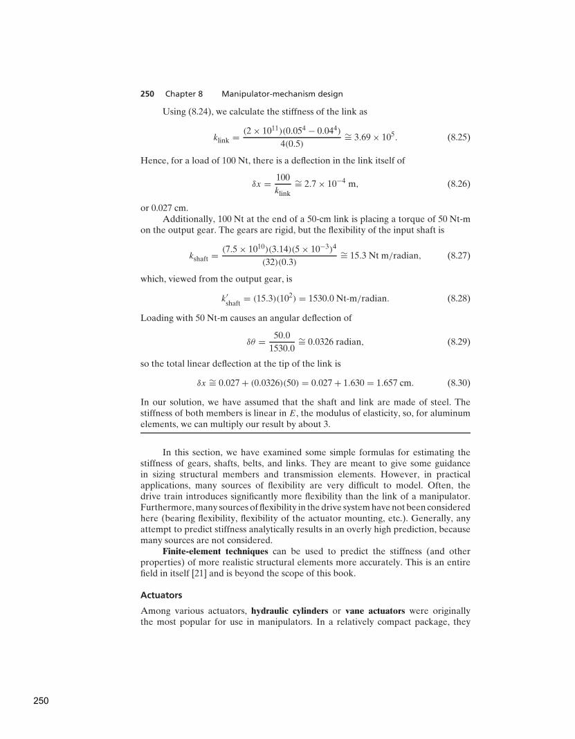
250 Chapter 8 Manipulator-mechanism design
Using (8.24), we calculate the stiffness of the link as
klink = (2 × 10¹¹)(0.054 − 0.044)
4(0.5)∼= 3.69 × 10⁵. (8.25)
Hence, for a load of 100 Nt, there is a deflection in the link itself of
δx = 100
klink
∼= 2.7 × 10⁻⁴ m, (8.26)
or 0.027 cm.Additionally, 100 Nt at the end of a 50-cm link is placing a torque of 50 Nt-m
on the output gear. The gears are rigid, but the flexibility of the input shaft is
kshaft = (7.5 × 10¹⁰)(3.14)(5 × 10⁻³)4
(32)(0.3)∼= 15.3 Nt m/radian, (8.27)
which, viewed from the output gear, is
k′shaft
= (15.3)(102) = 1530.0 Nt-m/radian. (8.28)
Loading with 50 Nt-m causes an angular deflection of
δθ = 50.0
1530.0∼= 0.0326 radian, (8.29)
so the total linear deflection at the tip of the link is
δx ∼= 0.027 + (0.0326)(50) = 0.027 + 1.630 = 1.657 cm. (8.30)
In our solution, we have assumed that the shaft and link are made of steel. Thestiffness of both members is linear in E, the modulus of elasticity, so, for aluminumelements, we can multiply our result by about 3.
In this section, we have examined some simple formulas for estimating thestiffness of gears, shafts, belts, and links. They are meant to give some guidancein sizing structural members and transmission elements. However, in practicalapplications, many sources of flexibility are very difficult to model. Often, thedrive train introduces significantly more flexibility than the link of a manipulator.Furthermore, many sources of flexibility in the drive system have not been consideredhere (bearing flexibility, flexibility of the actuator mounting, etc.). Generally, anyattempt to predict stiffness analytically results in an overly high prediction, becausemany sources are not considered.
Finite-element techniques can be used to predict the stiffness (and otherproperties) of more realistic structural elements more accurately. This is an entirefield in itself [21] and is beyond the scope of this book.
Actuators
Among various actuators, hydraulic cylinders or vane actuators were originallythe most popular for use in manipulators. In a relatively compact package, they
250
Section 8.7 Stiffness and deflections 251
can produce enough force to drive joints without a reduction system. The speed ofoperation depends upon the pump and accumulator system, usually located remotelyfrom the manipulator. The position control of hydraulic systems is well understoodand relatively straightforward. All of the early industrial robots and many modernlarge industrial robots use hydraulic actuators.
Unfortunately, hydraulics require a great deal of equipment, such as pumps,accumulators, hoses, and servo valves. Hydraulic systems also tend to be inherentlymessy, making them unsuitable for some applications. With the advent of moreadvanced robot-control strategies, in which actuator forces must be applied accu-rately, hydraulics proved disadvantageous, because of the friction contributed bytheir seals.
Pneumatic cylinders possess all the favorable attributes of hydraulics, andthey are cleaner than hydraulics—air seeps out instead of hydraulic fluid. However,pneumatic actuators have proven difficult to control accurately, because of thecompressibility of air and the high friction of the seals.
Electric motors are the most popular actuator for manipulators. Althoughthey don’t have the power-to-weight ratio of hydraulics or pneumatics, their con-trollability and ease of interface makes them attractive for small-to-medium-sizedmanipulators.
Direct current (DC) brush motors (Fig. 8.18) are the most straightforwardto interface and control. The current is conducted to the windings of the rotorvia brushes, which make contact with the revolving commutator. Brush wear andfriction can be problems. New magnetic materials have made high peak torquespossible. The limiting factor on the torque output of these motors is the overheating
Brush
Shaft
Bearings
Commutator
Brush
Stator magnet
Stator magnet
Rotor windings
Shaft angle, u
ia
S
N
FIGURE 8.18: DC brush motors are among the actuators occurring most frequently inmanipulator design. Franklin, Powell, Emami-Naeini, Feedback Control of Dynamic
Systems, 1988, Addison-Wesley, Reading, MA. Reprinted with permission.
251

252 Chapter 8 Manipulator-mechanism design
of the windings. For short duty cycles, high torques can be achieved, but only muchlower torques can be sustained over long periods of time.
Brushless motors solve brush wear and friction problems. Here, the windingsremain stationary and the magnetic field piece rotates. A sensor on the rotor detectsthe shaft angle and is then used by external electronics to perform the commutation.Another advantage of brushless motors is that the winding is on the outside, attachedto the motor case, affording it much better cooling. Sustained torque ratings tend tobe somewhat higher than for similar-sized brush motors.
Alternating current (AC) motors and stepper motors have been used infre-quently in industrial robotics. Difficulty of control of the former and low torqueability of the latter have limited their use.
8.8 POSITION SENSING
Virtually all manipulators are servo-controlled mechanisms—that is, the force ortorque command to an actuator is based on the error between the sensed positionof the joint and the desired position. This requires that each joint have some sort ofposition-sensing device.
The most common approach is to locate a position sensor directly on the shaftof the actuator. If the drive train is stiff and has no backlash, the true joint angles canbe calculated from the actuator shaft positions. Such co-located sensor and actuatorpairs are easiest to control.
The most popular position-feedback device is the rotary optical encoder.As the encoder shaft turns, a disk containing a pattern of fine lines interruptsa light beam. A photodetector turns these light pulses into a binary waveform.Typically, there are two such channels, with wave pulse trains 90 degrees outof phase. The shaft angle is determined by counting the number of pulses, andthe direction of rotation is determined by the relative phase of the two squarewaves. Additionally, encoders generally emit an index pulse at one location, whichcan be used to set a home position in order to compute an absolute angularposition.
Resolvers are devices that output two analog signals—one the sine of the shaftangle, the other the cosine. The shaft angle is computed from the relative magnitudeof the two signals. The resolution is a function of the quality of the resolver and theamount of noise picked up in the electronics and cabling. Resolvers are often morereliable than optical encoders, but their resolution is lower. Typically, resolverscannot be placed directly at the joint without additional gearing to improve theresolution.
Potentiometers provide the most straightforward form of position sensing.Connected in a bridge configuration, they produce a voltage proportional to theshaft position. Difficulties with resolution, linearity, and noise susceptibility limittheir use.
Tachometers are sometimes used to provide an analog signal proportional tothe shaft velocity. In the absence of such velocity sensors, the velocity feedbackis derived by taking differences of sensed position over time. This numerical
differentiation can introduce both noise and a time lag. Despite these potentialproblems, most manipulators are without direct velocity sensing.
252
Section 8.9 Force sensing 253
8.9 FORCE SENSING
A variety of devices have been designed to measure forces of contact between amanipulator’s end-effector and the environment that it touches. Most such sensorsmake use of sensing elements called strain gauges, of either the semiconductor or themetal-foil variety. These strain gauges are bonded to a metal structure and producean output proportional to the strain in the metal. In this type of force-sensor design,the issues the designer must address include the following:
1. How many sensors are needed to resolve the desired information?
2. How are the sensors mounted relative to each other on the structure?
3. What structure allows good sensitivity while maintaining stiffness?
4. How can protection against mechanical overload be built into the device?
There are three places where such sensors are usually placed on a manipulator:
1. At the joint actuators. These sensors measure the torque or force output ofthe actuator/reduction itself. These are useful for some control schemes, butusually do not provide good sensing of contact between the end-effector andthe environment.
2. Between the end-effector and last joint of the manipulator. These sensorsare usually referred to as wrist sensors. They are mechanical structuresinstrumented with strain gauges, which can measure the forces and torquesacting on the end-effector. Typically, these sensors are capable of measuringfrom three to six components of the force/torque vector acting on the end-effector.
3. At the ‘‘fingertips’’ of the end-effector. Usually, these force-sensing fingershave built-in strain gauges to measure from one to four components of forceacting at each fingertip.
As an example, Fig. 8.19 is a drawing of the internal structure of a popular styleof wrist-force sensor designed by Scheinman [22]. Bonded to the cross-bar structureof the device are eight pairs of semiconductor strain gauges. Each pair is wired in avoltage-divider arrangement. Each time the wrist is queried, eight analog voltagesare digitized and read into the computer. Calibration schemes have been designedwith which to arrive at a constant 6 × 8 calibration matrix that maps these eightstrain measurements into the force–torque vector, F , acting on the end-effector.The sensed force–torque vector can be transformed to a reference frame of interest,as we saw in Example 5.8.
Force-sensor design issues
Use of strain gauges to measure force relies on measuring the deflection of a stressedflexure. Therefore, one of the primary design trade-offs is between the stiffness andthe sensitivity of the sensor. A stiffer sensor is inherently less sensitive.
The stiffness of the sensor also affects the construction of overload protection.Strain gauges can be damaged by impact loading and therefore must be protectedagainst such overloads. Transducer damage can be prevented by having limit stops,
253

254 Chapter 8 Manipulator-mechanism design
Instrumentedwith straingauges
X
Z
Y
nx
ny
nz
fz
fx
fy
FIGURE 8.19: The internal structure of a typical force-sensing wrist.
which prevent the flexures from deflecting past a certain point. Unfortunately, avery stiff sensor might deflect only a few ten-thousandths of an inch. Manufacturinglimit stops with such small clearances is very difficult. Consequently, for many typesof transducers, a certain amount of flexibility must be built-in in order to makepossible effective limit stops.
Eliminating hysteresis is one of the most cumbersome restrictions in the sensordesign. Most metals used as flexures, if not overstrained, have very little hysteresis.However, bolted, press-fit, or welded joints near the flexure introduce hysteresis.Ideally, the flexure and the material near it are made from a single piece of metal.
It is also important to use differential measurements to increase the linearityand disturbance rejection of torque sensors. Different physical configurations oftransducers can eliminate influences due to temperature effects and off-axis forces.
Foil gauges are relatively durable, but they produce a very small resistancechange at full strain. Eliminating noise in the strain-gauge cabling and amplificationelectronics is of crucial importance for a good dynamic range.
Semiconductor strain gauges are much more susceptible to damage throughoverload. In their favor, they produce a resistance change about seventy times thatof foil gauges for a given strain. This makes the task of signal processing muchsimpler for a given dynamic range.
BIBLIOGRAPHY
[1] W. Rowe, Editor, Robotics Technical Directory 1986, Instrument Society of America,Research Triangle Park, NC, 1986.
[2] R. Vijaykumar and K. Waldron, ‘‘Geometric Optimization of Manipulator Structuresfor Working Volume and Dexterity,’’ International Journal of Robotics Research, Vol.5, No. 2, 1986.
[3] K. Waldron, ‘‘Design of Arms,’’ in The International Encyclopedia of Robotics, R. Dorfand S. Nof, Editors, John Wiley and Sons, New York, 1988.
254
Bibliography 255
[4] T. Yoshikawa, ‘‘Manipulability of Robotic Mechanisms,’’ The International Journal of
Robotics Research, Vol. 4, No. 2, MIT Press, Cambridge, MA, 1985.
[5] H. Asada, ‘‘Dynamic Analysis and Design of Robot Manipulators Using InertiaEllipsoids,’’ Proceedings of the IEEE International Conference on Robotics, Atlanta,March 1984.
[6] J.K. Salisbury and J. Craig, ‘‘Articulated Hands: Force Control and Kinematic Issues,’’The International Journal of Robotics Research, Vol. 1, No. 1, 1982.
[7] O. Khatib and J. Burdick, ‘‘Optimization of Dynamics in Manipulator Design: TheOperational Space Formulation,’’ International Journal of Robotics and Automation,Vol. 2, No. 2, IASTED, 1987.
[8] T. Yoshikawa, ‘‘Dynamic Manipulability of Robot Manipulators,’’ Proceedings of the
IEEE International Conference on Robotics and Automation, St. Louis, March 1985.
[9] J. Trevelyan, P. Kovesi, and M. Ong, ‘‘Motion Control for a Sheep Shearing Robot,’’The 1st International Symposium of Robotics Research, MIT Press, Cambridge, MA,1984.
[10] P. Marchal, J. Cornu, and J. Detriche, ‘‘Self Adaptive Arc Welding Operation byMeans of an Automatic Joint Following System,’’ Proceedings of the 4th Symposium
on Theory and Practice of Robots and Manipulators, Zaburow, Poland, September1981.
[11] J.M. Hollerbach, ‘‘Optimum Kinematic Design for a Seven Degree of FreedomManipulator,’’ Proceedings of the 2nd International Symposium of Robotics Research,Kyoto, Japan, August 1984.
[12] K. Waldron and J. Reidy, ‘‘A Study of Kinematically Redundant Manipulator Struc-ture,’’ Proceedings of the IEEE Robotics and Automation Conference, San Francisco,April 1986.
[13] V. Milenkovic, ‘‘New Nonsingular Robot Wrist Design,’’ Proceedings of the Robots
11 / 17th ISIR Conference, SME, 1987.
[14] E. Rivin, Mechanical Design of Robots, McGraw-Hill, New York, 1988.
[15] T. Yoshikawa, ‘‘Manipulability of Robotic Mechanisms,’’ in Proceedings of the 2nd
International Symposium on Robotics Research, Kyoto, Japan, 1984.
[16] M. Leu, V. Dukowski, and K. Wang, ‘‘An Analytical and Experimental Study of theStiffness of Robot Manipulators with Parallel Mechanisms,’’ in Robotics and Manu-
facturing Automation, M. Donath and M. Leu, Editors, ASME, New York, 1985.
[17] K. Hunt, Kinematic Geometry of Mechanisms, Cambridge University Press, Cam-bridge, MA, 1978.
[18] H. Asada and K. Youcef-Toumi, Design of Direct Drive Manipulators, MIT Press,Cambridge, MA, 1987.
[19] J. Shigley, Mechanical Engineering Design, 3rd edition, McGraw-Hill, New York,1977.
[20] D. Welbourne, ‘‘Fundamental Knowledge of Gear Noise—A Survey,’’ Proceedings
of the Conference on Noise and Vibrations of Engines and Transmissions, Institute ofMechanical Engineers, Cranfield, UK, 1979.
[21] O. Zienkiewicz, The Finite Element Method, 3rd edition, McGraw-Hill, New York,1977.
255

256 Chapter 8 Manipulator-mechanism design
[22] V. Scheinman, ‘‘Design of a Computer Controlled Manipulator,’’ M.S. Thesis,Mechanical Engineering Department, Stanford University, 1969.
[23] K. Lau, N. Dagalakis, and D. Meyers, ‘‘Testing,’’ in The International Encyclopedia of
Robotics, R. Dorf and S. Nof, Editors, John Wiley and Sons, New York, 1988.
[24] M. Roshiem, ‘‘Wrists,’’ in The International Encyclopedia of Robotics, R. Dorf andS. Nof, Editors, John Wiley and Sons, New York, 1988.
[25] A. Bowling and O. Khatib, ‘‘Robot Acceleration Capability: The Actuation Effi-ciency Measure,’’ Proceedings of the IEEE International Conference on Robotics and
Automation, San Francisco, April 2000.
EXERCISES
8.1 [15] A robot is to be used for positioning a laser cutting device. The laser producesa pinpoint, nondivergent beam. For general cutting tasks, how many degrees offreedom does the positioning robot need? Justify your answer.
8.2 [15] Sketch a possible joint configuration for the laser-positioning robot ofExercise 8.1, assuming that it will be used primarily for cutting at odd anglesthrough 1-inch-thick, 8 × 8-foot plates.
8.3 [17] For a spherical robot like that of Fig. 8.6, if joints 1 and 2 have no limits andjoint 3 has lower limit l and upper limit u, find the structural length index, QL, forthe wrist point of this robot.
8.4 [25] A steel shaft of length 30 cm and diameter 0.2 cm drives the input gear of areduction having η = 8. The output gear drives a steel shaft having length 30 cmand diameter 0.3 cm. If the gears introduce no compliance of their own, what isthe overall stiffness of the transmission system?
8.5 [20] In Fig. 8.20, a link is driven through a shaft after a gear reduction. Modelthe link as rigid with mass of 10 Kg located at a point 30 cm from the shaft axis.Assume that the gears are rigid and that the reduction, η, is large. The shaft issteel and must be 30 cm long. If the design specifications call for the center of linkmass to undergo accelerations of 2.0 g, what should the shaft diameter be to limitdynamic deflections to 0.1 radian at the joint angle?
30
h
30
FIGURE 8.20: A link actuated through a shaft after a gear reduction.
256
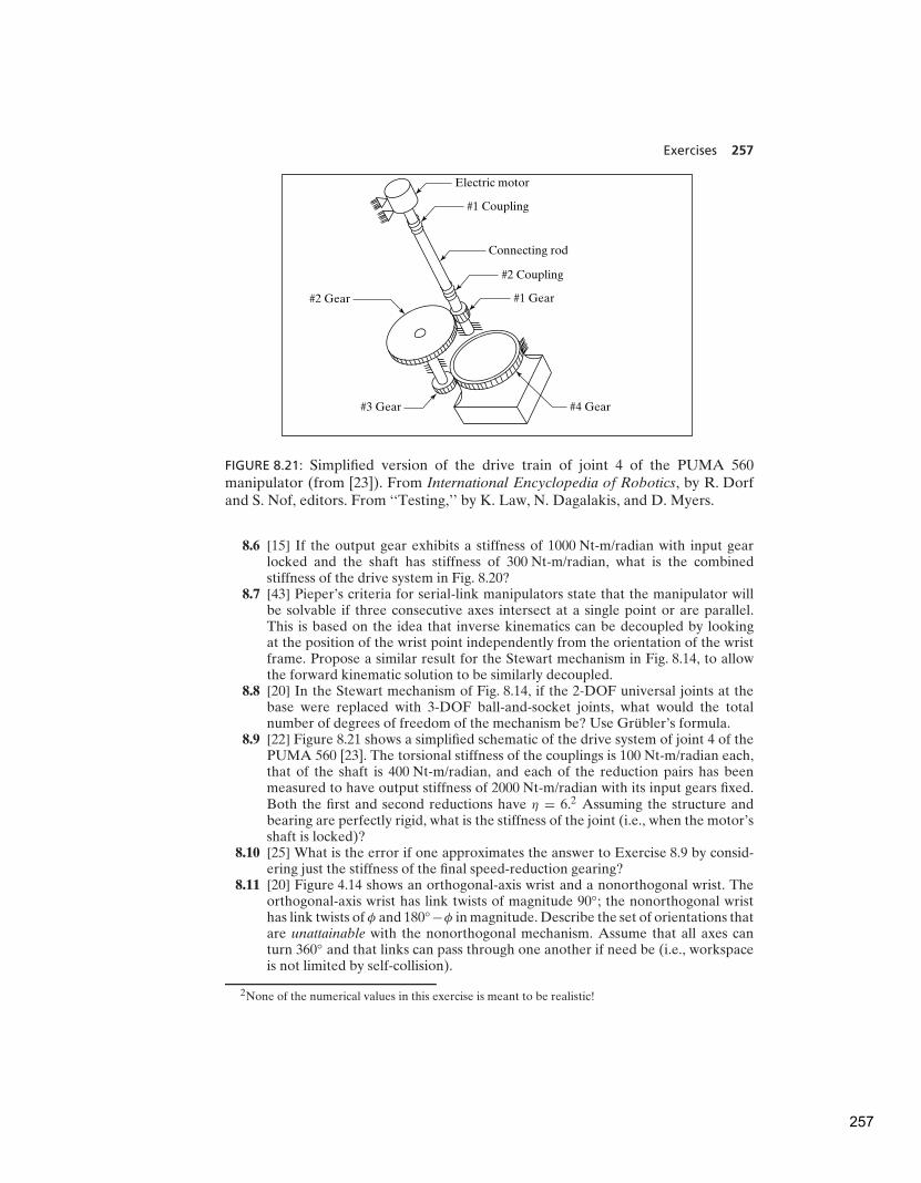
Exercises 257
#3 Gear
#2 Gear
#4 Gear
Connecting rod
#2 Coupling
#1 Coupling
Electric motor
#1 Gear
FIGURE 8.21: Simplified version of the drive train of joint 4 of the PUMA 560manipulator (from [23]). From International Encyclopedia of Robotics, by R. Dorfand S. Nof, editors. From ‘‘Testing,’’ by K. Law, N. Dagalakis, and D. Myers.
8.6 [15] If the output gear exhibits a stiffness of 1000 Nt-m/radian with input gearlocked and the shaft has stiffness of 300 Nt-m/radian, what is the combinedstiffness of the drive system in Fig. 8.20?
8.7 [43] Pieper’s criteria for serial-link manipulators state that the manipulator willbe solvable if three consecutive axes intersect at a single point or are parallel.This is based on the idea that inverse kinematics can be decoupled by lookingat the position of the wrist point independently from the orientation of the wristframe. Propose a similar result for the Stewart mechanism in Fig. 8.14, to allowthe forward kinematic solution to be similarly decoupled.
8.8 [20] In the Stewart mechanism of Fig. 8.14, if the 2-DOF universal joints at thebase were replaced with 3-DOF ball-and-socket joints, what would the totalnumber of degrees of freedom of the mechanism be? Use Grubler’s formula.
8.9 [22] Figure 8.21 shows a simplified schematic of the drive system of joint 4 of thePUMA 560 [23]. The torsional stiffness of the couplings is 100 Nt-m/radian each,that of the shaft is 400 Nt-m/radian, and each of the reduction pairs has beenmeasured to have output stiffness of 2000 Nt-m/radian with its input gears fixed.Both the first and second reductions have η = 6.2 Assuming the structure andbearing are perfectly rigid, what is the stiffness of the joint (i.e., when the motor’sshaft is locked)?
8.10 [25] What is the error if one approximates the answer to Exercise 8.9 by consid-ering just the stiffness of the final speed-reduction gearing?
8.11 [20] Figure 4.14 shows an orthogonal-axis wrist and a nonorthogonal wrist. Theorthogonal-axis wrist has link twists of magnitude 90◦; the nonorthogonal wristhas link twists of φ and 180◦−φ in magnitude. Describe the set of orientations thatare unattainable with the nonorthogonal mechanism. Assume that all axes canturn 360◦ and that links can pass through one another if need be (i.e., workspaceis not limited by self-collision).
2None of the numerical values in this exercise is meant to be realistic!
257

258 Chapter 8 Manipulator-mechanism design
d5
p5
p6
{B}
{T}
p1
p4
q5 q3
q6 q1
q4
q2
p2
p3
d3
FIGURE 8.22: Stewart mechanism of Exercise 8.12.
8.12 [18] Write down a general inverse-kinematic solution for the Stewart mechanismshown in Fig. 8.22. Given the location of {T } relative to the base frame {B}, solvefor the joint-position variables d1 through d6. The Bpi are 3 × 1 vectors whichlocate the base connections of the linear actuators relative to frame {B}. TheT qi are 3 × 1 vectors which locate the upper connections of the linear actuatorsrelative to the frame {T }.
8.13 [20] The planar two-link of example 5.3 has the determinant of its Jacobian givenby
det(J (�)) = l1l2s2. (8.31)
If the sum of the two link lengths, l1 + l2, is constrained to be equal to a constant,what should the relative lengths be in order to maximize the manipulator’smanipulability as defined by (8.6)?
8.14 [28] For a SCARA robot, given that the sum of the link lengths of link 1 and link2 must be constant, what is the optimal choice of relative length in terms of themanipulability index given in (8.6)? Solving Exercise 8.13 first could be helpful.
8.15 [35] Show that the manipulability measure defined in (8.6) is also equal to theproduct of the eigenvalues of J (�).
8.16 [15] What is the torsional stiffness of a 40-cm aluminum rod with radius 0.1 cm?8.17 [5] What is the effective ‘‘gear’’ reduction, η, of a belt system having an input
pulley of radius 2.0 cm and an output pulley of radius 12.0 cm?8.18 [10] How many degrees of freedom are required in a manipulator used to
place cylindrical-shaped parts on a flat plane? The cylindrical parts are perfectlysymmetrical about their main axes.
8.19 [25] Figure 8.23 shows a three-fingered hand grasping an object. Each finger hasthree single-degree-of-freedom joints. The contact points between fingertips andthe object are modeled as ‘‘point contact’’—that is, the position is fixed, but therelative orientation is free in all three degrees of freedom. Hence, these pointcontacts can be replaced by 3-DOF ball-and-socket joints for the purposes of
258

Exercises 259
analysis. Apply Grubler’s formula to compute how many degrees of freedom theoverall system possesses.
8.20 [23] Figure 8.24 shows an object connected to the ground with three rods. Eachrod is connected to the object with a 2-DOF universal joint and to the ground witha 3-DOF ball-and-socket joint. How many degrees of freedom does the systempossess?
FIGURE 8.23: A three-fingered hand in which each finger has three degrees of freedomgrasps an object with ‘‘point contact.’’
FIGURE 8.24: Closed loop mechanism of Exercise 8.20.
8.21 [18] Verify that, if two transmission systems are connected serially, then theequivalent stiffness of the overall system is given by (8.14). It is perhaps simplestto think of the serial connection of two linear springs having stiffness coefficients
259
260 Chapter 8 Manipulator-mechanism design
k1 and k2 and of the resulting equations:
f = k1δx1,
f = k2δx2, (8.32)
f = ksum(δx1 + δx2).
8.22 [20] Derive a formula for the stiffness of a belt-drive system in terms of the pulleyradii (r1 and r2) and the center-to-center distance between the pulleys, dc. Startfrom (8.22).
PROGRAMMING EXERCISE (PART 8)
1. Write a program to compute the determinant of a 3 × 3 matrix.
2. Write a program to move the simulated three-link robot in 20 steps in a straightline and constant orientation from
03T =
0.250.00.0
to
03T =
0.950.00.0
in increments of 0.05 meter. At each location, compute the manipulability measurefor the robot at that configuration (i.e., the determinant of the Jacobian). List, or,better yet, make a plot of the values as a function of the position along the X0 axis.
Generate the preceding data for two cases:
(a) l1 = l2 = 0.5 meter, and
(b) l1 = 0.625 meter, l2 = 0.375 meter.
Which manipulator design do you think is better? Explain your answer.
MATLAB EXERCISE 8
Section 8.5 introduced the concept of kinematically redundant robots. This exercisedeals with the resolved-rate control simulation for a kinematically redundant robot. Wewill focus on the planar 4-DOF 4R robot with one degree of kinematic redundancy (fourjoints to provide three Cartesian motions: two translations and one rotation). This robotis obtained by adding a fourth R-joint and a fourth moving link L4 to the planar 3-DOF,3R robot (of Figures 3.6 and 3.7; the DH parameters can be extended by adding one rowto Figure 3.8).
For the planar 4R robot, derive analytical expressions for the 3 × 4 Jacobianmatrix; then, perform resolved-rate control simulation in MATLAB (as in MATLABExercise 5). The form of the velocity equation is again kX = kJ �; however, this equationcannot be inverted by means of the normal matrix inverse, because the Jacobian matrixis nonsquare (three equations, four unknowns, infinite solutions to �). Therefore, let ususe the Moore–Penrose pseudoinverse J ∗ of the Jacobian matrix: J ∗ = J T (JJ T )−1. Forthe resulting commanded relative joint rates for the resolved-rate algorithm, � = kJ ∗kX,
260

MATLAB Exercise 8 261
choose the minimum-norm solution from the infinite possibilities (i.e., this specific � isas small as possible to satisfy the commanded Cartesian velocities kX).
This solution represents the particular solution only—that is, there exists a homo-geneous solution to optimize performance (such as avoiding manipulator singularitiesor avoiding joint limits) in addition to satisfying the commanded Cartesian motion.Performance optimization is beyond the scope of this exercise.
Given: L1 = 1.0 m, L2 = 1.0 m, L3 = 0.2 m, L4 = 0.2 m.The initial angles are:
� =
θ1θ2θ3θ4
=
−30◦
70◦
30◦
40◦
.
The (constant) commanded Cartesian velocity is
0X = 0
x
y
ωz
=
0
−0.2−0.2
0.2
(m/s, rad/s).
Simulate resolved-rate motion, for the particular solution only, for 3 sec, with acontrol time step of 0.1 sec. Also, in the same loop, animate the robot to the screenduring each time step, so that you can watch the simulated motion to verify that it iscorrect.
a) Present four plots (each set on a separate graph, please):
1. the four joint angles (degrees) � = {θ1 θ2 θ3 θ4}T vs. time;
2. the four joint rates (rad/s) � = {θ1 θ2 θ3 θ4}T vs. time;
3. the joint-rate Euclidean norm∥
∥�∥
∥ (vector magnitude) vs. time;
4. the three Cartesian components of 0HT , X = {x y φ}T (rad is fine for φ so
that it will fit) vs. time.
Carefully label (by hand is fine!) each component on each plot. Also, label the axisnames and units.
b) Check your Jacobian matrix results for the initial and final joint-angle sets bymeans of the Corke MATLAB Robotics Toolbox. Try function jacob0(). Caution:The toolbox Jacobian functions are for motion of {4} with respect to {0}, not for {H }with respect to {0} as in the problem assignment. The preceding function gives theJacobian result in {0} coordinates; jacobn() would give results in {4} coordinates.
261

C H A P T E R 9
Linear control of manipulators
9.1 INTRODUCTION
9.2 FEEDBACK AND CLOSED-LOOP CONTROL
9.3 SECOND-ORDER LINEAR SYSTEMS
9.4 CONTROL OF SECOND-ORDER SYSTEMS
9.5 CONTROL-LAW PARTITIONING
9.6 TRAJECTORY-FOLLOWING CONTROL
9.7 DISTURBANCE REJECTION
9.8 CONTINUOUS VS. DISCRETE TIME CONTROL
9.9 MODELING AND CONTROL OF A SINGLE JOINT
9.10 ARCHITECTURE OF AN INDUSTRIAL-ROBOT CONTROLLER
9.1 INTRODUCTION
Armed with the previous material, we now have the means to calculate joint-
position time histories that correspond to desired end-effector motions through
space. In this chapter, we begin to discuss how to cause the manipulator actually to
perform these desired motions.
The control methods that we will discuss fall into the class called linear-control
systems. Strictly speaking, the use of linear-control techniques is valid only when
the system being studied can be modeled mathematically by linear differential
equations. For the case of manipulator control, such linear methods must essentially
be viewed as approximate methods, for, as we have seen in Chapter 6, the dynamics
of a manipulator are more properly represented by a nonlinear differential equation.
Nonetheless, we will see that it is often reasonable to make such approximations,
and it also is the case that these linear methods are the ones most often used in
current industrial practice.
Finally, consideration of the linear approach will serve as a basis for the
more complex treatment of nonlinear control systems in Chapter 10. Although we
approach linear control as an approximate method for manipulator control, the
justification for using linear controllers is not only empirical. In Chapter 10, we
will prove that a certain linear controller leads to a reasonable control system
even without resorting to a linear approximation of manipulator dynamics. Readers
familiar with linear-control systems might wish to skip the first four sections of the
current chapter.
From Chapter 9 of Introduction to Robotics: Mechanics and Control, Third Edition. John J. Craig.
Copyright © 2005 by Pearson Education, Inc. All rights reserved.
262
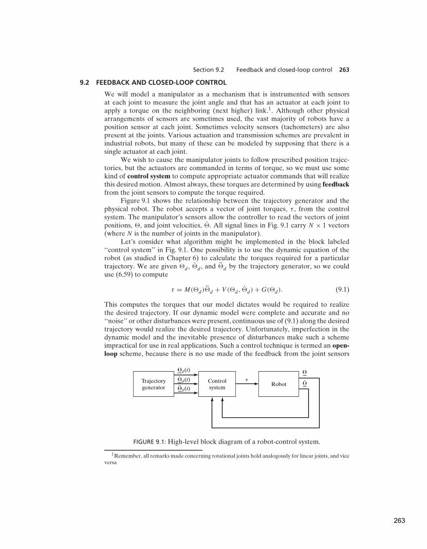
Section 9.2 Feedback and closed-loop control 263
9.2 FEEDBACK AND CLOSED-LOOP CONTROL
We will model a manipulator as a mechanism that is instrumented with sensorsat each joint to measure the joint angle and that has an actuator at each joint toapply a torque on the neighboring (next higher) link.1. Although other physicalarrangements of sensors are sometimes used, the vast majority of robots have aposition sensor at each joint. Sometimes velocity sensors (tachometers) are alsopresent at the joints. Various actuation and transmission schemes are prevalent inindustrial robots, but many of these can be modeled by supposing that there is asingle actuator at each joint.
We wish to cause the manipulator joints to follow prescribed position trajec-tories, but the actuators are commanded in terms of torque, so we must use somekind of control system to compute appropriate actuator commands that will realizethis desired motion. Almost always, these torques are determined by using feedbackfrom the joint sensors to compute the torque required.
Figure 9.1 shows the relationship between the trajectory generator and thephysical robot. The robot accepts a vector of joint torques, τ , from the controlsystem. The manipulator’s sensors allow the controller to read the vectors of jointpositions, �, and joint velocities, �. All signal lines in Fig. 9.1 carry N × 1 vectors(where N is the number of joints in the manipulator).
Let’s consider what algorithm might be implemented in the block labeled‘‘control system’’ in Fig. 9.1. One possibility is to use the dynamic equation of therobot (as studied in Chapter 6) to calculate the torques required for a particulartrajectory. We are given �d , �d , and �d by the trajectory generator, so we coulduse (6.59) to compute
τ = M(�d)�d + V (�d , �d) + G(�d). (9.1)
This computes the torques that our model dictates would be required to realizethe desired trajectory. If our dynamic model were complete and accurate and no‘‘noise’’ or other disturbances were present, continuous use of (9.1) along the desiredtrajectory would realize the desired trajectory. Unfortunately, imperfection in thedynamic model and the inevitable presence of disturbances make such a schemeimpractical for use in real applications. Such a control technique is termed an open-loop scheme, because there is no use made of the feedback from the joint sensors
Trajectorygenerator
Controlsystem
Robot
�d(t)
�d(t).
�d(t).. �
.
�
t
FIGURE 9.1: High-level block diagram of a robot-control system.
1Remember, all remarks made concerning rotational joints hold analogously for linear joints, and viceversa
263
264 Chapter 9 Linear control of manipulators
(i.e., (9.1) is a function only of the desired trajectory, �d , and its derivatives, and not
a function of �, the actual trajectory).Generally, the only way to build a high-performance control system is to make
use of feedback from joint sensors, as indicated in Fig. 9.1. Typically, this feedbackis used to compute any servo error by finding the difference between the desiredand the actual position and that between the desired and the actual velocity:
E = �d − �,
E = �d − �. (9.2)
The control system can then compute how much torque to require of the actuatorsas some function of the servo error. Obviously, the basic idea is to compute actuatortorques that would tend to reduce servo errors. A control system that makes use offeedback is called a closed-loop system. The ‘‘loop’’ closed by such a control systemaround the manipulator is apparent in Fig. 9.1.
The central problem in designing a control system is to ensure that the resultingclosed-loop system meets certain performance specifications. The most basic suchcriterion is that the system remain stable. For our purposes, we will define a systemto be stable if the errors remain ‘‘small’’ when executing various desired trajectorieseven in the presence of some ‘‘moderate’’ disturbances. It should be noted that animproperly designed control system can sometimes result in unstable performance,in which servo errors are enlarged instead of reduced. Hence, the first task of acontrol engineer is to prove that his or her design yields a stable system; the secondis to prove that the closed-loop performance of the system is satisfactory. In practice,such ‘‘proofs’’ range from mathematical proofs based on certain assumptions andmodels to more empirical results, such as those obtained through simulation orexperimentation.
Figure 9.1, in which all signals lines representN×1 vectors, summarizes the factthat the manipulator-control problem is a multi-input, multi-output (MIMO) controlproblem. In this chapter, we take a simple approach to constructing a control systemby treating each joint as a separate system to be controlled. Hence, for an N -jointedmanipulator, we will design N independent single-input, single-output (SISO)control systems. This is the design approach presently adopted by most industrial-robot suppliers. This independent joint control approach is an approximate methodin that the equations of motion (developed in Chapter 6) are not independent, butrather are highly coupled. Later, this chapter will present justification for the linearapproach, at least for the case of highly geared manipulators.
9.3 SECOND-ORDER LINEAR SYSTEMS
Before considering the manipulator control problem, let’s step back and start byconsidering a simple mechanical system. Figure 9.2 shows a block of mass m attachedto a spring of stiffness k and subject to friction of coefficient b. Figure 9.2 also indicatesthe zero position and positive sense of x, the block’s position. Assuming a frictionalforce proportional to the block’s velocity, a free-body diagram of the forces actingon the block leads directly to the equation of motion,
mx + bx + kx = 0. (9.3)
264
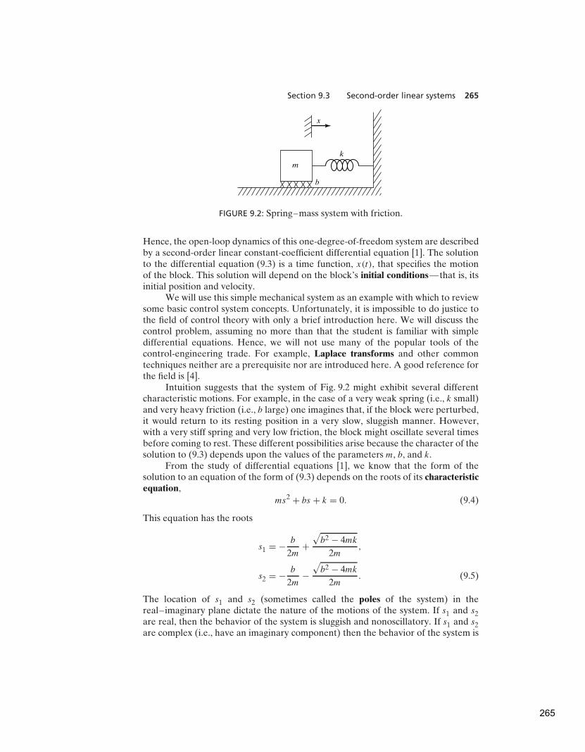
Section 9.3 Second-order linear systems 265
x
m
b
k
FIGURE 9.2: Spring–mass system with friction.
Hence, the open-loop dynamics of this one-degree-of-freedom system are describedby a second-order linear constant-coefficient differential equation [1]. The solutionto the differential equation (9.3) is a time function, x(t), that specifies the motionof the block. This solution will depend on the block’s initial conditions—that is, itsinitial position and velocity.
We will use this simple mechanical system as an example with which to reviewsome basic control system concepts. Unfortunately, it is impossible to do justice tothe field of control theory with only a brief introduction here. We will discuss thecontrol problem, assuming no more than that the student is familiar with simpledifferential equations. Hence, we will not use many of the popular tools of thecontrol-engineering trade. For example, Laplace transforms and other commontechniques neither are a prerequisite nor are introduced here. A good reference forthe field is [4].
Intuition suggests that the system of Fig. 9.2 might exhibit several differentcharacteristic motions. For example, in the case of a very weak spring (i.e., k small)and very heavy friction (i.e., b large) one imagines that, if the block were perturbed,it would return to its resting position in a very slow, sluggish manner. However,with a very stiff spring and very low friction, the block might oscillate several timesbefore coming to rest. These different possibilities arise because the character of thesolution to (9.3) depends upon the values of the parameters m, b, and k.
From the study of differential equations [1], we know that the form of thesolution to an equation of the form of (9.3) depends on the roots of its characteristicequation,
ms2 + bs + k = 0. (9.4)
This equation has the roots
s1 = −b
2m+
√
b2 − 4mk
2m,
s2 = −b
2m−
√
b2 − 4mk
2m. (9.5)
The location of s1 and s2 (sometimes called the poles of the system) in thereal–imaginary plane dictate the nature of the motions of the system. If s1 and s2are real, then the behavior of the system is sluggish and nonoscillatory. If s1 and s2are complex (i.e., have an imaginary component) then the behavior of the system is
265
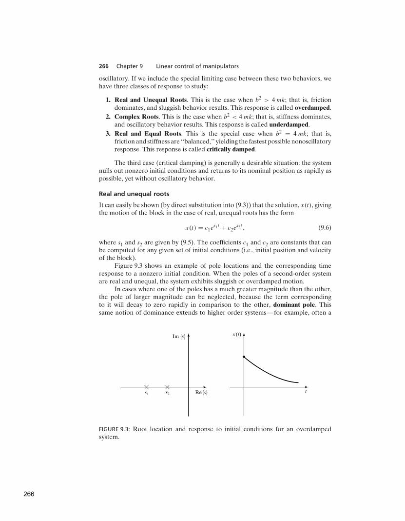
266 Chapter 9 Linear control of manipulators
oscillatory. If we include the special limiting case between these two behaviors, wehave three classes of response to study:
1. Real and Unequal Roots. This is the case when b2 > 4 mk; that is, frictiondominates, and sluggish behavior results. This response is called overdamped.
2. Complex Roots. This is the case when b2 < 4 mk; that is, stiffness dominates,and oscillatory behavior results. This response is called underdamped.
3. Real and Equal Roots. This is the special case when b2 = 4 mk; that is,friction and stiffness are ‘‘balanced,’’ yielding the fastest possible nonoscillatoryresponse. This response is called critically damped.
The third case (critical damping) is generally a desirable situation: the systemnulls out nonzero initial conditions and returns to its nominal position as rapidly aspossible, yet without oscillatory behavior.
Real and unequal roots
It can easily be shown (by direct substitution into (9.3)) that the solution, x(t), givingthe motion of the block in the case of real, unequal roots has the form
x(t) = c1es1t + c2e
s2t , (9.6)
where s1 and s2 are given by (9.5). The coefficients c1 and c2 are constants that canbe computed for any given set of initial conditions (i.e., initial position and velocityof the block).
Figure 9.3 shows an example of pole locations and the corresponding timeresponse to a nonzero initial condition. When the poles of a second-order systemare real and unequal, the system exhibits sluggish or overdamped motion.
In cases where one of the poles has a much greater magnitude than the other,the pole of larger magnitude can be neglected, because the term correspondingto it will decay to zero rapidly in comparison to the other, dominant pole. Thissame notion of dominance extends to higher order systems—for example, often a
Im {s}
s1 s2 Re{s}
x(t)
t
FIGURE 9.3: Root location and response to initial conditions for an overdampedsystem.
266
Section 9.3 Second-order linear systems 267
third-order system can be studied as a second-order system by considering only twodominant poles.
EXAMPLE 9.1
Determine the motion of the system in Fig. 9.2 if parameter values are m = 1, b = 5,and k = 6 and the block (initially at rest) is released from the position x = −1.
The characteristic equation is
s2 + 5s + 6 = 0, (9.7)
which has the roots s1 = −2 and s2 = −3. Hence, the response has the form
x(t) = c1e−2t + c2e
−3t . (9.8)
We now use the given initial conditions, x(0) = −1 and x(0) = 0, to compute c1 andc2. To satisfy these conditions at t = 0, we must have
c1 + c2 = −1
and−2c1 − 3c2 = 0, (9.9)
which are satisfied by c1 = −3 and c2 = 2. So, the motion of the system for t ≥ 0 isgiven by
x(t) = −3e−2t + 2e−3t . (9.10)
Complex roots
For the case where the characteristic equation has complex roots of the form
s1 = λ + µi,
s2 = λ − µi, (9.11)
it is still the case that the solution has the form
x(t) = c1es1t + c2e
s2t . (9.12)
However, equation (9.12) is difficult to use directly, because it involves imaginarynumbers explicitly. It can be shown (see Exercise 9.1) that Euler’s formula,
eix = cos x + i sin x, (9.13)
allows the solution (9.12) to be manipulated into the form
x(t) = c1eλt cos(µt) + c2e
λt sin(µt). (9.14)
As before, the coefficients c1 and c2 are constants that can be computed for anygiven set of initial conditions (i.e., initial position and velocity of the block). If wewrite the constants c1 and c2 in the form
c1 = r cos δ,
c2 = r sin δ, (9.15)
267
268 Chapter 9 Linear control of manipulators
then (9.14) can be written in the form
x(t) = reλt cos(µt − δ), (9.16)
where
r =√
c21
+ c22,
δ = Atan2(c2, c1). (9.17)
In this form, it is easier to see that the resulting motion is an oscillation whoseamplitude is exponentially decreasing toward zero.
Another common way of describing oscillatory second-order systems is interms of damping ratio and natural frequency. These terms are defined by theparameterization of the characteristic equation given by
s2 + 2ζωns + ω2n
= 0, (9.18)
where ζ is the damping ratio (a dimensionless number between 0 and 1) andωn is the natural frequency.2 Relationships between the pole locations and theseparameters are
λ = −ζωn
and
µ = ωn
√
1 − ζ 2. (9.19)
In this terminology, µ, the imaginary part of the poles, is sometimes called thedamped natural frequency. For a damped spring–mass system such as the one inFig. 9.2, the damping ratio and natural frequency are, respectively,
ζ =b
2√km
,
ωn =√
k/m. (9.20)
When no damping is present (b = 0 in our example), the damping ratio becomeszero; for critical damping (b2 = 4km), the damping ratio is 1.
Figure 9.4 shows an example of pole locations and the corresponding timeresponse to a nonzero initial condition. When the poles of a second-order systemare complex, the system exhibits oscillatory or underdamped motion.
EXAMPLE 9.2
Find the motion of the system in Fig. 9.2 if parameter values are m = 1, b = 1, andk = 1 and the block (initially at rest) is released from the position x = −1.
The characteristic equation is
s2 + s + 1 = 0, (9.21)
2The terms damping ratio and natural frequency can also be applied to overdamped systems, in whichcase ζ > 1.0.
268

Section 9.3 Second-order linear systems 269
Im {s}
s1
s2
Re{s}
x(t)
t
FIGURE 9.4: Root location and response to initial conditions for an underdampedsystem.
which has the roots si = − 12 ±
√3
2 i. Hence, the response has the form
x(t) = e− t2
(
c1 cos
√3
2t + c2 sin
√3
2t
)
. (9.22)
We now use the given initial conditions, x(0) = −1 and x(0) = 0, to computec1 and c2. To satisfy these conditions at t = 0, we must have
c1 = −1
and
−1
2c1 −
√3
2c2 = 0, (9.23)
which are satisfied by c1 = −1 and c2 =√
33 . So, the motion of the system for t ≥ 0
is given by
x(t) = e− t2
(
− cos
√3
2t −
√3
3sin
√3
2t
)
. (9.24)
This result can also be put in the form of (9.16), as
x(t) =2√
3
3e− t
2 cos
(√3
2t + 120◦
)
. (9.25)
Real and equal roots
By substitution into (9.3), it can be shown that, in the case of real and equal roots(i.e., repeated roots), the solution has the form
x(t) = c1es1t + c2te
s2t , (9.26)
269
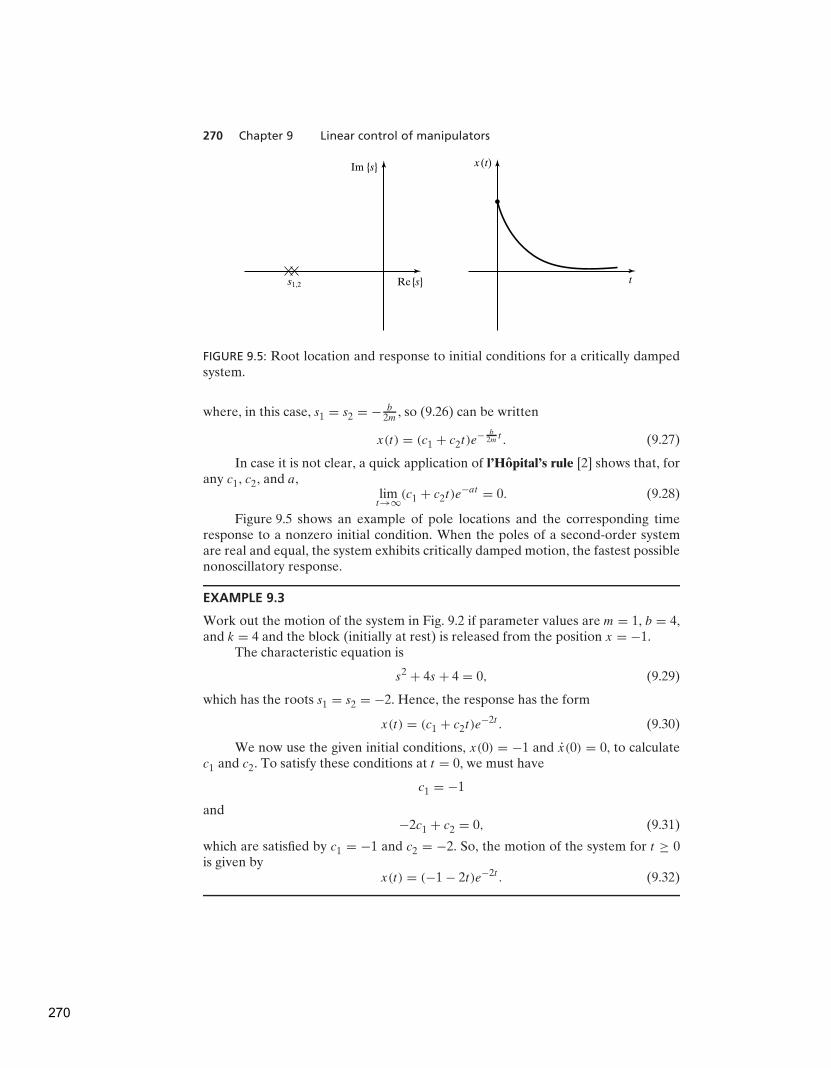
270 Chapter 9 Linear control of manipulators
Im {s}
s1,2 Re{s}
x(t)
t
FIGURE 9.5: Root location and response to initial conditions for a critically dampedsystem.
where, in this case, s1 = s2 = − b2m , so (9.26) can be written
x(t) = (c1 + c2t)e− b
2m t . (9.27)
In case it is not clear, a quick application of l’Hopital’s rule [2] shows that, forany c1, c2, and a,
limt→∞
(c1 + c2t)e−at = 0. (9.28)
Figure 9.5 shows an example of pole locations and the corresponding timeresponse to a nonzero initial condition. When the poles of a second-order systemare real and equal, the system exhibits critically damped motion, the fastest possiblenonoscillatory response.
EXAMPLE 9.3
Work out the motion of the system in Fig. 9.2 if parameter values are m = 1, b = 4,and k = 4 and the block (initially at rest) is released from the position x = −1.
The characteristic equation is
s2 + 4s + 4 = 0, (9.29)
which has the roots s1 = s2 = −2. Hence, the response has the form
x(t) = (c1 + c2t)e−2t . (9.30)
We now use the given initial conditions, x(0) = −1 and x(0) = 0, to calculatec1 and c2. To satisfy these conditions at t = 0, we must have
c1 = −1
and−2c1 + c2 = 0, (9.31)
which are satisfied by c1 = −1 and c2 = −2. So, the motion of the system for t ≥ 0is given by
x(t) = (−1 − 2t)e−2t . (9.32)
270
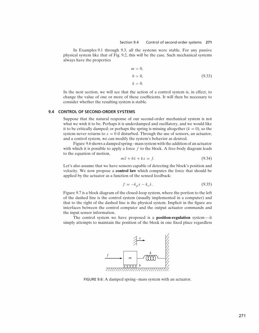
Section 9.4 Control of second-order systems 271
In Examples 9.1 through 9.3, all the systems were stable. For any passivephysical system like that of Fig. 9.2, this will be the case. Such mechanical systemsalways have the properties
m > 0,
b > 0, (9.33)
k > 0.
In the next section, we will see that the action of a control system is, in effect, tochange the value of one or more of these coefficients. It will then be necessary toconsider whether the resulting system is stable.
9.4 CONTROL OF SECOND-ORDER SYSTEMS
Suppose that the natural response of our second-order mechanical system is notwhat we wish it to be. Perhaps it is underdamped and oscillatory, and we would likeit to be critically damped; or perhaps the spring is missing altogether (k = 0), so thesystem never returns to x = 0 if disturbed. Through the use of sensors, an actuator,and a control system, we can modify the system’s behavior as desired.
Figure 9.6 shows a damped spring–mass system with the addition of an actuatorwith which it is possible to apply a force f to the block. A free-body diagram leadsto the equation of motion,
mx + bx + kx = f. (9.34)
Let’s also assume that we have sensors capable of detecting the block’s position andvelocity. We now propose a control law which computes the force that should beapplied by the actuator as a function of the sensed feedback:
f = −kpx − kv x. (9.35)
Figure 9.7 is a block diagram of the closed-loop system, where the portion to the leftof the dashed line is the control system (usually implemented in a computer) andthat to the right of the dashed line is the physical system. Implicit in the figure areinterfaces between the control computer and the output actuator commands andthe input sensor information.
The control system we have proposed is a position-regulation system—itsimply attempts to maintain the position of the block in one fixed place regardless
x
m
b
kf
FIGURE 9.6: A damped spring–mass system with an actuator.
271
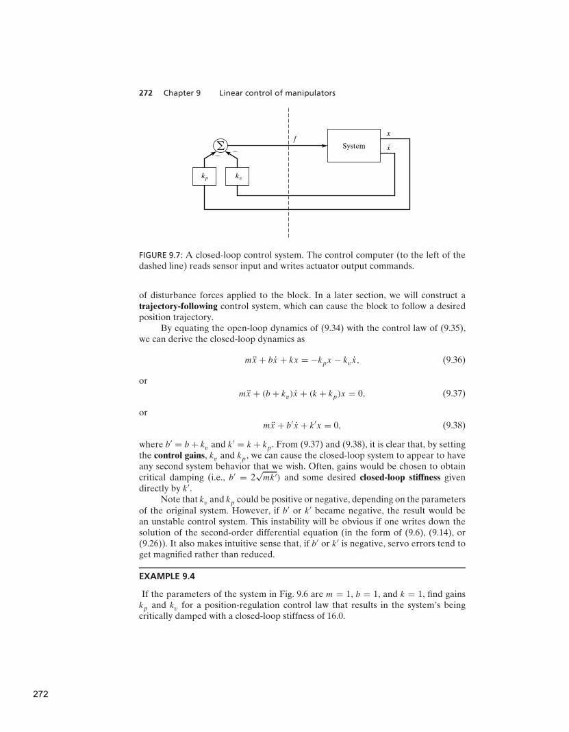
272 Chapter 9 Linear control of manipulators
��
kp kv
fx
x.Systema
FIGURE 9.7: A closed-loop control system. The control computer (to the left of thedashed line) reads sensor input and writes actuator output commands.
of disturbance forces applied to the block. In a later section, we will construct atrajectory-following control system, which can cause the block to follow a desiredposition trajectory.
By equating the open-loop dynamics of (9.34) with the control law of (9.35),we can derive the closed-loop dynamics as
mx + bx + kx = −kpx − kv x, (9.36)
or
mx + (b + kv)x + (k + kp)x = 0, (9.37)
or
mx + b′x + k′x = 0, (9.38)
where b′ = b + kv and k′ = k + kp. From (9.37) and (9.38), it is clear that, by settingthe control gains, kv and kp, we can cause the closed-loop system to appear to haveany second system behavior that we wish. Often, gains would be chosen to obtaincritical damping (i.e., b′ = 2
√mk′) and some desired closed-loop stiffness given
directly by k′.Note that kv and kp could be positive or negative, depending on the parameters
of the original system. However, if b′ or k′ became negative, the result would bean unstable control system. This instability will be obvious if one writes down thesolution of the second-order differential equation (in the form of (9.6), (9.14), or(9.26)). It also makes intuitive sense that, if b′ or k′ is negative, servo errors tend toget magnified rather than reduced.
EXAMPLE 9.4
If the parameters of the system in Fig. 9.6 are m = 1, b = 1, and k = 1, find gainskp and kv for a position-regulation control law that results in the system’s beingcritically damped with a closed-loop stiffness of 16.0.
272

Section 9.5 Control-law partitioning 273
If we wish k′ to be 16.0, then, for critical damping, we require that b′ =2√mk′ = 8.0. Now, k = 1 and b = 1, so we need
kp = 15.0,
kv = 7.0. (9.39)
9.5 CONTROL-LAW PARTITIONING
In preparation for designing control laws for more complicated systems, let usconsider a slightly different controller structure for the sample problem of Fig. 9.6.In this method, we will partition the controller into a model-based portion and aservo portion. The result is that the system’s parameters (i.e.,m, b, and k, in this case)appear only in the model-based portion and that the servo portion is independentof these parameters. At the moment, this distinction might not seem important,but it will become more obviously important as we consider nonlinear systemsin Chapter 10. We will adopt this control-law partitioning approach throughoutthe book.
The open-loop equation of motion for the system is
mx + bx + kx = f. (9.40)
We wish to decompose the controller for this system into two parts. In this case, themodel-based portion of the control law will make use of supposed knowledge of m,b, and k. This portion of the control law is set up such that it reduces the system so
that it appears to be a unit mass. This will become clear when we do Example 9.5.The second part of the control law makes use of feedback to modify the behavior ofthe system. The model-based portion of the control law has the effect of making thesystem appear as a unit mass, so the design of the servo portion is very simple—gainsare chosen to control a system composed of a single unit mass (i.e., no friction, nostiffness).
The model-based portion of the control appears in a control law of the form
f = αf ′ + β, (9.41)
where α and β are functions or constants and are chosen so that, if f ′ is taken as thenew input to the system, the system appears to be a unit mass. With this structure ofthe control law, the system equation (the result of combining (9.40) and (9.41)) is
mx + bx + kx = αf ′ + β. (9.42)
Clearly, in order to make the system appear as a unit mass from the f ′ input, forthis particular system we should choose α and β as follows:
α = m,
β = bx + kx. (9.43)
Making these assignments and plugging them into (9.42), we have the systemequation
x = f ′. (9.44)
273
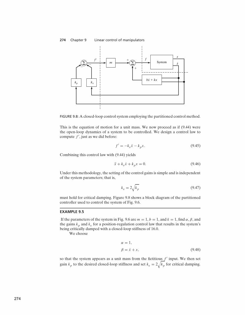
274 Chapter 9 Linear control of manipulators
��
kp kv
fx
x.System
f �m
�
�
bx � kx.
a a
FIGURE 9.8: A closed-loop control system employing the partitioned control method.
This is the equation of motion for a unit mass. We now proceed as if (9.44) werethe open-loop dynamics of a system to be controlled. We design a control law tocompute f ′, just as we did before:
f ′ = −kv x − kpx. (9.45)
Combining this control law with (9.44) yields
x + kv x + kpx = 0. (9.46)
Under this methodology, the setting of the control gains is simple and is independentof the system parameters; that is,
kv = 2√
kp (9.47)
must hold for critical damping. Figure 9.8 shows a block diagram of the partitionedcontroller used to control the system of Fig. 9.6.
EXAMPLE 9.5
If the parameters of the system in Fig. 9.6 are m = 1, b = 1, and k = 1, find α, β, andthe gains kp and kv for a position-regulation control law that results in the system’sbeing critically damped with a closed-loop stiffness of 16.0.
We choose
α = 1,
β = x + x, (9.48)
so that the system appears as a unit mass from the fictitious f ′ input. We then set
gain kp to the desired closed-loop stiffness and set kv = 2√
kp for critical damping.
274

Section 9.6 Trajectory-following control 275
This gives
kp = 16.0,
kv = 8.0. (9.49)
9.6 TRAJECTORY-FOLLOWING CONTROL
Rather than just maintaining the block at a desired location, let us enhance ourcontroller so that the block can be made to follow a trajectory. The trajectory isgiven by a function of time, xd(t), that specifies the desired position of the block.We assume that the trajectory is smooth (i.e., the first two derivatives exist) and thatour trajectory generator provides xd , xd , and xd at all times t . We define the servoerror between the desired and actual trajectory as e = xd − x. A servo-control lawthat will cause trajectory following is
f ′ = xd + kv e + kpe. (9.50)
We see that (9.50) is a good choice if we combine it with the equation of motion ofa unit mass (9.44), which leads to
x = xd + kv e + kpe, (9.51)
ore + kv e + kpe = 0. (9.52)
This is a second-order differential equation for which we can choose the coefficients,so we can design any response we wish. (Often, critical damping is the choice made.)Such an equation is sometimes said to be written in error space, because it describesthe evolution of errors relative to the desired trajectory. Figure 9.9 shows a blockdiagram of our trajectory-following controller.
If our model is perfect (i.e., our knowledge of m, b, and k), and if there isno noise and no initial error, the block will follow the desired trajectory exactly. Ifthere is an initial error, it will be suppressed according to (9.52), and thereafter thesystem will follow the trajectory exactly.
�
�
�
�
�
�
�
kp kv
fx
x.System
f �m
�
�
bx � kx.
xd
.
xd
xd
..
e.
e
aa
a
a
FIGURE 9.9: A trajectory-following controller for the system in Fig. 9.6.
275

276 Chapter 9 Linear control of manipulators
9.7 DISTURBANCE REJECTION
One of the purposes of a control system is to provide disturbance rejection, thatis, to maintain good performance (i.e., minimize errors) even in the presence ofsome external disturbances or noise. In Fig. 9.10, we show the trajectory-followingcontroller with an additional input: a disturbance force fdist. An analysis of ourclosed-loop system leads to the error equation
e + kv e + kpe = fdist. (9.53)
Equation (9.53) is that of a differential equation driven by a forcing function.If it is known that fdist is bounded—that is, that a constant a exists such that
maxt
fdist(t) < a, (9.54)
then the solution of the differential equation, e(t), is also bounded. This result is dueto a property of stable linear systems known as bounded-input, bounded-output orBIBO stability [3, 4]. This very basic result ensures that, for a large class of possibledisturbances, we can at least be assured that the system remains stable.
Steady-state error
Let’s consider the simplest kind of disturbance—namely, that fdist is a constant. Inthis case, we can perform a steady-state analysis by analyzing the system at rest (i.e.,the derivatives of all system variables are zero). Setting derivatives to zero in (9.53)yields the steady-state equation
kpe = fdist, (9.55)
ore = fdist/kp. (9.56)
The value of e given by (9.56) represents a steady-state error. Thus, it is clear thatthe higher the position gain kp, the smaller will be the steady-state error.
�
�
�
�
kp kv
fSystem
f �m
�
�
bx � kx.
xd
.
xd
xd
..
e.
e
fdist
a
a
a
a
FIGURE 9.10: A trajectory-following control system with a disturbance acting.
276

Section 9.8 Continuous vs. discrete time control 277
Addition of an integral term
In order to eliminate steady-state error, a modified control law is sometimes used.The modification involves the addition of an integral term to the control law. Thecontrol law becomes
f ′ = xd + kv e + kpe + ki
∫
edt, (9.57)
which results in the error equation
e + kv e + kpe + ki
∫
edt = fdist. (9.58)
The term is added so that the system will have no steady-state error in the presenceof constant disturbances. If e(t) = 0 for t < 0, we can write (9.58) for t > 0 as
e + kv e + kp e + kie = fdist, (9.59)
which, in the steady state (for a constant disturbance), becomes
kie = 0, (9.60)
so
e = 0. (9.61)
With this control law, the system becomes a third-order system, and one cansolve the corresponding third-order differential equation to work out the responseof the system to initial conditions. Often, ki is kept quite small so that the third-ordersystem is ‘‘close’’ to the second-order system without this term (i.e., a dominant-pole analysis can be performed). The form of control law (9.57) is called a PIDcontrol law, or ‘‘proportional, integral, derivative’’ control law [4]. For simplicity,the displayed equations generally do not show an integral term in the control lawsthat we develop in this book.
9.8 CONTINUOUS VS. DISCRETE TIME CONTROL
In the control systems we have discussed, we implicitly assumed that the controlcomputer performs the computation of the control law in zero time (i.e., infinitelyfast), so that the value of the actuator force f is a continuous function of time. Ofcourse, in reality, the computation requires some time, and the resulting commandedforce is therefore a discrete ‘‘staircase’’ function. We shall employ this approximationof a very fast control computer throughout the book. This approximation is goodif the rate at which new values of f are computed is much faster than the naturalfrequency of the system being controlled. In the field of discrete time control ordigital control, one does not make this approximation but rather takes the servorate of the control system into account when analyzing the system [3].
We will generally assume that the computations can be performed quicklyenough that our continuous time assumption is valid. This raises a question: Howquick is quick enough? There are several points that need to be considered inchoosing a sufficiently fast servo (or sample) rate:
277

278 Chapter 9 Linear control of manipulators
Tracking reference inputs: The frequency content of the desired or reference inputplaces an absolute lower bound on the sample rate. The sample rate must beat least twice the bandwidth of reference inputs. This is usually not the limitingfactor.
Disturbance rejection: In disturbance rejection, an upper bound on performanceis given by a continuous-time system. If the sample period is longer than thecorrelation time of the disturbance effects (assuming a statistical model forrandom disturbances), then these disturbances will not be suppressed. Perhapsa good rule of thumb is that the sample period should be 10 times shorter thanthe correlation time of the noise [3].
Antialiasing: Any time an analog sensor is used in a digital control scheme, therewill be a problem with aliasing unless the sensor’s output is strictly bandlimited. In most cases, sensors do not have a band limited output, and sosample rate should be chosen such that the amount of energy that appears inthe aliased signal is small.
Structural resonances: We have not included bending modes in our characterizationof a manipulator’s dynamics. All real mechanisms have finite stiffness and sowill be subject to various kinds of vibrations. If it is important to suppress thesevibrations (and it often is), we must choose a sample rate at least twice thenatural frequency of these resonances. We will return to the topic of resonancelater in this chapter.
9.9 MODELING AND CONTROL OF A SINGLE JOINT
In this section, we will develop a simplified model of a single rotary joint of amanipulator. A few assumptions will be made that will allow us to model theresulting system as a second-order linear system. For a more complete model of anactuated joint, see [5].
A common actuator found in many industrial robots is the direct current (DC)torque motor (as in Fig. 8.18). The nonturning part of the motor (the stator) consistsof a housing, bearings, and either permanent magnets or electromagnets. Thesestator magnets establish a magnetic field across the turning part of the motor (therotor). The rotor consists of a shaft and windings through which current moves topower the motor. The current is conducted to the windings via brushes, which makecontact with the commutator. The commutator is wired to the various windings (alsocalled the armature) in such a way that torque is always produced in the desireddirection. The underlying physical phenomenon [6] that causes a motor to generatea torque when current passes through the windings can be expressed as
F = qV × B, (9.62)
where charge q, moving with velocity V through a magnetic field B, experiences aforce F . The charges are those of electrons moving through the windings, and themagnetic field is that set up by the stator magnets. Generally, the torque-producingability of a motor is stated by means of a single motor torque constant, which relatesarmature current to the output torque as
τm = kmia . (9.63)
278
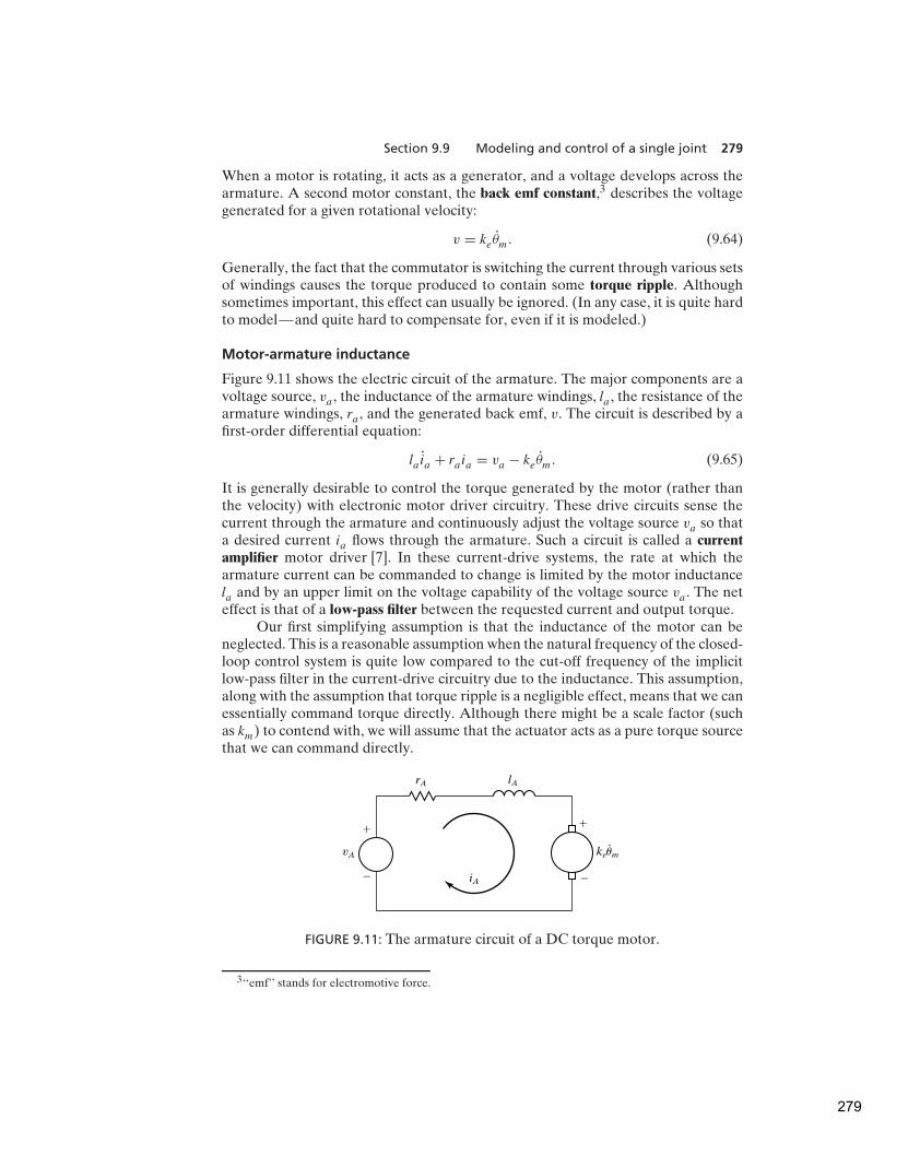
Section 9.9 Modeling and control of a single joint 279
When a motor is rotating, it acts as a generator, and a voltage develops across thearmature. A second motor constant, the back emf constant,3 describes the voltagegenerated for a given rotational velocity:
v = ke θm. (9.64)
Generally, the fact that the commutator is switching the current through various setsof windings causes the torque produced to contain some torque ripple. Althoughsometimes important, this effect can usually be ignored. (In any case, it is quite hardto model—and quite hard to compensate for, even if it is modeled.)
Motor-armature inductance
Figure 9.11 shows the electric circuit of the armature. The major components are avoltage source, va , the inductance of the armature windings, la , the resistance of thearmature windings, ra , and the generated back emf, v. The circuit is described by afirst-order differential equation:
la ia + raia = va − ke θm. (9.65)
It is generally desirable to control the torque generated by the motor (rather thanthe velocity) with electronic motor driver circuitry. These drive circuits sense thecurrent through the armature and continuously adjust the voltage source va so thata desired current ia flows through the armature. Such a circuit is called a currentamplifier motor driver [7]. In these current-drive systems, the rate at which thearmature current can be commanded to change is limited by the motor inductancela and by an upper limit on the voltage capability of the voltage source va . The neteffect is that of a low-pass filter between the requested current and output torque.
Our first simplifying assumption is that the inductance of the motor can beneglected. This is a reasonable assumption when the natural frequency of the closed-loop control system is quite low compared to the cut-off frequency of the implicitlow-pass filter in the current-drive circuitry due to the inductance. This assumption,along with the assumption that torque ripple is a negligible effect, means that we canessentially command torque directly. Although there might be a scale factor (suchas km) to contend with, we will assume that the actuator acts as a pure torque sourcethat we can command directly.
�
�
vA
rA lA
iA
�
�
keum
.
FIGURE 9.11: The armature circuit of a DC torque motor.
3‘‘emf’’ stands for electromotive force.
279
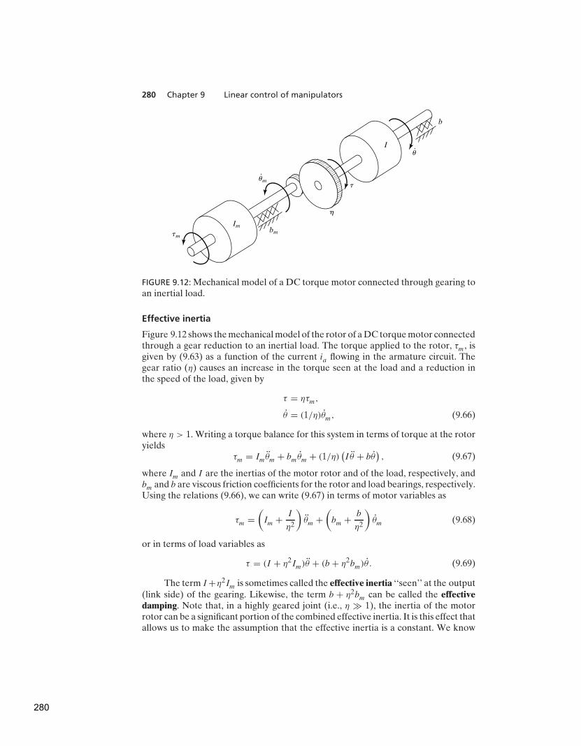
280 Chapter 9 Linear control of manipulators
tm
Imbm
h
t
Iu
b
um
.
.
FIGURE 9.12: Mechanical model of a DC torque motor connected through gearing toan inertial load.
Effective inertia
Figure 9.12 shows the mechanical model of the rotor of a DC torque motor connectedthrough a gear reduction to an inertial load. The torque applied to the rotor, τm, isgiven by (9.63) as a function of the current ia flowing in the armature circuit. Thegear ratio (η) causes an increase in the torque seen at the load and a reduction inthe speed of the load, given by
τ = ητm,
θ = (1/η)θm, (9.66)
where η > 1. Writing a torque balance for this system in terms of torque at the rotoryields
τm = Imθm + bmθm + (1/η)(
I θ + bθ)
, (9.67)
where Im and I are the inertias of the motor rotor and of the load, respectively, andbm and b are viscous friction coefficients for the rotor and load bearings, respectively.Using the relations (9.66), we can write (9.67) in terms of motor variables as
τm =(
Im +I
η2
)
θm +(
bm +b
η2
)
θm (9.68)
or in terms of load variables as
τ = (I + η2Im)θ + (b + η2bm)θ . (9.69)
The term I +η2Im is sometimes called the effective inertia ‘‘seen’’ at the output(link side) of the gearing. Likewise, the term b + η2bm can be called the effectivedamping. Note that, in a highly geared joint (i.e., η ≫ 1), the inertia of the motorrotor can be a significant portion of the combined effective inertia. It is this effect thatallows us to make the assumption that the effective inertia is a constant. We know
280
Section 9.9 Modeling and control of a single joint 281
from Chapter 6 that the inertia, I , of a joint of the mechanism actually varies withconfiguration and load. However, in highly geared robots, the variations representa smaller percentage than they would in a direct-drive manipulator (i.e., η = 1). Toensure that the motion of the robot link is never underdamped, the value used for Ishould be the maximum of the range of values that I takes on; we’ll call this valueImax. This choice results in a system that is critically damped or overdamped in allsituations. In Chapter 10, we will deal with varying inertia directly and will not haveto make this assumption.
EXAMPLE 9.6
If the apparent link inertia, I , varies between 2 and 6 Kg-m2, the rotor inertia isIm = 0.01, and the gear ratio is η = 30, what are the minimum and maximum of theeffective inertia?
The minimum effective inertia is
Imin + η2Im = 2.0 + (900)(0.01) = 11.0; (9.70)
the maximum isImax + η2Im = 6.0 + (900)(0.01) = 15.0. (9.71)
Hence, we see that, as a percentage of the total effective inertia, the variation ofinertia is reduced by the gearing.
Unmodeled flexibility
The other major assumption we have made in our model is that the gearing, theshafts, the bearings, and the driven link are not flexible. In reality, all of theseelements have finite stiffness, and their flexibility, if modeled, would increase theorder of the system. The argument for ignoring flexibility effects is that, if the systemis sufficiently stiff, the natural frequencies of these unmodeled resonances are veryhigh and can be neglected compared to the influence of the dominant second-orderpoles that we have modeled.4 The term ‘‘unmodeled’’ refers to the fact that, forpurposes of control-system analysis and design, we neglect these effects and use asimpler dynamic model, such as (9.69).
Because we have chosen not to model structural flexibilities in the system,we must be careful not to excite these resonances. A rule of thumb [8] is that, ifthe lowest structural resonance is ωres, then we must limit our closed-loop naturalfrequency according to
ωn ≤1
2ωres. (9.72)
This provides some guidance on how to choose gains in our controller. We have seenthat increasing gains leads to faster response and lower steady-state error, but wenow see that unmodeled structural resonances limit the magnitude of gains. Typicalindustrial manipulators have structural resonances in the range from 5 Hz to 25 Hz[8]. Recent designs using direct-drive arrangements that do not contain flexibility
4This is basically the same argument we used to neglect the pole due to the motor inductance.Including it would also have raised the order of the overall system.
281
282 Chapter 9 Linear control of manipulators
introduced by reduction and transmission systems have their lowest structuralresonances as high as 70 Hz [9].
EXAMPLE 9.7
Consider the system of Fig. 9.7 with the parameter values m = 1, b = 1, and k = 1.Additionally, it is known that the lowest unmodeled resonance of the system is at8 radians/second. Find α, β, and gains kp and kv for a position-control law so thesystem is critically damped, doesn’t excite unmodeled dynamics, and has as high aclosed-loop stiffness as possible.
We choose
α = 1,
β = x + x, (9.73)
so that the system appears as a unit mass from the fictitious f ′ input. Usingour rule of thumb (9.72), we choose the closed-loop natural frequency to beωn = 4 radians/second. From (9.18) and (9.46), we have kp = ω2
n, so
kp = 16.0,
kv = 8.0. (9.74)
Estimating resonant frequency
The same sources of structural flexibility discussed in Chapter 8 give rise to reso-nances. In each case where a structural flexibility can be identified, an approximateanalysis of the resulting vibration is possible if we can describe the effective massor inertia of the flexible member. This is done by approximating the situation by asimple spring–mass system, which, as given in (9.20), exhibits the natural frequency
ωn =√
k/m, (9.75)
where k is the stiffness of the flexible member and m is the equivalent mass displacedin vibrations.
EXAMPLE 9.8
A shaft (assumed massless) with a stiffness of 400 Nt-m/radian drives a rotationalinertia of 1 Kg-m2. If the shaft stiffness was neglected in the modeling of thedynamics, what is the frequency of this unmodeled resonance?
Using (9.75), we have
ωres =√
400/1 = 20 rad/second = 20/(2π)Hz ∼= 3.2 Hz. (9.76)
For the purposes of a rough estimate of the lowest resonant frequency ofbeams and shafts, [10] suggests using a lumped model of the mass. We already
282
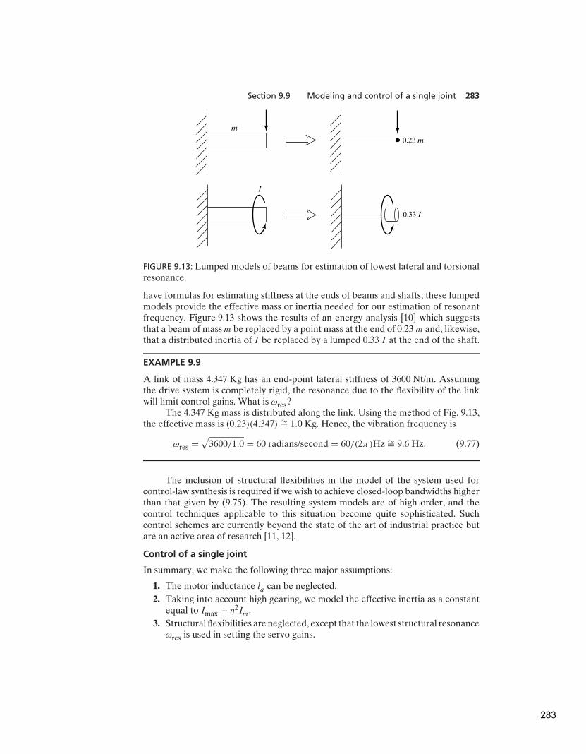
Section 9.9 Modeling and control of a single joint 283
m
I
0.23 m
0.33 I
FIGURE 9.13: Lumped models of beams for estimation of lowest lateral and torsionalresonance.
have formulas for estimating stiffness at the ends of beams and shafts; these lumpedmodels provide the effective mass or inertia needed for our estimation of resonantfrequency. Figure 9.13 shows the results of an energy analysis [10] which suggeststhat a beam of mass m be replaced by a point mass at the end of 0.23 m and, likewise,that a distributed inertia of I be replaced by a lumped 0.33 I at the end of the shaft.
EXAMPLE 9.9
A link of mass 4.347 Kg has an end-point lateral stiffness of 3600 Nt/m. Assumingthe drive system is completely rigid, the resonance due to the flexibility of the linkwill limit control gains. What is ωres?
The 4.347 Kg mass is distributed along the link. Using the method of Fig. 9.13,the effective mass is (0.23)(4.347) ∼= 1.0 Kg. Hence, the vibration frequency is
ωres =√
3600/1.0 = 60 radians/second = 60/(2π)Hz ∼= 9.6 Hz. (9.77)
The inclusion of structural flexibilities in the model of the system used forcontrol-law synthesis is required if we wish to achieve closed-loop bandwidths higherthan that given by (9.75). The resulting system models are of high order, and thecontrol techniques applicable to this situation become quite sophisticated. Suchcontrol schemes are currently beyond the state of the art of industrial practice butare an active area of research [11, 12].
Control of a single joint
In summary, we make the following three major assumptions:
1. The motor inductance la can be neglected.
2. Taking into account high gearing, we model the effective inertia as a constantequal to Imax + η2Im.
3. Structural flexibilities are neglected, except that the lowest structural resonanceωres is used in setting the servo gains.
283

284 Chapter 9 Linear control of manipulators
With these assumptions, a single joint of a manipulator can be controlled withthe partitioned controller given by
α = Imax + η2Im,
β = (b + η2bm)θ , (9.78)
τ ′ = θd + kv e + kpe. (9.79)
The resulting system closed-loop dynamics are
e + kv e + kpe = τdist, (9.80)
where the gains are chosen as
kp = ω2n
=1
4ω2
res,
kv = 2√
kp = ωres. (9.81)
9.10 ARCHITECTURE OF AN INDUSTRIAL-ROBOT CONTROLLER
In this section, we briefly look at the architecture of the control system of theUnimation PUMA 560 industrial robot. As shown in Fig. 9.14, the hardware archi-tecture is that of a two-level hierarchy, with a DEC LSI-11 computer serving asthe top-level ‘‘master’’ control computer passing commands to six Rockwell 6503microprocessors.5 Each of these microprocessors controls an individual joint witha PID control law not unlike that presented in this chapter. Each joint of thePUMA 560 is instrumented with an incremental optical encoder. The encoders areinterfaced to an up/down counter, which the microprocessor can read to obtain thecurrent joint position. There are no tachometers in the PUMA 560; rather, jointpositions are differenced on subsequent servo cycles to obtain an estimate of jointvelocity. In order to command torques to the DC torque motors, the microprocessor
VALlanguage
DECLSI-11
Interface
6503
6503
6503
6503
6503
6503
Joint 1
Joint 2
Joint 3
Joint 4
Joint 5
Joint 6
FIGURE 9.14: Hierarchical computer architecture of the PUMA 560 robot-controlsystem.
5These simple 8-bit computers are already old technology. It is common these days for robotcontrollers to be based on 32-bit microprocessors.
284

Bibliography 285
ud6503 D/A
CurrentAmp.
iAMotor
u(t)
Encoder
u
FIGURE 9.15: Functional blocks of the joint-control system of the PUMA 560.
is interfaced to a digital-to-analog converter (DAC) so that motor currents can becommanded to the current-driver circuits. The current flowing through the motor iscontrolled in analog circuitry by adjusting the voltage across the armature as neededto maintain the desired armature current. A block diagram is shown in Fig. 9.15.
Each 28 milliseconds, the LSI-11 computer sends a new position command(set-point) to the joint microprocessors. The joint microprocessors are running on a0.875 millisecond cycle. In this time, they interpolate the desired position set-point,compute the servo error, compute the PID control law, and command a new valueof torque to the motors.
The LSI-11 computer carries out all the ‘‘high-level’’ operations of the overallcontrol system. First of all, it takes care of interpreting the VAL (Unimation’srobot programming language) program commands one by one. When a motioncommand is interpreted, the LSI-11 must perform any needed inverse kinematiccomputations, plan a desired trajectory, and begin generating trajectory via pointsevery 28 milliseconds for the joint controllers.
The LSI-11 is also interfaced to such standard peripherals as the terminal anda floppy disk drive. In addition, it is interfaced to a teach pendant. A teach pendantis a handheld button box that allows the operator to move the robot around in avariety of modes. For example, the PUMA 560 system allows the user to move therobot incrementally in joint coordinates or in Cartesian coordinates from the teachpendant. In this mode, teach-pendant buttons cause a trajectory to be computed‘‘on the fly’’ and passed down to the joint-control microprocessors.
BIBLIOGRAPHY
[1] W. Boyce and R. DiPrima, Elementary Differential Equations, 3rd edition, John Wileyand Sons, New York, 1977.
[2] E. Purcell, Calculus with Analytic Geometry, Meredith Corporation, New York, 1972.
[3] G. Franklin and J.D. Powell, Digital Control of Dynamic Systems, Addison-Wesley,Reading, MA, 1980.
[4] G. Franklin, J.D. Powell, and A. Emami-Naeini, Feedback Control of Dynamic Sys-
tems, Addison-Wesley, Reading, MA, 1986.
[5] J. Luh, ‘‘Conventional Controller Design for Industrial Robots—a Tutorial,’’ IEEE
Transactions on Systems, Man, and Cybernetics, Vol. SMC-13, No. 3, June 1983.
[6] D. Halliday and R. Resnik, Fundamentals of Physics, Wiley, New York 1970.
285
286 Chapter 9 Linear control of manipulators
[7] Y. Koren and A. Ulsoy, ‘‘Control of DC Servo-Motor Driven Robots,’’ Proceedings
of Robots 6 Conference, SME, Detroit, March 1982.
[8] R.P. Paul, Robot Manipulators, MIT Press, Cambridge, MA, 1981.
[9] H. Asada and K. Youcef-Toumi, Direct-Drive Robots—Theory and Practice, MITPress, Cambridge, MA, 1987.
[10] J. Shigley, Mechanical Engineering Design, 3rd edition, McGraw-Hill, New York, 1977.
[11] W. Book, ‘‘Recursive Lagrangian Dynamics of Flexible Manipulator Arms,’’ The
International Journal of Robotics Research, Vol. 3, No. 3, 1984.
[12] R. Cannon and E. Schmitz, ‘‘Initial Experiments on the End-Point Control of aFlexible One Link Robot,’’ The International Journal of Robotics Research, Vol. 3,No. 3, 1984.
[13] R.J. Nyzen, ‘‘Analysis and Control of an Eight-Degree-of-Freedom Manipulator,’’Ohio University Master’s Thesis, Mechanical Engineering, Dr. Robert L. Williams II,Advisor, August 1999.
[14] R.L. Williams II, ‘‘Local Performance Optimization for a Class of Redundant Eight-
Degree-of-Freedom Manipulators,’’ NASA Technical Paper 3417, NASA LangleyResearch Center, Hampton, VA, March 1994.
EXERCISES
9.1 [20] For a second-order differential equation with complex roots
s1 = λ + µi,
s2 = λ − µi,
show that the general solution
x(t) = c1es1t + c2e
s2t ,
can be writtenx(t) = c1e
λt cos(µt) + c2eλt sin(µt).
9.2 [13] Compute the motion of the system in Fig. 9.2 if parameter values are m = 2,b = 6, and k = 4 and the block (initially at rest) is released from the positionx = 1.
9.3 [13] Compute the motion of the system in Fig. 9.2 if parameter values are m = 1,b = 2, and k = 1 and the block (initially at rest) is released from the positionx = 4.
9.4 [13] Compute the motion of the system in Fig. 9.2 if parameter values are m = 1,b = 4, and k = 5 and the block (initially at rest) is released from the positionx = 2.
9.5 [15] Compute the motion of the system in Fig. 9.2 if parameter values are m = 1,b = 7, and k = 10 and the block is released from the position x = 1 with an initialvelocity of x = 2.
9.6 [15] Use the (1, 1) element of (6.60) to compute the variation (as a percentageof the maximum) of the inertia ‘‘seen’’ by joint 1 of this robot as it changesconfiguration. Use the numerical values
l1 = l2 = 0.5 m,
m1 = 4.0 Kg,
m2 = 2.0 Kg.
286

Programming exercise (Part 9) 287
Consider that the robot is direct drive and that the rotor inertia is negligible.9.7 [17] Repeat Exercise 9.6 for the case of a geared robot (use η = 20) and a rotor
inertia of Im = 0.01 Kg m2.9.8 [18] Consider the system of Fig. 9.6 with the parameter values m = 1, b = 4,
and k = 5. The system is also known to possess an unmodeled resonance atωres = 6.0 radians/second. Determine the gains kv and kp that will critically dampthe system with as high a stiffness as is reasonable.
9.9 [25] In a system like that of Fig. 9.12, the inertial load, I , varies between 4 and5 Kg-m2. The rotor inertia is Im = 0.01 Kg-m2, and the gear ratio is η = 10.The system possesses unmodeled resonances at 8.0, 12.0, and 20.0 radians/second.Design α and β of the partitioned controller and give the values of kp and kv suchthat the system is never underdamped and never excites resonances, but is as stiffas possible.
9.10 [18] A designer of a direct-drive robot suspects that the resonance due to beamflexibility of the link itself will be the cause of the lowest unmodeled resonance. Ifthe link is approximately a square-cross-section beam of dimensions 5×5×50 cmwith a 1-cm wall thickness and a total mass of 5 Kg, estimate ωres.
9.11 [15]A direct-drive robot link is driven through a shaft of stiffness 1000 Nt-m/radian.The link inertia is 1 Kg-m2. Assuming the shaft is massless, what is ωres?
9.12 [18] A shaft of stiffness 500 Nt-m/radian drives the input of a rigid gear pair withη = 8. The output of the gears drives a rigid link of inertia 1 Kg-m2. What is theωres caused by flexibility of the shaft?
9.13 [25] A shaft of stiffness 500 Nt-m/radian drives the input of a rigid gear pair withη = 8. The shaft has an inertia of 0.1 Kg-m2. The output of the gears drives a rigidlink of inertia 1 Kg-m2. What is the ωres caused by flexibility of the shaft?
9.14 [28] In a system like that of Fig. 9.12, the inertial load, I , varies between 4 and5 Kg-m2. The rotor inertia is Im = 0.01 Kg-m2, and the gear ratio is η = 10. Thesystem possesses an unmodeled resonance due to an end-point stiffness of thelink of 2400 Nt-m/radian. Design α and β of the partitioned controller, and givethe values of kp and kv such that the system is never underdamped and neverexcites resonances, but is as stiff as possible.
9.15 [25] A steel shaft of length 30 cm and diameter 0.2 cm drives the input gear of areduction of η = 8. The rigid output gear drives a steel shaft of length 30 cm anddiameter 0.3 cm. What is the range of resonant frequencies observed if the loadinertia varies between 1 and 4 Kg-m2?
PROGRAMMING EXERCISE (PART 9)
We wish to simulate a simple trajectory-following control system for the three-link planararm. This control system will be implemented as an independent-joint PD (proportionalplus derivative) control law. Set the servo gains to achieve closed-loop stiffnesses of175.0, 110.0, and 20.0 for joints 1 through 3 respectively. Try to achieve approximatecritical damping.
Use the simulation routine UPDATE to simulate a discrete-time servo runningat 100 Hz—that is, calculate the control law at 100 Hz, not at the frequency of thenumerical integration process. Test the control scheme on the following tests:
1. Start the arm at � = (60,−110, 20) and command it to stay there until t ime = 3.0,when the set-points should instantly change to � = (60,−50, 20). That is, give astep input of 60 degrees to joint 2. Record the error–time history for each joint.
2. Control the arm to follow the cubic-spline trajectory from Programming ExercisePart 7. Record the error–time history for each joint.
287
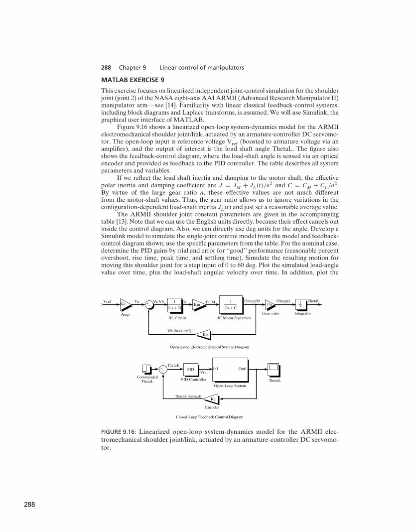
288 Chapter 9 Linear control of manipulators
MATLAB EXERCISE 9
This exercise focuses on linearized independent joint-control simulation for the shoulderjoint (joint 2) of the NASA eight-axis AAI ARMII (Advanced Research Manipulator II)manipulator arm—see [14]. Familiarity with linear classical feedback-control systems,including block diagrams and Laplace transforms, is assumed. We will use Simulink, thegraphical user interface of MATLAB.
Figure 9.16 shows a linearized open-loop system-dynamics model for the ARMIIelectromechanical shoulder joint/link, actuated by an armature-controller DC servomo-tor. The open-loop input is reference voltage Vref (boosted to armature voltage via anamplifier), and the output of interest is the load shaft angle ThetaL. The figure alsoshows the feedback-control diagram, where the load-shaft angle is sensed via an opticalencoder and provided as feedback to the PID controller. The table describes all systemparameters and variables.
If we reflect the load shaft inertia and damping to the motor shaft, the effectivepolar inertia and damping coefficient are J = JM + JL(t)/n
2 and C = CM + CL/n2.
By virtue of the large gear ratio n, these effective values are not much differentfrom the motor-shaft values. Thus, the gear ratio allows us to ignore variations in theconfiguration-dependent load-shaft inertia JL(t) and just set a reasonable average value.
The ARMII shoulder joint constant parameters are given in the accompanyingtable [13]. Note that we can use the English units directly, because their effect cancels outinside the control diagram. Also, we can directly use deg units for the angle. Develop aSimulink model to simulate the single-joint control model from the model and feedback-control diagram shown; use the specific parameters from the table. For the nominal case,determine the PID gains by trial and error for ‘‘good’’ performance (reasonable percentovershoot, rise time, peak time, and settling time). Simulate the resulting motion formoving this shoulder joint for a step input of 0 to 60 deg. Plot the simulated load-anglevalue over time, plus the load-shaft angular velocity over time. In addition, plot the
Vref Va 1Ka
Va-Vb laKm
Ke
TauM OmegaM
JC Motor DynamicsGear ratio Integrator
ThetaLOmegaL1/n
L.s � R
AmpRL Circuit
Vb (back emf)
CommandedThetaL
VrefPID
Kb
Encoder
PID Controller
Open-Loop System
In1 Out1ThetaE
ThetaS (sensed)
ThetaL
��
��
Open-Loop Electromechanical System Diagram
Closed-Loop Feedback Control Diagram
1
J.s � C
1s
FIGURE 9.16: Linearized open-loop system-dynamics model for the ARMII elec-tromechanical shoulder joint/link, actuated by an armature-controller DC servomo-tor.
288

MATLAB Exercise 9 289
TABLE 9.1: ARMII shoulder joint constant parameters.
Va(t) armaturevoltage
τM(t) generatedmotortorque
τL(t) load torque
L = 0.0006H armatureinduc-tance
θM(t) motor shaftangle
θL(t) load shaftangle
R = 1.403 armatureresis-tance
ωM(t) motor shaftvelocity
ωL(t) load shaftvelocity
ia(t) armaturecurrent
JM = 0.00844
lbf -in-s2lumpedmotor polarinertia
JL(t) = 1
lbf -in-s2lumped loadpolar inertia
Vb(t) back emfvoltage
CM = 0.00013lbf -in/deg/s
motor shaftviscousdampingcoefficient
CL = 0.5lbf -in/deg/s
load shaftviscousdampingcoefficient
Ka = 12 amplifiergain
n = 200 gear ratio g = 0in/s2
gravity(ignoregravity atfirst)
Kb = 0.00867V/deg/s
back emfconstant
KM = 4.375lbf -in/A
torque con-stant
Ke = 1 encodertransferfunction
control effort—that is, the armature voltage Va over time. (On the same graph, also givethe back emf Vb.)
Now, try some changes—Simulink is so easy and enjoyable to change:
1) The step input is frustrating for controller design, so try a ramped step inputinstead: Ramp from 0 to 60 deg in 1.5 sec, then hold the 60-deg command for alltime greater than 1.5 sec. Redesign PID gains and restimulate.
2) Investigate whether the inductor L is significant in this system. (The electrical sys-tem rises much faster than the mechanical system—this effect can be representedby time constants.)
3) We don’t have a good estimate for the load inertia and damping (JL and CL). Withyour best PID gains from before, investigate how big these values can grow (scalethe nominal parameters up equally) before they affect the system.
4) Now, include the effect of gravity as a disturbance to the motor torque TM . Assumethat the moving robot mass is 200 lb and the moving length beyond joint 2 is 6.4feet. Test for the nominal ‘‘good’’ PID gains you found; redesign if necessary. Theshoulder load angle θ2 zero configuration is straight up.
289
C H A P T E R 10
Nonlinear controlof manipulators
10.1 INTRODUCTION
10.2 NONLINEAR AND TIME-VARYING SYSTEMS
10.3 MULTI-INPUT, MULTI-OUTPUT CONTROL SYSTEMS
10.4 THE CONTROL PROBLEM FOR MANIPULATORS
10.5 PRACTICAL CONSIDERATIONS
10.6 CURRENT INDUSTRIAL-ROBOT CONTROL SYSTEMS
10.7 LYAPUNOV STABILITY ANALYSIS
10.8 CARTESIAN-BASED CONTROL SYSTEMS
10.9 ADAPTIVE CONTROL
10.1 INTRODUCTION
In the previous chapter, we made several approximations to allow a linear analysis ofthe manipulator-control problem. Most important among these approximations wasthat each joint could be considered independent and that the inertia ‘‘seen’’ by eachjoint actuator was constant. In implementations of linear controllers as introduced inthe previous chapter, this approximation results in nonuniform damping throughoutthe workspace and other undesirable effects. In this chapter, we will introduce amore advanced control technique for which this assumption will not have to bemade.
In Chapter 9, we modeled the manipulator by n independent second-orderdifferential equations and based our controller on that model. In this chapter, wewill base our controller design directly on the n × 1-nonlinear vector differentialequation of motion, derived in Chapter 6 for a general manipulator.
The field of nonlinear control theory is large; we must therefore restrict ourattention to one or two methods that seem well suited to mechanical manipulators.Consequently, the major focus of the chapter will be one particular method,apparently first proposed in [1] and named the computed-torque method in [2, 3].We will also introduce one method of stability analysis of nonlinear systems, knownas Lyapunov’s method [4].
To begin our discussion of nonlinear techniques for controlling a manipulator,we return again to a very simple single-degree-of-freedom mass–spring frictionsystem.
From Chapter 10 of Introduction to Robotics: Mechanics and Control, Third Edition. John J. Craig.
Copyright © 2005 by Pearson Education, Inc. All rights reserved.
290
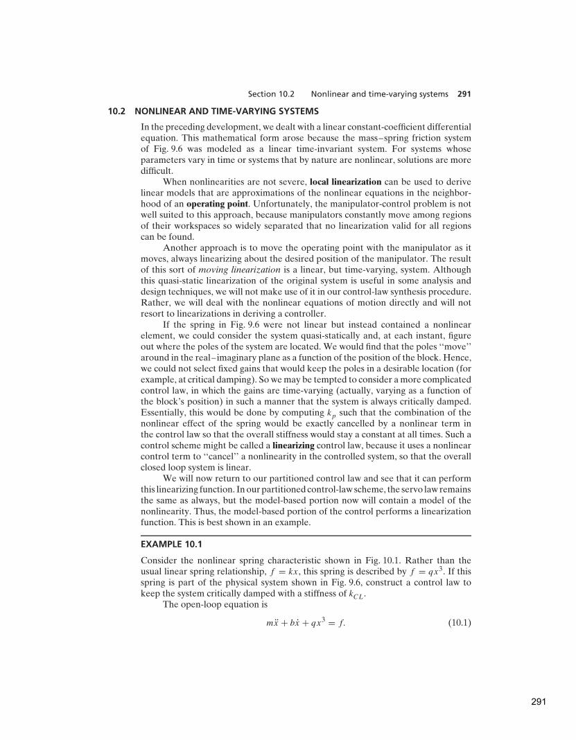
Section 10.2 Nonlinear and time-varying systems 291
10.2 NONLINEAR AND TIME-VARYING SYSTEMS
In the preceding development, we dealt with a linear constant-coefficient differentialequation. This mathematical form arose because the mass–spring friction systemof Fig. 9.6 was modeled as a linear time-invariant system. For systems whoseparameters vary in time or systems that by nature are nonlinear, solutions are moredifficult.
When nonlinearities are not severe, local linearization can be used to derivelinear models that are approximations of the nonlinear equations in the neighbor-hood of an operating point. Unfortunately, the manipulator-control problem is notwell suited to this approach, because manipulators constantly move among regionsof their workspaces so widely separated that no linearization valid for all regionscan be found.
Another approach is to move the operating point with the manipulator as itmoves, always linearizing about the desired position of the manipulator. The resultof this sort of moving linearization is a linear, but time-varying, system. Althoughthis quasi-static linearization of the original system is useful in some analysis anddesign techniques, we will not make use of it in our control-law synthesis procedure.Rather, we will deal with the nonlinear equations of motion directly and will notresort to linearizations in deriving a controller.
If the spring in Fig. 9.6 were not linear but instead contained a nonlinearelement, we could consider the system quasi-statically and, at each instant, figureout where the poles of the system are located. We would find that the poles ‘‘move’’around in the real–imaginary plane as a function of the position of the block. Hence,we could not select fixed gains that would keep the poles in a desirable location (forexample, at critical damping). So we may be tempted to consider a more complicatedcontrol law, in which the gains are time-varying (actually, varying as a function ofthe block’s position) in such a manner that the system is always critically damped.Essentially, this would be done by computing kp such that the combination of thenonlinear effect of the spring would be exactly cancelled by a nonlinear term inthe control law so that the overall stiffness would stay a constant at all times. Such acontrol scheme might be called a linearizing control law, because it uses a nonlinearcontrol term to ‘‘cancel’’ a nonlinearity in the controlled system, so that the overallclosed loop system is linear.
We will now return to our partitioned control law and see that it can performthis linearizing function. In our partitioned control-law scheme, the servo law remainsthe same as always, but the model-based portion now will contain a model of thenonlinearity. Thus, the model-based portion of the control performs a linearizationfunction. This is best shown in an example.
EXAMPLE 10.1
Consider the nonlinear spring characteristic shown in Fig. 10.1. Rather than theusual linear spring relationship, f = kx, this spring is described by f = qx3. If thisspring is part of the physical system shown in Fig. 9.6, construct a control law tokeep the system critically damped with a stiffness of kCL.
The open-loop equation is
mx + bx + qx3 = f. (10.1)
291

292 Chapter 10 Nonlinear control of manipulators
f
x
f � qx3
FIGURE 10.1: The force-vs.-distance characteristic of a nonlinear spring.
The model-based portion of the control is f = αf ′ + β, where now we use
α = m,β = bx + qx3; (10.2)
the servo portion is, as always
f ′ = xd + kv e + kpe, (10.3)
where the values of the gains are calculated from some desired performancespecification. Figure 10.2 shows a block diagram of this control system. The resultingclosed-loop system maintains poles in fixed locations.
�
�
�
m
kp ky
f �
�
�
�
�
�
� ��
f
��
xd..
xd.
xd
x.
xSystem
f � mx � bx � qx3...
bx � qx3.
FIGURE 10.2: A nonlinear control system for a system with a nonlinear spring.
292
Section 10.2 Nonlinear and time-varying systems 293
bc
�bc
f � bc SGN (x)
f
x�
�
FIGURE 10.3: The force-vs.-velocity characteristic of Coulomb friction.
EXAMPLE 10.2
Consider the nonlinear friction characteristic shown in Fig. 10.3. Whereas linearfriction is described by f = bx, this Coulomb friction is described by f = bcsgn(x).For most of today’s manipulators, the friction of the joint in its bearing (be itrotational or linear) is modeled more accurately by this nonlinear characteristicthan by the simpler, linear model. If this type of friction is present in the system ofFig. 9.6, design a control system that uses a nonlinear model-based portion to dampthe system critically at all times.
The open-loop equation is
mx + bcsgn(x)+ kx = f. (10.4)
The partitioned control law is f = αf ′ + β, where
α = m,β = bcsgn(x)+ kx, (10.5)
f ′ = xd + kυ e + kpe,
where the values of the gains are calculated from some desired performancespecification.
EXAMPLE 10.3
Consider the single-link manipulator shown in Fig. 10.4. It has one rotational joint.The mass is considered to be located at a point at the distal end of the link, and sothe moment of inertia is ml2. There is Coulomb and viscous friction acting at thejoint, and there is a load due to gravity.
293

294 Chapter 10 Nonlinear control of manipulators
m
gl
�
u
FIGURE 10.4: An inverted pendulum or a one-link manipulator.
The model of the manipulator is
τ = ml2θ + υθ + csgn(θ)+mlgcos(θ). (10.6)
As always, the control system has two parts, the linearizing model-based portionand the servo-law portion.
The model-based portion of the control is f = αf ′ + β, where
α = ml2,β = υθ + csgn(θ)+mlgcos(θ); (10.7)
the servo portion is, as always,
f ′ = θd + kυ e + kpe, (10.8)
where the values of the gains are calculated from some desired performancespecification.
We have seen that, in certain simple cases, it is not difficult to design a nonlinearcontroller. The general method used in the foregoing simple examples is the samemethod we will use for the problem of manipulator control:
1. Compute a nonlinear model-based control law that ‘‘cancels’’ the nonlinearitiesof the system to be controlled.
2. Reduce the system to a linear system that can be controlled with the simplelinear servo law developed for the unit mass.
In some sense, the linearizing control law implements an inverse model of thesystem being controlled. The nonlinearities in the system cancel those in the inversemodel; this, together with the servo law, results in a linear closed-loop system.Obviously, to do this cancelling, we must know the parameters and the structure ofthe nonlinear system. This is often a problem in practical application of this method.
294
Section 10.4 The control problem for manipulators 295
10.3 MULTI-INPUT, MULTI-OUTPUT CONTROL SYSTEMS
Unlike the simple examples we have discussed in this chapter so far, the problemof controlling a manipulator is a multi-input, multi-output (MIMO) problem. Thatis, we have a vector of desired joint positions, velocities, and accelerations, andthe control law must compute a vector of joint-actuator signals. Our basic scheme,partitioning the control law into a model-based portion and a servo portion, is stillapplicable, but it now appears in a matrix–vector form. The control law takes theform
F = αF ′ + β, (10.9)
where, for a system of n degrees of freedom, F , F ′, and β are n×1 vectors and α is ann× nmatrix. Note that the matrix α is not necessarily diagonal, but rather is chosento decouple the n equations of motion. If α and β are correctly chosen, then, fromthe F ′ input, the system appears to be n independent unit masses. For this reason,in the multidimensional case, the model-based portion of the control law is called alinearizing and decoupling control law. The servo law for a multidimensional systembecomes
F ′ = Xd +Kυ E +KpE, (10.10)
whereKυ andKp are now n×nmatrices, which are generally chosen to be diagonal
with constant gains on the diagonal. E and E are n × 1 vectors of the errors inposition and velocity, respectively.
10.4 THE CONTROL PROBLEM FOR MANIPULATORS
In the case of manipulator control, we developed a model and the correspondingequations of motion in Chapter 6. As we saw, these equations are quite complicated.The rigid-body dynamics have the form
τ = M( ) + V ( , )+G( ), (10.11)
where M( ) is the n × n inertia matrix of the manipulator, V ( , ) is an n × 1vector of centrifugal and Coriolis terms, and G( ) is an n × 1 vector of gravityterms. Each element of M( ) and G( ) is a complicated function that depends on , the position of all the joints of the manipulator. Each element of V ( , ) is acomplicated function of both and .
Additionally, we could incorporate a model of friction (or other non-rigid-body effects). Assuming that our model of friction is a function of joint positionsand velocities, we add the term F( , ) to (10.11), to yield the model
τ = M( ) + V ( , )+G( )+ F( , ). (10.12)
The problem of controlling a complicated system like (10.12) can be handledby the partitioned controller scheme we have introduced in this chapter. In this case,we have
τ = ατ ′ + β, (10.13)
where τ is the n× 1 vector of joint torques. We choose
α = M( ),β = V ( , )+G( )+ F( , ), (10.14)
295
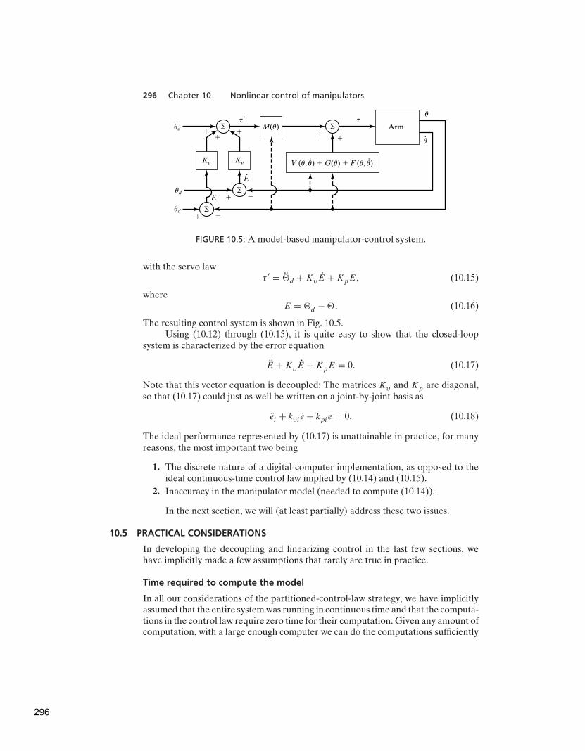
296 Chapter 10 Nonlinear control of manipulators
�
�
�
M(u)
Kp Ky
�
�
�
�
�
� ��
tt�
��
ud
..
ud
.
ud
u.
u
Arm
V (u, u) � G(u) � F (u, u). .
E.
E
FIGURE 10.5: A model-based manipulator-control system.
with the servo lawτ ′ = d +KυE +KpE, (10.15)
whereE = d − . (10.16)
The resulting control system is shown in Fig. 10.5.Using (10.12) through (10.15), it is quite easy to show that the closed-loop
system is characterized by the error equation
E +KυE +KpE = 0. (10.17)
Note that this vector equation is decoupled: The matrices Kυ and Kp are diagonal,so that (10.17) could just as well be written on a joint-by-joint basis as
ei + kυi e + kpie = 0. (10.18)
The ideal performance represented by (10.17) is unattainable in practice, for manyreasons, the most important two being
1. The discrete nature of a digital-computer implementation, as opposed to theideal continuous-time control law implied by (10.14) and (10.15).
2. Inaccuracy in the manipulator model (needed to compute (10.14)).
In the next section, we will (at least partially) address these two issues.
10.5 PRACTICAL CONSIDERATIONS
In developing the decoupling and linearizing control in the last few sections, wehave implicitly made a few assumptions that rarely are true in practice.
Time required to compute the model
In all our considerations of the partitioned-control-law strategy, we have implicitlyassumed that the entire system was running in continuous time and that the computa-tions in the control law require zero time for their computation. Given any amount ofcomputation, with a large enough computer we can do the computations sufficiently
296

Section 10.5 Practical considerations 297
fast that this is a reasonable approximation; however, the expense of the computercould make the scheme economically unfeasible. In the manipulator-control case,the entire dynamic equation of the manipulator, (10.14), must be computed in thecontrol law. These computations are quite involved; consequently, as was discussedin Chapter 6, there has been a great deal of interest in developing fast computationalschemes to compute them in an efficient way. As computer power becomes more andmore affordable, control laws that require a great deal of computation will becomemore practical. Several experimental implementations of nonlinear-model-basedcontrol laws have been reported [5–9], and partial implementations are beginningto appear in industrial controllers.
As was discussed in Chapter 9, almost all manipulator-control systems arenow performed in digital circuitry and are run at a certain sampling rate. Thismeans that the position (and possibly other) sensors are read at discrete pointsin time. From the values read, an actuator command is computed and sent tothe actuator. Thus, reading sensors and sending actuator commands are not donecontinuously, but rather at a finite sampling rate. To analyze the effect of delaydue to computation and finite sample rate, we must use tools from the field ofdiscrete-time control. In discrete time, differential equations turn into differenceequations, and a complete set of tools has been developed to answer questionsabout stability and pole placement for these systems. Discrete-time control theoryis beyond the scope of this book, although, for researchers working in the area ofmanipulator control, many of the concepts from discrete-time systems are essential.(See [10].)
Although important, ideas and methods from discrete-time control theoryare often difficult to apply to the case of nonlinear systems. Whereas we havemanaged to write a complicated differential equation of motion for the manipulatordynamic equation, a discrete-time equivalent is impossible to obtain in generalbecause, for a general manipulator, the only way to solve for the motion of themanipulator for a given set of initial conditions, an input, and a finite interval is bynumerical integration (as we saw in Chapter 6). Discrete-time models are possibleif we are willing to use series solutions to the differential equations, or if we makeapproximations. However, if we need to make approximations to develop a discretemodel, then it is not clear whether we have a better model than we have when justusing the continuous model and making the continuous-time approximation. Sufficeit to say that analysis of the discrete-time manipulator-control problem is difficult,and usually simulation is resorted to in order to judge the effect that a certain samplerate will have on performance.
We will generally assume that the computations can be performed quicklyenough and often enough that the continuous-time approximation is valid.
Feedforward nonlinear control
The use of feedforward control has been proposed as a method of using a nonlineardynamic model in a control law without the need for complex and time-consumingcomputations to be performed at servo rates [11]. In Fig. 10.5, the model-basedcontrol portion of the control law is ‘‘in the servo loop’’ in that signals ‘‘flow’’through that black box with each tick of the servo clock. If we wish to select a sample
297

298 Chapter 10 Nonlinear control of manipulators
�
�
�
Kp Ky
�
�
�
�
�
� �
t
E.
E
Arm
u.
u�Dynamic
Modelud
ud
..
ud
.
FIGURE 10.6: Control scheme with the model-based portion ‘‘outside’’ the servoloop.
rate of 200 Hz, then the dynamic model of the manipulator must be computed at thisrate. Another possible control system is shown in Fig. 10.6. Here, the model-basedcontrol is ‘‘outside’’ the servo loop. Hence, it is possible to have a fast inner servoloop, consisting simply of multiplying errors by gains, with the model-based torquesadded at a slower rate.
Unfortunately, the feedforward scheme of Fig. 10.6 does not provide completedecoupling. If we write the system equations,1 we will find that the error equationof this system is
E +M−1( )KυE +M−1( )KpE = 0. (10.19)
Clearly, as the configuration of the arm changes, the effective closed-loop gainchanges, and the quasi-static poles move around in the real–imaginary plane.However, equation (10.19) could be used as a starting point for designing a robustcontroller—one that finds a good set of constant gains such that, despite the‘‘motion’’ of the poles, they are guaranteed to remain in reasonably favorablelocations. Alternatively, one might consider schemes in which variable gains areprecomputed which change with configuration of the robot, so that the system’squasi-static poles remain in fixed positions.
Note that, in the system of Fig. 10.6, the dynamic model is computed as afunction of the desired path only, so when the desired path is known in advance,values could be computed ‘‘off-line’’ before motion begins. At run time, theprecomputed torque histories would then be read out of memory. Likewise, if time-varying gains are computed, they too could be computed beforehand and stored.Hence, such a scheme could be quite inexpensive computationally at run time andthus achieve a high servo rate.
Dual-rate computed-torque implementation
Figure 10.7 shows the block diagram of a possible practical implementation of thedecoupling and linearizing position-control system. The dynamic model is expressedin its configuration space form so that the dynamic parameters of the manipulatorwill appear as functions of manipulator position only. These functions might then
1We have used the simplifying assumptionsM( d )∼= M( ), V ( d , d ) ∼= (V ( , ),G( d ) ∼= G( ),
and F( d , d )∼= F( , ).
298

Section 10.5 Practical considerations 299
�
�
�
Kp Ky
�
�
�
�
�
� � �
�t
u
��
Arm
ud
ud
..
ud
.
M (u) u.
B (u) � C (u)
G (u)
FIGURE 10.7: An implementation of the model-based manipulator-control system.
be computed by a background process or by a second control computer [8] or belooked up in a precomputed table [12]. In this architecture, the dynamic parameterscan be updated at a rate slower than the rate of the closed-loop servo. For example,the background computation might proceed at 60 Hz while the closed-loop servowas running at 250 Hz.
Lack of knowledge of parameters
The second potential difficulty encountered in employing the computed-torquecontrol algorithm is that the manipulator dynamic model is often not knownaccurately. This is particularly true of certain components of the dynamics, suchas friction effects. In fact, it is usually extremely difficult to know the structure ofthe friction model, let alone the parameter values [13]. Finally, if the manipulatorhas some portion of its dynamics that is not repeatable—because, for example, itchanges as the robot ages—it is difficult to have good parameter values in the modelat all times.
By nature, most robots will be picking up various parts and tools. When arobot is holding a tool, the inertia and the weight of the tool change the dynamicsof the manipulator. In an industrial situation, the mass properties of the tools mightbe known—in this case, they can be accounted for in the modeled portion of thecontrol law. When a tool is grasped, the inertia matrix, total mass, and center ofmass of the last link of the manipulator can be updated to new values that representthe combined effect of the last link plus tool. However, in many applications, themass properties of objects that the manipulator picks up are not generally known,so maintenance of an accurate dynamic model is difficult.
The simplest possible nonideal situation is one in which we still assume aperfect model implemented in continuous time, but with external noise acting todisturb the system. In Fig. 10.8, we indicate a vector of disturbance torques actingat the joints. Writing the system error equation with inclusion of these unknowndisturbances, we arrive at
E +KυE +KpE = M−1( )τd , (10.20)
299

300 Chapter 10 Nonlinear control of manipulators
�
�
�
Kp Ky
�
�
�
�
�
� � �
�
�t
td
u
��
Arm
ud
ud
..
ud
.
M (u) u.
B (u) � C (u)
G (u)
FIGURE 10.8: The model-based controller with an external disturbance acting.
where τd is the vector of disturbance torques at the joints. The left-hand side of(10.20) is uncoupled, but, from the right-hand side, we see that a disturbance on anyparticular joint will introduce errors at all the other joints, becauseM ( ) is not, ingeneral, diagonal.
Some simple analyses might be performed on the basis of (10.20). For example,it is easy to compute the steady-state servo error due to a constant disturbance as
E = K−1pM−1( )τd . (10.21)
When our model of the manipulator dynamics is not perfect, analysis ofthe resulting closed-loop system becomes more difficult. We define the followingnotation: M( ) is our model of the manipulator inertia matrix, M ( ). Likewise,V ( , ), G( ), and F ( , ) are our models of the velocity terms, gravity terms,and friction terms of the actual mechanism. Perfect knowledge of the modelwould mean that
M( ) = M( ),V ( , ) = V ( , ), (10.22)
G( ) = G( ),F ( , ) = F( , ).
Therefore, although the manipulator dynamics are given by
τ = M( ) + V ( , )+G( )+ F( , ), (10.23)
our control law computes
τ = ατ ′ + β,α = M( ), (10.24)
β = V ( , )+ G( )+ F ( , ).
300

Section 10.6 Current industrial-robot control systems 301
Decoupling and linearizing will not, therefore, be perfectly accomplished whenparameters are not known exactly. Writing the closed-loop equation for the system,we have
E +Kυ E +KpE
= M−1[(M − M) + (V − V )+ (G− G)+ (F − F )], (10.25)
where the arguments of the dynamic functions are not shown for brevity. Note that,if the model were exact, so that (10.22) were true, then the right-hand side of (10.25)would be zero and the errors would disappear. When the parameters are not knownexactly, the mismatch between actual and modeled parameters will cause servoerrors to be excited (possibly even resulting in an unstable system [21]) according tothe rather complicated equation (10.25).
Discussion of stability analysis of a nonlinear closed-loop system is deferreduntil Section 10.7.
10.6 CURRENT INDUSTRIAL-ROBOT CONTROL SYSTEMS
Because of the problems with having good knowledge of parameters, it is not clearwhether it makes sense to go to the trouble of computing a complicated model-basedcontrol law for manipulator control. The expense of the computer power needed tocompute the model of the manipulator at a sufficient rate might not be worthwhile,especially when lack of knowledge of parameters could nullify the benefits of such anapproach. Manufacturers of industrial robots have decided, probably for economicreasons, that attempting to use a complete manipulator model in the controller isnot worthwhile. Instead, present-day manipulators are controlled with very simplecontrol laws that generally are completely error driven and are implemented inarchitectures such as those studied in Section 9.10. An industrial robot with ahigh-performance servo system is shown in Fig. 10.9.
Individual-joint PID control
Most industrial robots nowadays have a control scheme that, in our notation, wouldbe described by
α = I,β = 0, (10.26)
where I is the n× n identity matrix. The servo portion is
τ ′ = d +KυE +KpE +Ki∫
Edt, (10.27)
where Kυ , Kp, and Ki are constant diagonal matrices. In many cases, d is notavailable, and this term is simply set to zero. That is, most simple robot controllersdo not use a model-based component at all in their control law. This type of PIDcontrol scheme is simple because each joint is controlled as a separate controlsystem. Often, one microprocessor per joint is used to implement (10.27), as wasdiscussed in Section 9.10.
301
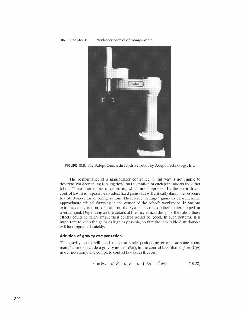
302 Chapter 10 Nonlinear control of manipulators
FIGURE 10.9: The Adept One, a direct-drive robot by Adept Technology, Inc.
The performance of a manipulator controlled in this way is not simple todescribe. No decoupling is being done, so the motion of each joint affects the otherjoints. These interactions cause errors, which are suppressed by the error-drivencontrol law. It is impossible to select fixed gains that will critically damp the responseto disturbances for all configurations. Therefore, ‘‘average’’ gains are chosen, whichapproximate critical damping in the center of the robot’s workspace. In variousextreme configurations of the arm, the system becomes either underdamped oroverdamped. Depending on the details of the mechanical design of the robot, theseeffects could be fairly small; then control would be good. In such systems, it isimportant to keep the gains as high as possible, so that the inevitable disturbanceswill be suppressed quickly.
Addition of gravity compensation
The gravity terms will tend to cause static positioning errors, so some robotmanufacturers include a gravity model, G(θ), in the control law (that is, β = G( )
in our notation). The complete control law takes the form
τ ′ = d +Kυ E +KpE +Ki∫
Edt + G( ). (10.28)
302

Section 10.7 Lyapunov stability analysis 303
Such a control law is perhaps the simplest example of a model-based controller.Because (10.28) can no longer be implemented on a strict joint-by-joint basis, thecontroller architecture must allow communication between the joint controllers ormust make use of a central processor rather than individual-joint processors.
Various approximations of decoupling control
There are various ways to simplify the dynamic equations of a particular manipulator[3,14]. After the simplification, an approximate decoupling and linearizing law canbe derived. A usual simplification might be to disregard components of torquedue to the velocity terms—that is, to model only the inertial and gravity terms.Often, friction models are not included in the controller, because friction is so hardto model correctly. Sometimes, the inertia matrix is simplified so that it accountsfor the major coupling between axes but not for minor cross-coupling effects. Forexample, [14] presents a simplified version of the PUMA 560’s mass matrix thatrequires only about 10% of the calculations needed to compute the complete massmatrix, yet is accurate to within 1%.
10.7 LYAPUNOV STABILITY ANALYSIS
In Chapter 9, we examined linear control systems analytically to evaluate stabilityand also performance of the dynamic response in terms of damping and closed-loop bandwidth. The same analyses are valid for a nonlinear system that has beendecoupled and linearized by means of a perfect model-based nonlinear controller,because the overall resulting system is again linear. However, when decoupling andlinearizing are not performed by the controller, or are incomplete or inaccurate,the overall closed-loop system remains nonlinear. For nonlinear systems, stabilityand performance analysis is much more difficult. In this section, we introduce onemethod of stability analysis that is applicable to both linear and nonlinear systems.
Consider the simple mass–spring friction system originally introduced inChapter 9, whose equation of motion is
mx + bx + kx = 0. (10.29)
The total energy of the system is given by
υ = 1
2mx2 + 1
2kx2, (10.30)
where the first term gives the kinetic energy of the mass and the second term givesthe potential energy stored in the spring. Note that the value, υ, of the system energyis always nonnegative (i.e., it is positive or zero). Let’s find out the rate of change ofthe total energy by differentiating (10.30) with respect to time, to obtain
υ = mxx + kxx. (10.31)
Substituting (10.29) for mx in (10.31) yields
υ = −bx2, (10.32)
which we note is always nonpositive (because b > 0). Thus, energy is always leavingthe system, unless x = 0. This implies that, however initially perturbed, the system
303

304 Chapter 10 Nonlinear control of manipulators
will lose energy until it comes to rest. Investigating possible resting positions bymeans of a steady-state analysis of (10.29) yields
kx = 0, (10.33)
orx = 0. (10.34)
Hence, by means of an energy analysis, we have shown that the system of (10.29)with any initial conditions (i.e., any initial energy) will eventually come to restat the equilibrium point. This stability proof by means of an energy analysis is asimple example of a more general technique called Lyapunov stability analysis orLyapunov’s second (or direct) method, after a Russian mathematician of the 19thcentury [15].
An interesting feature of this method of stability analysis is that we can concludestability without solving for the solution of the differential equation governingthe system. However, while Lyapunov’s method is useful for examining stability,it generally does not provide any information about the transient response orperformance of the system. Note that our energy analysis yielded no information onwhether the system was overdamped or underdamped or on how long it would takethe system to suppress a disturbance. It is important to distinguish between stabilityand performance: A stable system might nonetheless exhibit control performanceunsatisfactory for its intended use.
Lyapunov’s method is somewhat more general than our example indicated.It is one of the few techniques that can be applied directly to nonlinear systemsto investigate their stability. As a means of quickly getting an idea of Lyapunov’smethod (in sufficient detail for our needs), we will look at an extremely briefintroduction to the theory and then proceed directly to several examples. A morecomplete treatment of Lyapunov theory can be found in [16, 17].
Lyapunov’s method is concerned with determining the stability of a differentialequation
X = f (X), (10.35)
where X is m × 1 and f (·) could be nonlinear. Note that higher order differentialequations can always be written as a set of first-order equations in the form (10.35).To prove a system stable by Lyapunov’s method, one is required to propose ageneralized energy function υ(X) that has the following properties:
1. υ(X) has continuous first partial derivatives, and υ(X) > 0 for all X exceptυ(0) = 0.
2. υ(X) ≤ 0. Here, υ(X)means the change in υ(X) along all system trajectories.
These properties might hold only in a certain region, or they might be global,with correspondingly weaker or stronger stability results. The intuitive idea is thata positive definite ‘‘energy-like’’ function of state is shown to always decrease orremain constant—hence, the system is stable in the sense that the size of the statevector is bounded.
When υ(X) is strictly less than zero, asymptotic convergence of the state tothe zero vector can be concluded. Lyapunov’s original work was extended in an
304
Section 10.7 Lyapunov stability analysis 305
important way by LaSalle and Lefschetz [4], who showed that, in certain situations,even when υ(X) ≤ 0 (note equality included), asymptotic stability can be shown.For our purposes, we can deal with the case υ(X) = 0 by performing a steady-stateanalysis in order to learn whether the stability is asymptotic or the system understudy can ‘‘get stuck’’ somewhere other than υ(X) = 0.
A system described by (10.35) is said to be autonomous because the func-tion f (·) is not an explicit function of time. Lyapunov’s method also extends tononautonomous systems, in which time is an argument of the nonlinear function.See [4, 17] for details.
EXAMPLE 10.4
Consider the linear system
X = −AX, (10.36)
where A is m×m and positive definite. Propose the candidate Lyapunov function
υ(X) = 1
2XTX, (10.37)
which is continuous and everywhere nonnegative. Differentiating yields
υ(X) = XT X= XT (−AX) (10.38)
= −XTAX,
which is everywhere nonpositive because A is a positive definite matrix. Hence,(10.37) is indeed a Lyapunov function for the system of (10.36). The system isasymptotically stable because υ(X) can be zero only at X = 0; everywhere else, Xmust decrease.
EXAMPLE 10.5
Consider a mechanical spring–damper system in which both the spring and damperare nonlinear:
x + b(x)+ k(x) = 0. (10.39)
The functions b(·) and k(·) are first- and third-quadrant continuous functionssuch that
xb(x) > 0 f or x �= 0,
xk(x) > 0 f or x �= 0. (10.40)
Once having proposed the Lyapunov function
υ(x, x) = 1
2x2 +
∫ x
0k(λ)dλ, (10.41)
305

306 Chapter 10 Nonlinear control of manipulators
we are led to
υ(x, x) = xx + k(x)x,= −xb(x)− k(x)x + k(x)x, (10.42)
= −xb(x).
Hence, υ(·) is nonpositive but is only semidefinite, because it is not a function of xbut only of x. In order to conclude asymptotic stability, we have to ensure that it isnot possible for the system to ‘‘get stuck’’ with nonzero x. To study all trajectoriesfor which x = 0, we must consider
x = −k(x), (10.43)
for which x = 0 is the only solution. Hence, the system will come to rest only ifx = x = x = 0.
EXAMPLE 10.6
Consider a manipulator with dynamics given by
τ = M( ) + V ( , )+G( ) (10.44)
and controlled with the control law
τ = KpE −Kd +G( ), (10.45)
whereKp andKd are diagonal gain matrices. Note that this controller does not forcethe manipulator to follow a trajectory, but moves the manipulator to a goal pointalong a path specified by the manipulator dynamics and then regulates the positionthere. The resulting closed-loop system obtained by equating (10.44) and (10.45) is
M( ) + V ( , )+Kd +Kp = Kp d ; (10.46)
it can be proven globally asymptotically stable by Lyapunov’s method [18, 19].Consider the candidate Lyapunov function
υ = 1
2 TM( ) + 1
2ETKpE. (10.47)
The function (10.47) is always positive or zero, because the manipulator massmatrix, M( ), and the position gain matrix, Kp, are positive definite matrices.Differentiating (10.47) yields
υ = 1
2 T M( )θ + θTM(θ) − ETKp
= 1
2 T M( ) − TKd − T V ( , ) (10.48)
= − TKd ,
306

Section 10.8 Cartesian-based control systems 307
which is nonpositive as long as Kd is positive definite. In taking the last step in(10.48), we have made use of the interesting identity
1
2 T M( ) = T V ( , ), (10.49)
which can be shown by investigation of the structure of Lagrange’s equations ofmotion [18–20]. (See also Exercise 6.17.)
Next, we investigate whether the system can get ‘‘stuck’’ with nonzero error.Because υ can remain zero only along trajectories that have = 0 and = 0, wesee from (10.46) that, in this case,
KpE = 0, (10.50)
and because Kp is nonsingular, we have
E = 0. (10.51)
Hence, control law (10.45) applied to the system (10.44) achieves global asymptoticstability.
This proof is important in that it explains, to some extent, why today’s industrialrobots work. Most industrial robots use a simple error-driven servo, occasionallywith gravity models, and so are quite similar to (10.45).
See Exercises 10.11 through 10.16 for more examples of nonlinear manipulator-control laws that can be proven stable by Lyapunov’s method. Recently, Lyapunovtheory has become increasingly prevalent in robotics research publications [18–25].
10.8 CARTESIAN-BASED CONTROL SYSTEMS
In this section, we introduce the notion of Cartesian-based control. Although suchapproaches are not currently used in industrial robots, there is activity at severalresearch institutions on such schemes.
Comparison with joint-based schemes
In all the control schemes for manipulators we have discussed so far, we assumedthat the desired trajectory was available in terms of time histories of joint position,velocity, and acceleration. Given that these desired inputs were available, wedesigned joint-based control schemes, that is, schemes in which we develop trajectoryerrors by finding the difference between desired and actual quantities expressed injoint space. Very often, we wish the manipulator end-effector to follow straight linesor other path shapes described in Cartesian coordinates. As we saw in Chapter 7, itis possible to compute the time histories of the joint-space trajectory that correspondto Cartesian straight-line paths. Figure 10.10 shows this approach to manipulator-trajectory control. A basic feature of the approach is the trajectory-conversionprocess, which is used to compute the joint trajectories. This is then followed bysome kind of joint-based servo scheme such as we have been studying.
307
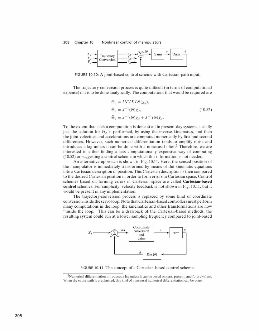
308 Chapter 10 Nonlinear control of manipulators
TrajectoryConversion
GainsXd
Xd
Xd
ud
du u
� �ud
ud
Armt
a
FIGURE 10.10: A joint-based control scheme with Cartesian-path input.
The trajectory-conversion process is quite difficult (in terms of computationalexpense) if it is to be done analytically. The computations that would be required are
d = INVKIN(χd),
d = J−1( )χd , (10.52)
d = J−1( )χd + J−1( )χd .
To the extent that such a computation is done at all in present-day systems, usuallyjust the solution for d is performed, by using the inverse kinematics, and thenthe joint velocities and accelerations are computed numerically by first and seconddifferences. However, such numerical differentiation tends to amplify noise andintroduces a lag unless it can be done with a noncausal filter.2 Therefore, we areinterested in either finding a less computationally expensive way of computing(10.52) or suggesting a control scheme in which this information is not needed.
An alternative approach is shown in Fig. 10.11. Here, the sensed position ofthe manipulator is immediately transformed by means of the kinematic equationsinto a Cartesian description of position. This Cartesian description is then comparedto the desired Cartesian position in order to form errors in Cartesian space. Controlschemes based on forming errors in Cartesian space are called Cartesian-basedcontrol schemes. For simplicity, velocity feedback is not shown in Fig. 10.11, but itwould be present in any implementation.
The trajectory-conversion process is replaced by some kind of coordinateconversion inside the servo loop. Note that Cartesian-based controllers must performmany computations in the loop; the kinematics and other transformations are now‘‘inside the loop.’’ This can be a drawback of the Cartesian-based methods; theresulting system could run at a lower sampling frequency compared to joint-based
Coordinateconversion
andgains
Xd
dX
X
ua
� �
Armt
Kin (u)
FIGURE 10.11: The concept of a Cartesian-based control scheme.
2Numerical differentiation introduces a lag unless it can be based on past, present, and future values.When the entire path is preplanned, this kind of noncausal numerical differentiation can be done.
308

Section 10.8 Cartesian-based control systems 309
systems (given the same size of computer). This would, in general, degrade thestability and disturbance-rejection capabilities of the system.
Intuitive schemes of Cartesian control
One possible control scheme that comes to mind rather intuitively is shown inFig. 10.12. Here, Cartesian position is compared to the desired position to forman error, δX, in Cartesian space. This error, which may be presumed small if thecontrol system is doing its job, may be mapped into a small displacement in jointspace by means of the inverse Jacobian. The resulting errors in joint space, δθ , arethen multiplied by gains to compute torques that will tend to reduce these errors.Note that Fig. 10.12 shows a simplified controller in which, for clarity, the velocityfeedback has not been shown. It could be added in a straightforward manner. Wewill call this scheme the inverse-Jacobian controller.
Another scheme which could come to mind is shown in Fig. 10.13. Here, theCartesian error vector is multiplied by a gain to compute a Cartesian force vector.This can be thought of as a Cartesian force which, if applied to the end-effectorof the robot, would push the end-effector in a direction that would tend to reducethe Cartesian error. This Cartesian force vector (actually a force–moment vector)is then mapped through the Jacobian transpose in order to compute the equivalentjoint torques that would tend to reduce the observed errors. We will call this schemethe transpose-Jacobian controller.
The inverse-Jacobian controller and the transpose-Jacobian controller haveboth been arrived at intuitively. We cannot be sure that such arrangements wouldbe stable, let alone perform well. It is also curious that the schemes are extremelysimilar, except that the one contains the Jacobian’s inverse, the other its transpose.Remember, the inverse is not equal to the transpose in general (only in the case ofa strictly Cartesian manipulator does J T = J−1). The exact dynamic performance
Xd
dX
X
ua
� �
Armt
Gainsdu
J�1
Kin (u)
FIGURE 10.12: The inverse-Jacobian Cartesian-control scheme.
Xd
dX
X
u
� �
ArmtF
Gains JT
Kin (u)
a
FIGURE 10.13: The transpose-Jacobian Cartesian-control scheme.
309

310 Chapter 10 Nonlinear control of manipulators
of such systems (if expressed in a second-order error-space equation, for example)is very complicated. It turns out that both schemes will work (i.e., can be madestable), but not well (i.e., performance is not good over the entire workspace). Bothcan be made stable by appropriate gain selection, including some form of velocityfeedback (which was not shown in Figs. 10.12 and 10.13). While both will work,neither is correct, in the sense that we cannot choose fixed gains that will result infixed closed-loop poles. The dynamic response of such controllers will vary with armconfiguration.
Cartesian decoupling scheme
For Cartesian-based controllers, like joint-based controllers, good performancewould be characterized by constant error dynamics over all configurations of themanipulator. Errors are expressed in Cartesian space in Cartesian-based schemes,so this means that we would like to design a system which, over all possibleconfigurations, would suppress Cartesian errors in a critically damped fashion.
Just as we achieved good control with a joint-based controller that was basedon a linearizing and decoupling model of the arm, we can do the same for theCartesian case. However, we must now write the dynamic equations of motion ofthe manipulator in terms of Cartesian variables. This can be done, as was discussedin Chapter 6. The resulting form of the equations of motion is quite analogous tothe joint-space version. The rigid-body dynamics can be written as
F = Mx( )χ + Vx( , )+Gx( ), (10.53)
where F is a fictitious force–moment vector acting on the end-effector of the robotand χ is an appropriate Cartesian vector representing position and orientation ofthe end-effector [8]. Analogous to the joint-space quantities, Mx( ) is the massmatrix in Cartesian space, Vx( , ) is a vector of velocity terms in Cartesian space,and Gx( ) is a vector of gravity terms in Cartesian space.
Just as we did in the joint-based case, we can use the dynamic equations ina decoupling and linearizing controller. Because (10.53) computes F , a fictitiousCartesian force vector which should be applied to the hand, we will also need to usethe transpose of the Jacobian in order to implement the control—that is, after F iscalculated by (10.53), we cannot actually cause a Cartesian force to be applied tothe end-effector; we instead compute the joint torques needed to effectively balancethe system if we were to apply this force:
τ = J T ( )F . (10.54)
Figure 10.14 shows a Cartesian arm-control system using complete dynamicdecoupling. Note that the arm is preceded by the Jacobian transpose. Notice thatthe controller of Fig. 10.14 allows Cartesian paths to be described directly, with noneed for trajectory conversion.
As in the joint-space case, a practical implementation might best be achievedthrough use of a dual-rate control system. Figure 10.15 shows a block diagramof a Cartesian-based decoupling and linearizing controller in which the dynamicparameters are written as functions of manipulator position only. These dynamicparameters are updated at a rate slower than the servo rate by a background
310

Section 10.9 Adaptive control 311
� �
� �
Armt
Mx(u) JT(u)
Kp
E
Kv
Kin (u)uXd
xd
x
x
xd
E
J(u)
u
Vx(u,u) � Gx(u)
a a
a
a
FIGURE 10.14: The Cartesian model-based control scheme.
a
a
a
Kv
Kp
G (u)
Bx(u) � Cx(u)
Mx(u) JT(u)
t
Arm
uKin (u)
J(u)
�xd
xd
xd
u
x
EE
� �
� �
x
FIGURE 10.15: An implementation of the Cartesian model-based control scheme.
process or a second control computer. This is appropriate, because we desire a fastservo (perhaps running at 500 Hz or even higher) to maximize disturbance rejectionand stability. The dynamic parameters are functions of manipulator position only,so they need be updated at a rate related only to how fast the manipulator ischanging configuration. The parameter-update rate probably need not be higherthan 100 Hz [8].
10.9 ADAPTIVE CONTROL
In the discussion of model-based control, it was noted that, often, parameters ofthe manipulator are not known exactly. When the parameters in the model do not
311
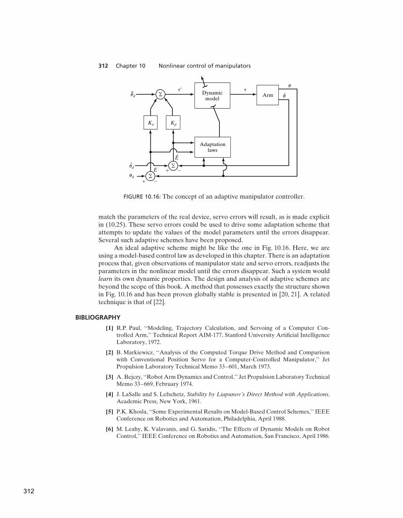
312 Chapter 10 Nonlinear control of manipulators
Ky Kp
�� �
Adaptationlaws
Dynamicmodel
Armud
ud
ud
u
u
E
E
a
a
a
� �
� �
FIGURE 10.16: The concept of an adaptive manipulator controller.
match the parameters of the real device, servo errors will result, as is made explicitin (10.25). These servo errors could be used to drive some adaptation scheme thatattempts to update the values of the model parameters until the errors disappear.Several such adaptive schemes have been proposed.
An ideal adaptive scheme might be like the one in Fig. 10.16. Here, we areusing a model-based control law as developed in this chapter. There is an adaptationprocess that, given observations of manipulator state and servo errors, readjusts theparameters in the nonlinear model until the errors disappear. Such a system wouldlearn its own dynamic properties. The design and analysis of adaptive schemes arebeyond the scope of this book. A method that possesses exactly the structure shownin Fig. 10.16 and has been proven globally stable is presented in [20, 21]. A relatedtechnique is that of [22].
BIBLIOGRAPHY
[1] R.P. Paul, ‘‘Modeling, Trajectory Calculation, and Servoing of a Computer Con-trolled Arm,’’ Technical Report AIM-177, Stanford University Artificial IntelligenceLaboratory, 1972.
[2] B. Markiewicz, ‘‘Analysis of the Computed Torque Drive Method and Comparisonwith Conventional Position Servo for a Computer-Controlled Manipulator,’’ JetPropulsion Laboratory Technical Memo 33–601, March 1973.
[3] A. Bejczy, ‘‘Robot Arm Dynamics and Control,’’ Jet Propulsion Laboratory TechnicalMemo 33–669, February 1974.
[4] J. LaSalle and S. Lefschetz, Stability by Liapunov’s Direct Method with Applications,Academic Press, New York, 1961.
[5] P.K. Khosla, ‘‘Some Experimental Results on Model-Based Control Schemes,’’ IEEEConference on Robotics and Automation, Philadelphia, April 1988.
[6] M. Leahy, K. Valavanis, and G. Saridis, ‘‘The Effects of Dynamic Models on RobotControl,’’ IEEE Conference on Robotics and Automation, San Francisco, April 1986.
312
Bibliography 313
[7] L. Sciavicco and B. Siciliano, Modelling and Control of Robot Manipulators, 2ndEdition, Springer-Verlag, London, 2000.
[8] O. Khatib, ‘‘A Unified Approach for Motion and Force Control of Robot Manipula-tors: The Operational Space Formulation,’’ IEEE Journal of Robotics and Automation,Vol. RA-3, No. 1, 1987.
[9] C. An, C. Atkeson, and J. Hollerbach, ‘‘Model-Based Control of a Direct Drive Arm,Part II: Control,’’ IEEE Conference on Robotics and Automation, Philadelphia, April1988.
[10] G. Franklin, J. Powell, and M. Workman, Digital Control of Dynamic Systems, 2ndedition, Addison-Wesley, Reading, MA, 1989.
[11] A. Liegeois, A. Fournier, and M. Aldon, ‘‘Model Reference Control of High VelocityIndustrial Robots,’’ Proceedings of the Joint Automatic Control Conference, SanFrancisco, 1980.
[12] M. Raibert, ‘‘Mechanical Arm Control Using a State Space Memory,’’ SME paperMS77-750, 1977.
[13] B. Armstrong, ‘‘Friction: Experimental Determination, Modeling and Compensa-tion,’’ IEEE Conference on Robotics and Automation, Philadelphia, April 1988.
[14] B. Armstrong, O. Khatib, and J. Burdick, ‘‘The Explicit Dynamic Model and InertialParameters of the PUMA 560 Arm,’’ IEEE Conference on Robotics and Automation,San Francisco, April 1986.
[15] A.M. Lyapunov, ‘‘On the General Problem of Stability of Motion,’’ (in Russian),Kharkov Mathematical Society, Soviet Union, 1892.
[16] C. Desoer and M. Vidyasagar, Feedback Systems: Input–Output Properties, AcademicPress, New York, 1975.
[17] M. Vidyasagar, Nonlinear Systems Analysis, Prentice-Hall, Englewood Cliffs, NJ, 1978.
[18] S. Arimoto and F. Miyazaki, ‘‘Stability and Robustness of PID Feedback Controlfor Robot Manipulators of Sensory Capability,’’ Third International Symposium ofRobotics Research, Gouvieux, France, July 1985.
[19] D. Koditschek, ‘‘Adaptive Strategies for the Control of Natural Motion,’’ Proceedings
of the 24th Conference on Decision and Control, Ft. Lauderdale, FL, December 1985.
[20] J. Craig, P. Hsu, and S. Sastry, ‘‘Adaptive Control of Mechanical Manipulators,’’ IEEEConference on Robotics and Automation, San Francisco, April 1986.
[21] J. Craig, Adaptive Control of Mechanical Manipulators, Addison-Wesley, Reading,MA, 1988.
[22] J.J. Slotine and W. Li, ‘‘On the Adaptive Control of Mechanical Manipulators,’’ The
International Journal of Robotics Research, Vol. 6, No. 3, 1987.
[23] R. Kelly and R. Ortega, ‘‘Adaptive Control of Robot Manipulators: An Input–OutputApproach,’’ IEEE Conference on Robotics and Automation, Philadelphia, 1988.
[24] H. Das, J.J. Slotine, and T. Sheridan, ‘‘Inverse Kinematic Algorithms for RedundantSystems,’’ IEEE Conference on Robotics and Automation, Philadelphia, 1988.
[25] T. Yabuta, A. Chona, and G. Beni, ‘‘On the Asymptotic Stability of the HybridPosition/Force Control Scheme for Robot Manipulators,’’ IEEE Conference onRobotics and Automation, Philadelphia, 1988.
313

314 Chapter 10 Nonlinear control of manipulators
EXERCISES
10.1 [15] Give the nonlinear control equations for an α,β-partitioned controller forthe system
τ = (2√θ + 1)θ + 3θ2 − sin(θ).
Choose gains so that this system is always critically damped with kCL = 10.10.2 [15] Give the nonlinear control equations for an α,β-partitioned controller for
the systemτ = 5θθ + 2θ − 13θ3 + 5.
Choose gains so that this system is always critically damped with kCL = 10.10.3 [19] Draw a block diagram showing a joint-space controller for the two-link arm
from Section 6.7, such that the arm is critically damped over its entire workspace.Show the equations inside the blocks of a block diagram.
10.4 [20] Draw a block diagram showing a Cartesian-space controller for the two-link arm from Section 6.7, such that the arm is critically damped over its entireworkspace. (See Example 6.6.) Show the equations inside the blocks of a blockdiagram.
10.5 [18] Design a trajectory-following control system for the system whose dynamicsare given by
τ1 = m1l21θ1 +m1l1l2θ1θ2,
τ2 = m2l22(θ1 + θ2)+ υ2θ2.
Do you think these equations could represent a real system?10.6 [17] For the control system designed for the one-link manipulator in Example
10.3, give an expression for the steady-state position error as a function of errorin the mass parameter. Let ψm = m − m. The result should be a function ofl, g, θ, ψm, m, and kp . For what position of the manipulator is this at a maximum?
10.7 [26] For the two-degree-of-freedom mechanical system of Fig. 10.17, design acontroller that can cause x1 and x2 to follow trajectories and suppress disturbancesin a critically damped fashion.
10.8 [30] Consider the dynamic equations of the two-link manipulator from Section 6.7in configuration-space form. Derive expressions for the sensitivity of the computed
k
x2
m2
m1
b2
b1
x1
FIGURE 10.17: Mechanical system with two degrees of freedom.
314
Exercises 315
torque value versus small deviations in . Can you say something about howoften the dynamics should be recomputed in a controller like that of Fig. 10.7 asa function of average joint velocities expected during normal operations?
10.9 [32] Consider the dynamic equations of the two-link manipulator from Example6.6 in Cartesian configuration-space form. Derive expressions for the sensitivity ofthe computed torque value versus small deviations in . Can you say somethingabout how often the dynamics should be recomputed in a controller like thatof Fig. 10.15 as a function of average joint velocities expected during normaloperations?
10.10 [15] Design a control system for the system
f = 5xx + 2x − 12.
Choose gains so that this system is always critically damped with a closed-loopstiffness of 20.
10.11 [20] Consider a position-regulation system that (without loss of generality)attempts to maintain d = 0. Prove that the control law
τ = −Kp −M( )Kυ +G( )
yields an asymptotically stable nonlinear system. You may take Kυ to be of theform Kυ = kυIn where kυ is a scalar and In is the n× n identity matrix. Hint: Thisis similar to example 10.6.
10.12 [20] Consider a position-regulation system that (without loss of generality)attempts to maintain d = 0. Prove that the control law
τ = −Kp − M( )Kυ +G( )
yields an asymptotically stable nonlinear system. You may take Kυ to be of theformKυ = kυIn where kυ is a scalar and In is the n×n identity matrix. The matrix
M( ) is a positive definite estimate of the manipulator mass matrix. Hint: This issimilar to example 10.6.
10.13 [25] Consider a position-regulation system that (without loss of generality)attempts to maintain d = 0. Prove that the control law
τ = −M( )[Kp +Kυ ] +G( )
yields an asymptotically stable nonlinear system. You may take Kυ to be of theform Kυ = kυIn where kυ is a scalar and In is the n× n identity matrix. Hint: Thisis similar to example 10.6.
10.14 [25] Consider a position-regulation system that (without loss of generality)attempts to maintain d = 0. Prove that the control law
τ = −M( )[Kp +Kυ ] +G( )
yields an asymptotically stable nonlinear system. You may take Kυ to be of theform Kυ = kυIn, where kυ is a scalar and In is the n × n identity matrix. The
matrix M( ) is a positive definite estimate of the manipulator mass matrix. Hint:This is similar to example 10.6.
10.15 [28] Consider a position-regulation system that (without loss of generality)attempts to maintain d = 0. Prove that the control law
τ = −Kp −Kυ
315
316 Chapter 10 Nonlinear control of manipulators
yields a stable nonlinear system. Show that stability is not asymptotic and give anexpression for the steady-state error. Hint: This is similar to Example 10.6.
10.16 [30] Prove the global stability of the Jacobian-transpose Cartesian controllerintroduced in Section 10.8. Use an appropriate form of velocity feedback tostabilize the system. Hint: See [18].
10.17 [15] Design a trajectory-following controller for a system with dynamics given by
f = ax2xx + bx2 + csin(x),
such that errors are suppressed in a critically damped fashion over all configura-tions.
10.18 [15] A system with open-loop dynamics given by
τ = mθ + bθ2 + cθ
is controlled with the control law
τ = m[θd + kυ e + kpe] + sin(θ).
Give the differential equation that characterizes the closed-loop action of thesystem.
PROGRAMMING EXERCISE (PART 10)
Repeat Programming Exercise Part 9, and use the same tests, but with a new controllerthat uses a complete dynamic model of the 3-link to decouple and linearize the system.For this case, use
Kp =
100.0 0.0 0.00.0 100.0 0.00.0 0.0 100.0
.
Choose a diagonal Kυ that guarantees critical damping over all configurations of thearm. Compare the results with those obtained with the simpler controller used inProgramming Exercise Part 9.
316
C H A P T E R 11
Force control of manipulators
11.1 INTRODUCTION
11.2 APPLICATION OF INDUSTRIAL ROBOTS TO ASSEMBLY TASKS
11.3 A FRAMEWORK FOR CONTROL IN PARTIALLY CONSTRAINED TASKS
11.4 THE HYBRID POSITION/FORCE CONTROL PROBLEM
11.5 FORCE CONTROL OF A MASS–SPRING SYSTEM
11.6 THE HYBRID POSITION/FORCE CONTROL SCHEME
11.7 CURRENT INDUSTRIAL-ROBOT CONTROL SCHEMES
11.1 INTRODUCTION
Position control is appropriate when a manipulator is following a trajectory throughspace, but when any contact is made between the end-effector and the manipulator’senvironment, mere position control might not suffice. Consider a manipulatorwashing a window with a sponge. The compliance of the sponge might make itpossible to regulate the force applied to the window by controlling the position ofthe end-effector relative to the glass. If the sponge is very compliant or the positionof the glass is known very accurately, this technique could work quite well.
If, however, the stiffness of the end-effector, tool, or environment is high,it becomes increasingly difficult to perform operations in which the manipulatorpresses against a surface. Instead of washing with a sponge, imagine that themanipulator is scraping paint off a glass surface, using a rigid scraping tool. If thereis any uncertainty in the position of the glass surface or any error in the positionof the manipulator, this task would become impossible. Either the glass would bebroken, or the manipulator would wave the scraping tool over the glass with nocontact taking place.
In both the washing and scraping tasks, it would be more reasonable not tospecify the position of the plane of the glass, but rather to specify a force that is to be
maintained normal to the surface.More so than in previous chapters, in this chapter we present methods that are
not yet employed by industrial robots, except in an extremely simplified way. Themajor thrust of the chapter is to introduce the hybrid position/force controller, whichis one formalism through which industrial robots might someday be controlled inorder to perform tasks requiring force control. However, regardless of whichmethod(s) emerge as practical for industrial application, many of the conceptsintroduced in this chapter will certainly remain valid.
From Chapter 11 of Introduction to Robotics: Mechanics and Control, Third Edition. John J. Craig.
Copyright © 2005 by Pearson Education, Inc. All rights reserved.
317

318 Chapter 11 Force control of manipulators
11.2 APPLICATION OF INDUSTRIAL ROBOTS TO ASSEMBLY TASKS
The majority of the industrial robot population is employed in relatively simpleapplications, such as spot welding, spray painting, and pick-and-place operations.Force control has already appeared in a few applications; for example, some robotsare already capable of simple force control that allows them to do such tasks asgrinding and deburring. Apparently, the next big area of application will be toassembly-line tasks in which one or more parts are mated. In such parts-matingtasks, monitoring and control of the forces of contact are extremely important.
Precise control of manipulators in the face of uncertainties and variations intheir work environments is a prerequisite to application of robot manipulators toassembly operations in industry. It seems that, by providing manipulator hands withsensors that can give information about the state of manipulation tasks, importantprogress can be made toward using robots for assembly tasks. Currently, thedexterity of manipulators remains quite low and continues to limit their applicationin the automated assembly area.
The use of manipulators for assembly tasks requires that the precision withwhich parts are positioned with respect to one another be quite high. Currentindustrial robots are often not accurate enough for these tasks, and building robotsthat are might not make sense. Manipulators of greater precision can be achievedonly at the expense of size, weight, and cost. The ability to measure and controlcontact forces generated at the hand, however, offers a possible alternative forextending the effective precision of a manipulation. Because relative measurementsare used, absolute errors in the position of the manipulator and the manipulatedobjects are not as important as they would be in a purely position-controlled system.Small variations in relative position generate large contact forces when parts ofmoderate stiffness interact, so knowledge and control of these forces can lead to atremendous increase in effective positional accuracy.
11.3 A FRAMEWORK FOR CONTROL IN PARTIALLY CONSTRAINED TASKS
The approach presented in this chapter is based on a framework for control insituations in which motion of the manipulator is partially constrained by contact withone or more surfaces [1–3]. This framework for understanding partially constrainedtasks is based on a simplified model of interaction between the manipulator’s end-effector and the environment: We are interested in describing contact and freedoms,so we consider only the forces due to contact. This is equivalent to doing a quasi-staticanalysis and ignoring other static forces, such as certain friction components andgravity. The analysis is reasonable where forces due to contact between relativelystiff objects are the dominant source of forces acting on the system. Note that themethodology presented here is somewhat simplistic and has some limitations, butit is a good way to introduce the basic concepts involved and do so at a levelappropriate for this text. For a related, but more general and rigorous methodology,see [19].
Every manipulation task can be broken down into subtasks that are definedby a particular contact situation occurring between the manipulator end-effector(or tool) and the work environment. With each such subtask, we can associatea set of constraints, called the natural constraints, that result from the particular
318
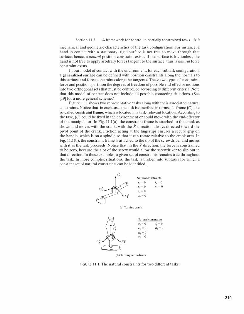
Section 11.3 A framework for control in partially constrained tasks 319
mechanical and geometric characteristics of the task configuration. For instance, ahand in contact with a stationary, rigid surface is not free to move through thatsurface; hence, a natural position constraint exists. If the surface is frictionless, thehand is not free to apply arbitrary forces tangent to the surface; thus, a natural forceconstraint exists.
In our model of contact with the environment, for each subtask configuration,a generalized surface can be defined with position constraints along the normals tothis surface and force constraints along the tangents. These two types of constraint,force and position, partition the degrees of freedom of possible end-effector motionsinto two orthogonal sets that must be controlled according to different criteria. Notethat this model of contact does not include all possible contacting situations. (See[19] for a more general scheme.)
Figure 11.1 shows two representative tasks along with their associated naturalconstraints. Notice that, in each case, the task is described in terms of a frame {C}, theso-called constraint frame, which is located in a task-relevant location. According tothe task, {C} could be fixed in the environment or could move with the end-effectorof the manipulator. In Fig. 11.1(a), the constraint frame is attached to the crank asshown and moves with the crank, with the X direction always directed toward thepivot point of the crank. Friction acting at the fingertips ensures a secure grip onthe handle, which is on a spindle so that it can rotate relative to the crank arm. InFig. 11.1(b), the constraint frame is attached to the tip of the screwdriver and moveswith it as the task proceeds. Notice that, in the Y direction, the force is constrainedto be zero, because the slot of the screw would allow the screwdriver to slip out inthat direction. In these examples, a given set of constraints remains true throughoutthe task. In more complex situations, the task is broken into subtasks for which aconstant set of natural constraints can be identified.
(a) Turning crank
(b) Turning screwdriver
CZ
CX
CX
CY
CY
Natural constraints
vx � 0 fy � 0
nz � 0
vz � 0
�x � 0
�y � 0
vx � 0
vz � 0
fy � 0
nz � 0
vx � 0
�y � 0
Natural constraints
CZ
FIGURE 11.1: The natural constraints for two different tasks.
319
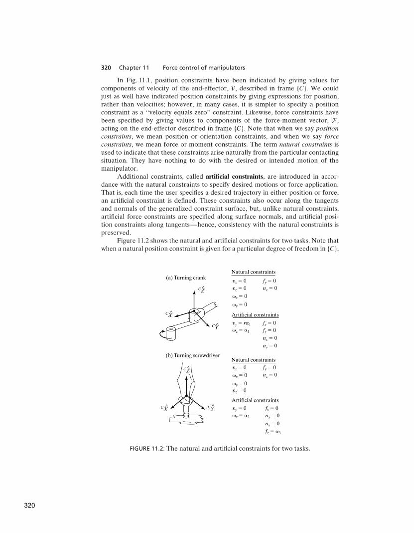
320 Chapter 11 Force control of manipulators
In Fig. 11.1, position constraints have been indicated by giving values forcomponents of velocity of the end-effector, V , described in frame {C}. We couldjust as well have indicated position constraints by giving expressions for position,rather than velocities; however, in many cases, it is simpler to specify a positionconstraint as a ‘‘velocity equals zero’’ constraint. Likewise, force constraints havebeen specified by giving values to components of the force-moment vector, F ,acting on the end-effector described in frame {C}. Note that when we say position
constraints, we mean position or orientation constraints, and when we say force
constraints, we mean force or moment constraints. The term natural constraints isused to indicate that these constraints arise naturally from the particular contactingsituation. They have nothing to do with the desired or intended motion of themanipulator.
Additional constraints, called artificial constraints, are introduced in accor-dance with the natural constraints to specify desired motions or force application.That is, each time the user specifies a desired trajectory in either position or force,an artificial constraint is defined. These constraints also occur along the tangentsand normals of the generalized constraint surface, but, unlike natural constraints,artificial force constraints are specified along surface normals, and artificial posi-tion constraints along tangents—hence, consistency with the natural constraints ispreserved.
Figure 11.2 shows the natural and artificial constraints for two tasks. Note thatwhen a natural position constraint is given for a particular degree of freedom in {C},
(a) Turning crank
(b) Turning screwdriver
CZ
CZ
CX
CX
CY
CY
Natural constraints
Artificial constraints
vx � 0
vy � 0
fy � 0
nz � 0
fx � 0
fz � �3
nx � 0
ny � 0
vz � 0
�x � 0
�z � �2
�y � 0
vx � 0
vz � 0
fy � 0
nz � 0
vy � r�1 fx � 0
fz � 0
nx � 0
ny � 0
�x � 0
�z � �1
�y � 0
Natural constraints
Artificial constraints
FIGURE 11.2: The natural and artificial constraints for two tasks.
320

Section 11.3 A framework for control in partially constrained tasks 321
an artificial force constraint should be specified, and vice versa. At any instant,any given degree of freedom in the constraint frame is controlled to meet either aposition or a force constraint.
Assembly strategy is a term that refers to a sequence of planned artificialconstraints that will cause the task to proceed in a desirable manner. Such strategiesmust include methods by which the system can detect a change in the contactingsituation so that transitions in the natural constraints can be tracked. With eachsuch change in natural constraints, a new set of artificial constraints is recalledfrom the set of assembly strategies and enforced by the control system. Methodsfor automatically choosing the constraints for a given assembly task await furtherresearch. In this chapter, we will assume that a task has been analyzed in orderto determine the natural constraints and that a human planner has determined anassembly strategy with which to control the manipulator.
Note that we will usually ignore friction forces between contacting surfaces inour analysis of tasks. This will suffice for our introduction to the problem and in factwill yield strategies that work in many cases. Usually friction forces of sliding areacting in directions chosen to be position controlled, and so these forces appear asdisturbances to the position servo and are overcome by the control system.
EXAMPLE 11.1
Figure 11.3(a)–(d) shows an assembly sequence used to put a round peg into a roundhole. The peg is brought down onto the surface to the left of the hole and then slidalong the surface until it drops into the hole. It is then inserted until the peg reachesthe bottom of the hole, at which time the assembly is complete. Each of the fourindicated contacting situations defines a subtask. For each of the subtasks shown,give the natural and artificial constraints. Also, indicate how the system senses thechange in the natural constraints as the operation proceeds.
First, we will attach the constraint frame to the peg as shown in Fig. 11.3(a). InFig. 11.3(a), the peg is in free space, and so the natural constraints are
CF = 0. (11.1)
(b)(a) (c) (d)
CX
CZ
FIGURE 11.3: The sequence of four contacting situations for peg insertion.
321

322 Chapter 11 Force control of manipulators
Therefore, the artificial constraints in this case constitute an entire position trajec-tory, which moves the peg in the CZ direction toward the surface. For example,
Cν =
00
υapproach
000
, (11.2)
where υapproach is the speed with which to approach the surface.
In Fig. 11.3(b), the peg has reached the surface. To detect that this hashappened, we observe the force in the CZ direction. When this sensed force exceedsa threshold, we sense contact, which implies a new contacting situation with a newset of natural constraints. Assuming that the contacting situation is as shown inFig. 11.3(b), the peg is not free to move in CZ, or to rotate about CX or C Y . Inthe other three degrees of freedom, it is not free to apply forces; hence, the naturalconstraints are
Cυz = 0,
Cωx = 0,
Cωy = 0, (11.3)
Cfx = 0,
Cfy = 0,
Cnz = 0.
The artificial constraints describe the strategy of sliding along the surface in the CX
direction while applying small forces to ensure that contact is maintained. Thus, wehave
Cυx = υslide,
Cυy = 0,
Cωz = 0,
Cfz = fcontact, (11.4)
Cnx = 0,
Cny = 0.
where fcontact is the force applied normal to the surface as the peg is slid, and υslideis the velocity with which to slide across the surface.
In Fig. 11.3(c), the peg has fallen slightly into the hole. This situation is sensedby observing the velocity in the CZ direction and waiting for it to cross a threshold(to become nonzero, in the ideal case). When this is observed, it signals that onceagain the natural constraints have changed, and thus our strategy (as embodied in
322
Section 11.4 The hybrid position/force control problem 323
the artificial constraints) must change. The new natural constraints are
Cυx = 0,
Cυy = 0,
Cωx = 0,
Cωy = 0, (11.5)
Cfx = 0,
Cnz = 0.
We choose the artificial constraints to be
Cυz = υinsert,
Cωz = 0,
Cfx = 0, (11.6)
Cfy = 0,
Cnx = 0,
Cny = 0,
where υinsert is the velocity at which the peg is inserted into the hole. Finally,
the situation shown in Fig. 11.3(d) is detected when the force in the CZ directionincreases above a threshold.
It is interesting to note that changes in the natural constraints are alwaysdetected by observing the position or force variable that is not being controlled. Forexample, to detect the transition from Fig. 11.3(b) to Fig. 11.3(c), we monitor thevelocity in CZ while we are controlling force in CZ. To discover when the peg hashit the bottom of the hole, we monitor Cfz, although we are controlling Cυz.
The framework we have introduced is somewhat simplistic. A more general andrigorous method of ‘‘splitting’’ tasks into position-controlled and force-controlledcomponents can be found in [19].
Determining assembly strategies for fitting more complicated parts togetheris quite complex. We have also neglected the effects of uncertainty in our simpleanalysis of this task. The development of automatic planning systems that includethe effects of uncertainty and can be applied to practical situations has been aresearch topic [4–8]. For a good review of these methods, see [9].
11.4 THE HYBRID POSITION/FORCE CONTROL PROBLEM
Figure 11.4 shows two extreme examples of contacting situations. In Fig. 11.4(a), themanipulator is moving through free space. In this case, the natural constraints areall force constraints—there is nothing to react against, so all forces are constrained
323
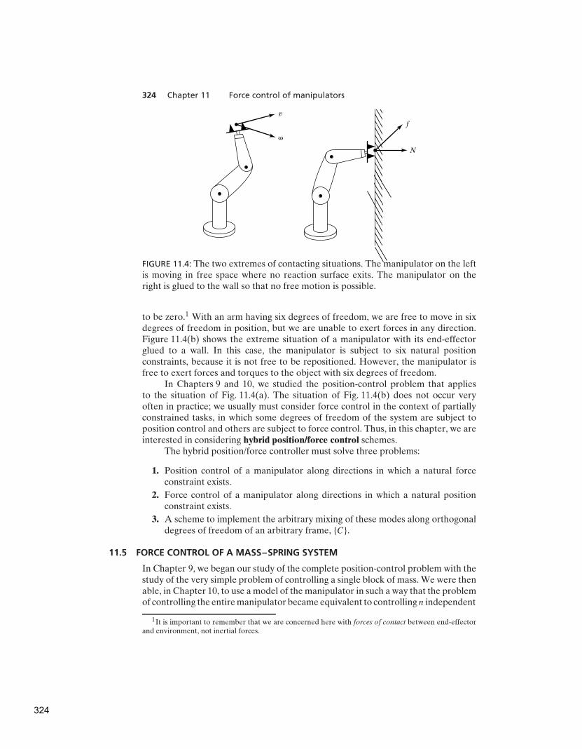
324 Chapter 11 Force control of manipulators
v
�
f
N
FIGURE 11.4: The two extremes of contacting situations. The manipulator on the leftis moving in free space where no reaction surface exits. The manipulator on theright is glued to the wall so that no free motion is possible.
to be zero.1 With an arm having six degrees of freedom, we are free to move in sixdegrees of freedom in position, but we are unable to exert forces in any direction.Figure 11.4(b) shows the extreme situation of a manipulator with its end-effectorglued to a wall. In this case, the manipulator is subject to six natural positionconstraints, because it is not free to be repositioned. However, the manipulator isfree to exert forces and torques to the object with six degrees of freedom.
In Chapters 9 and 10, we studied the position-control problem that appliesto the situation of Fig. 11.4(a). The situation of Fig. 11.4(b) does not occur veryoften in practice; we usually must consider force control in the context of partiallyconstrained tasks, in which some degrees of freedom of the system are subject toposition control and others are subject to force control. Thus, in this chapter, we areinterested in considering hybrid position/force control schemes.
The hybrid position/force controller must solve three problems:
1. Position control of a manipulator along directions in which a natural forceconstraint exists.
2. Force control of a manipulator along directions in which a natural positionconstraint exists.
3. A scheme to implement the arbitrary mixing of these modes along orthogonaldegrees of freedom of an arbitrary frame, {C}.
11.5 FORCE CONTROL OF A MASS–SPRING SYSTEM
In Chapter 9, we began our study of the complete position-control problem with thestudy of the very simple problem of controlling a single block of mass. We were thenable, in Chapter 10, to use a model of the manipulator in such a way that the problemof controlling the entire manipulator became equivalent to controlling n independent
1It is important to remember that we are concerned here with forces of contact between end-effectorand environment, not inertial forces.
324
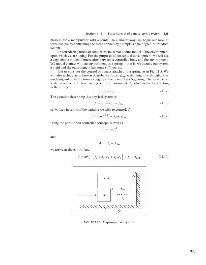
Section 11.5 Force control of a mass–spring system 325
masses (for a manipulator with n joints). In a similar way, we begin our look atforce control by controlling the force applied by a simple single-degree-of-freedomsystem.
In considering forces of contact, we must make some model of the environmentupon which we are acting. For the purposes of conceptual development, we will usea very simple model of interaction between a controlled body and the environment.We model contact with an environment as a spring—that is, we assume our systemis rigid and the environment has some stiffness, ke.
Let us consider the control of a mass attached to a spring, as in Fig. 11.5. Wewill also include an unknown disturbance force, fdist, which might be thought of asmodeling unknown friction or cogging in the manipulator’s gearing. The variable wewish to control is the force acting on the environment, fe, which is the force actingin the spring:
fe = kex. (11.7)
The equation describing this physical system is
f = mx + kex + fdist, (11.8)
or, written in terms of the variable we wish to control, fe,
f = mk−1efe + fe + fdist. (11.9)
Using the partitioned-controller concept, as well as
α = mk−1e
and
β = fe + fdist
we arrive at the control law,
f = mk−1e
[
fd + kυf ef + kpf ef
]
+ fe + fdist, (11.10)
x
m
ke
fdist
f
FIGURE 11.5: A spring–mass system.
325

326 Chapter 11 Force control of manipulators
where ef = fd − fe is the force error between the desired force, fd , and the sensedforce on the environment, fe. If we could compute (11.10), we would have theclosed-loop system
ef + kυf ef + kpf ef = 0. (11.11)
However, we cannot use knowledge of fdist in our control law, and so (11.10)is not feasible. We might leave that term out of the control law, but a steady-stateanalysis shows that there is a better choice, especially when the stiffness of theenvironment, ke, is high (the usual situation).
If we choose to leave the fdist term out of our control law, equate (11.9) and(11.10), and do a steady-state analysis by setting all time derivatives to zero, wefind that
ef =fdist
α, (11.12)
where α = mk−1ekpf , the effective force-feedback gain; however, if we choose to use
fd in the control law (11.10) in place of the term fe + fdist, we find the steady-stateerror to be
ef =fdist
1 + α. (11.13)
When the environment is stiff, as is often the case, α might be small, and so thesteady-state error calculated in (11.13) is quite an improvement over that of (11.12).Therefore, we suggest the control law
f = mk−1e
[
fd + kυf ef + kpf ef
]
+ fd . (11.14)
Figure 11.6 is a block diagram of the closed-loop system using the control law (11.14).Generally, practical considerations change the implementation of a force-
control servo quite a bit from the ideal shown in Fig. 11.6. First, force trajectories are
�
�
�
�
�
�
�
�
�
�
��
�
KpfKyf
mke�1fD
..
fD
.
fD
f � mx � kex � fdist.. fef
System
ddt
FIGURE 11.6: A force control system for the spring–mass system.
326

Section 11.5 Force control of a mass–spring system 327
��
�
�
� �
��
�
m
kyf
fDf � mx � kex � fdist
..
fe
fe
f
System
kpf
ke
x.
x.
FIGURE 11.7: A practical force-control system for the spring–mass system.
usually constants—that is, we are usually interested in controlling the contact forceto be at some constant level. Applications in which contact forces should followsome arbitrary function of time are rare. Therefore, the fd and fd inputs of thecontrol system are very often permanently set to zero. Another reality is that sensedforces are quite ‘‘noisy,’’ and numerical differentiation to compute fe is ill-advised.However, fe = kex, so we can obtain the derivative of the force on the environmentas fe = kex. This is much more realistic, in that most manipulators have means ofobtaining good measures of velocity. Having made these two pragmatic choices, wewrite the control law as
f = m[
kpf k−1eef − kυf x
]
+ fd , (11.15)
with the corresponding block diagram shown in Fig. 11.7.Note that an interpretation of the system of Fig. 11.7 is that force errors
generate a set-point for an inner velocity-control loop with gain kυf . Some force-control laws also include an integral term to improve steady-state performance.
An important remaining problem is that the stiffness of the environment, ke,appears in our control law, but is often unknown and perhaps changes from time totime. However, often an assembly robot is dealing with rigid parts, and ke could beguessed to be quite high. Generally this assumption is made, and gains are chosensuch that the system is somewhat robust with respect to variations in ke.
The purpose in constructing a control law to control the force of contact hasbeen to show one suggested structure and to expose a few issues. For the remainderof this chapter, we will simply assume that such a force-controlling servo could bebuilt and abstract it away into a black box, as shown in Fig. 11.8. In practice, it is noteasy to build a high-performance force servo, and it is currently an area of activeresearch [11–14]. For a good review of this area, see [15].
327
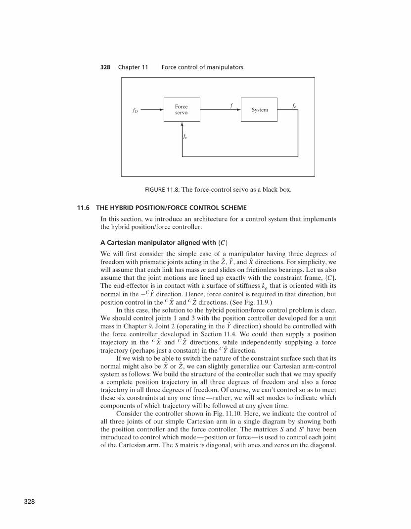
328 Chapter 11 Force control of manipulators
Forceservo
SystemfD
fe
fef
FIGURE 11.8: The force-control servo as a black box.
11.6 THE HYBRID POSITION/FORCE CONTROL SCHEME
In this section, we introduce an architecture for a control system that implementsthe hybrid position/force controller.
A Cartesian manipulator aligned with {C}
We will first consider the simple case of a manipulator having three degrees offreedom with prismatic joints acting in the Z, Y , and X directions. For simplicity, wewill assume that each link has mass m and slides on frictionless bearings. Let us alsoassume that the joint motions are lined up exactly with the constraint frame, {C}.The end-effector is in contact with a surface of stiffness ke that is oriented with its
normal in the −C Y direction. Hence, force control is required in that direction, butposition control in the CX and CZ directions. (See Fig. 11.9.)
In this case, the solution to the hybrid position/force control problem is clear.We should control joints 1 and 3 with the position controller developed for a unitmass in Chapter 9. Joint 2 (operating in the Y direction) should be controlled withthe force controller developed in Section 11.4. We could then supply a positiontrajectory in the CX and CZ directions, while independently supplying a forcetrajectory (perhaps just a constant) in the C Y direction.
If we wish to be able to switch the nature of the constraint surface such that itsnormal might also be X or Z, we can slightly generalize our Cartesian arm-controlsystem as follows: We build the structure of the controller such that we may specifya complete position trajectory in all three degrees of freedom and also a forcetrajectory in all three degrees of freedom. Of course, we can’t control so as to meetthese six constraints at any one time—rather, we will set modes to indicate whichcomponents of which trajectory will be followed at any given time.
Consider the controller shown in Fig. 11.10. Here, we indicate the control ofall three joints of our simple Cartesian arm in a single diagram by showing boththe position controller and the force controller. The matrices S and S′ have beenintroduced to control which mode—position or force—is used to control each jointof the Cartesian arm. The S matrix is diagonal, with ones and zeros on the diagonal.
328
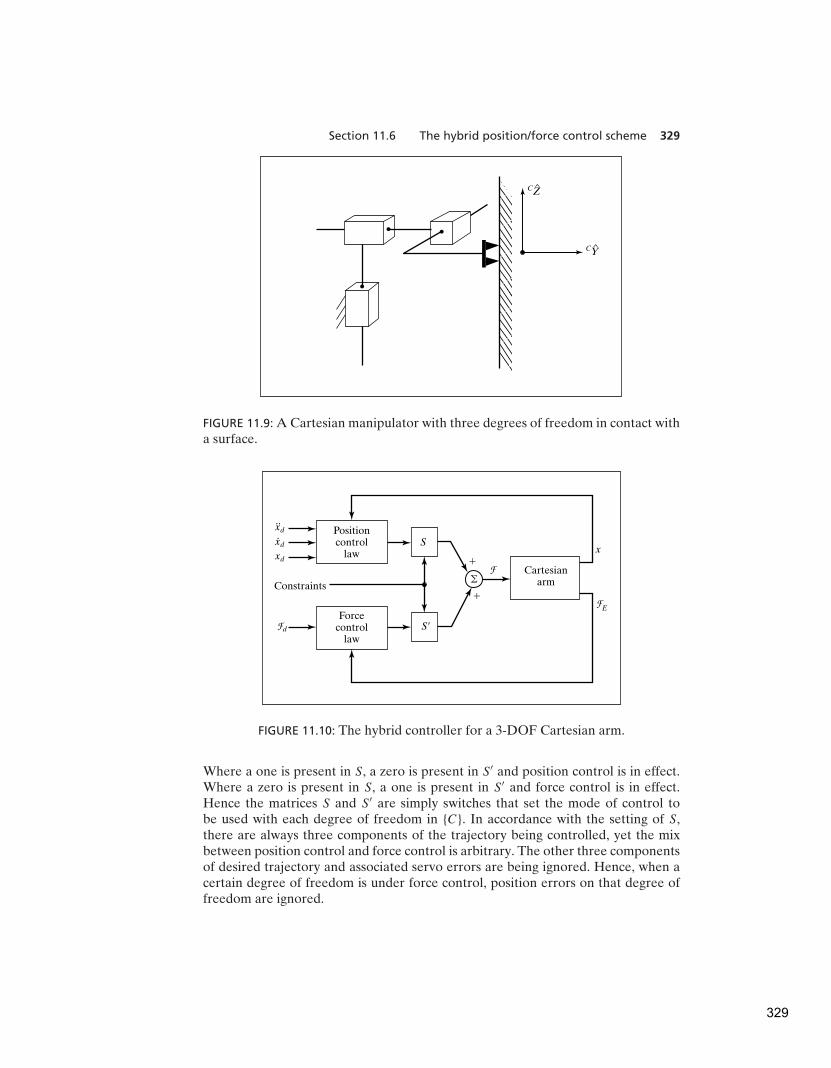
Section 11.6 The hybrid position/force control scheme 329
CZ
CY
FIGURE 11.9: A Cartesian manipulator with three degrees of freedom in contact witha surface.
�
�
�Cartesian
arm
S
S�
Forcecontrol
law
Positioncontrol
lawxd
xxd.xd..
Constraints
E
d
FIGURE 11.10: The hybrid controller for a 3-DOF Cartesian arm.
Where a one is present in S, a zero is present in S′ and position control is in effect.Where a zero is present in S, a one is present in S′ and force control is in effect.Hence the matrices S and S′ are simply switches that set the mode of control tobe used with each degree of freedom in {C}. In accordance with the setting of S,there are always three components of the trajectory being controlled, yet the mixbetween position control and force control is arbitrary. The other three componentsof desired trajectory and associated servo errors are being ignored. Hence, when acertain degree of freedom is under force control, position errors on that degree offreedom are ignored.
329

330 Chapter 11 Force control of manipulators
EXAMPLE 11.2
For the situation shown in Fig. 11.9, with motions in the C Y direction constrainedby the reaction surface, give the matrices S and S′.
Because the X and Z components are to be position controlled, we enter oneson the diagonal of S corresponding to these two components. This will cause theposition servo to be active in these two directions, and the input trajectory will befollowed. Any position trajectory input for the Y component will be ignored. The S′
matrix has the ones and zeros on the diagonal inverted; hence, we have
S =
1 0 00 0 00 0 1
,
S′ =
0 0 00 1 00 0 0
. (11.16)
Figure 11.10 shows the hybrid controller for the special case that the jointsline up exactly with the constraint frame, {C}. In the following subsection, we usetechniques studied in previous chapters to generalize the controller to work withgeneral manipulators and for an arbitrary {C}; however, in the ideal case, the systemperforms as if the manipulator had an actuator ‘‘lined up’’ with each of the degreesof freedom in {C}.
A general manipulator
Generalizing the hybrid controller shown in Fig. 11.10 so that a general manipulatormay be used is straightforward with the concept of Cartesian-based control. Chapter6 discussed how the equations of motion of a manipulator could be written interms of Cartesian motion of the end-effector, and Chapter 10 showed how sucha formulation might be used to achieve decoupled Cartesian position control of amanipulator. The major idea is that, through use of a dynamic model written inCartesian space, it is possible to control so that the combined system of the actualmanipulator and computed model appear as a set of independent, uncoupled unitmasses. Once this decoupling and linearizing are done, we can apply the simpleservo already developed in Section 11.4.
Figure 11.11 shows the compensation based on the formulation of the manip-ulator dynamics in Cartesian space such that the manipulator appears as a set ofuncoupled unit masses. For use in the hybrid control scheme, the Cartesian dynamicsand the Jacobian are written in the constraint frame, {C}. Likewise, the kinematicsare computed with respect to the constraint frame.
Because we have designed the hybrid controller for a Cartesian manipulatoraligned with the constraint frame, and because the Cartesian decoupling schemeprovides us with a system with the same input–output properties, we need onlycombine the two to generate the generalized hybrid position/force controller.
Figure 11.12 is a block diagram of the hybrid controller for a general manipu-lator. Note that the dynamics are written in the constraint frame, as is the Jacobian.
330
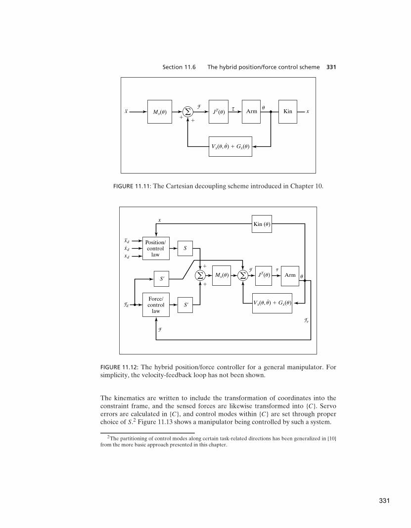
Section 11.6 The hybrid position/force control scheme 331
��
au
x..
xMx(u) JT(u) Arm Kin
Vx(u, u) � Gx(u).
t
FIGURE 11.11: The Cartesian decoupling scheme introduced in Chapter 10.
�
�
u
t
xd..
xd.
xd
x
Mx(u) JT(u) Arm
Kin (u)
Vx(u, u) � Gx(u).
e
d
Position/control
law
Force/control
law
S
S�
S� a a
FIGURE 11.12: The hybrid position/force controller for a general manipulator. Forsimplicity, the velocity-feedback loop has not been shown.
The kinematics are written to include the transformation of coordinates into theconstraint frame, and the sensed forces are likewise transformed into {C}. Servoerrors are calculated in {C}, and control modes within {C} are set through properchoice of S.2 Figure 11.13 shows a manipulator being controlled by such a system.
2The partitioning of control modes along certain task-related directions has been generalized in [10]
from the more basic approach presented in this chapter.
331
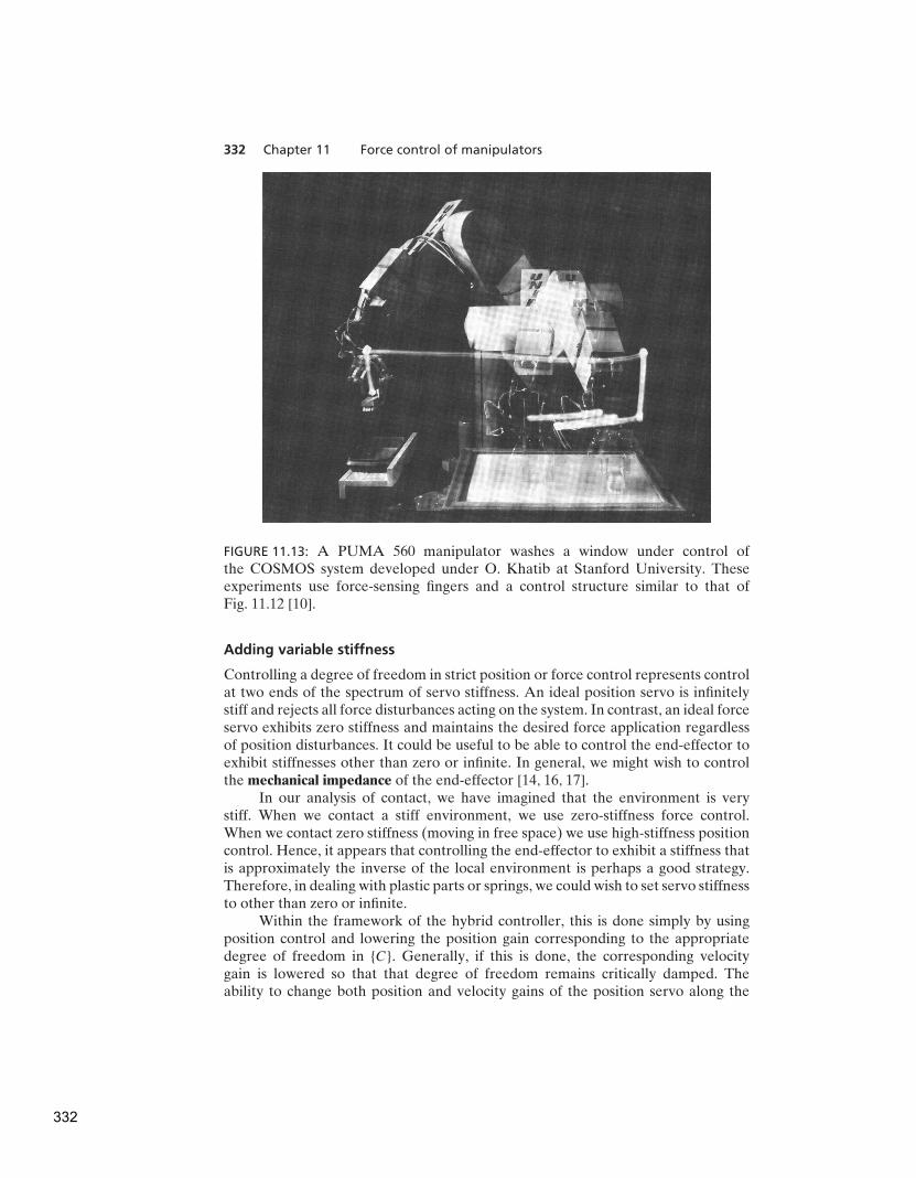
332 Chapter 11 Force control of manipulators
FIGURE 11.13: A PUMA 560 manipulator washes a window under control ofthe COSMOS system developed under O. Khatib at Stanford University. Theseexperiments use force-sensing fingers and a control structure similar to that ofFig. 11.12 [10].
Adding variable stiffness
Controlling a degree of freedom in strict position or force control represents controlat two ends of the spectrum of servo stiffness. An ideal position servo is infinitelystiff and rejects all force disturbances acting on the system. In contrast, an ideal forceservo exhibits zero stiffness and maintains the desired force application regardlessof position disturbances. It could be useful to be able to control the end-effector toexhibit stiffnesses other than zero or infinite. In general, we might wish to controlthe mechanical impedance of the end-effector [14, 16, 17].
In our analysis of contact, we have imagined that the environment is verystiff. When we contact a stiff environment, we use zero-stiffness force control.When we contact zero stiffness (moving in free space) we use high-stiffness positioncontrol. Hence, it appears that controlling the end-effector to exhibit a stiffness thatis approximately the inverse of the local environment is perhaps a good strategy.Therefore, in dealing with plastic parts or springs, we could wish to set servo stiffnessto other than zero or infinite.
Within the framework of the hybrid controller, this is done simply by usingposition control and lowering the position gain corresponding to the appropriatedegree of freedom in {C}. Generally, if this is done, the corresponding velocitygain is lowered so that that degree of freedom remains critically damped. Theability to change both position and velocity gains of the position servo along the
332

Section 11.7 Current industrial-robot control schemes 333
degrees of freedom of {C} allows the hybrid position/force controller to implementa generalized impedance of the end-effector [17]. However, in many practicalsituations we are dealing with the interaction of stiff parts, so that pure positioncontrol or pure force control is desired.
11.7 CURRENT INDUSTRIAL-ROBOT CONTROL SCHEMES
True force control, such as the hybrid position/force controller introduced in thischapter, does not exist today in industrial robots. Among the problems of practicalimplementation are the rather large amount of computation required, lack ofaccurate parameters for the dynamic model, lack of rugged force sensors, and theburden of difficulty placed on the user in specifying a position/force strategy.
Passive compliance
Extremely rigid manipulators with very stiff position servos are ill-suited to tasks inwhich parts come into contact and contact forces are generated. In such situations,parts are often jammed or damaged. Ever since early experiments with manipulatorsattempting to do assembly, it was realized that, to the extent that the robots couldperform such tasks, it was only thanks to the compliance of the parts, of the fixtures,or of the arm itself. This ability of one or more parts of the system to ‘‘give’’ a littlewas often enough to allow the successful mating of parts.
Once this was realized, devices were specially designed to introduce complianceinto the system on purpose. The most successful such device is the RCC or remote
center compliance device developed at Draper Labs [18]. The RCC was cleverlydesigned so that it introduced the ‘‘right’’ kind of compliance, which allowed certaintasks to proceed smoothly and rapidly with little or no chance of jamming. TheRCC is essentially a spring with six degrees of freedom, which is inserted betweenthe manipulator’s wrist and the end-effector. By setting the stiffnesses of the sixsprings, various amounts of compliance can be introduced. Such schemes are calledpassive-compliance schemes and are used in industrial applications of manipulatorsin some tasks.
Compliance through softening position gains
Rather than achieving compliance in a passive, and therefore fixed, way, it ispossible to devise schemes in which the apparent stiffness of the manipulatoris altered through adjustment of the gains of a position-control system. A fewindustrial robots do something of this type for applications such as grinding, inwhich contact with a surface needs to be maintained but delicate force control is notrequired.
A particularly interesting approach has been suggested by Salisbury [16]. Inthis scheme, the position gains in a joint-based servo system are modified in such away that the end-effector appears to have a certain stiffness along Cartesian degreesof freedom: Consider a general spring with six degrees of freedom. Its action couldbe described by
F = Kpxδχ, (11.17)
333

334 Chapter 11 Force control of manipulators
where Kpx is a diagonal 6 × 6 matrix with three linear stiffnesses followed by threetorsional stiffnesses on the diagonal. How could we make the end-effector of amanipulator exhibit this stiffness characteristic?
Recalling the definition of the manipulator Jacobian, we have
δχ = J (�)δ�. (11.18)
Combining with (11.17) gives
F = KpxJ (�)δ�. (11.19)
From static-force considerations, we have
τ = J T (�)F, (11.20)
which, combined with (11.19), yields
τ = J T (�)KpxJ (�)δ�. (11.21)
Here, the Jacobian is usually written in the tool frame. Equation (11.21) is anexpression for how joint torques should be generated as a function of small changesin joint angles, δ�, in order to make the manipulator end-effector behave as aCartesian spring with six degrees of freedom.
Whereas a simple joint-based position controller might use the control law
τ = KpE +KυE, (11.22)
where Kp and Kυ are constant diagonal gain matrices and E is servo error definedas �d −�, Salisbury suggests using
τ = J T (�)KpxJ (�)E +KυE, (11.23)
where Kpx is the desired stiffness of the end-effector in Cartesian space. For amanipulator with six degrees of freedom, Kpx is diagonal with the six values on thediagonal representing the three translational and three rotational stiffnesses thatthe end-effector is to exhibit. Essentially, through use of the Jacobian, a Cartesianstiffness has been transformed to a joint-space stiffness.
Force sensing
Force sensing allows a manipulator to detect contact with a surface and, using thissensation, to take some action. For example, the term guarded move is sometimesused to mean the strategy of moving under position control until a force is felt,then halting motion. Additionally, force sensing can be used to weigh objects thatthe manipulator lifts. This can be used as a simple check during a parts-handlingoperation—to ensure that a part was acquired or that the appropriate part wasacquired.
Some commercially available robots come equipped with force sensors in theend-effector. These robots can be programmed to stop motion or take other action
334

Bibliography 335
when a force threshold is exceeded, and some can be programmed to weigh objectsthat are grasped in the end-effector.
BIBLIOGRAPHY
[1] M. Mason, ‘‘Compliance and Force Control for Computer Controlled Manipulators,’’M.S. Thesis, MIT AI Laboratory, May 1978.
[2] J. Craig and M. Raibert, ‘‘A Systematic Method for Hybrid Position/Force Controlof a Manipulator,’’ Proceedings of the 1979 IEEE Computer Software Applications
Conference, Chicago, November 1979.
[3] M. Raibert and J. Craig, ‘‘Hybrid Position/Force Control of Manipulators,’’ ASME
Journal of Dynamic Systems, Measurement, and Control, June 1981.
[4] T. Lozano-Perez, M. Mason, and R. Taylor, ‘‘Automatic Synthesis of Fine-MotionStrategies for Robots,’’ 1st International Symposium of Robotics Research, BrettonWoods, NH, August 1983.
[5] M. Mason, ‘‘Automatic Planning of Fine Motions: Correctness and Completeness,’’IEEE International Conference on Robotics, Atlanta, March 1984.
[6] M. Erdmann, ‘‘Using Backprojections for the Fine Motion Planning with Uncer-tainty,’’ The International Journal of Robotics Research, Vol. 5, No. 1, 1986.
[7] S. Buckley, ‘‘Planning and Teaching Compliant Motion Strategies,’’ Ph.D. Disserta-tion, Department of Electrical Engineering and Computer Science, MIT, January1986.
[8] B. Donald, ‘‘Error Detection and Recovery for Robot Motion Planning with Uncer-tainty,’’ Ph.D. Dissertation, Department of Electrical Engineering and ComputerScience, MIT, July 1987.
[9] J.C. Latombe, ‘‘Motion Planning with Uncertainty: On the Preimage Backchain-ing Approach,’’ in The Robotics Review, O. Khatib, J. Craig, and T. Lozano-Perez,Editors, MIT Press, Cambridge, MA, 1988.
[10] O. Khatib, ‘‘A Unified Approach for Motion and Force Control of Robot Manipula-tors: The Operational Space Formulation,’’ IEEE Journal of Robotics and Automation,Vol. RA-3, No. 1, 1987.
[11] D. Whitney, ‘‘Force Feedback Control of Manipulator Fine Motions,’’ ProceedingsJoint Automatic Control Conference, San Francisco, 1976.
[12] S. Eppinger and W. Seering, ‘‘Understanding Bandwidth Limitations in Robot ForceControl,’’ Proceedings of the IEEE Conference on Robotics and Automation, Raleigh,NC, 1987.
[13] W. Townsend and J.K. Salisbury, ‘‘The Effect of Coulomb Friction and Stiction onForce Control,’’ Proceedings of the IEEE Conference on Robotics and Automation,Raleigh, NC, 1987.
[14] N. Hogan, ‘‘Stable Execution of Contact Tasks Using Impedance Control,’’ Proceed-
ings of the IEEE Conference on Robotics and Automation, Raleigh, NC, 1987.
[15] N. Hogan and E. Colgate, ‘‘Stability Problems in Contact Tasks,’’ in The Robotics
Review, O. Khatib, J. Craig, and T. Lozano-Perez, Editors, MIT Press, Cambridge,MA, 1988.
[16] J.K. Salisbury, ‘‘Active Stiffness Control of a Manipulator in Cartesian Coordinates,’’19th IEEE Conference on Decision and Control, December 1980.
335

336 Chapter 11 Force control of manipulators
[17] J.K. Salisbury and J. Craig, ‘‘Articulated Hands: Force Control and Kinematic Issues,’’International Journal of Robotics Research, Vol. 1, No. 1.
[18] S. Drake, ‘‘Using Compliance in Lieu of Sensory Feedback for Automatic Assembly,’’Ph.D. Thesis, Mechanical Engineering Department, MIT, September 1977.
[19] R. Featherstone, S.S. Thiebaut, and O. Khatib, ‘‘A General Contact Model forDynamically-Decoupled Force/Motion Control,’’ Proceedings of the IEEE Conference
on Robotics and Automation, Detroit, 1999.
EXERCISES
11.1 [12] Give the natural constraints present for a peg of square cross section slidinginto a hole of square cross section. Show your definition of {C} in a sketch.
11.2 [10] Give the artificial constraints (i.e., the trajectory) you would suggest in orderto cause the peg in Exercise 11.1 to slide further into the hole without jamming.
11.3 [20] Show that using the control law (11.14) with a system given by (11.9) resultsin the error-space equation
ef + kυfef + (kpf +m−1ke)ef = m−1kefdist,
and, hence, that choosing gains to provide critical damping is possible only if thestiffness of the environment, ke, is known.
11.4 [17] Given
A
BT =
0.866 −0.500 0.000 10.00.500 0.866 0.000 0.00.000 0.000 1.000 5.0
0 0 0 1
,
if the force–torque vector at the origin of {A} is
Aν =
0.02.0
−3.00.00.04.0
,
find the 6 × 1 force–torque vector with reference point at the origin of {B}.11.5 [17] Given
A
BT =
0.866 0.500 0.000 10.0−0.500 0.866 0.000 0.0
0.000 0.000 1.000 5.00 0 0 1
,
if the force–torque vector at the origin of {A} is
Aν =
6.06.00.05.00.00.0
,
find the 6 × 1 force–torque vector with reference point at the origin of {B}.
336
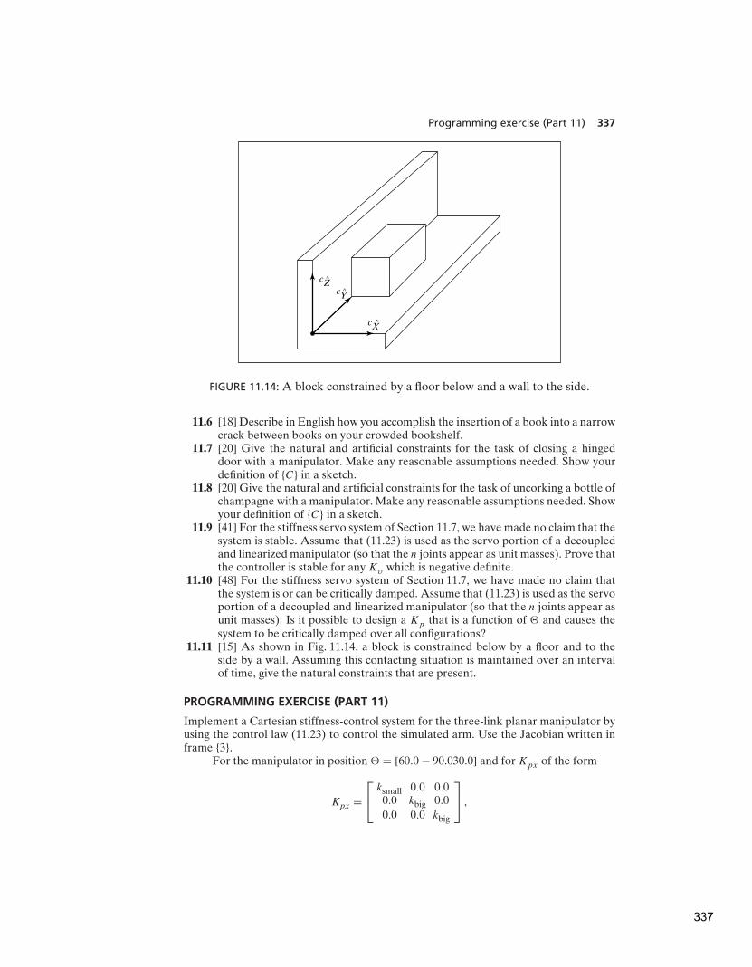
Programming exercise (Part 11) 337
cY^
cX^
cZ^
FIGURE 11.14: A block constrained by a floor below and a wall to the side.
11.6 [18] Describe in English how you accomplish the insertion of a book into a narrowcrack between books on your crowded bookshelf.
11.7 [20] Give the natural and artificial constraints for the task of closing a hingeddoor with a manipulator. Make any reasonable assumptions needed. Show yourdefinition of {C} in a sketch.
11.8 [20] Give the natural and artificial constraints for the task of uncorking a bottle ofchampagne with a manipulator. Make any reasonable assumptions needed. Showyour definition of {C} in a sketch.
11.9 [41] For the stiffness servo system of Section 11.7, we have made no claim that thesystem is stable. Assume that (11.23) is used as the servo portion of a decoupledand linearized manipulator (so that the n joints appear as unit masses). Prove thatthe controller is stable for any Kυ which is negative definite.
11.10 [48] For the stiffness servo system of Section 11.7, we have made no claim thatthe system is or can be critically damped. Assume that (11.23) is used as the servoportion of a decoupled and linearized manipulator (so that the n joints appear asunit masses). Is it possible to design a Kp that is a function of � and causes thesystem to be critically damped over all configurations?
11.11 [15] As shown in Fig. 11.14, a block is constrained below by a floor and to theside by a wall. Assuming this contacting situation is maintained over an intervalof time, give the natural constraints that are present.
PROGRAMMING EXERCISE (PART 11)
Implement a Cartesian stiffness-control system for the three-link planar manipulator byusing the control law (11.23) to control the simulated arm. Use the Jacobian written inframe {3}.
For the manipulator in position � = [60.0 − 90.030.0] and for Kpx of the form
Kpx =
ksmall 0.0 0.00.0 kbig 0.0
0.0 0.0 kbig
,
337
338 Chapter 11 Force control of manipulators
simulate the application of the following static forces:
1. a 1-newton force acting at the origin of {3} in the X3 direction, and
2. a 1-newton force acting at the origin of {3} in the Y3 direction.
The values of ksmall and kbig should be found experimentally. Use a large value of
kbig for high stiffness in the Y3 direction and a low value of ksmall for low stiffness in the
X3 direction. What are the steady-state deflections in the two cases?
338
C H A P T E R 12
Robot programming languagesand systems
12.1 INTRODUCTION
12.2 THE THREE LEVELS OF ROBOT PROGRAMMING
12.3 A SAMPLE APPLICATION
12.4 REQUIREMENTS OF A ROBOT PROGRAMMING LANGUAGE
12.5 PROBLEMS PECULIAR TO ROBOT PROGRAMMING LANGUAGES
12.1 INTRODUCTION
In this chapter, we begin to consider the interface between the human user andan industrial robot. It is by means of this interface that a user takes advantage ofall the underlying mechanics and control algorithms we have studied in previouschapters.
The sophistication of the user interface is becoming extremely important asmanipulators and other programmable automation are applied to more and moredemanding industrial applications. It turns out that the nature of the user interfaceis a very important concern. In fact, most of the challenge of the design and use ofindustrial robots focuses on this aspect of the problem.
Robot manipulators differentiate themselves from fixed automation by being‘‘flexible,’’ which means programmable. Not only are the movements of manipulatorsprogrammable, but, through the use of sensors and communications with otherfactory automation, manipulators can adapt to variations as the task proceeds.
In considering the programming of manipulators, it is important to rememberthat they are typically only a minor part of an automated process. The termworkcell is used to describe a local collection of equipment, which may includeone or more manipulators, conveyor systems, parts feeders, and fixtures. At thenext higher level, workcells might be interconnected in factorywide networks sothat a central control computer can control the overall factory flow. Hence, theprogramming of manipulators is often considered within the broader problemof programming a variety of interconnected machines in an automated factoryworkcell.
Unlike that in the previous 11 chapters, the material in this chapter (and thenext chapter) is of a nature that constantly changes. It is therefore difficult to presentthis material in a detailed way. Rather, we attempt to point out the underlyingfundamental concepts, and we leave it to the reader to seek out the latest examples,as industrial technology continues to move forward.
From Chapter 12 of Introduction to Robotics: Mechanics and Control, Third Edition. John J. Craig.
Copyright © 2005 by Pearson Education, Inc. All rights reserved.
339
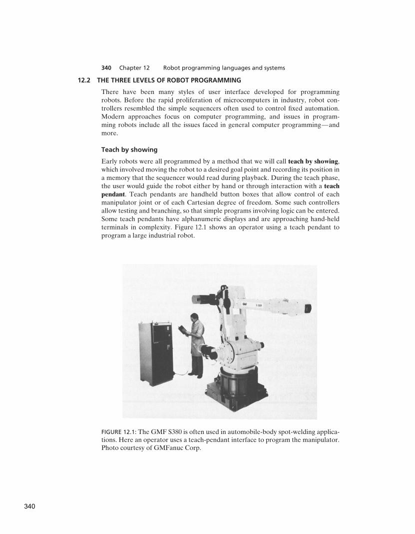
340 Chapter 12 Robot programming languages and systems
12.2 THE THREE LEVELS OF ROBOT PROGRAMMING
There have been many styles of user interface developed for programmingrobots. Before the rapid proliferation of microcomputers in industry, robot con-trollers resembled the simple sequencers often used to control fixed automation.Modern approaches focus on computer programming, and issues in program-ming robots include all the issues faced in general computer programming—andmore.
Teach by showing
Early robots were all programmed by a method that we will call teach by showing,which involved moving the robot to a desired goal point and recording its position ina memory that the sequencer would read during playback. During the teach phase,the user would guide the robot either by hand or through interaction with a teach
pendant. Teach pendants are handheld button boxes that allow control of eachmanipulator joint or of each Cartesian degree of freedom. Some such controllersallow testing and branching, so that simple programs involving logic can be entered.Some teach pendants have alphanumeric displays and are approaching hand-heldterminals in complexity. Figure 12.1 shows an operator using a teach pendant toprogram a large industrial robot.
FIGURE 12.1: The GMF S380 is often used in automobile-body spot-welding applica-tions. Here an operator uses a teach-pendant interface to program the manipulator.Photo courtesy of GMFanuc Corp.
340

Section 12.2 The three levels of robot programming 341
Explicit robot programming languages
Ever since the arrival of inexpensive and powerful computers, the trend hasbeen increasingly toward programming robots via programs written in computerprogramming languages. Usually, these computer programming languages havespecial features that apply to the problems of programming manipulators andso are called robot programming languages (RPLs). Most of the systems thatcome equipped with a robot programming language have nonetheless retained ateach-pendant-style interface also.
Robot programming languages have likewise taken on many forms. We willsplit them into three categories:
1. Specialized manipulation languages. These robot programming languages havebeen built by developing a completely new language that, although addressingrobot-specific areas, might well be considered a general computer program-ming language. An example is the VAL language developed to control theindustrial robots by Unimation, Inc [1]. VAL was developed especially as amanipulator control language; as a general computer language, it was quiteweak. For example, it did not support floating-point numbers or characterstrings, and subroutines could not pass arguments. A more recent version,V-II, provided these features [2]. The current incarnation of this language,V+, includes many new features [13]. Another example of a specialized manip-ulation language is AL, developed at Stanford University [3]. Although theAL language is now a relic of the past, it nonetheless provides good examplesof some features still not found in most modern languages (force control,parallelism). Also, because it was built in an academic environment, there arereferences available to describe it [3]. For these reasons, we continue to makereference to it.
2. Robot library for an existing computer language. These robot programminglanguages have been developed by starting with a popular computer lan-guage (e.g., Pascal) and adding a library of robot-specific subroutines. Theuser then writes a Pascal program making use of frequent calls to the prede-fined subroutine package for robot-specific needs. An examples is AR-BASICfrom American Cimflex [4], essentially a subroutine library for a standardBASIC implementation. JARS, developed by NASA’s Jet Propulsion Lab-oratory, is an example of such a robot programming language based onPascal [5].
3. Robot library for a new general-purpose language. These robot program-ming languages have been developed by first creating a new general-purposelanguage as a programming base and then supplying a library of predefinedrobot-specific subroutines. Examples of such robot programming languagesare RAPID developed by ABB Robotics [6], AML developed by IBM [7], andKAREL developed by GMF Robotics [8].
Studies of actual application programs for robotic workcells have shown thata large percentage of the language statements are not robot-specific [7]. Instead,a great deal of robot programming has to do with initialization, logic testing andbranching, communication, and so on. For this reason, a trend might develop to
341
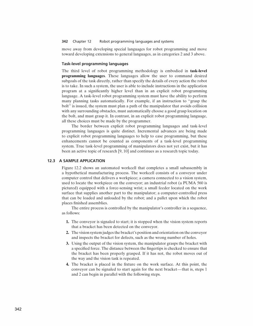
342 Chapter 12 Robot programming languages and systems
move away from developing special languages for robot programming and movetoward developing extensions to general languages, as in categories 2 and 3 above.
Task-level programming languages
The third level of robot programming methodology is embodied in task-level
programming languages. These languages allow the user to command desiredsubgoals of the task directly, rather than specify the details of every action the robotis to take. In such a system, the user is able to include instructions in the applicationprogram at a significantly higher level than in an explicit robot programminglanguage. A task-level robot programming system must have the ability to performmany planning tasks automatically. For example, if an instruction to ‘‘grasp thebolt’’ is issued, the system must plan a path of the manipulator that avoids collisionwith any surrounding obstacles, must automatically choose a good grasp location onthe bolt, and must grasp it. In contrast, in an explicit robot programming language,all these choices must be made by the programmer.
The border between explicit robot programming languages and task-levelprogramming languages is quite distinct. Incremental advances are being madeto explicit robot programming languages to help to ease programming, but theseenhancements cannot be counted as components of a task-level programmingsystem. True task-level programming of manipulators does not yet exist, but it hasbeen an active topic of research [9, 10] and continues as a research topic today.
12.3 A SAMPLE APPLICATION
Figure 12.2 shows an automated workcell that completes a small subassembly ina hypothetical manufacturing process. The workcell consists of a conveyor undercomputer control that delivers a workpiece; a camera connected to a vision system,used to locate the workpiece on the conveyor; an industrial robot (a PUMA 560 ispictured) equipped with a force-sensing wrist; a small feeder located on the worksurface that supplies another part to the manipulator; a computer-controlled pressthat can be loaded and unloaded by the robot; and a pallet upon which the robotplaces finished assemblies.
The entire process is controlled by the manipulator’s controller in a sequence,as follows:
1. The conveyor is signaled to start; it is stopped when the vision system reportsthat a bracket has been detected on the conveyor.
2. The vision system judges the bracket’s position and orientation on the conveyorand inspects the bracket for defects, such as the wrong number of holes.
3. Using the output of the vision system, the manipulator grasps the bracket witha specified force. The distance between the fingertips is checked to ensure thatthe bracket has been properly grasped. If it has not, the robot moves out ofthe way and the vision task is repeated.
4. The bracket is placed in the fixture on the work surface. At this point, theconveyor can be signaled to start again for the next bracket—that is, steps 1and 2 can begin in parallel with the following steps.
342

Section 12.3 A sample application 343
FIGURE 12.2: An automated workcell containing an industrial robot.
5. A pin is picked from the feeder and inserted partway into a tapered hole in thebracket. Force control is used to perform this insertion and to perform simplechecks on its completion. (If the pin feeder is empty, an operator is notifiedand the manipulator waits until commanded to resume by the operator.)
6. The bracket–pin assembly is grasped by the robot and placed in the press.
7. The press is commanded to actuate, and it presses the pin the rest of the wayinto the bracket. The press signals that it has completed, and the bracket isplaced back into the fixture for a final inspection.
8. By force sensing, the assembly is checked for proper insertion of the pin. Themanipulator senses the reaction force when it presses sideways on the pin andcan do several checks to discover how far the pin protrudes from the bracket.
9. If the assembly is judged to be good, the robot places the finished part into thenext available pallet location. If the pallet is full, the operator is signaled. Ifthe assembly is bad, it is dropped into the trash bin.
10. Once Step 2 (started earlier in parallel) is complete, go to Step 3.
This is an example of a task that is possible for today’s industrial robots. Itshould be clear that the definition of such a process through ‘‘teach by showing’’techniques is probably not feasible. For example, in dealing with pallets, it islaborious to have to teach all the pallet compartment locations; it is much preferableto teach only the corner location and then compute the others from knowledge ofthe dimensions of the pallet. Further, specifying interprocess signaling and settingup parallelism by using a typical teach pendant or a menu-style interface is usually
343
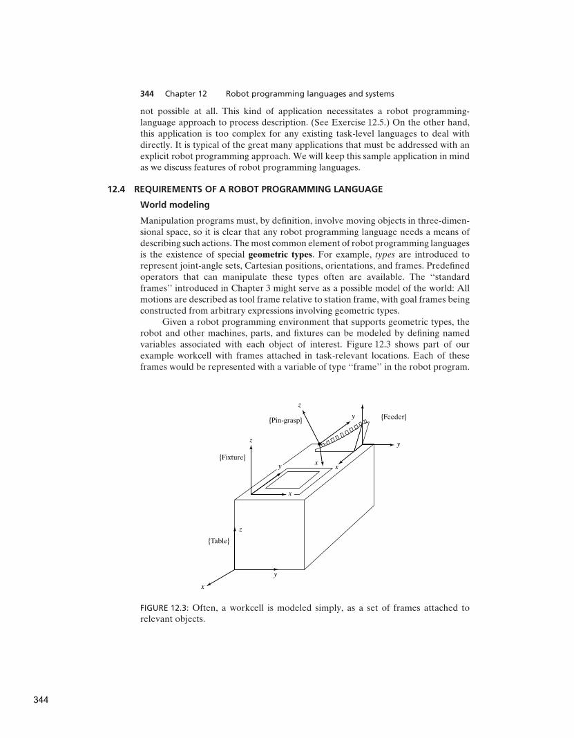
344 Chapter 12 Robot programming languages and systems
not possible at all. This kind of application necessitates a robot programming-language approach to process description. (See Exercise 12.5.) On the other hand,this application is too complex for any existing task-level languages to deal withdirectly. It is typical of the great many applications that must be addressed with anexplicit robot programming approach. We will keep this sample application in mindas we discuss features of robot programming languages.
12.4 REQUIREMENTS OF A ROBOT PROGRAMMING LANGUAGE
World modeling
Manipulation programs must, by definition, involve moving objects in three-dimen-sional space, so it is clear that any robot programming language needs a means ofdescribing such actions. The most common element of robot programming languagesis the existence of special geometric types. For example, types are introduced torepresent joint-angle sets, Cartesian positions, orientations, and frames. Predefinedoperators that can manipulate these types often are available. The ‘‘standardframes’’ introduced in Chapter 3 might serve as a possible model of the world: Allmotions are described as tool frame relative to station frame, with goal frames beingconstructed from arbitrary expressions involving geometric types.
Given a robot programming environment that supports geometric types, therobot and other machines, parts, and fixtures can be modeled by defining namedvariables associated with each object of interest. Figure 12.3 shows part of ourexample workcell with frames attached in task-relevant locations. Each of theseframes would be represented with a variable of type ‘‘frame’’ in the robot program.
z
y
yz
z
y
x
xx
{Table}
{Fixture}
{Pin-grasp}{Feeder}
y
x
FIGURE 12.3: Often, a workcell is modeled simply, as a set of frames attached torelevant objects.
344

Section 12.4 Requirements of a robot programming language 345
In many robot programming languages, this ability to define named variablesof various geometric types and refer to them in the program forms the basis of theworld model. Note that the physical shapes of the objects are not part of such a worldmodel, and neither are surfaces, volumes, masses, or other properties. The extentto which objects in the world are modeled is one of the basic design decisions madewhen designing a robot programming system. Most present-day systems supportonly the style just described.
Some world-modeling systems allow the notion of affixments between namedobjects [3]—that is, the system can be notified that two or more named objects havebecome ‘‘affixed’’; from then on, if one object is explicitly moved with a languagestatement, any objects affixed to it are moved with it. Thus, in our application, oncethe pin has been inserted into the hole in the bracket, the system would be notified(via a language statement) that these two objects have become affixed. Subsequentmotions of the bracket (that is, changes to the value of the frame variable ‘‘bracket’’)would cause the value stored for variable ‘‘pin’’ to be updated along with it.
Ideally, a world-modeling system would include much more information aboutthe objects with which the manipulator has to deal and about the manipulatoritself. For example, consider a system in which objects are described by CAD-stylemodels that represent the spatial shape of an object by giving definitions of its edges,surfaces, or volume. With such data available to the system, it begins to becomepossible to implement many of the features of a task-level programming system.These possibilities are discussed further in Chapter 13.
Motion specification
A very basic function of a robot programming language is to allow the descriptionof desired motions of the robot. Through the use of motion statements in thelanguage, the user interfaces to path planners and generators of the style describedin Chapter 7. Motion statements allow the user to specify via points, the goal point,and whether to use joint-interpolated motion or Cartesian straight-line motion.Additionally, the user might have control over the speed or duration of a motion.
To illustrate various syntaxes for motion primitives, we will consider the fol-lowing example manipulator motions: (1) move to position ‘‘goal1,’’ then (2) movein a straight line to position ‘‘goal2,’’ then (3) move without stopping through ‘‘via1’’and come to rest at ‘‘goal3.’’ Assuming all of these path points had already beentaught or described textually, this program segment would be written as follows:
In VAL II,
move goal1
moves goal2
move via1
move goal3
In AL (here controlling the manipulator ‘‘garm’’),
move garm to goal1;
move garm to goal2 linearly;
move garm to goal3 via via1;
345

346 Chapter 12 Robot programming languages and systems
Most languages have similar syntax for simple motion statements like these.Differences in the basic motion primitives from one robot programming languageto another become more apparent if we consider features such as the following:
1. the ability to do math on such structured types as frames, vectors, and rotationmatrices;
2. the ability to describe geometric entities like frames in several differentconvenient representations—along with the ability to convert between repre-sentations;
3. the ability to give constraints on the duration or velocity of a particularmove—for example, many systems allow the user to set the speed to a fractionof maximum, but fewer allow the user to specify a desired duration or a desiredmaximum joint velocity directly;
4. the ability to specify goals relative to various frames, including frames definedby the user and frames in motion (on a conveyor, for example).
Flow of execution
As in more conventional computer programming languages, a robot programmingsystem allows the user to specify the flow of execution—that is, concepts such astesting and branching, looping, calls to subroutines, and even interrupts are generallyfound in robot programming languages.
More so than in many computer applications, parallel processing is generallyimportant in automated workcell applications. First of all, very often two or morerobots are used in a single workcell and work simultaneously to reduce the cycle timeof the process. Even in single-robot applications, such as the one shown in Fig. 12.2,other workcell equipment must be controlled by the robot controller in a parallelfashion. Hence, signal and wait primitives are often found in robot programminglanguages, and occasionally more sophisticated parallel-execution constructs areprovided [3].
Another frequent occurrence is the need to monitor various processes withsome kind of sensor. Then, either by interrupt or through polling, the robot systemmust be able to respond to certain events detected by the sensors. The abilityto specify such event monitors easily is afforded by some robot programminglanguages [2, 3].
Programming environment
As with any computer languages, a good programming environment fosters pro-grammer productivity. Manipulator programming is difficult and tends to be veryinteractive, with a lot of trial and error. If the user were forced to continually repeatthe ‘‘edit-compile-run’’ cycle of compiled languages, productivity would be low.Therefore, most robot programming languages are now interpreted, so that individ-ual language statements can be run one at a time during program development anddebugging. Many of the language statements cause motion of a physical device, sothe tiny amount of time required to interpret the language statements is insignificant.Typical programming support, such as text editors, debuggers, and a file system, arealso required.
346

Section 12.5 Problems peculiar to robot programming languages 347
Sensor integration
An extremely important part of robot programming has to do with interaction withsensors. The system should have, at a minimum, the capability to query touch andforce sensors and to use the response in if-then-else constructs. The ability to specifyevent monitors to watch for transitions on such sensors in a background mode isalso very useful.
Integration with a vision system allows the vision system to send the manip-ulator system the coordinates of an object of interest. For example, in our sampleapplication, a vision system locates the brackets on the conveyor belt and returnsto the manipulator controller their position and orientation relative to the camera.The camera’s frame is known relative to the station frame, so a desired goal framefor the manipulator can be computed from this information.
Some sensors could be part of other equipment in the workcell—for example,some robot controllers can use input from a sensor attached to a conveyor belt sothat the manipulator can track the belt’s motion and acquire objects from the beltas it moves [2].
The interface to force-control capabilities, as discussed in Chapter 9, comesthrough special language statements that allow the user to specify force strategies [3].Such force-control strategies are by necessity an integrated part of the manipulatorcontrol system—the robot programming language simply serves as an interface tothose capabilities. Programming robots that make use of active force control mightrequire other special features, such as the ability to display force data collectedduring a constrained motion [3].
In systems that support active force control, the description of the desiredforce application could become part of the motion specification. The AL languagedescribes active force control in the motion primitives by specifying six componentsof stiffness (three translational and three rotational) and a bias force. In this way,the manipulator’s apparent stiffness is programmable. To apply a force, usuallythe stiffness is set to zero in that direction and a bias force is specified—forexample,
move garm to goal
with stiffness=(80, 80, 0, 100, 100, 100)
with force=20*ounces along zhat;
12.5 PROBLEMS PECULIAR TO ROBOT PROGRAMMING LANGUAGES
Advances in recent years have helped, but programming robots is still difficult. Robotprogramming shares all the problems of conventional computer programming, plussome additional difficulties caused by effects of the physical world [12].
Internal world model versus external reality
A central feature of a robot programming system is the world model that ismaintained internally in the computer. Even when this model is quite simple, thereare ample difficulties in assuring that it matches the physical reality that it attemptsto model. Discrepancies between internal model and external reality result in pooror failed grasping of objects, collisions, and a host of more subtle problems.
347
348 Chapter 12 Robot programming languages and systems
This correspondence between internal model and the external world must beestablished for the program’s initial state and must be maintained throughout itsexecution. During initial programming or debugging, it is generally up to the user tosuffer the burden of ensuring that the state represented in the program correspondsto the physical state of the workcell. Unlike more conventional programming,where only internal variables need to be saved and restored to reestablish a formersituation, in robot programming, physical objects must usually be repositioned.
Besides the uncertainty inherent in each object’s position, the manipulatoritself is limited to a certain degree of accuracy. Very often, steps in an assemblywill require the manipulator to make motions requiring greater precision than itis capable of. A common example of this is inserting a pin into a hole wherethe clearance is an order of magnitude less than the positional accuracy of themanipulator. To further complicate matters, the manipulator’s accuracy usuallyvaries over its workspace.
In dealing with those objects whose locations are not known exactly, it isessential to somehow refine the positional information. This can sometimes bedone with sensors (e.g., vision, touch) or by using appropriate force strategies forconstrained motions.
During debugging of manipulator programs, it is very useful to be able tomodify the program and then back up and try a procedure again. Backing upentails restoring the manipulator and objects being manipulated to a former state.However, in working with physical objects, it is not always easy, or even possible,to undo an action. Some examples are the operations of painting, riveting, drilling,or welding, which cause a physical modification of the objects being manipulated. Itmight therefore be necessary for the user to get a new copy of the object to replacethe old, modified one. Further, it is likely that some of the operations just priorto the one being retried will also need to be repeated to establish the proper staterequired before the desired operation can be successfully retried.
Context sensitivity
Bottom-up programming is a standard approach to writing a large computer programin which one develops small, low-level pieces of a program and then puts themtogether into larger pieces, eventually attaining a completed program. For thismethod to work, it is essential that the small pieces be relatively insensitive to thelanguage statements that precede them and that there be no assumptions concerningthe context in which these program pieces execute. For manipulator programming,this is often not the case; code that worked reliably when tested in isolation frequentlyfails when placed in the context of the larger program. These problems generallyarise from dependencies on manipulator configuration and speed of motions.
Manipulator programs can be highly sensitive to initial conditions—for exam-ple, the initial manipulator position. In motion trajectories, the starting position willinfluence the trajectory that will be used for the motion. The initial manipulatorposition might also influence the velocity with which the arm will be moving duringsome critical part of the motion. For example, these statements are true for manip-ulators that follow the cubic-spline joint-space paths studied in Chapter 7. Theseeffects can sometimes be dealt with by proper programming care, but often such
348
Section 12.5 Problems peculiar to robot programming languages 349
problems do not arise until after the initial language statements have been debuggedin isolation and are then joined with statements preceding them.
Because of insufficient manipulator accuracy, a program segment written toperform an operation at one location is likely to need to be tuned (i.e., positionsretaught and the like) to make it work at a different location. Changes in locationwithin the workcell result in changes in the manipulator’s configuration in reachinggoal locations. Such attempts at relocating manipulator motions within the workcelltest the accuracy of the manipulator kinematics and servo system, and problemsfrequently arise. Such relocation could cause a change in the manipulator’s kinematicconfiguration—for example, from left shoulder to right shoulder, or from elbowup to elbow down. Moreover, these changes in configuration could cause large armmotions during what had previously been a short, simple motion.
The nature of the spatial shape of trajectories is likely to change as paths arelocated in different portions of the manipulator’s workspace. This is particularlytrue of joint-space trajectory methods, but use of Cartesian-path schemes can alsolead to problems when singularities are nearby.
When testing a manipulator motion for the first time, it often is wise to havethe manipulator move slowly. This allows the user a chance to stop the motion if itappears to be about to cause a collision. It also allows the user to inspect the motionclosely. After the motion has undergone some initial debugging at a slower speed itis then desirable to increase motion speeds. Doing so might cause some aspects ofthe motion to change. Limitations in most manipulator control systems cause greaterservo errors, which are to be expected if the quicker trajectory is followed. Also, inforce-control situations involving contact with the environment, speed changes cancompletely change the force strategies required for success.
The manipulator’s configuration also affects the delicacy and accuracy of theforces that can be applied with it. This is a function of how well conditionedthe Jacobian of the manipulator is at a certain configuration, something generallydifficult to consider when developing robot programs.
Error recovery
Another direct consequence of working with the physical world is that objects mightnot be exactly where they should be and, hence, motions that deal with them couldfail. Part of manipulator programming involves attempting to take this into accountand making assembly operations as robust as possible, but, even so, errors are likely,and an important aspect of manipulator programming is how to recover from theseerrors.
Almost any motion statement in the user’s program can fail, sometimes fora variety of reasons. Some of the more common causes are objects shifting ordropping out of the hand, an object missing from where it should be, jammingduring an insertion, and not being able to locate a hole.
The first problem that arises for error recovery is identifying that an error hasindeed occurred. Because robots generally have quite limited sensing and reasoningcapabilities, error detection is often difficult. In order to detect an error, a robotprogram must contain some type of explicit test. This test might involve checkingthe manipulator’s position to see that it lies in the proper range; for example, whendoing an insertion, lack of change in position might indicate jamming, or too much
349
350 Chapter 12 Robot programming languages and systems
change might indicate that the hole was missed entirely or the object has slippedout of the hand. If the manipulator system has some type of visual capabilities, thenit might take a picture and check for the presence or absence of an object and, ifthe object is present, report its location. Other checks might involve force, such asweighing the load being carried to check that the object is still there and has notbeen dropped, or checking that a contact force remains within certain bounds duringa motion.
Every motion statement in the program might fail, so these explicit checks canbe quite cumbersome and can take up more space than the rest of the program.Attempting to deal with all possible errors is extremely difficult; usually, just thefew statements that seem most likely to fail are checked. The process of predictingwhich portions of a robot application program are likely to fail is one that requiresa certain amount of interaction and partial testing with the robot during theprogram-development stage.
Once an error has been detected, an attempt can be made to recover fromit. This can be done totally by the manipulator under program control, or it mightinvolve manual intervention by the user, or some combination of the two. In anyevent, the recovery attempt could in turn result in new errors. It is easy to see howcode to recover from errors can become the major part of the manipulator program.
The use of parallelism in manipulator programs can further complicate recov-ery from errors. When several processes are running concurrently and one causesan error to occur, it could affect other processes. In many cases, it will be possibleto back up the offending process, while allowing the others to continue. At othertimes, it will be necessary to reset several or all of the running processes.
BIBLIOGRAPHY
[1] B. Shimano, ‘‘VAL: A Versatile Robot Programming and Control System,’’ Proceed-ings of COMPSAC 1979, Chicago, November 1979.
[2] B. Shimano, C. Geschke, and C. Spalding, ‘‘VAL II: A Robot Programming Languageand Control System,’’ SME Robots VIII Conference, Detroit, June 1984.
[3] S. Mujtaba and R. Goldman, ‘‘AL Users’ Manual,’’ 3rd edition, Stanford Departmentof Computer Science, Report No. STAN-CS-81-889, December 1981.
[4] A. Gilbert et al., AR-BASIC: An Advanced and User Friendly Programming System
for Robots, American Robot Corporation, June 1984.
[5] J. Craig, ‘‘JARS—JPL Autonomous Robot System: Documentation and UsersGuide,’’ JPL Interoffice memo, September 1980.
[6] ABB Robotics, ‘‘The RAPID Language,’’ in the SC4Plus Controller Manual, ABBRobotics, 2002.
[7] R. Taylor, P. Summers, and J. Meyer, ‘‘AML: A Manufacturing Language,’’ Interna-
tional Journal of Robotics Research, Vol. 1, No. 3, Fall 1982.
[8] FANUC Robotics, Inc., ‘‘KAREL Language Reference,’’ FANUC Robotics NorthAmerica, Inc, 2002.
[9] R. Taylor, ‘‘A Synthesis of Manipulator Control Programs from Task-Level Specifi-cations,’’ Stanford University AI Memo 282, July 1976.
350

Exercises 351
[10] J.C. LaTombe, ‘‘Motion Planning with Uncertainty: On the Preimage BackchainingApproach,’’ in The Robotics Review, O. Khatib, J. Craig, and T. Lozano-Perez, Editors,MIT Press, Cambridge, MA, 1989.
[11] W. Gruver and B. Soroka, ‘‘Programming, High Level Languages,’’ in The Interna-
tional Encyclopedia of Robotics, R. Dorf and S. Nof, Editors, Wiley Interscience, NewYork, 1988.
[12] R. Goldman, Design of an Interactive Manipulator Programming Environment, UMIResearch Press, Ann Arbor, MI, 1985.
[13] Adept Technology, V+ Language Reference, Adept Technology, Livermore, CA,2002.
EXERCISES
12.1 [15] Write a robot program (in a language of your choice) to pick a block up fromlocation A and place it in location B.
12.2 [20] Describe tying your shoelace in simple English commands that might formthe basis of a robot program.
12.3 [32] Design the syntax of a new robot programming language. Include ways to giveduration or speeds to motion trajectories, make I/O statements to peripherals,give commands to control the gripper, and produce force-sensing (i.e., guardedmove) commands. You can skip force control and parallelism (to be covered inExercise 12.4).
12.4 [28] Extend the specification of the new robot programming language that youstarted in Exercise 12.3 by adding force-control syntax and syntax for parallelism.
12.5 [38] Write a program in a commercially available robot programming language toperform the application outlined in Section 12.3. Make any reasonable assump-tions concerning I/O connections and other details.
12.6 [28] Using any robot language, write a general routine for unloading an arbitrarilysized pallet. The routine should keep track of indexing through the pallet andsignal a human operator when the pallet is empty. Assume the parts are unloadedonto a conveyor belt.
12.7 [35] Using any robot language, write a general routine for unloading an arbitrarilysized source pallet and loading an arbitrarily sized destination pallet. The routineshould keep track of indexing through the pallets and signal a human operatorwhen the source pallet is empty and when the destination pallet is full.
12.8 [35] Using any capable robot programming language, write a program thatemploys force control to fill a cigarette box with 20 cigarettes. Assume that themanipulator has an accuracy of about 0.25 inch, so force control should be usedfor many operations. The cigarettes are presented on a conveyor belt, and a visionsystem returns their coordinates.
12.9 [35] Using any capable robot programming language, write a program to assemblethe hand-held portion of a standard telephone. The six components (handle,microphone, speaker, two caps, and cord) arrive in a kit , that is, a special palletholding one of each kind of part. Assume there is a fixture into which the handlecan be placed that holds it. Make any other reasonable assumptions needed.
12.10 [33] Write a robot program that uses two manipulators. One, called GARM, hasa special end-effector designed to hold a wine bottle. The other arm, BARM, willhold a wineglass and is equipped with a force-sensing wrist that can be used tosignal GARM to stop pouring when it senses the glass is full.
351

352 Chapter 12 Robot programming languages and systems
PROGRAMMING EXERCISE (PART 12)
Create a user interface to the other programs you have developed by writing a fewsubroutines in Pascal. Once these routines are defined, a ‘‘user’’ could write a Pascalprogram that contains calls to these routines to perform a 2-D robot application insimulation.
Define primitives that allow the user to set station and tool frames—namely,
setstation(Sre1B:vec3);
settool(Tre1W:vec3);
where ‘‘Sre1B’’ gives the station frame relative to the base frame of the robot and‘‘Tre1W’’ defines the tool frame relative to the wrist frame of the manipulator. Definethe motion primitives
moveto(goal:vec3);
moveby(increment:vec3);
where ‘‘goal’’ is a specification of the goal frame relative to the station frame and‘‘increment’’ is a specification of a goal frame relative to the current tool frame. Allowmultisegment paths to be described when the user first calls the ‘‘pathmode’’ function,then specifies motions to via points, and finally says ‘‘runpath’’—for example,
pathmode; (* enter path mode *)
moveto(goal1);
moveto(goal2);
runpath; (* execute the path without stopping at goal1 *)
Write a simple ‘‘application’’ program, and have your system print the location of thearm every n seconds.
352

This page intentionally left blank

A P P E N D I X A
Trigonometric identities
Formulas for rotation about the principal axes by θ :
RX(θ) =
1 0 00 cos θ − sin θ
0 sin θ cos θ
, (A.1)
RY (θ) =
cos θ 0 sin θ
0 1 0− sin θ 0 cos θ
, (A.2)
RZ(θ) =
cos θ − sin θ 0sin θ cos θ 0
0 0 1
. (A.3)
Identities having to do with the periodic nature of sine and cosine:
sin θ = − sin(−θ) = − cos(θ + 90◦) = cos(θ − 90◦),
cos θ = cos(−θ) = sin(θ + 90◦) = − sin(θ − 90◦). (A.4)
The sine and cosine for the sum or difference of angles θ1 and θ2:
cos(θ1 + θ2) = c12 = c1c2 − s1s2,
sin(θ1 + θ2) = s12 = c1s2 + s1c2, (A.5)
cos(θ1 − θ2) = c1c2 + s1s2,
sin(θ1 − θ2) = s1c2 − c1s2.
The sum of the squares of the sine and cosine of the same angle is unity:
c2θ + s2θ = 1. (A.6)
If a triangle’s angles are labeled a, b, and c, where angle a is opposite side A,and so on, then the ‘‘law of cosines’’ is
A2 = B2 + C2 − 2BC cos a. (A.7)
The ‘‘tangent of the half angle’’ substitution:
u = tanθ
2,
cos θ =1 − u2
1 + u2, (A.8)
sin θ =2u
1 + u2.
From Appendix A of Introduction to Robotics: Mechanics and Control, Third Edition. John J. Craig.
Copyright © 2005 by Pearson Education, Inc. All rights reserved.
354
Appendix A Trigonometric identities 373
To rotate a vector Q about a unit vector K by θ , use Rodriques’s formula:
Q′= Q cos θ + sin θ(K × Q) + (1 − cos θ)(K · Q)K. (A.9)
See Appendix B for equivalent rotation matrices for the 24 angle-set conven-tions and Appendix C for some inverse-kinematic identities.
355
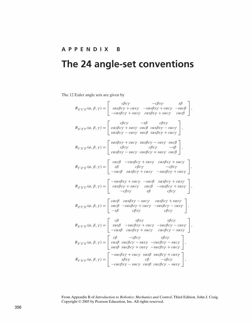
A P P E N D I X B
The 24 angle-set conventions
The 12 Euler angle sets are given by
RX′Y ′Z′(α, β, γ ) =
cβcγ −cβsγ sβ
sαsβcγ + cαsγ −sαsβsγ + cαcγ −sαcβ
−cαsβcγ + sαsγ cαsβsγ + sαcγ cαcβ
,
RX′Z′Y ′(α, β, γ ) =
cβcγ −sβ cβsγ
cαsβcγ + sαsγ cαcβ cαsβsγ − sαcγ
sαsβcγ − cαsγ sαcβ sαsβsγ + cαcγ
,
RY ′X′Z′(α, β, γ ) =
sαsβsγ + cαcγ sαsβcγ − cαsγ sαcβ
cβsγ cβcγ −sβ
cαsβsγ − sαcγ cαsβcγ + sαsγ cαcβ
,
RY ′Z′X′(α, β, γ ) =
cαcβ −cαsβcγ + sαsγ cαsβsγ + sαcγ
sβ cβcγ −cβsγ
−sαcβ sαsβcγ + cαsγ −sαsβsγ + cαcγ
,
RZ′X′Y ′(α, β, γ ) =
−sαsβsγ + cαcγ −sαcβ sαsβcγ + cαsγ
cαsβsγ + sαcγ cαcβ −cαsβcγ + sαsγ
−cβsγ sβ cβcγ
,
RZ′Y ′X′(α, β, γ ) =
cαcβ cαsβsγ − sαcγ cαsβcγ + sαsγ
sαcβ −sαsβsγ + cαcγ −sαsβcγ − cαsγ
−sβ cβsγ cβcγ
,
RX′Y ′X′(α, β, γ ) =
cβ sβsγ sβcγ
sαsβ −sαcβsγ + cαcγ −sαcβcγ − cαsγ
−cαsβ cαcβsγ + sαcγ cαcβcγ − sαsγ
,
RX′Z′X′(α, β, γ ) =
cβ −sβcγ sβsγ
cαsβ cαcβcγ − sαsγ −cαcβsγ − sαcγ
sαsβ sαcβcγ + cαsγ −sαcβsγ + cαcγ
,
RY ′X′Y ′(α, β, γ ) =
−sαcβsγ + cαcγ sαsβ sαcβcγ + cαsγ
sβsγ cβ −sβcγ
−cαcβsγ − sαcγ cαsβ cαcβcγ − sαsγ
,
From Appendix B of Introduction to Robotics: Mechanics and Control, Third Edition. John J. Craig.
Copyright © 2005 by Pearson Education, Inc. All rights reserved.
356
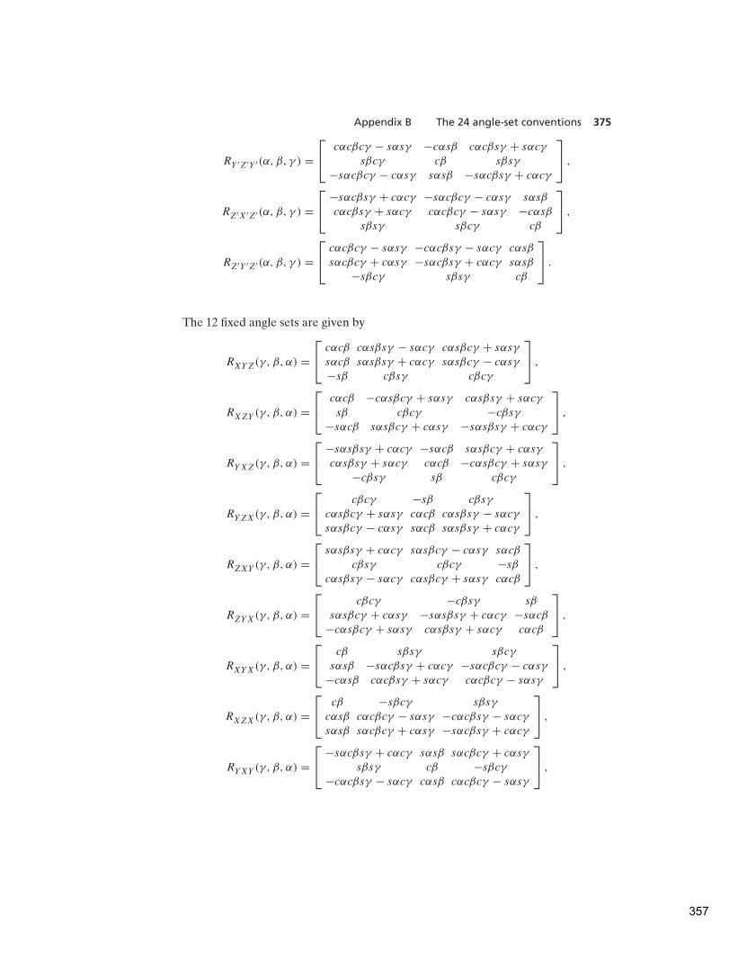
Appendix B The 24 angle-set conventions 375
RY ′Z′Y ′(α, β, γ ) =
cαcβcγ − sαsγ −cαsβ cαcβsγ + sαcγ
sβcγ cβ sβsγ
−sαcβcγ − cαsγ sαsβ −sαcβsγ + cαcγ
,
RZ′X′Z′(α, β, γ ) =
−sαcβsγ + cαcγ −sαcβcγ − cαsγ sαsβ
cαcβsγ + sαcγ cαcβcγ − sαsγ −cαsβ
sβsγ sβcγ cβ
,
RZ′Y ′Z′(α, β, γ ) =
cαcβcγ − sαsγ −cαcβsγ − sαcγ cαsβ
sαcβcγ + cαsγ −sαcβsγ + cαcγ sαsβ
−sβcγ sβsγ cβ
.
The 12 fixed angle sets are given by
RXYZ(γ, β, α) =
cαcβ cαsβsγ − sαcγ cαsβcγ + sαsγ
sαcβ sαsβsγ + cαcγ sαsβcγ − cαsγ
−sβ cβsγ cβcγ
,
RXZY (γ, β, α) =
cαcβ −cαsβcγ + sαsγ cαsβsγ + sαcγ
sβ cβcγ −cβsγ
−sαcβ sαsβcγ + cαsγ −sαsβsγ + cαcγ
,
RYXZ(γ, β, α) =
−sαsβsγ + cαcγ −sαcβ sαsβcγ + cαsγ
cαsβsγ + sαcγ cαcβ −cαsβcγ + sαsγ
−cβsγ sβ cβcγ
,
RYZX(γ, β, α) =
cβcγ −sβ cβsγ
cαsβcγ + sαsγ cαcβ cαsβsγ − sαcγ
sαsβcγ − cαsγ sαcβ sαsβsγ + cαcγ
,
RZXY (γ, β, α) =
sαsβsγ + cαcγ sαsβcγ − cαsγ sαcβ
cβsγ cβcγ −sβ
cαsβsγ − sαcγ cαsβcγ + sαsγ cαcβ
,
RZYX(γ, β, α) =
cβcγ −cβsγ sβ
sαsβcγ + cαsγ −sαsβsγ + cαcγ −sαcβ
−cαsβcγ + sαsγ cαsβsγ + sαcγ cαcβ
,
RXYX(γ, β, α) =
cβ sβsγ sβcγ
sαsβ −sαcβsγ + cαcγ −sαcβcγ − cαsγ
−cαsβ cαcβsγ + sαcγ cαcβcγ − sαsγ
,
RXZX(γ, β, α) =
cβ −sβcγ sβsγ
cαsβ cαcβcγ − sαsγ −cαcβsγ − sαcγ
sαsβ sαcβcγ + cαsγ −sαcβsγ + cαcγ
,
RYXY (γ, β, α) =
−sαcβsγ + cαcγ sαsβ sαcβcγ + cαsγ
sβsγ cβ −sβcγ
−cαcβsγ − sαcγ cαsβ cαcβcγ − sαsγ
,
357
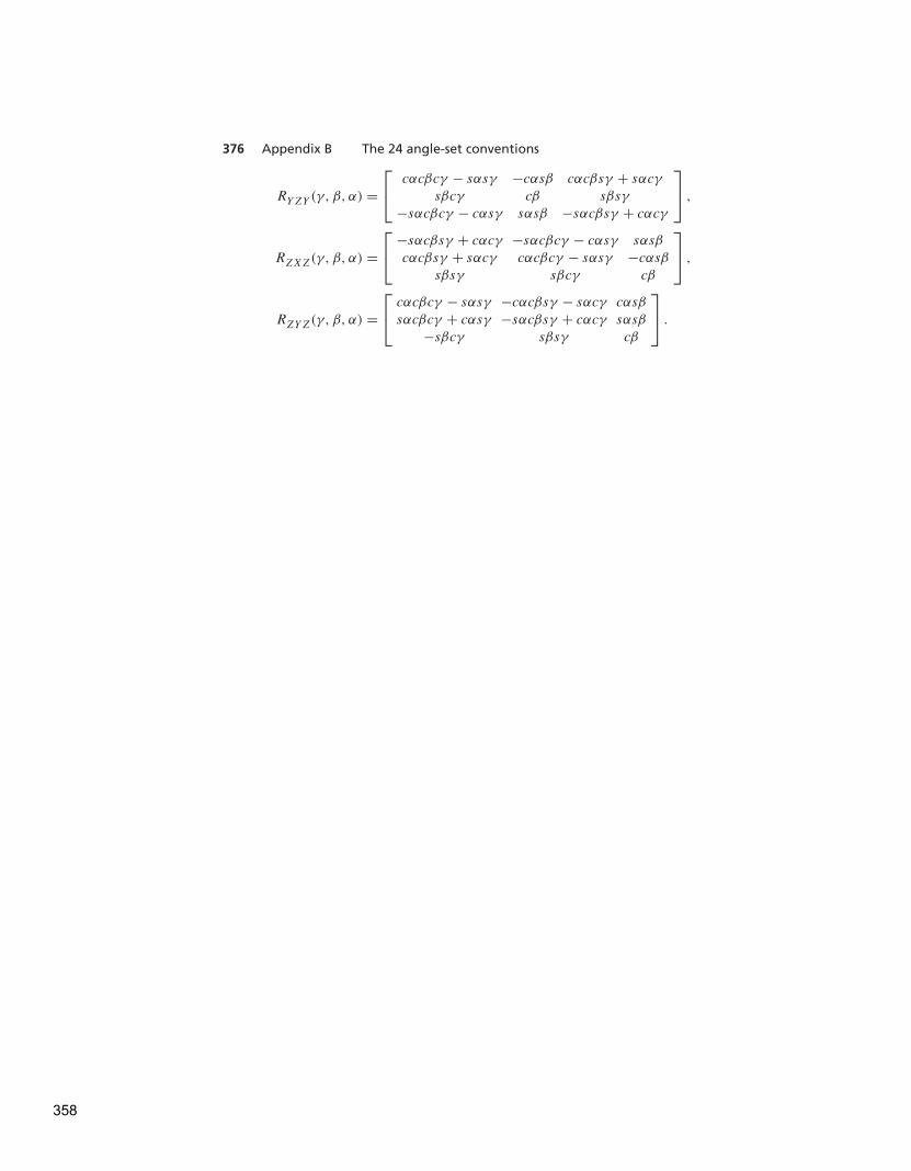
376 Appendix B The 24 angle-set conventions
RYZY (γ, β, α) =
cαcβcγ − sαsγ −cαsβ cαcβsγ + sαcγ
sβcγ cβ sβsγ
−sαcβcγ − cαsγ sαsβ −sαcβsγ + cαcγ
,
RZXZ(γ, β, α) =
−sαcβsγ + cαcγ −sαcβcγ − cαsγ sαsβ
cαcβsγ + sαcγ cαcβcγ − sαsγ −cαsβ
sβsγ sβcγ cβ
,
RZYZ(γ, β, α) =
cαcβcγ − sαsγ −cαcβsγ − sαcγ cαsβ
sαcβcγ + cαsγ −sαcβsγ + cαcγ sαsβ
−sβcγ sβsγ cβ
.
358

A P P E N D I X C
Some inverse-kinematicformulas
The single equationsin θ = a (C.1)
has two solutions, given by
θ = ±Atan2(√
1 − a2, a). (C.2)
Likewise, givencos θ = b, (C.3)
there are two solutions:θ = Atan2(b,±
√
1 − b2). (C.4)
If both (C.1) and (C.3) are given, then there is a unique solution given by
θ = Atan2(a, b). (C.5)
The transcendental equation
a cos θ + b sin θ = 0 (C.6)
has the two solutionsθ = Atan2(a,−b) (C.7)
andθ = Atan2(−a, b). (C.8)
The equationa cos θ + b sin θ = c, (C.9)
which we solved in Section 4.5 with the tangent-of-the-half-angle substitutions, isalso solved by
θ = Atan2(b, a) ± Atan2(√
a2 + b2 − c2, c). (C.10)
The set of equations
a cos θ − b sin θ = c,
a sin θ + b cos θ = d, (C.11)
which was solved in Section 4.4, also is solved by
θ = Atan2(ad − bc, ac + bd). (C.12)
From Appendix C of Introduction to Robotics: Mechanics and Control, Third Edition. John J. Craig.
Copyright © 2005 by Pearson Education, Inc. All rights reserved.
359

This page intentionally left blank
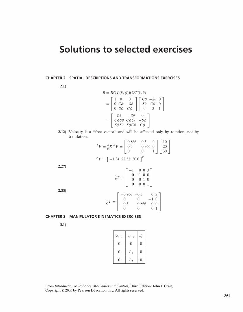
Solutions to selected exercises
CHAPTER 2 SPATIAL DESCRIPTIONS AND TRANSFORMATIONS EXERCISES
2.1)
R = ROT(x, φ)ROT(z, θ)
=
1 0 00 Cφ −Sφ
0 Sφ Cφ
Cθ −Sθ 0Sθ Cθ 00 0 1
=
Cθ −Sθ 0CφSθ CφCθ −Sφ
SφSθ SφCθ Cφ
2.12) Velocity is a ‘‘free vector’’ and will be affected only by rotation, not bytranslation:
AV = A
BR BV =
0.866 −0.5 00.5 0.866 00 0 1
102030
AV =[
−1.34 22.32 30.0]T
2.27)
A
BT =
−1 0 0 30 −1 0 00 0 1 00 0 0 1
2.33)
B
CT =
−0.866 −0.5 0 30 0 +1 0
−0.5 0.866 0 00 0 0 1
CHAPTER 3 MANIPULATOR KINEMATICS EXERCISES
3.1)
αi−1 ai−1 di
0 0 0
0 L1 0
0 L2 0
From Introduction to Robotics: Mechanics and Control, Third Edition. John J. Craig.
Copyright © 2005 by Pearson Education, Inc. All rights reserved.
361
380 Solutions to selected exercises
01T =
C1 −S1 0 0S1 C1 0 00 0 1 00 0 0 1
12T =
C2 −S2 0 L1S2 C2 0 00 0 1 00 0 0 1
23T =
C3 −S3 0 L2S3 C3 0 00 0 1 00 0 0 1
03T = 0
1T
12T
23T =
C123 −S123 0 L1C1 + L2C12S123 C123 0 L1S1 + L2S12
0 0 1 00 0 0 1
where
C123 = cos(θ1 + θ2 + θ3)
S123 = sin(θ1 + θ2 + θ3)
3.8) When {G} = {T }, we have
B
WT W
TT = B
ST S
GT
SoW
TT = B
WT −1 B
ST S
GT
4.14) No. Pieper’s method gives the closed-form solution for any 3-DOF manipula-tor. (See his thesis for all the cases.)
4.18) 2
4.22) 1
CHAPTER 5 JACOBIANS: VELOCITIES AND STATIC FORCES EXERCISES
5.1) The Jacobian in frame {0} is
◦J (θ) =[
−L1S1 − L2S12 −L2S12L1C1 + L2C12 L2C12
]
DET(◦J (θ)) = −(L2C12)(L1S1 + L2S12) + (L2S12)(L1C1 + L2C12)
= −L1L2S1C12 − L22S12C12 + L1L2C1S12 + L2
2S12C12
= L1L2C1S12 − L1L2S1C12 = L1L2(C1S12 − S1C12)
= L1L2S2
∴ The same result as when you start with 3J (θ), namely, the singularconfigurations are θ2 = 0◦ or 180◦.
362
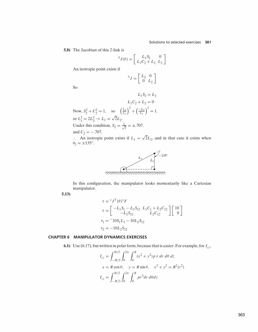
Solutions to selected exercises 381
5.8) The Jacobian of this 2-link is
3J (θ) =[
L1S2 0L1C2 + L2 L2
]
An isotropic point exists if
3J =[
L2 00 L2
]
So
L1S2 = L2
L1C2 + L2 = 0
Now, S22
+ C22
= 1, so(
L2L1
)2+
(
−L2L1
)2= 1.
or L21
= 2L22
→ L1 =√
2L2.
Under this condition, S2 = 1√2
= ±.707.
and C2 = −.707.
∴ An isotropic point exists if L1 =√
2L2, and in that case it exists whenθ2 = ±135◦.
L1L2
�135
In this configuration, the manipulator looks momentarily like a Cartesianmanipulator.
5.13)
τ = ◦J T (θ)◦F
τ =[
−L1S1 − L2S12 L1C1 + L2C12−L2S12 L2C12
] [
100
]
τ1 = −10S1L1 − 10L2S12
τ2 = −10L2S12
CHAPTER 6 MANIPULATOR DYNAMICS EXERCISES
6.1) Use (6.17), but written in polar form, because that is easier. For example, for Izz,
Izz =∫ H/2
−H/2
∫ 2π
0
∫ R
0(x2 + y2)p r dr dθ dz
x = R cos θ, y = R sin θ, x2 + y2 = R2(r2)
Izz =∫ H/2
−H/2
∫ 2π
0
∫ R
0pr3dr dθdz
363

382 Solutions to selected exercises
X
Z
YH
R
Izz = π
2R4Hp, VOLUME = πr2H
∴ Mass = M = pπr2H ∴ Izz = 12 MR2
Similarly (only harder) is
Ixx = Iyy = 14 MR2 + 1
12 MH2
From symmetry (or integration),
Ixy = Ixz = Iyz = 0
∴
cI =
14 MR2 + 1
12 MH2 0 0
0 14 MR2 + 1
12 MH2 0
0 0 12 MR2
6.12) θ1(t) = Bt + ct2, soθ1 = B + 2ct, θ = 2c
so
1ω1 = θ1z1 = 2cz1 =
002c
1vc1 =
002c
⊗
200
+
00θ1
⊗
00θ1
⊗
200
=
04c0
+
−2θ21
00
1vc1 =
−2(B + 2ct)2
4c0
6.18) Any reasonable F(θ, θ) probably has the property that the friction force (ortorque) on joint i depends only on the velocity of joint i, i.e.,
F(θ, θ) = [f1(θ, θ1) F2(θ, θ2) . . . .FN (θ, θN )]T
364

Solutions to selected exercises 383
Also, each fi(θ, θi) should be ‘‘passive’’; i.e., the function should lie in the first& third quadrants.
Fi
�i
.
** Solution written by candlelight in aftermath of 7.0 earthquake, Oct. 17,1989!
CHAPTER 7 TRAJECTORY GENERATION EXERCISES
7.1) Three cubics are required to connect a start point, two via points, and a goalpoint—that is, three for each joint, for a total of 18 cubics. Each cubic has fourcoefficients, so 72 coefficients are stored.
7.17) By differentiation,
θ (t) = 180t − 180t2
θ (t) = 180 − 360t
Then, evaluating at t = 0 and t = 1, we have
θ(0) = 10 θ (0) = 0 θ (0) = 180
θ(1) = 40 θ (1) = 0 θ (1) = −180
8.3) Using (8.1), we have
L =3
∑
i=1
(ai−1 + di) = (0 + 0) + (0 + 0) + (0 + (U − L)) = U − L
W = 4
3πU3 − 4
3πL3 = 4
3π(U3 − L3)
a‘‘hollow’’
sphere
∴ QL = U − L
3
√
43π(U3 − L3)
8.6) From (8.14),
1
KTOTAL
= 1
1000+ 1
300= 4.333 × 10⁻³
∴ KTOTAL = 230.77NTM
RAD
8.16) From (8.15),
K = Gπd4
32L= (0.33 × 7.5 × 1010)(π)(0.001)4
(32)(0.40)= 0.006135
NTM
RAD
This is very flimsy, because the diameter is 1 mm!
365
384 Solutions to selected exercises
9.2) From (9.5),
s1 = − 6
2 × 2+
√36 − 4 × 2 × 4
2 × 2= −1.5 + 0.5 = −1.0
s2 = −1.5 − 0.5 = −2.0
∴
quadx(t) = c1e−t + c2e
−2t and x(t) = −c1e−t − 2c2e
−2t
Att = 0 x(0) = 1 = c1 + c2 (1)
x(0) = 0 = −c1 − 2c2 (2)
Adding (1) and (2) gives1 = −c2
so c2 = −1 and c1 = 2.
∴ x(t) = 2e−t − e−2t
9.10) Using (8.24) and assuming aluminum yields
K = (0.333)(2 × 10¹¹)(0.054 − 0.044)
(4)(0.50)= 123,000.0
Using info from Figure 9.13, the equivalent mass is (0.23)(5) = 1.15 kg,
so
Wres =√
k/m =√
123,000.0
1.15∼= 327.04
rad
sec
This is very high—so the designer is probably wrong in thinking that this linkvibrating represents the lowest unmodeled resonance!
9.13) As in problem 9.12, the effective stiffness is K = 32000. Now, the effectiveinertia is I = 1 + (0.1)(64) = 7.4.
∴ Wres =√
32000
7.4∼= 65.76
rad
sec∼= 10.47 Hz
CHAPTER 10 NONLINEAR CONTROL OF MANIPULATORS EXERCISES
10.2) Let τ = ατ ′ + β
α = 2 β = 5θ θ − 13θ3 + 5
and τ ′ = θD + Kv e + Kpe
where e = θD − θ
and
Kp = 10
Kv = 2√
10
366

Solutions to selected exercises 385
10.10) Let f = αf ′ + β
with α = 2, β = 5xx − 12
and f ′ = XD + kv e + kpe, e = XD − X
kp = 20, kv = 2√
20.
CHAPTER 11 FORCE CONTROL OF MANIPULATORS EXERCISES
11.2) The artificial constraints for the task in question would be
Vz = −a1 Fx = 0Fy = 0
Nx = 0Ny = 0
Nz = 0
where a1 is the speed of insertion.
11.4) Use (5.105) with frames {A} and {B} reversed. First, find B
AT , so invert A
BT :
B
AT =
0.866 0.5 0 −8.66−0.5 0.866 0 5.0
0 0 1 −5.00 0 0 1
Now,
BF = B
AR AF =
[
1 1.73 −3]T
BN = BPAORG ⊗ BF + B
AR AN =
[
−6.3 −30.9 −15.8]T
∴BF =
[
1.0 1.73 −3 −6.3 −30.9 −15.8]T
367

This page intentionally left blank

Index
IndexPage references followed by "f" indicate illustratedfigures or photographs; followed by "t" indicates atable.
AAcceleration, 5, 9, 62, 165-167, 171-173, 176, 180,
185-186, 189, 195, 201, 204-213, 215-216,219, 224-229, 233, 241, 256, 307
Accumulator, 251system, 251
Accuracy, 101, 127, 129, 233, 348-349, 351Actions, 14, 90, 241, 344Activity, 307Actuator, 9, 12, 62, 76-78, 83-86, 89, 95, 121,
124-125, 175, 183, 199, 225-226, 243-245,250-253, 263-264, 271-272, 277-279, 290,295, 297
Adaptive control, 290, 302, 311, 313Addition, 7, 16, 20, 23-24, 28, 174, 216, 235, 242, 261,
271, 277, 285, 288matrices, 16
Advanced, 18, 92, 194, 222, 251, 288, 290, 350Agriculture, 17Air, 251Aircraft, 7-8, 234Algebraic equations, 114Algorithms, 3, 9, 11-12, 105, 191, 210, 313, 339
scope of, 210Aluminum, 248-250, 258, 366Amplitude, 268Analog, 171, 252-253, 278, 285
sensors, 252-253, 278Analog signals, 252Analytical solution, 223and, 1-18, 19-36, 38-48, 50-56, 58-61, 62-86, 89-96,
99-100, 101-133, 165-177, 180-200,201-209, 211-229, 230-236, 238, 240-261,262-275, 277-283, 285-289, 290-291,293-301, 303-316, 339-352, 354-355, 356,359, 361-363, 365-367
Angle, 16, 22, 41, 43-48, 50, 54-55, 58-60, 64-66, 69,72, 75, 82, 85, 92, 94-95, 100, 111, 114, 117,121, 127, 192, 195, 203, 208, 218-219, 229,237, 251-252, 256, 261, 263, 288-289, 344,354-355, 356-358, 359
Angles, 5-6, 41-46, 55-56, 59-61, 77-78, 83-85, 89, 95,99-100, 101, 108-109, 112-113, 116-118,123-128, 130, 132-134, 185, 199-200, 203,205, 217, 219, 223, 252, 256, 261, 354
computing, 5, 43, 95, 101, 127, 205measurement, 128phase, 252
Angular acceleration, 167, 172-173, 195, 229velocity, 172-173, 195, 229
Angular motion, 245Arc, 42-43, 130, 231-232, 255Arc welding, 231-232, 255architecture, 92, 262, 284, 299, 303Arc-welding, 130area, 17, 126, 130, 133, 225, 249, 283, 297Arguments, 43, 60, 100, 120, 132, 183, 301, 341ARM, 9-10, 63, 68-70, 91-95, 100, 101, 103, 109, 112,
121-123, 129, 187, 191-194, 196, 224-227,230, 235-236, 242, 287-288, 296, 298-300,302, 308-314, 316, 348-349, 351-352
Arrays, 18in MATLAB, 18
Artificial, 6, 225-226, 312, 367intelligence, 226, 312
Artificial intelligence, 226, 312ASCII, 18Assembly, 3, 17, 235, 343, 348-349
automated, 343Assumptions, 92, 195, 264, 278, 283-284, 296, 298,
348, 351Attributes, 3-4, 9-10, 15, 19, 63, 202, 221, 230, 239,
251Automated, 15, 339, 342-343, 346
assembly, 343inspection, 343
Automatic, 91, 226, 255, 313Automatic control, 226, 313Automation, 1, 3, 14-17, 193, 226, 233, 255-256,
312-313, 339-340applications, 1, 3, 15, 17, 233, 312, 339-340hard, 233history, 1
Automobiles, 234Availability, 52Average, 208, 288, 302, 315Average value, 288Avoidance, 226Axis, 8-9, 11, 20, 31, 41, 43-44, 46-51, 54-58, 61,
64-72, 75, 86, 92, 96, 108, 110, 121, 123,167-168, 170-171, 184, 199-200, 218-219,221, 231-232, 235-238, 254, 256-257,260-261, 288
BBack, 1, 46, 55, 72, 133-134, 175, 212, 222, 232, 236,
264, 279, 288-289, 343, 348, 350Back emf, 279, 288-289
constant, 279, 288-289Backlash, 245, 252Backward, 30-32Ball, 243-244, 246-247, 257-259Band, 246, 278Bandwidth, 278, 303
aliasing, 278Bar, 5, 65, 77, 83, 121, 253base, 5-6, 14, 16-18, 39, 62-63, 68, 70, 72, 84-85,
89-91, 99-100, 101, 104, 110, 115-116,125-126, 130, 132-133, 175-177, 194,243-245, 257-258, 290, 341, 352
Basic, 3, 5, 7, 51, 83, 126, 202, 264-265, 276, 295,307, 341, 345-346, 350
size, 202Beams, 282-283Bearings, 64-65, 67, 246, 251, 278, 280-281Bed, 130Bend, 246
length, 246radius, 246
Bending, 189, 278force, 278
Bias, 347Biological, 6Black, 297Black box, 297block diagram, 263, 271, 274-275, 285, 292, 298, 310,
314functions, 298, 310
Bottle, 351Bottom, 72, 348Boundary, 241
representation, 241Bounds, 233, 350Bridge, 252
ac, 252
CCables, 246Cabling, 252, 254Calculations, 67, 91, 106, 190-191, 303
automatic, 91Calibration, 94, 127-128, 253Calls, 60, 126, 133, 341, 346, 352carry, 16, 263Case studies, 17Cast, 28, 209Cations, 350Cells, 192Center, 14, 100, 126, 170-174, 177, 182-184, 194-195,
197-199, 241, 256, 260, 286, 299, 302Centrifugal, 180-181, 188, 295Centrifugal force, 181Chain, 5, 16, 38, 62-63, 66, 68, 83, 85, 106, 121, 165,
182, 193, 230, 241-243, 246Chains, 85, 246changing, 4, 6, 19, 24-25, 27, 29, 56, 111, 166, 181,
202, 248, 311Channels, 252Characteristic equation, 265, 267-268, 270Cigarette, 351Circuit boards, 231-232Circuits, 279, 285Circular, 61, 134, 217, 241Clearance, 348CLOCK, 8, 297Closed-loop control, 262-263, 272, 274Closed-loop control system, 272, 274Closed-loop system, 264, 271-272, 276, 292, 294,
296, 300-301, 303, 306Coefficient, 188, 264-265, 288-289, 291
of friction, 188Collection, 3, 339Columns, 21-22, 25-27, 34, 39-41, 54, 92, 218Common causes, 349Communication, 303, 341Communications, 14, 339Complex function, 180component, 11, 16, 22, 116, 175, 199-200, 223, 261,
265, 301type, 301
Compound, 34-35, 38Computations, 53, 77, 173, 190, 192, 216, 277, 285,
296-297, 308Computer, 1, 3, 6, 15, 17-18, 28, 41, 51, 54, 91-92,
114, 127-128, 181, 190, 192, 194, 201, 225,253, 256, 271-272, 277, 284-285, 296-297,299, 301, 309, 311-312, 339-342, 346-348,350
simulation, 15, 190, 194, 297vision, 17, 54, 127, 342, 347-348
Computer-aided, 1, 15computer-aided design, 1, 15Computer-aided manufacturing (CAM), 1Computers, 201, 284, 341Concatenate, 73Conditioning, 241Congress, 128, 192-193Constants, 83-84, 86, 111, 121, 133, 227, 266-267,
273, 289special, 266
Construction, 28, 253Container, 9Continuous, 8, 190, 202-204, 207-209, 211, 219, 227,
262-263, 277-278, 296-297, 299, 304-305path, 202-204, 207, 209, 211, 219
Contrast, 342Control, 1, 3-7, 9, 11-13, 15, 17-18, 19, 62, 89, 92, 94,
101, 125, 127-128, 165, 181, 192-194,198-199, 201, 221-222, 224, 226, 230-231,242, 251-253, 255, 260-261, 262-266, 268,270-289, 290-304, 306-316, 339-343, 345,347, 349-351, 354, 356, 359, 361, 366-367
adaptive, 255, 290, 311-313numerical, 101, 127, 193, 198, 252, 286-287, 297,
308segment, 222, 224, 345, 349
Control law, 13, 271-275, 277, 282, 284-285, 287, 291,293-297, 299-303, 306-307, 312, 315-316
Control systems, 12-13, 125, 221, 224, 262, 264, 277,288, 290, 295, 297, 301, 303, 307, 309, 349
robots, 12-13, 301, 307, 349controllability, 245, 251
output, 245, 251Controller, 230, 262-263, 273-276, 281, 284-285,
287-289, 290-291, 294-295, 298, 300-301,303, 306, 309-310, 312, 314-316, 342,
369

346-347, 350Controlling, 9, 13, 165, 290, 295, 345Controls, 83-84, 284Conversion, 60, 86, 307-308, 310Cooling, 252Coordinate systems, 4, 16, 19-20, 24Coordinates, 6, 56-57, 71, 76, 115, 121, 127, 261, 285,
307, 347, 351adjusting, 285
Corners, 58-59Correlation, 278cost, 1, 9, 17-18, 91-92, 192, 230, 245Costs, 1-2, 17-18
labor, 1-2, 17-18material, 1product, 18
Coulomb friction, 188, 293Cranes, 234
gantry cranes, 234Critically damped motion, 270
response, 270Critically damped system, 270Cross, 18, 21, 92, 108, 245, 249, 253, 287, 303cube, 240Curves, 17, 213, 225Cycles, 252, 284Cylinders, 250-251
DDamper, 305Damping, 266, 268, 272-275, 280, 287-289, 290-291,
302-303, 316critical, 266, 268, 272-275, 287, 291, 302, 316models, 291, 303
Damping ratio, 268data, 15, 17-18, 55, 99, 210, 222-223, 260, 345, 347Deburring, 231Decade, 1Decisions, 231, 345Defects, 342
surface, 342Deflections, 230, 247, 249, 251, 256Degree, 5, 8-9, 18, 63, 103, 106-107, 114, 116, 167,
195, 201, 204, 219, 223, 225, 231, 242-244,255, 258, 260, 265, 286, 290, 314, 340, 348
Degree of freedom, 5, 9, 18, 63, 167, 201, 219, 223,225, 231, 255, 340
Degrees of freedom, 5, 7, 9, 51, 59, 63, 71, 76-77, 83,92, 101-103, 105-109, 112, 114, 117, 121,180, 219, 231-232, 234, 241-244, 256-259,295, 314
multiple, 7, 102-103, 106delay, 297density, 168-169, 194, 199Design, 1, 3, 10-12, 15, 17, 52, 63, 74, 77, 80, 106,
128, 225, 230-234, 236-242, 244-248,250-256, 258, 260, 264, 273-275, 281,285-287, 289, 290-291, 293-294, 302, 310,312, 314-316, 339, 345, 351
attributes, 3, 10, 15, 63, 230, 239, 251Design considerations, 63Design decisions, 231, 345Design for, 255, 285design time, 241Determinant, 39-40, 59, 241, 258, 260Diagrams, 288Differential equations, 262, 265, 285, 290, 297, 304Digital, 201, 277-278, 285, 296-297, 313
signals, 297Digital circuitry, 297Dimension, 40, 188, 192, 241Direct, 7, 15, 53, 101, 193, 244, 251-252, 255, 266,
278, 281, 286-287, 302, 304, 312-313, 349Discrepancies, 347Discrete-time systems, 297Displacement, 5, 309Distances, 20, 168
perpendicular, 168Distribution, 165, 167-169, 171, 173, 177, 190, 230,
245Disturbance, 254, 262, 272, 276-278, 289, 299-300,
304, 309, 311documentation, 350Dot product, 22, 26Double, 66, 69Draw, 55, 60, 69, 314Drawing, 74, 253Drilling, 348driver, 279, 285
dual, 298, 310Dynamic systems, 17, 128, 192, 194, 251, 285, 313
EEconomics, 1, 10Effective mass, 282-283Efficiency, 127, 190-191, 240Eigenvalues, 54, 58, 171, 241, 258Eigenvector, 54Eigenvectors, 171, 241Elasticity, 248-250
modulus of, 248-250Electric, 9, 251, 257, 279Electromechanical, 288Electrons, 278Elements, 15, 20, 40, 76, 117-120, 123, 132, 168, 171,
218, 225, 230, 245-248, 250, 253, 281frame, 20, 40, 76, 132, 168, 171, 218, 247, 253
Elevation, 7-9, 56, 235Ellipsoid, 241Encoder, 252, 284-285, 288-289
binary, 252End-of-arm tooling, 230energy, 182-184, 278, 283, 303-304
kinetic, 182-184, 303limited, 278potential, 183-184, 303work, 304
Engineering, 3, 16, 54, 192, 231, 255-256, 265, 286computer, 3, 54, 192, 256industrial, 3value, 192
Engineering design, 255, 286Engineers, 17, 255Engines, 255Entity, 19, 23, 26, 52, 230Equations, 5, 7, 9-10, 18, 19, 28, 31-32, 37-38, 42, 64,
76-77, 83, 85-86, 89, 91-92, 95, 101-103,105-106, 109-114, 116-122, 127-129,131-133, 165, 173-183, 185-186, 188-191,193-198, 204, 207, 209-210, 213, 223, 227,229, 230, 245, 260, 262, 264-265, 277, 285,290-291, 295, 297-298, 303-304, 307-308,310, 314-315, 359
laws, 277, 297, 307Equilibrium, 304Equipment, 1, 15, 251, 339, 346-347Error, 127, 221, 252, 257, 264, 275-277, 281, 285,
287-288, 296, 298-302, 307, 309-310, 314,316, 346, 349-350
reading, 285scale, 221
Errors, 11, 127, 264, 272, 275-276, 295, 298, 300-302,307-310, 312, 316, 349-350
Estimating, 250, 282-283Estimation, 127, 283Euler method, 182European Union, 2Evaluation, 93-94, 128, 230event, 346-347, 350Events, 17, 346Experiments, 192, 286
FFactors, 129, 230-231False, 132Feedback control, 251, 285, 288, 313Feedforward control, 297Field, 9, 106, 165, 225, 250, 252, 265, 277-278, 290,
297Figures, 38, 100, 133, 198-199, 260Fine, 199-200, 242, 252, 261Finite element method, 255Firing, 8Fit, 199, 205, 254, 261Flat, 11, 67, 258Flexibility, 230, 245-246, 250, 254, 281-283, 287Flexible, 1, 14, 192, 246-247, 281-282, 286, 339
automation, 1, 14, 339Flexure, 253-254Floating-point numbers, 341Fluid, 251Foil, 253-254Force, 3, 9-11, 13, 18, 51-52, 94, 104, 172, 174-175,
181-182, 186, 216, 229, 230-231, 241-242,244, 249, 251-255, 264, 271, 276-279,292-293, 306, 309-310, 313, 341-343,347-351, 364, 367
body, 172, 174, 230, 264, 271, 310centrifugal, 181
Forcing function, 276Forming, 37, 53, 81, 88, 119, 225, 308Frames, 4, 19, 21, 23-27, 29-31, 34-35, 38, 44, 48, 51,
55, 58-60, 62, 67-76, 78, 87, 89-92, 94-96,100, 101, 107, 115, 121, 125-126, 133, 178,186, 190-191, 202, 217, 224, 228, 344, 346,352, 367
moments in, 190framework, 34, 198Free space, 13, 175, 225-226Free-body diagram, 174, 264, 271Frequency, 268, 277-279, 281-283, 287, 308
damped, 268, 281-282reference, 278
Friction, 9, 188-189, 194-198, 230, 245-246, 251-252,264-266, 273, 280, 290-291, 293, 295,299-300, 303, 313, 364
Full, 9, 35, 43, 102-103, 108, 225, 231, 254, 343, 351Functions, 9-10, 16, 18, 43, 61, 77, 92, 100, 132-133,
180-183, 192, 199, 201, 203, 205, 210-212,217-218, 229, 245, 261, 273, 298, 301, 305,310-311
sinusoidal, 217
GGain, 274, 276, 289, 298, 306, 309-310Gains, 272-274, 281-284, 287-289, 291-295, 298, 302,
308-310, 314-315Gantry cranes, 234Gantry robots, 234Gears, 189, 237, 245, 248-250, 256-257, 287
bevel, 237, 245General, 5, 16-17, 27-28, 31, 33-34, 36, 41, 45-47, 55,
58, 68, 72-75, 89, 91, 102-106, 108-110,114, 121-122, 125, 127-128, 132, 167, 182,185, 187-188, 191, 195, 201-202, 205, 207,209-210, 218, 226, 230, 241-244, 256, 258,286, 290, 294, 297, 300, 304, 309, 313,340-342, 351
Generation, 10, 14-15, 92, 193-194, 201-204,206-208, 210, 212, 214, 216-218, 220,222-226, 228-229, 365
Generator, 216, 222-223, 226, 228, 263, 275, 279Geometric, 10, 59, 101, 106, 109, 111-114, 117, 121,
123, 127-128, 199, 201, 219, 221, 226, 254,344-346
modeling, 344-345Geometry, 62, 85, 91, 108, 112-113, 171, 255, 285Glass, 13, 351Goals, 103-104, 108, 110, 126-127, 133, 346graph, 17, 61, 199-200, 225, 261, 289Graphs, 227Gravity, 176, 178, 180-181, 183, 186, 195-196, 199,
227, 247, 289, 293, 295, 300, 302-303, 307,310
Greater than, 289Grinding, 231Group, 190Gun, 7-8
HHand, 6, 11, 14, 20, 22, 36, 39, 41, 44, 46-47, 51,
64-65, 68-69, 71-72, 90-91, 104, 108, 110,116-120, 123, 129, 133, 166, 199-200, 240,243, 258-259, 261, 300-301, 310, 340, 344,349-351
Handling, 1, 231Hard, 40-41, 230, 233, 279, 303Hard automation, 233Head, 8, 23Heading, 60, 93-94, 99Height, 51, 56, 183, 240Help, 18, 26, 221, 242, 342History, 1, 201, 227, 287Homogeneous solution, 261HP, 364Human, 1-2, 6-7, 9, 13-14, 17, 41, 51, 190-191, 201,
233, 339, 351interface, 13, 201, 339
Humans, 51Hybrid, 13, 313Hydraulic, 9, 250-251Hysteresis, 254
IIBM, 341
370

Identity matrix, 22-23, 170, 301, 315IEEE, 17, 128, 193-194, 226, 242, 255-256, 285,
312-313Impact, 253Incomplete, 303Index, 171, 240, 252, 256, 258inductance, 279, 281, 283, 289Industrial, 1-3, 5, 7, 12-13, 15, 17-18, 52, 62, 77-81,
83, 85, 87, 92, 106, 115, 117, 127, 217, 219,221, 226, 232-234, 236, 238, 251-252,262-263, 278, 281, 283-285, 290, 297, 299,301, 307, 313, 339-343
Industrial controllers, 297Industrial robots, 1-3, 5, 12, 17-18, 62, 77-81, 83, 85,
87, 92, 115, 117, 127, 219, 226, 232, 236,238, 251, 263, 278, 285, 301, 307, 313, 339,341, 343
Inertia matrix, 295, 299-300, 303Information, 16, 18, 20, 22-23, 25, 30, 34, 167, 173,
192, 199, 222, 225, 228, 253, 271, 304, 308,345, 347-348
Initial conditions, 189, 265-267, 269-270, 277, 297,304, 348
Initial point, 214-215, 227, 229initialization, 341Input, 14, 60-61, 99-100, 104, 126, 132-133, 189, 191,
224, 245-246, 248-250, 256-258, 264,271-274, 276, 278, 282, 287-289, 290, 295,297, 308, 313, 347
Inputs, 14, 60, 228, 278, 307Inserts, 94Instability, 272Installations, 2-3integer, 219Integrated, 347Integration, 189, 191, 198, 287, 297, 347, 364Integrator, 288Interconnection, 66Interest, 4, 42, 242, 253, 288, 297, 344, 347Intermediate, 10, 28, 44, 66, 68, 74-75, 192, 202, 205,
207-208, 220-221shape, 10
Internal, 6, 11, 60, 201, 230, 253-254, 347-348Interpolation, 210-213, 218-219Inverse problem, 42, 47, 61Inverted pendulum, 294Isolation, 348-349Iterative process, 231
JJoining, 95, 112
KKinetic energy, 182, 184, 303
LLabel, 199-200, 261Labor, 1-2, 17-18Labor costs, 1-2, 18Lag, 252, 308Laplace transforms, 265, 288Laser, 256Laws, 273, 277, 297, 301, 307, 312
Per, 301Lead, 112, 246-247, 349
screw, 246Lead screws, 246-247Leading, 1, 16, 20-22, 26, 168Less than, 8, 113, 304, 348Less than or equal to, 113Lifting, 9Light, 252Limits, 102, 104, 107, 121, 123, 125, 129, 131, 221,
225, 233, 235, 237-238, 240, 256, 261Linear, 11-13, 18, 19, 22, 40, 54, 77, 83-84, 105, 114,
166-167, 173-175, 182, 192, 195, 205, 207,209-219, 221-224, 226-227, 243, 246-247,250, 258-259, 262-270, 272, 274, 276, 278,280, 282, 284, 286, 288, 290-291, 293-294,303, 305
Linear algebra, 18, 22, 40, 54, 192Linear approximation, 262Linear interpolation, 210-211, 213, 218linear region, 216Linear time-invariant system, 291Linearity, 252, 254Lines, 51, 64-66, 69, 95, 103-104, 112, 208, 218-219,
252, 263-264, 307
List, 46, 129, 260Loading, 176, 233, 247, 250, 253, 351Loads, 192, 246-247Local Variables, 91Logic, 340-341Loop, 37, 242-243, 246, 259, 261, 262-265, 271-274,
276, 281-284, 287-288, 291-294, 296-301,303, 306, 308, 310, 315-316
closed, 242-243, 246, 259, 262-264, 271-272, 274,276, 281-284, 287-288, 291-292, 294,296, 298-301, 303, 306, 310, 315-316
Looping, 346Loops, 18lot, 346Lower, 62-63, 65, 92, 104, 114, 175, 188, 245, 252,
256, 278, 281, 308Lubrication, 65, 189
MMachine, 235Magnetic, 251-252, 278Maintenance, 299Manipulators, 1, 3-7, 9-11, 13-17, 54, 62-63, 101, 103,
106, 112, 114, 117, 121, 127-128, 165, 171,180, 188, 190-193, 226, 231, 233-234, 236,240-242, 247, 250-252, 255, 257, 262, 264,266, 268, 270, 272, 274, 276, 278, 280-282,284, 286, 288, 290-296, 298, 300-302, 304,306-308, 310, 312-314, 316, 339, 341-342,348, 351, 366-367
Manual, 18, 350Manufacturing, 1, 15-16, 233, 254-255, 342, 350Mapping, 6-7, 24-28, 30-31, 34, 43, 61
projections, 26Mass, 9, 165, 167-174, 177, 180, 182-184, 186-187,
190, 192, 194-199, 230, 241, 256, 264-265,268, 271, 273-275, 282-283, 287, 289,290-291, 293-294, 299, 303, 306, 310,314-315, 364, 366
Mass matrix, 180, 182-183, 186, 197, 241, 303, 306,310, 315
Material, 1, 3, 63, 165, 168, 240, 254, 262, 339cost, 1handling, 1
Materials, 251Mathematical models, 193MATLAB, 18, 60-61, 100, 133-134, 198-199, 229,
260-261, 288-289M-Files, 18programs, 18
Matrices, 16, 18, 21-22, 29, 31, 33, 36, 39-41, 46,53-56, 58, 60, 76, 81, 86, 92, 95, 100,175-176, 181-182, 192-193, 218, 295-296,301, 306, 346, 355
addition, 16definition of, 21, 29, 58, 100determinant of, 39elements of, 40, 76identity, 22, 301inverse of, 22, 36row, 16, 60square, 95, 181transpose of, 16, 22unit, 21-22, 39-40, 46, 55, 95, 218, 295, 355
Matrix, 7, 9, 16, 18, 21-23, 25-28, 30-34, 39-42, 44-55,57-61, 81, 92, 99-100, 101, 122, 168, 170,177, 180-183, 186, 188, 196-197, 209, 218,241, 253, 260-261, 295, 299-301, 303,305-306, 310, 315
relationships, 49, 51, 53Matrix inverse, 260Matrix multiplication, 26, 57, 81Mean, 6, 116, 300Measurement, 17, 128, 192, 194Measurements, 233, 253-254Mechanical, 1, 3-5, 7, 9-13, 15-17, 63, 65, 74, 92, 124,
182-183, 192-194, 226, 253, 255-256,264-265, 271, 280, 286, 289, 290, 302, 305,313-314
memory, 92, 100, 192, 195, 298, 313, 340Metal, 65, 253-254Metals, 254Meter, 198, 260Method of, 9, 35, 41, 54, 102, 105, 108-109, 112, 117,
122, 246, 283, 290, 297, 303variables, 105, 117
Methods, 1, 12, 61, 67, 105-106, 111, 117, 128, 133,165, 189, 191, 193, 201, 203, 217, 222, 225,230, 262, 290, 297, 308, 349
Microphone, 351Milling, 3Milling machines, 3Mobile robots, 226model, 188-189, 193-194, 197, 201, 224, 233,
249-250, 256, 263, 273, 275, 278-283, 288,290-303, 310-313, 316, 344-345, 347-348
components, 279, 299, 303, 347elements, 250, 281mathematical, 193, 291, 313
Modeling, 190, 262, 278-279, 281-283, 312-313,344-345
Models, 12, 189, 193, 225, 264, 283, 291, 297, 300,303, 307, 312, 345
Modulus of, 248-250Modulus of elasticity, 248-250Moment of inertia, 167, 171, 195, 293Moments, 168-171, 182, 185, 190, 196Moments of inertia, 168-169, 171Motion, 4-5, 7-11, 13-14, 17, 62-63, 91-92, 103-104,
120, 124-126, 133, 165-167, 171-173,175-176, 182-184, 187-191, 193-194,196-200, 201-203, 205, 210-212, 217-221,224-226, 232, 240, 242-243, 245-247, 255,261, 263-271, 273-275, 281, 285-286, 288,290-291, 295, 297-298, 302-303, 307, 310,313, 345-352
equations of, 9-10, 92, 165, 182-183, 189-191,193-194, 196-197, 264, 291, 295, 303,307, 310
relative, 5, 8, 14, 62-63, 91, 125-126, 133, 167,183, 190, 198, 201-203, 205, 217-218,232, 240, 275, 346-347, 352
translational, 347Mounting, 65, 245, 250
NNatural, 13, 15, 40, 165, 241, 268, 271, 277-279,
281-282, 313Natural frequency, 268, 277-279, 281-282Natural response, 271Newton, 165, 171-175, 177, 180, 182, 190, 193, 196,
198-199Noise, 252, 254-255, 263, 275-276, 278, 299, 308Nonlinear system, 294, 303, 315-316Nonlinear systems, 273, 290, 297, 303-304, 313Normal, 64-65, 68-69, 95, 121, 171, 199, 232, 235,
260, 315Not equal to, 130, 309Notation, 1, 16, 21, 25-26, 28, 30-31, 35-36, 39, 44,
46, 67, 70-71, 75, 92, 116, 166, 183, 212,300-302
Numbers, 1, 6, 20, 40-41, 50, 60-61, 64, 67, 110, 216,218, 267, 341
floating-point, 341Numerical solutions, 106
OObjects, 4, 7, 19, 243, 299, 344-345, 347-349Observations, 312Obstacles, 104, 192, 225, 242, 342Offset, 5, 27, 48, 66-67, 72, 86, 92, 240Offsets, 71-72, 91, 102, 191, 234One, 3-5, 7-9, 13, 21, 23-24, 28, 30, 33, 35, 38, 40-41,
43, 45-46, 50-51, 53, 56, 59, 61, 62-63,65-66, 71, 74, 83-85, 91-92, 101-109,111-113, 117, 120-121, 125, 127, 129-130,133, 165, 167, 170, 173, 175, 180, 188-192,195-196, 202, 212, 214, 216-222, 225, 228,231-232, 235-237, 240-242, 246-247, 249,252-254, 257, 260, 263, 265-266, 268,271-272, 276-277, 285-286, 290, 293-294,298-299, 301-304, 309, 312, 314, 339,345-346, 348-351
Open, 5, 83, 193, 265, 272-274, 288, 291, 293, 316Optical, 252, 284, 288Optimization, 92, 194, 226, 254-255, 261, 286
constraints, 226Optimum, 255Order, 4-5, 9-13, 21, 24, 26, 28, 35, 38, 41-42, 44-46,
53-54, 57-58, 62-63, 67, 69, 71-72, 74, 100,109-111, 113, 121, 126-127, 171, 173, 188,201, 203, 209, 211, 225, 229, 232-233, 238,252, 254, 258, 262, 264-273, 275, 277-279,281, 283-284, 286, 290, 297, 304-306,308-310, 348-349
Orientation, 4-7, 19-26, 28-29, 34, 39-41, 43-51,55-56, 62-63, 73, 76-77, 83-85, 89, 91-92,
371
95, 100, 101-105, 107-108, 110, 113, 116,121-122, 127, 129, 169-171, 173-174, 186,196, 201-203, 205, 217-219, 223-224, 227,231-232, 237, 242-243, 257-258, 260, 310,342, 347
Out of, 26, 71, 103, 113, 235, 252, 298, 342, 349-350Output, 60, 91, 99, 228, 244-246, 248, 250-253,
256-258, 264, 271-272, 276, 278-280,287-288, 290, 295, 313, 342
Output control, 290, 295overdamped, 266, 268, 281, 302, 304Overdamped motion, 266Overdamped system, 266Overhead, 8, 234
PPainting, 233, 348Pallet, 342-343, 351Pallets, 343, 351Parabola, 205Parallel processing, 346Parallelogram, 63Parameters, 11, 22, 40, 46, 50, 63-67, 69-74, 76,
78-80, 86, 88, 92, 95, 100, 102, 104-105,108-109, 127, 131-133, 181, 193, 198-199,212, 226, 233, 260, 265, 268, 272-274,288-289, 291, 294, 298-299, 301, 310-313
Parts, 1, 4-5, 13, 19, 33, 62, 101, 130, 175, 232, 244,258, 273, 294, 299, 339, 344, 351
Pascal, 55, 60, 129, 341, 352Peak time, 288Pendulum, 171, 294
inverted, 294Performance analysis, 303Performance specifications, 264Period, 198, 278Permanent, 278pH, 128, 192-193PID controller, 288pin, 90-91, 126, 343-345, 348Pipes, 232Pitch, 41, 55Planning, 17, 201-202, 218, 221, 223-226, 228, 342,
351Plots, 199-200, 227, 229, 261Plug, 134Point, 6, 8-9, 11, 14, 20-24, 26, 30, 34, 48, 50-52,
55-56, 59, 66-67, 69, 72, 78, 80, 83-84,90-91, 95, 102-104, 106, 108, 110, 113-115,121, 123, 125, 127, 130, 133, 165, 177, 182,191-192, 194-196, 203, 205, 207-208,211-212, 214-221, 223-229, 234, 240-241,249, 254, 256-259, 283, 285-287, 291, 293,298, 304, 306, 339-342, 345, 363, 365
Points, 7, 10, 14, 20-21, 30, 38, 58, 68, 85, 103, 108,110, 127, 176, 201-203, 205-210, 212-218,220-221, 224-226, 228-229, 241-242, 258,277, 285, 287, 297, 345, 352, 365
Polar coordinates, 71Polishing, 231Positioning, 7, 9, 130, 231-232, 234, 240, 242, 256,
302Positive definite matrix, 182, 305Potential energy, 183-184, 303Power, 9, 52, 230, 233, 251, 278, 297, 301
static, 9Power consumption, 230Press, 17, 54, 128, 193, 225-226, 254-255, 286,
312-313, 342-343, 351primary, 11, 235, 253Primitives, 345-347, 352Principal, 21, 23, 25, 34, 46, 169, 171, 225, 354Procedures, 55, 106Process, 1, 15, 231, 233, 287, 299, 307-308, 311-312,
339, 342-344, 346, 350capabilities, 350information, 308
Processing, 254, 346Product, 15, 18, 21-22, 26, 38, 54, 81-82, 88, 92, 95,
108, 122, 181, 188, 196, 258Production, 15Productivity, 346Products, 18, 37, 168-171, 181, 188Profile, 201, 205Profitability, 17Programmable, 3, 14-15, 231, 339, 347Programming, 3, 13-15, 18, 43, 59-60, 89, 99,
132-133, 197, 201, 224-226, 228, 260, 285,287, 316, 339-342, 344-352
language, 13-15, 18, 43, 201, 224, 285, 339,341-342, 344-351
Programming languages, 224, 339-342, 344-350, 352Programs, 15, 18, 191, 340-341, 344, 348-350, 352Projections, 22, 26Propagation, 173Property, 60, 182, 246, 276, 364Pull, 1, 246Pulley, 246, 258, 260Pump, 251Pumps, 251
QQuality, 1-2, 10, 224, 252Quantity, 7, 16, 24, 53, 67
RRadian, 248, 250, 256-257, 282, 287Random sampling, 226Range, 8, 43, 91, 113, 121, 124, 129, 192, 240,
242-243, 254, 264, 281, 287, 349argument, 43, 113, 281
Rapid, 1, 340-341, 350Rate control, 198, 260, 310Reaction, 13, 343Reading, 54, 77, 94, 192, 251, 285, 297, 313Reasonable, 104, 189-190, 197, 207, 228, 262, 279,
287-288, 297, 351, 364Record, 287Recovery, 349-350Reduction, 101, 113, 244-248, 251, 253, 256-258, 280,
282, 287Redundant, 92, 128, 230-231, 241-243, 255, 260, 286,
313Reference coordinate systems, 24Rejection, 254, 262, 276, 278, 309, 311Relationships, 49, 51, 53, 62, 111, 175, 245, 268Relative motion, 5, 63Repeat, 45, 174, 198, 287, 316, 346Repeatability, 101, 127, 129, 230, 233Representation, 6, 19, 23, 28-29, 38-41, 43-52, 55, 60,
69, 91, 201, 218-219, 223, 225-227, 241requirements, 127, 230-231, 233, 339, 344-345reset, 223, 350Resistance, 254, 279, 289Resolution, 252
potentiometers, 252Resolver, 252Resonance, 278, 281-283, 287, 366Resonant frequency, 282-283Response, 266-271, 275, 277, 281, 302-304, 310, 347Retrofitting, 235Ring, 102rise, 189, 282, 288rise time, 288Riveting, 348Robotic, 1, 19, 67, 194, 226, 233, 255, 341Robustness, 128, 313Roll, 41, 55, 71, 232, 238Rotary, 5, 77, 104-105, 129, 205, 226, 246-247, 252,
278encoder, 252
Rotation, 4, 9, 16, 21-23, 25-29, 31-34, 36, 39-61, 66,74-75, 92, 99-100, 101, 116, 121-122, 167,175, 178, 218-219, 231, 235, 252, 260, 346,354-355, 361
Rotational motion, 167Rotations, 19, 30-31, 33-34, 40-46, 48, 53-58, 218Rules, 230, 238
SSample, 273, 277-278, 297, 339, 342-344, 347
repeated, 342Sampling, 226, 297, 308Sampling frequency, 308Sampling rate, 297Scale, 86, 221, 229, 233, 279, 289Scope, 1, 50, 106, 189, 210, 241, 250, 261, 297, 312Screw, 63, 246
threads, 246Second-order system, 266-268, 270, 277Seconds, 198, 200, 205-206, 213, 215, 224, 226-227,
229, 352Segments, 207, 209, 214-215, 223-224, 228Semiconductor, 253-254Sensing device, 252Sensor, 12, 14, 127, 252-254, 263, 271-272, 278,
346-347
Sensors, 3, 5, 10-12, 14, 76-77, 94, 127, 230, 235,247, 252-254, 263-264, 271, 278, 297, 339,346-348
semiconductor, 253-254Servo system, 301, 349Shape, 10, 64, 201, 203, 210, 217-219, 233, 345, 349Shear, 248Shear modulus, 248Shearing, 255Side, 36, 44, 85, 110, 116-120, 123, 166, 216, 234,
236-237, 248, 280, 300-301, 354Signal processing, 254Signals, 252, 264, 295, 297, 343Signs, 43, 69, 96, 111, 113, 120Silver, 191, 193SIMPLE, 7, 16, 24, 28, 30-31, 35, 61, 63, 65, 67,
70-71, 74, 83, 86, 91, 102, 109, 114,116-117, 127-129, 173, 175, 177, 181,188-191, 198, 201, 203, 207, 211-212, 218,226, 228, 234, 243, 249-250, 264-265,273-274, 282, 284, 287, 290, 294-295,300-304, 307, 340, 343, 346-347, 349,351-352
Simulation, 9, 15, 165, 189-191, 194, 198-200, 260,264, 287-288, 297, 352
purposes, 264steps, 189, 260
Simulink, 18, 288-289Single, 1, 5, 28, 43, 45, 59, 63, 76-77, 102, 104, 106,
113, 167, 174, 180, 195, 203-206, 211-212,218, 224, 226-229, 246, 249, 254, 257-258,262-264, 273, 278-279, 281, 283-284, 288,290, 293, 346, 359
Singular, 8, 120, 130, 187, 207, 220, 238, 241-242,362
Singular points, 241Sinusoids, 218Sizing, 233, 250Sketches, 100Slope, 208, 212, 214socket, 94, 243-244, 257-259Software, 18, 52, 91, 194, 226Solid, 20, 77, 112, 170, 194, 199Sources, 250, 282specification, 41, 46, 103, 108, 110, 125-126, 133,
208, 216, 218, 224-225, 292-294, 345, 347,351-352
spin, 8Spinning, 231Spraying, 233Springs, 259Square, 42-43, 45, 94-95, 110, 118, 181, 241,
248-249, 252, 287Stability, 276, 290, 297, 301, 303-307, 309, 311-313,
316BIBO, 276
Stability analysis, 290, 301, 303-305stable, 264, 271, 276, 304-307, 309-310, 312, 315-316Stack, 21, 25Standard, 62, 89-92, 101, 125-126, 128, 285, 341,
344, 348, 351standards, 128State equation, 276State space, 192, 313Stationary, 252Statistical, 278Statistics, 17Steady state, 277Steady-state error, 276-277, 281, 316Steel, 199, 248-250, 256, 287Step size, 198Stiffness, 10, 12, 63, 230, 242, 246-251, 253, 255-260,
264, 266, 272-274, 278, 281-283, 287, 291,315, 347, 366
Stops, 226, 253-254Straight lines, 218, 307Strain gauges, 253-254Strategies, 106, 251, 313, 347-349
changes in, 349location, 349
Strength, 63, 65bearing, 65
Structure, 10, 28, 35, 107, 110, 127, 165, 176,180-181, 190, 230, 234-235, 238, 240, 244,247, 253-255, 257, 273, 294, 299, 307, 312
sensitive, 253Structures, 63, 230, 234, 241-243, 253-254Substitution, 31, 114, 116, 119, 266, 269, 354Surface, 9, 13, 125, 232, 342
372

Surfaces, 13, 63, 67, 345Swing, 8Symmetry, 113, 171, 231-232, 238, 364Synthesis, 12, 283, 291, 350System, 4, 6-7, 9, 11-16, 19-21, 23-25, 30-33, 43, 48,
51-52, 56-57, 69, 83, 85, 89-92, 104, 116,125-127, 169-170, 183, 194, 201-202,207-208, 215-216, 218, 221-222, 224-225,228, 230, 232-233, 245-248, 250-251,255-260, 262-289, 290-296, 298-310, 312,314-316, 342, 345-347, 349-352
analogous, 183, 310
TTail, 23Tangents, 207-208Tasks, 1, 11, 13, 91, 127, 230-233, 236, 241, 256, 342temperature, 254Terminals, 340Test, 55, 60-61, 133, 198, 287, 289, 349Testing, 256-257, 340-341, 346, 349-350Thickness, 199, 249, 287Third-order polynomials, 229Three-dimensional, 4, 11, 40, 344Tolerances, 233Tool, 5-6, 14, 34, 51, 62, 89-91, 94, 100, 101, 103,
107-108, 121-122, 125-126, 133, 186,201-203, 205, 207, 217-218, 228, 231-232,238, 247, 299, 344, 352
Tools, 3-4, 13, 19, 91, 112, 265, 297, 299Top, 91, 234-237, 284Total, 53, 104, 106, 117, 169, 172, 182-184, 194-195,
214, 219, 232, 243-244, 250, 257, 281, 287,299, 303, 365
Total energy, 303Trade, 91, 192, 253, 265
trade-off, 91, 192Trade-offs, 253Transducer, 253Transfer, 245, 289Transfer function, 289Transform, 19, 27-28, 30-31, 33-39, 48-49, 51-53,
56-57, 60-61, 74, 76, 91, 94, 99, 117, 246Transformation:, 29Transformations, 19-20, 22, 24, 26, 28, 30-34, 36-38,
40, 42, 44, 46, 48, 50, 52-54, 56, 58, 60,73-77, 81, 101, 110, 122, 126, 308, 361
Transient response, 304Transpose, 16, 22, 59, 186, 309-310, 316Trigonometric identities, 114, 354-355Turning, 278Twist, 64-66, 92, 130Types, 2, 180, 224, 231, 245, 254, 344-346
UUncertainty, 348, 351Underdamped motion, 268Undo, 348Uniform, 169Unit matrix, 40Units, 29, 33, 36, 100, 199-200, 261, 288Unity, 354Universe, 19-20, 23, 90unknown, 1, 38, 94, 122, 299Us, 1-2, 9, 23, 31, 33, 56, 91, 116, 231, 260, 273, 275,
278, 280, 288
VValue, 35, 48, 58-60, 67, 91, 101, 103, 110, 113, 120,
127, 183, 188, 192, 202-203, 211-212, 222,240, 271, 276-277, 281, 285, 288, 303, 315,345
added, 101, 192, 212, 277Values, 6, 20, 56, 67, 76-77, 85, 95, 99-100, 101,
107-108, 113, 117, 119, 121, 124, 127, 129,131, 177, 192, 194, 196-197, 203, 205,215-216, 219, 223, 227, 241, 257, 260, 265,267-268, 270, 277, 281-282, 286-289,292-294, 297-299, 308, 312
Valves, 251Variables, 5-6, 16, 62, 76, 84, 91, 100, 105, 107, 111,
113, 117, 133, 185, 217-218, 224, 258, 276,280, 288, 310, 344-345, 348
Variations, 14, 225, 281, 288, 339vector, 16, 18, 20-28, 30-34, 40-41, 46, 48-56, 58,
60-61, 64, 76-77, 86, 89, 95, 99-100, 101,121, 130, 132, 165-166, 168, 170, 176,180-181, 183, 186, 188, 196, 218, 223, 253,
261, 263, 290, 295-296, 299-300, 304,309-310, 355, 361
Vector equation, 16, 296Vectors:, 22Vehicle, 15Velocity, 4, 7, 9, 11, 14, 16, 51-52, 55, 62, 166,
172-173, 180-182, 186, 188-189, 191,195-196, 198-199, 201, 204-209, 211-216,218, 220-221, 224, 226-229, 233, 241, 252,260-261, 263-267, 271, 278-279, 284, 286,288-289, 293, 295, 300, 303, 307-310, 313,316, 346, 348, 361, 364
actual, 16, 264, 300, 307apparent, 264, 346
Velocity feedback, 252, 308-310, 316Vertical, 11, 121, 235-236Vertical axis, 11, 235-236Vibration, 282-283Vibrations, 203, 255, 278, 282Viscous damping, 289VOL, 128, 192-194, 226, 254-255, 285-286, 313, 350Voltage, 252-253, 279, 285, 288-289
divider, 253Volume, 102, 168-169, 233, 240, 254, 345, 364Volumes, 345
WWave, 252Wear, 203, 245-246, 251-252Weighing, 350Weight, 64, 230, 235, 245, 251, 299Welded joints, 254Welding, 1, 5, 17, 130, 231-233, 238-239, 255, 340,
348arc, 130, 231-232, 255
Well, 8, 31, 51, 64, 66, 91, 165, 170, 241, 251,290-291, 296, 309-310, 341, 349
Word, 41, 192Work, 9, 13-14, 16, 77, 90, 115, 117, 125-126, 133,
190, 225, 233, 240, 242, 270, 277, 304, 307,310, 342, 346, 348-349
envelope, 233Work envelope, 233Workstation, 101, 126, 202
YYaw, 41, 55Yield, 11, 45, 61, 82, 119, 180, 190, 220, 241, 295Yielding, 189, 266
ZZero matrix, 177
373


![All Children Read, 4th Edition. New York: Pearson.]](https://img.pdfslide.us/doc/110x75/61689fbed394e9041f714142/all-children-read-4th-edition-new-york-pearson.jpg)