Real-Time Loop Closure in 2D LIDAR SLAM

Wolfgang Hess1, Damon Kohler1, Holger Rapp1, Daniel Andor1

Abstract— Portable laser range-finders, further referred to asLIDAR, and simultaneous localization and mapping (SLAM)are an efficient method of acquiring as-built floor plans.Generating and visualizing floor plans in real-time helps theoperator assess the quality and coverage of capture data. Build-ing a portable capture platform necessitates operating underlimited computational resources. We present the approach usedin our backpack mapping platform which achieves real-timemapping and loop closure at a 5 cm resolution. To achieve real-time loop closure, we use a branch-and-bound approach forcomputing scan-to-submap matches as constraints. We provideexperimental results and comparisons to other well knownapproaches which show that, in terms of quality, our approachis competitive with established techniques.

I. INTRODUCTION

As-built floor plans are useful for a variety of applications.Manual surveys to collect this data for building managementtasks typically combine computed-aided design (CAD) withlaser tape measures. These methods are slow and, by em-ploying human preconceptions of buildings as collectionsof straight lines, do not always accurately describe the truenature of the space. Using SLAM, it is possible to swiftlyand accurately survey buildings of sizes and complexities thatwould take orders of magnitude longer to survey manually.

Applying SLAM in this field is not a new idea and isnot the focus of this paper. Instead, the contribution of thispaper is a novel method for reducing the computationalrequirements of computing loop closure constraints fromlaser range data. This technique has enabled us to mapvery large floors, tens-of-thousands of square meters, whileproviding the operator fully optimized results in real-time.

II. RELATED WORK

Scan-to-scan matching is frequently used to computerelative pose changes in laser-based SLAM approaches, forexample [1]–[4]. On its own, however, scan-to-scan matchingquickly accumulates error.

Scan-to-map matching helps limit this accumulation oferror. One such approach, which uses Gauss-Newton to findlocal optima on a linearly interpolated map, is [5]. In thepresence of good initial estimates for the pose, provided inthis case by using a sufficiently high data rate LIDAR, locallyoptimized scan-to-map matching is efficient and robust.On unstable platforms, the laser fan is projected onto thehorizontal plane using an inertial measurement unit (IMU)to estimate the orientation of gravity.

Pixel-accurate scan matching approaches, such as [1],further reduce local error accumulation. Although compu-tationally more expensive, this approach is also useful for

1All authors are at Google.

loop closure detection. Some methods focus on improvingon the computational cost by matching on extracted featuresfrom the laser scans [4]. Other approaches for loop closuredetection include histogram-based matching [6], feature de-tection in scan data, and using machine learning [7].

Two common approaches for addressing the remaininglocal error accumulation are particle filter and graph-basedSLAM [2], [8].

Particle filters must maintain a representation of the fullsystem state in each particle. For grid-based SLAM, thisquickly becomes resource intensive as maps become large;e.g. one of our test cases is 22,000 m2 collected over a 3 kmtrajectory. Smaller dimensional feature representations, suchas [9], which do not require a grid map for each particle, maybe used to reduce resource requirements. When an up-to-date grid map is required, [10] suggests computing submaps,which are updated only when necessary, such that the finalmap is the rasterization of all submaps.

Graph-based approaches work over a collection of nodesrepresenting poses and features. Edges in the graph are con-straints generated from observations. Various optimizationmethods may be used to minimize the error introduced byall constraints, e.g. [11], [12]. Such a system for outdoorSLAM that uses a graph-based approach, local scan-to-scanmatching, and matching of overlapping local maps based onhistograms of submap features is described in [13].

III. SYSTEM OVERVIEW

Google’s Cartographer provides a real-time solution forindoor mapping in the form of a sensor equipped backpackthat generates 2D grid maps with a r = 5 cm resolution. Theoperator of the system can see the map being created whilewalking through a building. Laser scans are inserted into asubmap at the best estimated position, which is assumed to besufficiently accurate for short periods of time. Scan matchinghappens against a recent submap, so it only depends onrecent scans, and the error of pose estimates in the worldframe accumulates.

To achieve good performance with modest hardware re-quirements, our SLAM approach does not employ a particlefilter. To cope with the accumulation of error, we regularlyrun a pose optimization. When a submap is finished, that isno new scans will be inserted into it anymore, it takes partin scan matching for loop closure. All finished submaps andscans are automatically considered for loop closure. If theyare close enough based on current pose estimates, a scanmatcher tries to find the scan in the submap. If a sufficientlygood match is found in a search window around the currentlyestimated pose, it is added as a loop closing constraint to the

optimization problem. By completing the optimization everyfew seconds, the experience of an operator is that loops areclosed immediately when a location is revisited. This leadsto the soft real-time constraint that the loop closure scanmatching has to happen quicker than new scans are added,otherwise it falls behind noticeably. We achieve this by usinga branch-and-bound approach and several precomputed gridsper finished submap.

IV. LOCAL 2D SLAM

Our system combines separate local and global approachesto 2D SLAM. Both approaches optimize the pose, ξ =(ξx, ξy, ξθ) consisting of a (x, y) translation and a rotationξθ, of LIDAR observations, which are further referred toas scans. On an unstable platform, such as our backpack,an IMU is used to estimate the orientation of gravity forprojecting scans from the horizontally mounted LIDAR intothe 2D world.

In our local approach, each consecutive scan is matchedagainst a small chunk of the world, called a submap M ,using a non-linear optimization that aligns the scan with thesubmap; this process is further referred to as scan matching.Scan matching accumulates error over time that is laterremoved by our global approach, which is described inSection V.

A. Scans

Submap construction is the iterative process of repeatedlyaligning scan and submap coordinate frames, further referredto as frames. With the origin of the scan at 0 ∈ R2, wenow write the information about the scan points as H ={hk}k=1,...,K , hk ∈ R2. The pose ξ of the scan frame in thesubmap frame is represented as the transformation Tξ, whichrigidly transforms scan points from the scan frame into thesubmap frame, defined as

Tξp =

(cos ξθ − sin ξθsin ξθ cos ξθ

)︸ ︷︷ ︸

Rξ

p+

(ξxξy

)︸ ︷︷ ︸tξ

. (1)

B. Submaps

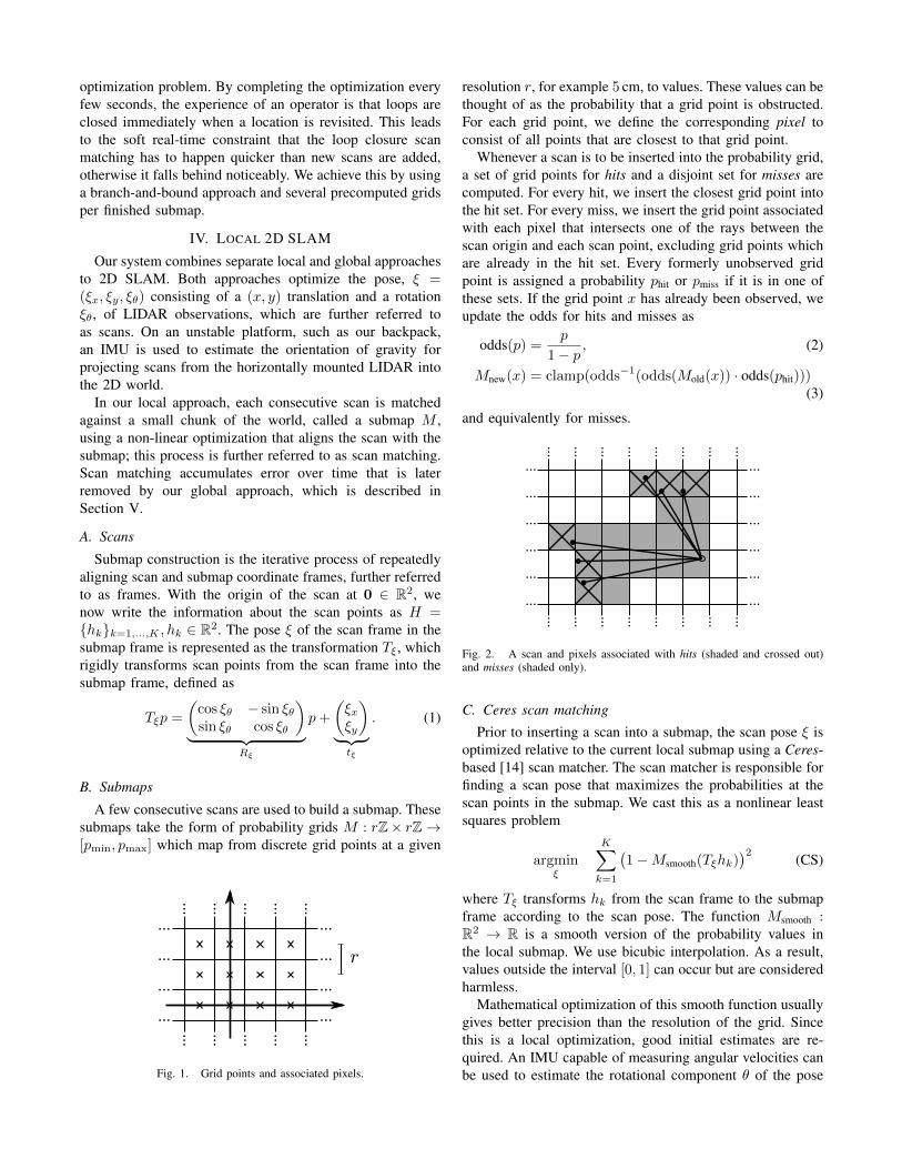
A few consecutive scans are used to build a submap. Thesesubmaps take the form of probability grids M : rZ× rZ→[pmin, pmax] which map from discrete grid points at a given

Fig. 1. Grid points and associated pixels.

resolution r, for example 5 cm, to values. These values can bethought of as the probability that a grid point is obstructed.For each grid point, we define the corresponding pixel toconsist of all points that are closest to that grid point.

Whenever a scan is to be inserted into the probability grid,a set of grid points for hits and a disjoint set for misses arecomputed. For every hit, we insert the closest grid point intothe hit set. For every miss, we insert the grid point associatedwith each pixel that intersects one of the rays between thescan origin and each scan point, excluding grid points whichare already in the hit set. Every formerly unobserved gridpoint is assigned a probability phit or pmiss if it is in one ofthese sets. If the grid point x has already been observed, weupdate the odds for hits and misses as

odds(p) =p

1− p, (2)

Mnew(x) = clamp(odds−1(odds(Mold(x)) · odds(phit)))(3)

and equivalently for misses.

Fig. 2. A scan and pixels associated with hits (shaded and crossed out)and misses (shaded only).

C. Ceres scan matching

Prior to inserting a scan into a submap, the scan pose ξ isoptimized relative to the current local submap using a Ceres-based [14] scan matcher. The scan matcher is responsible forfinding a scan pose that maximizes the probabilities at thescan points in the submap. We cast this as a nonlinear leastsquares problem

argminξ

K∑k=1

(1−Msmooth(Tξhk)

)2(CS)

where Tξ transforms hk from the scan frame to the submapframe according to the scan pose. The function Msmooth :R2 → R is a smooth version of the probability values inthe local submap. We use bicubic interpolation. As a result,values outside the interval [0, 1] can occur but are consideredharmless.

Mathematical optimization of this smooth function usuallygives better precision than the resolution of the grid. Sincethis is a local optimization, good initial estimates are re-quired. An IMU capable of measuring angular velocities canbe used to estimate the rotational component θ of the pose

between scan matches. A higher frequency of scan matchesor a pixel-accurate scan matching approach, although morecomputationally intensive, can be used in the absence of anIMU.

V. CLOSING LOOPS

As scans are only matched against a submap containinga few recent scans, the approach described above slowlyaccumulates error. For only a few dozen consecutive scans,the accumulated error is small.

Larger spaces are handled by creating many small sub-maps. Our approach, optimizing the poses of all scans andsubmaps, follows Sparse Pose Adjustment [2]. The relativeposes where scans are inserted are stored in memory for usein the loop closing optimization. In addition to these relativeposes, all other pairs consisting of a scan and a submapare considered for loop closing once the submap no longerchanges. A scan matcher is run in the background and ifa good match is found, the corresponding relative pose isadded to the optimization problem.

A. Optimization problem

Loop closure optimization, like scan matching, is alsoformulated as a nonlinear least squares problem which allowseasily adding residuals to take additional data into account.Once every few seconds, we use Ceres [14] to compute asolution to

argminΞm,Ξs

1

2

∑ij

ρ(E2(ξm

i , ξsj ; Σij , ξij)

)(SPA)

where the submap poses Ξm = {ξmi }i=1,...,m and the scan

poses Ξs = {ξsj}j=1,...,n in the world are optimized given

some constraints. These constraints take the form of relativeposes ξij and associated covariance matrices Σij . For a pairof submap i and scan j, the pose ξij describes where inthe submap coordinate frame the scan was matched. Thecovariance matrices Σij can be evaluated, for example, fol-lowing the approach in [15], or locally using the covarianceestimation feature of Ceres [14] with (CS). The residual Efor such a constraint is computed by

E2(ξmi , ξ

sj ; Σij , ξij) = e(ξm

i , ξsj ; ξij)

TΣ−1ij e(ξ

mi , ξ

sj ; ξij), (4)

e(ξmi , ξ

sj ; ξij) = ξij −

(R−1ξmi

(tξmi− tξs

j)

ξmi;θ − ξs

j;θ

). (5)

A loss function ρ, for example Huber loss, is used toreduce the influence of outliers which can appear in (SPA)when scan matching adds incorrect constraints to the opti-mization problem. For example, this may happen in locallysymmetric environments, such as office cubicles. Alternativeapproaches to outliers include [16].

B. Branch-and-bound scan matching

We are interested in the optimal, pixel-accurate match

ξ? = argmaxξ∈W

K∑k=1

Mnearest(Tξhk), (BBS)

where W is the search window and Mnearest is M extendedto all of R2 by rounding its arguments to the nearest gridpoint first, that is extending the value of a grid points tothe corresponding pixel. The quality of the match can beimproved further using (CS).

Efficiency is improved by carefully choosing step sizes.We choose the angular step size δθ so that scan points at themaximum range dmax do not move more than r, the widthof one pixel. Using the law of cosines, we derive

dmax = maxk=1,...,K

‖hk‖, (6)

δθ = arccos(1− r2

2d2max

). (7)

We compute an integral number of steps covering givenlinear and angular search window sizes, e.g., Wx = Wy =7 m and Wθ = 30◦,

wx =

⌈Wx

r

⌉, wy =

⌈Wy

r

⌉, wθ =

⌈Wθ

δθ

⌉. (8)

This leads to a finite set W forming a search windowaround an estimate ξ0 placed in its center,

W = {−wx, . . . , wx} × {−wy, . . . , wy} × {−wθ, . . . , wθ},(9)

W = {ξ0 + (rjx, rjy, δθjθ) : (jx, jy, jθ) ∈ W}. (10)

A naive algorithm to find ξ? can easily be formulated, seeAlgorithm 1, but for the search window sizes we have inmind it would be far too slow.

Algorithm 1 Naive algorithm for (BBS)best score← −∞for jx = −wx to wx do

for jy = −wy to wy dofor jθ = −wθ to wθ doscore←

∑Kk=1Mnearest(Tξ0+(rjx,rjy,δθjθ)hk)

if score > best score thenmatch← ξ0 + (rjx, rjy, δθjθ)best score← score

end ifend for

end forend forreturn best score and match when set.

Instead, we use a branch and bound approach to efficientlycompute ξ? over larger search windows. See Algorithm 2 forthe generic approach. This approach was first suggested inthe context of mixed integer linear programs [17]. Literatureon the topic is extensive; see [18] for a short overview.

The main idea is to represent subsets of possibilities asnodes in a tree where the root node represents all possiblesolutions, W in our case. The children of each node form apartition of their parent, so that they together represent thesame set of possibilities. The leaf nodes are singletons; eachrepresents a single feasible solution. Note that the algorithmis exact. It provides the same solution as the naive approach,

as long as the score(c) of inner nodes c is an upper boundon the score of its elements. In that case, whenever a nodeis bounded, a solution better than the best known solutionso far does not exist in this subtree.

To arrive at a concrete algorithm, we have to decide onthe method of node selection, branching, and computationof upper bounds.

1) Node selection: Our algorithm uses depth-first search(DFS) as the default choice in the absence of a betteralternative: The efficiency of the algorithm depends on alarge part of the tree being pruned. This depends on twothings: a good upper bound, and a good current solution. Thelatter part is helped by DFS, which quickly evaluates manyleaf nodes. Since we do not want to add poor matches asloop closing constraints, we also introduce a score thresholdbelow which we are not interested in the optimal solution.Since in practice the threshold will not often be surpassed,this reduces the importance of the node selection or findingan initial heuristic solution. Regarding the order in whichthe children are visited during the DFS, we compute theupper bound on the score for each child, visiting the mostpromising child node with the largest bound first. Thismethod is Algorithm 3.

2) Branching rule: Each node in the tree is described bya tuple of integers c = (cx, cy, cθ, ch) ∈ Z4. Nodes at heightch combine up to 2ch×2ch possible translations but representa specific rotation:

Wc =

({(jx, jy) ∈ Z2 : (11)

cx ≤ jx < cx + 2ch

cy ≤ jy < cy + 2ch

}× {cθ}

),

Wc =Wc ∩W. (12)

Algorithm 2 Generic branch and boundbest score← −∞C ← C0while C 6= ∅ do

Select a node c ∈ C and remove it from the set.if c is a leaf node then

if score(c) > best score thensolution← nbest score← score(c)

end ifelse

if score(c) > best score thenBranch: Split c into nodes Cc.C ← C ∪ Cc

elseBound.

end ifend if

end whilereturn best score and solution when set.

Algorithm 3 DFS branch and bound scan matcher for (BBS)best score← score thresholdCompute and memorize a score for each element in C0.Initialize a stack C with C0 sorted by score, the maximumscore at the top.while C is not empty do

Pop c from the stack C.if score(c) > best score then

if c is a leaf node thenmatch← ξcbest score← score(c)

elseBranch: Split c into nodes Cc.Compute and memorize a score for each elementin Cc.Push Cc onto the stack C, sorted by score, themaximum score last.

end ifend if

end whilereturn best score and match when set.

Leaf nodes have height ch = 0, and correspond to feasiblesolutions W 3 ξc = ξ0 + (rcx, rcy, δθcθ).

In our formulation of Algorithm 3, the root node, encom-passing all feasible solutions, does not explicitly appear andbranches into a set of initial nodes C0 at a fixed height h0

covering the search window

W0,x = {−wx + 2h0jx : jx ∈ Z, 0 ≤ 2h0jx ≤ 2wx},W0,y = {−wy + 2h0jy : jy ∈ Z, 0 ≤ 2h0jy ≤ 2wy},W0,θ = {jθ ∈ Z : −wθ ≤ jθ ≤ wθ},C0 =W0,x ×W0,y ×W0,θ × {h0}.

(13)

At a given node c with ch > 1, we branch into up to fourchildren of height ch − 1

Cc =(({cx, cx + 2ch−1} × {cy, cy + 2ch−1}

× cθ)∩W

)× {ch − 1}.

(14)

3) Computing upper bounds: The remaining part of thebranch and bound approach is an efficient way to computeupper bounds at inner nodes, both in terms of computationaleffort and in the quality of the bound. We use

score(c) =

K∑k=1

maxj∈Wc

Mnearest(Tξjhk)

≥K∑k=1

maxj∈Wc

Mnearest(Tξjhk)

≥ maxj∈Wc

K∑k=1

Mnearest(Tξjhk).

(15)

To be able to compute the maximum efficiently, we useprecomputed grids M ch

precomp. Precomputing one grid perpossible height ch allows us to compute the score with effort

linear in the number of scan points. Note that, to be able todo this, we also compute the maximum over Wc which canbe larger than Wc near the boundary of our search space.

score(c) =

K∑k=1

M chprecomp(Tξchk), (16)

Mhprecomp(x, y) = max

x′∈[x,x+r(2h−1)]

y′∈[y,y+r(2h−1)]

Mnearest(x′, y′) (17)

with ξc as before for the leaf nodes. Note that Mhprecomp has

the same pixel structure as Mnearest, but in each pixel storingthe maximum of the values of the 2h × 2h box of pixelsbeginning there. An example of such precomputed grids isgiven in Figure 3.

Fig. 3. Precomputed grids of size 1, 4, 16 and 64.

To keep the computational effort for constructing theprecomputed grids low, we wait until a probability grid willreceive no further updates. Then we compute a collection ofprecomputed grids, and start matching against it.

For each precomputed grid, we compute the maximum ofa 2h pixel wide row starting at each pixel. Using this inter-mediate result, the next precomputed grid is then constructed.

The maximum of a changing collection of values can bekept up-to-date in amortized O(1) if values are removedin the order in which they have been added. Successivemaxima are kept in a deque that can be defined recursivelyas containing the maximum of all values currently in thecollection followed by the list of successive maxima of allvalues after the first occurrence of the maximum. For anempty collection of values, this list is empty. Using thisapproach, the precomputed grids can be computed in O(n)where n is the number of pixels in each precomputed grids.

An alternative way to compute upper bounds is to computelower resolution probability grids, successively halving theresolution, see [1]. Since the additional memory consumptionof our approach is acceptable, we prefer it over using lowerresolution probability grids which lead to worse bounds than(15) and thus negatively impact performance.

VI. EXPERIMENTAL RESULTS

In this section, we present some results of our SLAM al-gorithm computed from recorded sensor data using the sameonline algorithms that are used interactively on the backpack.First, we show results using data collected by the sensors

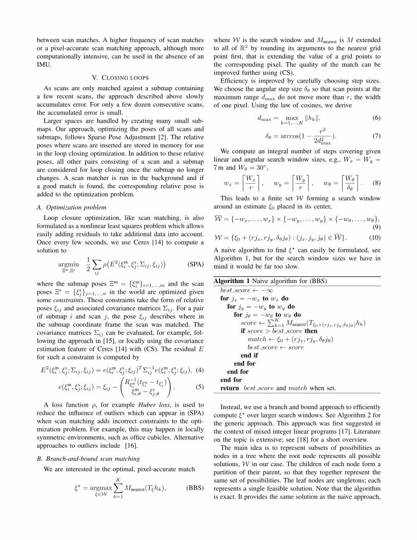
Fig. 4. Cartographer map of the 2nd floor of the Deutsches Museum.

of our Cartographer backpack in the Deutsches Museum inMunich. Second, we demonstrate that our algorithms workwell with inexpensive hardware by using data collected froma robotic vacuum cleaner sensor. Lastly, we show resultsusing the Radish data set [19] and compare ourselves topublished results.

A. Real-World Experiment: Deutsches Museum

Using data collected at the Deutsches Museum spanning1,913 s of sensor data or 2,253 m (according to the computedsolution), we computed the map shown in Figure 4. Ona workstation with an Intel Xeon E5-1650 at 3.2 GHz,our SLAM algorithm uses 1,018 s CPU time, using up to2.2 GB of memory and up to 4 background threads for loopclosure scan matching. It finishes after 360 s wall clock time,meaning it achieved 5.3 times real-time performance.

The generated graph for the loop closure optimizationconsists of 11,456 nodes and 35,300 edges. The optimizationproblem (SPA) is run every time a few nodes have beenadded to the graph. A typical solution takes about 3 itera-tions, and finishes in about 0.3 s.

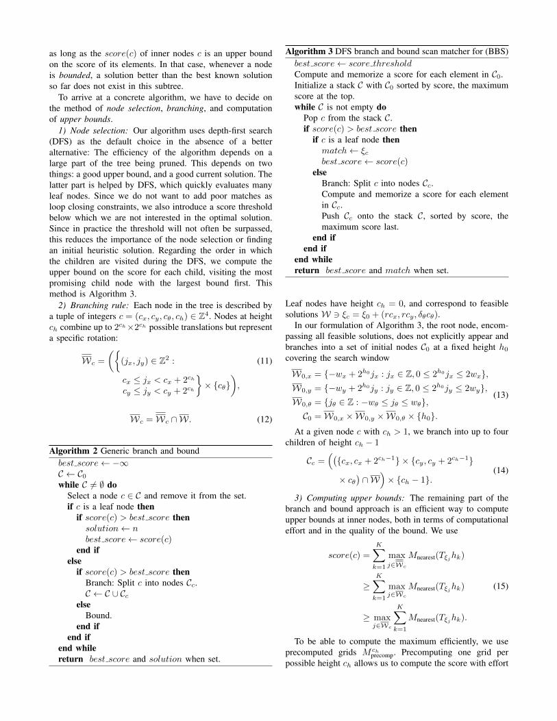
Fig. 5. Cartographer map generated using Revo LDS sensor data.

TABLE IQUANTITATIVE ERRORS WITH REVO LDS

Laser Tape Cartographer Error (absolute) Error (relative)

4.09 4.08 −0.01 −0.2%5.40 5.43 +0.03 +0.6%8.67 8.74 +0.07 +0.8%15.09 15.20 +0.11 +0.7%15.12 15.23 +0.11 +0.7%

B. Real-World Experiment: Neato’s Revo LDS

Neato Robotics uses a laser distance sensor (LDS) calledRevo LDS [20] in their vacuum cleaners which costs under$ 30. We captured data by pushing around the vacuumcleaner on a trolley while taking scans at approximately 2 Hzover its debug connection. Figure 5 shows the resulting 5 cmresolution floor plan. To evaluate the quality of the floor plan,we compare laser tape measurements for 5 straight lines tothe pixel distance in the resulting map as computed by adrawing tool. The results are presented in Table I, all valuesare in meters. The values are roughly in the expected orderof magnitude of one pixel at each end of the line.

C. Comparisons using the Radish data set

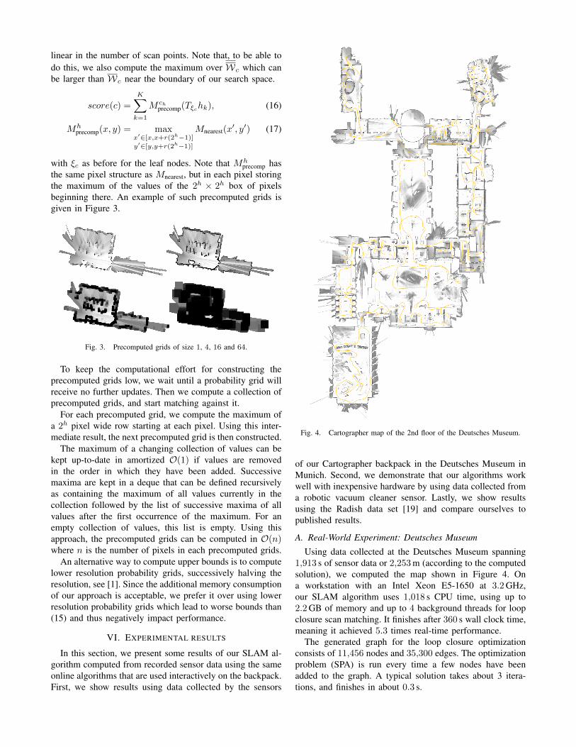
We compare our approach to others using the benchmarkmeasure suggested in [21], which compares the error in rela-tive pose changes to manually curated ground truth relations.Table II shows the results computed by our CartographerSLAM algorithm. For comparison, we quote results forGraph Mapping (GM) from [21]. Additionally, we quotemore recently published results from [9] in Table III. Allerrors are given in meters and degrees, either absolute orsquared, together with their standard deviation.

Each public data set was collected with a unique sensorconfiguration that differs from our Cartographer backpack.Therefore, various algorithmic parameters needed to beadapted to produce reasonable results. In our experience, tun-ing Cartographer is only required to match the algorithm tothe sensor configuration and not to the specific surroundings.

TABLE IIQUANTITATIVE COMPARISON OF ERROR WITH [21]

Cartographer GM

AcesAbsolute translational 0.0375± 0.0426 0.044± 0.044Squared translational 0.0032± 0.0285 0.004± 0.009Absolute rotational 0.373± 0.469 0.4± 0.4Squared rotational 0.359± 3.696 0.3± 0.8

IntelAbsolute translational 0.0229± 0.0239 0.031± 0.026Squared translational 0.0011± 0.0040 0.002± 0.004Absolute rotational 0.453± 1.335 1.3± 4.7Squared rotational 1.986± 23.988 24.0± 166.1

MIT Killian CourtAbsolute translational 0.0395± 0.0488 0.050± 0.056Squared translational 0.0039± 0.0144 0.006± 0.029Absolute rotational 0.352± 0.353 0.5± 0.5Squared rotational 0.248± 0.610 0.9± 0.9

MIT CSAILAbsolute translational 0.0319± 0.0363 0.004± 0.009Squared translational 0.0023± 0.0099 0.0001± 0.0005Absolute rotational 0.369± 0.365 0.05± 0.08Squared rotational 0.270± 0.637 0.01± 0.04

Freiburg bldg 79Absolute translational 0.0452± 0.0354 0.056± 0.042Squared translational 0.0033± 0.0055 0.005± 0.011Absolute rotational 0.538± 0.718 0.6± 0.6Squared rotational 0.804± 3.627 0.7± 1.7

Freiburg hospital (local)Absolute translational 0.1078± 0.1943 0.143± 0.180Squared translational 0.0494± 0.2831 0.053± 0.272Absolute rotational 0.747± 2.047 0.9± 2.2Squared rotational 4.745± 40.081 5.5± 46.2

Freiburg hospital (global)Absolute translational 5.2242± 6.6230 11.6± 11.9Squared translational 71.0288± 267.7715 276.1± 516.5Absolute rotational 3.341± 4.797 6.3± 6.2Squared rotational 34.107± 127.227 77.2± 154.8

Since each public data set has a unique sensor config-uration, we cannot be sure that we did not also fit ourparameters to the specific locations. The only exception beingthe Freiburg hospital data set where there are two separaterelations files. We tuned our parameters using the localrelations but also see good results on the global relations.

TABLE IIIQUANTITATIVE COMPARISON OF ERROR WITH [9]

Cartographer Graph FLIRT

IntelAbsolute translational 0.0229± 0.0239 0.02± 0.02Absolute rotational 0.453± 1.335 0.3± 0.3

Freiburg bldg 79Absolute translational 0.0452± 0.0354 0.06± 0.09Absolute rotational 0.538± 0.718 0.8± 1.1

Freiburg hospital (local)Absolute translational 0.1078± 0.1943 0.18± 0.27Absolute rotational 0.747± 2.047 0.9± 2.0

Freiburg hospital (global)Absolute translational 5.2242± 6.6230 8.3± 8.6Absolute rotational 3.341± 4.797 5.0± 5.3

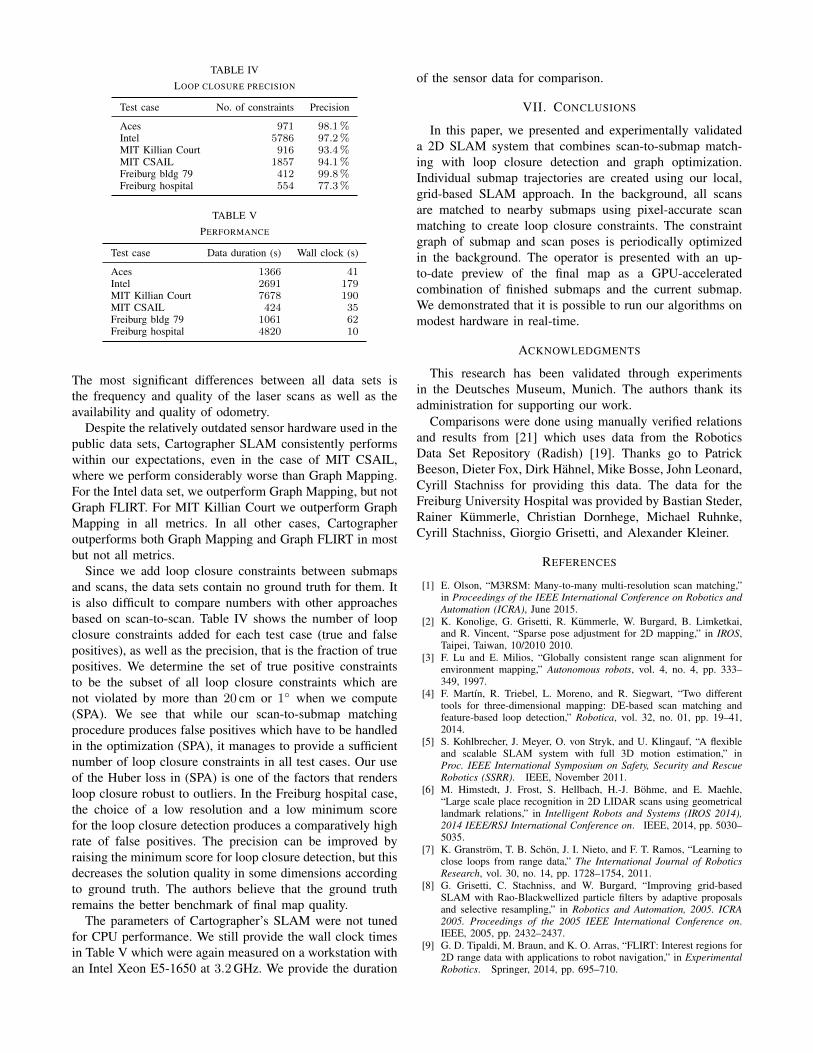
TABLE IVLOOP CLOSURE PRECISION

Test case No. of constraints Precision

Aces 971 98.1%Intel 5786 97.2%MIT Killian Court 916 93.4%MIT CSAIL 1857 94.1%Freiburg bldg 79 412 99.8%Freiburg hospital 554 77.3%

TABLE VPERFORMANCE

Test case Data duration (s) Wall clock (s)

Aces 1366 41Intel 2691 179MIT Killian Court 7678 190MIT CSAIL 424 35Freiburg bldg 79 1061 62Freiburg hospital 4820 10

The most significant differences between all data sets isthe frequency and quality of the laser scans as well as theavailability and quality of odometry.

Despite the relatively outdated sensor hardware used in thepublic data sets, Cartographer SLAM consistently performswithin our expectations, even in the case of MIT CSAIL,where we perform considerably worse than Graph Mapping.For the Intel data set, we outperform Graph Mapping, but notGraph FLIRT. For MIT Killian Court we outperform GraphMapping in all metrics. In all other cases, Cartographeroutperforms both Graph Mapping and Graph FLIRT in mostbut not all metrics.

Since we add loop closure constraints between submapsand scans, the data sets contain no ground truth for them. Itis also difficult to compare numbers with other approachesbased on scan-to-scan. Table IV shows the number of loopclosure constraints added for each test case (true and falsepositives), as well as the precision, that is the fraction of truepositives. We determine the set of true positive constraintsto be the subset of all loop closure constraints which arenot violated by more than 20 cm or 1◦ when we compute(SPA). We see that while our scan-to-submap matchingprocedure produces false positives which have to be handledin the optimization (SPA), it manages to provide a sufficientnumber of loop closure constraints in all test cases. Our useof the Huber loss in (SPA) is one of the factors that rendersloop closure robust to outliers. In the Freiburg hospital case,the choice of a low resolution and a low minimum scorefor the loop closure detection produces a comparatively highrate of false positives. The precision can be improved byraising the minimum score for loop closure detection, but thisdecreases the solution quality in some dimensions accordingto ground truth. The authors believe that the ground truthremains the better benchmark of final map quality.

The parameters of Cartographer’s SLAM were not tunedfor CPU performance. We still provide the wall clock timesin Table V which were again measured on a workstation withan Intel Xeon E5-1650 at 3.2 GHz. We provide the duration

of the sensor data for comparison.

VII. CONCLUSIONS

In this paper, we presented and experimentally validateda 2D SLAM system that combines scan-to-submap match-ing with loop closure detection and graph optimization.Individual submap trajectories are created using our local,grid-based SLAM approach. In the background, all scansare matched to nearby submaps using pixel-accurate scanmatching to create loop closure constraints. The constraintgraph of submap and scan poses is periodically optimizedin the background. The operator is presented with an up-to-date preview of the final map as a GPU-acceleratedcombination of finished submaps and the current submap.We demonstrated that it is possible to run our algorithms onmodest hardware in real-time.

ACKNOWLEDGMENTS

This research has been validated through experimentsin the Deutsches Museum, Munich. The authors thank itsadministration for supporting our work.

Comparisons were done using manually verified relationsand results from [21] which uses data from the RoboticsData Set Repository (Radish) [19]. Thanks go to PatrickBeeson, Dieter Fox, Dirk Hahnel, Mike Bosse, John Leonard,Cyrill Stachniss for providing this data. The data for theFreiburg University Hospital was provided by Bastian Steder,Rainer Kummerle, Christian Dornhege, Michael Ruhnke,Cyrill Stachniss, Giorgio Grisetti, and Alexander Kleiner.

REFERENCES

[1] E. Olson, “M3RSM: Many-to-many multi-resolution scan matching,”in Proceedings of the IEEE International Conference on Robotics andAutomation (ICRA), June 2015.

[2] K. Konolige, G. Grisetti, R. Kummerle, W. Burgard, B. Limketkai,and R. Vincent, “Sparse pose adjustment for 2D mapping,” in IROS,Taipei, Taiwan, 10/2010 2010.

[3] F. Lu and E. Milios, “Globally consistent range scan alignment forenvironment mapping,” Autonomous robots, vol. 4, no. 4, pp. 333–349, 1997.

[4] F. Martın, R. Triebel, L. Moreno, and R. Siegwart, “Two differenttools for three-dimensional mapping: DE-based scan matching andfeature-based loop detection,” Robotica, vol. 32, no. 01, pp. 19–41,2014.

[5] S. Kohlbrecher, J. Meyer, O. von Stryk, and U. Klingauf, “A flexibleand scalable SLAM system with full 3D motion estimation,” inProc. IEEE International Symposium on Safety, Security and RescueRobotics (SSRR). IEEE, November 2011.

[6] M. Himstedt, J. Frost, S. Hellbach, H.-J. Bohme, and E. Maehle,“Large scale place recognition in 2D LIDAR scans using geometricallandmark relations,” in Intelligent Robots and Systems (IROS 2014),2014 IEEE/RSJ International Conference on. IEEE, 2014, pp. 5030–5035.

[7] K. Granstrom, T. B. Schon, J. I. Nieto, and F. T. Ramos, “Learning toclose loops from range data,” The International Journal of RoboticsResearch, vol. 30, no. 14, pp. 1728–1754, 2011.

[8] G. Grisetti, C. Stachniss, and W. Burgard, “Improving grid-basedSLAM with Rao-Blackwellized particle filters by adaptive proposalsand selective resampling,” in Robotics and Automation, 2005. ICRA2005. Proceedings of the 2005 IEEE International Conference on.IEEE, 2005, pp. 2432–2437.

[9] G. D. Tipaldi, M. Braun, and K. O. Arras, “FLIRT: Interest regions for2D range data with applications to robot navigation,” in ExperimentalRobotics. Springer, 2014, pp. 695–710.

[10] J. Strom and E. Olson, “Occupancy grid rasterization in large environ-ments for teams of robots,” in Intelligent Robots and Systems (IROS),2011 IEEE/RSJ International Conference on. IEEE, 2011, pp. 4271–4276.

[11] R. Kummerle, G. Grisetti, H. Strasdat, K. Konolige, and W. Burgard,“g2o: A general framework for graph optimization,” in Robotics andAutomation (ICRA), 2011 IEEE International Conference on. IEEE,2011, pp. 3607–3613.

[12] L. Carlone, R. Aragues, J. A. Castellanos, and B. Bona, “A fastand accurate approximation for planar pose graph optimization,” TheInternational Journal of Robotics Research, pp. 965–987, 2014.

[13] M. Bosse and R. Zlot, “Map matching and data association for large-scale two-dimensional laser scan-based SLAM,” The InternationalJournal of Robotics Research, vol. 27, no. 6, pp. 667–691, 2008.

[14] S. Agarwal, K. Mierle, and Others, “Ceres solver,” http://ceres-solver.org.

[15] E. B. Olson, “Real-time correlative scan matching,” in Roboticsand Automation, 2009. ICRA’09. IEEE International Conference on.IEEE, 2009, pp. 4387–4393.

[16] P. Agarwal, G. D. Tipaldi, L. Spinello, C. Stachniss, and W. Burgard,“Robust map optimization using dynamic covariance scaling,” inRobotics and Automation (ICRA), 2013 IEEE International Conferenceon. IEEE, 2013, pp. 62–69.

[17] A. H. Land and A. G. Doig, “An automatic method of solving discreteprogramming problems,” Econometrica, vol. 28, no. 3, pp. 497–520,1960.

[18] J. Clausen, “Branch and bound algorithms-principles and examples,”Department of Computer Science, University of Copenhagen, pp. 1–30, 1999.

[19] A. Howard and N. Roy, “The robotics data set repository (Radish),”2003. [Online]. Available: http://radish.sourceforge.net/

[20] K. Konolige, J. Augenbraun, N. Donaldson, C. Fiebig, and P. Shah,“A low-cost laser distance sensor,” in Robotics and Automation, 2008.ICRA 2008. IEEE International Conference on. IEEE, 2008, pp.3002–3008.

[21] R. Kummerle, B. Steder, C. Dornhege, M. Ruhnke, G. Grisetti,C. Stachniss, and A. Kleiner, “On measuring the accuracy of SLAMalgorithms,” Autonomous Robots, vol. 27, no. 4, pp. 387–407, 2009.