Embed Size (px)
Citation preview
Technical report, IDE0743 , December 2, 2007
On Stock Index Volatility WithRespect to Capitalization
Master’s Thesis in Financial Mathematics
Anna Bronskaya and Marina Pachentseva
School of Information Science, Computer and Electrical EngineeringHalmstad University

On Stock Index Volatility WithRespect to Capitalization
Anna Bronskaya and Marina Pachentseva
Halmstad University
Project Report IDE0743
Master’s thesis in Financial Mathematics, 15 ECTS credits
Supervisor: Ph.D. Jan-Olof JohanssonExaminer: Prof. Ljudmila A. Bordag
External refrees: Prof. Krzysztof Szajowski
December 2, 2007
Department of Mathematics, Physics and Electrical engineeringSchool of Information Science, Computer and Electrical Engineering
Halmstad University

Preface
First we would like to thank our supervisor and examiner Ph.D. Jan-OlofJohansson and Prof. Ljudmila A. Bordag for the opportunity to write ourmaster thesis at Halmstad University. We further want to express the grati-tude to professor Shyriaev Albert Nikolaevich and professor Mikhail Nechaevfor their support and suggestions. We would also like to thank the staff ofDepartment of Mathematics, Physics and Electrical engineering School ofInformation Science, Computer and Electrical Engineering for making thegreat stay at University.
Halmstad, May 2007Anna Bronskaya, Marina Pachentseva

ii
Abstract
Confidence in the future is a significant factor for business develop-ment.However frequently, accurate and specific purposes are spread overthe market environment influence. Thus, it is necessary to make an ap-propriate consideration of instability, which is peculiar to the dynamicdevelopment. Volatility, variance and standard deviation are used tocharacterize the deviation of the investigated quantity from mean value.Volatility is one of the main instruments to measure the risk of the asset.The increasing availability of financial market data has enlarged volatil-ity research potential but has also encouraged research into longer hori-zon volatility forecasts. In this paper we investigate stock index volatilitywith respect to capitalization with help of GARCH-modelling.There are chosen three indexes of OMX Nordic Exchange for our re-search. The Nordic list segment indexes comprising Nordic Large Cap,Mid Cap and Small Cap are based on the three market capitalizationgroups.We implement GARCH-modeling for considering indexes and compareour results in order to conclude which ones of the indexes is more volatile.The OMX Nordic list index is quiet new (2002) and reorganized as lateas October 2006. The current value is now about 300 and no options doexist. In current work we are also interested in estimation of the Hestonmodel (SV model), which is popular in financial world and can be usedin option pricing in the future.The results of our investigations show that Large Cap Index is morevolatile then Middle and Small Cap Indexes.Keywords: GARCH models, volatility, Heston Model.
iii

iv
Contents
1 Introduction 11.1 Background . . . . . . . . . . . . . . . . . . . . . . . . . . . . 11.2 Limitations . . . . . . . . . . . . . . . . . . . . . . . . . . . . 11.3 Readers guide . . . . . . . . . . . . . . . . . . . . . . . . . . . 1
2 Volatility 32.1 Historical Volatility . . . . . . . . . . . . . . . . . . . . . . . . 32.2 ARCH/GARCH models . . . . . . . . . . . . . . . . . . . . . 42.3 Implied Volatility . . . . . . . . . . . . . . . . . . . . . . . . . 62.4 Stochastic volatility . . . . . . . . . . . . . . . . . . . . . . . . 7
3 Index Return Data and Volatility 93.1 Data and Statistical analysis . . . . . . . . . . . . . . . . . . . 9
4 Theory 154.1 Statistics . . . . . . . . . . . . . . . . . . . . . . . . . . . . . . 154.2 Hypothesis tests . . . . . . . . . . . . . . . . . . . . . . . . . . 164.3 ARCH - Autoregressive conditional heteroskedasticity . . . . . 174.4 Generalized ARCH - GARCH . . . . . . . . . . . . . . . . . . 18
5 GARCH Model and Estimations 215.1 Daily GARCH (1, 1)-model . . . . . . . . . . . . . . . . . . . 215.2 Estimation . . . . . . . . . . . . . . . . . . . . . . . . . . . . . 215.3 Forecasting of the volatility using historical data . . . . . . . . 23
5.3.1 Volatility prediction . . . . . . . . . . . . . . . . . . . 255.3.2 Forecasting of 10-days - ahead volatility . . . . . . . . 275.3.3 Results . . . . . . . . . . . . . . . . . . . . . . . . . . . 29
6 Validation of the Heston Model 316.1 The Heston Model . . . . . . . . . . . . . . . . . . . . . . . . 316.2 Estimation and testing model . . . . . . . . . . . . . . . . . . 32
v
6.3 Simulated results . . . . . . . . . . . . . . . . . . . . . . . . . 346.4 GARCH simulations of the ”Heston process” . . . . . . . . . . 376.5 Calibration of the model . . . . . . . . . . . . . . . . . . . . . 39
7 Conclusions 41
Bibliography 43
Appendix 45
vi
Chapter 1
Introduction
1.1 Background
Measuring the risk on specific assets has become important during the lastyears due to the growth of financial markets. Companies want to have acontrol of their risk portfolios. Risk can be divided into different categories:strategic risk, operational risk and financial risks. One of risk measure isvolatility. In this thesis we focus on stock indices. Calculating volatility isimportant in pricing derivatives, portfolio selection and hedging strategies.
1.2 Limitations
To give trustworthy results it is necessary to limit the problem. In this thesiswe focus on univariate volatility modeling. The multivariate case is notconcerned. We are working with daily data and are interested in one-step-ahead volatility prediction. The model chosen for investigation is GARCHmodel. We also selected Heston Model for volatility estimation due to furtherdevelopments of chosen indices.
1.3 Readers guide
Each chapter is briefly presented below.
Chapter 1 is the introduction chapter. It presents the thesis.
Chapter 2 is about existent volatility types.
Chapter 3 is about market data set which is used in the thesis.
1
2 Chapter 1. Introduction
Chapter 4 represents the theory has been used in the researches.
Chapter 5 is about model used for investigations. Here the GARCH model,estimation procedure, prediction and toolboxes are presented.
Chapter 6 is the chapter about Heston model and its estimation.
It is supposed that the reader has knowledge on stochastic processes andprobability theory. General knowledge about stock market is also assumed.
Chapter 2
Volatility
Volatility is one of the main instruments to measure the risk of asset. Thereare great number of volatility models which are used by traders, financialanalytics and risk managers. Below we describe some of them and also discusspossibilities in their using for trading and risk measure.
2.1 Historical Volatility
The absence of volatility calculations in numerous reports and reviews oftechnical analytics is connected mostly with useless of this idea for majorityof active traders working during the day.
Simple volatility σ is a standard deviation of returns St of the asset duringN traded periods, [3]:
σ =
√∑t
(ht − h)2
N − 1, (2.1)
where
ht = ln( St
St−1) - ”logarithmic returns”,
St - closing price for time interval i.
Usually, one day period is used as a time interval and it is denoted dailyvolatility. If hour is taken as a time interval, then such volatility is calledhour volatility and so forth.
Daily volatility calculated with (2.1) is called active historical volatility.Active means that volatility is calculated by the present moment and his-torical means that volatility is calculated with already realized sampling ofhistorical data.
3
4 Chapter 2. Volatility
The most important in those definitions is the value of sampling N . De-pending on a value of N and a concrete sampling of time series h, we canobtain σ values which differ from each other two - three times or more. Firstof all it is connected with a fact that the mean value of return h (whichdetermine active trend) has strong dependence on the size and condition ofsampling in the past. And secondly, different phases of market activity givedifferent standard deviation of returns. The value of h(N) for big size ofsampling N will define medium-term and long-term trends, and for smallsize of sampling N will define correspondingly short-term dynamics of quo-tations. These trends can have different signs and, that is more essential,can be changed in time. That is why the active average yield h and activevolatility are dissimilar and have to be different from corresponding valuestwo months ago, and also from those that will be realized in a month.
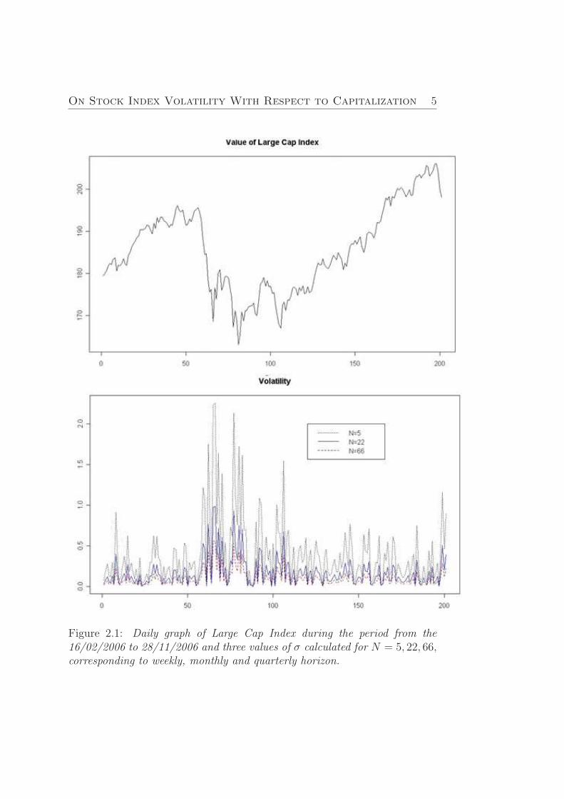
In the Figure (2.1) is represented a graph of Large Cap Index quotationsand values of historical volatility. The values of volatility are calculated withhelp of the statistical R package.
Figure shows us that volatility strongly depends on values of sampling Nand on market stage. Volatility which is calculated on the base on short-termaveraging is the most unstable. It is also obvious that short-term volatility isheavily clusterized. And at the same time the scale of the cluster is coincidewith the value of sampling N . But this effect has a certain attitude toward themethod to define the volatility (2.1), where all traded periods are includedwith the same weights, what is a disadvantage of this method of volatilitycalculation. In connection with such issues there are exist different ways todefine volatility.
2.2 ARCH/GARCH models
On Stock Index Volatility With Respect to Capitalization 5
Figure 2.1: Daily graph of Large Cap Index during the period from the16/02/2006 to 28/11/2006 and three values of σ calculated for N = 5, 22, 66,corresponding to weekly, monthly and quarterly horizon.
6 Chapter 2. Volatility
GARCH methods are used to construct the function of past returns andon the base on that function see future movements of financial time series.This is an approach that will be used in this work and will be explainedfurther.
The main method of using volatility, as was noticed above, is to determinelimits for possible values of return hn+1 on the next step n + 1. That is whythe trader tries to use volatility for quiet short forecast (one day or threeforward), then, first of all, he can reduce size of sampling N up to minimalreasonable level (in order to exclude influence of earlier data). However,the reliability of determination of σ value is falling by that. And, secondly,trader can use autoregressive and heteroskedasticity models for volatility(ARCH, GARCH, etc.). These models allow taking into account the effectof ”clusterization” on the market (periods on market when absolute valuesof volatility take big or small values). The effect of ”clusterization” can beseen on Figure (2.1).
2.3 Implied Volatility
Implied volatility coincides with option pricing. The most popular and well-developed model for option pricing is the Black-Scholes Model, which hasfollowing formulation for call option:
C(S, T ) = SN(d+)−KerT N(d−), (2.2)
where
d± =ln( S
K)+(r±0.5σ2)T
σ√
T
K - exercise price;
S - strike price;
r - interest rate;
σ - constant volatility;
N(x) - standard normal distribution function;
T - expire date.
The key assumptions of the Black-Scholes model are:
On Stock Index Volatility With Respect to Capitalization 7
• The price of the underlying instrument St follows a geometric Brownianmotion with constant drift µ and volatility σ:
dSt = µStdt + σStdWt, where dWt is a geometrical Brownian motion;
• It is possible to short sell the underlying stock.
• There are no arbitrage opportunities.
• Trading in the stock is continuous.
• There are no transaction costs or taxes.
• All securities are perfectly divisible.
• It is possible to borrow and lend cash at a constant risk-free interestrate.
There are many different variations of the Black-Scholes model which cor-rect these assumptions. Option pricing models help to evaluate the problem:what is the price of a concrete option at the present time. But very oftenthe fair price and real price are different. As a result of this it is said aboutimplied volatility, which can be calculated, with help of numerical methods,by substitution all know parameters into the Black-Scholes Model. Thus, itmakes sense to talk about volatility when there are derivatives on underlyingasset.
2.4 Stochastic volatility
Options on the same underlier but with different strike price and expiredate have different implied volatility. Thus, volatility of an underlier is notconstant, but depends on different factors such as price, variance and we cantalk about stochastic volatility models, which are used in financial world. Themain value in stochastic volatility models is a correlation between price modeland volatility model, which is denoted by ρ. The evaluation of stochasticvolatility models was started by Hull and White ( ρ = 0, 1987) and Wiggins( ρ 6= 0, 1987), when they introduced following model:
dσ
σ= µdt + ξdW, (2.3)
where the volatility is an exponential Brownian motion.Scott (ρ 6= 0, 1989) considered the case in which the logarithm of the
volatility is an Ornstein-Uhlenbeck (OU) process or a Gauss-Markov process.
8 Chapter 2. Volatility
dln(σ2) = (w − ζln(σ2))dt + ξdW. (2.4)
These two models have the advantage that the volatility is positive allthe time. The model proposed by Scott (1987) was further investigated byStein and Stein (ρ = 0, 1991). They considered volatility itself as an OUprocess.
dσ = (w − ζσ)dt + ξdW. (2.5)
The disadvantage of this model is that the volatility can become negative.The final model was proposed by Heston (ρ 6= 0, 1993).
dσ = (w − ζσ2)dt + ξσdW2. (2.6)
For small dt, this model keeps the volatility positive and is the mostpopular model because it allows the correlation between asset returns andvolatility.
In spite of the fact that continuous time models provide the natural struc-ture for an analysis of option pricing, discrete time models (such as ARCH,GARCH models) are ideal for the statistical analysis of daily price changes,which we have deal with un current paper.
In this paper we examine GARCH model on daily price changes of NordicList Segment Indexes in order to investigate which of indexes is more volatileand to forecast future volatility. Also in current work made an attempt tosimulate Heston model corresponding to changes of Large Cap Index.
Chapter 3
Index Return Data andVolatility
3.1 Data and Statistical analysis
The data for our research consists of OMX Large Cap (Middle Cap, SmallCap) Index (see Appendix A) closing prices during the period 30th December2002 to 8th May 2007.
Let us denote closing prices for n days by S = {St}t=1..n , n = 1110.Taking into the account further studying of stochastic indexes component, itis better to work with quantities ht = ln( St
St−1), (t = 1...n) instead of prices
itself S = {St}t=1..n. These quantities are usually denoted logarithmic returnsand are used in volatility models.
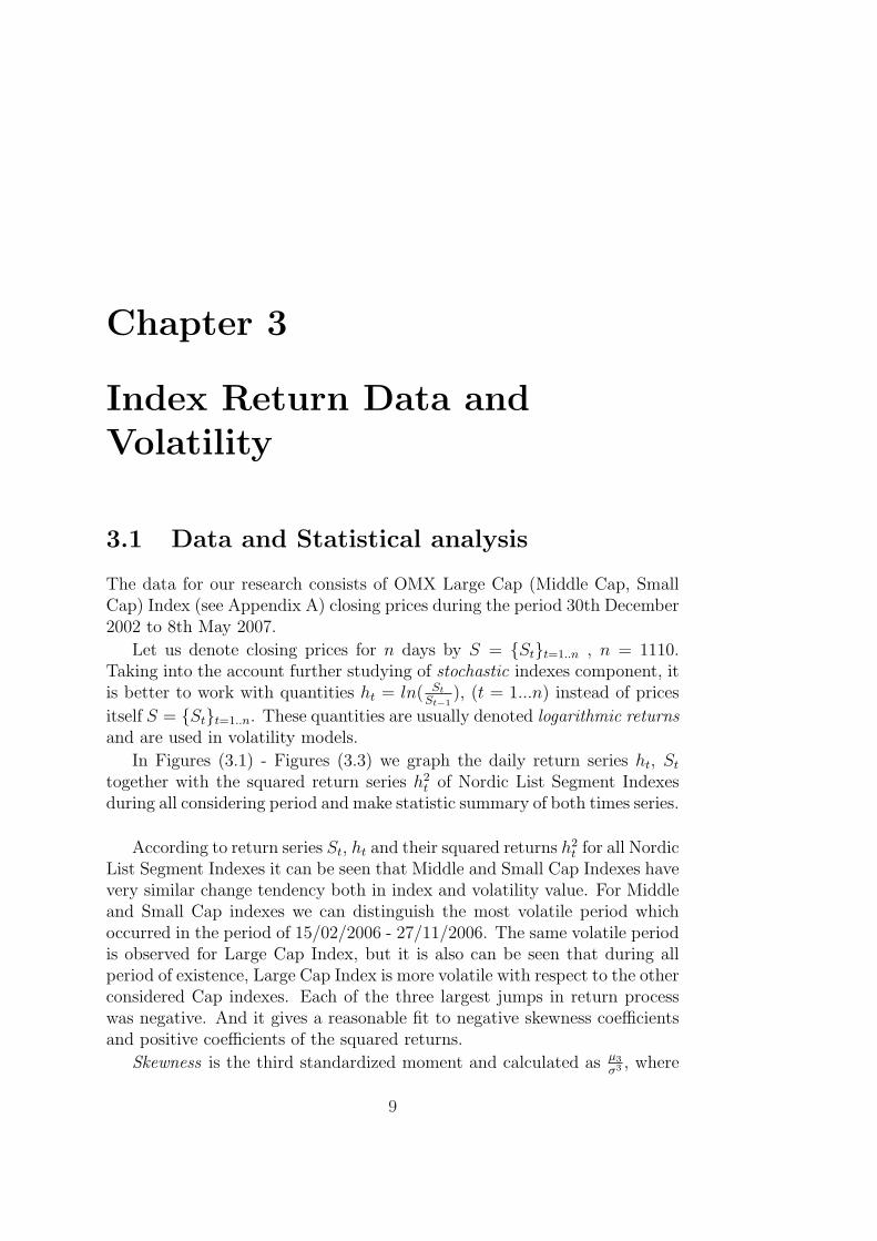
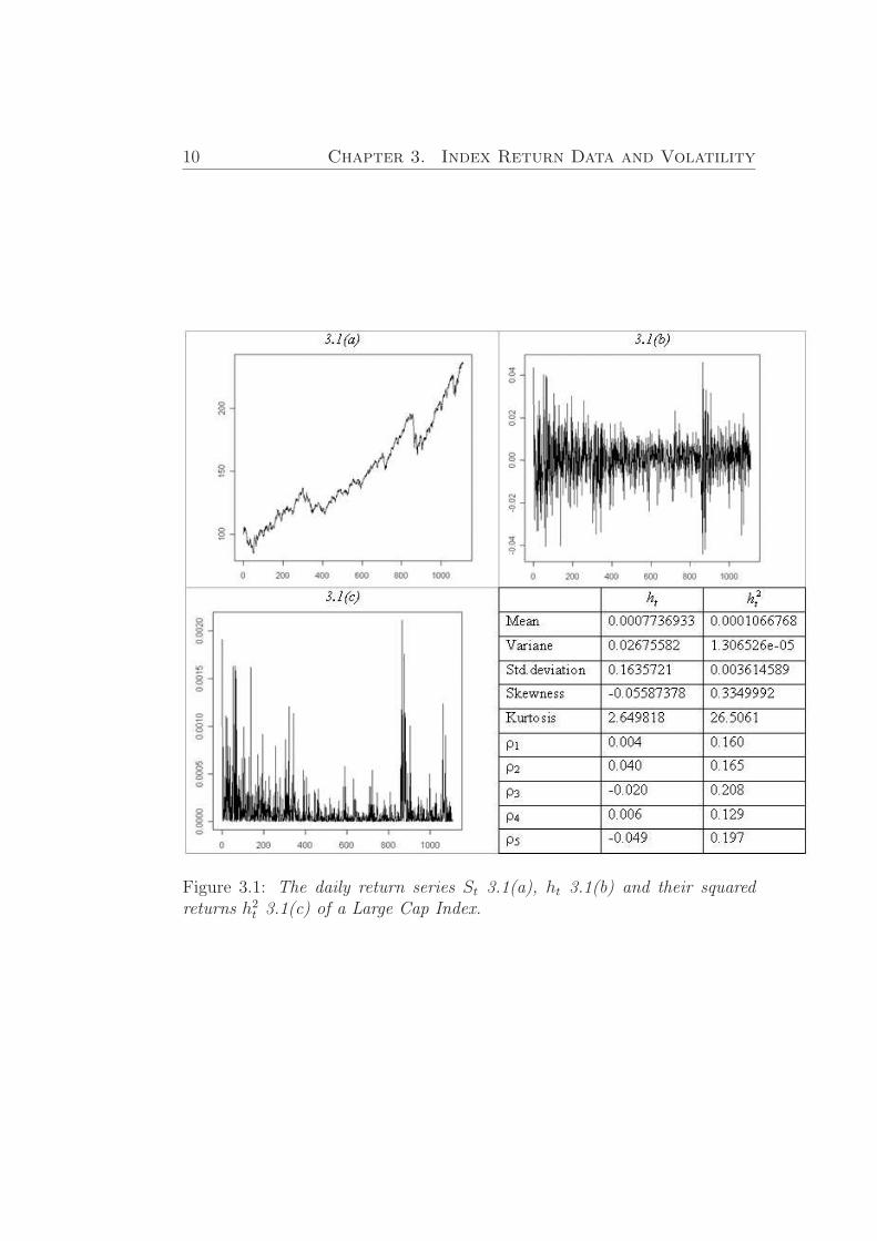
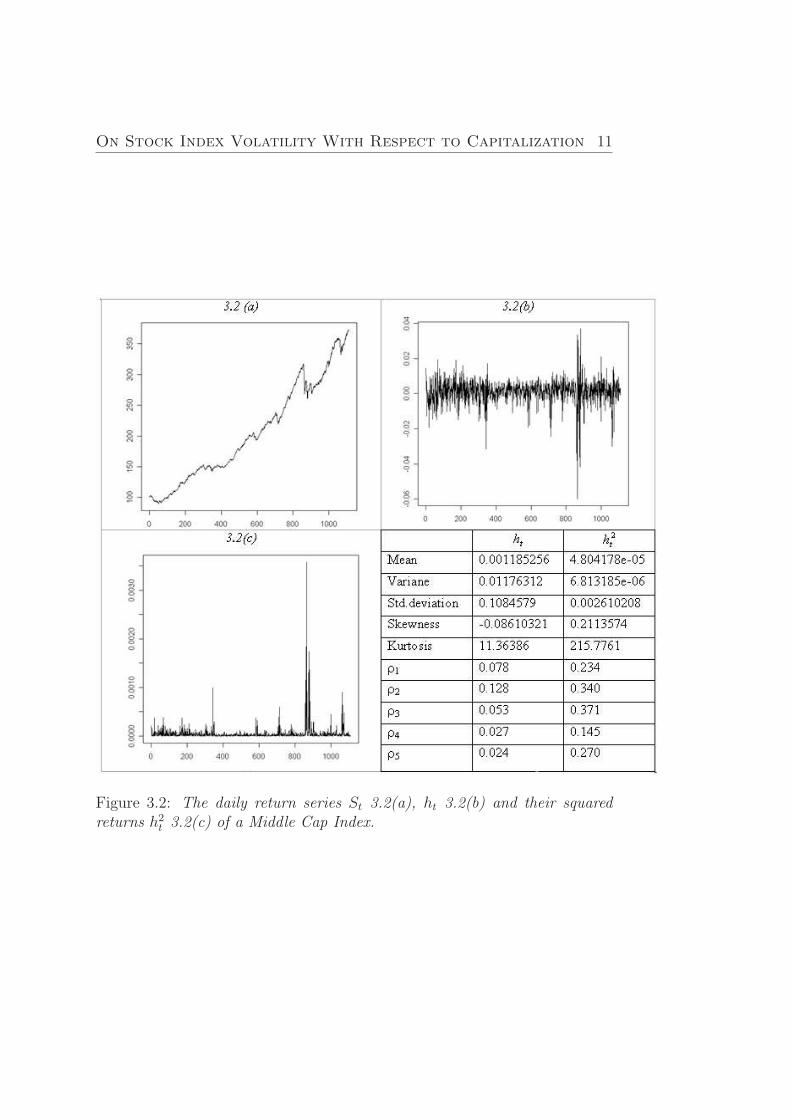
In Figures (3.1) - Figures (3.3) we graph the daily return series ht, St
together with the squared return series h2t of Nordic List Segment Indexes
during all considering period and make statistic summary of both times series.
According to return series St, ht and their squared returns h2t for all Nordic
List Segment Indexes it can be seen that Middle and Small Cap Indexes havevery similar change tendency both in index and volatility value. For Middleand Small Cap indexes we can distinguish the most volatile period whichoccurred in the period of 15/02/2006 - 27/11/2006. The same volatile periodis observed for Large Cap Index, but it is also can be seen that during allperiod of existence, Large Cap Index is more volatile with respect to the otherconsidered Cap indexes. Each of the three largest jumps in return processwas negative. And it gives a reasonable fit to negative skewness coefficientsand positive coefficients of the squared returns.
Skewness is the third standardized moment and calculated as µ3
σ3 , where
9
10 Chapter 3. Index Return Data and Volatility
Figure 3.1: The daily return series St 3.1(a), ht 3.1(b) and their squaredreturns h2
t 3.1(c) of a Large Cap Index.
On Stock Index Volatility With Respect to Capitalization 11
Figure 3.2: The daily return series St 3.2(a), ht 3.2(b) and their squaredreturns h2
t 3.2(c) of a Middle Cap Index.
12 Chapter 3. Index Return Data and Volatility
Figure 3.3: The daily return series St 3.3(a), ht 3.3(b) and their squaredreturns h2
t 3.3(c) of a Small Cap Index.
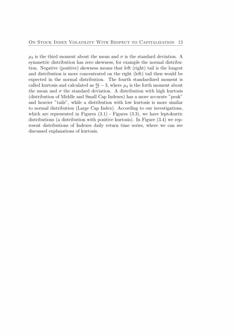
On Stock Index Volatility With Respect to Capitalization 13
µ3 is the third moment about the mean and σ is the standard deviation. Asymmetric distribution has zero skewness, for example the normal distribu-tion. Negative (positive) skewness means that left (right) tail is the longestand distribution is more concentrated on the right (left) tail then would beexpected in the normal distribution. The fourth standardized moment iscalled kurtosis and calculated as µ4
σ4 − 3, where µ4 is the forth moment aboutthe mean and σ the standard deviation. A distribution with high kurtosis(distribution of Middle and Small Cap Indexes) has a more accurate ”peak”and heavier ”tails”, while a distribution with low kurtosis is more similarto normal distribution (Large Cap Index). According to our investigations,which are represented in Figures (3.1) - Figures (3.3), we have leptokurticdistributions (a distribution with positive kurtosis). In Figure (3.4) we rep-resent distributions of Indexes daily return time series, where we can seediscussed explanations of kurtosis.
14 Chapter 3. Index Return Data and Volatility
Figure 3.4: Distributions of daily return series ht of a Large, Middle andSmall Cap Indexes.
Chapter 4
Theory
4.1 Statistics
A short explanation of the statistics that will be used is presented. We willuse following notations.
X - discrete valued stochastic variable,
k - the summation index,
PX(k) - the probability that X takes value k.
The first moment is the mean and is defined as
E(X) =∑
k
kpX(k) (4.1)
and then the second moment
E(X2) =∑
k
k2pX(k) (4.2)
The variance is
V ar(X) = E(X2)− (E(X))2 (4.3)
orV ar(X) = E(X − E(X))2 (4.4)
Skewness is the third standardized moment and defined as
E((X − µ)3)
(V ar(X))32
(4.5)
15
16 Chapter 4. Theory
For a normal distribution the skewness is zero.Kurtosis is the fourth standardized moment and defined as
E((X − µ)4)
(V ar(X))2(4.6)
For a normal distribution the kurtosis is 3. A distribution with a kurtosisgreater than 3 has more heavy tails and called leptokurtic.
Correlation. The correlation between two random variables X and Y isdefined by
Corr(X,Y ) =Cov(X,Y )√
V ar(X)V ar(Y )(4.7)
Autocorrelation. The i the autocorrelation is defined as
Corr(Xt, Xt−i) =Cov(Xt, Xt−i)√
V ar(Xt)V ar(Xt−i)(4.8)
Partial autocorrelation. The partial autocorrelation is defined as the lastcoefficient in a linear projection of X on the n most resent values. Let usdenote this value as α
(n)n , if the constant for the process is zero then:
Yt+1 = α(n)1 Yt + α
(n)2 Yt−1 + α(n)
n Yt−n+1 (4.9)
4.2 Hypothesis tests
A hypothesis test is a way to analyze data and to understand if a certaincriteria is fulfilled or not. This can be tested in different ways and this sectionpresents the hypothesis tests which will be used in this thesis.
All tests have a corresponding p-value. This p-value measures the fact”how much we are against the null hypothesis”. In other words p-value isthe probability to obtain result as close to a given sample as possible. Thesmaller p-value, the more clearness we have against the null hypothesis.
Jarque-Bera test. The Jarque-Bera test is used to check whether a givensample of data is normal distributed or not. The sample Jarque-Bera statisticis calculated as:
(T − k)
6(S2 +
(K − 3)2
4), (4.10)
where
On Stock Index Volatility With Respect to Capitalization 17
T - number of observations,
k - number of estimated parameters,
S - skewness,
K - kurtosis.
It can be seen from the formula that the larger the Jarque-Bera statisticthe lower the probability of being sampled data normal distributed. It shouldbe noted that the Jarque-Bera test is χ2 - distributed with 2 degrees offreedom.
Ljung-Box test. The Ljung-Box test is used to check whether a givensample of data has significant autocorrelation or not. The Ljung-Box statisticis calculated as:
T (T + 2)k∑
i=0
r2i
T − i, (4.11)
where
T - number of observations,
k - number of lags,
ri - the ith autocorrelation.
If the Ljung-Box statistic is large then the probability that the processhas uncorrelated data decreases. It should be noted that the Ljung-Box testis χ2 - distributed with k degrees of freedom.
4.3 ARCH - Autoregressive conditional het-
eroskedasticity
To accommodate a problem of random surges of assets returns under calcu-lation of volatility we can use well-developed ARCH/GARCH models. TheARCH-model was presented by Engle (1982), [2]. The ARCH - model con-siders the volatility as a sum of constant basic volatility and linear functionof absolute values of several last price changes. At the same time the levelof volatility is calculated with following recursive formula (ARCH(q)):
18 Chapter 4. Theory
σ2t = α0 +
q∑i=1
αiht−i (4.12)
ht = σtεt, where εt ∼ N(0, 1) iid.
α0 > 0, α1 ≥ 0, i = 1...q
In the sense of prices these parameters can be interpreted as
α0 - constant basic volatility;
hi - previous change in price;
q - order of a model - amount of last price changes influence on activevolatility;
αi - weight coefficients defining the influence power of last price changes onactive volatility value.
4.4 Generalized ARCH - GARCH
The enlargement of ARCH model is generalized autoregressive conditionalheteroscedasticity, GARCH (Bollerslev, 1986, [1]), model for volatility, wherecurrent volatility is influenced by both the previous price change and pre-vious volatility estimation, [1]. According GARCH (p,q) model volatility iscalculated with following recursive formula:
σ2t = α0 +
q∑i=0
αih2t−i +
p∑j=1
βjσ2t−j (4.13)
ht = σtεt, where εt ∼ N(0, 1) iid.
α0 > 0, α1 ≥ 0, βj ≥ 0, i = 1...q, j = 1...p
p is - the order of the GARCH terms, - amount of previous volatility esti-mations which influence on active volatility;
βj - weight coefficients defining the influence power of last volatility estima-tions on active volatility value;
q - is the order of the ARCH terms.
On Stock Index Volatility With Respect to Capitalization 19
Theorem. The GARCH(p,q) process as defined in (4.13) is wide-sense sta-tionary with E(εt) = 0, var(εt) = α0(1− A(1)− B(1))−1 and cov(εi, εs) = 0for t 6= s if and only if (A(1) + B(1) < 1) where A(1) =
∑qi=1 αi and
B(1) =∑p
j=1 βj.Proof. See Bollerslev (1986) page 323.In most cases the amount of parameters in GARCH model is small, for
instance GARCH(1,1). We will focus on this model.

20 Chapter 4. Theory
Chapter 5
GARCH Model andEstimations
The GARCH model was introduced in Chapter 4. In this Chapter we considerGARCH(1, 1) model and its application to volatility investigations.
5.1 Daily GARCH (1, 1)-model
GARCH (1, 1) model:
σ2t = α0 + α1h
2t−1 + β1σ
2t−1, (5.1)
ht = σtεt (5.2)
εt ∼ N(0, 1), t = 1...N , N = 1110 (amount of considering trading days).α0 > 0, α1 ≥ 0, β1 ≥ 0 and α1 + β1 < 1.
5.2 Estimation
The most widely used and well-implemented in many software packagesmethod is maximum likelihood method. This method was introduced byBollerslev, Chou and Kroner (1992), Bera and Higgens (1993) and Boller-slev, Engle and Nelson (1994).
In current subsection we examine GARCH(1, 1) model on the Nordic ListSegment Indexes and conclude which model fits better.
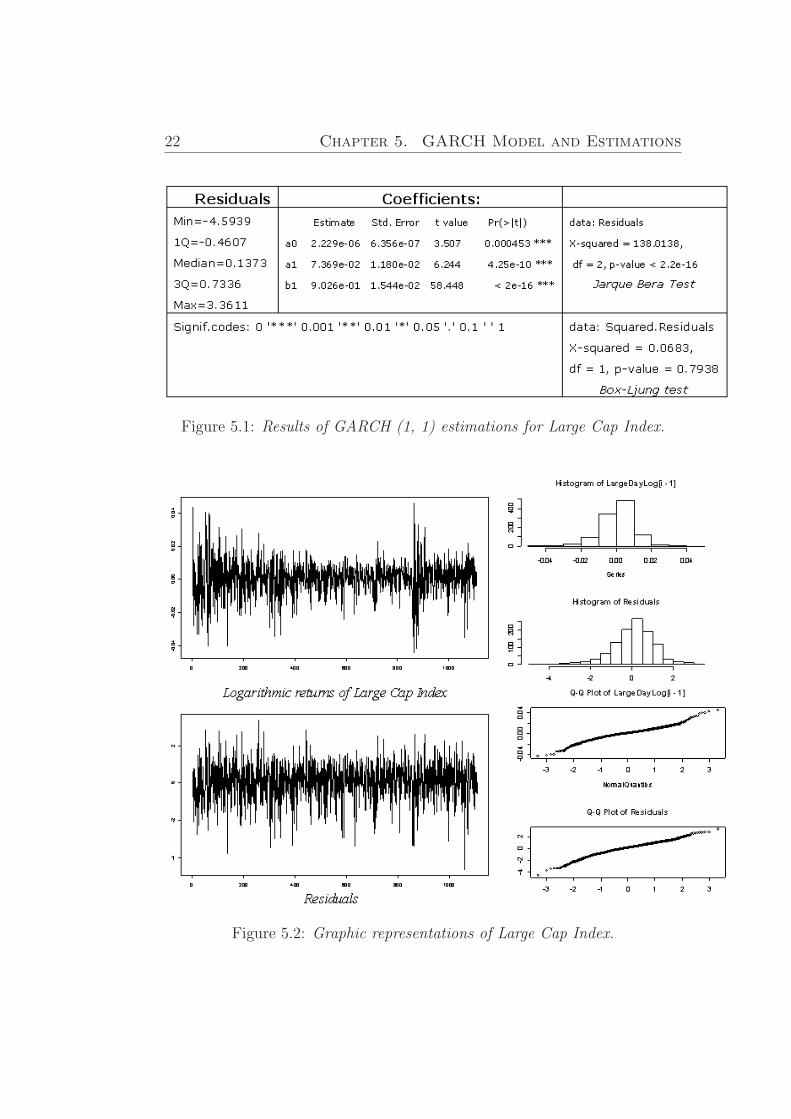
In Figure (5.1) and Figure (5.2) we represent the results from estimationsof a GARCH (1, 1) model for processes of Large Cap Index.
21
22 Chapter 5. GARCH Model and Estimations
Figure 5.1: Results of GARCH (1, 1) estimations for Large Cap Index.
Figure 5.2: Graphic representations of Large Cap Index.
On Stock Index Volatility With Respect to Capitalization 23
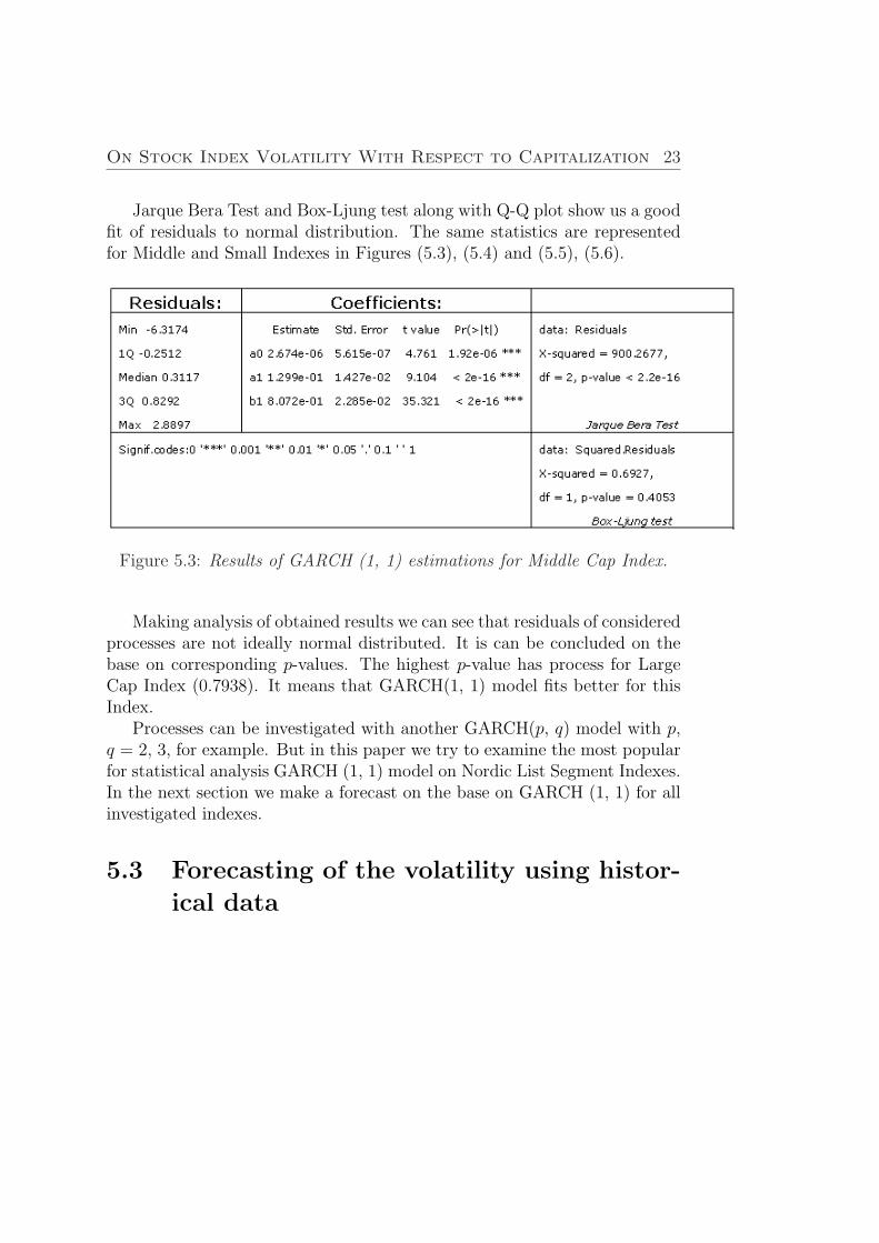
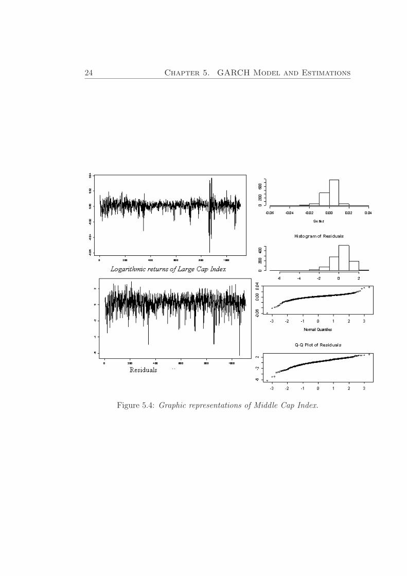
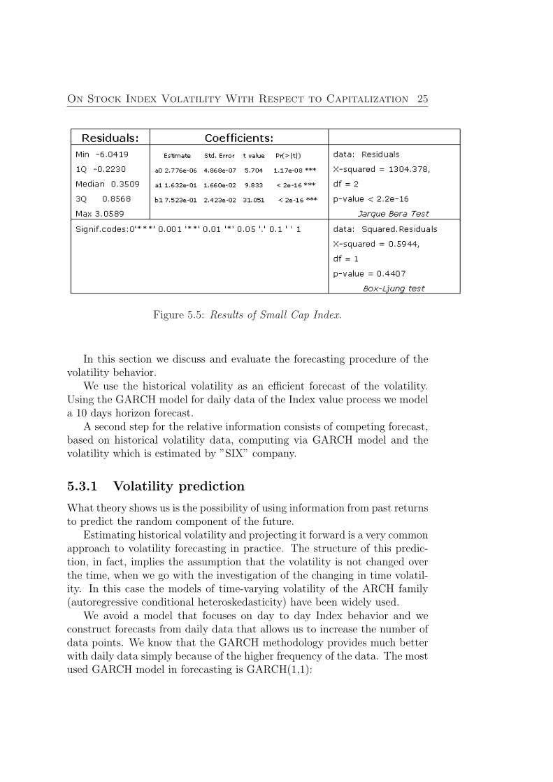
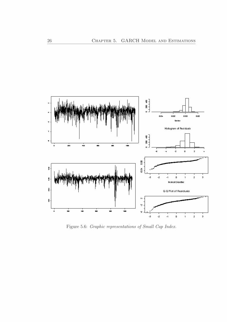
Jarque Bera Test and Box-Ljung test along with Q-Q plot show us a goodfit of residuals to normal distribution. The same statistics are representedfor Middle and Small Indexes in Figures (5.3), (5.4) and (5.5), (5.6).
Figure 5.3: Results of GARCH (1, 1) estimations for Middle Cap Index.
Making analysis of obtained results we can see that residuals of consideredprocesses are not ideally normal distributed. It is can be concluded on thebase on corresponding p-values. The highest p-value has process for LargeCap Index (0.7938). It means that GARCH(1, 1) model fits better for thisIndex.
Processes can be investigated with another GARCH(p, q) model with p,q = 2, 3, for example. But in this paper we try to examine the most popularfor statistical analysis GARCH (1, 1) model on Nordic List Segment Indexes.In the next section we make a forecast on the base on GARCH (1, 1) for allinvestigated indexes.
5.3 Forecasting of the volatility using histor-
ical data
24 Chapter 5. GARCH Model and Estimations
Figure 5.4: Graphic representations of Middle Cap Index.
On Stock Index Volatility With Respect to Capitalization 25
Figure 5.5: Results of Small Cap Index.
In this section we discuss and evaluate the forecasting procedure of thevolatility behavior.
We use the historical volatility as an efficient forecast of the volatility.Using the GARCH model for daily data of the Index value process we modela 10 days horizon forecast.
A second step for the relative information consists of competing forecast,based on historical volatility data, computing via GARCH model and thevolatility which is estimated by ”SIX” company.
5.3.1 Volatility prediction
What theory shows us is the possibility of using information from past returnsto predict the random component of the future.
Estimating historical volatility and projecting it forward is a very commonapproach to volatility forecasting in practice. The structure of this predic-tion, in fact, implies the assumption that the volatility is not changed overthe time, when we go with the investigation of the changing in time volatil-ity. In this case the models of time-varying volatility of the ARCH family(autoregressive conditional heteroskedasticity) have been widely used.
We avoid a model that focuses on day to day Index behavior and weconstruct forecasts from daily data that allows us to increase the number ofdata points. We know that the GARCH methodology provides much betterwith daily data simply because of the higher frequency of the data. The mostused GARCH model in forecasting is GARCH(1,1):
26 Chapter 5. GARCH Model and Estimations
Figure 5.6: Graphic representations of Small Cap Index.
On Stock Index Volatility With Respect to Capitalization 27
σ2t = α0 + α1h
2t−1 + β1σ
2t−1 (5.3)
β -weight coefficients defining the influence power of last volatility estima-tions on active volatility value;
α0- constant basic volatility;
hi = log Si
Si−1;
Si - value at the time i;
αi- weight coefficients defining the influence power of last price changes onactive volatility value, [4].
The GARCH(1,1) keeps the forecasting strategy when the variance ex-pected at a given date is a combination of a long run variance and the varianceexpected for last period, adjusted to take into account the size of last period’sobserved shock,[5].
5.3.2 Forecasting of 10-days - ahead volatility
By Using a GARCH(1,1) model, with the parameters α0 , α1 , β1 , whichwere carefully estimated from the past data, it is very reasonable to make aforecast for short horizon that will give us more precisely information of thefuture behavior of the volatility.
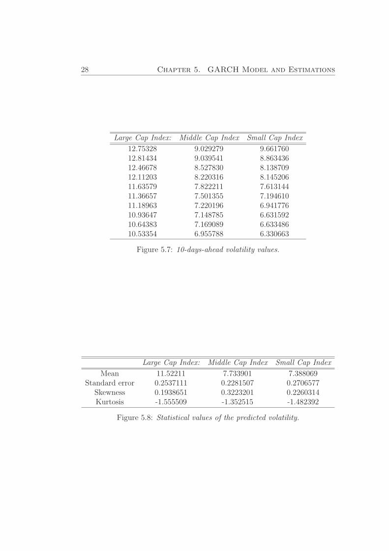
An investigation of the historical volatility considers the selection of asampling interval and the number of past values to include in the calculationand to apply equations. In the simulation we investigate the prediction ofthe volatility of a Large, Middle and Small Cap Indexes. The number of thepast observations is equal 22 days, forecast horizon is 10 days.
For the simulation we use R software.Data used for prediction 09.04.2007 - 08.05.2007.As the result we get 3 arrays with predicted values:We can see from the Table (5.7) that the forecasting volatility of Small
Cap Index is the lowest and the volatility of the Large Index is the highest.The standard error of the sample average of the mean is the ratio of the
volatility of the process in percent and square root of the number of historicaldaily price data, [5].
In the Table (5.8). introduced the investigation of the statistical valuesof forecasting volatility.
28 Chapter 5. GARCH Model and Estimations
Large Cap Index: Middle Cap Index Small Cap Index
12.75328 9.029279 9.66176012.81434 9.039541 8.86343612.46678 8.527830 8.13870912.11203 8.220316 8.14520611.63579 7.822211 7.61314411.36657 7.501355 7.19461011.18963 7.220196 6.94177610.93647 7.148785 6.63159210.64383 7.169089 6.63348610.53354 6.955788 6.330663
Figure 5.7: 10-days-ahead volatility values.
Large Cap Index: Middle Cap Index Small Cap Index
Mean 11.52211 7.733901 7.388069Standard error 0.2537111 0.2281507 0.2706577
Skewness 0.1938651 0.3223201 0.2260314Kurtosis -1.555509 -1.352515 -1.482392
Figure 5.8: Statistical values of the predicted volatility.
On Stock Index Volatility With Respect to Capitalization 29
5.3.3 Results
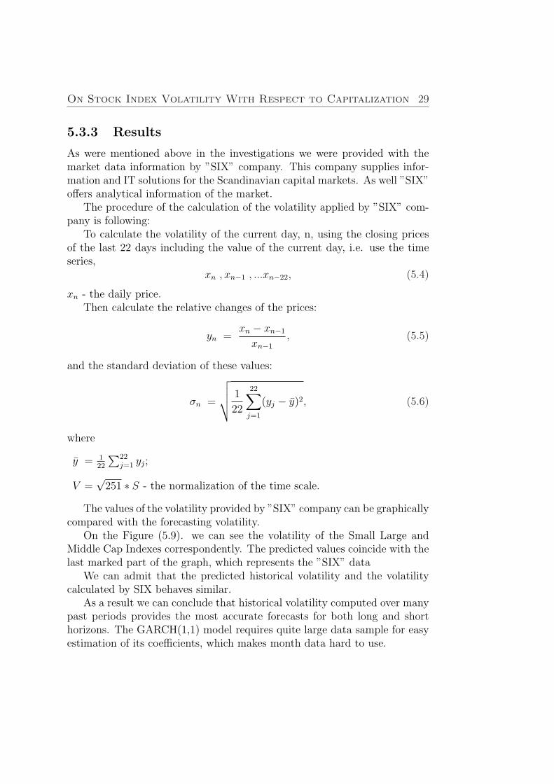
As were mentioned above in the investigations we were provided with themarket data information by ”SIX” company. This company supplies infor-mation and IT solutions for the Scandinavian capital markets. As well ”SIX”offers analytical information of the market.
The procedure of the calculation of the volatility applied by ”SIX” com-pany is following:
To calculate the volatility of the current day, n, using the closing pricesof the last 22 days including the value of the current day, i.e. use the timeseries,
xn , xn−1 , ...xn−22, (5.4)
xn - the daily price.Then calculate the relative changes of the prices:
yn =xn − xn−1
xn−1
, (5.5)
and the standard deviation of these values:
σn =
√√√√ 1
22
22∑j=1
(yj − y)2, (5.6)
where
y = 122
∑22j=1 yj;
V =√
251 ∗ S - the normalization of the time scale.
The values of the volatility provided by ”SIX” company can be graphicallycompared with the forecasting volatility.
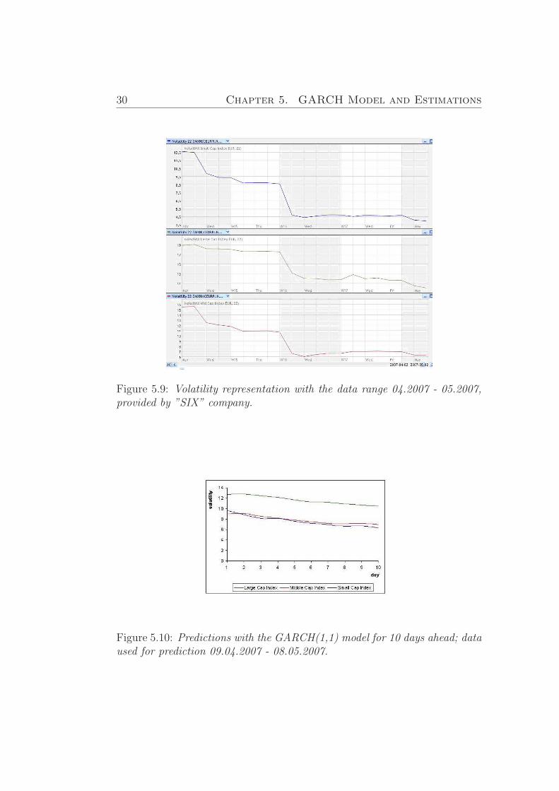
On the Figure (5.9). we can see the volatility of the Small Large andMiddle Cap Indexes correspondently. The predicted values coincide with thelast marked part of the graph, which represents the ”SIX” data
We can admit that the predicted historical volatility and the volatilitycalculated by SIX behaves similar.
As a result we can conclude that historical volatility computed over manypast periods provides the most accurate forecasts for both long and shorthorizons. The GARCH(1,1) model requires quite large data sample for easyestimation of its coefficients, which makes month data hard to use.
30 Chapter 5. GARCH Model and Estimations
Figure 5.9: Volatility representation with the data range 04.2007 - 05.2007,provided by ”SIX” company.
Figure 5.10: Predictions with the GARCH(1,1) model for 10 days ahead; dataused for prediction 09.04.2007 - 08.05.2007.
Chapter 6
Validation of the Heston Model
The Heston Model is a popular and widely used stochastic volatility models.It is tractable and stable in comparison with other Stochastic Volatility (SV)models.
In this section we introduce the simulation of the Heston model for ourinvestigation of the Indexes. We construct the process of the Heston modelvia Indirect Inference method by using the GARCH(1,1) as an auxiliarymodel.
6.1 The Heston Model
The Heston model is a mathematical model described the evolution of thevolatility of an underlying asset. It is a stochastic volatility model, i.e. itassumes that the volatility of the asset follows a random process. Let usdenote by νt the instantaneous volatility in the Heston model (1993), is aCox-Ingersoll-Ross (CIR) process, whose dynamic is given by:
dνt = κ(θ − νt)dt + σ√
νtdW νt (6.1)
where dW νt is (scalar) Brownian motion of the volatility process, which
in the Heston model is assumed to be correlated with the Brownian motiondW S
t , driving the asset returns, with the correlation parameter ρ.The basic Heston model assumes that St, the price of the asset, is deter-
mined by following stochastic process.
dSt = µStdt +√
νtStdW St (6.2)
where
µ - is the rate of return of the asset.
31
32 Chapter 6. Validation of the Heston Model
θ - is the long time volatility, or long run average price volatility; as t tendsto infinity, the expected value of νt tends to θ.
κ - is the rate at which νt reverts to θ, the mean reversion parameter.
σ - is the volatility of the volatility parameter, this determines the varianceof νt.
All the parameters µ, κ, θ, σ, ρ are time and state homogenous.
The Heston model has following parameters that need estimation: σ, κ, ρ,
µ, θ. It is known that the implied parameters and their time-series es-timate duplicate are different. We can not just use empirical estimates forthe parameters. Among the SV models, this problem is quite common. Andmost widespread solution is to find those parameters which produce the cor-rect prices, in our case of the Index. This is called an inverse problem , aswe solve for the parameters indirectly through some implied structure. Thisinverse problem can be solved by minimizing the variance between modelprices and market prices. We also need a constraint on the parameters toprevent the volatility reaching zero.
6.2 Estimation and testing model
We proceed as follows: we show that the Heston model can be nested intothe GARCH model by a suitable choice of the parameters. Via Indirectinference method as the auxiliary parameters we will use the parametersfrom GARCH simulations of the Index price process, to get the necessaryparameters of Heston model, than we will check if the obtained process willbe governed by GARCH model.
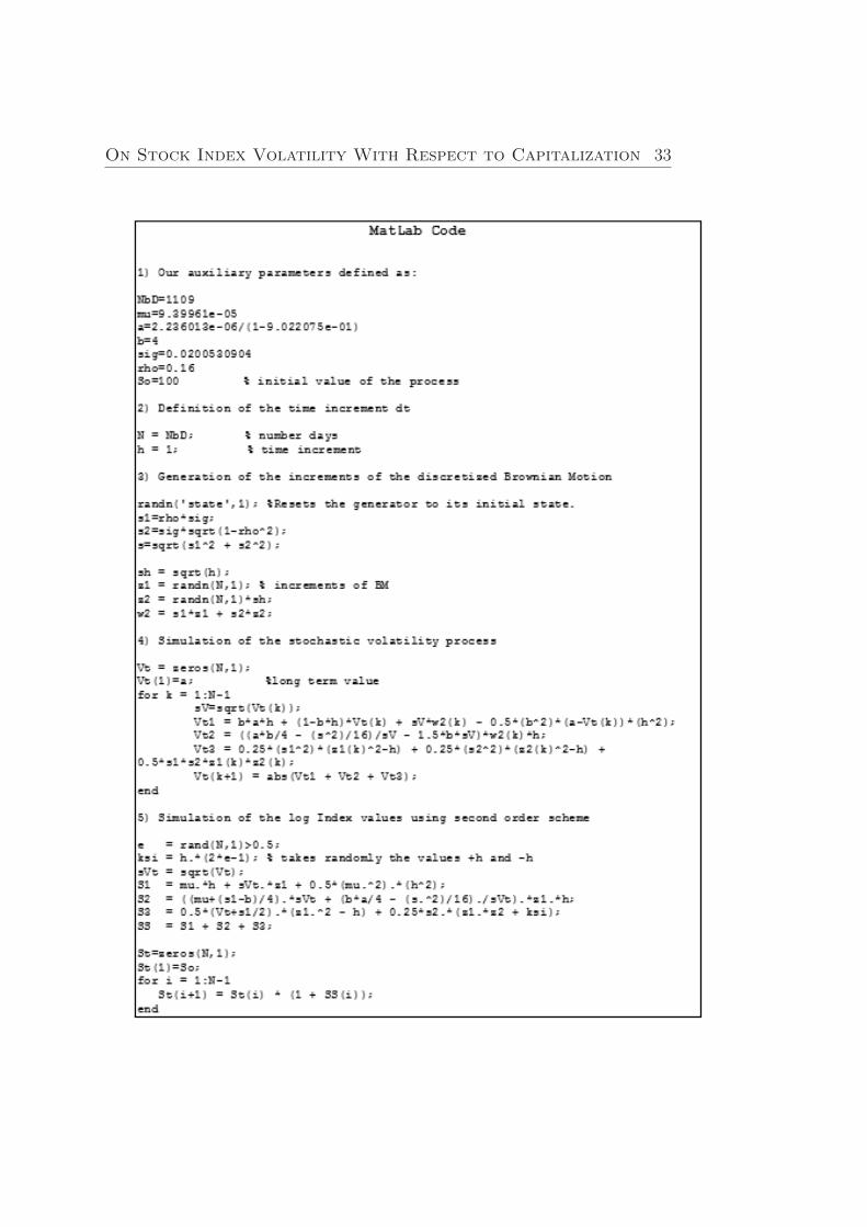
For the simulation of the Heston model we use Matlab software. It isa numerical computing environment and programming language, created byThe MathWorks. Matlab allows easy matrix manipulation, plotting of func-tions and data, implementation of algorithms, creation of user interfaces,and interfacing with programs in other languages. Although it specializes innumerical computing, an optional toolbox interfaces, allowing it to be partof a full computer algebra system.
Simulation of Heston model includes Monte Carlo method. This simula-tion was performed by discretising the stochastic processes using the imple-mentation of a second order scheme, [6].
On Stock Index Volatility With Respect to Capitalization 33
34 Chapter 6. Validation of the Heston Model
6.3 Simulated results
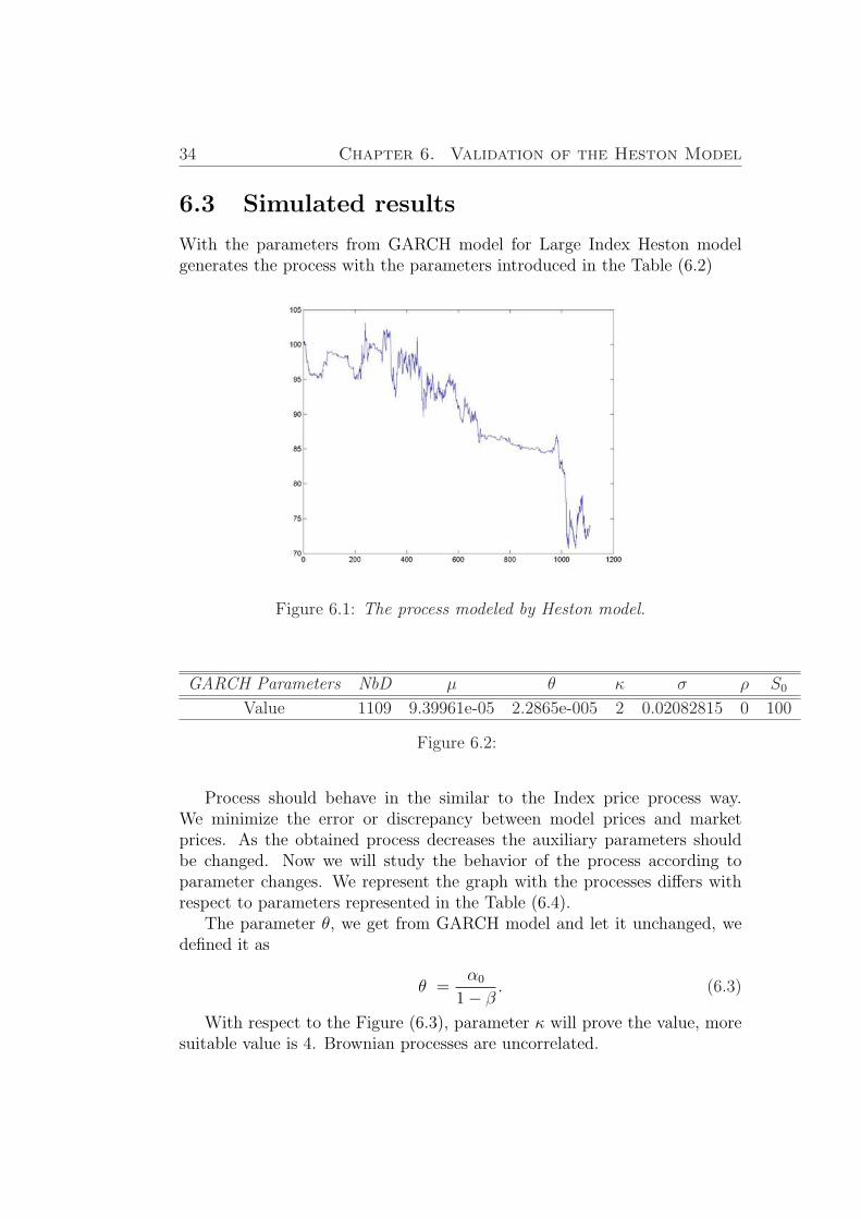
With the parameters from GARCH model for Large Index Heston modelgenerates the process with the parameters introduced in the Table (6.2)
Figure 6.1: The process modeled by Heston model.
GARCH Parameters NbD µ θ κ σ ρ S0
Value 1109 9.39961e-05 2.2865e-005 2 0.02082815 0 100
Figure 6.2:
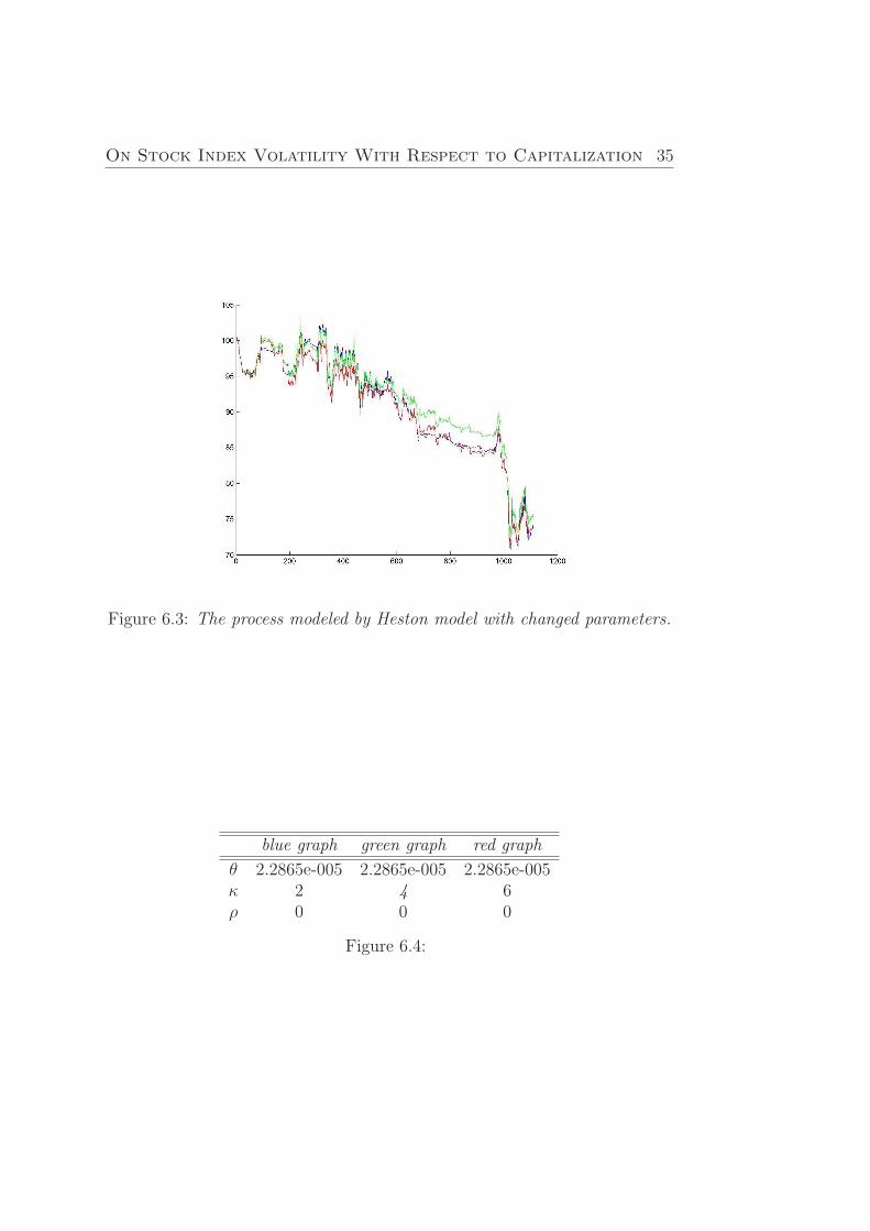
Process should behave in the similar to the Index price process way.We minimize the error or discrepancy between model prices and marketprices. As the obtained process decreases the auxiliary parameters shouldbe changed. Now we will study the behavior of the process according toparameter changes. We represent the graph with the processes differs withrespect to parameters represented in the Table (6.4).
The parameter θ, we get from GARCH model and let it unchanged, wedefined it as
θ =α0
1− β. (6.3)
With respect to the Figure (6.3), parameter κ will prove the value, moresuitable value is 4. Brownian processes are uncorrelated.
On Stock Index Volatility With Respect to Capitalization 35
Figure 6.3: The process modeled by Heston model with changed parameters.
blue graph green graph red graph
θ 2.2865e-005 2.2865e-005 2.2865e-005κ 2 4 6ρ 0 0 0
Figure 6.4:
36 Chapter 6. Validation of the Heston Model
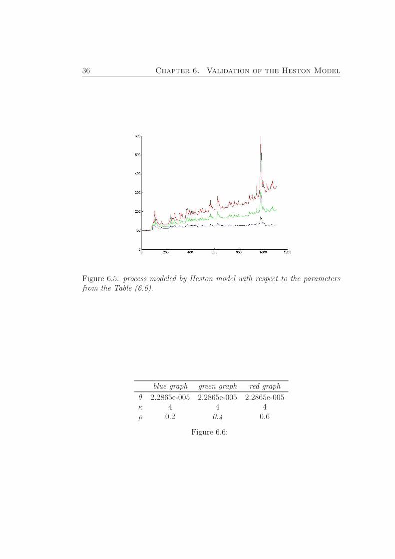
Figure 6.5: process modeled by Heston model with respect to the parametersfrom the Table (6.6).
blue graph green graph red graph
θ 2.2865e-005 2.2865e-005 2.2865e-005κ 4 4 4ρ 0.2 0.4 0.6
Figure 6.6:
On Stock Index Volatility With Respect to Capitalization 37
Figure (6.5) shows that the process behaves better when the parameterρ increases. ρ, the correlation between the log-returns and volatility of theIndex, affects the heaviness of the tails. If ρ > 0, then volatility will increaseas the Index value increases. And if ρ < 0, then volatility will increase whenthe Index value decreases. Let us take correlation equal 0.4.
6.4 GARCH simulations of the ”Heston pro-
cess”
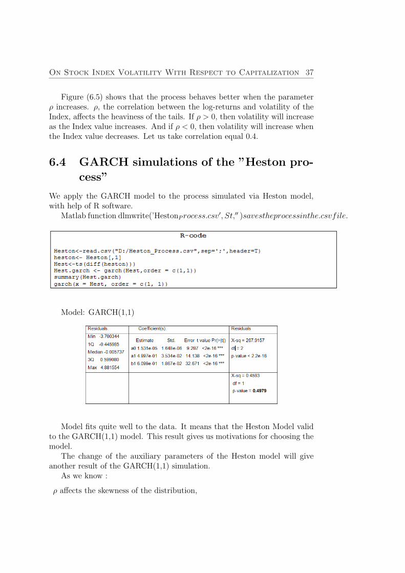
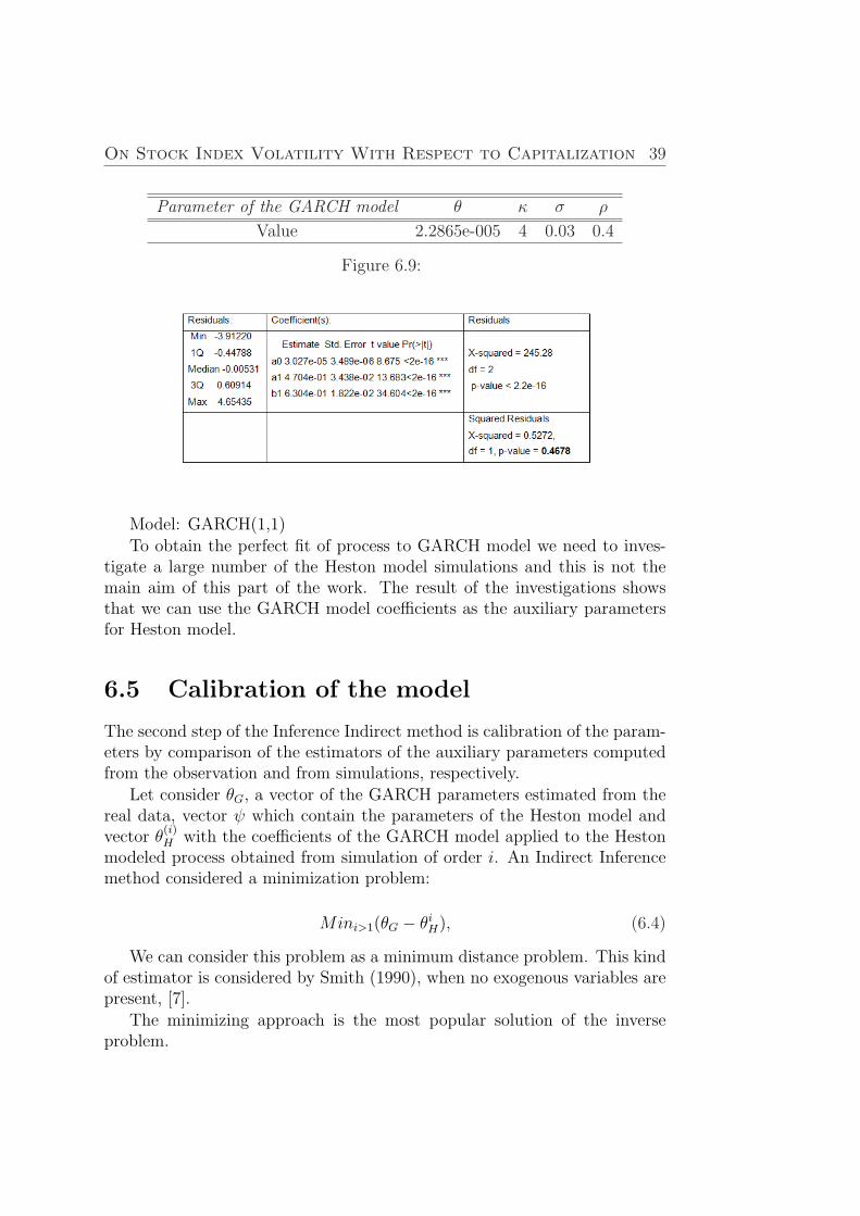
We apply the GARCH model to the process simulated via Heston model,with help of R software.
Matlab function dlmwrite(’HestonP rocess.csv′, St,′′ )savestheprocessinthe.csvfile.
Model: GARCH(1,1)
Model fits quite well to the data. It means that the Heston Model validto the GARCH(1,1) model. This result gives us motivations for choosing themodel.
The change of the auxiliary parameters of the Heston model will giveanother result of the GARCH(1,1) simulation.
As we know :
ρ affects the skewness of the distribution,
38 Chapter 6. Validation of the Heston Model
σ affects the kurtosis of the distribution.
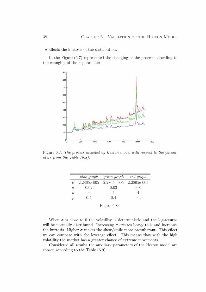
In the Figure (6.7) represented the changing of the process according tothe changing of the σ parameter.
Figure 6.7: The process modeled by Heston model with respect to the param-eters from the Table (6.8).
blue graph green graph red graph
θ 2.2865e-005 2.2865e-005 2.2865e-005σ 0.02 0.03 0.04κ 4 4 4ρ 0.4 0.4 0.4
Figure 6.8:
When σ is close to 0 the volatility is deterministic and the log-returnswill be normally distributed. Increasing σ creates heavy tails and increasesthe kurtosis. Higher σ makes the skew/smile more protuberant. This effectwe can compare with the leverage effect. This means that with the highvolatility the market has a greater chance of extreme movements.
Considered all results the auxiliary parameters of the Heston model arechosen according to the Table (6.9).
On Stock Index Volatility With Respect to Capitalization 39
Parameter of the GARCH model θ κ σ ρ
Value 2.2865e-005 4 0.03 0.4
Figure 6.9:
Model: GARCH(1,1)
To obtain the perfect fit of process to GARCH model we need to inves-tigate a large number of the Heston model simulations and this is not themain aim of this part of the work. The result of the investigations showsthat we can use the GARCH model coefficients as the auxiliary parametersfor Heston model.
6.5 Calibration of the model
The second step of the Inference Indirect method is calibration of the param-eters by comparison of the estimators of the auxiliary parameters computedfrom the observation and from simulations, respectively.
Let consider θG, a vector of the GARCH parameters estimated from thereal data, vector ψ which contain the parameters of the Heston model andvector θ
(i)H with the coefficients of the GARCH model applied to the Heston
modeled process obtained from simulation of order i. An Indirect Inferencemethod considered a minimization problem:
Mini>1(θG − θiH), (6.4)
We can consider this problem as a minimum distance problem. This kindof estimator is considered by Smith (1990), when no exogenous variables arepresent, [7].
The minimizing approach is the most popular solution of the inverseproblem.
40 Chapter 6. Validation of the Heston Model
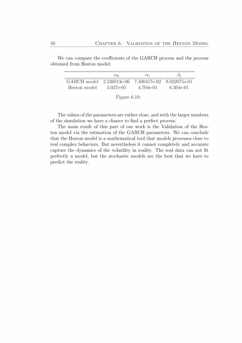
We can compare the coefficients of the GARCH process and the processobtained from Heston model:
α0 α1 β1
GARCH model 2.236013e-06 7.400417e-02 9.022075e-01Heston model 3.027e-05 4.704e-01 6.304e-01
Figure 6.10:
The values of the parameters are rather close, and with the larger numbersof the simulation we have a chance to find a perfect process.
The main result of this part of our work is the Validation of the Hes-ton model via the estimation of the GARCH parameters. We can concludethat the Heston model is a mathematical tool that models processes close toreal complex behaviors. But nevertheless it cannot completely and accuratecapture the dynamics of the volatility in reality. The real data can not fitperfectly a model, but the stochastic models are the best that we have topredict the reality.
Chapter 7
Conclusions
There were two objectives in this thesis. The first objective was to investigatevolatility of OMX indexes with respect to their capitalization and the secondwas to estimate Heston model. This analysis allows us to better understandthe drivers behind volatility of financial asset.
The methodology used in this research uses special literature to solvesome of statistical problems. The literature helped us with choosing modelsfor our investigations and make correct conclusions.
The GARCH(1,1) model was chosen for analysis of financial data. Ac-cording to made investigations we can conclude that for three chosen indexes(Small Cap Index, Mid Cap Index and Large Cap Index) Large Cap Index ismore volatile. It is an unusual result. The common assumption is that themore cap index we have the less it is volatile. One way to explain the resultwe obtained is that some companies in OMX Large Cap Index have a veryhigh volatility.
41

42
Bibliography
[1] T. Bollerslev. (1986)Generalised Autoregressive Conditional Heteroscedasticity. Journal ofEconometrics, 31, 307 – 327.
[2] R. Engle (1982)Autoregressive Conditional Heteroscedasticity with Estimates of theVariance of UK Inflation. Econometrica, 50, 987 – 1008.
[3] RiskMetrics Group (December 1996)RiskMetrics Technical Document. RiskMetrics Group.
[4] N. Shiryaev (1999)Essentials of Stochastic Finance: Facts; Models; Theory. by World Sci-entific Publishing Co. Pte. Ltd.
[5] Figlewski (2004)Forecasting Volatility. Final Draft.
[6] Glasserman (2003)Monte Carlo Methods in Financial Engineering.XIV, 602 p.
[7] C. Gourieroux, A. Monfort,. Renault. (Dec. 1993)Indirect inference. Journal of applied econometrics.
[8] Nimalin Moodley (2005)The Heston Model:A Practical Approach. Faculty of Science, Universityof the Witwatersrand,Johannesburg,South Africa.
[9] Chiara Monfardini (June 1997)Estimating stochastic volatility models through indirect inference. Euro-pean University Institute.
[10] Torben G. Andersen, Tim Bollerslev. (June 16, 2005)Volatility and Correlation Forecasting.
43

[11] Richard Hawkes, Paresh Date (June 16, 2006)Surveillance of the interaction parameter of the Ising model.
[12] Jean-Pierre Fouque, George Papanicolaou (1995)Derivatives in Financial Markets with Stochastic Volatility. Cambridgeuniversity press
44
Appendix
OMX Nordic Exchange The following information about OMX NordicExchange is taken from http://www.omxgroup.com
”OMX Nordic Exchange serves as a central gateway to the Nordic andBaltic financial markets, promoting greater interest, opportunity and invest-ment in the whole region. Today, the Nordic Exchange offers ease of accessto more than 80 percent of the exchange trading in the Nordic and Balticcountries. To fully utilize the potential of the two markets there are twolists: The Nordic list and The Baltic list. The Nordic list comprises thecompanies listed on the exchanges in Copenhagen, Stockholm, Helsinki andIceland. The Baltic list includes the companies listed on the exchanges inTallinn, Riga and Vilnius.
OMX Index Types
Gross Index (GI): To reflect the true performance of an index, dividendsare reinvested in the gross index. The reinvestment is carried out byadjusting the pi,t-1 in the denominator in the index with subtractionof dividends from this price on the ex-dividend date t. This adjustmentreinvests the dividend in all index constituents in proportion to theirrespective weights.
Net Index (NI): Same as the gross index, but the dividend is reinvestedafter deduction of withholding tax.
Price Index (PI): In a price index, no cash dividend is reinvested in theindex. Hence, the price index only yields the performance of stockprice movements. The difference in rate of return for the total andprice return version of an index is attributable to the dividend yield ofthe index.
45
Capped Index (Cap): In a capped index, the weight of the index constituentshave an upper limit. If an index constituent exceeds the upper limit,its weight in index is adjusted to the upper limit.
Nordic List Segment Indexes. PI, GI The Nordic list segmentindexes comprising Nordic Large Cap, Mid Cap and Small Cap are based onthe three market capitalization groups. The aim of the division into marketcapitalization groups is to capture the current status and changes in themarket with company size taken into account. The base date for the OMXNordic list index is December 30, 2002, with a base value of 100. The indexis available as PI and GI.”
46