MODELING VOLATILITY IN INTERNATIONAL STOCK MARKETS

MODELING VOLATILITY IN INTERNATIONAL STOCK MARKETS

JOSE DIAS CURTO

ISCTE Business School (IBS),

Department of Quantitative Methods

Complexo INDEG/ISCTE, Av. Prof. Anıbal Bettencourt

1600-189 Lisboa, Portugal

Phone: 351 21 7826100. Fax: 351 217958605.

E-mail: [email protected].

FRANCISCO RIBEIRO DE MATOS

ISCTE Business School (IBS).

Abstract

Since the introduction of VEC model (Bollerslev, Engle and Wooldrigde, 1988) several

multivariate GARCH models have been proposed to estimate conditional covariance matrices.

As most of the empirical applications assume normal innovations, in this paper we propose

the BEKK(1,1,1) model’s estimation for five stock markets indices, considering a multivariate

student’s t distribution. Furthermore, in order to capture the asymmetric effect on volatility,

we introduce a new leverage effect in the multivariate model without losing the Student’s t

innovations hypothesis. Based on estimated models we draw conclusions about the volatility

interactions across international stock markets located in different economic regions such as

Europe, United States and Asia.

Keywords: Multivariate GARCH Models, Volatility dynamics, Student’s t distribution,

Leverage effects.

JEL classification: C13, C32, C51, G15

1

1 Introduction

Modeling volatility becomes an important financial issue. From the correct configuration of

hedging strategies to the estimation of portfolio VaR, the volatility plays an important role.

Moreover, the interaction between international stocks markets has been growing in such a way

that the correct hedging position for an international portfolio depends from the accuracy to

correctly estimate the relationships across markets volatility.

The Autoregressive Conditional Heteroscedasticity Model (Engle, 1982) and all its variants

provide an important univariate framework to model the volatility in capital markets. Since

the appearance of the ARCH model, several developments have been made to improve the

characteristics of this new framework and to model the stylized facts of financial returns such as

the persistence and asymmetric effects on volatility. Important extensions of the ARCH model

include the GARCH model (Bollerslev, 1986) and the EGARCH model (Nelson, 1991). In the

original form these models assume a Gaussian distribution for innovations. However, in order

to capture the excess of kurtosis stylized fact of returns, other distributions have been adopted

namely the Student’s t (Bollerslev, 1987).

Despite the vast univariate GARCH models literature, it is commonly accepted that in-

ternational stock markets are becoming more integrated and volatility depends not exclusively

from domestic factors. In fact, the behavior of prices in relevant stock markets influences the

other markets in the world and the integration of international markets tends to increase with

geographic proximity. Thus, the Multivariate Generalization of the ARCH theory becomes

inevitable.

Bollerslev, Engle and Wooldrigde (1988) proposed the first multivariate GARCH model, the

VEC model, that allows simultaneous estimation of conditional variances and covariances. De-

spite its generalization, a large number of parameters has to be estimated and several restrictions

are needed to assure the positivity of the conditional covariance matrix. Thus, it is somewhat

unpractical working with more than 3 or 4 series.

Models developed after VEC intend to be a commitment between parsimony and flexibility.

The BEKK model (Engle and Kroner, 1995) is less general than VEC but it is parameterized

in such a way that it is possible to guarantee the positivity of the conditional covariance matrix

with some weak conditions.

The Factor ARCH model (Engle, Ng and Rothschild, 1990) reduces the number of parameters

considering that co-movements of data are driven by a small number of common underlying

2

dimensions which are named by factors.

The conditional correlation models are based on a two steps estimation procedure. The condi-

tional variances are estimated under univariate GARCH models and the conditional covariances

are estimated after that. The two most important models in this class are the Bollerslev (1990)

Conditional Constant Correlation model where it is assumed that correlations are constant over

time and the Dynamics Conditional Correlations model, Engle (2002) and Tse and Tsui (2002),

where correlations change over time. For a recent survey on multivariate GARCH models see

Silvennoinen and Terasvirta (2006).

The main purpose of this paper is to analyze the volatility dynamics in the international

stock markets based on the extensive theory of Multivariate GARCH models. We selected

five stock indices (DAX30, FTSE100, S&P500, NIKKEI225 and DJIA30) which are the most

representative in their geographic regions (United States, Europe and Asia).

The conditional covariance matrix is parameterized as the BEKK (1,1,1) model that allows

most of the interaction between financial stock markets volatility to be captured with flexibility

and without parameters restrictions to assure the positivity of the conditional covariance matrix.

Furthermost, we intend to model the stylized facts of returns in order to fully understand the

international stock markets volatility dynamics. We assume that innovations follow a Student’s

t distribution with v degrees of freedom to capture the leptokurtic behavior of financial returns

and we compare the model’s goodness-of-fit with the BEKK normal distributed innovations

model by using the maximum log likelihood value and two information criteria.

In addition we propose the introduction of a simple leverage effect on volatility. With this

and under certain conditions, we expect to model the asymmetric behavior observed in the stock

returns volatility as noted by Black (1976). The leverage effect is modeled by a multivariate

generalization of the univariate GJR model; when this effect is introduced, the assumption of

Student’s t distributed innovations is maintained.

Once the models are estimated, the results are interpreted in order to analyze the dynamics

of volatility in the five international stock markets.

The paper is organized as follows. Next section presents a brief description of VEC and

BEKK models and discusses the properties of the model under estimation with the leverage

extension included. Data and methodology appear in the third section and the estimation

results are presented and discussed in section 4. The last section provides the conclusions and

final remarks.

3

2 Multivariate GARCH Models

2.1 VEC and BEKK models

The univariate GARCH models objective is to estimate the conditional variance of returns

denoted by σ2t or ht. In a Multivariate framework the purpose is to estimate the conditional

covariance matrix of at least two series of financial returns denoted by Ht.

The first multivariate formulation was introduced by Bollerslev, Engle and Wooldrigde (1988)

and was named by the VEC model. In this model the second conditional moments of a financial

return series depend from the lagged squared innovations, the cross product of the innovations

and the lagged values of past conditional variances and covariances.

The equation of the VEC(p, q) model is as follows:

ht = c +q∑

i=1

Aiηt−i +p∑

i=1

Giht−i, (1)

where ht = vech(Ht) and ηt−i = vech(utu′t), Ai and Gi represent squared matrices with para-

meters of order (N + 1)N/2 and c is a (N + 1)N/2 × 1 vector of parameters, where N is the

number of financial assets.

As an example, the trivariate VEC(1,1) is represented in the following matrix form:

Ht =

c1

c2

c3

c4

c5

c6

+

a11 a12 a13 a14 a15 a16

a21 a22 a23 a24 a25 a26

a31 a32 a33 a34 a35 a36

a41 a42 a43 a44 a45 a46

a51 a52 a53 a54 a55 a56

a61 a62 a63 a64 a65 a66

u21,t−1

u1,t−1u2,t−1

u1,t−1u3,t−1

u22,t−1

u2,t−1u3,t−1

u23,t−1

+

g11 g12 g13 g14 g15 g16

g21 g22 g23 g24 g25 g26

g31 g32 g33 g34 g35 g36

g41 g42 g43 g44 g45 g46

g51 g52 g53 g54 g55 g56

g61 g62 g63 g64 g65 g66

h11,t−1

h12,t−1

h13,t−1

h22,t−1

h23,t−1

h33,t−1

This is a general framework to model conditional variances since the VEC model includes

all the possible interactions between the financial series under analysis. In this model, besides

the dependence on its own lagged squared innovations and past conditional variances, like the

univariate GARCH models, the conditional variance also depends on the lagged squared inno-

vations from the other time series, on the cross products of the innovations, on the conditional

variances of other time series and on the conditional covariances.

Despite its ability to describe the interaction on volatility, some problems arise when the

VEC model is generalized. First, in a VEC(1,1) model with three financial assets (N = 3) the

number of parameters to estimate is 78. If we consider N = 4, the number of parameters to

estimate rises to 210. As the number of parameters increases, the VEC framework becomes

impractical for estimation. Second, to assure that the covariance matrix is positive definite, the

4

parameters included in the matrices must be greater than 0. This also becomes troublesome

because a series of parameters restrictions must be imposed to assure their positiveness.

As one of the VEC model major drawbacks is the difficulty to assure the positivity of Ht

without imposing strong parameters restrictions, Engle and Kroner (1995) proposed a new

formulation for Ht that imposes its positivity by construction. This new parametrization is

known as the BEKK1 model.

The BEKK(p,q,K) model is defined as:

Ht = C∗′C∗ +K∑

k=1

q∑

j=1

A∗′

jkut−ju′t−jA

∗jk +

K∑

k=1

p∑

i=1

G∗′ikHt−iG

∗ik, (2)

where C, A, and G are (N ×N) matrices of parameters, but C is upper triangular.

The K element refers to the generality of the model and a higher K implies a more general

process2. Nevertheless, most of the practical applications of the BEKK (1,1,K) model set K = 1,

which makes the process represented by:

Ht = C∗′C∗ + A∗′

11ut−1u′t−1A

∗11 + G∗′

11Ht−1G∗11. (3)

BEKK models the dynamics of conditional variances with fewer parameters than the VEC

model. However, the interpretation of the parameters is not as easy as in the VEC model. The

model represents a direct multivariate generalization of the univariate GARCH model. In fact,

if N = 1 and K = 1, the equation (2) reduces to the GARCH equation.

The number of parameters to estimate in a BEKK(1,1,1) model is given by the N(5N +1)/2.

However, there are still too many parameters when the number of series is greater than 3 or

4. For 5 time series, for example, the number of parameters to estimate in a BEKK (1,1,1) is

65 against 465 in a VEC(1,1). The reduction in the number of parameters is possible because

most parameters for the conditional covariances are obtained from parameters associated to the

conditional variances.

2.2 A New Multivariate GARCH Model

In this paper we propose a BEKK(1,1,1) model to estimate the conditional covariance matrix for

the five stock indices and to conclude about the volatility dynamics. Despite the reduced gen-1The name BEKK results from a work in multivariate models developed by Baba, Engle, Kraft and Kroner.2Engle and Kroner(1995) presented the conditions for K that allows the model to achieve the equivalent

generality of the VEC Model.

5

erality when compared to the VEC(1,1) model, it is able to clarify the dynamics on conditional

variances and covariances of the five stock markets returns.

The standard BEKK(1,1,1) model is defined as:

Rt = Ω + ut (4)

ut|Ψt−1 ≈ N(0,Ht) (Model 1) or ut|Ψt−1 ≈ t(0,Ht, v) (Model 2) (5)

Ht = C∗′C∗ + A∗′

11ut−1u′t−1A

∗11 + G∗′

11Ht−1G∗11 (6)

where Ω is a vector of constants.

The VEC (1,1) positive parameters restrictions are not needed as the second and third terms

of (6) are quadratic forms and C∗′C∗ is symmetric and positive definite; thus the positive defi-

niteness of Ht is guaranteed. This BEKK(1,1,1) model implies the estimation of 70 parameters

in model 1 and 71 parameters in model 2.

The BEKK(1,1,1) standard formulation accounts for the most important volatility dynamics

but does not allow the asymmetric effect on volatility that is common in most of stock market

returns.

However, the multivariate framework allows the volatility asymmetric effect to be analyzed

not only in terms of domestic markets but also in terms of the asymmetric response to negative

shocks in foreign index returns. To model the asymmetric response to shocks in returns volatility,

we propose the introduction of a leverage effect in the BEKK formulation, based on the univariate

GJR model3. The leverage effect is defined as:

L = lN∑

i=1

diu2i,t−1I (7)

where l represents the leverage coefficient, di are dummy variables that assume the value 1 if

ui,t−1 < 0 and 0 otherwise and I is a (N ×N) identity matrix.

With these added terms we assume that the leverage effect is the same for all stock markets

and investors react in the same way if there is a negative shock in one of the markets. This

assumption is supported on fact that stock markets are becoming more integrated and investors

tend to increase their international diversification despite the subject of home bias. Thus, we

assume that investors see global markets as a whole. It is also assumed that the leverage effect

only implies on conditional variances.3Note that Hafner and Herwartz (1998) have study the volatility impulse response for multivariate GARCH

models in order to estimate the dynamics in bivariate exchange rate series.

6

According to this new formulation, expression (6) becomes:

Ht = C∗′C∗ + A∗′

11ut−1u′t−1A

∗11 + G∗′

11Ht−1G∗11 + Lt−1. (8)

where the Lt−1 matrix is as follows:

Lt−1 = l

N∑

i=1

diu2i,t−1 0 0 0 0

0N∑

i=1

diu2i,t−1 0 0 0

0 0N∑

i=1

diu2i,t−1 0 0

0 0 0N∑

i=1

diu2i,t−1 0

0 0 0 0N∑

i=1

diu2i,t−1

(9)

For instance, the leverage effect in the conditional variance of DAX30 for example, included

in the conditional covariance matrix and represented by the H11 term, is defined as:

H11 = . . . + l[d1u21,t−1 + d2u

22,t−1 + d3u

23,t−1 + d4u

24,t−1 + d5u

25,t−1]. (10)

This expression includes the domestic asymmetric effect, defined by l(d1u21,t−1) and with the

same representation as in the univariate GJR model. Moreover, it also includes the leverage

effect of asymmetric shocks from the other stock markets. It is important to note that the

terms do not compensate in expression (10) because the dummy variables di only permit the

inclusion of innovations if they are negative. In fact, if the innovations are all positive in t− 1,

then Lt−1 = 0 and there is no leverage effect in this time. The interpretation of this simple

multivariate leverage effect is the same as the one in the univariate GJR model. We can see this

parametrization as a simple multivariate generalization of the GJR model.

With this leverage effect, simple asymmetric behavior is introduced in the BEKK para-

meterization. We assume that the impact of bad (good) news on volatility is similar in all

stock markets. Furthermore, we assume that news in different stocks markets, measured by the

shocks in expected returns, has the same impact on volatility. Despite the above assumptions,

this leverage effect allows the introduction of asymmetric behavior on volatility with only one

extra parameter to estimate.

7

However, the assumption that all stock markets react in the same way to ”bad” news is very

strong. In fact, some indices must have small influence, if any, on the negative impacts of the

other stock markets. The most relevant indices should not be influenced by the news in other

stock indices and, on the other hand, stock indices of smaller markets should be more influenced

by ”bad” news in the other markets.

To attend this new assumption in our BEKK model specification, we also propose a different

leverage parameter for each one of the stock indices. With this differentiation, the expression

(7) becomes:

Li,t−1 = li

N∑

i=1

diu2i,t−1I, where i = 1, ..., N. (11)

This new specification for the leverage effect increases in N the number of parameters to

estimate but a higher degree of flexibility in the volatility dynamics is obtained, resulting in a

better perception of the volatility co-movements in international stock markets.

In accordance to this new leverage effect, the specification for the conditional variance is

now:

H11 = . . . + l1[d1u21,t−1 + d2u

22,t−1 + d3u

23,t−1 + d4u

24,t−1 + d5u

25,t−1] (12)

H22 = . . . + l2[d1u21,t−1 + d2u

22,t−1 + d3u

23,t−1 + d4u

24,t−1 + d5u

25,t−1] (13)

. . .

HNN = . . . + lN [d1u21,t−1 + d2u

22,t−1 + d3u

23,t−1 + d4u

24,t−1 + d5u

25,t−1] (14)

The proposed solution still retains two important assumptions:

• The leverage effect only affects the conditional variances. The leverage effect in conditional

covariances is implied by the conditional variances.

• The leverage effect is the same despite the “bad” news country origin.

3 Data and Methodology

3.1 Data and Methodology

To analyze the dynamics of conditional volatility in international stock markets, we use the

daily stock returns from the five main stock indices of United States, United Kingdom, Germany

and Japan. These stock indices have been selected due to their influence in local and global

8

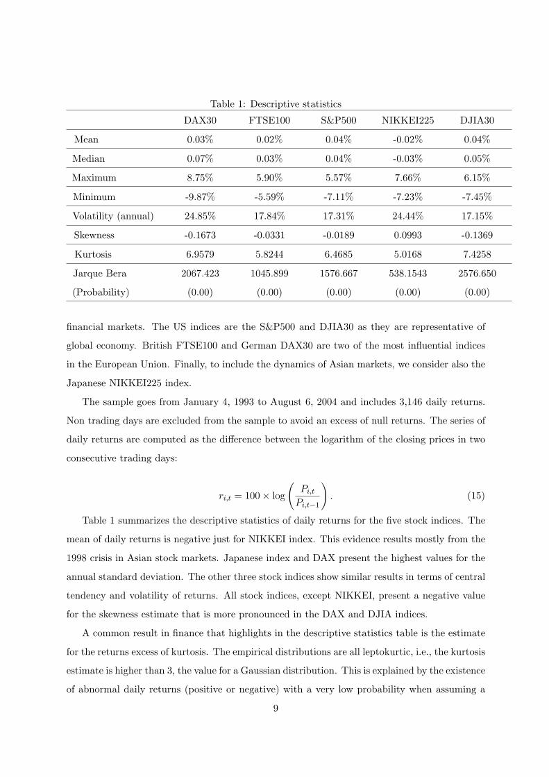
Table 1: Descriptive statistics

DAX30 FTSE100 S&P500 NIKKEI225 DJIA30

Mean 0.03% 0.02% 0.04% -0.02% 0.04%

Median 0.07% 0.03% 0.04% -0.03% 0.05%

Maximum 8.75% 5.90% 5.57% 7.66% 6.15%

Minimum -9.87% -5.59% -7.11% -7.23% -7.45%

Volatility (annual) 24.85% 17.84% 17.31% 24.44% 17.15%

Skewness -0.1673 -0.0331 -0.0189 0.0993 -0.1369

Kurtosis 6.9579 5.8244 6.4685 5.0168 7.4258

Jarque Bera 2067.423 1045.899 1576.667 538.1543 2576.650

(Probability) (0.00) (0.00) (0.00) (0.00) (0.00)

financial markets. The US indices are the S&P500 and DJIA30 as they are representative of

global economy. British FTSE100 and German DAX30 are two of the most influential indices

in the European Union. Finally, to include the dynamics of Asian markets, we consider also the

Japanese NIKKEI225 index.

The sample goes from January 4, 1993 to August 6, 2004 and includes 3,146 daily returns.

Non trading days are excluded from the sample to avoid an excess of null returns. The series of

daily returns are computed as the difference between the logarithm of the closing prices in two

consecutive trading days:

ri,t = 100× log

(Pi,t

Pi,t−1

). (15)

Table 1 summarizes the descriptive statistics of daily returns for the five stock indices. The

mean of daily returns is negative just for NIKKEI index. This evidence results mostly from the

1998 crisis in Asian stock markets. Japanese index and DAX present the highest values for the

annual standard deviation. The other three stock indices show similar results in terms of central

tendency and volatility of returns. All stock indices, except NIKKEI, present a negative value

for the skewness estimate that is more pronounced in the DAX and DJIA indices.

A common result in finance that highlights in the descriptive statistics table is the estimate

for the returns excess of kurtosis. The empirical distributions are all leptokurtic, i.e., the kurtosis

estimate is higher than 3, the value for a Gaussian distribution. This is explained by the existence

of abnormal daily returns (positive or negative) with a very low probability when assuming a

9

normal distribution. In addition, the Jarque-Bera test clearly rejects the null hypothesis of

returns normality for the five stock indices, a common result in empirical finance. Thus, normal

distribution seems not appropriate to model the indices returns and in this study we adopt a

standard Student’s t distribution for the model’s innovations to capture the observed excess of

kurtosis. The multivariate version of the standard normal density and the standard Student’s t

density are as follows:

f(ut|Ψt−1) =N√2πHt

eu′tH

−1t ut (16)

f(ut|Ψt−1) =Γ(v+N

2 )(√

π)NΓ(v2 )

(√

v)−N |Ht|−12 [1 +

u′tH

−1t ut

v]−

v+N2 . (17)

As one can see, only the standard Student’s t distribution includes a parameter (v) to describe

the tail thickness or the excess of kurtosis of returns empirical distributions.

3.2 Model Estimation

After the model’s specification, we proceed with the parameters’ estimation. We derived the log

likelihood function in order to estimate the parameters. First, it was assumed that innovations

are normally distributed (Model 1) and second, it is assumed that innovations follow a Student’s

t distribution with v degrees of freedom (Model 2).

The likelihood function for the two models are as follows:

L =t∏

i=1

f(ui|Ψi−1), (18)

where f(ui|Ψi−1) represents the density for innovations and the resulting log-likelihood functions

are:

ln = −12[p log(2π) + log |Ht|+ u′tH

−1t ut] (19)

lt = log[Γ(v + N

2)]−N

2log(π)− log[Γ(

v

2)]−N

2log(v−2)− 1

2log |Ht|− v + N

2log(1+

u′tH−1t ut

v − 2),

(20)

where |Ht| is the determinant of the conditional covariance matrix, H−1t is the inverse matrix,

v represents the degrees of freedom in the Student’s t distribution, Γ(.) is the gamma function

and N represents the number of series in the multivariate distribution.

10

To estimate the unknown parameters the previous functions need to be maximized. We use

the Marquardt algorithm in the maximization process and the estimation details are clarified

next. First, initial values are needed to start the algorithm. For the BEKK model with normal

distributed innovations, we use the returns unconditional variances and covariances for the five

stock indices, resulting in the initial covariance matrix. The initial values for diagonal elements

of matrices C∗, A∗ and G∗ were obtained by estimating five univariate GARCH(1,1) models for

the conditional variance:

σ2i,t = αi,0 + αiu

2i,t−1 + βiσ

2i,t−1. (21)

As the BEKK specification is expressed in quadratic forms, we computed the square root

of the estimates for the parameters of the univariate GARCH models in order to get the initial

values for the diagonal elements of those matrices. The general expressions for the initial values

are:

C∗ii =

√αi,0 (22)

A∗ii =√

αi (23)

G∗ii =

√βi (24)

The outer diagonal elements of the matrices were assumed to be zero at the beginning of the

algorithm.

C∗ij = A∗ij = G∗

ij = 0, where i 6= j. (25)

The starting values for the algorithm, when it is assumed that innovations follow a Student’s

t distribution with v degrees of freedom are the ones obtained from the estimation of Model 1.

Furthermore, we assume v = 3 as the initial value for this parameter. The value 3 is not without

sense. In fact, it is the minimum value for the degrees of freedom in order to assure the existence

of the second moments of the distributions. Furthermore, the estimated values resulting from

the model with Student’s t distribution were used as starting values of the models where the

leverage parameter is included.

Finally, all the estimation procedure was performed in the statistical package EViews 4.0

under 1E − 05 as the convergence criteria.

4 Estimation Results

According to our main objectives, four models have been estimated:

11

• Multivariate BEKK model with normal innovations (Model 1);

• Multivariate BEKK model with Student’s t innovations (Model 2);

• Multivariate BEKK model with Student’s t innovations and single leverage effect (Model

3);

• Multivariate BEKK model with Student’s t innovations and differentiated leverage effect

(Model 4).

Table 2 presents the maximum log likelihood value and the information criteria statistics,

resulting from the estimated models. The number of the estimated coefficients that are statis-

tically significant and the degrees of freedom estimates are also presented.

Table 2: Estimation resultsModel 1 Model 2 Model 3 Model 4

Log likelihood 67,115.20 67,459.61 67,464.43 67,490.72

Akaike Info Criterion -42.636 -42.854 -42.857 -42.871

Schwarz Criterion -42.501 -42.718 -42.718 -42.725

Number of Parameters 70 71 72 76

Significant parameters 34 29 24 29

Degrees of Freedom - 10.09 9.91 10.56

Estimation time (minutes) 66.1 172.4 74.4 145.5

The results show that the best in-sample distribution to model the innovations is the Stu-

dent’s t, according to the information criteria and the maximum log likelihood value. This is

not surprising as most of empirical studies agree that, according to the abnormal kurtosis ob-

served in financial returns series, the Student’s t distribution is more appropriate to model the

innovations conditional distribution when compared to the normal distribution.

Model 4 is the best according to the information criteria statistics. It parameterizes the con-

ditional covariance matrix including a differentiated leverage effect in the conditional variances

equations for each one of the five stock indices. It is important to observe that a higher level

of complexity, in terms of extra parameters, tends to produce a higher maximum log likelihood

value and better information criteria statistics. The three estimated models under the assump-

tion of Student’s t innovations show very similar results for the degrees of freedom estimates.

12

As one can see, the number of estimated coefficients that are statistically significant reduces

as additional features of financial returns are modeled. We can explain this by assuming that

the significance of some estimated coefficients in Model 1 results from the absence of an extra

parameter to model fat tails and the significance of some estimated coefficients in model 2 result

from the absence of the leverage effect. With the introduction of extra parameters to model

the abnormal kurtosis (v) and the leverage effects, those parameters are no longer statistically

significant.

Next, we will discuss some of the estimation results.

4.1 Multivariate BEKK model with normal innovations

Table 6 presents the estimates for the parameters in model 1. As it was referred before, only

coefficients statistically significant at the 0.05 level are reported.

TABLE 6 SOMEWHERE HERE

The first remark is that all coefficients concerning GARCH component are highly significant

and they have the expected sign. In addition, all coefficients aii and gii are positive and, for all

cases aii + gii < 1, but very near the unit.

The estimated results show evidence of strong interaction among the five stock indices returns

volatility. In fact, all conditional variances depend on factors other than the domestic ones. The

DAX conditional volatility is directly and indirectly influenced by the volatility of the FTSE

index. On the other hand, the conditional variance of the FTSE index is influenced by the

DAX squared residuals. The both countries European Union integration is one of the possible

explanations for the common dynamics of volatility in both DAX and FTSE indices. Moreover,

DAX volatility is directly and indirectly influenced by S&P500 volatility. The indirect effect of

S&P500 on DAX volatility results from the conditional covariance between FTSE and S&P500.

Note that FTSE conditional volatility is not influenced by S&P500.

The conditional volatility of S&P500 is directly and indirectly influenced by the conditional

volatility on DAX and FTSE. Note that S&P500 opens later than FTSE and DAX indices and

some of the influences on S&P500 may result from this intraday time lag. However, the intraday

dynamics on volatility is not the subject of our study.

The Nikkei index is the most independent of the five stock indices because, apart of the

13

univariate GARCH component, its conditional variance is affected only by the squared residuals

of the DAX index obtained from the conditional mean equation. Again, geographic aspects

assume some relevance, since the NIKKEI index is the most distant from the five.

Furthermore, the DJIA30 seems to be the most interdepent index as the conditional variance

is directly and indirectly influenced by all the five indices in this study. Thus, the information

from the conditional volatility of the other four stock indices impacts on DJIA30 conditional

volatility.

Model 1 shows that the most important bidirectional relationships between the stock indices

includes DAX, FTSE and S&P500. NIKKEI seems to be the least influenced, while DJIA30

is the index that incorporates more information from conditional volatilities of the other stock

indices.

Multivariate BEKK model with Student’s t innovations

Model 2 presents the same specification of Model 1. However, we now assume that the innova-

tions follow a Student’s t distribution instead of a normal distribution (table 7). As in model 1,

all coefficients concerning GARCH component are highly significant.


In Model 2 the relationship between DAX and FTSE is still valid. DAX volatility is directly

and indirectly affected by FTSE volatility and FTSE volatility is influenced by squared residuals

of the DAX returns regression. However, according to the resulting estimates for the coefficients,

this common dynamics is not so statistically relevant in this model.

On the other hand, DAX volatility is no longer influenced by the conditional volatility of

S&P500 index. The bidirectionality observed in model 1 between DAX and S&P500 does not

exist in Model 2. Furthermore, despite the maintenance of the effect of DAX and FTSE volatility

on S&P500 volatility, this influence is less strong. One possible explanation is the absence of

parameters that models the excess of kurtosis in model 1. In model 2, the excess of kurtosis is

incorporated through the parameter v, instead of possibly being implied in the estimates of the

other parameters.

The DJIA30 is still the most influenced index but the S&P500 conditional volatility no

longer affects the conditional volatility of DJIA30. In fact, S&P500 is the only one that does

14

not influence the conditional volatility of DJIA30.

According to the Student’s t specification, the NIKKEI index is also the most independent

index in terms of conditional volatility. In fact, the conditional variance of the Nikkei index

is modeled as an univariate GARCH model, with α0 = 0.0000055, α1 = 0.0457639 and β1 =

0.9269838.

The estimated value for the shape parameter is 10.09.

Modeling volatility under model 2 specification shows that there is a common dynamics in

stock market volatilities. However, this dynamics is not so strong as the one detected by model

1 does no account for the leptokurtic behavior of returns.

Multivariate BEKK model with Student’s t innovations and single leverage effect

The leptokurtosis has been taken into account in model 2 through the Student’s t distribution.

In model 3 we introduced a new parameter that represents the news asymmetric effect on volatil-

ity. As in the previous models, all the estimated coefficients concerning GARCH component are

highly significant and they are within the theoretical range.


The most important remark in this model refers to the leverage effect estimate: l = 0.0000805,

it is statistically significant at 0.05 and positive. Thus, the leverage effect exist: ”bad” news

and ”good” news have a different impact on volatility. The estimate for this parameter implies

that a negative shock in anyone of the five indices produces a higher impact on conditional

volatility than positive ones. Also, with the introduction of the leverage parameter, the number

of significant estimates reduces, particularly in terms of the parameters related to the square

residuals and cross residuals of the conditional mean equation. In fact, only the FTSE index

presents significant estimates related with the squared residuals from the other indices.

Despite the introduction of the leverage effect on volatility, the common dynamics between

DAX and FTSE still remains. S&P500 conditional variance continues to be directly and indi-

rectly influenced by the conditional volatilities of DAX and FTSE indices.

NIKKEI index maintains the specification of a univariate GARCH (1,1) model but the

conditional variance includes now a leverage effect on volatility. Therefore, the NIKKEI index

is not as independent from other stock indices as in the previous estimated models.

15

Regarding the DJIA30 index, the dynamics of conditional volatility is directly and indirectly

influenced by the conditional volatility of DAX and FTSE indices. In fact, NIKKEI and S&P500

volatilities does not influence DJIA30 volatility directly. The influence of these two stock indices

results from the leverage estimate.

Multivariate BEKK Model with Student’s t innovations and differentiated leverage

effect

Model 4 estimation results are presented in the table 9. This model introduces a differentiation

in the leverage parameter. According to the maximum log likelihood value and the information

criteria statistics, it is the most appropriated to model the dynamics of conditional covariance

matrix.


According to this specification, FTSE conditional volatility maintains the influence from the

squared residuals of DAX conditional mean. On the other hand, FTSE volatility influences the

conditional volatility of S&P500 and DJIA30 indices. However, the interactions among stock

indices resume to this.

The dynamics of volatility is implied by the leverage estimates. In our opinion, one of the

most relevant aspects of model 4 is the significance of the leverage estimate l4 = 0.008326 that

corresponds to the asymmetric effect on the NIKKEI’s conditional volatility. In fact, in the

previous models NIKKEI was the most independent index. However, model 4 shows a very

different conclusion: NIKKEI index is highly influenced by ”bad” news from other markets.

Thus, the conditional volatility in the Japanese stock index is sensitive to drops in other stock

index returns. This asymmetric behavior is very important to understand the real dynamics in

conditional variances.

The leverage estimate is also significant for the FTSE and DJIA30 stock indices. In contrary,

DAX and S&P500 indices do not present a statistically significant leverage effect.

Common sense leads investors to a market based on its liquidity and development level.

However, investors keep the other stock markets under observation. ”bad” news in one market

will certainly affect returns in the market that they are investing in. Therefore, they overreact

leading to an increase in volatility. On the other hand, ”good” news have less impact on volatility

16

because the overreaction is much lower. However, because of their level of development and

liquidity, some stock indices give investors big security. First, because of their liquidity, it is

easier for investor to redraw their investments with lower liquidity loss. Second, because of their

level of development, these indices are less influenced by the bad news of the other markets.

According to our model and assuming the previous assumptions, NIKKEI index is the most

sensitive to ”bad” news in the others markets. Note that despite the significance of the leverage

estimate of DJIA30 index, the value is close to 0, which means that there is a leverage effect

but it has a less impact in increasing the volatility.

Dynamics Correlations

Multivariate GARCH models allow to model the conditional variances and covariances. The

BEKK(1,1,1) formulation models conditional covariance in the same way as conditional vari-

ances. This means that conditional covariances are not constant over time, and depend on all

possible past variances and covariances, square residuals and cross residuals.

The following comments are based on model 4 as it has proven to be the most appropriate

model to specify the conditional covariance matrix.

The correlations between stock indices were obtained with the usual correlations formula:

ρij =Hij√

Hii×√Hjj(26)

Where ρij represents the correlation between index i and index j and Hij refers to the

relative position on the conditional covariance matrix. The correlations between two indices is

comprised between -1 and 1.

The level of correlation between financial returns and particularly between stock indices is the

most important information in order to define correct hedging strategies. Also, the estimation

of Value-at-Risk (VaR) depends from the covariances and, thereby, the correlations.

The first important thing to note is that correlations are not constant over time. The

following tables present the average correlation matrix for 3 different periods.

Correlations between the five stock indices have been increasing over time. In fact, based

on these results, the correlations show a growing trend, with a higher level of integration and

co-movement. Also, the average correlation for all the indices are positive for the three periods,

and there is the general idea of indices co-movements.

17

Table 3: Average Correlation Matrix 1991 - 1996DAX FTSE S&P500 NIKKEI DJIA30

DAX 1

FTSE 0,523 1

S&P500 0,191 0,327 1

NIKKEI 0,062 0,119 0,204 1

DJIA30 0,209 0,327 0,922 0,188 1

Table 4: Average Correlation Matrix 1997 - 2000DAX FTSE S&P500 NIKKEI DJIA30

DAX 1

FTSE 0,669 1

S&P500 0,448 0,432 1

NIKKEI 0,206 0,211 0,323 1

DJIA30 0,439 0,416 0,925 0,284 1

The most integrated stock indices are the S&P500 and the DJIA30. These two stock indices

present correlations very close to the unit in the three periods. Once again, the level of proximity

between the two indices (US indices) and the fact that the composition of S&P500 includes

securities that are also in the DJIA30 index, explains this high level of conditional correlation.

On the other hand, the NIKKEI225 index presents the lowest correlation with all the other

stock indices. In the conditional variances formulations, this index shows the lowest level of

integration with other stock indices, and this low average correlation is not surprising at all. As

proven before, the co-movement between NIKKEI225 and other indices results from the leverage

effect. However, the level of correlation with the rest of the indices has been increasing over

time.

DAX and FTSE show a significant level of correlation for the period between 1997 and

August 2004. The increasing integration of these stock indices results from the development of

the European Union, among other factors, despite the two stock indices still having two different

currencies.

Finally, S&P500 index presents one of the highest increases for the average correlations in

the three periods. This tends to demonstrate the growing importance of this stock index in the

integrated stock markets. The average correlation with the European Stock indices is about

0.5. Also, in the three periods, the S&P500 index presents the highest correlation with the

18

Table 5: Average Correlation Matrix 2001 - August 2004DAX FTSE S&P500 NIKKEI DJIA30

DAX 1

FTSE 0,712 1

S&P500 0,603 0,491 1

NIKKEI 0,282 0,245 0,358 1

DJIA30 0,589 0,487 0,958 0,332 1

NIKKEI225 index.

5 Conclusions and final remarks

The main purpose of this paper was to analyze the relationships in the returns conditional

volatilities of five stock indices: S&P500, DJIA30, FTSE100, DX30 and NIKKEI225. We have

used a multivariate variant of ARCH type models, the BEKK model (Engle and Krone, 1995)

with a multivariate leverage addition, to estimate the conditional covariance matrices. The mul-

tivariate leverage addition corresponds to a simple multivariate generalization of the univariate

GJR model. As the returns empirical distributions tend to be leptokurtic, we considered also a

standard multivariate Student’s t distribution to model innovations. According to the informa-

tion criteria statistics, this distribution has proven to be more adequate than the model normal

distribution.

Furthermore, a higher model’s generalization, under different leverage effects, brings bet-

ter results in terms of information criteria. In fact, based on the suggested parametrization,

the differentiated leverage model with Student’s t innovations provides the smallest value for

information criteria and the highest log likelihood value.

Based on estimated results, the five stock indices show some interaction in the conditional

variances and, based on the dynamics correlations, demonstrate a high level of integration that

increased with time. However, for some stock indices, namely the NIKKEI225, the interaction

results mainly from the leverage effect. Moreover, the direct and linear interaction between

stock indices decreases with the introduction: first, the Student’s t distribution and second, with

the introduction of the leverage effects. In fact, the statistical significance of some estimated

coefficients under the assumption of normality may result from the lack of parameters to model

the heavy tails and the asymmetric effect on volatility.

19

The main results present a relevant level of interaction between DAX30 and FTSE100 indices

through the estimated models. Also, the DJIA30 presents the highest level of information from

other indices; this means, for instance, that in the Student’s t innovations model, the DJIA30

conditional volatility is directly and indirectly influenced by most of the other stock indices.

Furthermore, the level of information reduces with the introduction of the leverage effect.

The leverage effect was introduced in two steps, but always under the assumption of t-

distributed innovations. First, we assume that the leverage effect is the same for all the stock

indices. The main advantage is that this allows the introduction of a leverage effect with only

one extra parameter. However, the dynamics of the asymmetry is very reduced and does not

allow the analysis of different asymmetric effects present on the five stock markets.

Therefore, we introduced a differentiated leverage effect. With this new formulation, we

assumed that different stock markets are influenced by different levels of asymmetry. The higher

degree of flexibility results in a higher number of parameters. However, this models proves to

be the most adequate parametrization for the conditional covariance matrix.

The differentiated leverage model shows a significant level of asymmetry in three indexes

(FTSE, NIKKEI and DJ30). The high level of development and liquidity of DAX and SP500

show that German and US markets are not affected by the bad news from the other markets4.

From the five stock indexes, NIKKEI presents a higher level of asymmetry within the other

indexes.

In order to fully analyze the asymmetric properties of conditional volatility, it was necessary

to introduce a new level of differentiation on the model. For so, we introduced a differential

leverage effect for each stock market. However, we assumed that in one market, investors react

in the same way to bad news whether the news come from any of the five markets, including

their how. In fact, despite the flexibility introduced by the proposed leverage effect, we assume

that investors react in the same way; either bad news comes from other stock markets or comes

from the domestic market. Furthermore, in our formulation, we did not assume there was

any currency risk. The model was parameterized under the assumption that investors have a

currency risk hedging strategy.4Note that this does not mean that there is no internal leverage effect.

20

References

[1] Black, F., 1976, Studies of stock price volatility changes. Proceedings of the 1976 Meetings

of the Business and Economics Statistics Section. American Statistical Association, 177-181.

[2] Bollerslev, Tim, 1986, Generalized Autoregressive Conditional Heteroskedasticity, Journal

of Econometrics, 31, 307-327.

[3] Bollerslev, Tim, 1987, A conditional heteroskedastic time series model for speculative prices

and rates of return, The Review of Economics and Statistics.

[4] Bollerslev, Tim, 1990, Modelling the Coherence in Short-Run Nominal Exchange Rates: A

Multivariate Generalized ARCH Model, Review of Economics and Statistics, 72: 498-505.

[5] Bollerslev, Tim; Engle, Robert; Wooldrigde, Jeffrey, 1988, A Capital Asset Pricing Model

with Time-Variyng Covariances, Journal of Political Economy, 96/1: 116-131.

[6] Engle, Robert, 1982, Autoregressive Conditional Heteroscedaticity with Estimates of the

Variance of United Kingdom Inflation, Econometrica, 50/4: 987-1006.

[7] Engle, Robert, 2002, New Frontiers for ARCH Models, Journal of Applied Econometrics

17, 425-446.

[8] Engle, Robert; Kroner, Kenneth, 1995, Multivariate Simultaneous Generalized ARCH,

Econometric Theory 11: 122-150

[9] Engle, Robert; Ng, Victor K.; Rosthschild, Michael,1990, Asset Pricing with a FACTOR-

ARCH Covariance Structure: Empirical Estimates for Treasury Bills, Journal of Econo-

metrics, 45: 213-237.

[10] Hafne, Christin M and Herwartz, Helmut, 1998, Volatility Impulse Response Function for

Multivariate GARCH Models, CORE Discussion Paper 9847.

[11] Nelson, Daniel, 1991, Conditional Heteroskedasticity in Asset Returns: A New Approach,

Econometrica, 59/2: 347-370.

[12] Silvennoinen, A. and Terasvirta, T., 2007, Multivariate GARCH models, SSE/EFI Working

Paper series in Economics and Finance, No. 669.

21

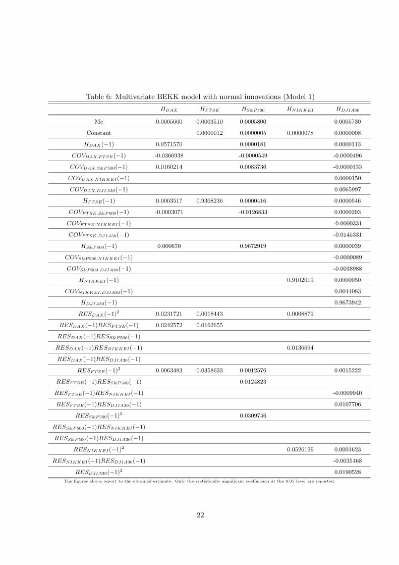
Table 6: Multivariate BEKK model with normal innovations (Model 1)

HDAX HFTSE HS&P500 HNIKKEI HDJIA30

Mc 0.0005660 0.0003510 0.0005800 0.0005730

Constant 0.0000012 0.0000005 0.0000078 0.0000008

HDAX(−1) 0.9571570 0.0000181 0.0000113

COVDAX.FTSE(−1) -0.0366938 -0.0000549 -0.0000496

COVDAX.S&P500(−1) 0.0160214 0.0083736 -0.0000133

COVDAX.NIKKEI(−1) 0.0000150

COVDAX.DJIA30(−1) 0.0065997

HFTSE(−1) 0.0003517 0.9308236 0.0000416 0.0000546

COVFTSE.S&P500(−1) -0.0003071 -0.0126833 0.0000293

COVFTSE.NIKKEI(−1) -0.0000331

COVFTSE.DJIA30(−1) -0.0145331

HS&P500(−1) 0.000670 0.9672919 0.0000039

COVS&P500.NIKKEI(−1) -0.0000089

COVS&P500.DJIA30(−1) -0.0038988

HNIKKEI(−1) 0.9102019 0.0000050

COVNIKKEI.DJIA30(−1) 0.0044083

HDJIA30(−1) 0.9673942

RESDAX(−1)2 0.0231721 0.0018443 0.0008879

RESDAX(−1)RESFTSE(−1) 0.0242572 0.0162655

RESDAX(−1)RESS&P500(−1)

RESDAX(−1)RESNIKKEI(−1) 0.0136694

RESDAX(−1)RESDJIA30(−1)

RESFTSE(−1)2 0.0063483 0.0358633 0.0012576 0.0015222

RESFTSE(−1)RESS&P500(−1) 0.0124823

RESFTSE(−1)RESNIKKEI(−1) -0.0009940

RESFTSE(−1)RESDJIA30(−1) 0.0107706

RESS&P500(−1)2 0.0309746

RESS&P500(−1)RESNIKKEI(−1)

RESS&P500(−1)RESDJIA30(−1)

RESNIKKEI(−1)2 0.0526129 0.0001623

RESNIKKEI(−1)RESDJIA30(−1) -0.0035168

RESDJIA30(−1)2 0.0190528

The figures above report to the obtained estimate. Only the statistically significant coefficients at the 0.05 level are reported.

22

Table 7: Multivariate BEKK model with t-student innovations (Model 2)


Mc 0.0006950 0.0004420 0.0006300 0.0006070

Constant 0.0000004 0.0000055 0.0000006

HDAX(−1) 0.9605490 0.0000135 0.0000083

COVDAX.FTSE(−1) -0.0226652 -0.0000423 -0.0000351

COVDAX.S&P500(−1) 0.0072459

COVDAX.NIKKEI(−1) 0.0964946

COVDAX.DJIA30(−1) 0.0056729

HFTSE(−1) 0.0001337 0.9474959 0.0000332 0.0000373

COVFTSE.S&P500(−1) -0.0113599

COVFTSE.NIKKEI(−1) -0.0000205

COVFTSE.DJIA30(−1) -0.0120438

HS&P500(−1) 0.9724011

COVS&P500.NIKKEI(−1)

COVS&P500.DJIA30(−1)

HNIKKEI(−1) 0.9269838 0.0000028

COVNIKKEI.DJIA30(−1) 0.0033067

HDJIA30(−1) 0.9720008

RESDAX(−1)2 0.0281079 0.0014491

RESDAX(−1)RESFTSE(−1) 0.113859


RESDAX(−1)RESNIKKEI(−1)


RESFTSE(−1)2 0.0223655 0.0006114 0.0005069

RESFTSE(−1)RESS&P500(−1) 0.0078794

RESFTSE(−1)RESNIKKEI(−1) -0.0004326

RESFTSE(−1)RESDJIA30(−1) 0.0060195

RESS&P500(−1)2 0.0253876



RESNIKKEI(−1)2 0.0457639 0.0000923

RESNIKKEI(−1)RESDJIA30(−1) -0.0025685

RESDJIA30(−1)2 0.0178698

The figures above report to the obtained estimate. Only the statistically significant coefficients at the 0,05 level are reported.

23

Table 8: Multivariate BEKK model with t-student innovations and single leverage effect (Model

3)


Mc 0.0006980 0.0004470 0.0006340 0.0006130

Constant 0.0000004 0.0000051 0.0000005

HDAX(−1) 0.9624218 0.0000121 0.0000075

COVDAX.FTSE(−1) -0.0211275 -0.0000316 -0.0000283

COVDAX.S&P500(−1) 0.0068508

COVDAX.NIKKEI(−1)

COVDAX.DJIA30(−1) 0.0054004

HFTSE(−1) 0.0001159 0.9500186 0.0000207 0.0000266

COVFTSE.S&P500(−1) -0.0089831

COVFTSE.NIKKEI(−1)

COVFTSE.DJIA30(−1) -0.0101740

HS&P500(−1) 0.9727640



HNIKKEI(−1) 0.9289644

COVNIKKEI.DJIA30(−1)

HDJIA30(−1) 0.9711472

RESDAX(−1)2 0.0274171 0.0013675





RESFTSE(−1)2 0.0211464

RESFTSE(−1)RESS&P500(−1)

RESFTSE(−1)RESNIKKEI(−1)

RESFTSE(−1)RESDJIA30(−1)

RESS&P500(−1)2 0.0234182



RESNIKKEI(−1)2 0.0453784

RESNIKKEI(−1)RESDJIA30(−1)

RESDJIA30(−1)2 0.0185346

Leverage 0.0000805 0.0000805 0.0000805 0.0000805 0.0000805


24

Table 9: Multivariate BEKK model with t-student innovations and differentiated leverage effect

(Model 4)


Mc 0.0007280 0.0004510 0.000670 0.0006140

Constant 0.0000004 0.0000047 0.0000005

HDAX(−1) 0.9583568

COVDAX.FTSE(−1)

COVDAX.S&P500(−1)

COVDAX.NIKKEI(−1)

COVDAX.DJIA30(−1)

HFTSE(−1) 0.9472545 0.0000237 0.0000211

COVFTSE.S&P500(−1) -0.0096092

COVFTSE.NIKKEI(−1)

COVFTSE.DJIA30(−1) -0.0090437

HS&P500(−1) 0.9733184



HNIKKEI(−1) 0.9185487

COVNIKKEI.DJIA30(−1)

HDJIA30(−1) 0.9701107

RESDAX(−1)2 0.0271498 0.0008532





RESFTSE(−1)2 0.018245

RESFTSE(−1)RESS&P500(−1)

RESFTSE(−1)RESNIKKEI(−1)

RESFTSE(−1)RESDJIA30(−1)

RESS&P500(−1)2 0.0250836



RESNIKKEI(−1)2 0.0431892

RESNIKKEI(−1)RESDJIA30(−1)

RESDJIA30(−1)2 0.0202621

Leverage 0.0034620 0.0083269 0.0002910


25

Documents

MODELING VOLATILITY IN INTERNATIONAL STOCK MARKETS