American Society for Quality - Northwestern Universityusers.iems.northwestern.edu/~ajit/papers/64) Data Reconciliation...American Society for Quality Data Reconciliation and Gross

American Society for Quality

Data Reconciliation and Gross Error Detection in Chemical Process NetworksAuthor(s): Ajit C. Tamhane and Richard S. H. MahSource: Technometrics, Vol. 27, No. 4 (Nov., 1985), pp. 409-422Published by: American Statistical Association and American Society for QualityStable URL: http://www.jstor.org/stable/1270208Accessed: 22/10/2010 10:13

Your use of the JSTOR archive indicates your acceptance of JSTOR's Terms and Conditions of Use, available athttp://www.jstor.org/page/info/about/policies/terms.jsp. JSTOR's Terms and Conditions of Use provides, in part, that unlessyou have obtained prior permission, you may not download an entire issue of a journal or multiple copies of articles, and youmay use content in the JSTOR archive only for your personal, non-commercial use.

Please contact the publisher regarding any further use of this work. Publisher contact information may be obtained athttp://www.jstor.org/action/showPublisher?publisherCode=astata.

Each copy of any part of a JSTOR transmission must contain the same copyright notice that appears on the screen or printedpage of such transmission.

JSTOR is a not-for-profit service that helps scholars, researchers, and students discover, use, and build upon a wide range ofcontent in a trusted digital archive. We use information technology and tools to increase productivity and facilitate new formsof scholarship. For more information about JSTOR, please contact [email protected].

American Statistical Association and American Society for Quality are collaborating with JSTOR to digitize,preserve and extend access to Technometrics.

http://www.jstor.org

http://www.jstor.org/action/showPublisher?publisherCode=astata

http://www.jstor.org/action/showPublisher?publisherCode=asq

http://www.jstor.org/stable/1270208?origin=JSTOR-pdf

http://www.jstor.org/page/info/about/policies/terms.jsp

http://www.jstor.org/action/showPublisher?publisherCode=astata

?1985 American Statistical Association and TECHNOMETRICS, NOVEMBER 1985, VOL. 27, NO. 4 the American Society for Quality Control

Data Reconciliation and Gross Error

Detection in Chemical Process Networks

Ajit C. Tamhane

Department of Industrial Engineering and Management Sciences

Technological Institute Northwestern University

Evanston, IL 60201

Richard S. H. Mah

Department of Chemical Engineering Technological Institute Northwestern University

Evanston, IL 60201

Measurements made on stream flows in a chemical process network are expected to satisfy mass and energy balance equations in the steady state. Because of the presence of random and

possibly gross errors, these balance equations are not generally satisfied. The problems of how

to reconcile the measurements so that they satisfy the constraints and how to use the reconciled values to detect gross errors are considered in this article. Reconciliation of measurements is usually based on weighted least squares estimation under constraints, and detection of gross errors is based on the residuals obtained in the reconciliation step. The constraints resulting from the network structure introduce certain identifiability problems in gross error detection. A thorough review of such methodologies proposed in the chemical engineering literature is given, and those methodologies are illustrated by examples. A number of research problems of potential interest to statisticians are outlined.

KEY WORDS: Constrained weighted least squares; Outlier detection; Nonlinear constraints; Steady state processes; Chemical engineering applications.

1. INTRODUCTION

A modern chemical plant consists of a large number of process units such as reaction vessels, dis- tillation columns, storage tanks, and so forth, which are interconnected together by a complicated network of streams. Measurements of mass flow rates, temperatures, concentrations of components, and so forth are routinely made for the purpose of process control and process performance evaluation. These measurements are expected to satisfy mass and energy balance constraints associated with the process network when the process is in a steady state. The given constraints are generally not satisfied, however, because of the presence of random and possibly gross errors (outliers) in the process data. The latter errors are due to miscalibrated or mal- functioning measuring instruments, unsuspected leaks, and so forth.

An additional difficulty is caused by the fact that not all variables are measured because of cost considerations or technical infeasibility. Therefore it is necessary to adjust the measured variables and, if possible, estimate the unmeasured variables so that they satisfy the balance constraints; this is known as the data reconciliation problem. Moreover, the adjustments in the process data should be utilized to detect

the presence of any gross errors so that suitable cor- rective actions can be taken; this is known as the gross error detection problem. These two problems have received considerable attention in the chemical engineering literature (Almasy and Szatno 1975; Crowe, Campos, and Hrymak 1983; lordache, Mah, and Tamhane 1985; Knepper and Gorman 1980; Kuehn and Davidson 1961; Madron, Veverka, and Venecek 1977; Mah, Stanley, and Downing 1976; Mah and Tamhane 1982; Murthy 1973; Nogita 1972; Reilly and Carpani 1963; Ripps 1965; Ro- magnoli and Stephanopolous 1981). For reviews of the literature, see Hlavacek (1977) and Mah (1981). Industrial applications of data reconciliation have been discussed, for instance, by Smith, Indiveri, and Byrne (1969); Ham, Cleaves, and Lawlor (1979); and Woodward (1984).

The main purpose of this article is to bring these problems to the attention of a wider circle of statisticians by presenting them in their basic essential mathematical framework with the usual assumptions made in the chemical engineering literature. We review in detail the methodologies proposed to solve these problems, illustrate them with examples, and indicate some of their practical and theoretical limi- tations. We also outline some open problems re- quiring further statistical research.

409

AJIT C. TAMHANE AND RICHARD S. H. MAH

2. PRELIMINARIES

2.1 Model and Assumptions

Throughout this article we assume that the process is in a steady state. Typically the process data are automatically sampled and recorded at regular time intervals of 1-5 minutes. We are concerned with the snapshot of the process at a given instant of time (needed for on-line process control) or alternatively some sort of a smoothed average of the measured variables over a given period of time, say 60 minutes (needed for process evaluation). In either case we denote by y: n x 1 the vector of measured variables; y would be the data vector at a given instant of time in the former case and the averaged data vector in the latter case. For convenience, we shall assume the former case.

We assume the following model:

y = q + e, (2.1)

where Tq: n x 1 is a vector of true values of the measured variables and e: n x 1 is a vector of errors. A more general linear model involving a general design matrix (not necessarily an identity matrix) does arise in a few applications (e.g., see Madron et al. 1977) and can be readily handled, but for simplicity we have restricted to the model (2.1). In absence (presence) of gross errors we assume that E(e) = 0 [E(e) = 6 : 0], where 0 is a n x 1 null vector. Let cov(e) = :, where L is a positive definite matrix. Throughout this article we assume that S is a known matrix, although in most cases in practice it would be estimated from the process data. If the process is in fact in a steady state (i.e., if Tq, 1, and the constraint (2.2) are fixed over time), this is not an unrealistic assumption, since a fairly accurate estimate of 2 can be obtained by cumulatively pooling the separate estimates computed for successive time periods. Each period must be reasonably short, as E(y) may change over longer time periods because of changes in E(e), although q may remain constant. The foregoing discussion im- plicitly assumes that the successive vectors of measurements are independent. Some difficulties that arise due to time-dependence of measurements are discussed in Section 7.

Let 4: m x 1 be a vector of true values corresponding to the unmeasured variables. The balance constraints are assumed to be of the following linear form:

measured variables, then (2.2) takes the form Bq = c. The data reconciliation problem is to find "good" estimates of 4 and q that satisfy (2.2).

2.2 Process Considerations Leading to Constraints (2.2)

We now explain how the constraints (2.2) are ar- rived at in practice. First, we note that a process network can be represented by a directed graph in which the nodes of the graph correspond to process units and junctions such as reaction vessels and storage tanks, and the arcs of the graph correspond to connecting streams or pipelines; the direction of each arc corresponds to the direction of mass flow in that stream. In a steady state, a mass balance equation for each component x node combination can be written as

input-output + generation-depletion = 0.

In a nonsteady state there will be an accumulation term on the right-hand side. Here all the quantities are measured as rates. For nodes involving no chemical reaction (i.e., no generation or depletion due to a chemical reaction) we simply have input = output for each component (assuming no losses due to leaks, etc.). If all the nodes in a process network are of nonreacting type and all the constraints involve only the total (not component) mass balance at nodes, then [AIB] corresponds to the incidence matrix of the directed graph of the process network in which the (i, j)th entry is + 1 if stream j is an input to node i, - 1 if stream j is an output from node i, and 0 if stream j is not incident to node i (1 < i < q, 1 < j < m + n). We refer to this as a pure network constraints case, which is illustrated by Example 2 in Section 2.3. Example 1 illustrates the case in which component mass balances are available but the nodes are of nonreacting type.

For a reacting type node the information on the amount of each component produced or consumed may be computed from the extent and the stoichiometric equation of the reaction. (The extent of a reaction is the degree of advancement or conversion of the reaction. Usually its rate of change, which has the units of moles per unit time, is used because other mass flows are measured as rates.) For example, in ammonia synthesis, nitrogen (N2) and hydrogen (H2) combine to form ammonia (NH3) according to the stoichiometric equation

A + Bql = c, (2.2) where A: q x m and B: q x n are known constant matrices and c: q x 1 is a known constant vector. A and B will be referred to as the balance matrices associated with the unmeasured and measured variables, respectively. Clearly, if there are no un-

N2 + 3H2-,2NH3. (2.3) Thus for the three components, N2, H2, and NH3, the coefficients in the reaction part of each mass balance equation will be -1, -3, and + 2, respectively, each multiplied by the extent of the reaction. These coefficients are known as stoichiometric coefficients,

TECHNOMETRICS, NOVEMBER 1985, VOL. 27, NO. 4

410

CHEMICAL PROCESS DATA RECONCILIATION

and they can always be written as integers because of the fact that all chemical compounds (products and reactants) contain integral numbers of different atoms and the atoms are conserved. The coefficients will be negative for reactants, positive for products, and zero for inert components. Example 3 in Section 6 deals with the ammonia synthesis reaction.

More generally, several chemical reactions may proceed simultaneously at a given node. In that case one needs to weight the stoichiometric coefficients of each reaction by the extent of that reaction. The ex- tents of the reactions are usually unmeasured variables.

Energy balances can be appended to mass balances by regarding the energy flow rate as an additional "component." At reacting nodes one must also take into account the standard enthalpy change (which may be known from thermodynamic considerations) for each reaction.

In summary, we note that detailed considerations of the process are required to arrive at the constraints. Here we have not indicated how nonlinear constraints may arise; this topic will be taken up in Section 5.

2.3 Examples

We now give two examples to illustrate the basic model.

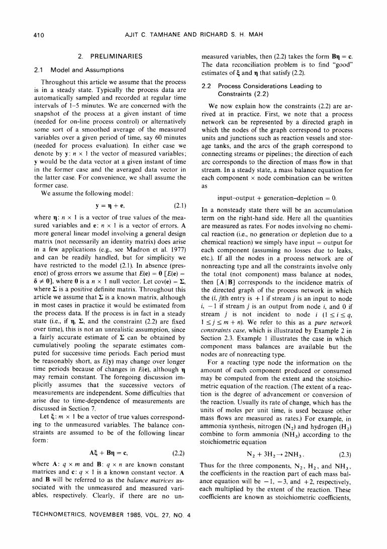
Example 1 (Ripps 1965). Consider a single- process unit with two input streams and two output streams as shown in Figure 1. Here y = (.1858, 4.7935, 1.2295, 3.8800)' is a vector of measured mass flows in the units of 1,000-pound moles per hour. No unmeasured variables are present in this example. The covariance matrix of y is assumed to be 2 = diag(2.89 x 10-4, 2.50 x 10-3, 5.76 x 10-4, 4.00 x 10-2).

There are three chemical components in each stream. The mole fractions of the components in each stream are assumed to be exactly known, and their

Table 1. Mole Fractions of Components in Different Streams

Component Stream 1 Stream 2 Stream 3 Stream 4

1 .1 .6 .2 .7 2 .8 .1 .2 .1 3 .1 .3 .6 .2

values are given in Table 1. Thus we obtain three balance equations that can be expressed in matrix form as follows:

.1 .6 -.2 -.7- o 0-

.8 .1 -.2 -.1 /2 = 0

.1 .3 -.6 -.2 ?3 0

_ 4_

where the 3 x 4 matrix on the left side is the balance matrix B and the null vector on the right side is the vector c.

We shall return to this example later.

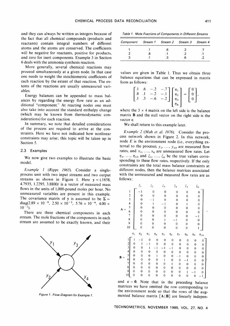
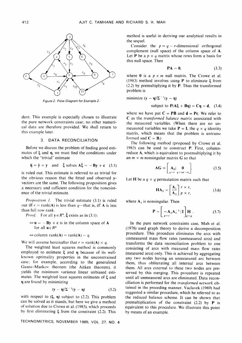
Example 2 (Mah et al. 1976). Consider the process network shown in Figure 2. In this network, node E is the environment node (i.e., everything external to the process), y ..., Ylo are measured flow rates, and xl, ..., x6 are unmeasured flow rates. Let rl, ... lo and X, ., 6 be the true values corresponding to these flow rates, respectively. If the only constraints are the total mass balance constraints at different nodes, then the balance matrices associated with the unmeasured and measured flow rates are as follows:

A

B-

1 2 3 4 5 6 7 8 9

10

i1l

1 1 2 0 3 0 4 0 5 0 6 0 7 0 8 0 9 0

10 0

-1 0 0 0 0 0 0 0 0 0

r/2

-1

0 0 0 0 0 0 0 0

0

U2

0 0

1 o 0 0 0 0 0

0

3 q/4

0 0 -1 0

1 -1

0 0 0 1 0 0 0 0 0 0 0 0 0 0

-3

0 0 0

-I 0 0 0 1 0

/5

0 0

-1 0 0 1

0 0 0 0

04

0 0 0 0 0 0 0

-1 0 0

0 0 0 0

-1 0 0 0 0 -1 0 0 1 0 0 0 0 0 0 0

05

0 0 0 1 0 0 0 0 0 0

08

0 0 0 0 0

-1

0 0 1 0

6

0 0 0 0 0 0

0 0 1

/9 r10

0 0 0 0 0 0 0 0 0 0 0 0 0 0 0 0

-1 0 0 -1

and c = 0. Note that in the preceding balance matrices we have omitted the row corresponding to the environment node so that the rows of the aug- mented balance matrix [A IB] are linearly indepen-


Figure 1 . Flow Diagram for Example 1.

411


method is useful in deriving our analytical results in the sequel.

Consider the p = q - r-dimensional orthogonal complement (null space) of the column space of A. Let P be a p x q matrix whose rows form a basis for this null space. Then

PA =0, (3.3)

Figure 2. Flow Diagram for Example 2.

dent. This example is especially chosen to illustrate the pure network constraints case; no other numeri- cal data are therefore provided. We shall return to this example later.

3. DATA RECONCILIATION

Before we discuss the problem of finding good estimates of 4 and 'q, we must find the conditions under which the "trivial" estimate

i = y = y and 4 solves A = -By + c (3.1)

is ruled out. This estimate is referred to as trivial for the obvious reason that the fitted and observed y- vectors are the same. The following proposition gives a necessary and sufficient condition for the nonexist- ence of the trivial estimate.

Proposition 1. The trivial estimate (3.1) is ruled out if r = rank(A) is less than q-that is, iff A is less than full row rank.

Proof. For all y e R", ~ exists as in (3.1):

u = -By + c is in the column space of A for all u e Rq

<column rank(A) = rank(A) = q.

We will assume hereinafter that r =- rank(A) < q. The weighted least squares method is commonly

employed to estimate 4 and q because of its well- known optimality properties in the unconstrained case; for example, according to the generalized Gauss-Markov theorem (the Aitken theorem), it yields the minimum variance linear unbiased estimates. The weighted least squares estimates of 4 and T] are found by minimizing

(y- Ti),- (y- q) (3.2) with respect to (4, tq) subject to (2.2). This problem can be solved as it stands, but here we give a method of solution due to Crowe et al. (1983), which proceeds by first eliminating 4 from the constraint (2.2). This

where 0 is a p x m null matrix. The Crowe et al. (1983) method involves using P to eliminate 4 from (2.2) by premultiplying it by P. Thus the transformed problem is

minimize (y - 'q)'- '(y - q)

subject to P(A4 + Br) = Cq = d, (3.4)

where we have put C = PB and d = Pc. We refer to C as the transformed balance matrix associated with the measured variables. (When there are no unmeasured variables we take P = I, the q x q identity matrix, which means that the problem is untrans- formed and C = B.)

The following method (proposed by Crowe et al. 1983) can be used to construct P. First, column- reduce A, which is equivalent to postmultiplying it by an m x m nonsingular matrix G so that

AG= Aol 0 . (3.5) _q x r qx(m -r)_

Let H be a q x q permutation matrix such that

HAo= A1 r x r,

A2_ P x r,

where A1 is nonsingular. Then

P= -A2A11l H . _ pxr _px p

(3.6)

(3.7)

In the pure network constraints case, Mah et al. (1976) used graph theory to derive a decomposition procedure. This procedure eliminates the arcs with unmeasured mass flow rates (unmeasured arcs) and transforms the data reconciliation problem to one consisting of arcs with measured mass flow rates (measured arcs) only. This is achieved by aggregating any two nodes having an unmeasured arc between them, thus obliterating all internal arcs between them. All arcs external to these two nodes are pre- served by this merging. This procedure is repeated until all unmeasured arcs are eliminated. Data reconciliation is performed for the transformed network obtained in the preceding manner. Vaclavek (1969) had suggested a similar procedure, which he referred to as the reduced balance scheme. It can be shown that premultiplication of the constraint (2.2) by P is equivalent to this procedure. We illustrate this point by means of an example.


412


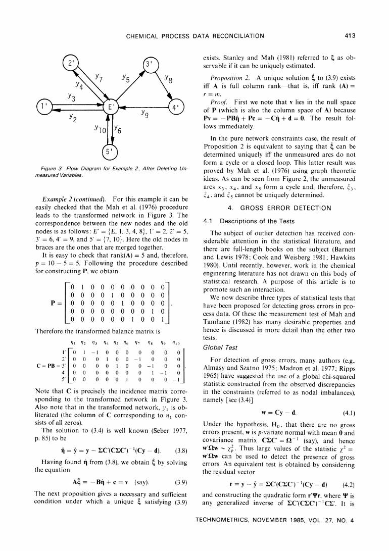
Y9

Figure 3. Flow Diagram for Example 2, After Deleting Un- measured Variables.

Example 2 (continued). For this example it can be easily checked that the Mah et al. (1976) procedure leads to the transformed network in Figure 3. The correspondence between the new nodes and the old nodes is as follows: E' = {E, 1, 3, 4, 8}, 1' = 2, 2' = 5, 3' = 6, 4' = 9, and 5' = {7, 10}. Here the old nodes in braces are the ones that are merged together.

It is easy to check that rank(A) = 5 and, therefore, p = 10 - 5 = 5. Following the procedure described for constructing P, we obtain

0 0 0 0 0

1 0 0 0 0

0 0 0 0 0

0 0 0 0 0

0 1 0 0 0

0 0 1 0 0

0 0 0 0 1

0 0 0 0 0

0 0 0 1 0

0 0 0 . 0 1

Therefore the transformed balance matrix is

71 72 73 74 75 76 77 78 79 10

1' 0 2' 0

C = PB = 3' 0 4' 0 5' 0

0 0 0 0 0

-1 0 0 0 0

0 1 0 0 0

0 0 1 0 0

0 0 0 0 1

0 -1 0 0 0

0 0

-1 1 0

0 0 0 0

0 . -1 0 0 -1

Note that C is precisely the incidence matrix corresponding to the transformed network in Figure 3. Also note that in the transformed network, yi is ob- literated (the column of C corresponding to Cl consists of all zeros).

The solution to (3.4) is well known (Seber 1977, p. 85) to be

il = y = y- 1C'(C:C')- (Cy- d). (3.8)

Having found ij from (3.8), we obtain 4 by solving the equation

A =-Bi + c = v (say). (3.9)

The next proposition gives a necessary and sufficient condition under which a unique 4 satisfying (3.9)

exists. Stanley and Mah (1981) referred to 4 as ob- servable if it can be uniquely estimated.

Proposition 2. A unique solution , to (3.9) exists iff A is full column rank-that is, iff rank (A)= r = nm.

Proof First we note that v lies in the null space of P (which is also the column space of A) because Pv = -PBi + P =-C + d = 0. The result follows immediately.

In the pure network constraints case, the result of Proposition 2 is equivalent to saying that 4 can be determined uniquely iff the unmeasured arcs do not form a cycle or a closed loop. This latter result was proved by Mah et al. (1976) using graph theoretic ideas. As can be seen from Figure 2, the unmeasured arcs x3, X4, and x5 form a cycle and, therefore, ~3,

g4, and g5 cannot be uniquely determined.

4. GROSS ERROR DETECTION

4.1 Descriptions of the Tests

The subject of outlier detection has received considerable attention in the statistical literature, and there are full-length books on the subject (Barnett and Lewis 1978; Cook and Weisberg 1981; Hawkins 1980). Until recently, however, work in the chemical engineering literature has not drawn on this body of statistical research. A purpose of this article is to promote such an interaction.

We now describe three types of statistical tests that have been proposed for detecting gross errors in process data. Of these the measurement test of Mah and Tamhane (1982) has many desirable properties and hence is discussed in more detail than the other two tests.

Global Test

For detection of gross errors, many authors (e.g., Almasy and Szatno 1975; Madron et al. 1977; Ripps 1965) have suggested the use of a global chi-squared statistic constructed from the observed discrepancies in the constraints (referred to as nodal imbalances), namely [see (3.4)]

w =Cy-d. (4.1) Under the hypothesis, Ho, that there are no gross errors present, w is p-variate normal with mean 0 and covariance matrix CIC' = f-I (say), and hence w'Tw - /z. Thus large values of the statistic 2 = w'Qw can be used to detect the presence of gross errors. An equivalent test is obtained by considering the residual vector

r = y- y = YC'(CIC') '(Cy- d) (4.2)

and constructing the quadratic form r'Tr, where v is any generalized inverse of LC'(CYC')- 1C'. It is


413


straightforward to show that w'lw = r'Vr. Note that the calculation of w and the statistics derived from it do not require that the data be reconciled first.

A difficulty with this global test is that if it indicates the presence of gross errors, then an additional testing scheme must be used to identify the sources of these errors. Ripps (1965) proposed such a scheme that has been used in slightly modified forms by other authors (Nogita 1972; Knepper and Gorman 1980; Crowe et al. 1983). In this scheme a set of s measurements (1 < s < p) suspected of containing gross errors is deleted (i.e., they are regarded as unmeasured variables with corresponding changes in the related quantities such as y, E, A, B, P, etc.) and the /2 statistic is recalculated. We would expect to get a significant reduction in x2 if the "correct" set of measurements is deleted. This can be checked by comparing the calculated x2 with a designated per- centile from the 2 distribution.

One could conceive of a scheme in which each subset of the n measurements is deleted in turn. (There are certain restrictions on the subsets of measurements that can be deleted. Clearly, the subset size cannot exceed p- 1. A further restriction is that the resulting A matrix must be full column rank according to Proposition 2.) For each subset, the Z2 statistic is calculated and its P value is assessed by referring it to the corresponding x2 distribution. (This ignores the effect of multiple testing.) The subset of measurements that upon deletion yields the least significant (having the largest P value) Z2 is then labeled as containing gross errors. It turns out, however, that such a subset may include measurements that do not contain gross errors as indicated by the significantly large x2 statistics obtained by deleting them individ- ually. On the other hand, such a subset may exclude some measurements that contain gross errors, as indicated by the significantly small /2 statistics obtained by deleting them. For an illustration of this phenomenon, see the continuation of Example 1 given at the end of this section. Therefore, usually the measurements are deleted one at a time, and those that yield significantly small x2 statistics are further tested by deleting them in groups.

For the set of measurements identified as containing gross errors, one can calculate, using (3.8) and (3.9), the adjusted vector (4, il) (where 4 includes the deleted set of measurements), which can be used for process evaluation and other purposes.

Nodal Test

Reilly and Carpani (1963) and Mah et al. (1976) independently proposed performing a separate test on each nodal imbalance (suitably standardized). Thus the test statistics are

I Zi I = I \i I /X/(C'C')ii = I wi 1/. c, (4.3)

where ci is the ith column of C (1 < i < p). These statistics can be compared against some common critical constant k. For example, one may choose k to control the familywise Type I error rate at some pre- assigned level a. If the errors ei are normally distrib- uted, then under Ho the zi are standard normal. Thus using the Sidak (1967) inequality we can choose k to be the upper a* = ?{1 -(1 - a)1P} point of the standard normal distribution.

Given a subset of significantly large nodal imbalances, Mah et al. (1976) offered an algorithm (for the pure network constraints case) for identifying those stream measurements that may contain gross errors and thus contribute to nodal imbalances. If no streams are identified as containing gross errors corresponding to a significantly large nodal imbalance, then the latter is attributed to a leak or deposition at the node that is unaccounted for in the constraint; alternatively, the constraint may have been misspecified.

Although it is possible to extend this algorithm to the case of general balance matrices, the applicability of the basic algorithm itself is limited by the assumption that the gross errors in different streams incident at a given node (i.e., either entering or leaving a given node) do not cancel out. Because of this, nodal tests are more useful as supplementary tests to verify the presence of gross errors.

Measurement Test

Since it is the measurements that contain gross errors (excluding the possibility of misspecified constraints), a more direct approach would be to base the gross error detection test on the individual residuals (also referred to as adjustments) ri. Mah and Tamhane (1982) proposed such a test. Tamhane (1982) showed that the test based on the transformed residual vector

r* = 2-lr

= C'(CEC')- (Cy -d) (4.4) has certain optimality properties for detecting the presence of a single gross error. (When L is diagonal, the tests based on r and r* are the same.) Based on this result, Mah and Tamhane (1982) recommended the use of this test for detecting gross errors, which is explained below.

First note that, under the hypothesis, Ho, that there are no gross errors present, we have

E(r*) = 0 and cov(r*) = C'QC, (4.5) where we have put nl = (CC')- '. Therefore the ith measurement can be tested for a gross error by using the statistic

=zl_ Ir*l - c'fl(Cy- d) i

/(C,'~"nc),ii x ~/' ^(4.6) i (4.6)


414


The test concludes that a gross error is present in the ith measurement iff

I zi I > k, 1 < i < n, (4.7)

where, as before, k may be chosen to be the upper C* = ?{1 - (1 - a)/n} point of the standard normal distribution.

Note that if ci is a null vector, then r* is identically zero and (4.6) cannot be calculated. However, ci = 0 does not imply that ri = 0; that is, the corresponding adjustment is not necessarily zero. The latter is true if the ith measurement is uncorrelated with all of the other measurements. We shall see an illustration of this case in the example of Section 6.

Having identified a set of measurements as containing gross errors, we can delete them and find the adjuted value (|, il) by the procedure described earlier. These adjusted values should be used in subse- quent applications.

We now point out a difficulty associated with the use of the measurement test for detecting gross errors. Suppose that the only constraint in Example 1 was the total mass balance constraint: r/ + 2 2- r/3 - 4 = 0. By substituting C = B = (1, 1, -1, -1) in (4.6) it can be checked that in that case, I z =l [Z2 = [Z3 = Z41 for all y and for arbitrary S. Thus for the given y = (Yl, Y2, Y3, y4)' and v = diag(a2, a2, a2, a2) (say), we obtain I zi = l Y~ + Y2 - Y3 Y4 I /(Z 72)1/2 = .625 for 1 < i < 4. This means that if a gross error is present, its location is nonidentifiable unless the total mass balance constraint is augmen- ted with additional information (such as the component balance constraints given in Example 1).

By working through a few simple examples, the reader can verify that this phenomenon of nonidentifiability of gross errors occurs in the pure network constraints case whenever there are two streams join- ing the same two nodes (one of which may be the environment node). In such a case the zi | statistics are identical for the two streams. The following proposition treats this problem in greater generality and gives a necessary and sufficient condition for the two I zi I statistics to have identical values.

Proposition 3. Let ci and c; be two columns of the transformed balance matrix C associated with the measured variables. Then for arbitrary 1, I zi = I zj | with probability 1 iff there exists a real constant p 0 such that pc1 = Cj-that is, iff ci and cj are collinear.

Proof. Note that I zi = I zj I for all y, and for arbitrary 1

I C'c, I/x = I C' ncj I /./Cj ncj -~:*

pc,lci = C') 0 for some p ? 0

(4.8)

From (4.8) it follows that pci = cj is a sufficient condition for zi = | Zj I to hold for all y and for arbitrary 1. To show the necessity part, suppose that pci : cj in (4.8). Then for (4.8) to hold, it must be true that the columns of C'Q = C'(CIC')-1 are linearly dependent. But this is impossible, since rank (C'Q) = p = the number of columns of C'Q. This contradiction proves the necessity part.

It can be readily checked that zi = zj (zi =-zj) for all y and for arbitary E iff p > 0 (p < 0). Thus in the pure network constraints case if two streams i and j are both inputs (from environment) to a node, then zi = Zj, and if one is input (from environment) and the other is output (to environment), then zi = -z for all y and for arbitrary L.

Note that pbi = bj for some p ?= 0 (where bi and bj are the ith and the jth columns of B, respectively) is a sufficient but not necessary condition for pci = c; to hold. In other words, even when the ith and the jth columns of the original balance matrix B are not collinear, the corresponding columns of the transformed balance matrix C can be collinear. This will happen when pbi - bj is in the null space of P (= the column space of A). See, for instance, columns for H2'1 and H{25) in matrices B and C of the example in Section 6.

In summary, to avoid the nonidentifiability problem it is necessary to incorporate enough balance constraints (usually involving additional stoichiometric information) so that no two columns are collinear. We also note that if n' (n' < n) is the number of distinct I zi I statistics, then one should choose k in (4.7) to be the upper {1- (1- _ /n"'} point of the standard normal distribution that gives a less conser- vative test.

The power of the measurement test has been stud- ied using computer simulation by lordache et al. (1985). These authors evaluated the influence of the following factors on the power of the measurement test: the magnitude of the gross error, the standard deviations of the measurements, the location of the gross error in the network, the size of the network, the balance constraints (in particular, the extent of collinearity between any two columns of the balance matrix B), and so forth. The interested reader is referred to their article for additional details.

We now return to Example 1 and illustrate the three gross error detection tests discussed in this section.

4.2 Example

Example 1 (continued). We first apply the measurement test. In this problem P = I, d = c = 0, and

.1 .6 -.2 -.7 C =B= .8 .1 -.2 -.1 .

.1 .3 -.6 -.2


415


Using (3.8) we compute y=(.1676, 4.8593, 1.1730, 3.8538)', and therefore r = y- = (-.0182, .0660, -.0565, -.0260)'. Since L is diagonal in this example, the zi statistics computed from r will be identical to those based on r* [compare (4.4)] and they are given by z = (- 1.08, 2.73, -2.62, -.13)'. Taking - = .05 we find that the upper oc* = ?{1- (.95)1 4' = .00637 point of the standard normal distribution is 2.491. We thus conclude that the second and third measurements are possibly contaminated with gross errors but not the first and fourth ones.

Next consider the global test. The Z2 statistic is 2

= r'(C'(CEC') -'C')-r = 8.455. Alternatively, the Z2 statistic can also be calculated from w= (-.0672, -.0059, -.0571)' and its covariance matrix

205.26 Q- 1 = C2C' = 29.96

_ 61.22

29.96 6.33 9.67

61.22 9.67

20.35

yielding Z2 = w'Qw = 8.455. Since this value exceeds 2L-5 = 7.815, the upper 5% point of the Z2 distribution with three degrees of freedom, presence of gross errors is indicated in the measurements.

The /2 statistics obtained by deleting Y' through y'4 (one Yi at a time) are 7.295, .964, 1.570, and 8.437, respectively. Comparing these with /2.o5 = 5.992 we find that deleting '2 or y3 yields nonsignificant x2 values, and thus gross errors may be suspected in these two measurements. We illustrate the calculation of /2 when Y2 (say) is deleted. In this case the new quantities are

.1858 .6 .1 -.2 -.7 y = 1.2295 , A= .1 , B= .8 -.2 -.1 ,

3.8800 .3 _.1 -.6 -.2

and L=diag(2.89 x 10- 4, 5.76 x 10 4, 4.00 x 10-2). From A we get

P.= 0

6 0 3 -1

and then

C =PB= -4.7 1.0 -. 1 2.3 0 -.1_'

- .03 18 w = Cy = 0393

_ .0393_' and

1- l = cL,-^ =73.60 - 27.24

-27.24

19.29_'

Finally we compute /2 = w'Q2w = .964. We may wish to confirm the result just obtained

by deleting measurements in pairs. The x2 statistics obtained by deleting ('l, Y2), (Yl, Y3) (Y,, Y4), (Y2, Y3), (Y2, 1'4), and (Y3, y4) are .552, .147, 7.273, .802, .343, and 1.440, respectively; these values may be com-

pared with 2.os5 = 3.843. It is interesting to note that the deletion of (Y2, 13) does not yield the least significant Z2, but the deletion of (yl, Y4) yields the most (and the only) significant Z2 (at a = .05). Also note that the deletion of (yl, Y3) yields the least significant Z2, although when only yi was deleted, a highly significant /2 was obtained. This illustrates the phenomenon referred to in the discussion of the global test.

In summary, using the global test, gross errors are indicated in Y2 and v'3; of course, the final decision should be made by the process engineer, taking into account all of the information available to him including the results of the gross error detection tests. By deleting '2 and y3 together we can compute the adjusted vector y = (.1722, 4.6242, 1.0201, 3.9616)' from (3.8) and (3.9).

We finally note that the three nodal test statistics [compare (4.3)] corresponding to the three constraints are .47, .24, and 1.26, all of which are nonsignificant. Thus the nodal test fails to detect the presence of gross errors in Y2 and y3. This failure of the nodal test can be explained by the fact that the gross errors in Y2 and Y3 approximately cancel out.

5. NONLINEAR CONSTRAINTS

Nonlinear constraints may arise for a variety of reasons. Typically they arise because some coefficients in the balance matrices A and B are not exactly known (e.g., as assumed in Example 1) and are either unmeasured or measured variables. This results in the corresponding constraints of (2.2) being bilinear; that is, they involve terms that are products of two unknown parameters (d's or q's). For example, consider a multicomponent stream input into a node that is split into two output streams. Then the split fraction is the same for each component. If this fraction is unknown (and hence is to be estimated from the data), then the resulting set of constraints are bilinear; see the example of Section 6 for an illustration. Another example of a bilinear constraint arises in balancing energy flow rates when the energy flow rates are not directly measured but are calculated from the products of mass flow rates and temper- ature changes, both of which may be measured. Non- linear constraints may also arise because certain variables are measured indirectly and the relationship between the variable actually measured and the variable of interest may be nonlinear. For example, con- centration may be measured via density, pH values, or thermal conductivity.

Let us replace (2.2) by q x 1 constraint vector

f(4, q) = 0, (5.1) where f= (f, f2 ... , fq)' and each fi(4, r) may be nonlinear in both 4 and qi. Knepper and Gorman


416


(1980) proposed a Gauss-Newton type iterative algorithm for estimating 4 and q. The algorithm is initiat- ed with some starting values 4(O) and q(o), where q(o) is usually taken to be the observed vector y. To find the estimates 4(i+1) and q(i+ ) at the (i + l)th stage of the algorithm, f(4(i+ l), i(i+ 1)) is approximated by a first-order (linear) Taylor series expansion around (E(i), tl()) and then equated to 0. The resulting set of equations is solved for 4(l+1) and q(i+l) by a combination of the least-squares method for 4(i+ l) and the weighted least-squares method for qii+ 1). We get the following expressions for 4(i + ) and (i + ):

~(i+ 1)_ -(i) = (G(i),Q(i)G(i))- 1G(i)Q(i)

x {-f((i), (i)0) + H(i)(li') - 1(0))} (5.2)

and

qi/+ ~) _ (O) = ,H(O,

x [I - G(')(G()'Q(')G())- G(i)'Q(')]

x {-f( (i), 1('0) + H(i)(i-(i)- rl(?))}. (5.3)

Here G('): q x m and H(/): q x n are the matrices of first partial derivatives of f with respect to 4 and iq, respectively, evaluated at (4(i), l(i)), and Q'i)= (H(i)H(/)')-1. The final estimates (4, fi) are taken to be (4(i), q(i)) when the algorithm converges. See Britt and Leucke (1973) for additional details, including the statistical properties of the estimated parameters.

Crowe et al. (1983) dealt with the special case of bilinear constraints in which some entries of A and B are unknown; these are assumed to be unmeasured. Let ': I x 1 denote the vector of these unknown entries. Thus the matrices A, B, P, and C are functions of ~. To estimate ~, Crowe et al. (1983) proposed the following method.

Let

L = (y - )'- l(y -_ l) + '(C1 - d) (5.4)

be the Lagrangian function associated with the constrained optimization problem (3.4), where ;: p x 1 is a vector of Lagrange multipliers. For some given values of 'q and X, let

aL/ac, = '[(C/S)q - (9d/C,)], 1 i < k, (5.5)

where in most cases aC/in and cd/oi v will be a constant matrix and a constant vector, respectively. The

.82 1.14 5.12E

1.14 6.34

3 1.42E

method consists of solving for q [using (3.8)] and k

using some initial estimate of g and updating that estimate by the steepest descent or the secant method [which requires the first partials (5.5)]; this scheme is iterated until convergence is reached. Crowe et al. (1983) suggested that inferences concerning gross errors be made by regarding the final estimate ~ as a fixed quantity, but the validity of this suggestion is questionable.

6. A COMPREHENSIVE EXAMPLE

Example 3 (Crowe et al. 1983). The flow diagram for ammonia synthesis is shown in Figure 4. A feed stream containing nitrogen (N2), hydrogen (H2), and argon (Ar) (an inert impurity) is mixed with the recy- cle stream 7 at node 1. The reaction according to (2.3) takes place in the reactor (node 2). The product, ammonia (NH3), is recovered in the separator (node 3), and the unreacted gases are recycled to the splitter unit (node 4), where an unknown fraction of them is purged from the system (to avoid the buildup of argon).

To make it easier to refer to the various chemical components involved, a different notation is used in the sequel. The flow rate of component A in stream i is denoted by A(i). Observed and reconciled flow rates are not denoted by separate symbols, but they are labeled accordingly in the tables to follow. The rate of change of the extent of reaction (2.3) is denoted by c. Finally, the fraction of N2, H2, and Ar purged through stream 6 is denoted by (. Both ~ and C are unmeasured variables.

The matrices A and B are given in Figures 5 and 6. Note that for each node we have a separate mass

flow balance for each component. At node 4, in addi- tion to the component mass flow balances, we have the splitter constraints, which state that the ratio of mass flow rate in stream 6 to that in stream 5 is the same for N2, H2, and Ar; this ratio is C, the fraction purged. In the sequel we shall see the effect of ignor- ing the splitter constraints on data reconciliation. Also note the stoichiometric coefficients in the last column of A, which are taken from the reaction equation (2.3).

The covariance matrix of the measured flow rates is assumed to be known and equal to

Ar(l) N(22) Ar(2) N(3) NH(4) H(5'

5.12E-3 1.42E - 4

4 1.28E - 4 8.16 .816 8.16 .326

3.81 3.08

3.20


417


Purge

1

N2 ,H2 Ar

Mixer Reactc

Figure 4. Flow Diagram for Examp

The block-diagonal nature of I comes from the assumption that the measurements in the same stream are correlated but those in different streams are uncorrelated.

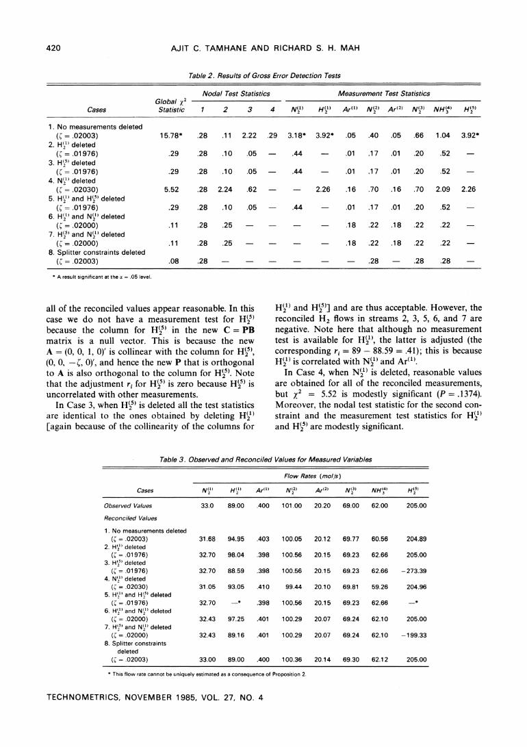
Table 2 gives the results of the tests for detection of gross errors. Table 3 gives the observed and reconciled values of the measured variables under different conditions. Table 4 gives the reconciled values of the unmeasured variables under the same conditions. Note that in Table 2 the number of nodal test statistics in each case is the difference, p, between the number of original constraints and the total number

5 N2 ,H2 ,Ar

:er

3 Separator

N2, H2

Ar,NH NH3

ammonia synthesis loop

le 3 (ammonia synthesis loop).

of unmeasured variables and deleted measurements. In this example there are 17 constraints, including the 3 splitter constraints; 13 unmeasured variables; and 0, 1, or 2 deleted measurements. All of the matrix computations were performed using standard sub- routines in the IMSL package.

The measurement tests are based on the transformed residuals, since I is not diagonal. The measurement test statistics are not computed for deleted variables and for those variables for which the corresponding columns of C are null vectors.

The significance level used for each measurement

H(2' H(3 NH33' Ar(3 N(5) Ar(5) N(26 H(6 Ar'6' N27) H27) Ar (7

-3 2

-1

Figure 5. Matrix A for Example 3.


A

N2

Node 1 H2 Ar

N2

H2 Node 2 NH3

Ar

N, H2

Node 3 NH3 Ar

N2 Node 4 H2

Ar

Splitter N2 Con- H2 straints Ar

418

1

1 -1I

- 1 1

-1

1 -1

1

1

1 - 1

1 - 1 - 1

1


N2

Node 1 H2 Ar

N2 H2

Node 2 NH3 Ar

N2 H2

Node 3 NH3 Ar

N2 Node 4 H2

Ar

Splitter N2 Con- H2 straints Ar

-1

Figure 6. Matrix B for Example 3.

test is a* = ?{(1 - (1 - )1/n'}, where n' is the number of distinct Izi statistics. Similarly, the significance level used for each nodal test is a*= {1-(1-a) /P}. The test results significant at a = .05 are indicated by asterisks. We now discuss the results in detail.

First consider Case 1, where no measured variables are deleted. By regarding ( as a known fixed quantity, we can find a projection matrix P; here we have q = 17 and r = m = 13; thus p = q - r = 4. One choice of P is

0

P= I

0 0

00 00 1 0 0 1

1 0 00 0 1 00

.5 0

1.5 0

0 0 0

1 -

of B were not collinear; this refers to the remark made in the second paragraph following Proposition 3.

The nodal test for the third constraint (refer to C given before) also gives a modestly significant result (P = .15). Note that both H2I) and H(25) enter this constraint but N() does not. Nonetheless, we shall explore the effects of deleting each one of these measurements (separately and in groups). In making

0 1 -

~

0 0

0 0 1 0

.5 0

1.5

0 0 0

1 -C

0 1 0 0

0 0 1 0

00 0 1 00 1 0

which yields

0

C = PB =I

L o

0 0 1 0

0 0 0 1

1 -1

0 0

0 0 0 -C

-1 1 -C

0 0

-.5 0

-1.5 0

00 0 0 1 0 '

0 1

o?1 o] 0

0

A simple physical interpretation can be given to the rows of C. They correspond to an elemental nitrogen balance around the reactor, the split condition for nitrogen, and the overall elemental balances on hydrogen and argon, respectively.

The unknown split fraction ( is estimated to be .02003, using the algorithm suggested by Crowe et al. (1983). In this case all three gross error tests are trig- gered. In particular, the measurement test points to H(21), H(25), and N(2') as potential culprits. Note that the measurement test statistics for H(21) and H5) are identical because the corresponding columns of C are collinear. Note also that the corresponding columns

the ensuing calculations we can replace the B matrix with the C matrix calculated before; there is no A matrix in the transformed problem. When H"2) (say) is deleted, the new A matrix is the corresponding column of the C matrix, namely, (0, 0, 1, 0)', and the new B matrix is formed by the remaining columns of the C matrix. It is then straightforward to find a new P that is orthogonal; the new A = (0, 0, 1, 0)'. Let us now look at the results obtained by deleting H21), H?), and N").

In Case 2, when H") is deleted the results of all the gross error detection tests are acceptable. Moreover,


B

419

N() H(') Ar(l) N(22) Ar(2) N(23) NH(4) H?

1 1

1 1

1 - 1

1

1

-1 1

1

N(21) H() Ar(1) N(2) Ar(2) N(3) NH(3) H5)


Table 2. Results of Gross Error Detection Tests

Nodal Test Statistics Measurement Test Statistics Global x2

Cases Statistic 1 2 3 4 N(1) H( Ar(1) N(22 Ar(2) N(3) NH() H(25

1. No measurements deleted ( = .02003) 15.78* .28 .11 2.22 .29 3.18* 3.92* .05 .40 .05 .66 1.04 3.92*

2. H(1) deleted (= .01976) .29 .28 .10 .05 - .44 - .01 .17 .01 .20 .52

3. H?( deleted (- .01976) .29 .28 .10 .05 - .44 - .01 .17 .01 .20 .52

4. N(,1) deleted ( -= .02030) 5.52 .28 2.24 .62 - 2.26 .16 .70 .16 .70 2.09 2.26

5. H(1) and H(25 deleted (= .01976) .29 .28 .10 .05 - .44 - .01 .17 .01 .20 .52 -

6. H') and N(2) deleted ( = .02000) .11 .28 .25 - - - - .18 .22 .18 .22 .22 -

7. H(5) and N(1) deleted (? = .02000) .11 .28 .25 - - - - .18 .22 .18 .22 .22

8. Splitter constraints deleted ( = .02003) .08 .28 - - - - - - .28 - .28 .28

*A result significant at the a = .05 level.

all of the reconciled values appear reasonable. In this case we do not have a measurement test for H2 because the column for H(25 in the new C = PB matrix is a null vector. This is because the new A = (0, 0, 1, 0)' is collinear with the column for H(5),

(0, 0, - C, 0)', and hence the new P that is orthogonal to A is also orthogonal to the column for H(. Note that the adjustment ri for H(25) is zero because H5) is uncorrelated with other measurements.

In Case 3, when H() is deleted all the test statistics are identical to the ones obtained by deleting H?(2' [again because of the collinearity of the columns for

H?) and H5)] and are thus acceptable. However, the reconciled H2 flows in streams 2, 3, 5, 6, and 7 are negative. Note here that although no measurement test is available for H(), the latter is adjusted (the corresponding ri = 89 - 88.59 = .41); this is because H() is correlated with N(2) and Ar"().

In Case 4, when N(1) is deleted, reasonable values are obtained for all of the reconciled measurements, but x2 = 5.52 is modestly significant (P = .1374). Moreover, the nodal test statistic for the second constraint and the measurement test statistics for H(2 and H5) are modestly significant.

Table 3. Observed and Reconciled Values for Measured Variables

Flow Rates (molls)

Cases N(21 H(21) ArM() N(22 Ar(2) N(23) NH(34) H 2')

Observed Values 33.0 89.00 .400 101.00 20.20 69.00 62.00 205.00

Reconciled Values

1. No measurements deleted ( = .02003) 31.68 94.95 .403 100.05 20.12 69.77 60.56 204.89

2. H2) deleted (C = .01976) 32.70 98.04 .398 100.56 20.15 69.23 62.66 205.00

3. H'' deleted (= .01 976) 32.70 88.59 .398 100.56 20.15 69.23 62.66 -273.39

4. NW1] deleted ( = .02030) 31.05 93.05 .410 99.44 20.10 69.81 59.26 204.96

5. H',) and H() deleted ( = .01976) 32.70 -* .398 100.56 20.15 69.23 62.66 -*

6. H`' and N2'1) deleted ( .02000) 32.43 97.25 .401 100.29 20.07 69.24 62.10 205.00

7. H'"5 and N(2' deleted ( =.02000) 32.43 89.16 .401 100.29 20.07 69.24 62.10 -199.33

8. Splitter constraints deleted

( = .02003) 33.00 89.00 .400 100.36 20.14 69.30 62.12 205.00

*This flow rate cannot be uniquely estimated as a consequence of Proposition 2.


420


Table 4. Reconciled Values for Unmeasured Variables

Flow Rates (mol/s)

Cases H(2) H(3) NH(3) Ar(3) N(5) Ar() N(6) H(6) Ar(6) N(7) H7) Ar 7)

1. No measurements deleted (C=.02003) 295.74 204.89 60.56 20.12 69.77 20.12 1.40 4.10 .40 68.37 200.79 19.72 30.28

2. H('_ deleted (C =.01976) 298.99 205.00 62.66 20.15 69.23 20.15 1.37 4.05 .40 67.86 200.95 19.75 31.33

3. H',5' deleted (.= .01976) -179.40 -273.39 62.66 20.15 69.23 20.15 1.37 -5.40 .40 67.86 -267.99 19.75 31.33

4. N I deleted ( =.02030) 293.85 204.96 59.26 20.10 69.81 20.10 1.41 4.16 .41 68.39 200.80 19.69 29.63

5. HI"2 and H5) deleted ( =.01976) * * 62.66 20.15 69.23 -* -* * * 67.86 -* 19.75 31.33

6. H'" and N(21) deleted (C=.02000) 298.15 205.00 62.10 20.07 69.24 20.07 1.38 4.10 .40 67.86 200.90 19.67 31.05

7. H(' and N,) deleted (C=.02000) -106.17 -199.33 62.10 20.07 69.24 20.07 1.38 -3.99 .40 67.86 -195.34 19.67 31.05

8. Splitter constraints deleted ( = .02003) 293.18 205.00 62.12 20.14 69.30 20.14 1.94 -4.18 .40 67.36 209.18 19.74 31.06

* This flow rate cannot be uniquely estimated as a consequence of Proposition 2.

Based on the test results thus far, we may suspect a gross error in Hi21). Cases 5, 6, and 7 give the results obtained by deleting HI2'), H125), and N"2) in pairs. We note that deleting H2) and N'2") gives acceptable results, but deleting H5) and N2)9 gives negative reconciled values for several flow rates. We also note that deleting H"2) and HI2) results in the corresponding A matrix being less than full column rank, which causes several unmeasured variables [including the deleted variables HI21) and H25)] to be not uniquely estimable; in this case there are no measurements on H2 flows and thus H2 flows are clearly not estimable. These sets of tests confirm the earlier conclusion of a gross error in HI21 and, together with the previous test results, they suggest that N"2) may also contain a gross error.

Case 8 is intended to show the effect of omitting the three splitter constraints. In that case all three gross error tests are passed and the reconciled values look reasonable except that H26) comes out negative. This case illustrates the danger of using an incom- plete constraint set. Here, since the number of constraints is reduced to 14 and there are 13 unmeasured variables, the system is almost unconstrained (the "trivial" estimate case of Theorem 1). Only slight adjustments are made in some unmeasured variables, which causes the gross error detection tests to not trigger.

7. CONCLUDING REMARKS AND DIRECTIONS FOR FUTURE RESEARCH

This review suggests a number of research problems of potential interest to statisticians. We briefly discuss some of these problems next.

1. All of the results for the steady state are given

under the assumption of known E. In practice, one must estimate E from the data. If the process is in a steady state and the successive measurement vectors are independent, then Y can be estimated without much difficulty. The consecutive observations would generally be correlated, however, and in that case it is far from clear what are good ways to estimate E. Moreover, there is the problem of modifying the data reconciliation and gross error detection procedures to account for estimated 2.

2. Another problem in the case of time-dependent observations, which has not been addressed in the literature, is how to take into account the dependence structure (typically unknown) in computing smoothed averages and using them for reconciliation and gross error detection purposes. Note that this problem is present even when E is assumed known.

3. As we have seen, in the case of linear constraints, the unmeasured variables can be readily eliminated from the constraints and a closed-form solution [compare (3.8) and (3.9)] can be obtained for the data reconciliation problem. A corresponding reduction of the problem is not available when the constraints are of general nonlinear nature. Thus ef- ficient computational methods are needed to deal with this case. Knepper and Gorman (1980) made a contribution in this direction, but the computational efficiency of their algorithm remains to be tested. Much theoretical work is also needed concerning the statistical properties of the gross error detection tests for the nonlinear case.

4. The closed-form solution to the constrained weighted least squares problem does not take into account the natural nonnegativity restrictions on the flow rates and other quantities. We saw in Example 3 that nonnegativity restrictions are crucial in a "cor-


421


rect" scheme for gross error detection. Hence one should explicitly take them into account. However, this will make the data reconciliation and gross error detection procedures considerably more complicated.

5. In practice, the failure to satisfy the balance constraints may result not only because of random and gross errors in measurements but also because of misspecifications of the constraints. It would be desirable to have a combination of measurement tests and nodal tests that would properly identify the culprits. However, this seems possible only under very restrictive assumptions (as in Mah et al. 1976).

6. Finally, we note that only the steady state processes are considered in this article. In the nonsteady state case, the Kalman filter model has been used by Stanley and Mah (1977) for the data reconciliation problem and by Newman (1982) for the gross error detection problem. However, the methodological de- velopments lag far behind compared to the steady- state case.

It is our hope that this review article will en- courage more statisticians to work on the related problem areas, including the ones suggested here.

ACKNOWLEDGMENT

We are grateful to the editor, an associate editor, and the referees for their detailed comments on the first draft of this article, which led us to considerably expand the scope of our review. We also wish to thank Corneliu lordache for computational assist- ance. The work on this article was partially support- ed by National Science Foundation Grant CPE81- 15161 at Northwestern University. The work on the first draft was performed while the first author was visiting Cornell University on sabbatical leave during 1982 and 1983 with partial support from U. S. Army Research Office (Durham) Contract DAAG-29-81-K- 0168.

[Received February 1984. Revised March 1985.]

REFERENCES

Almasy, G. A., and Szatno, T. (1975), "Checking and Correction of Measurements on the Basis of Linear System Model," Problems of Control and Infbrmation Theory, 4, 57-69.

Barnett, V., and Lewis, T. (1978), Outliers in Statistical Data, New York: John Wiley.

Britt, H. I., and Leucke, R. H. (1973), "The Estimation of Parame- ters in Nonlinear Implicit Models," Technometrics, 15, 233-247.

Cook, R. D., and Weisberg, S. (1982), Residuals and Infiuence in Regression, London: Chapman and Hall.

Crowe, C. M., Campos, Y. G., and Hrymak, A. (1983), "Reconcilia- tion of Process Flow by Matrix Projection," The American Insti- tute o. Chemical Engineers Journal, 29, 881-888.

Ham, P. G., Cleaves, G. W., and Lawlor, J. K. (1979), "Operation Data Reconciliation: An Aid to Improved Plant Performance," in Proceedings of l 1th World Petroleum Congress (Vol. 4), London: Applied Science Publishers, pp. 281-286.

Hawkins, D. M. (1980), Identification of Outliers, London: Chapman and Hall.

Hlavacek, V. (1977), "Analysis of a Complex Plant-Steady State


and Transient Behavior," Computers in Chemical Engineering, 1, 75-100.

lordache, C., Mah, R. S. H., and Tamhane, A. C. (1985), "Per- formance Studies of the Measurement Test for Detection of Gross Errors in Process Data," The American Institute of Chemi- cal Engineers Journal, 27, 1187-1201.

Knepper, J. C., and Gorman, J. W. (1980), "Statistical Analysis of Constrained Data Sets," The American Institute of Chemical Engineers Journal, 26, 260-264.

Kuehn, D. R., and Davidson, H. (1961), "Computer Control I1: Mathematics of Control," Chemical Engineering Progress, 57, No. 6,44-47.

Madron, T., Veverka, V., and Venecek, V. (1977), "Statistical Analy- sis of Material Balance of a Chemical Reactor," The American Institute of Chemical Engineers Journal, 23, 482-486.

Mah, R. S. H. (1981), "Design and Analysis of Process Performance Monitoring Systems," in Proceedings of the Engineering Founda- tion Conference on Chemical Process Control (Vol. 2), New York: Engineering Foundation, pp. 525-540.

Mah, R. S. H., Stanley, G. M., and Downing, D. M (1976), "Recon- ciliation and Rectification of Process Flow and Inventory Data," Industrial and Engineering and Chemical Process Design and De- velopment, 15, 175-183.

Mah, R. S. H., and Tamhane, A. C. (1982), "Detection of Gross Errors in Process Data," The American Institute of Chemical Engineers Journal, 28, 828-830.

Murthy, A. K. S. (1973), "A Least Squares Solution to Mass Bal- ance Around a Chemical Reactor," Industrial and Engineering Chemical Process Design and Development, 12, 246-248.

Newman, R. S. (1982), "Robustness of Kalman Filter Based Fault Detection Methods," unpublished Ph.D. dissertation, University of London.

Nogita, S. (1972), "Statistical Test and Adjustment of Process Data," Industrial and Engineering Chemical Process Design and Development, 11, 197-200.

Reilly, P. M., and Carpani, R. E. (1963), "Application of Statistical Theory of Adjustment to Material Balances," 13th Canadian Chemical Engineering Conference, Ottawa: Chemical Institute of Canada.

Ripps, D. L. (1965), "Adjustment of Experimental Data," Chemical Engineering Progress Symposium Series, 61, No. 55, 8-13.

Romagnoli, J. A., and Stephanopolous, G. (1981), "Rectification of Process Measurement Data in the Presence of Gross Errors," Chemical Engineering Science, 36, 1849-1863.

Seber, G. A. F. (1977), Liner Regression Analysis, New York: John Wiley.

Siddk, Z. (1967), "Rectangular Confidence Regions for the Means of Multivariate Normal Distributions," Journal of the American Statistical Association, 62, 626-633.

Smith, R. A., Indiveri, R. L., and Byrne, W. M. (1969), "Material Balancing Process Plant by Network Analysis," in NPRA Com- puter Conference, Washington, DC: National Petroleum Refiners Association.

Stanley, G. M., and Mah, R. S. H. (1977), "Estimation of Flows and Temperatures in Process Networks," The American Institute of Chemical Engineers Journal, 23, 642-650.

(1981), "Observability and Redundancy in Process Data Estimation," Chemical Engineering Science, 36, 259-272.

Tamhane, A. C. (1982), "A Note on the Use of Residuals for Detecting an Outlier in Linear Regression," Biometrika, 69, 488- 489.

Vaclavek, V. (1969), "Studies on System Engineering II: On the Application of the Calculus of Observations in Calculations of Chemical Engineering Systems," Collections of Czechoslovak Chemical Communications, 34, 364-372.

Woodward, J. W. (1984), "A Generalized Data Reconciliation System for Process Computer System," unpublished paper pre- sented at the American Institute of Chemical Engineers national meeting in Anaheim, Calif.

422

Documents

American Society for Quality - Northwestern Universityusers.iems.northwestern.edu/~ajit/papers/64) Data Reconciliation...American Society for Quality Data Reconciliation and Gross