Indian Statistical Institute

Ranking and Selection Problems for Normal Populations with Common Known Coefficient ofVariationAuthor(s): Ajit C. TamhaneSource: Sankhyā: The Indian Journal of Statistics, Series B, Vol. 39, No. 4 (Jun., 1978), pp.344-361Published by: Indian Statistical InstituteStable URL: http://www.jstor.org/stable/25052085Accessed: 22/10/2010 11:28

Your use of the JSTOR archive indicates your acceptance of JSTOR's Terms and Conditions of Use, available athttp://www.jstor.org/page/info/about/policies/terms.jsp. JSTOR's Terms and Conditions of Use provides, in part, that unlessyou have obtained prior permission, you may not download an entire issue of a journal or multiple copies of articles, and youmay use content in the JSTOR archive only for your personal, non-commercial use.

Please contact the publisher regarding any further use of this work. Publisher contact information may be obtained athttp://www.jstor.org/action/showPublisher?publisherCode=indstatinst.

Each copy of any part of a JSTOR transmission must contain the same copyright notice that appears on the screen or printedpage of such transmission.

JSTOR is a not-for-profit service that helps scholars, researchers, and students discover, use, and build upon a wide range ofcontent in a trusted digital archive. We use information technology and tools to increase productivity and facilitate new formsof scholarship. For more information about JSTOR, please contact support@jstor.org.

Indian Statistical Institute is collaborating with JSTOR to digitize, preserve and extend access to Sankhy: TheIndian Journal of Statistics, Series B.

http://www.jstor.org

Sankhy? : The Indian Journal of Statistics

1978, Volume 39, Series B, Pt. 4, pp. 344-361.

RANKING AND SELECTION PROBLEMS FOR NORMAL

POPULATIONS WITH COMMON KNOWN

COEFFICIENT OF VARIATION

By AJIT C. TAMHANE

Northwestern University, Evanston

SUMMARY. The problem of selecting the normal population having the largest mean

has been widely studied in the literature by treating the population means and the variances

as unrelated parameters. But it is very common in practice to find that the population standard

deviations are related to the means by a proportionality relation ; the constant of proportionality

being known as the coefficient of variation. In this paper single-stage ranking and selection

procedures are proposed for the above situation where the populations under study have a

common known coefficient of variation. The indifference-zone approach and the subset selection

approach are both considered. The large sample theory is studied in detail and the correspond

ing tables are provided for implementing the proposed procedures. The small sample theory

is discussed briefly in the Appendix.

1. Introduction

The problem of choosing the population having the largest mean where

the populations under study ?,re assumed to be normal is a very important one in practice and has received most attention in the ranking and selection

literature. In his pioneering paper, Bechhofer (1954) proposed the so-called

indifference-zone approach to this problem (referred to as the normal means

problem hereafter) and gave a single-stage procedure for the case of known

variances. For the case of unknown variances two-stage procedures were

studied by Bechhofer, Dunnett and Sobel (1954) and Dudewicz and Dalai

(1975). Another so-called subset selection approach to the normal means

problem was proposed by Gupta (1956 and 1965) who gave single-stage

procedures for the cases of common known variance and common unknown

variance (see also Gupta and Sobel, 1957). Recent reviews of the literature on

the normal means problem may be found in Wetherill and Ofosu (1974) and

Bechhofer (1975).

All of the work on the normal means problem so far assumed that the

population means and the variances a,re unrelated parameters. However,

in practice, as Gleser and Healy (1976) recently pointed out, it is common to

find, particularly in physical and biological applications, that the population standard deviations are proportional to their means; the constant of

proportionality being known as the coefficient of variation. In such a situation

SELECTION PROBLEMS FOR NORMAL POPULATIONS 345

where the population means and the variances may be assumed to be related

parameters, the procedures those have been developed for the case of unknown

variances would be inappropriate. The knowledge of the proportionality relation between the population means and the standard deviations should

be used to develop new ranking and selection procedures. This is the purpose of the present paper.

In particular we propose single-stage procedures (for two different goals) which use estimators developed by Gleser and Healy (1976) for the case where

the coefficient of variation is known to the experimenter. This would be

a reasonable assumption in practice if the data from past experiments dealing with similar populations (e.g., yield data about similar varieties of a grain from the records of previous field trials) are available which would enable

a fairly accurate estimate of the coefficient of variation to be obtained from

the scatterplots of the sample means and the sample standard deviations.

The case of unknowTn coefficient of variation cannot be handled by a single

stage procedure (at least for the goal employing the indifference-zone approach) ; this problem is under study at present.

The statistical formulation of the problem is given in Section 2. In

Section 3 we discuss the choice of the estimator for the means to be used in

our procedures. We then point out certain difficulties associated with the

practical implementation of the exact small sample results for the selected

estimators and how these difficulties may be overcome using the large sample

theory. In Section 4 we give large sample results for the procedures which

use any best asymptotically normal (B.A.N) estimator for the means. The

adequacy of the large sample approximation is investigated by a simulation

study and it is found that the large sample approximation is quite good but

little bit on the deficient side. The tables for implementing the procedures in the large sample case are given at the end of the paper. These tables are

related to the tables of the equi-correlated multivariate normal distribution

published by Gupta, Nagel and Panchapakesan (1973) and, therefore, they have additional applications as discussed by these authors. Finally we give some concluding remarks in Section 5.

2. Preliminaries

2.1. Assumptions and notation. Let m (1 <; i ̂ k) denote a normal

population with unknown mean 0t and variance ocdf where a > 0 is assumed

to be known. As explained in Gleser and Healy (1976) we shall assume, without

loss of generality, that the coefficient of variation \/ot and the means

0?(1 ^ * ̂ k) are positive constants. Let d^t] ̂ 6[2] ̂ ... ^ 0[fcj be the

346 A JIT C. TAMHANE

ordered values of the means. We shall assume that the experimenter has no

prior knowledge concerning the correct pairing between 77^ and 6^ (1 ̂ i, j ^ k)

and the population corresponding to d[k] (assumed to be unique) will be

referred to as the "best" population. In the following we shall use Q, to

denote the parameter space and 8 to denote the parameter vector (dx, ..., ##)'.

2.2. Indifference-zone approach. According to this approach the goal

(Goal I) of the experimenter is to select the best population. The selection

of the best population is referred to as the correct selection (CS).

To specify the probability requirement according to this approach, it is

first necessary to define a "distance function" between any two populations.

Since 6i is a scale parameter in the distribution of the observations from tti

(1 ̂ i ̂ k) we shall define the distance between d[{] and 6{j] as their ratio

?tj =

d^/dy] (1 ^ i,j ^ k). The experimenter restricts consideration to

only those procedures which guarantee the probability requirement that

Pe(CS)> PVOeiW ... (2.1)

where S* > 1 and 1/i < P* < 1 are preassigned constants. The subset

Q(#*) =

{8eQ|#fc>fc_i > 8*} is known as the preference-zone; the indifference zone being its complement in Q.

2.3. Subset selection approach. According to this approach the goal

(Goal II) of the experimenter is to select a (preferably small but non-empty)

subset of populations w^hich contains the best population. The selection of any

subset containing the best population is referred to as a correct selection (CS).

It is not necessary to define a distance function in order to specify the

probability requirement in this approach. The experimenter restricts considera

tion to only those procedures which guarantee the probability requirement

that

Pe(CS)> P*V6e?2, ... (2.2)

where P*, l/k < P* < 1, is a preassigned constant.

3. Choice op the estimator for the means

The procedures for Goals I and II would be based on some estimator for

the means d% (1 ̂ i ̂ k). A number of estimators of the mean of the normal

distribution when the coefficient of variation is known have been proposed

in the literature and from these we must make a choice of the estimator to be

used in our procedures. First we make a brief review of some of these esti

mators.

SELECTION PROBLEMS FOR NORMAL POPULATIONS 34?

Consider a random sample Xl9 X29 ..., Xn of fixed size n > 2 taken from ? n

^(0, otd2) where # > 0 and y'a > 0 is known. Let X = _ Xy/^ and

i=i n _

S2 = _ (Xy?X)2l(n? -1) be the sample mean and the sample variance

respectively. Gleser and Healy (1976) have discussed the following estimators

of 6 : the minimum variance estimator (T^u) in the class of all unbiased

estimators which are linear in _ and S (Khan 1968), the minimum mean

squared error (MSE) estimator (T^mms) in the class of all estimators which are

linear in X and S, the positive part (T?MMS) o?TLMMS? the maximum likelihood

estimator (Tmle)> an(l the minimum MSE scale equivaria^nt estimator (Tmmss) All these estimators are B.A.N. and the asymptotic distribution of -y/n(T?6)9 where T denotes any B.A.N. estimator of 6, is N(0, ad2?(l-\-2a)). It should

be noted that X is an inadmissible estimator of 6 and hence should not

be used.

Out of these estimators, T?MMS and TMMSS are the only ones which besides

having the optimal properties mentioned above are almost surely (a.s.) non

negative. This latter property is a desirable one for an estimator to have for

its use particularly in the procedure for Goal II; see Section 4.2. Therefore

we shall restrict our choice to only these two estimators whose expressions are given below. First we define constants

{(n-l)l2ayr{(n-l)l2}/r(nl2),

ota2?l,

anccl{oc+(cc+n)bn}9

nbJ{ct+(oc+n)bn}.

Then following are the expressions for T?MMS and TMMSS :

f cnS+dnX if cnS+dnX>0

I 0 if cnS+dnX^Q, and

Tmmss = (oc-1

S X) ) { J u*e- "*+Wudu} /{ J u^H-^u*+Wndu\9

where

b4-6

d? =

348 ?jlt C. TAMHAN?

From a computational viewpoint, it appears that T?MMS should be

preferred. However we should note that Gleser and Healy (1976) have given a method to evaluate Tmmss by means of continued fractions which simplifies its computation considerably. More importantly Tmmss has uniformly smaller

MSE in comparison to T?MMS and, therefore, it is to be preferred.

It is not possible to obtain the exact sampling distribution of TMmss *n

a closed form whereas that of T^MMS can be easily obtained. But even in the

case of T^MMS, practicad implementation of the small sample distribution theory as applied to procedures for Goal I and Goal II problems is inhibited because

of several difficulties. These difficulties can be best illustrated in the context

of Goal I. For this goal, the statistician's task is to provide a sampling and

decision procedure (which we shall take to be a single-stage procedure) and

the associated (common) size of the sample to be observed from each popu lation which would guarantee (2.1). The necessary sample size can be

computed based on the exact small sample distribution theory. These sample sizes will have to be tabulated for each combination of values of k, 8*, P* and a.

Therefore the corresponding tables would be relatively unwieldy. Secondly, the discrete search for the suitable value of the sample size n necessary to

guarantee (2.1) for any specified values of k, 8*. P* and oc would be computa;

tionally very costly.

These difficulties can be obviated to a significant extent by employing the large sample distribution theory. Thus in the large sample theory, by a suitable parametrization of n and cc, it becomes necessary to make the

tabulations only for each combination of values of k, 8* and P*. Therefore

the corresponding tables are relatively compact. Also the problem of discrete

search is replaced by that of solving a certain integral equation which can

be done quite economically on a digital computer. Finally the large sample results are applicable to procedures based on any B.A.N. estimator for the

population means. Because of these advantages, we concentrate mainly on

the large sample theory in the present paper. The small sample theory is

given in the Appendix for the interested reader.

We wish to point out here that an apparent discrepancy arises when the

large sample results are used as an approximation in the case of small samples for procedures employing Tmmss as ^e estimator for the means. This

discrepancy can be best explained in the context of Goal II (subset selection

approach). For this goal, we can use the natural selection procedure (procedure

Pu given in Section 4.2) for scale parameter families proposed by Gupta

(1965) wThich employs Tmmss as ^no estimator for the means. It is clear that

SELECTION PROBLEMS FOR NORMAL POPULATIONS 349

such a procedure exists for any P*-value for any fixed sample size n. (That

is, such a procedure guarantees (2.2) for any P*-value for any fixed n).

However, using the large sample results it can be shown that such a procedure does not exist for P*-values larger than a certain upper bound < 1 unless the

sample size n is made arbitrarily large. This discrepancy is relatively minor

from a practical viewpoint, since if n > 6 then the upper bound is extremely

close to 1 as we show in Section 4.2.1.

It can be shown using the exact small sample results that the natural

selection procedure employing TlMMS as the estimator for the means does not

exist for large values of P* unless the sample size n is made arbitrarily large; see the Appendix for the details. This last fact may be regarded as an addi

tional reason for preferring the use of Tmmss as *he estimator for the means in

the procedures to be discussed below.

For later reference we note here that the distributions of TlMMS and

Tmmss are stochastically increasing (SI) in 8. This follows since T?MMS and

Tmmss are a-s- nonnegative and scale equivariant estimators of d (i.e., for

c > 0, T(cXx. ..., cXn) =

cT(Xv ... , Xn)). Furthermore, the distribution of

Xj/O (1 <; j < n) is independent of 8. Therefore, 8 is a scale parameter in the

distributions of T?MMS and Tmmss which are thus SI in 8.

4. Large sample results

4.1. Procedure for Goal I (indifference-zone approach). We propose the

following single-stage procedure P? for Goal I : Take n ^ 2 independent

observations from each nt, compute a B.A.N. estimator Ti of 8x (1 ^ i <; k)

and decide that the population associated with TmaK = max Ti is best.

i ̂ i ̂ h

Although the possibility of ties can be ignored in the large sample probability

calculations, in practice ties will occur (with nonzero probability for TiMMS in

the case of small samples; see the Appendix) in which case one of the popula

tions tying for Tmax may be selected at random.

4.1.1. Probability of correct selection of 7?i and its infimum. To find the

minimum sample size n necessary so that (2.1) is guaranteed using iPj we first

derive the asymptotic expression for PQ(CS)

of 1P1 and then find its infimum

over Q(#*). This is done in the following theorem.

Theorem 4.1 : For 7>i we have that for any 8 e ?2

pjcs) = & j nl*[?w+(*?-i)Ai(p(o* ... (4.1) U -or ?=1

350 A JIT C. TAMHANE

where Q> ( ) denotes the standard normal c.d.f, cp(-) the corresponding p.d.f and A

= {w(l-f-2a)/a}*. The infimum of PJOS) over 0,(8*) is achieved for any 8

such that Ski = S* -y i ̂ k (known as the least -favourable or LF-configuration)

and

inf P ((??)=_< J ^-1[td* + (d*-l)X](9(t)dt. ... (4.2) Q(<5*) ? _oo

Proof: We denote by T(i} the B.A.N. estimator corresponding to 6^

(1 < i < &). We have that

Pe(CS) =

Pe{r(jfc)>T(<)Yi#*}

= Pe{[(_ (,)-?l,])/?[,]A-i] *w+(*w-i)A

> [(^>-#r;i)/V~W ^ fc}

which yields (4.1).

The proof of the infimum of PJCS) is somewhat tedious. (For T$MMS

and Tmmss the proofs would be straightforward since their distributions are

SI in 6.) Consider the parameter configuration 0[13 = ... =

d[t] = 6 < d[l+1]

for some l9 1 ̂ I <; k? 1 and denote the corresponding PJCS) by Q(#). Let

Sk _

0til/0. Then we have

Q(0) = J *'[tf*+(**-l)A] V O[i*?+(*iM-l)Al9(0<ft. -00 ?=J + 1

Hence

where

-?-=--^ ?'i+A/?, - (* ?)

71== J ?Oi-i^+^-ijA] V O [^m*-^] ?[%+(<?*--l)A] 9 (<)<*< -ce ?=Z+1

and

h= f O^p^+^-lJA] n *p*?+(*iW-l)A]9P**+(**-1W?(0*. -00 ?=Z + 1

SELECTION PROBLEMS FOR NORMAL POPULATIONS 351

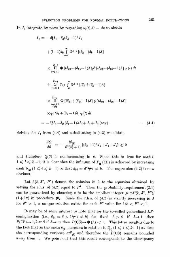
In I1 integrate by parts by regarding icp(?) dt = dv to obtain

/, =

-sii1-st(st-i)?a2

+(i-i)?t ; *'-a[??*+(**-i)A] -co

X f1 (D [??w+(?M-l)AV [??w+(*?-l)A] 9 (?) dt i=1+1

?=I+1 -oo

X n1 <D[?^+(4?-l)Alcp[?^+(4?-l)A]

X9 p**+(**--l)A]<p(*)*

Solving for Z\ from (4.4) and substituting in (4.3) we obtain

and therefore Q(8) is nonincreasing in 8. Since this is true for each /, 1 < / ̂ k?\, it is clear that the infimum of P- (CS) is achieved by increasing

each 8[{] (1 < i ̂ ??1) so that 8^ = ?*V"? 7^ & The expression (4.2) is now

obvious.

Let X(k, 8*, P*) denote the solution in ? to the equation obtained by

setting the r.h.s. of (4.2) equal to P*. Then the probability requirement (2.1) can be guaranteed by choosing n to be the smallest integer > ocA2(k, 8*, P*)/

(l-f2a) in procedure pj. Since the r.h.s. of (4.2) is strictly increasing in ?

for 8* > 1, a unique solution exists for each P*-value for Ijk < P* < 1.

It may be of some interest to note that for the so-called generalized LF

configuration (i.e., 8ki = 8 > 1-y i ?=" k) for fixed ? > 0 if #?> 1 then

P(CS)-> I Ik and if ?-> oo then P(CS)-> O (A) < 1. This latter result is due to

the fact that as the mean 8^

increases in relation to 0[?, (1 ^ i ^ k ?

1) so does

the corresponding variance oc82[k]

and therefore the P(CS) remains bounded

away from 1. We point out that this result corresponds to the discrepancy

352 AJIT C. TAMHANE

between the large sample and the small sample results for the procedures

based on Tmmss that we discussed in Section 3; see Section 4.2.1 for additional

details.

It may also be noted that for fixed k9 8* and P*, the sample size n required to guarantee (2.1) increases with a. As a?? oo, the required sample size n

tends to the smallest integer > A2(&, 8*, P*)/2.

4.1.2. Tables for implementing *Pi- The tables of A(k, 8*, P*) for

k = 2(1)10, 8* =

1.2(0.2)3.0 and P* == 0.99, 0.975, 0.95, 0.90 and 0.75 are

given at the end of the paper.

It may be noted tha+ the r.h.s. of (4.2) equals

where the _$ are standard normal random variables with corr (Z%, Zj) =

p ?

i*2^_+1) (l ^ ?, ?<?, i^zj). The equicoordinate upper 100(1-P*)

percentage points of this multivariate normal distribution have been tabulated

by Gupta, Nagel and Panchapakesan (1973) (they denote the percentage

point by H) for k = 2(1)11(2)51, P* = 0.99, 0.975, 0.95, 0.90, 0.75 and for

selected values of p. Therefore for certain 8*- and ?-values not tabulated by

us, one can use their tables as follows : First compute p =

8*2l(8*2-\-l) and

by referring to the appropriate table read the H -value (note that their N equals our jfc?1). Then A(k, 8*, P*)

= _(?*2+l)*/(?*?1). In fact our A-entries for

8* = 2.0 and 3.0 have been obtained from their tables in the above manner.

The remaining entries were computed on Northwestern University's CDC

6400 computer by solving the integral equation obtained by setting the r.h.s.

of (4.2) equal to P* using the IMSL subroutine ZSYSTM; the integral was

evaluated using the Romberg method of numerical integration. The accuracy

of the calculations was checked by computing some selected entries for 8* = 2.0

and 8* = 3.0 and comparing them with the corresponding entries in the Gupta

et al. tables. The entries given in our tables are rounded off in the fourth

decimal place and should not be off by more than one digit in the last decimal

place reported. We remark that, with the help of interpolation, the tables

in Milton (1963) can also be used to find the ^-values for certain 8*-, k-, and

P*- values.

We finally note that for P*-values close to 1, an excellent approximation

to the sample size can be obtained by using the result that as P* ?> 1

l-P* _ 1 ( ^ ) (^+1 ) exp [-(? _l)W/(a*i+l)]

SELECTION PROBLEMS FOR NORMAL POPULATIONS 353

where ? = ?(Jk, S*, P*) and hence

A^?l+il.og.^). ... (4.5)

(8* -l)2

The proof of (4.5) follows along similar lines as that of Lemma 6.2.1 of Bechhofer, Kiefer and Sobel (1968) and is hence omitted.

4.1.3. Adequacy of the large sample approximation. In this section we

address the problem of how large should n be or e qui valen tly how close should

P* be to 1 in order that the asymptotic approximation (4.1) for PLF (CS) is

valid. To this end we carried out a simulation study for procedure 7?i

employing the estimator of our choice Tmmss f?r k ? 3, 8* = 1.2, a ? 0.5 and

P* = 0.75, 0.90, 0.95, 0.975, 0.99. (A parallel study was carried out for &

employing the estimator T%MMS but the results were quite similar and hence

are not reported here.)

The details of the simulation study are as follows. For each P*, 1000

experiments were run. In each experiment k = 3 independent pairs of r.v.'s

Xi ~ N(8i, a 8\\ri) and ?? ~ a 0f X2(n-xyl(n~ *) wnere generated (by applying the standard transformations to uniform [0, 1] r.v.'s generated by the fortran

library function BANF) where 8X =

82 = 1 and 83

? #*; n was taken to be

the integer closest to oc?.2(k, 8*, P*)/(l + 2a). The value of the estimator

Tmmss was then computed for each 77* from Xt and S2 (1 < i <; 3) using the

formula given in Section 3. Then by applying $>i it was determined wrhether

7T3 (the best population) is correctly selected or not. The estimate of PLF (CS) is given by the fraction of the experiments in which a correct selection is made.

The results of the simulation study are given in Table 4.1 below.

TABLE 4.1. ESTIMATES OF PLf{CS) FOR 7?i EMPLOYING

Tmmss (& = 3, S* = 1.2, a = 0.5, no. of expts.

= 1000)

95% confidence P* n Plf(CS) limits for

Plf(CS)

0.75 15 0.730 (0.7025,0.7575)

0.90 37 0.894 (0.8749,0.9131)

0.95 55 0.939 (0.9242,0.9538)

0.975 74 0.971 (0.9606,0.9814)

0.99 99 0.988 (0.9813,0.9947)

354 AJIT C. TAMHANE!

A study of this table indicates that in all the cases the actual Plf(CS) is not significantly different at 5% level from the specified P*. Thus even for

P* as low as 0.75 the asymptotic approximation is quite good. However the

approximation appears to be consistently deficient (estimated Plf(CS) is less

than the specified P*) although the extent of deficiency is rather small.

Furthermore the deficiency appears to lessen as P* increases.

4.2. Procedure for Goal II (subset selection approach). We propose

the following single-stage procedure iPn for Goal II : Take n ^ 2 inde

pendent observations from each ni9 compute a B.A.N. estimator T? of

di(l < i < k) having the property of being a.s. nonnegative (T?MMS and

Tmmss are two such estimators) and choose the subset of populations using the

following rule : Include ni in the subset <*?)> T% ̂ c_1 Tmax (1 < i < &) where

c (1 < c < oo) is to be chosen so that (2.2) is guaranteed. It should be evident

to the reader that if the T% are not restricted to being a.s. nonnegative then

the selected subset could be empty using the above rule.

4.2.1. Probability of correct selection of jon and its infimum. To find

the minimum value of c necessary to guarantee (2.2) using 70u we first derive

the asymptotic expression for Pe(CS) of pn and then find ite infimum over

??. This is done in the following theorem.

Theorem 4.2 : For ^>u we have that for any 8 e Q

P*(CS)<^ J U <!>[t8kic+(8kic-l)A]9(t)dt, ... (4.6) ? 00 ?=1

where A = {w(l + 2a)/a}*. The infimum of Pq(CS) over ? is achieved for any

8 such that 8k( = 1-y i ̂ k (known as the equal means or E M-configuration)

and

inf Pq(CS) _* J **-i[fc4-(c-l)A] 9 (t) dt. ... (4.7) Q -co

Proof : The proof is exactly analogous to that of Theorem 4.1 and is

hence omitted.

Let c ? c(k9 A, P*) denote the solution in c to the equation obtained

by setting the r.h.s. of (4.7) equal to P*. Then the probability requirement

(2.2) can be guaranteed by using that solution in procedure 7?u. For fixed

A > 0, the r.h.s of (4.7) is strictly increasing in c for c > 1. As c?> 1, the

r.h.s. ?> \?k and as c ?> 00, the r.h.s. ->0(A). Therefore a unique solution in

c exists for each P*-value, \jk < P* < 0(A). This implies the nonexistence

SELECTION PROBLEMS FOR NORMAL POPULATIONS 355

of yjn for P* ;> O(?) which we had earlier pointed out in Section 3. We

might note however that, for all practical purposes, if n ;> (3.5)2/2 > (3.5)2a/

(3+2a) then this upper bound is extremely close to 1. Therefore, pu can

be used to guarantee (2.2) for P*-values usually encountered in practice.

4.2.2. Tables for implementing J0n. To obtain the values of c, the tables

of ? prepared for Goal I can be used in an approximate fashion as follows :

First compute the value of ? = {w(l + 2a)/a}*. In the table for the given value

of k, enter the row corresponding to the specified value of P* and go down the

row until two adjacent ?-entries are found which straddle the computed value

of ?. Read off the corresponding adjacent #*-values. Now note that 8*

plays the role of c and therefore the appropriate value of c can be found by

interpolation between the adjacent 8*-values.

It might be useful to prepare separate tables for the values of

c ? c(k, ?, P*) but we have not attempted to do so in the present paper.

4.2.3. Some properties of "fin : (a) Expected size of the selected subset.

A measure of performance of ?pH is the associated expected size of the subset

say. Eq(S). We have the following asymptotic expression

Eq(S)^ S f n ^[t8ijc+(8ijc-l)?](?(t)dt. ... (4.8) i=i -oo j>;=i

It is often of interest to identify the parameter configuration where the

supremum of (4.8) occurs. For k ? 2, denoting 82X

= 8 it is easy to see that

(4.8) becomes

Ee(S)~<!> \ ift-1)*] +0 l^Z^K) (4 9) 0[ j L (S2c2+l)*J +^ I (c2+82f J

- [ ' ]

The supremum of (4.9) occurs at 8 = 1, i.e., the i?Jf-configuration, and this

supremum equals 2P*. For k > 2 it appears difficult to obtain such a result

because of the lack of the MLR property of N(8, ad2) distribution. We can

only state that sup Eq(S) > EEM(S) = kP*.

Q

(b) Monotonicity property of pu. If pi denotes the probability that t?i

is included in the subset using Pu(l ^ i < k) then we can show using the

method of the proof of Theorem 4.1 that

8i^8j=$pi^pj. ... (4.10)

b4-7

356 ? Jit c. taMhan?

5- Concluding remarks

In this paper we have provided new ranking and selection procedures for the normal means problem when the coefficient of variation is the same

for all populations and is known. When such a situation obtains in practice and suppose, e.g., that the experimenter is interested in Goal I, then our

procedure pj should be used instead of the two-stage procedure of Dudewicz

and Dalai for unknown and unequal variances. We should, however, point out that any comparison between their procedure and our procedure is

precluded because different distance functions are used in the two

procedures.

For future research, it would be useful to extend these procedures to the

case where the common coefficient of variation is unknown.

Appendix

Small sample results

A.l. Distribution of T?MMS . Consider the set-up of Section 3. We shall

derive the exact small sample results only for _?M3fS ; it appears impossible to

obtain the corresponding results for Tmmss- In the following we shall denote

Tlmms by T f?r convenience.

By a simple conditioning argument on S?6 it is easy to see that the c.d.f.

of T\d is given by

0 for t < 0

Fn(*)=i - rA/ir -,

... (A.l)

? ?

VdT P-*?"^ J hn-i(u)du for t > 0,

where hv(?) denotes the p.d.f of a (xl/v)* r.v.

A.2. Procedure for Goal I (indifference-zone approach). In the following theorem we derive an exact expression for Pe(CS) of procedure Pj described

in Section 4.1 and find its infimum over Q(#*).

Theorem A.l : For "pj we have that for any 8 e?i,

Pe(CS) = i- [J\,(0)]*+ S [^?(O)]*-1- i'i K

seS

xj n[Fn(t?u)-Fn(0)]dFM ... (A.2) 0+ i 8

SELECTION PROBLEMS FOR NORMAL POPULATIONS 357

where S = collection of all subsets from {1, 2, ..., k? 1} ?md \s\ =

cardinality

of the set s. The infimum of Pq(CS) over 0,(8*) is achieved at any 8 such that

$ki = <$* for ^f- i ^zk (LF-configuration) and

infPe(GS) = -1f[Fn(0)]k+f[Fn(td*)f-hlFJt).

... (A.3)

Proof ; We have that

Pe(CS) = * Pe{T(i)

= o v ? =? ?}+ 2 Pe {T(iJt) > T(i) Y i ̂ *, K

seS

T(i) >0 Vies, T{i) -OYi^}

= 4[^n(o).i*+ s [p,(o)ri-i^i

which yields (A.2). The proof of the LF-configuration is obvious from

the monotonicity in 8ki of (A.2). The expression (A.3) then follows

immediately.

The probability requirement (2.1) can now be guaranteed by finding the

smallest n which would make the r.h.s. of (A.3) J> P* and using this n in px.

It can be checked that as n-> the r.h.s. of (A.3) ?> 1. However it is not

clear whether it is monotonie in n or not. In view of the computational and

other difficulties cited in Section 2 we have not attempted tabulation of the

exact w-values for selected values of a, k, 8*, P*.

It may be noted that for the generalized LF-configuration (i.e.,

Ski = 8 > 1 Y i =? k) for fixed n > 2, if i-> 1 then Pe(CS)-? \?k and if 8-? oo

then Pe(CS)-> l-Fn(0)-[Fn(0)flk< 1. These results correspond to the

similar ones obtained in the case of large samples.

A.3. Procedure for Goal II (subset selection approach). In the following

theorem, we derive an exact expression for Pe(CS) of pn described in Section

4.2 and find its infimum over ?}.

Theorem A. 2 : For PTi we have that for any 8e?

PB(CS)=-.[Fn(0)Y+ S [?'?(O)]*-1-'?'

seS

x f n [Fn(thiO)-Fr>mdFn(t). ... (A.4)

0+ t 9

358 ajit c. tamhane

The infimum of Pe(CS)

over ?2 is achieved at any 8 such that

?jci = 1 "V* i ̂ k (EM-configuration) and

mf Pe(CS)

= [Pn(0)]* + J [Fn(tc)}k-MFnU).

... (A.5) o w o+

Proof : The proof is similar to that of Theorem A.l and is hence omitted.

Let c ? c(n9 oc9 k9 P*) denote the solution in c to the equation obtained

by setting the r.h.s. of (A.5) equal to P*. Then the probability requirement

(2.2) can be guaranteed by using that value of c in procedure "Pu. The r.h.s.

of (A.5) is strictly increasing in c for c > 1. As c -> 1, the r.h.s.-> \\k and as

c -* oo, the r.h.s.~> [Pn(0)p + 1?P?(0) < 1. Therefore a unique solution in

c exists for each P*9 1/k < P* < [Fn(0)f+1-Fn(0). This implies that 7>n

does not exist for P* > [Fn(0)]k + ] ? Fn(Q) which corresponds to the similar

result obtained in the case of large samples.

We omit the details concerning the exact small sample properties of 7?u

for the sake of brevity.

TABLES. VALUES OF \{k, S*, P*) FOR k = 2(1) 10, d* =

1.2(0.2) 3.0, AND

P* = 0.99, 0.975, 0.95, 0.90, 0.75

k = 2

\ d* \ 1.2 1.4 1.6 1.8 2.0 2.2 2.4 2.6 2.8 3.0

P* \

0.99 18.1667 10.1947 7.5127 5.9869 5.2018 4.6842 4.3197 4.0497 3.8421 3.6782

0.975 15.3081 8.5905 6.3306 5.0449 3.8416 3.9471 3.6400 3.4125 3.2375 3.0990

0.95 12.8479 7.2099 5.3132 4.2341 3.6781 3.3128 3.0550 2.8640 2.7172 2.6008

0.90 10.0127 5.6189 4.1407 3.2997 2.8666 2.5817 2.3808 2.2320 2.1176 2.0264

0.75 5.2641 2.9541 2.1769 1.7348 1.5082 1.3573 1.2517 1.1735 1.1133 1.0665

k = 3

0.99 19.9068 10.9203 7.9521 6.4830 5.6105 5.0340 4.6267 4.3238 4.0900 3.9045

0.975 17.1843 9.4100 6.8410 5.5689 4.8129 4.3138 3.9603 3.6972 3.4944 3.3332

0.95 14.8514 8.1145 5.8871 4.7837 4.1278 3.6944 3.3873 3.1589 2.9824 2.8423

0.90 12.1710 6.6245 4.7897 3.8799 3.3387 2.9808 2.7271 2.5383 2.3923 2.2764

0.75 7.7136 4.1434 2.9601 2.3723 2.0219 1.7897 1.6249 1.5020 1.4068 1.3310

SELECTION PROBLEMS FOR NORMAL POPULATIONS 359

fc = 4

\ 1.2 1.4 1.6 1.8 2.0 2.2 2.4 2.6 2.8 3.0

P*\ 0.99 20.8557 11.4169 8.2958 6.7490 5.8290 5.2206 4.7890 4.4682 4.4202 4.0230

0.975 18.1978 9.9364 7.2031 5.8476 5.0408 4.5072 4.1287 3.8467 3.6285 3.4553

0.95 15.9222 8.6675 6.2657 5.0736 4.3639 3.8942 3.5608 3.3124 3.1202 2.9673

0.90 13.3117 7.2091 5.1873 4.1831 3.5846 3.1881 2.9066 2.6966 2.5342 2.4048

0.75 8.9757 4.7827 2.3909 2.6982 2.2846 2.0099 1.8146 1.6685 1.5549 1.4654

k = 5

0.99 21.5012 11.7535 8.5280 6.9281 5.9757 5.3453 4.8981 4.5644 4.3068 4.1019

0.975 18.8828 10.2911 7.4463 6.0343 5.1930 4.6361 4.2407 3.9459 3.7178 3.5362

0.95 16.6425 9.0380 6.5185 5.2668 4.5211 4.0268 3.6758 3.4140 3.2113 3.0499

0.90 14.0730 7.5982 5.4513 4.3841 3.7474 3.3251 3.0250 2.8010 2.6275 2.4893

0.75 9.8080 5.2036 3.6741 2.9122 2.4568 2.1542 1.9388 1.7777 1.6529 1.5532

k = 6

0.99 21.9843 12.0061 8.7019 7.0619 6.0850 5.4380 4.9788 4.6358 4.3711 4.1600

0.975 19.3960 10.5561 7.6277 6.1733 5.3062 4.7318 4.3238 4.0193 3.7837 3.5960

0.95 17.1799 9.3139 6.7064 5.4105 4.6376 4.1250 3.7608 3.4890 3.2785 3.1107

0.90 14.6384 7.8867 5.6469 4.5327 3.8675 3.4262 3.1124 2.8779 2.6963 2.5515

0.75 10.4214 5.5135 3.8824 3.0695 2.5833 2.2601 2.0300 1.8578 1.7242 1.6175

k :

0.99 22.3735 12.2072 8.8400 7.1681 6.1715 5.5115 5.0427 4.6929 4.4218 4.2065

0.975 19.8041 10.7665 7.7715 6.2832 5.3956 4.8073 4.3893 4.0772 3.8356 3.6429

0.95 17.6060 9.5320 6.8550 5.5238 4.7293 4.2023 3.8278 3.5481 3.3313 3.1586

0.90 15.0854 8.1145 5.8010 4.6497 3.9621 3.5057 3.1810 2.9383 2.7503 2.6003

0.75 10.9035 5.7569 4.0459 3.1928 2.6824 2.3431 2.1014 1.9205 1.7800 1.6679

k = 8

0.99 22.6955 12.3737 8.9543 7.2557 6.2386 5.5720 5.0952 4.7394 4.4634 4 2444

0.975 20.1414 10.9403 7.8901 6.3739 5.4694 4.8695 4.4431 4.1248 3.8782 3.6817

0.95 17.9573 9.7122 6.9769 5.6166 4.8049 4.2659 3.8827 3.5965 3.3747 3.1979

0.90 15.4531 8.3018 5.9277 4.7458 4.0397 3.5709 3.2372 2.9878 2.7945 2.6403

0.75 11.2986 5.9561 4.1797 3.2938 2.7636 2.4110 2.1597 1.9717 1.8257 1.7092

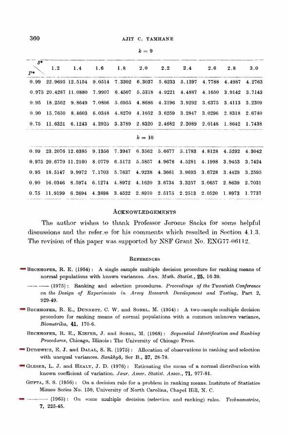
360 A JIT C. TAMHANE

h = 9

^_ _ -

\ 1.2 1.4 1.6 1.8 2.0 2.2 2.4 2.6 2.8 3.0 P* \ _ _

0.99 22.9695 12.5154 9.0514 7.3302 6.3037 5.6233 5.1397 4.7788 4.4987 4.2763

0.975 20.4287 11.0880 7.9907 6.4507 5.5318 4.9221 4.4887 4.1650 3.9142 3.7143

0.95 18.2562 9.8649 7.0806 5.6955 4.8686 4.3196 3.9292 3.6375 3.4113 3.2309

0.90 15.7650 8.4603 6.0348 4.8270 4.1052 3.6259 3.2847 3.0296 2.8318 2.6740

0.75 11.6321 6.1243 4.2925 3.3789 2.8320 2.4682 2.2089 2.0148 1.8642 1.7438

k = 10

0.99 23.2076 12.6385 9.1356 7.3947 6.3562 5.6677 5.1783 4.8128 4.5292 4.3042

0.975 20.6779 11.2160 8.0779 6.5172 5.5857 4.9676 4.5281 4.1998 3.9453 3.7424

0.95 18.5147 9.9972 7.1703 5.7637 4.9238 4.3661 3.9693 3.6728 3.4429 3.2595

0.90 16.0346 8.5974 6.1274 4.8972 4.1620 3.6734 3.3257 3.0657 2.8639 2.7031

0.75 11.9199 6.2694 4.3898 3.4522 2.8910 2.5175 2.2513 2.0520 1.8973 1.7737

ACKNO WLED GEME NTS

The author wishes to thank Professor Jerome Sacks for some helpful discussions and the referee for his comments which resulted in Section 4.1.3.

The revision of this paper was supported by NSF Grant No. ENG77-06112.

References

Bechhofer, R. E. (1954) : A single sample multiple decision procedure for ranking means of

normal populations with known variances, Ann. Math. Statist., 25, 16-39.

?-(1975) : Ranking and selection procedures. Proceedings of the Twentieth Conference on the Design of Experiments in Army Research Development and Testing, Part 2,

929-49.

Bechhofer, R. E., Dunnett, C. W. and Sobel, M. (1954) : A two-sample multiple decision

procedure for ranking means of normal populations with a common unknown variance,

Biometrika, 41, 170-6.

Bechhofer, R. E., Kiefer, J. and Sobel, M. (1968) : Sequential Identification and Ranking

Procedures, Chicago, Illinois : The University of Chicago Press.

Dudewicz, E. J. and Dalal, S. R. (1975) : Allocation of observations in ranking and selection

with unequal variances. Sankhy?, Ser B., 37, 28-78.

Gleser, L. J. and Healy, J. D. (1976) : Estimating the mean of a normal distribution with

known coefficient of variation. Jour. Amer. Statist. Assoc, 71, 977-81.

Gupta, S. S. (1956) : On a decision rule for a problem in ranking means. Institute of Statistics

Mimeo Series No. 150, University of North Carolina, Chapel Hill, N. C.

-(1965) : On some multiple decision (selection and ranking) rules. Technometrics,

7, 225-45.

SELECTION PROBLEMS FOR NORMAL POPULATIONS 361

Gupta, S. S. and Sobel, M. (1957) : On a statistic which arises in selction and ranking prob

lems. -Ann. Math. Statist., 28, 957-67.

Gupta, S. S., Nagel, K. and Panchapakesan, S. (1973) : On the order statistics from equally

correlated normal random variables. Biometrika, 60, 403-13.

Khan, R. A. (1968) : A note on estimating the mean of a normal distribution with known

coefficient of variation. Jour. Amer. Statist., Assoc. 63, 1039-41.

Milton, R. C. (1963) : Tables of the equally correlated multivariate normal probability inte

gral. Tech. Rep. No. 27, Department of Statitics, University of Minnesota, Minneapolis, MN.

Wetherill, G. B. and Ofosu, J. B. (1974) : Selection of the best of k normal populations,

J. Roy. Statist. Soc. Series C, 23, 253-77.

Paper received : July, 1977.

Revised : June, 1978.