Particle Swarm Optimization for HW/SW Partitioningcdn.intechopen.com/pdfs/6253.pdf · 2018-09-25 · Particle Swarm Optimization for HW/SW Partitioning 51 the problem. One of the

3

Particle Swarm Optimization for HW/SW Partitioning

M. B. Abdelhalim and S. E. –D. Habib Electronics and Communications Department, Faculty of Engineering - Cairo University

Egypt

1. Introduction

Embedded systems typically consist of application specific hardware parts and programmable parts, e.g. processors like DSPs, core processors or ASIPs. In comparison to the hardware parts, the software parts are much easier to develop and modify. Thus, software is less expensive in terms of costs and development time. Hardware, however, provides better performance. For this reason, a system designer's goal is to design a system fulfilling all system constraints. The co-design phase, during which the system specification is partitioned onto hardware and programmable parts of the target architecture, is called Hardware/Software partitioning. This phase represents one key issue during the design process of heterogeneous systems. Some early co-design approaches [Marrec et al. 1998, Cloute et al. 1999] carried out the HW/SW partitioning task manually. This manual approach is limited to small design problems with small number of constituent modules. Additionally, automatic Hardware/Software partitioning is of large interest because the problem itself is a very complex optimization problem. Varieties of Hardware/Software partitioning approaches are available in the literature. Following Nieman [1998], these approaches can be distinguished by the following aspects: 1. The complexity of the supported partitioning problem, e.g. whether the target

architecture is fixed or optimized during partitioning. 2. The supported target architecture, e.g. single-processor or multi-processor, ASIC or

FPGA-based hardware. 3. The application domain, e.g. either data-flow or control-flow dominated systems. 4. The optimization goal determined by the chosen cost function, e.g. hardware

minimization under timing (performance) constraints, performance maximization under resource constraints, or low power solutions.

5. The optimization technique, including heuristic, probabilistic or exact methods, compared by computation time and the quality of results.

6. The optimization aspects, e.g. whether communication and/or hardware sharing are taken into account.

7. The granularity of the pieces for which costs are estimated for partitioning, e.g. granules at the statement, basic block, function, process or task level.

8. The estimation method itself, whether the estimations are computed by special estimation tools or by analyzing the results of synthesis tools and compilers.

www.intechopen.com

Particle Swarm Optimization

50

9. The cost metrics used during partitioning, including cost metrics for hardware implementations (e.g. execution time, chip area, pin requirements, power consumption, testability metrics), software cost metrics (e.g. execution time, power consumption, program and data memory usage) and interface metrics (e.g. communication time or additional resource-power costs).

10. The number of these cost metrics, e.g. whether only one hardware solution is considered for each granule or a complete Area/Time curve.

11. The degree of automation. 12. The degree of user-interaction to exploit the valuable experience of the designer. 13. The ability for Design-Space-Exploration (DSE) enabling the designer to compare

different partitions and to find alternative solutions for different objective functions in short computation time.

In this Chapter, we investigate the application of the Particle Swarm Optimization (PSO) technique for solving the Hardware/Software partitioning problem. The PSO is attractive for the Hardware/Software partitioning problem as it offers reasonable coverage of the design space together with O(n) main loop's execution time, where n is the number of proposed solutions that will evolve to provide the final solution. This Chapter is an extended version of the authors’ 2006 paper [Abdelhalim et al. 2006]. The organization of this chapter is as follows: In Section 2, we introduce the HW/SW partitioning problem. Section 3 introduces the Particle Swarm Optimization formulation for HW/SW Partitioning problem followed by a case study. Section 4 introduces the technique extensions, namely, hardware implementation alternatives, HW/SW communications modeling, and fine tuning algorithm. Finally, Section 5 gives the conclusions of our work.

2. HW/SW Partitioning

The most important challenge in the embedded system design is partitioning; i.e. deciding which components (or operations) of the system should be implemented in hardware and which ones in software. The granularity of each component can be a single instruction, a short sequence of instructions, a basic block or a function (procedure). To clarify the HW/SW partitioning problem, let us represent the system by a Data Flow Graph (DFG) that defines the sequencing of the operations starting from the input capture to the output evaluation. Each node in this DFG represents a component (or operation). Implementing a given component in HW or in SW implies different delay/ area/ power/ design-time/ time-to-market/ … design costs. The HW/SW partitioning problem is, thus, an optimization problem where we seek to find the partition ( an assignment vector of each component to HW or SW) that minimizes a user-defined global cost function (or functions) subject to given area/ power/ delay …constraints. Finding an optimal HW/SW partition is hard because of the large number of possible solutions for a given granularity of the “components” and the many different alternatives for these granularities. In other words, the HW/SW partitioning problem is hard since the design (search) space is typically huge. The following survey overviews the main algorithms used to solve the HW/SW partitioning problem. However, this survey is by no means comprehensive. Traditionally, partitioning was carried out manually as in the work of Marrec et al. [1998] and Cloute et al. [1999]. However, because of the increase of complexity of the systems, many research efforts aimed at automating the partitioning as much as possible. The suggested partition approaches differ significantly according to the definition they used to

www.intechopen.com


51

the problem. One of the main differences is whether to include other tasks (such as scheduling where starting times of the components should be determined) as in Lopez-Vallejo et al [2003] and in Mie et al. [2000], or just map components to hardware or software only as in the work of Vahid [2002] and Madsen et al [1997]. Some formulations assign communication events to links between hardware and/or software units as in Jha and Dick [1998]. The system to be partitioned is generally given in the form of task graph, the graph nodes are determined by the model granularity, i.e. the semantic of a node. The node could represent a single instruction, short sequence of instructions [Stitt et al. 2005], basic block [Knudsen et al. 1996], a function or procedure [Ditzel 2004, and Armstrong et al. 2002]. A flexible granularity may also be used where a node can represent any of the above [Vahid 2002; Henkel and Ernst 2001]. Regarding the suggested algorithms, one can differentiate between exact and heuristic methods. The proposed exact algorithms include, but are not limited to, branch-and-bound [Binh et al 1996], dynamic programming [Madsen et al. 1997], and integer linear programming [Nieman 1998; Ditzel 2004]. Due to the slow performance of the exact algorithms, heuristic-based algorithms are proposed. In particular, Genetic algorithms are widely used [Nieman 1998; Mann 2004] as well as simulated annealing [Armstrong et al 2002; Eles et al. 1997], hierarchical clustering [Eles et al. 1997], and Kernighan-Lin based algorithms such as in [Mann 2004]. Less popular heuristics are used such as Tabu search [Eles et al. 1997] and greedy algorithms [Chatha and Vemuri 2001]. Some researchers used custom heuristics, such as Maximum Flow-Minimum Communications (MFMC) [Mann 2004], Global Criticality/Local Phase (GCLP) [Kalavade and Lee 1994], process complexity [Adhipathi 2004], the expert system presented in [Lopez-Vallejo et al. 2003], and Balanced/Unbalanced partitioning (BUB) [Stitt 2008]. The ideal Hardware/Software partitioning tool produces automatically a set of high-quality partitions in a short, predictable computation time. Such tool would also allow the designer to interact with the partitioning algorithm. De Souza et al. [2003] propose the concepts of ”quality requisites” and a method based on Quality Function Deployment (QFD) as references to represent both the advantages and disadvantages of existing HW/SW partitioning methods, as well as, to define a set of features for an optimized partitioning algorithm. They classified the algorithms according to the following criterion: 1. Application domain: whether they are "multi-domain" (conceived for more than one or

any application domain, thus not considering particularities of these domains and being technology-independent) or "specific domain" approaches.

2. The target architecture type. 3. Consideration for the HW-SW communication costs. 4. Possibility of choosing the best implementation alternative of HW nodes. 5. Possibility of sharing HW resources among two or more nodes. 6. Exploitation of HW-SW parallelism. 7. Single-mode or multi-mode systems with respect to the clock domains. In this Chapter, we present the use of the Particle Swarm Optimization techniques to solve the HW/SW partitioning problem. The aforementioned criterions will be implicitly considered along the algorithm presentation.

3. Particle swarm optimization

Particle swarm optimization (PSO) is a population based stochastic optimization technique developed by Eberhart and Kennedy in 1995 [Kennedy and Eberhart 1995; Eberhart and

www.intechopen.com


52

Kennedy 1995; Eberhart and Shi 2001]. The PSO algorithm is inspired by social behavior of bird flocking, animal hording, or fish schooling. In PSO, the potential solutions, called particles, fly through the problem space by following the current optimum particles. PSO has been successfully applied in many areas. A good bibliography of PSO applications could be found in the work done by Poli [2007].

3.1 PSO algorithm

As stated before, PSO simulates the behavior of bird flocking. Suppose the following scenario: a group of birds is randomly searching for food in an area. There is only one piece of food in the area being searched. Not all the birds know where the food is. However, during every iteration, they learn via their inter-communications, how far the food is. Therefore, the best strategy to find the food is to follow the bird that is nearest to the food. PSO learned from this bird-flocking scenario, and used it to solve optimization problems. In PSO, each single solution is a "bird" in the search space. We call it "particle". All of particles have fitness values which are evaluated by the fitness function (the cost function to be optimized), and have velocities which direct the flying of the particles. The particles fly through the problem space by following the current optimum particles. PSO is initialized with a group of random particles (solutions) and then searches for optima by updating generations. During every iteration, each particle is updated by following two "best" values. The first one is the position vector of the best solution (fitness) this particle has achieved so far. The fitness value is also stored. This position is called pbest. Another "best" position that is tracked by the particle swarm optimizer is the best position, obtained so far, by any particle in the population. This best position is the current global best and is called gbest. After finding the two best values, the particle updates its velocity and position according to equations (1) and (2) respectively.

)xgbest(rc)xpbest(rcwvv i

kk22

i

k

i

11

i

k

i

1k −+−+=+ (1)

i

1k

i

k

i

1k vxx ++ += (2)

where ikv is the velocity of ith particle at the kth iteration, i

kx is current the solution (or

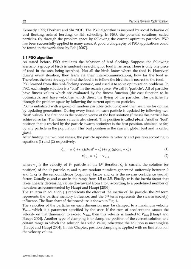
position) of the ith particle. r1 and r2 are random numbers generated uniformly between 0 and 1. c1 is the self-confidence (cognitive) factor and c2 is the swarm confidence (social) factor. Usually c1 and c2 are in the range from 1.5 to 2.5. Finally, w is the inertia factor that takes linearly decreasing values downward from 1 to 0 according to a predefined number of iterations as recommended by Haupt and Haupt [2004]. The 1st term in equation (1) represents the effect of the inertia of the particle, the 2nd term represents the particle memory influence, and the 3rd term represents the swarm (society) influence. The flow chart of the procedure is shown in Fig. 1. The velocities of the particles on each dimension may be clamped to a maximum velocity Vmax, which is a parameter specified by the user. If the sum of accelerations causes the velocity on that dimension to exceed Vmax, then this velocity is limited to Vmax [Haupt and Haupt 2004]. Another type of clamping is to clamp the position of the current solution to a certain range in which the solution has valid value, otherwise the solution is meaningless [Haupt and Haupt 2004]. In this Chapter, position clamping is applied with no limitation on the velocity values.

www.intechopen.com


53

Figure 1. PSO Flow chart

3.2 Comparisons between GA and PSO

The Genetic Algorithm (GA) is an evolutionary optimizer (EO) that takes a sample of possible solutions (individuals) and employs mutation, crossover, and selection as the primary operators for optimization. The details of GA are beyond the scope of this chapter, but interested readers can refer to Haupt and Haupt [2004]. In general, most of evolutionary techniques have the following steps:

1. Random generation of an initial population. 2. Reckoning of a fitness value for each subject. This fitness value depends directly on

the distance to the optimum. 3. Reproduction of the population based on fitness values. 4. If requirements are met, then stop. Otherwise go back to step 2.

From this procedure, we can learn that PSO shares many common points with GA. Both algorithms start with a group of randomly generated population and both algorithms have fitness values to evaluate the population, update the population and search for the optimum with random techniques, and finally, check for the attainment of a valid solution. On the other hand, PSO does not have genetic operators like crossover and mutation. Particles update themselves with the internal velocity. They also have memory, which is important to the algorithm (even if this memory is very simple as it stores only pbesti and gbestk positions).

www.intechopen.com


54

Also, the information sharing mechanism in PSO is significantly different: In GAs, chromosomes share information with each other. So the whole population moves like one group towards an optimal area even if this move is slow. In PSO, only gbest gives out the information to others. It is a one-way information sharing mechanism. The evolution only looks for the best solution. Compared with GA, all the particles tend to converge to the best solution quickly in most cases as shown by Eberhart and Shi [1998] and Hassan et al. [2004]. When comparing the run-time complexity of the two algorithms, we should exclude the similar operations (initialization, fitness evaluation, and termination) form our comparison. We exclude also the number of generations, as it depends on the optimization problem complexity and termination criteria (our experiments in Section 3.4.2 indicate that PSO needs lower number of generations than GA to reach a given solution quality). Therefore, we focus our comparison to the main loop of the two algorithms. We consider the most time-consuming processes (recombination in GA as well as velocity and position update in PSO). For GA, if the new generation replaces the older one, the recombination complexity is O(q), where q is group size for tournament selection. In our case, q equals the Selection rate*n, where n is the size of population. However, if the replacement strategy depends on the fitness of the individual, a sorting process is needed to determine which individuals to be replaced by which new individuals. This sorting is important to guarantee the solution quality. Another sorting process is needed any way to update the rank of the individuals at the end of each generation. Note that the quick sorting complexity ranges from O(n2) to O(nlog

2 n) [Jensen 2003, Harris and Ross 2006].

In the other hand, for PSO, the velocity and position update processes complexity is O(n) as there is no need for pre-sorting. The algorithm operates according to equations (1) and (2) on each individual (particle) [Rodriguez et al. 2008]. From the above discussion, GA's complexity is larger than that of PSO. Therefore, PSO is simpler and faster than GA.

3.3 Algorithm Implementation

The PSO algorithm is written in the MATLAB program environment. The input to the program is a design that consists of the number of nodes. Each node is associated with cost parameters. For experimental purpose, these parameters are randomly generated. The used cost parameters are: A Hardware implementation cost: which is the cost of implementing that node in hardware (e.g. number of gates, area, or number of logic elements). This hardware cost is uniformly and randomly generated in the range from 1 to 99 [Mann 2004]. A Software implementation cost: which is the cost of implementing that node in software (e.g. execution delay or number of clock cycles). This software cost is uniformly and randomly generated in the range from 1 to 99 [Mann 2004]. A Power implementation cost: which is the power consumption if the node is implemented in hardware or software. This power cost is uniformly and randomly generated in the range from 1 to 9. We use a different range for Power consumption values to test the addition of other cost terms with different range characteristics. Consider a design consisting of m nodes. A possible solution (particle) is a vector of m elements, where each element is associated to a given node. The elements assume a “0” value (if node is implemented in software) or a “1” value (if the node is implemented in hardware). There are n initial particles; the particles (solutions) are initialized randomly.

www.intechopen.com


55

The velocity of each node is initialized in the range from (-1) to (1), where negative velocity means moving the particle toward 0 and positive velocity means moving the particle toward 1. For the main loop, equations (1), (2) are evaluated in each loop. If the particle goes outside the permissible region (position from 0 to 1), it will be kept on the nearest limit by the aforementioned clamping technique. The cost function is called for each particle, the used cost function is a normalized weighted sum of the hardware, software, and power cost of each particle according to equation (3).

⎭⎬⎫

⎩⎨⎧

γ+β+α=tcosallPOWER

tcosPOWER

tcosallSW

tcosSW

tcosallHW

tcosHW*100Cost (3)

where allHWcost (allSWcost) is the Maximum Hardware (Software) cost when all nodes are mapped to Hardware (Software), and allPOWERcost is the average of the power cost of

all-Hardware solution and all-Software solution. α, β, and γ are weighting factors. They are set by the user according to his/her critical design parameters. For the rest of this chapter, all the weighting factors are considered equal unless otherwise mentioned. The multiplication by 100 is for readability only. The HWCost (SWCost) term represent the cost of the partition implemented in hardware (software), it could represent the area and the delay of the partition (the area and the delay of the software partition). However, the software cost has a fixed (CPU area) term that is independent on the problem size. The weighted sum of normalized metrics is a classical approach to transform Multi-objective Optimization problems into a single objective optimization [Donoso and Fabregat 2007] The PSO algorithm proceeds according to the flow chart shown in Fig. 1. For simplicity, the cost value could be considered as the inverse of the fitness where good solutions have low cost values. According to equations (1) and (2), the particle nodes values could take any value between 0 and 1. However, as a discrete, i.e. binary, partitioning problem, the nodes values must take values of 1 or 0. Therefore, the position value is rounded to the nearest integer [Hassan et al. 2004]. The main loop is terminated when the improvement in the global best solution gbest for the

last number iterations is less than a predefined value (ε). The number of these iterations and

the value of (ε) are user controlled parameters. For GA parameters, the most important parameters are:

• Selection rate which is the percentage of the population members that are kept unchanged while the others go under the crossover operators.

• Mutation rate which is the percentage of the population that undergo the gene alteration process after each generation.

• The mating technique which determines the mechanism of generating new children form the selected parents.

3.4 Results

3.4.1 Algorithms parameters

The following experiments are performed on a Pentium-4 PC with 3GHz processor speed, 1 GB RAM and WinXP operating system. The experiments were performed using MATLAB 7

www.intechopen.com


56

program. The PSO results are compared with the GA. Common parameters between the two algorithms are as follows:

No. of particles (Population size) n = 60, design size m = 512 nodes, ε = 100 * eps, where eps is defined in MATLAB as a very small (numerical resolution) value and equals 2.2204*10-16 [Hanselman and Littlefield 2001]. For PSO, c1 = c2 = 2, w starts at 1 and decreases linearly until reaching 0 after 100 iterations. Those values are suggested in [Shi and Eberhart 1998; Shi and Eberhart 1999; Zheng et al. 2003]. To get the best results for GA, the parameters values are chosen as suggested in [Mann 2004; Haupt and Haupt 2004] where Selection rate = 0.5, Mutation rate = 0.05 , and The mating is performed using randomly selected single point crossover. The termination criterion is the same for both PSO and GA. The algorithm stops after 50 unchanged iterations, but at least 100 iterations must be performed to avoid quick stagnation.

3.4.2 Algorithm results

Figures 2 and 3 shows the best cost as well as average population cost of GA and PSO respectively.

0 2 0 4 0 6 0 8 0 1 0 0 1 2 01 3 0

1 3 5

1 4 0

1 4 5

1 5 0

1 5 5H W / S W p a rt i t io n in g u s in g G A

G e n e ra t io n

Cost

B e s t

P o p u la t io n A ve ra g e

Figure 2. GA Solution

As shown in the figures, the initialization is the same, but at the end, the best cost of GA is 143.1 while for PSO it is 131.6. This result represents around 8% improvement in the result quality in favor of PSO. Another advantage of PSO is its performance (speed), as it terminates after 0.609 seconds while GA terminates after 0.984 seconds. This result represents around 38% improvement in performance in favor of PSO. The results vary slightly from one run to another due to the random initialization. Hence, decisions based on a single run are doubtful. Therefore, we ran the two algorithms 100 times for the same input and took the average of the final costs. We found the average best cost of GA is 143 and it terminates after 155 seconds, while for the PSO the average best cost was 131.6 and it terminates after 110.6 seconds. Thus, there are 8% improvement in the result quality and 29% speed improvement.

www.intechopen.com


57

0 20 40 60 80 100 120130

135

140

145

150

155

Generation

Cost

HW/SW partitioning using PSO

Best

Population average

Global Best

Figure 3. PSO Solution

3.4.3 Improved Algorithms.

To further enhance the quality of the results, we tried cascading two runs of the same algorithm or of different algorithms. There are four possible cascades of this type: GA followed by another GA run (GA-GA algorithm), GA followed by PSO run (GA – PSO algorithm), PSO followed by GA run (PSO-GA algorithm), and finally PSO followed by another PSO run (PSO-PSO algorithm). For these cascaded algorithms, we kept the parameters values the same as in the Section 3.4.1. Only the last combination, PSO-PSO algorithm proved successful. For GA-GA algorithm, the second GA run is initialized with the final results of the first GA run. This result can be explained as follows. When the population individuals are similar, the crossover operator yields no improvements and the GA technique depends on the mutation process to escape such cases, and hence, it slowly escapes local minimums. Therefore, cascading several GA runs takes a very long time to yield significant improvement in results. The PSO-GA algorithm did not fair any better. This negative result can be explained as follows. At the end of the first PSO run, the whole swarm particles converge around a certain point (solution) as shown in Fig. 3. Thus, the GA is initialized with population members of close fitness with small or no diversity. In fact, this is a poor initialization of the GA, and hence it is not expected to improve the PSO results of the first step of this algorithm significantly. Our numerical results confirmed this conclusion The GA-PSO algorithm was not also successful. Figures 4 and 5 depict typical results for this algorithm. PSO starts with the final solutions of the GA stage (The GA best output cost is ~143, and the population final average is ~147) and continues the optimization until it terminates with a best output cost equals ~132. However, this best output cost value is achieved by PSO alone as shown in Fig. 3. This final result could be explained as the PSO behavior is not strongly dependent on the initial particles position obtained by GA due to the random velocities assigned to the particles at the beginning of PSO phase. Notice that, in Fig. 5, the cost increases at the beginning due to the random velocities that force the particles to move away from the positions obtained by GA phase.

www.intechopen.com


58

0 50 100 150130

132

134

136

138

140

142

144

146

148

150

152HW /S W part it ioning us ing G A

G eneration

Cost

B est

P opula tion A verage

Figure 4. GA output of GA-PSO

0 1 0 2 0 3 0 4 0 5 0 6 0 7 01 3 0

1 3 2

1 3 4

1 3 6

1 3 8

1 4 0

1 4 2

1 4 4

1 4 6

1 4 8

1 5 0

1 5 2

G e n e r a t i o n

Cost

H W / S W p a r t i t i o n in g u s in g P S

B e s t

P o p u la t i o n A v e r a g e

G lo b a l B e s t

Figure 5. PSO output of GA-PSO

3.4.4 Re-exited PSO algorithm.

As the PSO proceeds, the effect of the inertia factor (w) is decreased until reaching 0.

Therefore, i

1kv + at the late iterations depends only on the particle memory influence and the

swarm influence (2nd and 3rd terms in equation (1)). Hence, the algorithm may give non-global optimum results. A hill-climbing algorithm is proposed, this algorithm is based on the assumption that if we take the run's final results (particles positions) and start allover again with (w) = 1 and re-initialize the velocity (v) with new random values, and keeping the pbest and gbest vectors in the particles memories, the results can be improved. We found that the result quality is improved with each new round until it settles around a certain value. Fig. 6 plots the best cost in each round. The curve starts with cost ~133 and settles at round number 30 with cost value ~116.5 which is significantly below the results obtained in the previous two subsections (about 15% quality improvement). The program

www.intechopen.com


59

performed 100 rounds, but it could be modified to stop earlier by using a different termination criterion (i.e. if the result remains unchanged for a certain number of rounds).

0 1 0 2 0 3 0 4 0 5 0 6 0 7 0 8 0 9 0 1 0 01 1 6

1 1 8

1 2 0

1 2 2

1 2 4

1 2 6

1 2 8

1 3 0

1 3 2

1 3 4

R o u n d

Best

Cost

H W / S W p a r t i t i o n i n g u s in g r e - e x c i t e d P S O

Figure 6. Successive improvements in Re-excited PSO

As the new algorithm depends on re-exciting new randomized particle velocities at the beginning of each round, while keeping the particle positions obtained so far, it allows another round of domain exploration. We propose to name this successive PSO algorithm as the Re-excited PSO algorithm. In nature, this algorithm looks like giving the birds a big push after they are settled in their best position. This push re-initializes the inertia and speed of the birds so they are able to explore new areas, unexplored before. Hence, if the birds find a better place, they will go there, otherwise they will return back to the place from where they were pushed. The main reason of the advantage of re-excited PSO over successive GA is as follows: The PSO algorithm is able to switch a single node from software to hardware or vice versa during a single iteration. Such single node flipping is difficult in GA as the change is done through crossover or mutation. However, crossover selects large number of nodes in one segment as a unit of operation. Mutation toggles the value of a random number of nodes. In either case, single node switching is difficult and slow. This re-excited PSO algorithm can be viewed as a variant of the re-start strategies for PSO published elsewhere. However, our re-excited PSO algorithm is not identical to any of these previously published re-starting PSO algorithms as discussed below. In Settles and Soule [2003], the restarting is done with the help of Genetic Algorithm operators, the goal is to create two new child particles whose position is between the parents position, but accelerated away from the current direction to increase diversity. The children’s velocity vectors are exchanged at the same node and the previous best vector is set to the new position vector, effectively restarting the children’s memory. Obviously, our restarting strategy is different in that it depends on pure PSO operators. In Tillett et al. [2005], the restarting is done by spawning a new swarm when stagnation occurs, i.e. the swarm spawns a new swarm if a new global best fitness is found. When a swarm spawns a new swarm, the spawning swarm (parent) is unaffected. To form the spawned (child) swarm, half of the children particles are randomly selected from the parent swarm and the other half are randomly selected from a random member of the swarm collection (mate). Swarm creation is suppressed when there are large numbers of swarms in

www.intechopen.com


60

existence. Obviously, our restarting strategy is different in that it depends on a single swarm. In Pasupuleti and Battiti [2006], the Gregarious PSO or G-PSO, the population is attracted by the global best position and each particle is re-initialized with a random velocity if it is stuck close to the global best position. In this manner, the algorithm proceeds by aggressively and greedily scouting the local minima whereas Basic-PSO proceeds by trying to avoid them. Therefore, a re-initialization mechanism is needed to avoid the premature convergence of the swarm. Our algorithm differs than G-PSO in that the re-initialization strategy depends on the global best particle not on the particles that stuck close to the global best position which saves a lot of computations needed to compare each particle position with the global best one. Finally, the re-start method of Van den Bergh [2002], the Multi-Start PSO (MPSO), is the nearest to our approach, except that when the swarm converges to a local optima. The MPSO records the current position and re-initialize the positions of the particles. The velocities are not re-initialized as MPSO depends on a different version of the velocity equation that guarantees that the velocity term will never reach zero. The modified algorithm is called Guaranteed Convergence PSO (GCPSO). Our algorithm differs in that we use the velocity update equation defined in Equation (1) and our algorithm re-initializes the velocity and the inertia of the particles but not the positions at the restart.

3.5 Quality and Speed Comparison between GA, PSO, and re-excited PSO

For the sake of fair comparison, we assumed that we have different designs where their sizes range from 5 nodes to 1020 nodes. We used the same parameters as described in previous experiments and we ran the algorithms on each design size 10 times and took the average results. Another stopping criterion is added to the re-excited PSO where it stops when the best result is the same for the last 10 rounds. Fig. 7 represents the design quality improvement of PSO over GA, re-excited PSO over GA, and re-excited PSO over PSO. We noticed that when the design size is around 512, the improvement is about 8% which confirms the quality improvement results obtained in Section 3.4.2.

0 100 200 300 400 500 600 700 800 900 10000

5

10

15

20

25

30

Qualit

y Im

pro

vem

ent

Design Size in Nodes

PSO over GA

Re-excited PSO over GA

Re-excited PSO over PSO

Figure 7. Quality improvement

www.intechopen.com


61

0 100 200 300 400 500 600 700 800 900 1000-30

-20

-10

0

10

20

30

40

50

60

70

Design Size in Nodes

Speed Im

pro

vem

ent

Figure 8. Speed improvement

Fig. 8 represents the performance (speed) improvement of PSO over GA (original and fitted curve, the curve fitting is done using MATLAB Basic Fitting tool). Re-excited PSO is not included as it depends on multi-round scheme where it starts a new round internally when the previous round terminates, while GA and PSO runs once and produces their outputs when a termination criterion is met. It is noticed that in a few number of points in Fig. 8, the speed improvement is negative which means that GA finishes before PSO, but the design quality in Fig. 7 does not show any negative values. Fig. 7 also shows that, on the average, PSO outperforms GA by a ratio of 7.8% improvements in the result quality and Fig. 8 shows that, on the average, PSO outperforms GA by a ratio 29.3% improvement in speed. On the other hand, re-excited PSO outperforms GA by an average ratio of 17.4% in design quality, and outperforms normal PSO by an average ratio of 10.5% in design quality. Moreover, Fig. 8 could be divided into three regions. The first region is the small size designs region (lower than 400 nodes) where the speed improvement is large (from 40% to 60%). The medium size design region (from 400 to 600 nodes) depicts an almost linear decrease in the speed improvement from 40% to 10%. The large size design region (bigger than 600 nodes) shows an almost constant (around 10%) speed improvement, with some cases where GA is faster than PSO. Note that most of the practical real life HW/SW partitioning problems belong to the first region where the number of nodes < 400.

3.6 Constrained Problem Formulation

3.6.1 Constraints definition and violation handling

In embedded systems, the constraints play an important role in the success of a design, where hard constraints mean higher design effort and therefore a high need for automated tools to guide the designer in critical design decisions. In most of the cases, the constraints are mainly the software deadline times (for real-time systems) and the maximum available area for hardware. For simplicity, we will refer to them as software constraint and hardware constraint respectively. Mann [2004] divided the HW/SW partitioning problem into 5 sub-problems (P1 – P5). The unconstrained problem (P5) is discussed in Section 3.3. The P1 problem involves with both

www.intechopen.com


62

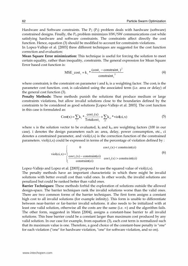
Hardware and Software constraints. The P2 (P3) problem deals with hardware (software) constrained designs. Finally, the P4 problem minimizes HW/SW communications cost while satisfying hardware and software constraints. The constraints affect directly the cost function. Hence, equation (3) should be modified to account for constraints violations. In Lopez-Vallejo et al. [2003] three different techniques are suggested for the cost function correction and evaluation: Mean Square Error minimization: This technique is useful for forcing the solution to meet certain equality, rather than inequality, constraints. The general expression for Mean Square Error based cost function is:

2

i

2

ii

iiconstraint

)constraint(cost*k MSE_cost

−= (4)

where constrainti is the constraint on parameter i and ki is a weighting factor. The costi is the parameter cost function. costi is calculated using the associated term (i.e. area or delay) of the general cost function (3). Penalty Methods: These methods punish the solutions that produce medium or large constraints violations, but allow invalid solutions close to the boundaries defined by the constraints to be considered as good solutions [Lopez-Vallejo et al. 2003]. The cost function in this case is formulated as:

∑ ∑+=i ci

ci

i

ii )x,ci(viol*k

tcosTotal

)x(tcos*k)x(Cost (5)

where x is the solution vector to be evaluated, ki and kci are weighting factors (100 in our case). i denotes the design parameters such as: area, delay, power consumption, etc., ci denotes a constrained parameter, and viol(ci,x) is the correction function of the constrained parameters. viol(ci,x) could be expressed in terms of the percentage of violation defined by :

⎪⎪⎩⎪⎪⎨⎧

>−

<

=

)ciint(constra)x(tcos(ci)constraint

(ci)constraint)x(tcos

)ciint(constra)x(tcos0

x)viol(ci,

ii

i

(6)

Lopez-Vallejo and Lopez et al. [2003] proposed to use the squared value of viol(ci,x). The penalty methods have an important characteristic in which there might be invalid solutions with better overall cost than valid ones. In other words, the invalid solutions are penalized but could be ranked better than valid ones. Barrier Techniques: These methods forbid the exploration of solutions outside the allowed design-space. The barrier techniques rank the invalid solutions worse than the valid ones. There are two common forms of the barrier techniques. The first form assigns a constant high cost to all invalid solutions (for example infinity). This form is unable to differentiate between near-barrier or far-barrier invalid solutions. it also needs to be initialized with at least one valid solution, otherwise all the costs are the same (i.e. ∞) and the algorithm fails. The other form, suggested in Mann [2004], assigns a constant-base barrier to all invalid solutions. This base barrier could be a constant larger than maximum cost produced by any valid solution. In our case for example, from equation (3), each cost term is normalized such that its maximum value is one. Therefore, a good choice of the constant-base penalty is "one" for each violation ("one" for hardware violation, "one" for software violation, and so on).

www.intechopen.com


63

3.6.2 Constraints modeling

In order to determine the best method to be adopted, a comparison between the penalty methods (first order or second order percentage violation term) and the barrier methods (infinity vs. constant-base barrier) is performed. The details of the experiments are not shown here for the sake of brevity. Our experiments showed that combining the constant-base barrier method with any penalty method (first-order error or second-order error term) gives higher quality solutions and guarantees that no invalid solutions beat valid ones. Hence, in the following experiments, equation (7) will be used as the cost function form. Our experiments further indicate that the second-order error penalty method gives a slight improvement over first-order one. For double constraints problem (P1), generating valid initial solutions is hard and time consuming, and hence, the barrier methods should be ruled out for such problems. When dealing with single constraint problems (P2 and P3), one can use the Fast Greedy Algorithm (FGA) proposed by Mann [2004] to generate valid initial solutions. FGA starts by assigning all nodes to the unconstrained side. It then proceeds by randomly moving nodes to the constrained side until the constraint is violated.

))ci(viol_Barrier)x,ci(viol_Penalty(ktcosTotal

)x(tcos*k)x(Cost

i cici

i

ii ++=∑ ∑ (7)

3.6.3 Single constraint experiments

As P2 and P3 are treated the same in our formulation, we consider the software constrained problem (P3) only. Two experiments were performed, the first one with relaxed constraint where the deadline (Maximum delay) is 40% of all-Software solution delay, the second one is a hard real-time system where the deadline is 15% of the all-Software solution delay. The parameters used are the same as in Section 3.4. Fast Greedy Algorithm is used to generate the initial solutions and re-excited PSO is performed for 10 rounds. In the cases of GA and normal PSO only, all results are based on averaging the results of 100 runs. For the first experiment; the average quality of the GA is ~ 137.6 while for PSO it is ~ 131.3, and for re-excited PSO it is ~ 120. All final solutions are valid due to the initialization scheme used (Fast Greedy Algorithm). For the second experiment, the average quality of the solution of GA is ~ 147 while for PSO it is ~ 137 and for re-excited PSO it is ~ 129. The results confirm our earlier conclusion that the re-excited PSO again outperforms normal PSO and GA, and that the normal PSO again outperforms GA.

3.6.4 Double constraints experiments

When testing P1 problems, the same parameters as the single-constrained case are used except that FGA is not used for initialization. Two experiments were performed: balanced constraints where maximum allowable hardware area is 45% of the area of the all-Hardware solution and the maximum allowable software delay is 45% of the delay of the all-Software solution. The other one is an unbalanced-constraints problem where maximum allowable hardware area is 60% of area of the all-Hardware solution and the maximum allowable software delay is 20% of the delay of the all-Software solution. Note that these constraints are used to guarantee that at least a valid solution exists.

www.intechopen.com


64

For the first experiment, the average quality of the solution of GA is ~ 158 and invalid solutions are obtained during the first 22 runs out of xx total runs. The best valid solution cost was 137. For PSO the average quality is ~ 131 with valid solutions during all the runs. The best valid solution cost was 128.6. Finally for the re-excited PSO; the final solution quality is 119.5. It is clear that re-excited PSO again outperforms both PSO and GA. For the second experiment; the average quality of the solution of GA is ~ 287 and no valid solution is obtained during the runs. Note that a constant penalty barrier of value 100 is added to the cost function in the case of a violation. For PSO the average quality is ~ 251 and no valid solution is obtained during the runs. Finally, for the re-excited PSO, the final solution quality is 125 (As valid solution is found in the seventh round). This shows the performance improvement of re-excited PSO over both PSO and GA. Hence, for the rest of this Chapter, we will use the terms PSO and re-excited PSO interchangeably to refer to the re-excited algorithm.

3.7 Real-Life Case Study

Figure 9. CDFG for JPEG encoding system [Lee et al. 2007c]

www.intechopen.com


65

To further validate the potential of PSO algorithm for HW/SW partitioning problem we need to test it on a real-life case study, with a realistic cost function terrain. We also wanted to verify our PSO generated solutions against a published “benchmark” design. The HW/SW cost matrix for all the modules of such real life case study should be known. We carried out a comprehensive literature search in search for such case study. Lee et al. [2007c] provided such details for a case study of the well-known Joint Picture Expert Group (JPEG) encoder system. The hardware implementation is written in "Verilog" description language, while the software is written in "C" language. The Control-Data Flow Graph (CDFG) for this implementation is shown in Fig. 9. The authors pre-assumed that the RGB to YUV converter is implemented in SW and will not be subjected to the partitioning process. For more details regarding JPEG systems, interested readers can refer to Jonsson [2005]. Table 1 shows measured data for the considered cost metrics of the system components. Including such table in Lee et al. [2007c] allows us to compare directly our PSO search algorithm with the published ones without re-estimating the HW or SW costs of the design modules on our platform. Also, armed with this data, there is no need to re-implement the published algorithms or trying to obtain them from their authors.

Execution Time Cost Percentage Power Consumption Component

HW(ns) SW(us) HW(10-3) SW(10-3) HW(mw) SW(mw)

155.264 9.38 7.31 0.58 4 0.096 Level Offset (FEa)

1844.822 20000 378 2.88 274 45 DCT (FEb)

1844.822 20000 378 2.88 274 45 DCT (FEc)

1844.822 20000 378 2.88 274 45 DCT (FEd)

3512.32 34.7 11 1.93 3 0.26 Quant (FEe)

3512.32 33.44 9.64 1.93 3 0.27 Quant (FEf)

3512.32 33.44 9.64 1.93 3 0.27 Quant (FEg)

5.334 0.94 2.191 0.677 15 0.957 DPCM (FEh)

399.104 13.12 35 0.911 61 0.069 ZigZag (FEi)

5.334 0.94 2.191 0.677 15 0.957 DPCM(FEj)

399.104 13.12 35 0.911 61 0.069 ZigZag (FEk)

5.334 0.94 2.191 0.677 15 0.957 DPCM (FEl)

399.104 13.12 35 0.911 61 0.069 ZigZag (FEm)

2054.748 2.8 7.74 14.4 5 0.321 VLC (FEn)

1148.538 43.12 2.56 6.034 3 0.021 RLE (FEo)

2197.632 2.8 8.62 14.4 5 0.321 VLC (FEp)

1148.538 43.12 2.56 6.034 3 0.021 RLE (FEq)

2197.632 2.8 8.62 14.4 5 0.321 VLC (FEr)

1148.538 43.12 2.56 6.034 3 0.021 RLE (FEs)

2668.288 51.26 19.21 16.7 6 0.018 VLC (FEt)

2668.288 50 1.91 16.7 6 0.018 VLC (FEu)

2668.288 50 1.91 16.7 6 0.018 VLC (FEv)

Table 1. Measured data for JPEG system

www.intechopen.com


66

The data is obtained through implementing the hardware components targeting ML310 board using Xilinx ISE 7.1i design platform. Xilinx Embedded Design Kit (EDK 7.1i) is used to measure the software implementation costs. The target board (ML310) contains Virtex2-Pro XC2vP30FF896 FPGA device that contains 13696 programmable logic slices and 2448 Kbytes memory and two embedded IBM Power PC (PPC) processor cores. In general, one slice approximately represents two 4-input Look-Up Tables (LUTs) and two Flip-Flops [Xilinx 2007]. The first column in the table shows the component name (cf. Fig. 9) along with a character unique to each component. The second and third columns show the power consumption in mWatts for the hardware and software implementations respectively. The fourth column shows the software cost in terms of memory usage percentage while the fifth column shows the hardware cost in terms of slices percentage. The last two columns show the execution time of the hardware and software implementations. Lee et al. [2007c] also provided detailed comparison of their methodology with another four approaches. The main problem is that the target architecture in Lee et al. [2007c] has two processors and allows multi-processor partitioning while our target architecture is based on a single processor. A slight modification in our cost function is performed that allows up to two processors to run on the software part concurrently. Equation (3) is used to model the cost function after adding the memory cost term as shown in Equation (8)

⎭⎬⎫

⎩⎨⎧

η+γ+β+α=tcosallMEM

tcosMEM

tcosallPOWER

tcosPOWER

tcosallSW

tcosSW

tcosallHW

tcosHW*100Cost (8)

The added memory cost term (MEMcost) and its weight factor (η) account for the memory size (in bits). allMEMcost is the maximum size (upper-bound) of memory bits i.e., memory size of all software solution. Another modification to the cost function of Equation (8) is affected if the number of multiprocessors is limited. Consider that we have only two processors. Thus, only two modules can be assigned to the SW side at any control step. For example, in the step 3 of Fig. 9, no more than two DCT modules can be assigned to the SW side. The solution that assigns the three DCT modules of this step to SW side is penalized by a barrier violation term of value "one". Finally, as more than one hardware component could run in parallel, the hardware delay is not additive. Hence, we calculate the hardware delay by accumulation the maximum delay of each control steps as shown in Fig. 9. In other words, we calculate the critical-path delay. In Lee et al. [2007c], the results of four different algorithms were presented. However, for the sake brevity, details of such algorithms are beyond the scope of this chapter. We used these results and compared them with our algorithm in Table 2. In our experiments, the parameters used for the PSO are the population size is fixed to 50 particles, the round terminates after 50 unimproved runs, and 100 runs must run at the beginning to avoid trapping in local minimum. The number of re-excited PSO rounds is selected by the user. The power constraint is constrained to 600 mW, area and memory are constrained to the maximum available FPGA resources, i.e. 100%, and maximum number of concurrent software tasks is two.

www.intechopen.com


67

Method Results

Lev / DCT / Q / DPCM-Zig / VLC-RLE / VLC

Execution Time (us)

Memory (KB)

Slice use rate (%)

Power (mW)

FBP [Lee et al. 2007c] 1/001/111/101111/111101/111 20022.26 51.58 53.9 581.39

GHO [Lee et al. 2007b]

1/010/111/111110/111111/111 20021.66 16.507 54.7 586.069

GA [Lin et al. 2006] 0/010/010/101110/110111/010 20111.26 146.509 47.1 499.121

HOP [Lee et al. 2007a] 0/100/010/101110/110111/010 20066.64 129.68 56.6 599.67

PSO-delay 1/010/111/111110/111111/111 20021.66 16.507 54.7 586.069

PSO-area 0/100/001/111010/110101/010 20111.26 181.6955 44.7 494.442

PSO-power 0/100/001/111010/110101/010 20111.26 181.6955 44.7 494.442

PSO-memory 1/010/111/111110/111111/111 20021. 66 16.507 54.7 586.069

PSO-NoProc 0/000/111/000000/111111/111 20030.9 34.2328 8.6 189.174

PSO-Norm 0/010/111/101110/111111/111 20030.9 19.98 50.6 521.234

Table 2. Comparison of partitioning results

Different configurations of the cost function are tested for different optimization goals. PSO-delay, PSO-area, PSO-power, and PSO-memory represent the case where the cost function includes only one term, i.e. delay, area, power, and memory, respectively. PSO-NoProc is the normal PSO-based algorithm with the cost function shown in equation (7) but the number of processors is unconstrained. Finally, PSO-Norm is the normal PSO with all constraints being considered, i.e. the same as PSO-NoProc with maximum number of two processors. The second column in Table 2 shows the resulting partition where '0' represents software and '1' represents hardware. The vector is divided into sets, each set represents a control step as shown in Fig. 9. The third to fifth columns of this table list the execution time, memory size, % of slices used and the power consumption respectively of the optimum solutions obtained according to the algorithms identified in the first column. As shown in the table, the bold results are the best results obtained for each design metrics. Regarding PSO performance, all the PSO-based results are found within two or three rounds of the Re-excited PSO. Moreover, for each individual optimization objective, PSO obtains the best result for that specific objective. For example, PSO-delay obtains the same results as GHO algorithm [ref.] does and it outperforms the other solutions in the execution time and memory utilization and it produces good quality results that meet the constraints. Hence, our cost function formulation enables us to easily select the optimization criterion that suits our design goals. In addition, PSO-a and PSO-p give the same results as they try to move nodes to software while meeting the power and number of processors constraints. On the other hand, PSO-del and PSO-mem try to move nodes to hardware to reduce the memory usage and the delay, so their results are similar. PSO-NoProc is used as a what-if analysis tool, as its results answer the question of what is the optimum number of parallel processors that could be used to find the optimum design.

www.intechopen.com


68

In our case, obtaining six processors would yield the results shown in the table even if three of them will be used only for one task, namely, the DCT.

4. Extensions

4.1 Modeling Hardware Implementation alternatives

As shown previously, HW/SW partitioning depends on the HW area, delay, and power costs of the individual nodes. Each node represents a grain (from an instruction up to a procedure), and the grain level is selected by the designer. The initial design is usually mapped into a sequencing graph that describes the flow dependencies of the individual nodes. These dependencies limit the maximum degree of parallelism possible between these nodes. Whereas a sequencing graph denotes the partial order of the operations to be performed, the scheduling of a sequencing graph determines the detailed starting time for each operation. Hence, the scheduling task sets the actual degree of concurrency of the operations, with the attendant delay and area costs [De Micheli 1994]. In short, delay and area costs needed for the HW/SW partitioning task are only known accurately post the scheduling task. Obviously, this situation calls for time-wasteful iterations. The other solution is to prepare a library of many implementations for each node and select one of them during the HW/SW partitioning task as the work done by Kalavade and Lee [2002]. Again, such approach implies a high design time cost. Our approach to solve this egg-chicken coupling between the partitioning and scheduling tasks is as follows: represent the hardware solution of each node by two limiting solutions, HW1 and HW2, which are automatically generated from the functional specifications. These two limiting solutions bound the range of all other possible schedules. The partitioning algorithm is then called on to select the best implementation for the individual nodes: SW, HW1 or HW2. These two limiting solutions are: 1. Minimum-Latency solution: where As-Soon-As-Possible (ASAP) scheduling algorithm

is applied to find the fastest implementation by allowing unconstrained concurrency. This solution allows for two alternative implementations, the first where maximum resource-sharing is allowed. In this implementation, similar operational units are assigned to the same operation instance whenever data precedence constraints allow. The other solution, the non-shared parallel solution, forbids resource-sharing altogether by instantiating a new operational unit for each operation. Which of these two parallel solutions yields a lower area is difficult to predict as the multiplexer cost of the shared parallel solution, added to control the access to the shared instances, can offset the extra area cost of the non-shared solution. Our modeling technique selects the solution with the lower area. This solution is, henceforth, referred to as the parallel hardware solution.

2. Maximum Latency solution: where no concurrency is allowed, or all operations are simply serialized. This solution results in the maximum hardware latency and the instantiation of only one operational instance for each operation unit. This solution is, henceforth, referred to as the serial hardware solution.

To illustrate our idea, consider a node that represents the operation y = (a*b) + (c*d). Fig. 10.a (10.b) shows the parallel (serial) hardware implementations. From Fig. 10 and assuming that each operation takes only one clock cycle, the first implementation finishes in 2 clock cycles but needs 2 multiplier units and one adder unit. The second implementation ends in 3 clock cycles but needs only one unit for each operation

www.intechopen.com


69

(one adder unit and one multiplier unit). The bold horizontal lines drawn in Fig. 10 represent the clock boundaries.

(a) (b) Figure 10. Two extreme implementations of y = (a*b) + (c*d)

In general, the parallel and serial HW solutions have different area and delay costs. For special nodes, these two solutions may have the same area cost, the same delay cost or the same delay and area costs. The reader is referred to Abdelhalim and Habib [2007] for more details on such special nodes. The use of two alternative HW solutions converts the HW/SW optimization problem from a binary form to a tri-state form. The effectiveness of the PSO algorithm for handling this extended HW/SW partitioning problem is detailed in Section 4.3.

4.2 Communications Cost Modeling

The Communications cost term in the context of HW/SW partitioning represents the cost incurred due to the data and control passing from one node to another in the graph representation of the design. Earlier co-design approaches tend to ignore the effect of HW/SW communications. However, many recent embedded systems are communications oriented due to the heavy amount of data to be transferred between system components. The communications cost should be considered at the early design stages to provide high quality as well as feasible solutions. The communication cost can be ignored if it is between two nodes on the same side (i.e., two hardware nodes or two software nodes). However, if the two nodes lie on different sides; the communication cost cannot be ignored as it affects the partitioning decisions. Therefore, as communications are based on physical channels, the nature of the channel determines the communication type (class). In general, the HW/SW communications between the can be classified into four classes [Ernest 1997]: 1. Point-to-point communications 2. Bus-based communications 3. Shared memory communications 4. Network-based communications To model the communications cost, a communication class must be selected according to the target architecture. In general, the model should include one or more of the following cost terms [Luthra et al. 2003]: 1. Hardware cost: The area needed to implement the HW/SW interface and associated

data transfer delay on the hardware side.

www.intechopen.com


70

2. Software cost: The delay of the software interface driver on the software side. 3. Memory size: The size of the dedicated memory and registers for control and data

transfers as well as shared memory size. The terms could be easily modeled within the overall delay, hardware area and memory costs of the system, as shown in equation (8).

4.3 Extended algorithm experiments

As described in Section 3.3, the input to the algorithm is a graph that consists of a number of nodes and number of edges. Each node (edge) is associated with cost parameters. The used cost parameters are: Serial hardware implementation cost: which is the cost of implementing the node in serialized hardware. The cost includes HW area as well as the associated latency (in clock cycles). Parallel hardware implementation cost: which is the cost of implementing the node in parallel hardware. The cost includes HW area as well as the associated latency (in clock cycles). Software implementation cost: the cost of implementing the node in software (e.g. execution clock cycles and the CPU area). Communication cost: the cost of the edge if it crosses the boundary between the HW and the SW sides (interface area and delay, SW driver delay and shared memory size). For experimental purposes, these parameters are randomly generated after considering the characteristics of each parameter, i.e. Serial HW area ≤ Parallel HW area, and SW delay ≤ Serial HW delay ≤ Parallel HW delay. The needed modification is to allow each node in the PSO solution vector to have three values: “0” for software, “1” for serial hardware and “2” for parallel hardware. The parameters used in the implementation are: No. of particles (Population size) n = 50, No. of design size (m) = 100 nodes, No. of communication edges (e) = 200, No. The number of re-exited PSO rounds set to a predefined value = 50. All other parameters are taken from Section 3.4. The constraints are: Maximum hardware area is 65% of the all-Hardware solution area, and the maximum delay is 25% of the all-Software solution delay.

4.3.1 Results

Three experiments were performed. The first (second) experiment uses the normal PSO with only the serial (parallel) hardware implementation. The third experiment examines the proposed tristate formulation where the hardware is represented by two solutions (serial and parallel solutions). The results are shown in Table 3.

Area Cost

Delay Cost

Comm. Cost

Serial HW nodes

Parallel HW nodes

SW nodes

Serial HW 34.9% 30.52% 1.43% 99 N/A 1

Parallel HW 57.8% 29.16% 32.88% N/A 69 31

Tri-state formul. 50.64% 23.65% 18.7% 31 55 14

Table 3. Cost result of different hardware alternatives schemes

As shown in this table, the serial hardware solution pushes approximately all nodes to hardware (99 out of 100) but fails to meet the deadline constraint due to the relatively large

www.intechopen.com


71

delay of the serial HW implementations. On the other hand, the parallel HW solution fails to meet the delay constraint due to the relatively large area of parallel HW. Moreover, It has large communications cost. Finally, the tri-state formulation meets the constraints and results in a relatively low communication cost.

4.4 Tuning Algorithm.

As shown in Table 3, the third solution with two limiting HW alternatives has a 23.65% delay. The algorithm could be tuned to push the delay to the constrained value (25%) by moving some hardware-mapped nodes from the parallel HW solution to the serial HW solution. This node switching reduces the hardware area at the expense of increasing the delay cost within the acceptable limits, while the communication cost is unaffected because all the moves are between HW implementations.

Figure 11. Tuning heuristic for reducing the hardware area.

The heuristic used to reduce the hardware area is shown Fig. 11. It shares many similarities with the greedy approaches presented by Gupta et al. [1992]. First, the heuristic calculates the extra delay that the system could tolerate and still achieves the deadline constraint (delay margin). It then finds all nodes in parallel HW region with delay range less than delay margin and selects the node with maximum reduction in HW area cost (hardware range) to be moved to the serial hardware region. Such selection is carried out to obtain the maximum hardware reduction while still meeting the deadline.

1) Find all nodes with parallel HW implementation (min_delay_set) 2) Calculate the Delay_margin = Delay deadline – PSO Achieved delay 3) Calculate Hardware_range = Node's Max. area – Node's Min. area. 4) Calculate Delay_range = Node's Max. delay – Node's Min. delay. 5) Create (dedicated_nodes_list) with nodes in (min_delay_set) sorted in ascending order according to Hardware_rang such that Delay_range<Delay_margin 6) While (dedicated_nodes_list) is not empty 7) Move node with the maximum Hardware_range to serial HW region. 8) For many nodes with the same Hardware_range, choose the one with minimum Delay_range 9) Re-calculate Delay_margin 10) Update (dedicated_nodes_list) 11) End While 12) Update (min_delay_set) 13) Calculate Hardware Sensitivity = Hardware range / Delay range Outputs

1. HW/SW partition 2. The remaining delay range in clock cycles. 3. Remaining parallel hardware nodes and their Hardware Sensitivity

Nodes with high Hardware Sensitivity could be used along with the delay range to obtain refined implementations (Time Constrained Scheduling Problem)

www.intechopen.com


72

(delay margin) is then re-calculated to find the nodes that are movable after the last movement. After moving all allowable nodes, the remaining parallel HW nodes can not move to the serial HW region due to deadline violation. Therefore, the algorithm reports to the designer with all the remaining parallel HW nodes, their Hardware Sensitivity (the average hardware decrease due to the increase in the latency by one clock cycle), and the remaining delay margin. The user can, then, select a parallel hardware node or more and make a refined HW implementation with the allowable delay (Time-constrained Scheduling problem [De Micheli 1994]). The algorithm can be easily modified for the opposite goals, i.e. to account for reducing the delay while still meeting the hardware constraint. The above algorithm could not start if the PSO terminates with invalid solution. Therefore, we implemented a similar algorithm as a pre-tuning phase but with the opposite goal: moving nodes form serial HW region to parallel HW region to reduce the delay, hence meet the deadline constraint if possible, while minimizing the increase in the hardware area.

4.4.1 Results after using the Tuning Algorithm

Two experiments were done: the first one is the tuning of the results shown in Table 3. The tuning algorithm starts from where PSO ends. The Delay Margin was 1.35% (about 72 clock cycles). At the end of the algorithm, the Delay margin reaches 1 clock cycles, the area decreased to 40.09% and the delay reaches 24.98%. 12 parallel HW nodes were moved to the serial HW implementation. The results show that the area decreases by 10.55% for a very small delay increase (1.33%). The constraints are modified such that the deadline constraint is reduced to 22% and the maximum area constraint is reduced to 55% to test the pre-tuning phase. PSO terminates with 23.33%delay, 47.68% area, and communications 25.58%. The deadline constraint is violated by 1.33% (about 71 clock cycles). The pre-tuning phase moves nodes from serial HW region into parallel HW region until satisfying the deadline constraints (delay is reduced to 21.95%). It moves 32 nodes and the Area increased to 59.13%. The delay margin becomes 2 clock cycles. Then the normal tuning heuristic starts with that delay margin and moves two nodes back to the serial HW region. The final area is 59% and the final delay is 21.99%. Notice that the delay constraint is met while the area constraint becomes violated.

5. Conclusions

In this chapter, the recent introduction of the Particle Swarm Optimization technique to solve the HW/SW partitioning problem is reviewed, along with its “re-exited PSO” modification. The re-exited PSO algorithm is a recently-introduced restarting technique for PSO. The Re-exited PSO proved to be highly effective for solving the HW/SW partitioning problem. Efficient cost function formulation is of a paramount importance for an efficient optimization algorithm. Each component in the design must have hardware as well as software implementation costs that guide the optimization algorithm. The hardware cost in our platform is modeled using two extreme implementations that bound all other schedule-dependent implementations. Communications cost between hardware and software domains are then proposed in contrast to other approaches that completely ignore such

www.intechopen.com


73

term. Finally, a tuning algorithm is proposed to fine tune the results and/or try to meet the constraints if PSO provides violating solutions. Finally, JPEG encoder system is used as a real-life case study to test the viability of the PSO for solving the HW/SW partitioning problems. This case study compares our results with other published results from the literature. The comparison focuses on the PSO technique only. The results prove that our algorithm provides better or equal results relative to the cited results. The following conclusions can be made:

• PSO is effective for solving the HW/SW Partitioning Problem. The PSO yields better quality and faster performance relative to the well-known Genetic Algorithm.

• A newly-proposed “Re-exited PSO” restarting technique is effective in escaping local minimum.

• Formulating the HW/SW partitioning problem using the recently proposed two extreme hardware alternatives is effective for solving tightly constrained problems. The introduction of two limiting hardware alternatives provides extra degree of freedom for the designer without penalizing the designer with excessive computational cost.

• Greedy-like Tuning algorithms are useful for refining the PSO results. Such algorithms moves hardware-mapped nodes between their two extreme implementations to refine the solution or even to meet the constraints.

• A JPEG Encoder system is used as a real-life case study to verify the potential of our methodology for partitioning large HW/SW co-design problems.

6. References

Abdelhalim, M. B, Salama, A. E., and Habib S. E. -D. 2006. Hardware Software Partitioning using Particle Swarm Optimization Technique. In The 6th International Workshop on System-on-Chip for Real-Time Applications (Cairo, Egypt). 189-194.

Abdelhalim, M. B, and Habib S. E. -D. 2007. Modeling communication cost and hardware alternatives in PSO based HW/SW partitioning. In the 19th International Conference on Microelectronics (Cairo, Egypt). 115-118.

Adhipathi, P. 2004. Model based approach to Hardware/Software Partitioning of SOC Designs. MSc Thesis, Virginia Polytechnic Institute and State University, USA.

Armstrong, J.R., Adhipathi, P. J.M. Baker, Jr. 2002. Model and synthesis directed task assignment for systems on a chip. 15th International Conference on Parallel and Distributed Computing Systems (Cambridge, MA, USA).

Binh, N. N., Imai, M., Shiomi, A., and Hikichi, N. 1996. A hardware/software partitioning algorithm for designing pipelined ASIPs with least gate counts. Proceedings of 33rd Design Automation Conference (Las Vegas, NV, USA). 527 - 532.

Chatha, K. S., and Vemuri, R. 2001.MAGELLAN: multiway hardware-software partitioning and scheduling for latency minimization of hierarchical control-dataflow task graphs. In proceedings of the 9th International Symposium on Hardware/Software Codesign (Copenhagen, Denmark). 42 – 47.

Cloute, F., Contensou, J.-N., Esteve, D., Pampagnin, P., Pons, P., and Favard, Y. 1999. Hardware/software co-design of an avionics communication protocol interface system: an industrial case study. In proceedings of the 7th International Symposium on Hardware/Software Codesign (Rome, Italy). 48-52.

www.intechopen.com


74

De Micheli, G. 1994. Synthesis and Optimization of Digital Circuits. McGraw Hill. De Souza, D. C., De Barros, M. A., Naviner, L. A. B., and Neto, B. G. A. 2003. On relevant

quality criteria for optimized partitioning methods. In proceedings of 45th Midwest Symposium on Circuits and Systems (Cairo, Egypt). 1502- 1505.

Ditzel, M. 2004. Power-aware architecting for data-dominated applications. PhD thesis, Delft University of Technology, The Netherlands.

Donoso, Y., and Fabregat, R. 2007. Multi-objective optimization in computer networks using metaheuristics. Auerbach Publications.

Eberhart, R. C., and Shi, Y. 2001. Particle swarm optimization: developments, applications and resources. In Processions of 2001 congress on evolutionary computation (Seoul, Korea). 81-86.

Eberhart, R. C., and Shi, Y. 1998. Comparison between genetic algorithms and particle swarm optimization. In proceedings of the 7th annual conference on evolutionary programming (San Diego, CA, USA). 611-616,

Eberhart, R.C., and Kennedy, J. 1995. A new optimizer using particle swarm theory. Proceedings of the 6th international symposium on micro-machine and human science (Nagoya, Japan). 39-43.

Eles, P., Peng, Z., Kuchcinski, K., and Doboli, A. 1997. System level HW/SW partitioning based on simulated annealing and tabu search. Design automation for embedded systems. Vol. 2, No. 1. 5-32.

Ernest, R. L. 1997. Target architectures in Hardware/Software Co-Design: principles and practice, Staunstrup, J. and Wolf W. (eds.). Kluwer Academic publishers. 113-148.

Gupta, R.K., and De Micheli, G. 1992. System-level synthesis using re-programmable components. In Proceedings of the 3rd European Conference on Design Automation (Brussels, Belgium). 2-7.

Hanselman, D., and Littlefield, B. 2001. Mastering MATLAB 6, Prentice Hall. Hassan, R., Cohanim, B., de Weck, O., and Venter, G. 2005. A comparison of particle swarm

optimization and the genetic algorithm. 1st AIAA Multidisciplinary Design Optimization Specialist Conference (Austin, Texas).

Haupt, R. L., and Haupt, S. E. 2004. Practical Genetic Algorithms. Second Edition, Wiley Interscience.

Henkel, J., and Ernst, R. 2001. An approach to automated hardware/software partitioning using a flexible granularity that is driven by high-level estimation techniques. IEEE Transactions on Very Large Scale Integration Systems, Vol. 9, No. 2, 273 - 289.

Jensen, M. T. 2003. Reducing the run-time complexity of multiobjective EAs: The NSGA-II and other algorithms. IEEE Transactions on Evolutionary Computation, Vol 7, No. 5, 503-515.

Jha, N. K. and Dick, R. P. 1998. MOGAC: a multiobjective genetic algorithm for hardware-software co-synthesis of distributed embedded systems. IEEE Transactions on Computer-Aided Design of Integrated Circuits and Systems, Vol. 17, No. 10. 920 - 935.

Jonsson, B. 2005. A JPEG encoder in SystemC, MSc thesis, Lulea University of Technology, Sweden.

Kalavade, A. and Lee, E. A. 1994. A global criticality/local phase driven algorithm for the constrained hardware/software partitioning problem. In Proceedings of Third International Workshop on Hardware/Software Codesign (Grenoble, France). 42-48.

www.intechopen.com


75

Kalavade, A. and Lee, E. A. 2002. The Extended Partitioning Problem: Hardware-software Mapping and Implementation-Bin Selection. In Readings in hardware/software co-design, De Micheli, G., Ernest, R. L, and Wolf W.(eds.), Morgan Kaufmann. 293-312.

Kennedy, J., and Eberhart, R.C. 1995. Particle swarm optimization. In proceedings of IEEE international Conference on Neural Networks (Perth, Australia). 1942-1948.

Knudsen, P. V., and Madsen, J. 1996. PACE: a dynamic programming algorithm for hardware/software partitioning. Fourth International Workshop on Hardware/Software Co-Design (Pittsburgh, PA, USA). 85 – 92.

Lee, T.Y., Fan, Y. H., Cheng, Y. M. Tsai, C. C., and Hsiao, R. S. 2007a. Hardware-Oriented Partition for Embedded Multiprocessor FPGA systems. In Proceedings of the Second International Conference on Innovative Computing, Information and Control (Kumamoto, Japan). 65-68.

Lee, T.Y., Fan, Y. H., Cheng, Y. M. Tsai, C. C., and Hsiao, R. S. 2007b. An efficiently hardware-software partitioning for embedded Multiprocessor FPGA system. In Proceedings of International Multiconference of Engineers and Computer Scientists (Hong Kong). 346-351.

Lee, T.Y., Fan, Y. H., Cheng, Y. M., Tsai, C. C., and Hsiao, R. S. 2007c. Enhancement of Hardware-Software Partition for Embedded Multiprocessor FPGA Systems. In Proceedings of the 3rd International Conference on International Information Hiding and Multimedia Signal Processing (Kaohsiung, Taiwan). 19-22.

Lin, T. Y., Hung, Y. T., and Chang, R. G. 2006. Efficient hardware/software partitioning approach for embedded multiprocessor systems. In Proceedings of International Symposium on VLSI Design, Automation and Test (Hsinchu, Taiwan). 231-234.

Lopez-Vallejo, M. and Lopez, J. C. 2003. On the hardware-software partitioning problem: system modeling and partitioning techniques. ACM transactions on design automation for electronic systems, Vol. 8, No. 3. 269-297.

Luthra, M., Gupta, S., Dutt, N., Gupta, R., and Nicolau, A. 2003. Interface synthesis using memory mapping for an FPGA platform. In Proceedings of the 21st International conference on computer design (San Jose, CA, USA). 140 - 145.

Madsen, J., Gorde, J., Knudsen, P. V. Petersen, M. E., and Haxthausen, A. 1997. lycos: The Lyngby co-synthesis system. Design Automation of Embedded Systems, Vol. 2, No. 2. 195-236.

Mann, Z. A. 2004. Partitioning algorithms for Hardware/Software Co-design. PhD thesis, Budapest University of Technology and Economics, Hungary.

Marrec, P. L., Valderrama, C. A., Hessel, F., Jerraya, A. A., Attia, M., and Cayrol, O. 1998. Hardware, software and mechanical cosimulation for automotive applications. proceedings of 9th International Workshop on Rapid System Prototyping (Leuven, Belgium). 202 – 206.

Mei, B., Schaumont, P., and Vernalde, S. 2000. A hardware/software partitioning and scheduling algorithm for dynamically reconfigurable embedded systems. In Proceedings of 11th ProRISC (Veldhoven, Netherlands).

Nieman, R. 1998. Hardware/Software co-design for data flow dominated embedded systems. Kluwer Academic publishers.

Pasupuleti, S. and Battiti, R. 2006. The Gregarious Particle Swarm Optimizer (GPSO). Proceedings of the Genetic and Evolutionary Computation Conference (Seattle, WA, USA). 67 - 74.

www.intechopen.com


76

Poli, R. 2007. Analysis of the publications on the applications of particle swarm optimization applications. Tech. Rep. CSM-469, Department of Computing and Electronic Systems, University of Essex, Colchester, Essex, UK.

Rodriguez, M, A., and Bollen, J. 2008. Simulating Network Influence Algorithms Using Particle-Swarms: PageRank and PageRank-Priors. Available online @ http://arxiv.org/abs/cs.DS/0602002.

Settles, M., and Soule, T. 2003, A hybrid GA/PSO to evolve artificial recurrent neural networks. In Intelligent Engineering Systems through Artificial NN (St. Louis, MO, USA). 51-56.

Shi, Y, and Eberhart, R. C. 1999. Empirical study of particle swarm optimization. In Proceedings of the 1999 Congress on Evolutionary Computation (Washington, DC, USA). 1945-1950.

Shi, Y, and Eberhart, R. C. 1998. Parameter selection in particle swarm optimization. In Proceedings of 7th Annual Conference on Evolutionary Computation (New York, NY, USA). 591-601.

Stitt, G. 2008. Hardware/Software Partitioning with Multi-Version Implementation Exploration, In Proceedings ofGreat Lakes Symposium in VLSI (Orlando, FL, USA). 143-146.

Stitt, G., Vahid, F., McGregor, G., and Einloth, B. 2005. Hardware/Software Partitioning of Software Binaries: A Case Study of H.264 Decoder. IEEE/ACM CODES+ISSS'05 (New York, NY, USA). 285 – 290.

Tillett, J., Rao, T.M., Sahin, F., and Rao, R. 2005, Darwinian particle swarm optimization. Proceedings of the 2nd Indian Intl. Conference on Artificial Intelligence (Pune, Indi). 1474-1487.

Vahid, F. 2002.Partitioning Sequential Programs for CAD using a Three-Step Approach. ACM Transactions on Design Automation of Electronic Systems, Vol. 7, No. 3. 413-429.

Van den Bergh, F. 2002. An Analysis of Particle Swarm Optimizer. PhD thesis, Department of Computer Science, University of Pretoria, South Africa.

Xilinx Inc., 2007. Virtex-II Pro and Virtex-II Pro X Platform FPGAs: Complete Data Sheet. Zheng, Y. L., Ma, L. H., Zhang, L. Y., and Qian, J. X. 2003. On the convergence analysis and

parameter selection in particle swarm optimization. In Proceedings of the 2nd International Conference on Machine Learning and Cybernetics (Xi-an, China). 1802 - 1807.

Zou, Y. Zhuang, Z., and Cheng, H. HW-SW partitioning based on genetic algorithm. 2004. In Proceedings of Congress on Evolutionary Computation (Anhui, China). 628- 633.

www.intechopen.com

Particle Swarm OptimizationEdited by Aleksandar Lazinica

ISBN 978-953-7619-48-0Hard cover, 476 pagesPublisher InTechPublished online 01, January, 2009Published in print edition January, 2009

InTech EuropeUniversity Campus STeP Ri Slavka Krautzeka 83/A 51000 Rijeka, Croatia Phone: +385 (51) 770 447 Fax: +385 (51) 686 166www.intechopen.com

InTech ChinaUnit 405, Office Block, Hotel Equatorial Shanghai No.65, Yan An Road (West), Shanghai, 200040, China

Phone: +86-21-62489820 Fax: +86-21-62489821

Particle swarm optimization (PSO) is a population based stochastic optimization technique influenced by thesocial behavior of bird flocking or fish schooling.PSO shares many similarities with evolutionary computationtechniques such as Genetic Algorithms (GA). The system is initialized with a population of random solutionsand searches for optima by updating generations. However, unlike GA, PSO has no evolution operators suchas crossover and mutation. In PSO, the potential solutions, called particles, fly through the problem space byfollowing the current optimum particles. This book represents the contributions of the top researchers in thisfield and will serve as a valuable tool for professionals in this interdisciplinary field.

How to referenceIn order to correctly reference this scholarly work, feel free to copy and paste the following:

M. B. Abdelhalim and S. E. –D. Habib (2009). Particle Swarm Optimization for HW/SW Partitioning, ParticleSwarm Optimization, Aleksandar Lazinica (Ed.), ISBN: 978-953-7619-48-0, InTech, Available from:http://www.intechopen.com/books/particle_swarm_optimization/particle_swarm_optimization_for_hw_sw_partitioning

© 2009 The Author(s). Licensee IntechOpen. This chapter is distributedunder the terms of the Creative Commons Attribution-NonCommercial-ShareAlike-3.0 License, which permits use, distribution and reproduction fornon-commercial purposes, provided the original is properly cited andderivative works building on this content are distributed under the samelicense.

https://creativecommons.org/licenses/by-nc-sa/3.0/

Documents

Particle Swarm Optimization for HW/SW Partitioningcdn.intechopen.com/pdfs/6253.pdf · 2018-09-25 · Particle Swarm Optimization for HW/SW Partitioning 51 the problem. One of the