Particle Swarm Optimization and Diﬀerential Evolution ... · PDF fileParticle Swarm Optimization and Diﬀerential Evolution Algorithms 3 task is to locate a particular point in

Particle Swarm Optimization and DifferentialEvolution Algorithms: Technical Analysis,Applications and Hybridization Perspectives

Swagatam Das1, Ajith Abraham2, and Amit Konar1

1 Department of Electronics and Telecommunication Engineering, JadavpurUniversity, Kolkata 700032, India, [email protected],[email protected]

2 Center of Excellence for Quantifiable Quality of Service, Norwegian Universityof Science and Technology, Norway, [email protected]

Summary. Since the beginning of the nineteenth century, a significant evolutionin optimization theory has been noticed. Classical linear programming and tradi-tional non-linear optimization techniques such as Lagrange’s Multiplier, Bellman’sprinciple and Pontyagrin’s principle were prevalent until this century. Unfortunately,these derivative based optimization techniques can no longer be used to determinethe optima on rough non-linear surfaces. One solution to this problem has alreadybeen put forward by the evolutionary algorithms research community. Genetic algo-rithm (GA), enunciated by Holland, is one such popular algorithm. This chapterprovides two recent algorithms for evolutionary optimization – well known as parti-cle swarm optimization (PSO) and differential evolution (DE). The algorithms areinspired by biological and sociological motivations and can take care of optimality onrough, discontinuous and multimodal surfaces. The chapter explores several schemesfor controlling the convergence behaviors of PSO and DE by a judicious selection oftheir parameters. Special emphasis is given on the hybridizations of PSO and DEalgorithms with other soft computing tools. The article finally discusses the mutualsynergy of PSO with DE leading to a more powerful global search algorithm and itspractical applications.

1 Introduction

The aim of optimization is to determine the best-suited solution to a prob-lem under a given set of constraints. Several researchers over the decadeshave come up with different solutions to linear and non-linear optimizationproblems. Mathematically an optimization problem involves a fitness functiondescribing the problem, under a set of constraints representing the solu-tion space for the problem. Unfortunately, most of the traditional optimizationtechniques are centered around evaluating the first derivatives to locate theoptima on a given constrained surface. Because of the difficulties in evaluatingS. Das et al.: Particle Swarm Optimization and Differential Evolution Algorithms: Technical

Analysis, Applications and Hybridization Perspectives, Studies in Computational Intelligence

(SCI) 116, 1–38 (2008)

www.springerlink.com c© Springer-Verlag Berlin Heidelberg 2008

2 S. Das et al.

the first derivatives, to locate the optima for many rough and discontinu-ous optimization surfaces, in recent times, several derivative free optimizationalgorithms have emerged. The optimization problem, now-a-days, is repre-sented as an intelligent search problem, where one or more agents are employedto determine the optima on a search landscape, representing the constrainedsurface for the optimization problem [1].

In the later quarter of the twentieth century, Holland [2], pioneered a newconcept on evolutionary search algorithms, and came up with a solution tothe so far open-ended problem to non-linear optimization problems. Inspiredby the natural adaptations of the biological species, Holland echoed the Dar-winian Theory through his most popular and well known algorithm, currentlyknown as genetic algorithms (GA) [2]. Holland and his coworkers includ-ing Goldberg and Dejong, popularized the theory of GA and demonstratedhow biological crossovers and mutations of chromosomes can be realized inthe algorithm to improve the quality of the solutions over successive iter-ations [3]. In mid 1990s Eberhart and Kennedy enunciated an alternativesolution to the complex non-linear optimization problem by emulating the col-lective behavior of bird flocks, particles, the boids method of Craig Reynoldsand socio-cognition [4] and called their brainchild the particle swarm opti-mization (PSO) [4–8]. Around the same time, Price and Storn took a seriousattempt to replace the classical crossover and mutation operators in GA byalternative operators, and consequently came up with a suitable differentialoperator to handle the problem. They proposed a new algorithm based onthis operator, and called it differential evolution (DE) [9].

Both algorithms do not require any gradient information of the function tobe optimized uses only primitive mathematical operators and are conceptuallyvery simple. They can be implemented in any computer language very eas-ily and requires minimal parameter tuning. Algorithm performance does notdeteriorate severely with the growth of the search space dimensions as well.These issues perhaps have a great role in the popularity of the algorithmswithin the domain of machine intelligence and cybernetics.

2 Classical PSO

Kennedy and Eberhart introduced the concept of function-optimization bymeans of a particle swarm [4]. Suppose the global optimum of an n-dimensionalfunction is to be located. The function may be mathematically represented as:

f(x1, x2, x3, . . . , xn) = f( �X)

where �x is the search-variable vector, which actually represents the set ofindependent variables of the given function. The task is to find out such a �x,that the function value f(�x) is either a minimum or a maximum denoted byf∗ in the search range. If the components of �x assume real values then the

Particle Swarm Optimization and Differential Evolution Algorithms 3

task is to locate a particular point in the n-dimensional hyperspace which isa continuum of such points.

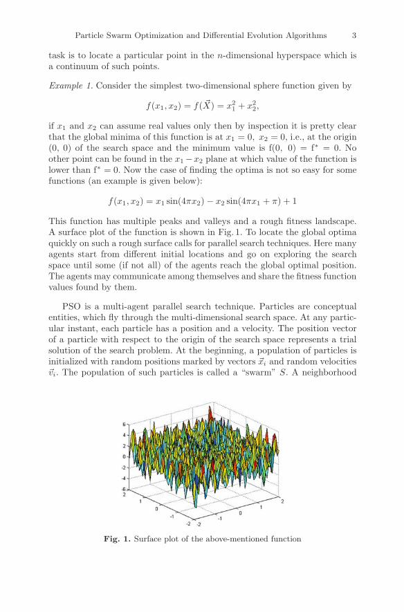
Example 1. Consider the simplest two-dimensional sphere function given by

f(x1, x2) = f( �X) = x21 + x2

2,

if x1 and x2 can assume real values only then by inspection it is pretty clearthat the global minima of this function is at x1 = 0, x2 = 0, i.e., at the origin(0, 0) of the search space and the minimum value is f(0, 0) = f∗ = 0. Noother point can be found in the x1−x2 plane at which value of the function islower than f∗ = 0. Now the case of finding the optima is not so easy for somefunctions (an example is given below):

f(x1, x2) = x1 sin(4πx2) − x2 sin(4πx1 + π) + 1

This function has multiple peaks and valleys and a rough fitness landscape.A surface plot of the function is shown in Fig. 1. To locate the global optimaquickly on such a rough surface calls for parallel search techniques. Here manyagents start from different initial locations and go on exploring the searchspace until some (if not all) of the agents reach the global optimal position.The agents may communicate among themselves and share the fitness functionvalues found by them.

PSO is a multi-agent parallel search technique. Particles are conceptualentities, which fly through the multi-dimensional search space. At any partic-ular instant, each particle has a position and a velocity. The position vectorof a particle with respect to the origin of the search space represents a trialsolution of the search problem. At the beginning, a population of particles isinitialized with random positions marked by vectors �xi and random velocities�vi. The population of such particles is called a “swarm” S. A neighborhood

Fig. 1. Surface plot of the above-mentioned function

4 S. Das et al.

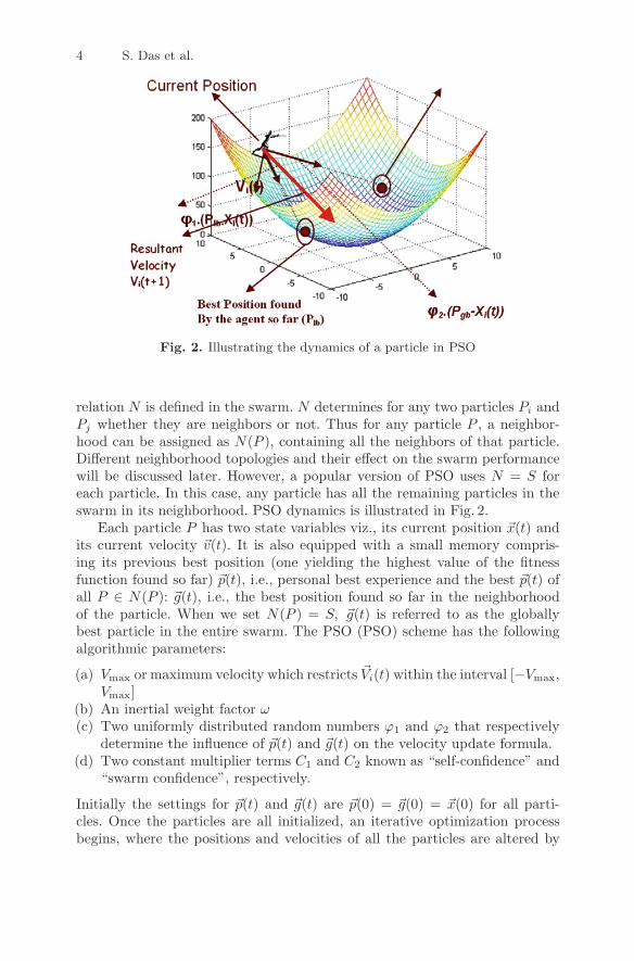
Fig. 2. Illustrating the dynamics of a particle in PSO

relation N is defined in the swarm. N determines for any two particles Pi andPj whether they are neighbors or not. Thus for any particle P , a neighbor-hood can be assigned as N(P ), containing all the neighbors of that particle.Different neighborhood topologies and their effect on the swarm performancewill be discussed later. However, a popular version of PSO uses N = S foreach particle. In this case, any particle has all the remaining particles in theswarm in its neighborhood. PSO dynamics is illustrated in Fig. 2.

Each particle P has two state variables viz., its current position �x(t) andits current velocity �v(t). It is also equipped with a small memory compris-ing its previous best position (one yielding the highest value of the fitnessfunction found so far) �p(t), i.e., personal best experience and the best �p(t) ofall P ∈ N(P ): �g(t), i.e., the best position found so far in the neighborhoodof the particle. When we set N(P ) = S, �g(t) is referred to as the globallybest particle in the entire swarm. The PSO (PSO) scheme has the followingalgorithmic parameters:

(a) Vmax or maximum velocity which restricts �Vi(t) within the interval [−Vmax,Vmax]

(b) An inertial weight factor ω(c) Two uniformly distributed random numbers ϕ1 and ϕ2 that respectively

determine the influence of �p(t) and �g(t) on the velocity update formula.(d) Two constant multiplier terms C1 and C2 known as “self-confidence” and

“swarm confidence”, respectively.

Initially the settings for �p(t) and �g(t) are �p(0) = �g(0) = �x(0) for all parti-cles. Once the particles are all initialized, an iterative optimization processbegins, where the positions and velocities of all the particles are altered by


the following recursive equations. The equations are presented for the dthdimension of the position and velocity of the ith particle.

Vid(t + 1) = ω · vid(t) + C1 · ϕ1 · (Pid(t) − xid(t)) + C2 · ϕ2 · (gid(t) − xid(t))

xid(t + 1) = xid(t) + vid(t + 1).

}(1)

The first term in the velocity updating formula represents the inertial velocityof the particle. “ω” is called the inertia factor. Venter and Sobeiski [10] termedC1 as “self-confidence” and C2 as “swarm confidence”. These terminologiesprovide an insight from a sociological standpoint. Since the coefficient C1 hasa contribution towards the self-exploration (or experience) of a particle, weregard it as the particle’s self-confidence. On the other hand, the coefficientC2 has a contribution towards motion of the particles in global direction,which takes into account the motion of all the particles in the preceding pro-gram iterations, naturally its definition as “swarm confidence” is apparent.ϕ1 and ϕ2 stand for a uniformly distributed random number in the interval[0, 1]. After having calculated the velocities and position for the next timestep t + 1, the first iteration of the algorithm is completed. Typically, thisprocess is iterated for a certain number of time steps, or until some accept-able solution has been found by the algorithm or until an upper limit of CPUusage has been reached. The algorithm can be summarized in the followingpseudo code:

The PSO Algorithm

Input: Randomly initialized position and velocity of the particles: �Xi(0) and�Vi(0)

Output: Position of the approximate global optima �X∗

BeginWhile terminating condition is not reached doBeginfor i = 1 to number of particlesEvaluate the fitness:= f( �Xi);Update �pi and �gi;Adapt velocity of the particle using equations (1);Update the position of the particle;increase i;end whileend

The swarm-dynamics has been presented below using a humanoid agent inplace of a particle on the spherical fitness-landscape.

6 S. Das et al.

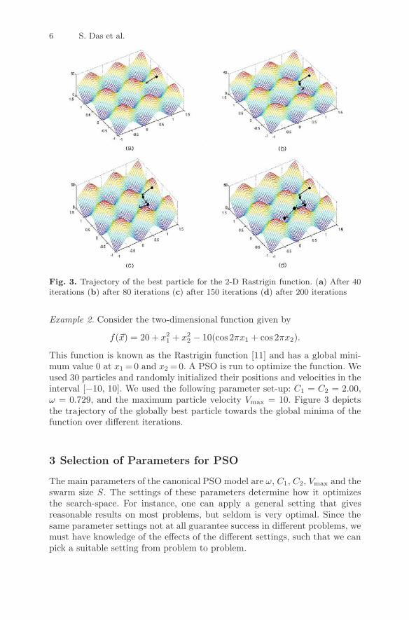
Fig. 3. Trajectory of the best particle for the 2-D Rastrigin function. (a) After 40iterations (b) after 80 iterations (c) after 150 iterations (d) after 200 iterations

Example 2. Consider the two-dimensional function given by

f(�x) = 20 + x21 + x2

2 − 10(cos 2πx1 + cos 2πx2).

This function is known as the Rastrigin function [11] and has a global mini-mum value 0 at x1 =0 and x2 =0. A PSO is run to optimize the function. Weused 30 particles and randomly initialized their positions and velocities in theinterval [−10, 10]. We used the following parameter set-up: C1 = C2 = 2.00,ω = 0.729, and the maximum particle velocity Vmax = 10. Figure 3 depictsthe trajectory of the globally best particle towards the global minima of thefunction over different iterations.

3 Selection of Parameters for PSO

The main parameters of the canonical PSO model are ω, C1, C2, Vmax and theswarm size S. The settings of these parameters determine how it optimizesthe search-space. For instance, one can apply a general setting that givesreasonable results on most problems, but seldom is very optimal. Since thesame parameter settings not at all guarantee success in different problems, wemust have knowledge of the effects of the different settings, such that we canpick a suitable setting from problem to problem.


3.1 The Inertia Weight ω

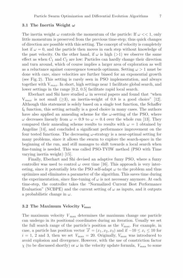
The inertia weight ω controls the momentum of the particle: If ω << 1, onlylittle momentum is preserved from the previous time-step; thus quick changesof direction are possible with this setting. The concept of velocity is completelylost if ω = 0, and the particle then moves in each step without knowledge ofthe past velocity. On the other hand, if ω is high (>1) we observe the sameeffect as when C1 and C2 are low: Particles can hardly change their directionand turn around, which of course implies a larger area of exploration as wellas a reluctance against convergence towards optimum. Setting ω > 1 must bedone with care, since velocities are further biased for an exponential growth(see Fig. 2). This setting is rarely seen in PSO implementation, and alwaystogether with Vmax. In short, high settings near 1 facilitate global search, andlower settings in the range [0.2, 0.5] facilitate rapid local search.

Eberhart and Shi have studied ω in several papers and found that “whenVmax is not small (≥3), an inertia-weight of 0.8 is a good choice” [12].Although this statement is solely based on a single test function, the Schafferf6 function, this setting actually is a good choice in many cases. The authorshave also applied an annealing scheme for the ω-setting of the PSO, whereω decreases linearly from ω = 0.9 to ω = 0.4 over the whole run [13]. Theycompared their annealing scheme results to results with ω = 1 obtained byAngeline [14], and concluded a significant performance improvement on thefour tested functions. The decreasing ω-strategy is a near-optimal setting formany problems, since it allows the swarm to explore the search-space in thebeginning of the run, and still manages to shift towards a local search whenfine-tuning is needed. This was called PSO-TVIW method (PSO with Timevarying inertia weight) [15].

Finally, Eberhart and Shi devised an adaptive fuzzy PSO, where a fuzzycontroller was used to control ω over time [16]. This approach is very inter-esting, since it potentially lets the PSO self-adapt ω to the problem and thusoptimizes and eliminates a parameter of the algorithm. This saves time duringthe experimentation, since fine-tuning of ω is not necessary anymore. At eachtime-step, the controller takes the “Normalized Current Best PerformanceEvaluation” (NCBPE) and the current setting of ω as inputs, and it outputsa probabilistic change in ω.

3.2 The Maximum Velocity Vmax

The maximum velocity V max determines the maximum change one particlecan undergo in its positional coordinates during an iteration. Usually we setthe full search range of the particle’s position as the Vmax. For example, incase, a particle has position vector −→x = (x1, x2, x3) and if −10 ≤ xi ≤ 10 fori = 1, 2 and 3, then we set Vmax = 20. Originally, Vmax was introduced toavoid explosion and divergence. However, with the use of constriction factorχ (to be discussed shortly) or ω in the velocity update formula, Vmax to some

8 S. Das et al.

degree has become unnecessary; at least convergence can be assured withoutit [17]. Thus, some researchers simply do not use Vmax. In spite of this fact,the maximum velocity limitation can still improve the search for optima inmany cases.

3.3 The Constriction Factor χ

In 2002, Clerc and Kennedy proposed an adaptive PSO model [17] that usesa new parameter ‘χ’ called the constriction factor. The model also excludedthe inertia weight ω and the maximum velocity parameter Vmax. The velocityupdate scheme proposed by Clerc can be expressed for the dth dimension ofith particle as:

Vid(t + 1) = χ[Vid(t) + C1 · ϕ1 · (Pid(t) − Xid(t)) + C2 · ϕ2 · (gid(t) − Xid(t))]

Xid(t + 1) = Xid(t) + Vid(t + 1),

}(2)

where,

χ =2∣∣∣4 − ϕ −√

ϕ2 − 4ϕ∣∣∣ With ϕ = C1 + C2

Constriction coefficient results in the quick convergence of the particles overtime. That is the amplitude of a particle’s oscillations decreases as it focuseson the local and neighborhood previous best points. Though the particle con-verges to a point over time, the constriction coefficient also prevents collapseif the right social conditions are in place. The particle will oscillate aroundthe weighted mean of pid and pgd, if the previous best position and the neigh-borhood best position are near each other the particle will perform a localsearch. If the previous best position and the neighborhood best position arefar apart from each other, the particle will perform a more exploratory search(global search). During the search, the neighborhood best position and pre-vious best position will change and the particle will shift from local searchback to global search. The constriction coefficient method therefore balancesthe need for local and global search depending on what social conditions arein place.

3.4 The Swarm Size

It is quite a common practice in the PSO literature to limit the number ofparticles to limit the number of particles to the range 20–60 [12, 18]. Vanden Bergh and Engelbrecht [19] have shown that though there is a slightimprovement of the optimal value with increasing swarm size, a larger swarmincreases the number of function evaluations to converge to an error limit.Eberhart and Shi [18] illustrated that the population size has hardly anyeffect on the performance of the PSO method.


3.5 The Acceleration Coefficients C1 and C2

A usual choice for the acceleration coefficients C1 and C2 is C1 = C2 = 1.494[18]. However, other settings were also used in different papers. Usually C1

equals to C2 and ranges from [0, 4]. Ratnaweera et al. have recently investi-gated the effect of varying these coefficients with time in [20]. Authors adaptedC1 and C2 with time in the following way:

C1 = (C1f − C1i)iter

MAXITER+ C1i

C2 = (C2f − C2i)iter

MAXITER+ C2i

, (3)

where C1i, C1f , C2i, and C2f are constants, iter is the current iteration num-ber and MAXITER is the number of maximum allowable iterations. Theobjective of this modification was to boost the global search over the entiresearch space during the early part of the optimization and to encourage theparticles to converge to global optima at the end of the search. The authorsreferred this as the PSO-TVAC (PSO with time varying acceleration coeffi-cients) method. Actually C1 was decreased from 2.5 to 0.5 whereas C2 wasincreased from 0.5 to 2.5.

4 The Neighborhood Topologies in PSO

The commonly used PSOs are either global version or local version of PSO [5].In the global version of PSO, each particle flies through the search space witha velocity that is dynamically adjusted according to the particle’s personalbest performance achieved so far and the best performance achieved so far byall the particle. While in the local version of PSO, each particle’s velocity isadjusted according to its personal best and the best performance achieved asfar within its neighborhood. The neighborhood of each particle is generallydefined as topologically nearest particles to the particle at each side. Theglobal version of PSO also can be considered as a local version of PSO witheach particle’s neighborhood to be the whole population. It has been suggestedthat the global version of PSO converges fast, but with potential to convergeto the local minimum, while the local version of PSO might have more chancesto find better solutions slowly [5]. Since then, a lot of researchers have workedon improving its performance by designing or implementing different types ofneighborhood structures in PSO. Kennedy [21] claimed that PSO with smallneighborhoods might perform better on complex problems while PSO withlarge neighborhood would perform better for simple problems.

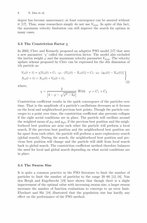
The k-best topology, proposed by Kennedy connects every particle to itsk nearest particles in the topological space. With k = 2, this becomes thecircle topology (and with k = swarmsize-1 it becomes a gbest topology). Thewheel topology, in which the only connections are from one central particle to

10 S. Das et al.

Fig. 4. (a) The fully connected org best topology (b) The k-best nearest neighbortopology with k = 2 and (c) the wheel topology

the others (see Fig. 4). In addition, one could imagine a huge number of othertopologies.

5 The Binary PSO

A binary optimization problem is a (normal) optimization problem, wherethe search space S is simply the set of strings of 0s and 1s of a given fixedlength, n. A binary optimization algorithm solves binary optimization prob-lems, and thus enables us to solve many discrete problems. Hence, faced witha problem-domain that we cannot fit into some sub-space of the real-valuedn-dimensional space, which is required by the PSO, odds are that we canuse a binary PSO instead. All we must provide is a mapping from this givenproblem-domain to the set of bit strings.

The binary PSO model was presented by Kennedy and Eberhart, and isbased on a very simple modification of the real-valued PSO [22]. As with theoriginal PSO, a fitness function f must be defined. In this case, it maps fromthe n-dimensional binary space Bn (i.e., bit strings of length n) to the realnumbers: f : Bn → �n. In the binary PSO the positions of the particlesnaturally must belong to Bn in order to be evaluated by f . Surprisingly,the velocities till belong to V = [−Vmax, Vmin] ⊂ �. This is obtained bychanging the position update formula (1) and leaving the velocity updateformula unchanged. Now, the ith coordinate of each particle’s position is abit, which state is given by

Xi(t + 1) = 1 if ρ < s(�Vi(t)),= 0 otherwise, (4)

where ρ is a random and uniformly selected number in [0, 1], which is re-sampled for each assignment of �Xi(t). S is a sigmoid function that maps fromthe real numbers into [0, 1]. It has the properties that S(0) = 1

2 and S(x) → 0as x → ∞. It is mathematically formulated as

S(x) =1

1 + e−x


The position �Xi(t) has changed from being a point in real-valued space tobeing a bit-string, and the velocity �Vi(t) has now become a probability for�Xi(t) to be 1or 0. If �Vi(t) = 0 the probability for the outcome �Xi(t + 1) = 1will be 50%. On the other hand, if �Vi(t) > 0 the probability for �Xi(t + 1) = 1will be above 50%, and if �Vi(t) < 0 a probability below 50%. It is not quiteclear, at least intuitively, how and why this changed approach will work. Inparticular, to the best of our knowledge, there has not been published anypapers concerning with the changed meaning of the ω parameter in the binaryPSO. The discussion on the meaning of ω above must therefore be regardedas a novel discovery and an independent research result in its own right. Inconclusion, since a binary version of the PSO is a key point to practical andcommercial use of the PSO in discrete problems solving, this topic definitelyneeds a lot more attention in the coming years.

6 Hybridization of PSO with Other EvolutionaryTechniques

A popular research trend is to merge or combine the PSO with the othertechniques, especially the other evolutionary computation techniques. Evolu-tionary operators like selection, crossover and mutation have been applied intothe PSO. By applying selection operation in PSO, the particles with the bestperformance are copied into the next generation; therefore, PSO can alwayskeep the best-performed particles [14]. By applying crossover operation, infor-mation can be swapped between two individuals to have the ability to “fly”to the new search area as that in evolutionary programming and GAs [23].Among the three evolutionary operators, the mutation operators are the mostcommonly applied evolutionary operators in PSO. The purpose of applyingmutation to PSO is to increase the diversity of the population and the abil-ity to have the PSO to escape the local minima [24–27]. One approach is tomutate parameters such as χ, C1 and C2, the position of the neighborhoodbest [26], as well as the inertia weight [25]. Another approach is to preventparticles from moving too close to each other so that the diversity could bemaintained and therefore escape from being trapped into local minima. In [25],the particles are relocated when they are too close to each other. In [24, 27],collision-avoiding mechanisms are designed to prevent particle from collidingwith each other and therefore increase the diversity of the population. In addi-tion to incorporating evolutionary operations into PSO, different approachesto combine PSO with the other evolutionary algorithms have been reported.Robinson et al. [28] obtained better results by applying PSO first followed byapplying GA in their profiled corrugated horn antenna optimization problem.In [29], either PSO algorithm or GA or hill climbing search algorithm canbe applied to a different sub-population of individuals which each individualis dynamically assigned to according to some pre-designed rules. In [30], ant

12 S. Das et al.

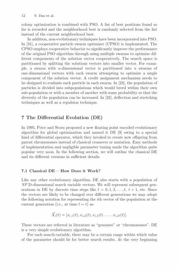
colony optimization is combined with PSO. A list of best positions found sofar is recorded and the neighborhood best is randomly selected from the listinstead of the current neighborhood best.

In addition, non-evolutionary techniques have been incorporated into PSO.In [31], a cooperative particle swarm optimizer (CPSO) is implemented. TheCPSO employs cooperative behavior to significantly improve the performanceof the original PSO algorithm through using multiple swarms to optimize dif-ferent components of the solution vector cooperatively. The search space ispartitioned by splitting the solutions vectors into smaller vector. For exam-ple, a swarm with n-dimensional vector is partitioned into n swarms ofone-dimensional vectors with each swarm attempting to optimize a singlecomponent of the solution vector. A credit assignment mechanism needs tobe designed to evaluate each particle in each swarm. In [23], the population ofparticles is divided into subpopulations which would breed within their ownsub-population or with a member of another with some probability so that thediversity of the population can be increased. In [32], deflection and stretchingtechniques as well as a repulsion technique.

7 The Differential Evolution (DE)

In 1995, Price and Storn proposed a new floating point encoded evolutionaryalgorithm for global optimization and named it DE [9] owing to a specialkind of differential operator, which they invoked to create new offspring fromparent chromosomes instead of classical crossover or mutation. Easy methodsof implementation and negligible parameter tuning made the algorithm quitepopular very soon. In the following section, we will outline the classical DEand its different versions in sufficient details.

7.1 Classical DE – How Does it Work?

Like any other evolutionary algorithm, DE also starts with a population ofNP D-dimensional search variable vectors. We will represent subsequent gen-erations in DE by discrete time steps like t = 0, 1, 2, . . . , t, t + 1, etc. Sincethe vectors are likely to be changed over different generations we may adoptthe following notation for representing the ith vector of the population at thecurrent generation (i.e., at time t = t) as

�Xi(t) = [xi,1(t), xi,2(t), xi,3(t) . . . . . xi,D(t)].

These vectors are referred in literature as “genomes” or “chromosomes”. DEis a very simple evolutionary algorithm.

For each search-variable, there may be a certain range within which valueof the parameter should lie for better search results. At the very beginning


of a DE run or at t = 0, problem parameters or independent variables areinitialized somewhere in their feasible numerical range. Therefore, if the jthparameter of the given problem has its lower and upper bound as xL

j and xUj ,

respectively, then we may initialize the jth component of the ith populationmembers as

xi,j(0) = xLj + rand (0, 1) · (xU

j − xLj ),

where rand (0,1) is a uniformly distributed random number lying between 0and 1.

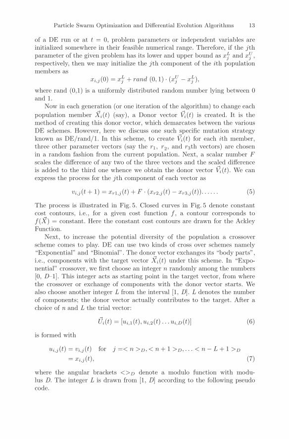
Now in each generation (or one iteration of the algorithm) to change eachpopulation member �Xi(t) (say), a Donor vector �Vi(t) is created. It is themethod of creating this donor vector, which demarcates between the variousDE schemes. However, here we discuss one such specific mutation strategyknown as DE/rand/1. In this scheme, to create �Vi(t) for each ith member,three other parameter vectors (say the r1, r2, and r3th vectors) are chosenin a random fashion from the current population. Next, a scalar number Fscales the difference of any two of the three vectors and the scaled differenceis added to the third one whence we obtain the donor vector �Vi(t). We canexpress the process for the jth component of each vector as

vi,j(t + 1) = xr1,j(t) + F · (xr2,j(t) − xr3,j(t)). . . . . . (5)

The process is illustrated in Fig. 5. Closed curves in Fig. 5 denote constantcost contours, i.e., for a given cost function f , a contour corresponds tof( �X) = constant. Here the constant cost contours are drawn for the AckleyFunction.

Next, to increase the potential diversity of the population a crossoverscheme comes to play. DE can use two kinds of cross over schemes namely“Exponential” and “Binomial”. The donor vector exchanges its “body parts”,i.e., components with the target vector �Xi(t) under this scheme. In “Expo-nential” crossover, we first choose an integer n randomly among the numbers[0, D–1]. This integer acts as starting point in the target vector, from wherethe crossover or exchange of components with the donor vector starts. Wealso choose another integer L from the interval [1, D]. L denotes the numberof components; the donor vector actually contributes to the target. After achoice of n and L the trial vector:

�Ui(t) = [ui,1(t), ui,2(t) . . . ui,D(t)] (6)

is formed with

ui,j(t) = vi,j(t) for j =< n >D, < n + 1 >D, . . . < n − L + 1 >D

= xi,j(t), (7)

where the angular brackets <>D denote a modulo function with modu-lus D. The integer L is drawn from [1, D] according to the following pseudocode.

14 S. Das et al.

Fig. 5. Illustrating creation of the donor vector in 2-D parameter space (Theconstant cost contours are for two-dimensional Ackley Function)

L = 0;do{

L=L+1;} while (rand (0, 1) < CR) AND (L<D));

Hence in effect probability (L > m) = (CR)m−1 for any m > 0. CR is called“Crossover” constant and it appears as a control parameter of DE just likeF. For each donor vector V, a new set of n and L must be chosen randomlyas shown above. However, in “Binomial” crossover scheme, the crossover isperformed on each of the D variables whenever a randomly picked numberbetween 0 and 1 is within the CR value. The scheme may be outlined as

ui,j(t) = vi,j(t) if rand (0, 1) < CR,

= xi,j(t) else... . .. (8)

In this way for each trial vector �Xi(t) an offspring vector �Ui(t) is created. Tokeep the population size constant over subsequent generations, the next stepof the algorithm calls for “selection” to determine which one of the targetvector and the trial vector will survive in the next generation, i.e., at time


t = t + 1. DE actually involves the Darwinian principle of “Survival of thefittest” in its selection process which may be outlined as

�Xi(t + 1) = �Ui(t) if f(�Ui(t)) ≤ f( �Xi(t)),

= �Xi(t) if f( �Xi(t)) < f(�Ui(t)), . . . (9)

where f () is the function to be minimized. So if the new trial vector yields abetter value of the fitness function, it replaces its target in the next generation;otherwise the target vector is retained in the population. Hence the populationeither gets better (w.r.t. the fitness function) or remains constant but neverdeteriorates. The DE/rand/1 algorithm is outlined below:

Procedure DE

Input: Randomly initialized position and velocity of the particles: �xi(0)

Output: Position of the approximate global optima �X∗

Begin

Initialize population;Evaluate fitness;For i= 0 to max-iteration doBeginCreate Difference-Offspring;Evaluate fitness;If an offspring is better than its parentThen replace the parent by offspring in the next generation;End If;

End For;End.

Example 3. This example illustrates the complete searching on the fitnesslandscape of a two-dimensional sphere function by a simple DE. Sphere isperhaps one of the simplest two-dimensional functions and has been chosento provide easy visual depiction of the search process. The function is given by

f(�x) = x21 + x2

2.

As can be easily perceived, the function has only one global minima f∗ = 0 atX∗ = [0, 0]T. We start with a randomly initialized population of five vectorsin the search range [−10, 10]. Initially, these vectors are given by

X1(0) = [5,−9]T

X2(0) = [6, 1]T

X3(0) = [−3, 5]T

X4(0) = [−7, 4]T

X5(0) = [6, 7]T

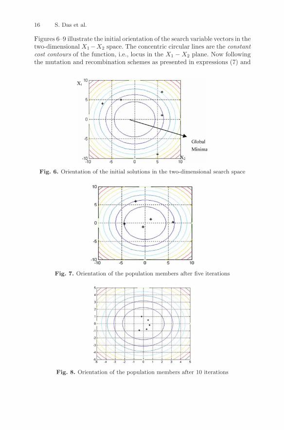
16 S. Das et al.

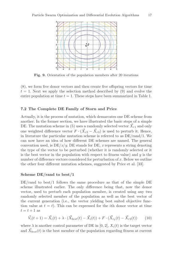
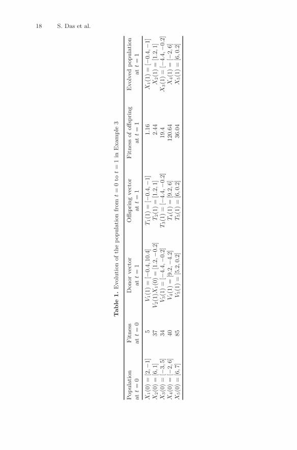
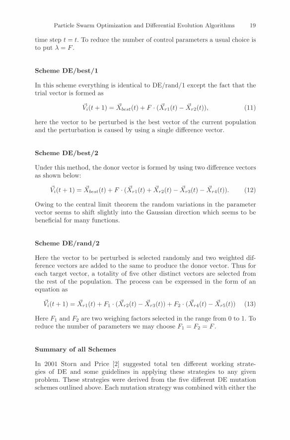
Figures 6–9 illustrate the initial orientation of the search variable vectors in thetwo-dimensional X1−X2 space. The concentric circular lines are the constantcost contours of the function, i.e., locus in the X1 − X2 plane. Now followingthe mutation and recombination schemes as presented in expressions (7) and

Fig. 6. Orientation of the initial solutions in the two-dimensional search space

Fig. 7. Orientation of the population members after five iterations

Fig. 8. Orientation of the population members after 10 iterations


Fig. 9. Orientation of the population members after 20 iterations

(8), we form five donor vectors and then create five offspring vectors for timet = 1. Next we apply the selection method described by (9) and evolve theentire population at time t = 1. These steps have been summarized in Table 1.

7.2 The Complete DE Family of Storn and Price

Actually, it is the process of mutation, which demarcates one DE scheme fromanother. In the former section, we have illustrated the basic steps of a simpleDE. The mutation scheme in (5) uses a randomly selected vector �Xr1 and onlyone weighted difference vector F · ( �Xr2 − �Xr3) is used to perturb it. Hence,in literature the particular mutation scheme is referred to as DE/rand/1. Wecan now have an idea of how different DE schemes are named. The generalconvention used, is DE/x/y. DE stands for DE, x represents a string denotingthe type of the vector to be perturbed (whether it is randomly selected or itis the best vector in the population with respect to fitness value) and y is thenumber of difference vectors considered for perturbation of x. Below we outlinethe other four different mutation schemes, suggested by Price et al. [33].

Scheme DE/rand to best/1

DE/rand to best/1 follows the same procedure as that of the simple DEscheme illustrated earlier. The only difference being that, now the donorvector, used to perturb each population member, is created using any tworandomly selected member of the population as well as the best vector ofthe current generation (i.e., the vector yielding best suited objective func-tion value at t = t). This can be expressed for the ith donor vector at timet = t + 1 as

�Vi(t + 1) = �Xi(t) + λ · ( �Xbest(t) − �Xi(t)) + F · ( �Xr2(t) − �Xr3(t)) (10)

where λ is another control parameter of DE in [0, 2], Xi(t) is the target vectorand �Xbest(t) is the best member of the population regarding fitness at current

18 S. Das et al.

Table

1.

Evolu

tion

ofth

epopula

tion

from

t=

0to

t=

1in

Exam

ple

3

Popula

tion

Fitnes

sD

onor

vec

tor

Offsp

ring

vec

tor

Fitnes

sofoffsp

ring

Evolv

edpopula

tion

at

t=

0at

t=

0at

t=

1at

t=

1at

t=

1at

t=

1

X1(0

)=

[2,−

1]

5V

1(1

)=

[−0.4

,10.4

]T

1(1

)=

[−0.4

,−1]

1.1

6X

1(1

)=

[−0.4

,−1]

X2(0

)=

[6,1

]37

V2(1

)X1(0

)=

[1.2

,−0.2

]T

2(1

)=

[1.2

,1]

2.4

4X

2(1

)=

[1.2

,1]

X3(0

)=

[−3,5

]34

V3(1

)=

[−4.4

,−0.2

]T

3(1

)=

[−4.4

,−0.2

]19.4

X3(1

)=

[−4.4

,−0.2

]X

4(0

)=

[−2,6

]40

V4(1

)=

[9.2

,−4.2

]T

4(1

)=

[9.2

,6]

120.6

4X

4(1

)=

[−2,6

]X

5(0

)=

[6,7

]85

V5(1

)=

[5.2

,0.2

]T

5(1

)=

[6,0

.2]

36.0

4X

5(1

)=

[6,0

.2]


time step t = t. To reduce the number of control parameters a usual choice isto put λ = F .

Scheme DE/best/1

In this scheme everything is identical to DE/rand/1 except the fact that thetrial vector is formed as

�Vi(t + 1) = �Xbest(t) + F · ( �Xr1(t) − �Xr2(t)), (11)

here the vector to be perturbed is the best vector of the current populationand the perturbation is caused by using a single difference vector.

Scheme DE/best/2

Under this method, the donor vector is formed by using two difference vectorsas shown below:

�Vi(t + 1) = �Xbest(t) + F · ( �Xr1(t) + �Xr2(t) − �Xr3(t) − �Xr4(t)). (12)

Owing to the central limit theorem the random variations in the parametervector seems to shift slightly into the Gaussian direction which seems to bebeneficial for many functions.

Scheme DE/rand/2

Here the vector to be perturbed is selected randomly and two weighted dif-ference vectors are added to the same to produce the donor vector. Thus foreach target vector, a totality of five other distinct vectors are selected fromthe rest of the population. The process can be expressed in the form of anequation as

�Vi(t + 1) = �Xr1(t) + F1 · ( �Xr2(t) − �Xr3(t)) + F2 · ( �Xr4(t) − �Xr5(t)) (13)

Here F1 and F2 are two weighing factors selected in the range from 0 to 1. Toreduce the number of parameters we may choose F1 = F2 = F .

Summary of all Schemes

In 2001 Storn and Price [2] suggested total ten different working strate-gies of DE and some guidelines in applying these strategies to any givenproblem. These strategies were derived from the five different DE mutationschemes outlined above. Each mutation strategy was combined with either the

20 S. Das et al.

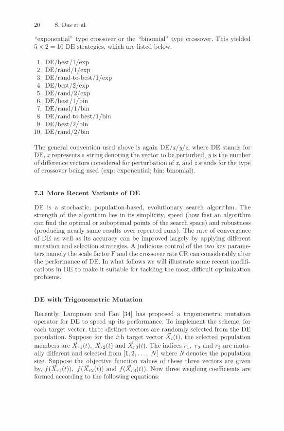
“exponential” type crossover or the “binomial” type crossover. This yielded5 × 2 = 10 DE strategies, which are listed below.

1. DE/best/1/exp2. DE/rand/1/exp3. DE/rand-to-best/1/exp4. DE/best/2/exp5. DE/rand/2/exp6. DE/best/1/bin7. DE/rand/1/bin8. DE/rand-to-best/1/bin9. DE/best/2/bin

10. DE/rand/2/bin

The general convention used above is again DE/x/y/z, where DE stands forDE, x represents a string denoting the vector to be perturbed, y is the numberof difference vectors considered for perturbation of x, and z stands for the typeof crossover being used (exp: exponential; bin: binomial).

7.3 More Recent Variants of DE

DE is a stochastic, population-based, evolutionary search algorithm. Thestrength of the algorithm lies in its simplicity, speed (how fast an algorithmcan find the optimal or suboptimal points of the search space) and robustness(producing nearly same results over repeated runs). The rate of convergenceof DE as well as its accuracy can be improved largely by applying differentmutation and selection strategies. A judicious control of the two key parame-ters namely the scale factor F and the crossover rate CR can considerably alterthe performance of DE. In what follows we will illustrate some recent modifi-cations in DE to make it suitable for tackling the most difficult optimizationproblems.

DE with Trigonometric Mutation

Recently, Lampinen and Fan [34] has proposed a trigonometric mutationoperator for DE to speed up its performance. To implement the scheme, foreach target vector, three distinct vectors are randomly selected from the DEpopulation. Suppose for the ith target vector �Xi(t), the selected populationmembers are �Xr1(t), �Xr2(t) and �Xr3(t). The indices r1, r2 and r3 are mutu-ally different and selected from [1, 2, . . . , N ] where N denotes the populationsize. Suppose the objective function values of these three vectors are givenby, f( �Xr1(t)), f( �Xr2(t)) and f( �Xr3(t)). Now three weighing coefficients areformed according to the following equations:


p′ =∣∣∣f( �Xr1)

∣∣∣ +∣∣∣f( �Xr2)

∣∣∣ +∣∣∣f( �Xr3)

∣∣∣ , (14)

p1 =∣∣∣f( �Xr1)

∣∣∣/p′, (15)

p2 =∣∣∣f( �Xr2)

∣∣∣/p′, (16)

p3 =∣∣∣f( �Xr3)

∣∣∣/p′. (17)

Let rand (0, 1) be a uniformly distributed random number in (0, 1) and Γ bethe trigonometric mutation rate in the same interval (0, 1). The trigonometricmutation scheme may now be expressed as

�Vi(t + 1) = ( �Xr1 + �Xr2 + �Xr3)/3 + (p2 − p1) · ( �Xr1 − �Xr2)

+ (p3 − p2) · ( �Xr2 − �Xr3) + (p1 − p3) · ( �Xr3 − �Xr1)if rand (0, 1) < Γ

�Vi(t + 1) = �Xr1 + F · ( �Xr2 + �Xr3) else. (18)

Thus, we find that the scheme proposed by Lampinen et al. uses trigonometricmutation with a probability of Γ and the mutation scheme of DE/rand/1 witha probability of (1 − Γ).

DERANDSF (DE with Random Scale Factor)

In the original DE [9] the difference vector ( �Xr1(t) − �Xr2(t)) is scaled by aconstant factor “F ”. The usual choice for this control parameter is a numberbetween 0.4 and 1. We propose to vary this scale factor in a random mannerin the range (0.5, 1) by using the relation

F = 0.5∗(1 + rand (0, 1)), (19)

where rand (0, 1) is a uniformly distributed random number within the range[0, 1]. We call this scheme DERANDSF (DE with Random Scale Factor) [35].The mean value of the scale factor is 0.75. This allows for stochastic variationsin the amplification of the difference vector and thus helps retain populationdiversity as the search progresses. Even when the tips of most of the populationvectors point to locations clustered near a local optimum due to the randomlyscaled difference vector, a new trial vector has fair chances of pointing atan even better location on the multimodal functional surface. Therefore, thefitness of the best vector in a population is much less likely to get stagnantuntil a truly global optimum is reached.

DETVSF (DE with Time Varying Scale Factor)

In most population-based optimization methods (except perhaps some hybridglobal-local methods) it is generally believed to be a good idea to encourage

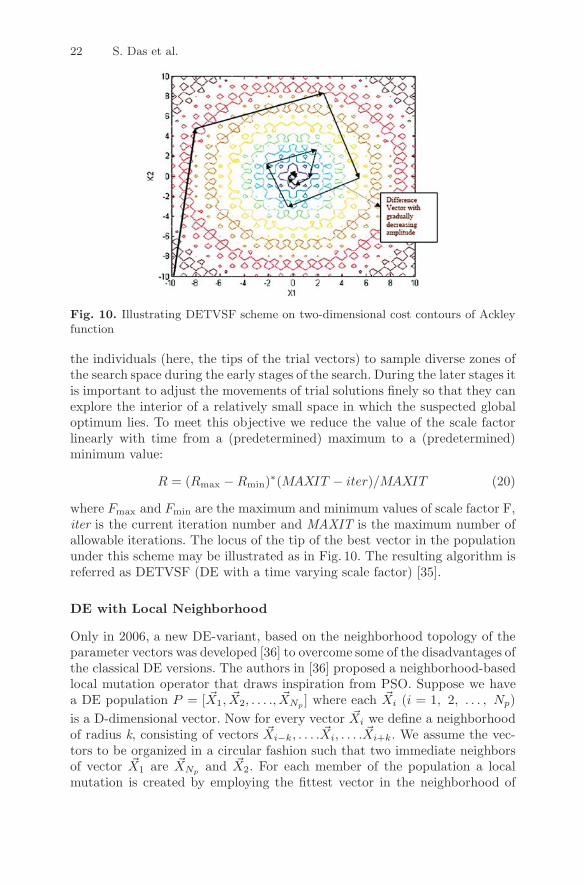
22 S. Das et al.

Fig. 10. Illustrating DETVSF scheme on two-dimensional cost contours of Ackleyfunction

the individuals (here, the tips of the trial vectors) to sample diverse zones ofthe search space during the early stages of the search. During the later stages itis important to adjust the movements of trial solutions finely so that they canexplore the interior of a relatively small space in which the suspected globaloptimum lies. To meet this objective we reduce the value of the scale factorlinearly with time from a (predetermined) maximum to a (predetermined)minimum value:

R = (Rmax − Rmin)∗(MAXIT − iter)/MAXIT (20)

where Fmax and Fmin are the maximum and minimum values of scale factor F,iter is the current iteration number and MAXIT is the maximum number ofallowable iterations. The locus of the tip of the best vector in the populationunder this scheme may be illustrated as in Fig. 10. The resulting algorithm isreferred as DETVSF (DE with a time varying scale factor) [35].

DE with Local Neighborhood

Only in 2006, a new DE-variant, based on the neighborhood topology of theparameter vectors was developed [36] to overcome some of the disadvantages ofthe classical DE versions. The authors in [36] proposed a neighborhood-basedlocal mutation operator that draws inspiration from PSO. Suppose we havea DE population P = [ �X1, �X2, . . . ., �XNp ] where each �Xi (i = 1, 2, . . . , Np)is a D-dimensional vector. Now for every vector �Xi we define a neighborhoodof radius k, consisting of vectors �Xi−k, . . . . �Xi, . . . . �Xi+k. We assume the vec-tors to be organized in a circular fashion such that two immediate neighborsof vector �X1 are �XNp and �X2. For each member of the population a localmutation is created by employing the fittest vector in the neighborhood of


that member and two other vectors chosen from the same neighborhood. Themodel may be expressed as:

�Li(t) = �Xi(t) + λ′ · ( �Xnbest(t) − �Xi(t)) + F ′ · ( �Xp(t) − �Xq(t)) (21)

where the subscript nbest indicates the best vector in the neighborhood of−→X i and p, q ∈ (i − k, i + k). Apart from this, we also use a global mutationexpressed as:

�Gi(t) = �Xi(t) + λ · ( �Xbest(t) − �Xi(t)) + F · ( �Xr(t) − �Xs(t)), (22)

where the subscript best indicates the best vector in the entire population,and r, s ∈ (1, Np). Global mutation encourages exploitation, since all members(vectors) of a population are biased by the same individual (the populationbest); local mutation, in contrast, favors exploration, since in general differentmembers of the population are likely to be biased by different individuals. Nowwe combine these two models using a time-varying scalar weight w ∈ (0, 1) toform the actual mutation of the new DE as a weighted mean of the local andthe global components:

�Vi(t) = w · �Gi(t) + (1 − w) · �Li(t). (23)

The weight factor varies linearly with time as folows:

w = wmin + (wmax − wmin) ·(

iter

MAXIT

), (24)

where iter is the current iteration number, MAXIT is the maximum numberof iterations allowed and wmax, wmin denote, respectively, the maximum andminimum value of the weight, with wmax, wmin ∈ (0, 1). Thus the algorithmstarts at iter = 0 with w = wmin but as iter increases towards MAXIT,w increases gradually and ultimately when iter = MAXIT w reaches wmax.Therefore at the beginning, emphasis is laid on the local mutation scheme, butwith time, contribution from the global model increases. In the local modelattraction towards a single point of the search space is reduced, helping DEavoid local optima. This feature is essential at the beginning of the searchprocess when the candidate vectors are expected to explore the search spacevigorously. Clearly, a judicious choice of wmax and wmin is necessary to strikea balance between the exploration and exploitation abilities of the algorithm.After some experimenting, it was found that wmax = 0.8 and wmin = 0.4 seemto improve the performance of the algorithm over a number of benchmarkfunctions.

8 A Synergism of PSO and DE – Towards a New HybridEvolutionary Algorithm

Das et al. proposed a new scheme of adjusting the velocities of the particlesin PSO with a vector differential operator borrowed from the DE family [37].The canonical PSO updates the velocity of a particle using three terms. These

24 S. Das et al.

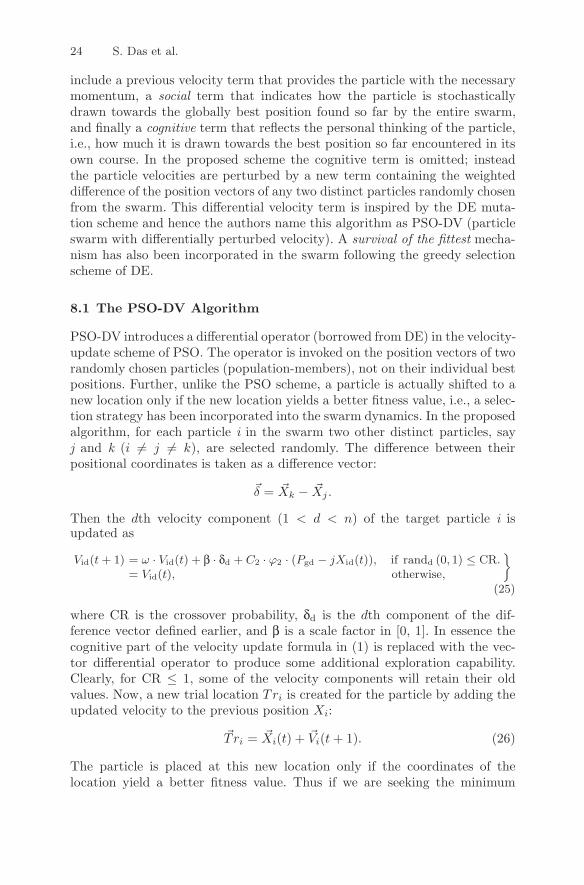
include a previous velocity term that provides the particle with the necessarymomentum, a social term that indicates how the particle is stochasticallydrawn towards the globally best position found so far by the entire swarm,and finally a cognitive term that reflects the personal thinking of the particle,i.e., how much it is drawn towards the best position so far encountered in itsown course. In the proposed scheme the cognitive term is omitted; insteadthe particle velocities are perturbed by a new term containing the weighteddifference of the position vectors of any two distinct particles randomly chosenfrom the swarm. This differential velocity term is inspired by the DE muta-tion scheme and hence the authors name this algorithm as PSO-DV (particleswarm with differentially perturbed velocity). A survival of the fittest mecha-nism has also been incorporated in the swarm following the greedy selectionscheme of DE.

8.1 The PSO-DV Algorithm

PSO-DV introduces a differential operator (borrowed from DE) in the velocity-update scheme of PSO. The operator is invoked on the position vectors of tworandomly chosen particles (population-members), not on their individual bestpositions. Further, unlike the PSO scheme, a particle is actually shifted to anew location only if the new location yields a better fitness value, i.e., a selec-tion strategy has been incorporated into the swarm dynamics. In the proposedalgorithm, for each particle i in the swarm two other distinct particles, sayj and k (i �= j �= k), are selected randomly. The difference between theirpositional coordinates is taken as a difference vector:

�δ = �Xk − �Xj .

Then the dth velocity component (1 < d < n) of the target particle i isupdated as

Vid(t + 1) = ω · Vid(t) + β · δd + C2 · ϕ2 · (Pgd − jXid(t)), if randd (0, 1) ≤ CR.= Vid(t), otherwise,

}(25)

where CR is the crossover probability, δd is the dth component of the dif-ference vector defined earlier, and β is a scale factor in [0, 1]. In essence thecognitive part of the velocity update formula in (1) is replaced with the vec-tor differential operator to produce some additional exploration capability.Clearly, for CR ≤ 1, some of the velocity components will retain their oldvalues. Now, a new trial location Tri is created for the particle by adding theupdated velocity to the previous position Xi:

�Tri = �Xi(t) + �Vi(t + 1). (26)

The particle is placed at this new location only if the coordinates of thelocation yield a better fitness value. Thus if we are seeking the minimum


of an n-dimensional function f( �X), then the target particle is relocated asfollows:

�Xi(t + 1) = �Tri if f(�Tri) ≤ f( �Xi(t)),�Xi(t + 1) = �Xi(t) Otherwise,

(27)

Therefore, every time its velocity changes, the particle either moves to a betterposition in the search space or sticks to its previous location. The currentlocation of the particle is thus the best location it has ever found. In otherwords, unlike the classical PSO, in the present scheme, Plid always equalsXid. So the cognitive part involving |Plid − Xid| is automatically eliminatedin our algorithm. If a particle gets stagnant at any point in the search space(i.e., if its location does not change for a predetermined number of iterations),then the particle is shifted by a random mutation (explained below) to a newlocation. This technique helps escape local minima and also keeps the swarm“moving”:

If ( �Xi(t) = �Xi(t + 1) = �Xi(t + 2) = . . . . = �Xi(t + N)) and f( �Xi(t + N))then

for (r = 1 to n)Xir(t + N + 1) = Xmin + randr (0, 1)∗(Xmax − Xmin), (28)

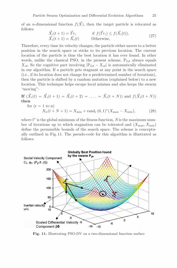
where f∗ is the global minimum of the fitness function, N is the maximum num-ber of iterations up to which stagnation can be tolerated and (Xmax, Xmin)define the permissible bounds of the search space. The scheme is conceptu-ally outlined in Fig. 11. The pseudo-code for this algorithm is illustrated asfollows:

Fig. 11. Illustrating PSO-DV on a two-dimensional function surface

26 S. Das et al.

Procedure PSO-DV

begininitialize population;

while stopping condition not satisfied dofor i = 1 to no of particlesevaluate fitness of particle;update Pgd;select two other particles j and k (i �= j �= k) randomly;construct the difference vector as �δ = �Xk − �Xj;for d = 1 to no of dimensions

if randd (0, 1) ≤ CRVid(t + 1) = ω · Vid(t) + β · δd + C2 · ϕ2 · (Pgd − Xid(t));

else Vid(t + 1) = Vid(t);endif

endforcreate trial location as �Tri = �Xi(t) + �Vi(t + 1);

if (f(�Tri) ≤ f( �Xi(t))) then �Xi(t + 1) = �Tr;else �Xi(t + 1) = �Xi(t);endif

endforfor i = 1 to no of particles

if Xi stagnates for N successive generationsfor r = 1 to no of dimensionsXir(t + 1) = Xmin + randr (0, 1)∗(Xmax − Xmin)end for

end ifend for

end whileend

9 PSO-DV Versus Other State-of-the-Art Optimizers

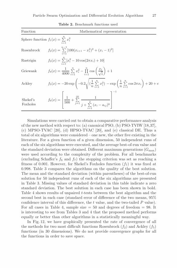
In this section we provide performance comparison between PSO-DV andfour variants of the PSO algorithm and the classical DE algorithm over atest-bed of five well known benchmark functions. In Table 2, n represents thenumber of dimensions (we used n = 25, 50, 75 and 100). The first two testfunctions are uni-modal, having only one minimum. The others are multi-modal, with a considerable number of local minima in the region of interest.All benchmark functions except f6 have the global minimum at the origin orvery near to the origin [28]. For Shekel’s foxholes (f6), the global minimum isat (−31.95, −31.95) and f6 (−31.95, −31.95) ≈ 0.998, and the function hasonly two dimensions. An asymmetrical initialization procedure has been usedhere following the work reported in [29].


Table 2. Benchmark functions used

Function Mathematical representation

Sphere function f1(x) =n∑

i=1

x2i

Rosenbrock f2(x) =n−1∑i=1

[100(xi+1 − x2i )

2 + (xi − 1)2]

Rastrigin f3(x) =n∑

i=1

[x2i − 10 cos(2πxi) + 10]

Griewank f4(x) =1

4000

n∑i=1

x2i −

n∏i=1

cos

(xi√

i

)+ 1

Ackley f5(x) = −20 exp

(−0.2

√(1

n

n∑i=1

x2i ) − exp

(1

n

n∑i=1

cos 2πxi

)+ 20 + e

Shekel’sFoxholes

f6(x) =

⎡⎢⎢⎣ 1

500+

25∑j=1

1

j +2∑

i=1

(xi − aij)6

⎤⎥⎥⎦−1

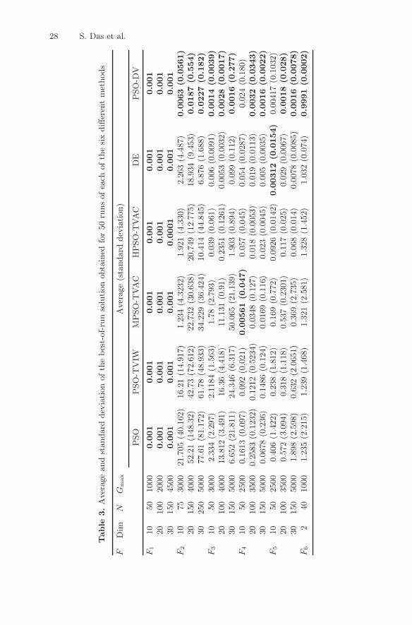
Simulations were carried out to obtain a comparative performance analysisof the new method with respect to: (a) canonical PSO, (b) PSO-TVIW [18,37],(c) MPSO-TVAC [20], (d) HPSO-TVAC [20], and (e) classical DE. Thus atotal of six algorithms were considered – one new, the other five existing in theliterature. For a given function of a given dimension, 50 independent runs ofeach of the six algorithms were executed, and the average best-of-run value andthe standard deviation were obtained. Different maximum generations (Gmax)were used according to the complexity of the problem. For all benchmarks(excluding Schaffer’s f6 and f7) the stopping criterion was set as reaching afitness of 0.001. However, for Shekel’s Foxholes function (f7) it was fixed at0.998. Table 3 compares the algorithms on the quality of the best solution.The mean and the standard deviation (within parentheses) of the best-of-runsolution for 50 independent runs of each of the six algorithms are presentedin Table 3. Missing values of standard deviation in this table indicate a zerostandard deviation. The best solution in each case has been shown in bold.Table 4 shows results of unpaired t-tests between the best algorithm and thesecond best in each case (standard error of difference of the two means, 95%confidence interval of this difference, the t value, and the two-tailed P value).For all cases in Table 4, sample size = 50 and degrees of freedom = 98. Itis interesting to see from Tables 3 and 4 that the proposed method performsequally or better than other algorithms in a statistically meaningful way.

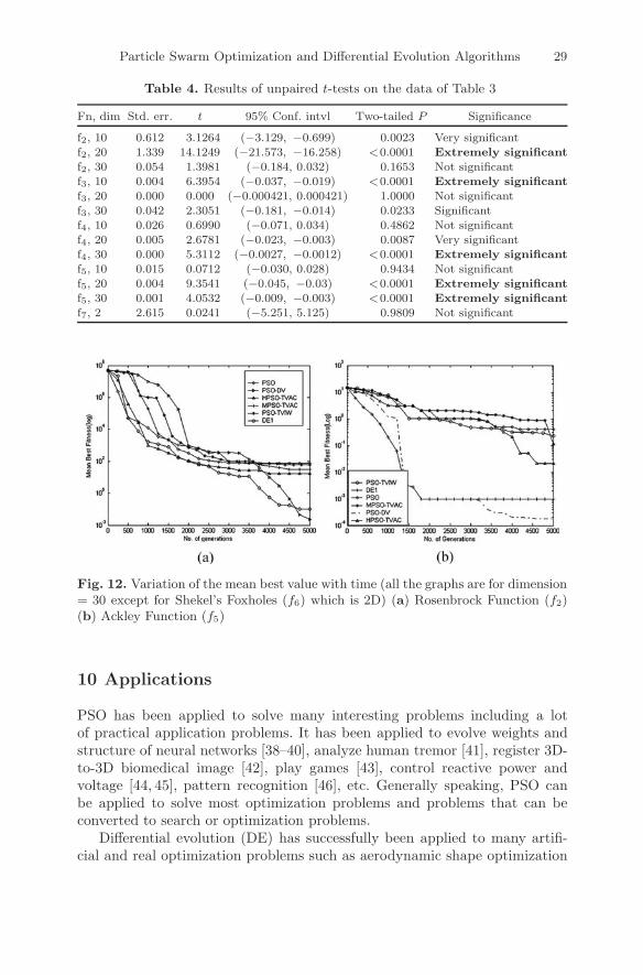
In Fig. 12, we have graphically presented the rate of convergence of allthe methods for two most difficult functions Rosenbrock (f2) and Ackley (f5)functions (in 30 dimensions). We do not provide convergence graphs for allthe functions in order to save space.

28 S. Das et al.

Table

3.

Aver

age

and

standard

dev

iation

ofth

ebes

t-of-ru

nso

lution

obta

ined

for

50

runs

ofea

chofth

esix

diff

eren

tm

ethods

FD

imN

Gm

ax

Aver

age

(sta

ndard

dev

iation)

PSO

PSO

-TV

IWM

PSO

-TVA

CH

PSO

-TVA

CD

EP

SO

-DV

F1

10

50

1000

0.0

01

0.0

01

0.0

01

0.0

01

0.0

01

0.0

01

20

100

2000

0.0

01

0.0

01

0.0

01

0.0

01

0.0

01

0.0

01

30

150

4500

0.0

01

0.0

01

0.0

01

0.0

001

0.0

01

0.0

01

F2

10

75

3000

21.7

05

(40.1

62)

16.2

1(1

4.9

17)

1.2

34

(4.3

232)

1.9

21

(4.3

30)

2.2

63

(4.4

87)

0.0

063

(0.0

561)

20

150

4000

52.2

1(1

48.3

2)

42.7

3(7

2.6

12)

22.7

32

(30.6

38)

20.7

49

(12.7

75)

18.9

34

(9.4

53)

0.0

187

(0.5

54)

30

250

5000

77.6

1(8

1.1

72)

61.7

8(4

8.9

33)

34.2

29

(36.4

24)

10.4

14

(44.8

45)

6.8

76

(1.6

88)

0.0

227

(0.1

82)

F3

10

50

3000

2.3

34

(2.2

97)

2.1

184

(1.5

63)

1.7

8(2

.793)

0.0

39

(0.0

61)

0.0

06

(0.0

091)

0.0

014

(0.0

039)

20

100

4000

13.8

12

(3.4

91)

16.3

6(4

.418)

11.1

31

(0.9

1)

0.2

351

(0.1

261)

0.0

053

(0.0

032)

0.0

028

(0.0

017)

30

150

5000

6.6

52

(21.8

11)

24.3

46

(6.3

17)

50.0

65

(21.1

39)

1.9

03

(0.8

94)

0.0

99

(0.1

12)

0.0

016

(0.2

77)

F4

10

50

2500

0.1

613

(0.0

97)

0.0

92

(0.0

21)

0.0

0561

(0.0

47)

0.0

57

(0.0

45)

0.0

54

(0.0

287)

0.0

24

(0.1

80)

20

100

3500

0.2

583

(0.1

232)

0.1

212

(0.5

234)

0.0

348

(0.1

27)

0.0

18

(0.0

053)

0.0

19

(0.0

113)

0.0

032

(0.0

343)

30

150

5000

0.0

678

(0.2

36)

0.1

486

(0.1

24)

0.0

169

(0.1

16)

0.0

23

(0.0

045)

0.0

05

(0.0

035)

0.0

016

(0.0

022)

F5

10

50

2500

0.4

06

(1.4

22)

0.2

38

(1.8

12)

0.1

69

(0.7

72)

0.0

926

(0.0

142)

0.0

0312

(0.0

154)

0.0

0417

(0.1

032)

20

100

3500

0.5

72

(3.0

94)

0.3

18

(1.1

18)

0.5

37

(0.2

301)

0.1

17

(0.0

25)

0.0

29

(0.0

067)

0.0

018

(0.0

28)

30

150

5000

1.8

98

(2.5

98)

0.6

32

(2.0

651)

0.3

69

(2.7

35)

0.0

68

(0.0

14)

0.0

078

(0.0

085)

0.0

016

(0.0

078)

F6

240

1000

1.2

35

(2.2

15)

1.2

39

(1.4

68)

1.3

21

(2.5

81)

1.3

28

(1.4

52)

1.0

32

(0.0

74)

0.9

991

(0.0

002)


Table 4. Results of unpaired t-tests on the data of Table 3

Fn, dim Std. err. t 95% Conf. intvl Two-tailed P Significance

f2, 10 0.612 3.1264 (−3.129, −0.699) 0.0023 Very significantf2, 20 1.339 14.1249 (−21.573, −16.258) <0.0001 Extremely significantf2, 30 0.054 1.3981 (−0.184, 0.032) 0.1653 Not significantf3, 10 0.004 6.3954 (−0.037, −0.019) <0.0001 Extremely significantf3, 20 0.000 0.000 (−0.000421, 0.000421) 1.0000 Not significantf3, 30 0.042 2.3051 (−0.181, −0.014) 0.0233 Significantf4, 10 0.026 0.6990 (−0.071, 0.034) 0.4862 Not significantf4, 20 0.005 2.6781 (−0.023, −0.003) 0.0087 Very significantf4, 30 0.000 5.3112 (−0.0027, −0.0012) <0.0001 Extremely significantf5, 10 0.015 0.0712 (−0.030, 0.028) 0.9434 Not significantf5, 20 0.004 9.3541 (−0.045, −0.03) <0.0001 Extremely significantf5, 30 0.001 4.0532 (−0.009, −0.003) <0.0001 Extremely significantf7, 2 2.615 0.0241 (−5.251, 5.125) 0.9809 Not significant

Fig. 12. Variation of the mean best value with time (all the graphs are for dimension= 30 except for Shekel’s Foxholes (f6) which is 2D) (a) Rosenbrock Function (f2)(b) Ackley Function (f5)

10 Applications

PSO has been applied to solve many interesting problems including a lotof practical application problems. It has been applied to evolve weights andstructure of neural networks [38–40], analyze human tremor [41], register 3D-to-3D biomedical image [42], play games [43], control reactive power andvoltage [44, 45], pattern recognition [46], etc. Generally speaking, PSO canbe applied to solve most optimization problems and problems that can beconverted to search or optimization problems.

Differential evolution (DE) has successfully been applied to many artifi-cial and real optimization problems such as aerodynamic shape optimization

30 S. Das et al.

[47], automated mirror design [48], optimization of radial active magneticbearings [49], and optimization of fermentation by using a high ethanol-tolerance yeast [50]. A DE based neural network-training algorithm was firstintroduced in [51]. In [52] the method’s characteristics as a global optimizerwere compared to other neural network training methods. Das et al. in [53]have compared the performance of some variants of the DE with other com-mon optimization algorithms like PSO, GA, etc. in context to the partitionalclustering problem and concluded in their study that DE rather than GAsshould receive primary attention in such partitional cluster algorithms.

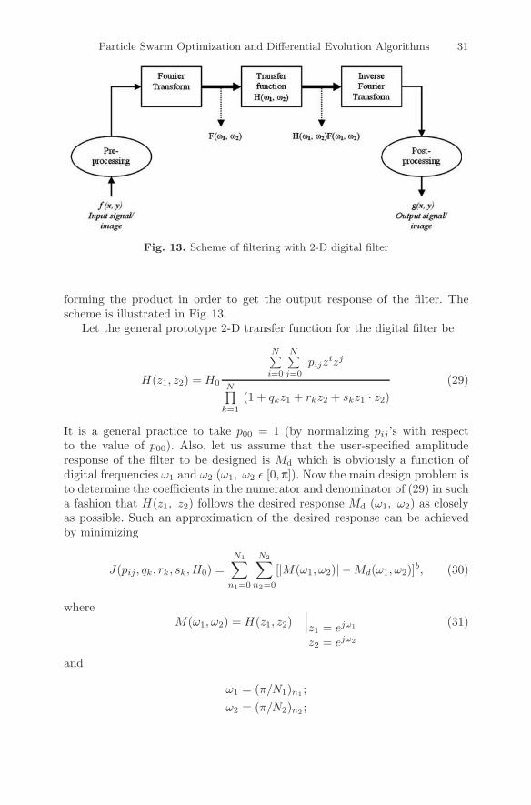
In this section we describe a simple application of the aforementioned algo-rithms to the design of two dimensional IIR filters [54]. In signal processing,the function of a filter is to remove unwanted parts of the signal, such asrandom noise, or to extract useful parts of the signal, such as the componentslying within a certain frequency range. There are two main kinds of filter,analog and digital. They are quite different in their physical makeup and inhow they work. An analog filter uses analog electronic circuits made up fromcomponents such as resistors, capacitors and op-amps to produce the requiredfiltering effect. Such filter circuits are widely used in such applications as noisereduction, video signal enhancement, graphic equalisers in hi-fi systems, andmany other areas. A digital filter uses a digital processor to perform numer-ical calculations on sampled values of the signal. The processor may be ageneral-purpose computer such as a PC, or a specialised DSP (digital signalprocessor) chip.

Digital filters are broadly classified into two main categories namely, FIR(finite impulse response) filters and IIR (infinite impulse response) filters. Theimpulse response of a digital filter is the output sequence from the filter whena unit impulse is applied at its input. (A unit impulse is a very simple inputsequence consisting of a single value of 1 at time t = 0, followed by zeros at allsubsequent sampling instants). An FIR filter is one whose impulse responseis of finite duration. The output of such a filter is calculated solely from thecurrent and previous input values. This type of filter is hence said to be non-recursive. On the other hand, an IIR filter is one whose impulse response(theoretically) continues for ever in time. They are also termed as recursivefilters. The current output of such a filter depends upon previous outputvalues. These, like the previous input values, are stored in the processor’smemory. The word recursive literally means “running back”, and refers to thefact that previously-calculated output values go back into the calculation ofthe latest output. The recursive (previous output) terms feed back energy intothe filter input and keep it going.

In our work [54, 55] the filter design is mainly considered from a fre-quency domain perspective. Frequency domain filtering consists in first, takingthe fourier transform of the two-dimensional signal (which may be the pixelintensity value in case of a gray-scale image), then multiplying the frequencydomain signal by the transfer function of the filter and finally inverse trans-


Fig. 13. Scheme of filtering with 2-D digital filter

forming the product in order to get the output response of the filter. Thescheme is illustrated in Fig. 13.

Let the general prototype 2-D transfer function for the digital filter be

H(z1, z2) = H0

N∑i=0

N∑j=0

pijzizj

N∏k=1

(1 + qkz1 + rkz2 + skz1 · z2)(29)

It is a general practice to take p00 = 1 (by normalizing pij ’s with respectto the value of p00). Also, let us assume that the user-specified amplituderesponse of the filter to be designed is Md which is obviously a function ofdigital frequencies ω1 and ω2 (ω1, ω2 ε [0, π]). Now the main design problem isto determine the coefficients in the numerator and denominator of (29) in sucha fashion that H(z1, z2) follows the desired response Md (ω1, ω2) as closelyas possible. Such an approximation of the desired response can be achievedby minimizing

J(pij , qk, rk, sk, H0) =N1∑

n1=0

N2∑n2=0

[|M(ω1, ω2)| − Md(ω1, ω2)]b, (30)

whereM(ω1, ω2) = H(z1, z2)

∣∣∣z1 = ejω1

z2 = ejω2

(31)

and

ω1 = (π/N1)n1 ;ω2 = (π/N2)n2 ;

32 S. Das et al.

and b is an even positive integer (usually b = 2 or 4). Equation (30) can berestated as

J =N1∑

n1=0

N2∑n2=0

[∣∣∣∣M (πn1

N1,πn2

N2

)∣∣∣∣− Md

(πn1

N1,πn2

N2

)]b

. (32)

Here the prime objective is to reduce the difference between the desired andactual amplitude responses of the filter at N1 ·N2 points. For BIBO (boundedinput bounded output) stability the prime requirement is that the z-planepoles of the filter transfer function should lie within the unit circle. Sincethe denominator contains only first degree factors, we can assert the stabilityconditions as

|qk + rk| − 1 < sk < 1 − |qk − rk|, (33)

where k = 1, 2, . . . , N .We solve the above constrained minimization problems using a binary

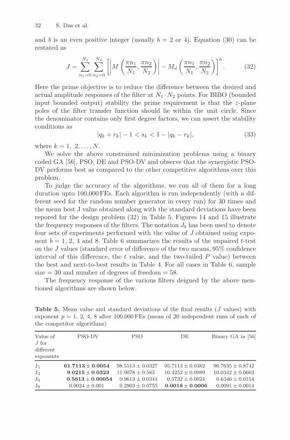
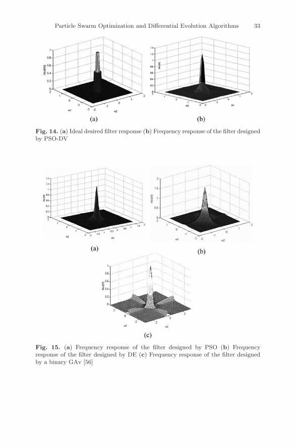
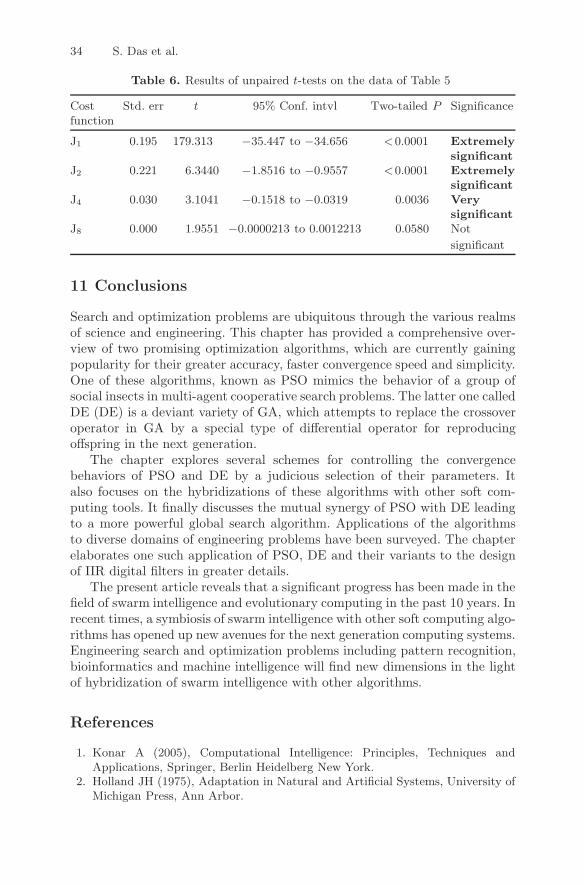
coded GA [56], PSO, DE and PSO-DV and observe that the synergistic PSO-DV performs best as compared to the other competitive algorithms over thisproblem.

To judge the accuracy of the algorithms, we run all of them for a longduration upto 100,000FEs. Each algorithm is run independently (with a dif-ferent seed for the random number generator in every run) for 30 times andthe mean best J value obtained along with the standard deviations have beenrepored for the design problem (32) in Table 5. Figures 14 and 15 illustratethe frequency responses of the filters. The notation Jb has been used to denotefour sets of experiments performed with the value of J obtained using expo-nent b = 1, 2, 4 and 8. Table 6 summarizes the results of the unpaired t-teston the J values (standard error of difference of the two means, 95% confidenceinterval of this difference, the t value, and the two-tailed P value) betweenthe best and next-to-best results in Table 4. For all cases in Table 6, samplesize = 30 and number of degrees of freedom = 58.

The frequency response of the various filters deigned by the above men-tioned algorithms are shown below.

Table 5. Mean value and standard deviations of the final results (J values) withexponent p = 1, 2, 4, 8 after 100,000 FEs (mean of 20 independent runs of each ofthe competitor algorithms)

Value of PSO-DV PSO DE Binary GA in [56]J fordifferentexponents

J1 61.7113± 0.0054 98.5513 ± 0.0327 95.7113 ± 0.0382 96.7635 ± 0.8742J2 9.0215± 0.0323 11.9078 ± 0.583 10.4252 ± 0.0989 10.0342 ± 0.0663J4 0.5613± 0.00054 0.9613 ± 0.0344 0.5732 ± 0.0024 0.6346 ± 0.0154

J8 0.0024 ± 0.001 0.2903 ± 0.0755 0.0018± 0.0006 0.0091 ± 0.0014


Fig. 14. (a) Ideal desired filter response (b) Frequency response of the filter designedby PSO-DV

Fig. 15. (a) Frequency response of the filter designed by PSO (b) Frequencyresponse of the filter designed by DE (c) Frequency response of the filter designedby a binary GAv [56]

34 S. Das et al.

Table 6. Results of unpaired t-tests on the data of Table 5

Cost Std. err t 95% Conf. intvl Two-tailed P Significancefunction

J1 0.195 179.313 −35.447 to −34.656 <0.0001 Extremelysignificant

J2 0.221 6.3440 −1.8516 to −0.9557 <0.0001 Extremelysignificant

J4 0.030 3.1041 −0.1518 to −0.0319 0.0036 Verysignificant

J8 0.000 1.9551 −0.0000213 to 0.0012213 0.0580 Not

significant

11 Conclusions

Search and optimization problems are ubiquitous through the various realmsof science and engineering. This chapter has provided a comprehensive over-view of two promising optimization algorithms, which are currently gainingpopularity for their greater accuracy, faster convergence speed and simplicity.One of these algorithms, known as PSO mimics the behavior of a group ofsocial insects in multi-agent cooperative search problems. The latter one calledDE (DE) is a deviant variety of GA, which attempts to replace the crossoveroperator in GA by a special type of differential operator for reproducingoffspring in the next generation.

The chapter explores several schemes for controlling the convergencebehaviors of PSO and DE by a judicious selection of their parameters. Italso focuses on the hybridizations of these algorithms with other soft com-puting tools. It finally discusses the mutual synergy of PSO with DE leadingto a more powerful global search algorithm. Applications of the algorithmsto diverse domains of engineering problems have been surveyed. The chapterelaborates one such application of PSO, DE and their variants to the designof IIR digital filters in greater details.

The present article reveals that a significant progress has been made in thefield of swarm intelligence and evolutionary computing in the past 10 years. Inrecent times, a symbiosis of swarm intelligence with other soft computing algo-rithms has opened up new avenues for the next generation computing systems.Engineering search and optimization problems including pattern recognition,bioinformatics and machine intelligence will find new dimensions in the lightof hybridization of swarm intelligence with other algorithms.

References

1. Konar A (2005), Computational Intelligence: Principles, Techniques andApplications, Springer, Berlin Heidelberg New York.

2. Holland JH (1975), Adaptation in Natural and Artificial Systems, University ofMichigan Press, Ann Arbor.


3. Goldberg DE (1975), Genetic Algorithms in Search, Optimization and MachineLearning, Addison-Wesley, Reading, MA.

4. Kennedy J, Eberhart R and Shi Y (2001), Swarm Intelligence, MorganKaufmann, Los Altos, CA.

5. Kennedy J and Eberhart R (1995), Particle Swarm Optimization, In Proceedingsof IEEE International Conference on Neural Networks, pp. 1942–1948.

6. Storn R and Price K (1997), Differential Evolution – A Simple and EfficientHeuristic for Global Optimization Over Continuous Spaces, Journal of GlobalOptimization, 11(4), 341–359.

7. Venter G and Sobieszczanski-Sobieski J (2003), Particle Swarm Optimization,AIAA Journal, 41(8), 1583–1589.

8. Yao X, Liu Y, and Lin G (1999), Evolutionary Programming Made Faster, IEEETransactions on Evolutionary Computation, 3(2), 82–102.

9. Shi Y and Eberhart RC (1998), Parameter Selection in Particle Swarm Opti-mization, Evolutionary Programming VII, Springer, Lecture Notes in ComputerScience 1447, 591–600.

10. Shi Y and Eberhart RC (1999), Empirical Study of Particle Swarm Optimiza-tion, In Proceedings of the 1999 Congress of Evolutionary Computation, vol. 3,IEEE Press, New York, pp. 1945–1950.

11. Angeline PJ (1998), Evolutionary Optimization Versus Particle Swarm Opti-mization: Philosophy and Performance Differences, Evolutionary ProgrammingVII, Lecture Notes in Computer Science 1447, Springer, Berlin Heidelberg NewYork, pp. 601–610.

12. Shi Y and Eberhart RC (1998), A Modified Particle Swarm Optimiser, IEEEInternational Conference on Evolutionary Computation, Anchorage, Alaska,May 4–9.

13. Shi Y and Eberhart RC (2001), Fuzzy Adaptive Particle Swarm Optimization, InProceedings of the Congress on Evolutionary Computation 2001, Seoul, Korea,IEEE Service Center, IEEE (2001), pp. 101–106.

14. Clerc M and Kennedy J (2002), The Particle Swarm – Explosion, Stability,and Convergence in a Multidimensional Complex Space, IEEE Transactions onEvolutionary Computation, 6(1), 58–73.

15. Eberhart RC and Shi Y (2000), Comparing Inertia Weights and ConstrictionFactors in Particle Swarm Optimization, In Proceedings of IEEE InternationalCongress on Evolutionary Computation, vol. 1, pp. 84–88.

16. van den Bergh F and Engelbrecht PA (2001), Effects of Swarm Size on Coopera-tive Particle Swarm Optimizers, In Proceedings of GECCO-2001, San Francisco,CA, pp. 892–899.

17. Ratnaweera A, Halgamuge SK, and Watson HC (2004), Self-Organizing Hierar-chical Particle Swarm Optimizer with Time-Varying Acceleration Coefficients,IEEE Transactions on Evolutionary Computation, 8(3), 240–255.

18. Kennedy J (1999), Small Worlds and Mega-Minds: Effects of NeighborhoodTopology on Particle Swarm Performance, In Proceedings of the 1999 Congressof Evolutionary Computation, vol. 3, IEEE Press, New York, pp. 1931–1938.

19. Kennedy J and Eberhart RC (1997), A Discrete Binary Version of the ParticleSwarm Algorithm, In Proceedings of the 1997 Conference on Systems, Man, andCybernetics, IEEE Service Center, Piscataway, NJ, pp. 4104–4109.

20. Løvbjerg M, Rasmussen TK, and Krink T (2001), Hybrid Particle Swarm Opti-mizer with Breeding and Subpopulations, In Proceedings of the Third Geneticand Evolutionary Computation Conference (GECCO-2001).

36 S. Das et al.

21. Krink T, Vesterstrøm J, and Riget J (2002), Particle Swarm Optimizationwith Spatial Particle Extension, In Proceedings of the IEEE Congress onEvolutionary Computation (CEC-2002).

22. Løvbjerg M and Krink T (2002), Extending Particle Swarms with Self-OrganizedCriticality, In Proceedings of the Fourth Congress on Evolutionary Computation(CEC-2002).

23. Miranda V and Fonseca N (2002), EPSO – Evolutionary Particle Swarm Opti-mization, a New Algorithm with Applications in Power Systems, In Proceedingsof IEEE T&D AsiaPacific 2002 – IEEE/PES Transmission and Distribu-tion Conference and Exhibition 2002: Asia Pacific, Yokohama, Japan, vol. 2,pp. 745–750.

24. Blackwell T and Bentley PJ (2002), Improvised Music with Swarms. In Pro-ceedings of IEEE Congress on Evolutionary Computation 2002.

25. Robinson J, Sinton S, and Rahmat-Samii Y (2002), Particle Swarm, GeneticAlgorithm, and Their Hybrids: Optimization of a Profiled Corrugated HornAntenna, In Antennas and Propagation Society International Symposium, 2002,vol. 1, IEEE Press, New York, pp. 314–317.

26. Krink T and Løvbjerg M (2002), The Lifecycle Model: Combining ParticleSwarm Optimization, Genetic Algorithms and Hill Climbers, In Proceedingsof PPSN 2002, pp. 621–630.

27. Hendtlass T and Randall M (2001), A Survey of Ant Colony and Particle SwarmMeta-Heuristics and Their Application to Discrete Optimization Problems, InProceedings of the Inaugural Workshop on Artificial Life, pp. 15–25.

28. vandenBergh F and Engelbrecht A (2004), A Cooperative Approach to ParticleSwarm Optimization, IEEE Transactions on Evolutionary Computation 8(3),225–239.

29. Parsopoulos KE and Vrahatis MN (2004), On the Computation of All GlobalMinimizers Through Particle Swarm Optimization, IEEE Transactions onEvolutionary Computation, 8(3), 211–224.

30. Price K, Storn R, and Lampinen J (2005), Differential Evolution – A PracticalApproach to Global Optimization, Springer, Berlin Heidelberg New York.

31. Fan HY, Lampinen J (2003), A Trigonometric Mutation Operation to Dif-ferential Evolution, International Journal of Global Optimization, 27(1),105–129.

32. Das S, Konar A, Chakraborty UK (2005), Two Improved Differential EvolutionSchemes for Faster Global Search, ACM-SIGEVO Proceedings of GECCO’ 05,Washington D.C., pp. 991–998.

33. Chakraborty UK, Das S and Konar A (2006), DE with Local Neighborhood, InProceedings of Congress on Evolutionary Computation (CEC 2006), Vancouver,BC, Canada, IEEE Press, New York.

34. Das S, Konar A, Chakraborty UK (2005), Particle Swarm Optimization with aDifferentially Perturbed Velocity, ACM-SIGEVO Proceedings of GECCO’ 05,Washington D.C., pp. 991–998.

35. Salerno J (1997), Using the Particle Swarm Optimization Technique to Train aRecurrent Neural Model, IEEE International Conference on Tools with ArtificialIntelligence, pp. 45–49.

36. van den Bergh F (1999), Particle Swarm Weight Initialization in Multi-LayerPerceptron Artificial Neural Networks, Development and Practice of ArtificialIntelligence Techniques, Durban, South Africa, pp. 41–45.


37. He Z, Wei C, Yang L, Gao X, Yao S, Eberhart RC, and Shi Y (1998), ExtractingRules from Fuzzy Neural Network by Particle Swarm Optimization, In Proceed-ings of IEEE Congress on Evolutionary Computation (CEC 1998), Anchorage,Alaska, USA.

38. Eberhart RC and Hu X (1999), Human Tremor Analysis Using ParticleSwarm Optimization, In Proceedings of the IEEE Congress on EvolutionaryComputation (CEC 1999), Washington D.C., pp. 1927–1930.

39. Wachowiak MP, Smolıkova R, Zheng Y, Zurada MJ, and Elmaghraby AS (2004),An Approach to Multimodal Biomedical Image Registration Utilizing ParticleSwarm Optimization, IEEE Transactions on Evolutionary Computation, 8(3),289–301.

40. Messerschmidt L and Engelbrecht AP (2004), Learning to Play GamesUsing a PSO-Based Competitive Learning Approach, IEEE Transactions onEvolutionary Computation 8(3), 280–288.

41. Yoshida H, Kawata K, Fukuyama Y, Takayama S, and Nakanishi Y (2000), AParticle Swarm Optimization for Reactive Power and Voltage Control Consider-ing Voltage Security Assessment, IEEE Transactions on Power Systems, 15(4),1232–1239.

42. Abido MA (2002), Optimal Design of Power System Stabilizers Using ParticleSwarm Optimization, IEEE Transactions on Energy Conversion, 17(3), 406–413.

43. Paterlini S and Krink T (2006), Differential Evolution and Particle Swarm Opti-mization in Partitional Clustering, Computational Statistics and Data Analysis,vol. 50, 1220–1247.

44. Rogalsky T, Kocabiyik S and Derksen R (2000), Differential Evolution inAerodynamic Optimization, Canadian Aeronautics and Space Journal, 46(4),183–190.

45. Doyle S, Corcoran D, and Connell J (1999), Automated Mirror Design Usingan Evolution Strategy, Optical Engineering, 38(2), 323–333.

46. Stumberger G, Dolinar D, Pahner U, and Hameyer K (2000), Optimizationof Radial Active Magnetic Bearings Using the Finite Element Technique andDifferential Evolution Algorithm, IEEE Transactions on Magnetics, 36(4), 1009–1013.

47. Wang FS and Sheu JW (2000), Multi-Objective Parameter Estimation Prob-lems of Fermentation Processes Using High Ethanol Tolerance Yeast, ChemicalEngineering Science, 55(18), 3685–3695.

48. Masters T and Land W (1997), A New Training Algorithm for the GeneralRegression Neural Network,” Proceedings of Computational Cybernetics andSimulation, Organized by IEEE Systems, Man, and Cybernetics Society, 3,1990–1994.

49. Zelinka I and Lampinen J (1999), An Evolutionary Learning Algorithms forNeural Networks, In Proceedings of Fifth International Conference on SoftComputing, MENDEL’99, pp. 410–414.

50. Das S, Abraham A, and Konar A (2007), Adaptive Clustering Using ImprovedDifferential Evolution Algorithm, IEEE Transactions on Systems, Man andCybernetics – Part A, IEEE Press, New York, USA.

51. Das S and Konar A (2007), A Swarm Intelligence Approach to the Synthesis ofTwo-Dimensional IIR Filters, Engineering Applications of Artificial Intelligence,20(8), 1086–1096. http://dx.doi.org/10.1016/j.engappai.2007.02.004

38 S. Das et al.

52. Das S and Konar A (2006), Two-Dimensional IIR Filter Design withModern Search Heuristics: A Comparative Study, International Journal ofComputational Intelligence and Applications, 6(3), Imperial College Press.

53. Mastorakis N, Gonos IF, Swamy MNS (2003), Design of Two-DimensionalRecursive Filters Using Genetic Algorithms, IEEE Transactions on Circuits andSystems, 50, 634–639.

54. Liu H, Abraham A, and Clerc M (2007), Chaotic Dynamic Characteristics inSwarm Intelligence, Applied Soft Computing Journal, Elsevier Science, 7(3),1019–1026.

55. Abraham A, Liu H, and Chang TG (2006), Variable Neighborhood ParticleSwarm Optimization Algorithm, Genetic and Evolutionary Computation Con-ference (GECCO-2006), Seattle, USA, Late Breaking Papers, CD Proceedings,Jorn Grahl (Ed.).

56. Abraham A, Das S, and Konar A (2007), Kernel Based Automatic ClusteringUsing Modified Particle Swarm Optimization Algorithm, 2007 Genetic and Evo-lutionary Computation Conference, GECCO 2007, ACM Press, Dirk Thierenset al. (Eds.), ISBN 978-1-59593-698-1, pp. 2–9.

Documents

Particle Swarm Optimization and Diﬀerential Evolution ... · PDF fileParticle Swarm Optimization and Diﬀerential Evolution Algorithms 3 task is to locate a particular point in