Application of Particle Swarm Optimization Algorithm in ...cdn.intechweb.org/pdfs/6279.pdf · Application of Particle Swarm Optimization ... Application of Particle Swarm Optimization

29

Application of Particle Swarm Optimization Algorithm in Smart Antenna Array Systems

May M.M. Wagih and Hassan M. Elkamchouchi Alexandria University, Faculty of Engineering

Egypt

1. Introduction

In wireless applications the antenna pattern is shaped so as to cancel interfering signals (placing nulls) and produce or steer a strong beam towards the wanted signal according to signal direction of arrival (DOA). Such antenna system is called smart antenna array. This chapter presents the efficiency of Particle Swarm Optimization algorithm (PSO) compared to Genetic algorithm (GA) in solving antenna array pattern synthesis problem. Also PSO is applied to determine optimal antenna elements feed that provide null (minimum power) in the directions of the interfering signals while to maximize of radiation in the direction of the useful signal. Application for PSO algorithm in Direct Data Domain Least Squares (D3LS) approach that is used to estimate incoming signal is illustrated. Due to environment changing the target goal is changing so modification in the algorithm is proposed to provide optimal solution for varying real time target (to track the desired users and reject interference sources). The problem is formulated and solved by means of the proposed algorithm. Examples are simulated to demonstrate the effectiveness and the design flexibility of PSO in the framework of electromagnetic synthesis of linear arrays.

2. Smart Antenna Array System Overview

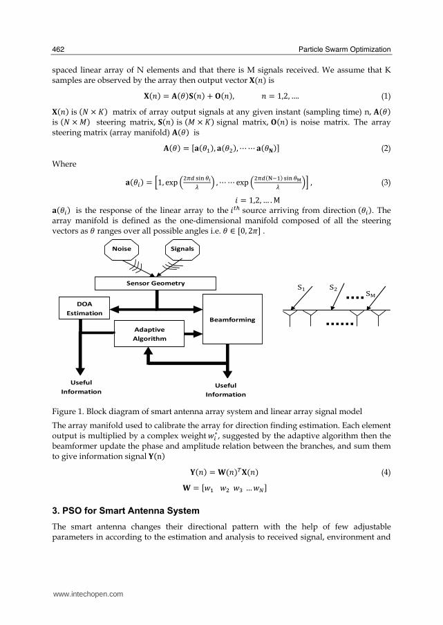
The ability to communicate with people on the move has evolved remarkably since Marconi first demonstrated radio’s ability to provide continuous contact with ships sailing the English Channel in 1897. There onwards, new wireless methods and services have been adopted. Smart antenna system represents one of the valuable parts that support the increasing requirement and needs to higher quality wireless services. Smart antenna systems processes signals arriving from different directions to detect (estimate) desired signal direction of arrival DOA. Biased on the estimated DOA the beamformer optimize antenna elements weights such that the radiation pattern of the antenna array is adjusted to minimize a certain error function or to maximize a certain reward function derived by the adaptive algorithm. Figure 1. Presents block diagram for Smart antenna system. Smart antenna processing core is represented in three areas the adaptive algorithms the DOA estimation algorithm and the beamformer control. One of the simplest geometries for an array is a linear array in which the centers of the antenna elements are aligned along a straight line. For simplicity consider the uniformly

www.intechopen.com

Particle Swarm Optimization

462

spaced linear array of N elements and that there is M signals received. We assume that K samples are observed by the array then output vector 薫岫券岻 is

薫岫券岻噺寓岫肯岻繰岫券岻髪熊岫券岻, 券噺な,に, …. (1) 薫岫券岻 is 岫軽抜計岻 matrix of array output signals at any given instant (sampling time) n, 寓岫肯岻 is 岫軽抜警岻 steering matrix, 繰岫券岻 is 岫警抜計岻 signal matrix, 熊岫券岻 is noise matrix. The array steering matrix (array manifold) 寓岫肯岻 is

寓岫肯岻噺岷軍岫肯怠岻, 軍岫肯態岻, 橋橋軍岫肯窪岻峅 (2)

Where

軍岫肯沈岻噺峙な, exp 岾態訂鳥坦辿樽提日碇峇 , 橋橋 exp 岾態訂鳥岫N貸怠岻坦辿樽提M碇峇峩 , (3) 件噺な,に, … . M 軍岫肯沈岻 is the response of the linear array to the 件痛朕 source arriving from direction 岫肯沈岻. The array manifold is defined as the one-dimensional manifold composed of all the steering vectors as 肯 ranges over all possible angles i.e. 肯樺岷ど, に講峅 .

Figure 1. Block diagram of smart antenna array system and linear array signal model

The array manifold used to calibrate the array for direction finding estimation. Each element output is multiplied by a complex weight 拳沈茅, suggested by the adaptive algorithm then the beamformer update the phase and amplitude relation between the branches, and sum them to give information signal 訓岫n岻

訓岫券岻噺君岫券岻脹薫岫券岻 (4) 君噺岷拳怠拳態拳戴 … 拳朝峅 3. PSO for Smart Antenna System

The smart antenna changes their directional pattern with the help of few adjustable parameters in according to the estimation and analysis to received signal, environment and

Beamforming

Noise Signals

Sensor Geometry

DOA

Estimation

Adaptive

Algorithm

Useful

Information Useful

Information

SM

SにSな

www.intechopen.com


463

pre-known information to improve the performance and capacity of the system. A promising way for the determination of a suitable parameter configuration for the antenna is the application of heuristic optimization procedures. Pattern synthesis problem (beamforming) is continuous varying target real time problem that needs fast optimal solution to adjust array pattern and support for the service required. Also the controlling parameters are limited due to practical design and cost aspects. Consequently Enhancement to PSO algorithm is proposed to support for these two major needs.

3.1 PSO and Dynamic Real Environment Optimization

For real time dynamic environment problem the goal value changes, original PSO algorithm has no method for detecting this change and the particles are still influenced by their memories of the original goal position. If the change in the goal is small, this problem is self-correcting. Subsequent fitness evaluations will result in positions closer to the new goal location replacing earlier position 薫 vectors, and the swarm should follow, and eventually intersect the moving goal. However, if the movement of the goal is more pronounced, it moves too far from the swarm

for subsequent fitness evaluations to return values better than the current personal best 隈沈痛 vector, and the particles do not track the moving goal. A proposed attempt to rectify this

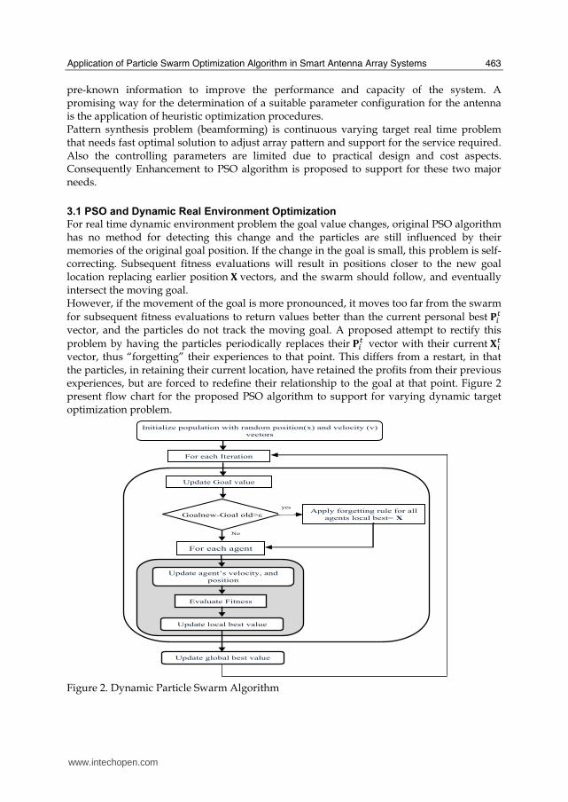
problem by having the particles periodically replaces their 隈沈痛 vector with their current 薫沈痛 vector, thus “forgetting” their experiences to that point. This differs from a restart, in that the particles, in retaining their current location, have retained the profits from their previous experiences, but are forced to redefine their relationship to the goal at that point. Figure 2 present flow chart for the proposed PSO algorithm to support for varying dynamic target optimization problem.

Figure 2. Dynamic Particle Swarm Algorithm

Initialize population with random position(x) and velocity (v)

vectors

For each Iteration

Update Goal value

Update agent’s velocity, and

position

Goalnew-Goal old>ε

For each agent

Evaluate Fitness

Apply forgetting rule for all

agents local best= X

Update global best value

Update local best value

yes

No

www.intechopen.com


464

3.2 PSO and bounded search space

Constraint is usually set to the array parameters these constraints may be spatial, for example, that the interelement spacing be greater than a prescribed value or that the element positions be within specified limits. Other type of design constraint is the excitation where it may require that the elements feed is phase only or amplitude and that the current- taper ratio be less than or equal to a prescribed value. Introducing constraint to the PSO will decrease degree of freedom. Search time will also increase if the concept of accept and after the each particle movement for each iteration according to boundaries. However, if we can convert the problem to an unconstrained one initially through using suitable transformations of the constraint parameter this will eliminate time lost in explore and probability of rejecting the particle movement. Illustration for such solution will be clear in next section while simulation.

4. PSO use for pattern synthesis

This section objects to reformulate and define antenna array adaptive beamforming in term of an optimization problem. Problem Search Space represented by array pattern controlling parameters is identified. Fitness function that measures the deviation of the optimal proposed solution from the target is defined.

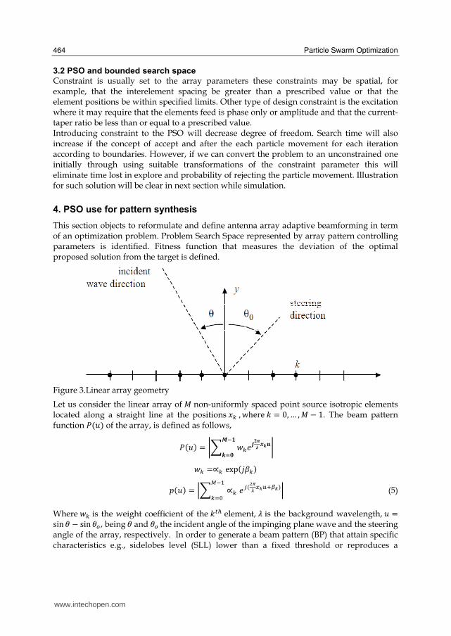
Figure 3.Linear array geometry

Let us consider the linear array of 警 non-uniformly spaced point source isotropic elements located along a straight line at the positions 捲賃 , where 倦噺ど, … , 警伐な. The beam pattern function 鶏岫憲岻 of the array, is defined as follows,

鶏岫憲岻噺嶐布拳賃結斬匝慈似姉暫四捌貸層暫退宋嶐

拳賃噺苅賃 exp岫倹紅賃岻

喧岫憲岻噺鞭布苅賃結珍岫鉄肺敗掴入通袋庭入岻暢貸怠賃退待鞭 (5)

Where 拳賃 is the weight coefficient of the 倦痛朕 element, 膏 is the background wavelength, 憲噺sin 肯伐 sin 肯艇, being 肯 and 肯艇 the incident angle of the impinging plane wave and the steering angle of the array, respectively. In order to generate a beam pattern (BP) that attain specific characteristics e.g., sidelobes level (SLL) lower than a fixed threshold or reproduces a

www.intechopen.com


465

desired shape 鶏鳥喋追勅捗岫憲岻, initially we have to identify the array designing parameters and their

boundaries i.e. The particle search space in PSO algorithm. let vector 賜 be defined as follow, 賜噺岷警, 捲待, … 捲暢貸怠; 拳待 … . 拳暢貸怠; 経峅脹; Where, 警 is number of array elements, 岷捲待, … 捲暢貸怠峅 is array elements spacing vector, 岷拳待 … . 拳暢貸怠峅 is array elements feed vector generally represented as 拳賃噺苅賃結捲喧岫倹紅賃岻, finally 経 is array length. 賜 boundary limits has to be taken in account when solving the problem to facilitate practical and cost design needs. Then a quantized measure for the solution distance from the target required should be defined, this value will be function of the search space parameter vector 賜. Generally for antenna array pattern synthesis most of the well known target consideration is the main beam 血暢喋, total pattern 血喋椎, sidelobe level 血聴挑挑, number, location and width of nulls 血津通鎮, number of array elements 血朝 then we can us define global antenna array fitness function 血, as follows:

血岫賜岻噺怠頂迭捗遁鍋岫賜岻袋頂鉄捗謎遁岫賜岻袋頂典捗縄薙薙岫賜岻袋頂填捗韮祢如岫賜岻袋頂天捗灘岫賜博岻 (6)

Where

血喋牒岫賜岻噺豹岾鶏鳥喋岫憲岻芸⁄ 伐鶏鳥喋追勅捗岫憲岻峇穴憲通樺喋 (7)

血暢喋岫賜岻噺府峭豹岾鶏鳥喋岫憲岻芸⁄ 伐鶏鳥喋追勅捗岫憲岻峇穴憲通樺暢喋嶌陳長沈退怠 (8)

血聴挑挑岫賜岻噺町陳銚掴岶牒匂遁岫通岻岼血剣堅憲鎚痛銚追痛判憲判な (9)

血津通鎮岫賜岻噺府峭豹岾鶏鳥喋岫憲岻芸⁄ 伐鶏鳥喋追勅捗岫憲岻峇穴憲通樺喋朝日嶌津鎮沈退怠

稽軽沈噺憲津通鎮日罰ど.の∆憲津通鎮日 (10)

血朝岫賜岻噺警; (11)

Where 憲鎚痛銚追痛 being a value that allows excluding the main lobe from the calculation of the

SLL. Moreover, 芸 is a normalizing constant, 稽 represents visible region ; while 鶏鳥喋追勅捗岫憲岻

represents the desired BP shape. 警稽 represents the range of values covering the Main beam, mb number of beams in the pattern, 稽軽 corresponds to the nulls locations and 券健 is number of nulls required. Finally, 潔辿 are coefficients that identify each criteria value. It is often necessary to impose a constraint on the interelement spacing to minimize the mutual coupling effects. For and array with an even number of elements the constraint may be expressed as follow

捲怠半鳥態 , 捲沈伐捲沈貸怠半穴件噺に,ぬ, … … 警 (12)

The above constrain can be represented using the following transformation: 捲怠噺鳥態髪岫捲怠́岻態捲態噺岾鳥態髪穴峇髪岫捲怠́岻態髪岫捲態́岻態

www.intechopen.com


466

Generally

岫捲沈岻噺磐件伐なに卑穴髪布岫捲賃́岻態 , 件噺な,に, … . 警沈賃退怠

For odd elements number array

岫捲沈岻噺岫件伐な岻穴髪冨岫捲賃́岻態 , 件噺に, … . 岫警伐な岻/に沈貸怠賃退怠 (13)

Solving using equation 10 allows minimization to be carried out with the new primed variables, and it is readily seen that the constraints are always satisfied. Another type of constraint on spacing’s usually imposed is the one requiring the elements to lie within a specified range mainly required to avoid unacceptable practical array dimensions. Stated mathematically in the following form:

欠沈判捲沈判決沈件噺な,に, … . 警 (14)

the transformation to be used in this case is

捲沈噺欠沈髪岫決沈伐欠沈岻嫌件券態捲徹́ (15)

It is sometimes necessary to constrain the current taper to be within specified limits. That is,

荊沈判荊罰系, 件噺な,に, …. (16)

It is easily verified that the transformation of the form in equation (15) will transform the constrained space into an unconstrained one

荊沈噺荊髪系嫌件券荊徹寐 (17)

Next section will investigate the efficiency of the PSO for solving linear array configuration compared to other algorithms.

4.1 PSO and GA for Pattern Synthesis

To validate the PSO approach, initially we apply PSO, to find the optimized element weight to achieve the Chebyshev pattern for 10 equispaced isotropic elements with λ/2 interelement spacing antenna array of minimum SLL of 26dB, and compare its performance to GA, for solving the same problem. The sample points, are chosen 300 equally distributed points over 憲 on a personal computer with a Pentium IV processor running at 1GHz. The target beam

will be 鶏鳥喋追勅捗

鶏鳥喋追勅捗噺に.ば9 潔剣嫌憲髪に.ね9 潔剣嫌ぬ憲伐ど.9ば潔剣嫌の憲髪な.ぬの潔剣嫌ば憲髪潔剣嫌 9憲

We consider 10 elements symmetric array with amplitude excitation only i.e. 紅沈噺ど then 賜噺釆拳待 … . 拳岾謎鉄峇貸怠挽脹 ; 警噺など

拳賃袋岫暢態⁄ 岻噺拳岫暢態⁄ 岻貸岫賃袋怠岻倦噺ど, … 警に⁄

血喋椎岫賜岻噺に茅廟蕃鶏鳥喋岫憲岻芸伐鶏鳥喋追勅捗岫憲岻否穴憲通樺喋 ; 血剣堅ど判憲判な

www.intechopen.com


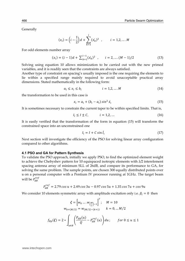
467 血聴挑挑岫賜岻噺態滞陳銚掴祢濡禰尼認禰敦祢敦迭岶牒匂遁岫通岻岼憲鎚痛銚追痛噺ど.にの岫賜岻噺怠捗縄薙薙岫賜博岻袋捗遁鍋岫賜博岻 Figure 4 presents the output pattern explored over the optimization process by one particle until it reaches the optimum solution. Corresponding proposed elements weigh for these local minima is as listed in Table 1.

Iteration No 始宋, 始操始層, 始掻始匝, 始挿始惣, 始掃始想, 始捜 Max. SLL dB

P1 (5) 0.3292 0.5337 0.7030 0.9883 1 -20

P2 (30) 0.3543 0.3243 0.5679 1 0.7044 -15

P3 (78) 0.3521 0.4688 0.7158 0.8378 1 -12

P4 (122) 0.3574 0.4850 0.7055 0.8921 1 -26

Table 1. Optimum proposed weight corresponding to one particle

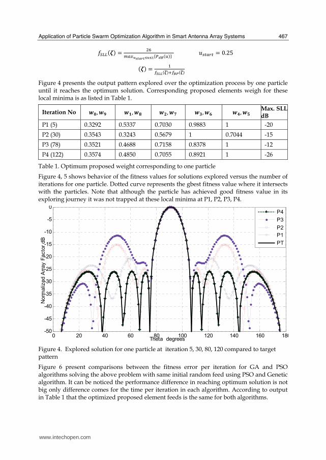
Figure 4, 5 shows behavior of the fitness values for solutions explored versus the number of iterations for one particle. Dotted curve represents the gbest fitness value where it intersects with the particles. Note that although the particle has achieved good fitness value in its exploring journey it was not trapped at these local minima at P1, P2, P3, P4.

Figure 4. Explored solution for one particle at iteration 5, 30, 80, 120 compared to target pattern

Figure 6 present comparisons between the fitness error per iteration for GA and PSO algorithms solving the above problem with same initial random feed using PSO and Genetic algorithm. It can be noticed the performance difference in reaching optimum solution is not big only difference comes for the time per iteration in each algorithm. According to output in Table 1 that the optimized proposed element feeds is the same for both algorithms.

0 20 40 60 80 100 120 140 160 180-50

-45

-40

-35

-30

-25

-20

-15

-10

-5

0

Theta degrees

Norm

aliz

ed A

rray F

acto

r dB

P4

P3

P2

P1

PT

www.intechopen.com


468

Figure 5. Behavior of the fitness function per iteration for one particle, dotted curve represent behavior of gbest fitness value per iteration

Figure 6. Fitness per iteration behavior for PSO algorithm and GA algorithm

Next section will search the capabilities of the PSO for solving array configuration. A simulation for steering single beam, introducing multiple beams in DOA and introducing nulls in the imposed directions by controlling the excitations of the array elements feed or the elements spacing represented in term of λ. also the adaptive ability of PSO for changing the problem target in runtime is presented such feature is to be useful in digital beamforming.

0 10 20 30 40 50 60 70 80 90 100 110 120 130 140 1500

20

40

60

80

100

Iteration Number

% F

itness e

rror

P3 P4

P1

P2

0 10 20 30 40 50 60 70 80 90 100 110 120 130 140 1500

10

20

30

40

50

60

70

Iteration number

% F

itness e

rror

GA

PSO

www.intechopen.com


469

Algorithm/ Normalized weight

始宋, 始操始層, 始掻始匝, 始挿始惣, 始掃始想, 始捜 No. of Iteration

Total time min.

PSO 0.3574 0.4850 0.7055 0.8921 1.000 115 2

GA 0.3563 0.4845 0.7055 0.891 1.000 122 9

Table 2. Optimum proposed weight corresponding to PSO, GA algorithm

4.2 PSO and Pattern Synthesis Phase Control

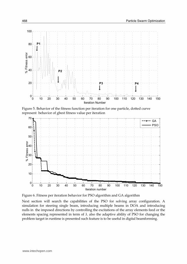
The phase-only null synthesizing is attractive since in a phased array the required controls are available at no extra cost [Steyskal, H.,1986]. This section will illustrate different scenarios for pattern shaping using PSO to search suitable phase feed to fullfill-required pattern. Initially consider it is required to Introduce single null at direction 肯噺50˚ and SLL<30dB with same mainbeam. PSO evaluated element weighting which fulfilled the requirements of the design using fitness function equation 6. Figure 7, shows the output pattern after 200, iteration notice that the SLL criterion is not achieved.

Figure 7. Pattern proposed after 200 iteration for null at 50˚

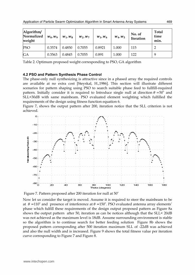
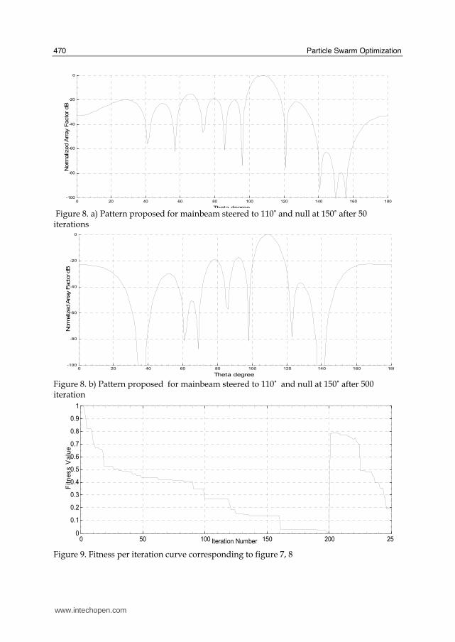
Now let us consider the target is moved. Assume it is required to steer the mainbeam to be at 肯噺110˚ and presence of interference at 肯噺150˚. PSO evaluated antenna array elements’ phase which fulfill these requirements of the design output proposed pattern as Figure 8a shows the output pattern after 50, iteration as can be notices although that the SLL< 20dB was not achieved as the maximum level is 18dB. Assume surrounding environment is stable so the algorithm is to continue search for better feeding solution Figure 8b shows the proposed pattern corresponding after 500 iteration maximum SLL of -22dB was achieved and also the null width and is increased. Figure 9 shows the total fitness value per iteration curve corresponding to Figure 7 and Figure 8.

0 20 40 60 80 100 120 140 160 180-80

-70

-60

-50

-40

-30

-20

-10

0fig

Theta (degree)

Norm

alized Array Factor dB

www.intechopen.com


470

Figure 8. a) Pattern proposed for mainbeam steered to 110˚ and null at 150˚ after 50 iterations

Figure 8. b) Pattern proposed for mainbeam steered to 110˚ and null at 150˚ after 500 iteration

Figure 9. Fitness per iteration curve corresponding to figure 7, 8

0 20 40 60 80 100 120 140 160 180-100

-80

-60

-40

-20

0

Theta degree

Norm

aliz

ed A

rray F

acto

r dB

0 20 40 60 80 100 120 140 160 180-100

-80

-60

-40

-20

0

Theta degree

Norm

aliz

ed A

rray F

acto

r dB

0 50 100 150 200 2500

0.1

0.2

0.3

0.4

0.5

0.6

0.7

0.8

0.9

1

Iteration Number

Fit

ne

ss

Va

lue

www.intechopen.com


471

4.3 PSO and Pattern Synthesis Phase – Position Control

The phase-only synthesis with equal element spacing requires a large number of elements

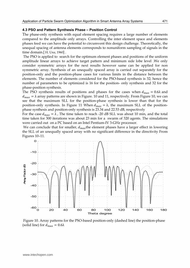
compared to the amplitude only arrays. Controlling the inter element space and elements phases feed we can have the potential to circumvent this design challenge. Theoretically, the unequal spacing of antenna elements corresponds to nonuniform sampling of signals in the time domain.[ H. Unz, 1960] . The PSO is applied to search for the optimum element phases and positions of the uniform amplitude linear arrays to achieve target pattern and minimum side lobe level .We only consider symmetric arrays for the next results however same can be applied for non symmetric array. Synthesis of an unequally spaced array is carried out separately for the position-only and the position-phase cases for various limits in the distance between the elements. The number of elements considered for the PSO-based synthesis is 32; hence the number of parameters to be optimized is 16 for the position- only synthesis and 32 for the phase-position synthesis. The PSO synthesis results of positions and phases for the cases when 穴陳銚掴噺ど.はλ and 穴陳銚掴噺 λ array patterns are shown in Figure. 10 and 11, respectively. From Figure 10, we can see that the maximum SLL for the position-phase synthesis is lower than that for the position-only synthesis. In Figure 11 When 穴陳銚掴噺 λ, the maximum SLL of the position- phase synthesis and position-only synthesis is 23.34 and 22.53 dB, respectively For the case 穴陳銚掴噺 λ , The time taken to reach -20 dB SLL was about 10 min, and the total time taken for 300 iterations was about 23 min for a swarm of 320 agents. The simulations were carried out on a PC based on an Intel Pentium-IV 3-GHz processor. We can conclude that for smaller, 穴陳銚掴the element phases have a larger effect in lowering the SLL of an unequally spaced array with no significant difference in the directivity From Figures 10–11.

Figure 10. Array patterns for the PSO-based position-only (dashed line) the position-phase (solid line) for 穴陳銚掴噺ど.はλ

0 20 40 60 80 100 120 140 160 180-60

-50

-40

-30

-20

-10

0

Theta degree

Array F

actor dB

www.intechopen.com


472

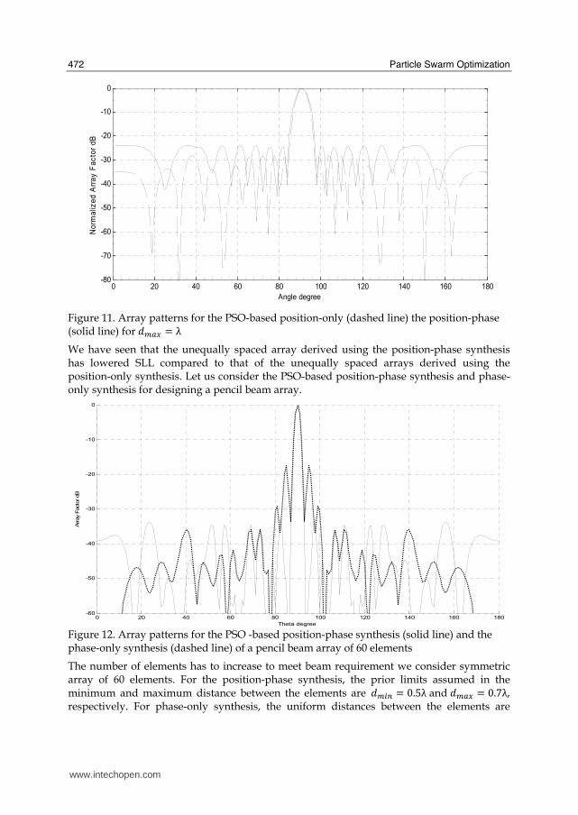
Figure 11. Array patterns for the PSO-based position-only (dashed line) the position-phase (solid line) for 穴陳銚掴噺 λ

We have seen that the unequally spaced array derived using the position-phase synthesis has lowered SLL compared to that of the unequally spaced arrays derived using the position-only synthesis. Let us consider the PSO-based position-phase synthesis and phase-only synthesis for designing a pencil beam array.

Figure 12. Array patterns for the PSO -based position-phase synthesis (solid line) and the phase-only synthesis (dashed line) of a pencil beam array of 60 elements

The number of elements has to increase to meet beam requirement we consider symmetric array of 60 elements. For the position-phase synthesis, the prior limits assumed in the minimum and maximum distance between the elements are 穴陳沈津噺ど.のλ and 穴陳銚掴噺ど.ばλ, respectively. For phase-only synthesis, the uniform distances between the elements are

0 20 40 60 80 100 120 140 160 180-80

-70

-60

-50

-40

-30

-20

-10

0

Angle degree

No

rma

lize

d A

rra

y F

ac

tor

dB

0 20 40 60 80 100 120 140 160 180-60

-50

-40

-30

-20

-10

0

Theta degree

Array F

acto

r dB

www.intechopen.com


473

assumed to be 0.5λ. Figure 12 shows the corresponding array patterns shows the phases and positions derived using the PSO-based phase-only synthesis and position-phase synthesis we can see that for the position-phase synthesis, the SLL is lower compared to that of the phase-only synthesis.

5. PSO Application in Smart Antenna Array Signal Estimation

Conventional adaptive beamforming algorithms are based on a stationary environment. Assume that the desired signal and interferers are not correlated. Using statistical theory, one requires several successive snapshots of the data to form a covariance matrix of the interference with independent identically distributed secondary data[B. D. Van, IEEE 1986]. The snapshots accumulation is quite time consuming. Thus when the environment becomes nonstationary, an inaccurate covariance matrix is derived, which results in that the interference cannot be rejected. Therefore the adaptive processing using a single snapshot [Markus E. Ali ] is more suitable for a dynamic environment. A direct data domain least squares (D3LS) algorithm [T. K. Sarkar, 2000 ] has been developed to analyze the received data using a single snapshot. Although the D3LS algorithm has certain advantages, it has some drawbacks such that the degrees of freedom are limited to nearly half. Furthermore it is shown by simulations that while the jammers can be rejected, the main lobe of the antenna beam pattern is often deviated from the direction of the desired signal and the sidelobe level is relative high.

5.1 Algorithm Formulation

Consider an array composed of 軽 sensors separated by a distance as shown in Figure 1. We assume that narrowband signals consisting of the desired signal plus possibly coherent multipath and jammers with center frequency 血° are impinging on the array from various angles, with the constraint. For sake of simplicity, we assume that the incident fields are coplanar and that they are located in the far field of the array. Each received signal 捲陳岫倦岻 includes additive, zero mean, Gaussian noise. Time is

represented by the 倦痛朕 time sample. Thus, for X岫t岻噺岷捲怠岫倦岻捲態岫倦岻捲N岫倦岻峅T

捲岫倦岻噺岷欠博岫肯怠岻欠博岫肯態岻 …. 欠博岫肯暢岻峅. 琴欽欽欽欣嫌怠岫倦岻嫌態岫倦岻教教嫌暢岫倦岻筋禽禽

禽禁髪券博岫倦岻 (19)

欠博岫肯沈岻 is 警-elements array steering vector for the 肯沈 direction of arrival, 膏 wavelength and 穴 is the elements interspacing distance. 嫌違岫倦岻 is the vector of incident signals at time 倦 and 券博岫倦岻 is noise vector at each array element m, zero mean, variance. Then for 畦違噺岷欠博岫肯怠岻欠博岫肯態岻 …. 欠博岫肯帖岻峅暢抜帖 matrix of steering vectors 欠博岫肯沈岻

X拍噺畦違. 嫌違岫倦岻髪券博岫倦岻 (20)

Thus, each of the D-complex signals arrives at angles 肯沈 and is intercepted by the M antenna elements. It is assumed the number of arriving signals D < M. It is understood that the arriving signals are time varying and thus our calculations are based upon time snapshots of

www.intechopen.com


474

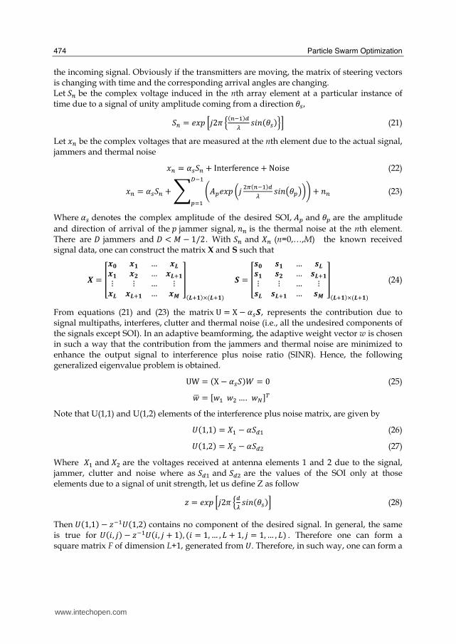
the incoming signal. Obviously if the transmitters are moving, the matrix of steering vectors is changing with time and the corresponding arrival angles are changing. Let 鯨津 be the complex voltage induced in the nth array element at a particular instance of time due to a signal of unity amplitude coming from a direction 肯鎚,

鯨津噺結捲喧峙倹に講峽岫津貸怠岻鳥碇嫌件券岫肯鎚岻峺峩 (21)

Let 捲津 be the complex voltages that are measured at the nth element due to the actual signal, jammers and thermal noise

捲津噺糠鎚鯨津髪 Interference 髪 Noise (22)

捲津噺糠鎚鯨津髪府峭畦椎結捲喧磐倹態訂岫津貸怠岻鳥碇嫌件券盤肯椎匪卑嶌髪券津帖貸怠椎退怠 (23)

Where 糠鎚 denotes the complex amplitude of the desired SOI, 畦椎 and 肯椎 are the amplitude

and direction of arrival of the 喧 jammer signal, 券津 is the thermal noise at the nth element. There are 経 jammers and 経隼警伐な/に. With 鯨津 and 隙津 (n=0,…,M) the known received signal data, one can construct the matrix X and S such that

散噺頒姉宋姉層 … 姉鯖姉層姉匝 … 姉鯖袋層教教 … 教姉鯖姉鯖袋層 … 姉捌番岫鯖袋層岻抜岫鯖袋層岻傘噺頒史宋史層 … 史鯖史層史匝 … 史鯖袋層教教 … 教史鯖史鯖袋層 … 史捌番岫鯖袋層岻抜岫鯖袋層岻 (24)

From equations (21) and (23) the matrix U 噺 X 伐糠鎚傘, represents the contribution due to signal multipaths, interferes, clutter and thermal noise (i.e., all the undesired components of the signals except SOI). In an adaptive beamforming, the adaptive weight vector w is chosen in such a way that the contribution from the jammers and thermal noise are minimized to enhance the output signal to interference plus noise ratio (SINR). Hence, the following generalized eigenvalue problem is obtained.

UW 噺岫X 伐糠鎚鯨岻激噺ど (25) 拳拍噺岷拳怠拳態 …. 拳朝峅脹

Note that U(1,1) and U(1,2) elements of the interference plus noise matrix, are given by

戟岫な,な岻噺隙怠伐糠鯨鳥怠 (26)

戟岫な,に岻噺隙態伐糠鯨鳥態 (27)

Where 隙怠 and 隙態 are the voltages received at antenna elements 1 and 2 due to the signal, jammer, clutter and noise where as 鯨鳥怠 and 鯨鳥態 are the values of the SOI only at those elements due to a signal of unit strength, let us define Z as follow

権噺結捲喧峙倹に講峽鳥碇嫌件券岫肯鎚岻峩 (28)

Then 戟岫な,な岻伐権貸怠戟岫な,に岻 contains no component of the desired signal. In general, the same is true for 戟岫件, 倹岻伐権貸怠戟岫件, 倹髪な岻, 岫件噺な, … , 詣髪な, 倹噺な, … , 詣岻 . Therefore one can form a square matrix F of dimension L+1, generated from 戟. Therefore, in such way, one can form a

www.intechopen.com


475

reduced rank matrix combined with a constraint that the gain of the subarray is C in the direction肯鎚, then one can obtain equation given as follow

頒傑待傑怠 … 傑挑隙待伐傑貸怠隙怠 … … 隙挑伐傑貸怠隙挑袋怠教教教教血戴伐血替傑貸怠 … … 隙暢貸怠伐傑貸怠隙暢番頒激待激怠教激挑番噺頒Cどどど番 (29)

To obtain the desired signal component, equation (5.14) is represented as

岷F峅岷W峅噺岷Y峅 (30)

Using any optimization algorithm to solve equation (30) for, optimum weight vector [W] that provide maximum signal gain through minimizing objective function represented as equation (31)

耕岫W辿岻噺押岷F峅岷W套峅貸Y押押Y押判など貸滞 (31)

Consequently SOI the signal component 糠 may be estimated from

α 噺怠C ∑ 岷W辿X辿峅辿退L辿退待 (32)

The algorithm above is referred to as a “forward method” in the literature [8]. [6],[11]. note we can reformulate the problem using the same data to obtain independent estimate for the solution. This can be achieved by two methods: a. By reversing the data sequence and then complex conjugating each term of that

sequence (Backward method) b. By combining the (forward-backwards method) to double the given data and thereby

increase the number of weights (degrees of freedom) significantly over that of either the forward or backward method alone. The number of degrees of freedom can reach to な髪岫軽伐な岻/な.の.

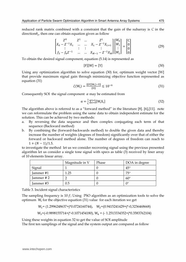
to investigate the method let us we consider recovering signal using the previous presented algorithm let us consider a single tone signal with specs as table (3) received by liner array of 10 elements linear array.

Magnitude in V Phase DOA in degree

Signal 1 0 45°

Jammer #1 1.25 0 75°

Jammer # 2 2 0 60°

Jammer #3 0.5 0 0°

Table 3. Incident signal characteristics

The sampling frequency is 10 血; Using PSO algorithm as an optimization tools to solve the optimum W辿 for the objective equation (31) value for each iteration we get W怠= (1.2996248637+j*0.0724160744), W態=(0.9415241429+j*-0,3236468668) W戴=(-0.9898155714+j*-0.1071454180), W替 = (- 1.2513334352+j*0.3583762104)

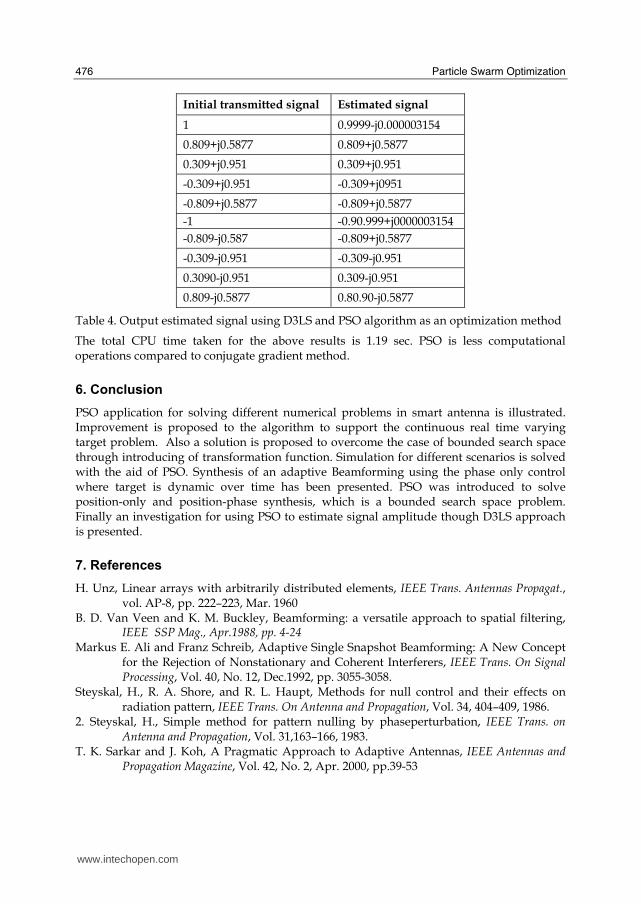
Using these weights in equation 32 to get the value of SOI amplitude The first ten samplings of the signal and the system output are compared as follow

www.intechopen.com


476

Initial transmitted signal Estimated signal

1 0.9999-j0.000003154

0.809+j0.5877 0.809+j0.5877

0.309+j0.951 0.309+j0.951

-0.309+j0.951 -0.309+j0951

-0.809+j0.5877 -0.809+j0.5877

-1 -0.90.999+j0000003154

-0.809-j0.587 -0.809+j0.5877

-0.309-j0.951 -0.309-j0.951

0.3090-j0.951 0.309-j0.951

0.809-j0.5877 0.80.90-j0.5877

Table 4. Output estimated signal using D3LS and PSO algorithm as an optimization method

The total CPU time taken for the above results is 1.19 sec. PSO is less computational operations compared to conjugate gradient method.

6. Conclusion

PSO application for solving different numerical problems in smart antenna is illustrated. Improvement is proposed to the algorithm to support the continuous real time varying target problem. Also a solution is proposed to overcome the case of bounded search space through introducing of transformation function. Simulation for different scenarios is solved with the aid of PSO. Synthesis of an adaptive Beamforming using the phase only control where target is dynamic over time has been presented. PSO was introduced to solve position-only and position-phase synthesis, which is a bounded search space problem. Finally an investigation for using PSO to estimate signal amplitude though D3LS approach is presented.

7. References

H. Unz, Linear arrays with arbitrarily distributed elements, IEEE Trans. Antennas Propagat., vol. AP-8, pp. 222–223, Mar. 1960

B. D. Van Veen and K. M. Buckley, Beamforming: a versatile approach to spatial filtering, IEEE SSP Mag., Apr.1988, pp. 4-24

Markus E. Ali and Franz Schreib, Adaptive Single Snapshot Beamforming: A New Concept for the Rejection of Nonstationary and Coherent Interferers, IEEE Trans. On Signal Processing, Vol. 40, No. 12, Dec.1992, pp. 3055-3058.

Steyskal, H., R. A. Shore, and R. L. Haupt, Methods for null control and their effects on radiation pattern, IEEE Trans. On Antenna and Propagation, Vol. 34, 404–409, 1986.

2. Steyskal, H., Simple method for pattern nulling by phaseperturbation, IEEE Trans. on Antenna and Propagation, Vol. 31,163–166, 1983.

T. K. Sarkar and J. Koh, A Pragmatic Approach to Adaptive Antennas, IEEE Antennas and Propagation Magazine, Vol. 42, No. 2, Apr. 2000, pp.39-53

www.intechopen.com

Particle Swarm OptimizationEdited by Aleksandar Lazinica

ISBN 978-953-7619-48-0Hard cover, 476 pagesPublisher InTechPublished online 01, January, 2009Published in print edition January, 2009

InTech EuropeUniversity Campus STeP Ri Slavka Krautzeka 83/A 51000 Rijeka, Croatia Phone: +385 (51) 770 447 Fax: +385 (51) 686 166www.intechopen.com

InTech ChinaUnit 405, Office Block, Hotel Equatorial Shanghai No.65, Yan An Road (West), Shanghai, 200040, China

Phone: +86-21-62489820 Fax: +86-21-62489821

Particle swarm optimization (PSO) is a population based stochastic optimization technique influenced by thesocial behavior of bird flocking or fish schooling.PSO shares many similarities with evolutionary computationtechniques such as Genetic Algorithms (GA). The system is initialized with a population of random solutionsand searches for optima by updating generations. However, unlike GA, PSO has no evolution operators suchas crossover and mutation. In PSO, the potential solutions, called particles, fly through the problem space byfollowing the current optimum particles. This book represents the contributions of the top researchers in thisfield and will serve as a valuable tool for professionals in this interdisciplinary field.

How to referenceIn order to correctly reference this scholarly work, feel free to copy and paste the following:

May M.M. Wagih and Hassan M. Elkamchouchi (2009). Application of Particle Swarm Optimization Algorithm inSmart Antenna Array Systems, Particle Swarm Optimization, Aleksandar Lazinica (Ed.), ISBN: 978-953-7619-48-0, InTech, Available from:http://www.intechopen.com/books/particle_swarm_optimization/application_of_particle_swarm_optimization_algorithm_in_smart_antenna_array_systems

Documents

Application of Particle Swarm Optimization Algorithm in ...cdn.intechweb.org/pdfs/6279.pdf · Application of Particle Swarm Optimization ... Application of Particle Swarm Optimization