Partial Differential Equations Handout

Peyam Tabrizian

Monday, November 28th, 2011

This handout is meant to give you a couple more examples of all the techniquesdiscussed in chapter 10, to counterbalance all the dry theory and complicated ap-plications in the differential equations book! Enjoy! :)

1 Boundary-Value ProblemsFind the values of λ (eigenvalues) for which the following differential equa-tions has a nonzero solution. Also find the corresponding solutions (eigen-functions)

y′′ + λy = 0

y(0) = 0, y′(π) = 0

The auxiliary polynomial is r2 + λ = 0, which gives r = ±√−λ. Now we

need to proceed with 3 cases:

1

Case 1: λ < 0

Then λ = −ω2, where ω > 0, so: r = ±ω, and the general solution is:

y(t) = Aeωt +Be−ωt

Then y(0) = 0 gives A+B = 0, so B = −A, whence:

y(t) = Aeωt − Ae−ωt

Then:

y′(t) = Aωeωt + Aωe−ωt

Then y′(π) = 0 gives:

Aωeωπ + Aωe−ωπ = 0

Cancelling out A 6= 0 (otherwise B = 0 and Y (y) = 0), we get:

eωπ + e−ωπ = 0

Multiply by eωπ:

e2ωπ + 1 = 0

e2ωπ = −1

However, this doesn’t have a solution because e2ωπ > 0, contradiction.

Case 2: λ = 0. Then we have a double-root r = 0, and:

y(t) = Ae0t +Bte0t = A+Bt

Then y(0) = 0 gives A = 0, and so y(t) = Bt. And y′(π) = 0 gives B = 0,but then y(t) = 0, contradiction.

2

Case 3: λ > 0. Then λ = ω2, where ω > 0.

Then we get r = ±ωi, so:

y(t) = A cos(ωt) +B sin(ωt)

Then: y(0) = 0 gives A = 0, so:

y(t) = B sin(ωt)

Then

y′(t) = ωB cos(ωt)

So y′(π) = 0 gives:

ωB cos(ωπ) = 0

Cancelling out ω andB (because ω > 0, and becauseB 6= 0, otherwiseB = 0and Y (y) = 0), we get:

cos(ωπ) = 0

Which tells you that ωπ = π2+ πM , where M is an integer, so:

ω =M +1

2, (M = 0, 1, 2 · · · )

Answer:This tells you that the eigenvalues are:

λ = ω2 =

(M +

1

2

)2

, (M = 0, 1, 2, · · · )

And the corresponding eigenfunctions are:

y(t) = B sin(ωt) = BM sin

((M +

1

2

)t

)

3

2 Separation of variables

Use the method of separation of variables to ut = uxx to convertthe PDE into two differential equationsSuppose u(x, t) = X(x)T (t)

Then plug this back into ut = uxx:

(X(x)T (t))t = (X(x)T (t))xx

X(x)T ′(t) = X ′′(x)T (t)

Now group the X and the T :

X ′′(x)

X(x)=T ′(t)

T (t)

Now notice that X′′(x)X(x)

only depends on x, but also, by the above equation onlydepends on t, hence it is a constant:

X ′′(x)

X(x)= λ

which gives X ′′(x) = λX(x) .

Moreover: T ′(t)T (t)

= X′′(x)X(x)

= λ, so T ′(t) = λT (t) .

3 Fourier series

3.1 Find the Fourier series of f(x) = x2 on the interval (−3, 3)Here (−T, T ) = (−3, 3), so T = 3

f(x) =∞∑

M=0

AM cos

(πMx

3

)+BM sin

(πMx

3

)Now calculate AM and BM :

4

A0 =

∫ 3

−3 f(x)dx∫ 3

−3 1dx=

∫ 3

−3 x2dx

6=

543

6= 3

AM =

∫ 3

−3 f(x) cos(πMx3

)dx∫ 3

−3 cos2(πMx3

)dx

=

∫ 3

−3 x2 cos

(πMx3

)dx

3=

2

3

∫ 3

0

x2 cos

(πMx

3

)dx

where we used the fact that x2 cos(πMx3

)is even!

Now, to evaluate the integral, use tabular integration:

54/Handouts/Tabular Integration.png

5

2

3

∫ 3

0

x2 cos

(πMx

3

)dx =

2

3

[+x2

(sin(πMx3

)πM3

)−2x

(− cos

(πMx3

)(πM3

)2)+2

(− sin

(πMx3

)(πM3

)3)]3

0

=2

3(−6)

(− cos(πM)(

πM3

)2)

=2

3(6)

(9(−1)M

(πM)2

)=36(−1)M

π2M2

Now for BM : First set B0 = 0 (this is just by definition), and:

BM =

∫ 3

−3 f(x) sin(πMx3

)dx∫ 3

−3 sin2(πMx3

)dx

=

∫ 3

−3 x2 sin

(πMx3

)dx

3= 0

because the numerator is the integral of an odd function over (−3, 3), hence 0.

Putting everything together, we get:

f(x) = 3 +∞∑

M=1

36(−1)M

π2M2cos

(πMx

3

)

6

3.2 To which function does the Fourier series of f converge to?

f(x) =

{x −2 < x < 01 0 ≤ x < 2

Fact: The Fourier series converges to f(x) whenever f is continuous at x,and to f(x−)+f(x+)

2whenever f is discontinuous at x. As for the endpoints, the

Fourier series converges to f(L+)+f(R−)2

, where R is the rightmost endpoint, andL is the leftmost endpoint.

Discontinuity: Here the only discontinuity is at 0, hence at 0, the F.S. con-verges to:

f(0−) + f(0+)

2=

0 + 1

2=

1

2

Endpoints: L = −2, R = 2, so at −2 and 2, the F.S. converges to:

f((−2)+) + f(2−)

2=−2 + 1

2= −1

2

Putting everything together, we find that the F.S. converges to F , where:

F(x) =

−1

2x = −2

x −2 < x < 012

x = 01 0 < x < 2−1

2x = 2

Note: Technically,F is a periodic fuction of period 4, so you’d have to ‘repeat’the graph, just like the picture below!

54/Handouts/Convergence.png

7

8

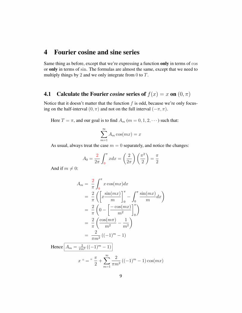
4 Fourier cosine and sine seriesSame thing as before, except that we’re expressing a function only in terms of cosor only in terms of sin. The formulas are almost the same, except that we need tomultiply things by 2 and we only integrate from 0 to T .

4.1 Calculate the Fourier cosine series of f(x) = x on (0, π)

Notice that it doesn’t matter that the function f is odd, because we’re only focus-ing on the half-interval (0, π) and not on the full interval (−π, π).

Here T = π, and our goal is to find Am (m = 0, 1, 2, · · · ) such that:

∞∑m=1

Am cos(mx) = x

As usual, always treat the case m = 0 separately, and notice the changes:

A0 =2

2π

∫ π

0

xdx =

(2

2π

)(π2

2

)=π

2

And if m 6= 0:

Am =2

π

∫ π

0

x cos(mx)dx

=2

π

([xsin(mx)

m

]π0

−∫ π

0

sin(mx)

mdx

)=

2

π

(0−

[− cos(mx)

m2

]π0

)=

2

π

(cos(mπ)

m2− 1

m2

)=

2

πm2((−1)m − 1)

Hence Am = 2πm2 ((−1)m − 1)

x “ = ”π

2+∞∑m=1

2

πm2((−1)m − 1) cos(mx)

9

Now notice that if m is even, then (−1)m − 1 = 0, and hence Am = 0. And ifm is odd,then (−1)m − 1 = −2, so Am = −4

πm2

Therefore:

x“ = ”π

2+

∞∑m=1,modd

−4πm2

cos(mx)

x“ = ”π

2− 4

π

∞∑k=1

−4π(2k − 1)2

cos((2k − 1)x)

This is because every odd numberm ≥ 1 can be written asm = 2k−1, wherek = 1, 2, · · · .

4.2 Calculate the Fourier sine series of f(x) = x on (0, π)

Here T = π, and our goal is to find Bm (m = 0, 1, 2, · · · ) such that:

∞∑m=1

Bm sin(mx) = x

As usual, always treat the case m = 0 separately, namely set B0 = 0.

And if m 6= 0:

Bm =2

π

∫ π

0

x sin(mx)dx

=2

π

([−xcos(mx)

m

]π0

−∫ π

0

− cos(mx)

mdx

)=

2

π

(−π cos(mπ) +

[sin(mx)

m2

]π0

)=

2

π(−π(−1)m)

= 2(−1)m+1

Hence Bm = 2(−1)m+1 , and:

10

x“ = ”∞∑m=1

2(−1)m+1 sin(mx)

11

5 The Heat equationProblem: Solve the following heat equation:

∂u

∂t=

∂2u

∂x20 < x < 1, t > 0

u(0, t) = u(1, t) = 0 t > 0

u(x, 0) = x 0 < x < 1

(5.1)

Step 1: Separation of variablesSuppose:

u(x, t) = X(x)T (t) (5.2)

Plug (5.2) into the differential equation (5.1), and you get:

(X(x)T (t))t =(X(x)T (t))xxX(x)T ′(t) =X ′′(x)T (t)

Rearrange and get:

X ′′(x)

X(x)=T ′(t)

T (t)(5.3)

Now X′′(x)X(x)

only depends on x, but by (5.3) only depends on t, hence it isconstant:

X ′′(x)

X(x)=λ

X ′′(x) =λX(x)

(5.4)

Also, we get:

T ′(t)

T (t)=λ

T ′(t) =λT (t)

(5.5)

12

but we’ll only deal with that later (Step 4)

Step 2:Consider (5.4):

X ′′(x) = λX(x)

Note: Always start with X(x), do NOT touch T (t) until right at the end!

Now use the boundary conditions in (5.1):

u(0, t) = X(0)T (t) = 0⇒ X(0)T (t) = 0⇒ X(0) = 0

u(1, t) = X(1)T (t) = 0⇒ X(1)T (t) = 0⇒ X(1) = 0

Hence we get: X ′′(x) =λX(x)

X(0) =0

X(1) =0

(5.6)

Step 3: Eigenvalues/EigenfunctionsThe auxiliary polynomial of (5.6) is p(λ) = r2 − λ

Now we need to consider 3 cases:

Case 1: λ > 0, then λ = ω2, where ω > 0

Then:

r2 − λ = 0⇒ r2 − ω2 = 0⇒ r = ±ω

Therefore:

X(x) = Aeωx +Be−ωx

13

Now use X(0) = 0 and X(1) = 0:

X(0) = 0⇒ A+B = 0⇒ B = −A⇒ X(x) = Aeωx − Ae−ωx

X(1) = 0⇒ Aeω−Ae−ω = 0⇒ Aeω = Ae−ω ⇒ eω = e−ω ⇒ ω = −ω ⇒ ω = 0

But this is a contradiction, as we want ω > 0.

Case 2: λ = 0, then r = 0, and:

X(x) = Ae0x +Bxe0x = A+Bx

And:

X(0) = 0⇒ A = 0⇒ X(x) = Bx

X(1) = 0⇒ B = 0⇒ X(x) = 0

Again, a contradiction (we want X��≡ 0, because otherwise u(x, t) ≡ 0)

Case 3: λ < 0, then λ = −ω2, and:

r2 − λ = 0⇒ r2 + ω2 = 0⇒ r = ±ωiWhich gives:

X(x) = A cos(ωx) +B sin(ωx)

Again, using X(0) = 0, X(1) = 0, we get:

X(0) = 0⇒ A = 0⇒ X(x) = B sin(ωx)

X(1) = 0⇒ B sin(ω) = 0⇒ sin(ω) = 0⇒ ω = πm, (m = 1, 2, · · · )

This tells us that:

Eigenvalues:λ = −ω2 = −(πm)2 (m = 1, 2, · · · )Eigenfunctions:X(x) = sin(ωx) = sin(πmx)

(5.7)

14

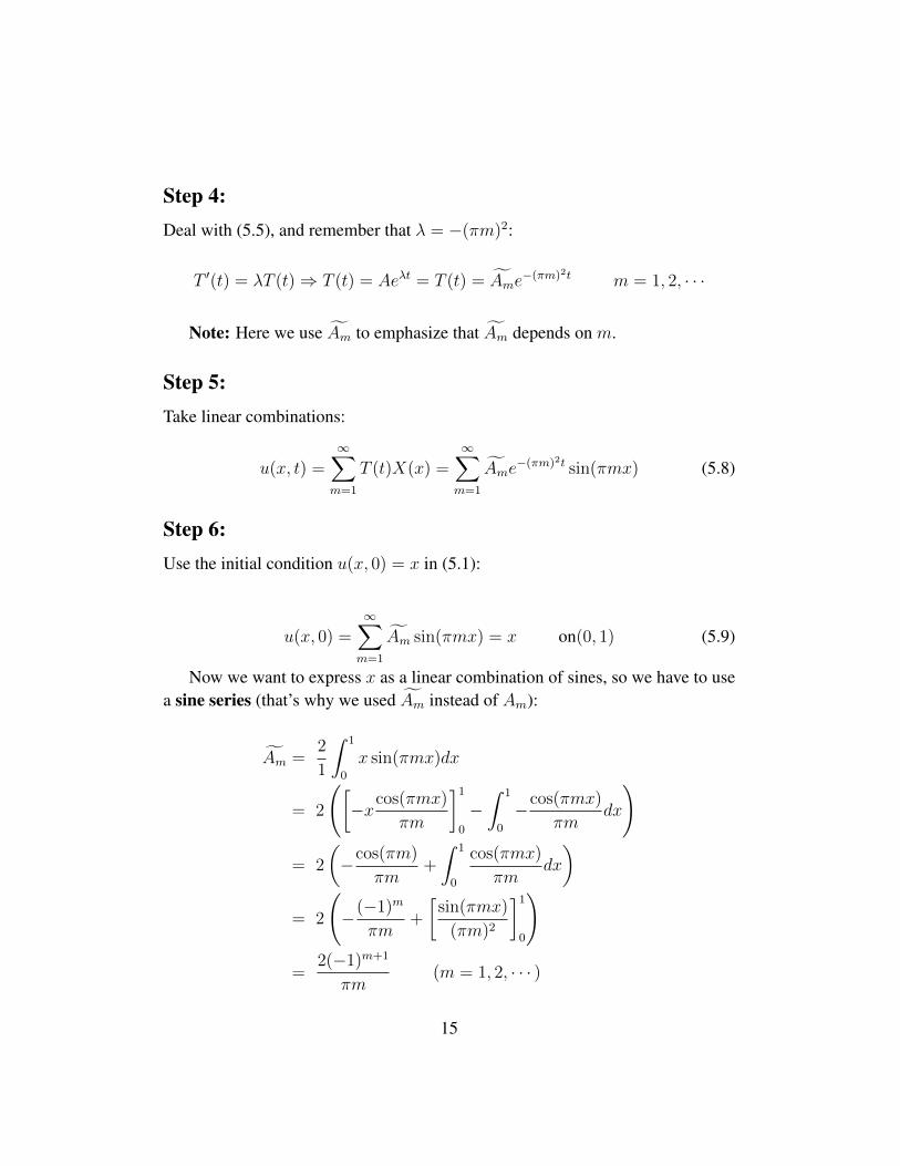
Step 4:Deal with (5.5), and remember that λ = −(πm)2:

T ′(t) = λT (t)⇒ T (t) = Aeλt = T (t) = Ame−(πm)2t m = 1, 2, · · ·

Note: Here we use Am to emphasize that Am depends on m.

Step 5:Take linear combinations:

u(x, t) =∞∑m=1

T (t)X(x) =∞∑m=1

Ame−(πm)2t sin(πmx) (5.8)

Step 6:Use the initial condition u(x, 0) = x in (5.1):

u(x, 0) =∞∑m=1

Am sin(πmx) = x on(0, 1) (5.9)

Now we want to express x as a linear combination of sines, so we have to usea sine series (that’s why we used Am instead of Am):

Am =2

1

∫ 1

0

x sin(πmx)dx

= 2

([−xcos(πmx)

πm

]10

−∫ 1

0

−cos(πmx)

πmdx

)

= 2

(−cos(πm)

πm+

∫ 1

0

cos(πmx)

πmdx

)= 2

(−(−1)m

πm+

[sin(πmx)

(πm)2

]10

)

=2(−1)m+1

πm(m = 1, 2, · · · )

15

Step 7:Conclude using (5.10)

u(x, t) =∞∑m=1

2(−1)m+1

πme−(πm)2t sin(πmx) (5.10)

16

6 The Wave equationProblem: Solve the following wave equation:

∂2u

∂t2=

∂2u

∂x20 < x < π, t > 0

u(0, t) = u(π, t) = 0 t > 0

u(x, 0) = sin(4x) + 7 sin(5x) 0 < x < π

∂u

∂t(x, 0) = 2 sin(2x) + sin(3x) 0 < x < π

(6.1)

Step 1: Separation of variablesSuppose:

u(x, t) = X(x)T (t) (6.2)

Plug (6.2) into the differential equation (6.1), and you get:

(X(x)T (t))tt =(X(x)T (t))xxX(x)T ′′(t) =X ′′(x)T (t)

Rearrange and get:

X ′′(x)

X(x)=T ′′(t)

T (t)(6.3)

Now X′′(x)X(x)

only depends on x, but by (6.3) only depends on t, hence it isconstant:

X ′′(x)

X(x)=λ

X ′′(x) =λX(x)

(6.4)

Also, we get:

17

T ′′(t)

T (t)=λ

T ′′(t) =λT (t)

(6.5)

but we’ll only deal with that later (Step 4)

Step 2:Consider (6.4):

X ′′(x) = λX(x)

Note: Always start with X(x), do NOT touch T (t) until right at the end!

Now use the boundary conditions in (6.1):

u(0, t) = X(0)T (t) = 0⇒ X(0)T (t) = 0⇒ X(0) = 0

u(π, t) = X(π)T (t) = 0⇒ X(π)T (t) = 0⇒ X(π) = 0

Hence we get: X ′′(x) =λX(x)

X(0) =0

X(π) =0

(6.6)

Step 3: Eigenvalues/EigenfunctionsThe auxiliary polynomial of (6.6) is p(λ) = r2 − λ

Now we need to consider 3 cases:

Case 1: λ > 0, then λ = ω2, where ω > 0

Then:

18

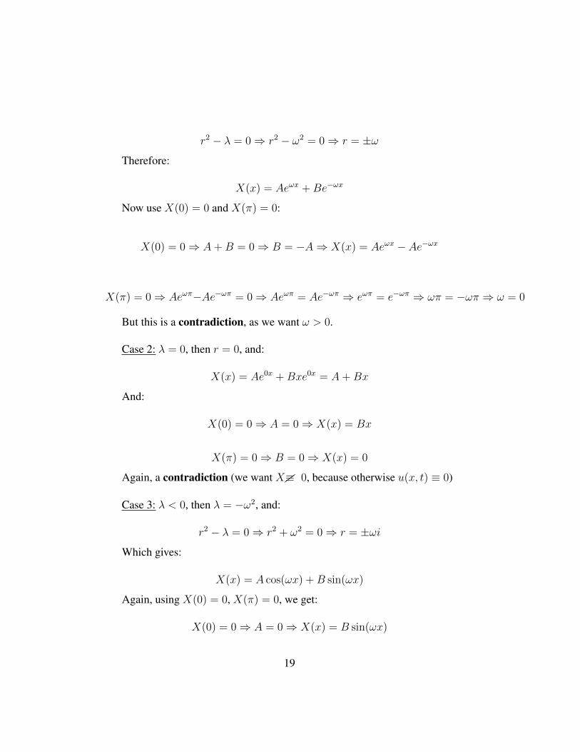
r2 − λ = 0⇒ r2 − ω2 = 0⇒ r = ±ω

Therefore:

X(x) = Aeωx +Be−ωx

Now use X(0) = 0 and X(π) = 0:

X(0) = 0⇒ A+B = 0⇒ B = −A⇒ X(x) = Aeωx − Ae−ωx

X(π) = 0⇒ Aeωπ−Ae−ωπ = 0⇒ Aeωπ = Ae−ωπ ⇒ eωπ = e−ωπ ⇒ ωπ = −ωπ ⇒ ω = 0

But this is a contradiction, as we want ω > 0.

Case 2: λ = 0, then r = 0, and:

X(x) = Ae0x +Bxe0x = A+Bx

And:

X(0) = 0⇒ A = 0⇒ X(x) = Bx

X(π) = 0⇒ B = 0⇒ X(x) = 0

Again, a contradiction (we want X��≡ 0, because otherwise u(x, t) ≡ 0)

Case 3: λ < 0, then λ = −ω2, and:

r2 − λ = 0⇒ r2 + ω2 = 0⇒ r = ±ωi

Which gives:

X(x) = A cos(ωx) +B sin(ωx)

Again, using X(0) = 0, X(π) = 0, we get:

X(0) = 0⇒ A = 0⇒ X(x) = B sin(ωx)

19

X(π) = 0⇒ B sin(ωπ) = 0⇒ sin(ωπ) = 0⇒ ω = m, (m = 1, 2, · · · )

This tells us that:

Eigenvalues:λ = −ω2 = −m2 (m = 1, 2, · · · )Eigenfunctions:X(x) = sin(ωx) = sin(mx)

(6.7)

Step 4:Deal with (6.5), and remember that λ = −m2:

T ′′(t) = λT (t)

Aux: r2 = −m2 ⇒ r = ±mi (m = 1, 2, · · · )

T (t) = Am cos(mt) + Bm sin(mt)

Step 5:Take linear combinations:

u(x, t) =∞∑m=1

T (t)X(x) =∞∑m=1

(Am cos(mt) + Bm sin(mt)

)sin(mx) (6.8)

Step 6:Use the initial condition u(x, 0) = sin(4x) + 7 sin(5x) in (6.1):

Plug in t = 0 in (6.8), and you get:

u(x, 0) =∞∑m=1

Am sin(mx) = sin(4x) + 7 sin(5x) on(0, π) (6.9)

20

Note: At this point you would usually have to find the sine series of a function(see section 4). But here we’re very lucky because we’re already given a linearcombination of sines!

Equating coefficients, you get:

A4 = 1 (coefficient of sin(4x))

A5 = 7 (coefficient of sin(5x))

Am = 0 (for all other m)

Step 7:Use the initial condition: ∂u

∂t(x, 0) = 2 sin(2x) + sin(3x) in (6.1)

First differentiate (6.8) with respect to t:

∂u

∂t(x, t) =

∞∑m=1

(−mAm sin(mt) +mBm cos(mt)

)sin(mx) (6.10)

Now plug in t = 0 in (6.10):

∂u

∂t(x, 0) =

∞∑m=1

mBm sin(mx) = 2 sin(2x) + sin(3x) (6.11)

Again, usually you’d have to calculate Fourier sine series, but again we’relucky because the right-hand-side is already a linear combination of sines!

Equating coefficients, you get:

2B2 = 2 (coefficient of sin(2x))

3B3 = 1 (coefficient of sin(3x))

Bm = 0 (for all other m)

That is:

21

B2 = 1 (coefficient of sin(2x))

B3 =1

3(coefficient of sin(3x))

Bm = 0 (for all other m)

Step 8:Conclude using (6.8) and the coefficients Am and Bm you found:

u(x, t) =∞∑m=1

(Am cos(mt) + Bm sin(mt)

)sin(mx) (6.12)

where:

A4 = 1

A5 = 7

Am = 0 (for all other m)

and

B2 = 1

B3 =1

3

Bm = 0 (for all other m)

Note: In this special case, you can write u(x, t) in the following nice form:

u(x, t) = sin(2t) sin(2x)+1

3sin(3t) sin(3x)+cos(4t) sin(4x)+7 cos(5t) sin(5x)

(6.13)But in general, you’d have to leave your answer in the form of (6.8)

22

7 Laplace’s equationProblem: Solve the following Laplace equation:

∂2u

∂x2+∂2u

∂y2= 0 0 < x < 1, 0 < y < 1

u(0, y) = u(1, y) =0 0 ≤ y ≤ 1

u(x, 0) = 6 sin(5πx) 0 ≤ x ≤ 1

u(x, 1) = 0 0 ≤ x ≤ 1

(7.1)

Step 1: Separation of variablesSuppose:

u(x, y) = X(x)Y (y) (7.2)

Plug (7.2) into the differential equation (7.1), and you get:

(X(x)Y (y))xx + (X(x)Y (y))yy =0

X ′′(x)Y (y) +X(x)Y ′′(y) =0

X ′′(x)Y (y) =−X(x)Y ′′(y)

Rearrange and get:

X ′′(x)

X(x)=−Y ′′(y)Y (y)

(7.3)

Now X′′(x)X(x)

only depends on x, but by (7.3) only depends on y, hence it isconstant:

X ′′(x)

X(x)=λ

X ′′(x) =λX(x)

(7.4)

Also, we get:

23

−Y ′′(y)Y (y)

=λ

Y ′′(y) =− λY (y)

(7.5)

but we’ll only deal with that later (Step 4)

Note: Careful about the − sign!!!

Step 2:Consider (7.4):

X ′′(x) = λX(x)

Note: Always start with X(x), do NOT touch Y (y) until right at the end!

Now use the boundary conditions in (7.1):

u(0, y) = X(0)Y (y) = 0⇒ X(0)Y (y) = 0⇒ X(0) = 0

u(1, y) = X(1)Y (1) = 0⇒ X(1)Y (y) = 0⇒ X(1) = 0

Hence we get: X ′′(x) =λX(x)

X(0) =0

X(1) =0

(7.6)

Step 3: Eigenvalues/EigenfunctionsThe auxiliary polynomial of (7.6) is p(λ) = r2 − λ

Now we need to consider 3 cases:

Case 1: λ > 0, then λ = ω2, where ω > 0

24

Then:

r2 − λ = 0⇒ r2 − ω2 = 0⇒ r = ±ω

Therefore:

X(x) = Aeωx +Be−ωx

Now use X(0) = 0 and X(1) = 0:

X(0) = 0⇒ A+B = 0⇒ B = −A⇒ X(x) = Aeωx − Ae−ωx

X(1) = 0⇒ Aeω−Ae−ω = 0⇒ Aeω = Ae−ω ⇒ eω = e−ω ⇒ ω = −ω ⇒ ω = 0

But this is a contradiction, as we want ω > 0.

Case 2: λ = 0, then r = 0, and:

X(x) = Ae0x +Bxe0x = A+Bx

And:

X(0) = 0⇒ A = 0⇒ X(x) = Bx

X(1) = 0⇒ B = 0⇒ X(x) = 0

Again, a contradiction (we want X��≡ 0, because otherwise u(x, y) ≡ 0)

Case 3: λ < 0, then λ = −ω2, and:

r2 − λ = 0⇒ r2 + ω2 = 0⇒ r = ±ωi

Which gives:

X(x) = A cos(ωx) +B sin(ωx)

Again, using X(0) = 0, X(1) = 0, we get:

X(0) = 0⇒ A = 0⇒ X(x) = B sin(ωx)

25

X(1) = 0⇒ B sin(ω) = 0⇒ sin(ω) = 0⇒ ω = πm, (m = 1, 2, · · · )

This tells us that:

Eigenvalues:λ = −ω2 = −(πm)2 (m = 1, 2, · · · )Eigenfunctions:X(x) = sin(ωx) = sin(πmx)

(7.7)

Step 4:Deal with (7.5), and remember that λ = −(πm)2:

Y ′′(y) = −λY (y)

Aux: r2 = (πm)2 ⇒ r = ±πm (m = 1, 2, · · · )

Y (y) = Ameπmy + Bme

−πmy (7.8)

IMPORTANT REMARK: If you leave your answer like that, your algebrabecomes messy! Instead, use the following nice formulas:

ew + e−w

2= cosh(w)

ew − e−w

2= sinh(w)

And you get:

Y (y) = Am cosh(πmy) + Bm sinh(πmy) (7.9)

Note: The constants Am and Bm are different in (7.8) and (7.9), but it doesn’tmatter because they are only (general) constants!

Step 5:Take linear combinations:

26

u(x, t) =∞∑m=1

Y (y)X(x) =∞∑m=1

(Am cosh(πmy) + Bm sinh(πmy)

)sin(πmx)

(7.10)

Step 6:Use the initial condition u(x, 0) = 6 sin(5πx) in (7.1):

Plug in y = 0 in (7.10), and using cosh(0) = 1, sinh(0) = 0, you get:

u(x, 0) =∞∑m=1

Am sin(πmx) = 6 sin(5πx) on(0, 1) (7.11)

Note: At this point you would usually have to find the sine series of a function(see the heat equation example). But here again we’re very lucky because we’realready given a linear combination of sines!

Equating coefficients (notice this is why we used cosh and sinh instead ofexponential functions), you get:

A5 = 6 (coefficient of sin(5πx))

Am = 0 (for all other m)(7.12)

Step 7:Use the initial condition: u(x, 1) = 0 in (7.1)

Plug in y = 1 in (7.8), and you get:

u(x, 1) =∞∑m=1

(Am cosh(πm) + Bm sinh(πm)

)sin(πmx) = 0 on(0, 1)

(7.13)Again, usually you’d have to use a Fourier sine series, but again you’re lucky

because the function is 0, so if you equate the coefficients, you get:

cosh(πm)Am + sinh(πm)Bm = 0 (m = 1, 2, · · · ) (7.14)

27

But now combining (7.10) and (7.18), we get:

For m 6= 5 Am = 0, so:

sinh(πm)Bm = 0 (7.15)

which gives you Bm = 0 for m 6= 5.

For m = 5:

cosh(5π)6 + sinh(5π)B5 = 0 (7.16)

which gives you:

B5 = −6 cosh(5π)

sinh(5π)= −6 coth(5π)

Step 8:Conclude using (7.10) and the coefficients Am and Bm you found:

u(x, y) =∞∑m=1

Y (y)X(x) =∞∑m=1

(Am cosh(πmy) + Bm sinh(πmy)

)sin(πmx)

(7.17)

where: Am = Bm = 0 if m 6= 5, and A5 = 6, B5 = −6 coth(5π) .

Note: In this special case, you can write u(x, t) in the following nice form:

u(x, y) = (6 cosh(5πy)− 6 coth(5π) sinh(5πy)) sin(πmx) (7.18)

But in general, you’d have to leave your answer in the general form (7.10).

28