Embed Size (px)
Citation preview
Part 4: MEASURING CONTAMINANT CONCENTRATIONS IN SOIL
The Soil Screening Guidance includes a sampling strategy for implementing the soil screening process.Section 4.1 presents the sampling approach for surface soils. This approach provides a simpledecision rule based on comparing the maximum contaminant concentrations of composite sampleswith surface soil screening levels (the Max test) to determine whether further investigation is neededfor a particular exposure area (EA). In addition, this section presents a more complex strategy (theChen test) that allows the user to design a site-specific quantitative sampling strategy by varyingdecision error limits and soil contaminant variability to optimize the number of samples andcomposites. Section 4.2 provides a subsurface soil sampling strategy for developing SSLs and applyingthe screening procedure for the volatilization and migration to ground water exposure pathways.
Section 4.3 describes the technical details behind the development of the SSL sampling strategy,including analyses and response to public and peer-review comments received on the December 1994draft guidance.
The sampling strategy for the soil screening process is designed to achieve the following objectives:
• Estimate mean concentrations of contaminants of concern forcomparison with SSLs
• Fill in the data gaps in the conceptual site model necessary to developSSLs.
The soils of interest for the first objective differ according to the exposure pathway being addressed.For the direct ingestion, dermal, and fugitive dust pathways, EPA is concerned about surface soils.The sampling goal is to determine average contaminant concentrations of surface soils in exposureareas of concern. For inhalation of volatiles, migration to ground water and, in some cases, plantuptake, subsurface soils are the primary concern. For these pathways, the average contaminantconcentration through each source is the parameter of interest.
The second objective (filling in the data gaps) applies primarily to the inhalation and migration toground water pathways. For these pathways, the source area and depth as well as average soilproperties within the source are needed to calculate the pathway-specific SSLs. Therefore, thesampling strategy needs to address collection of these site-specific data.
Because of the difference in objectives, the sampling strategies for the ingestion pathway and for theinhalation and migration to ground water pathways are addressed separately. If both surface andsubsurface soils are a concern, then surface soils should be sampled first because the results of surfacesoil analyses may help delineate source areas to target for subsurface sampling.
At some sites, a third sampling objective may be appropriate. As discussed in the Soil ScreeningGuidance, SSLs may not be useful at sites where background contaminant levels are above the SSLs.Where sampling information suggests that background contaminant concentrations may be aconcern, background sampling may be necessary. Methods for Evaluating the Attainment of CleanupStandards - Volume 3: Reference-Based Standards for Soil and Solid Media (U.S. EPA, 1994e)provides further information on sampling soils to determine background conditions at a site.
81
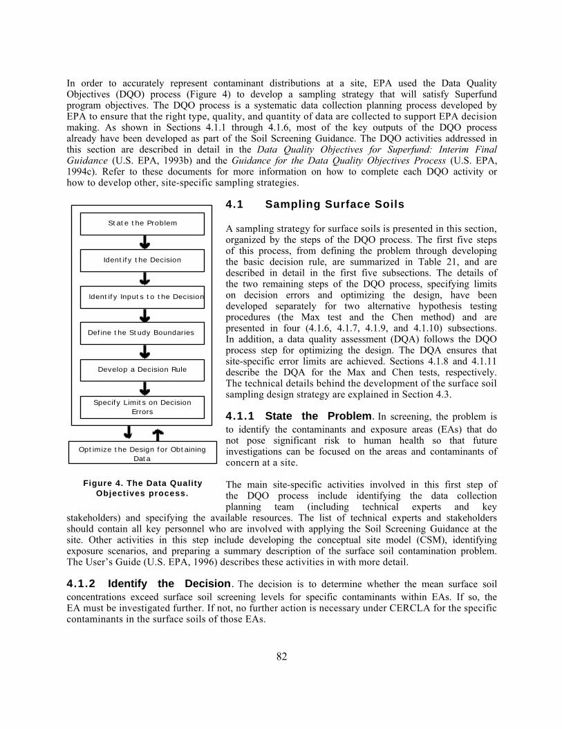
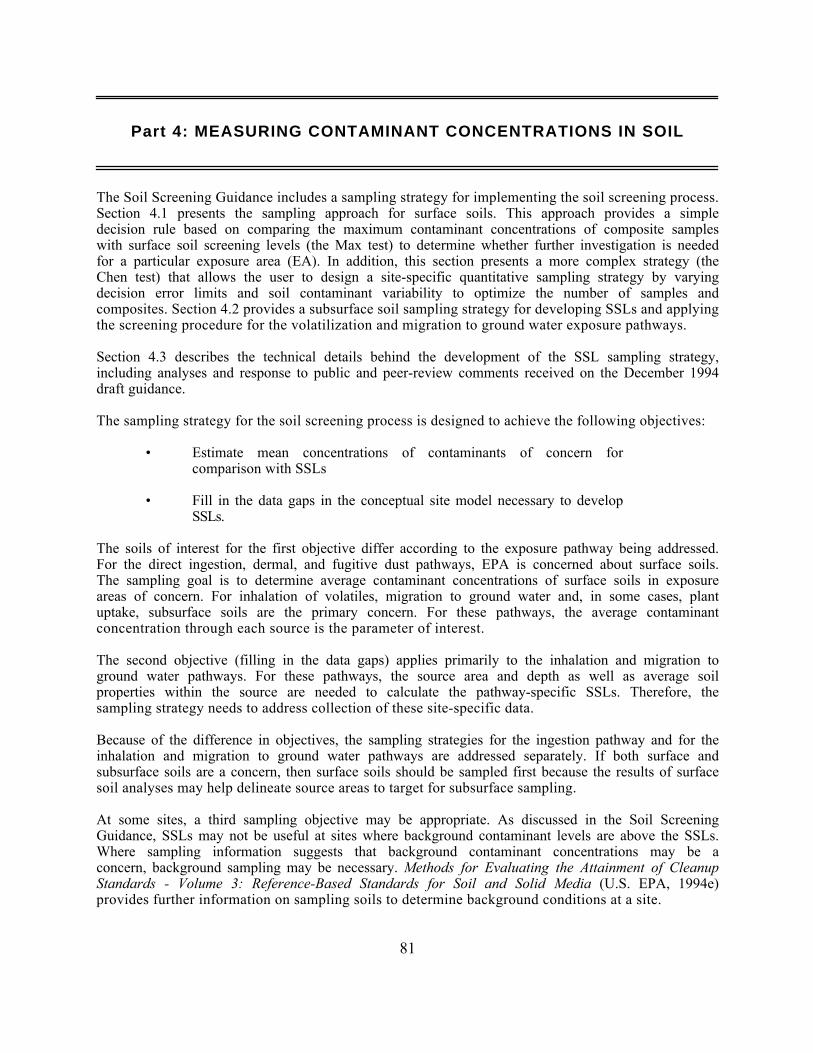
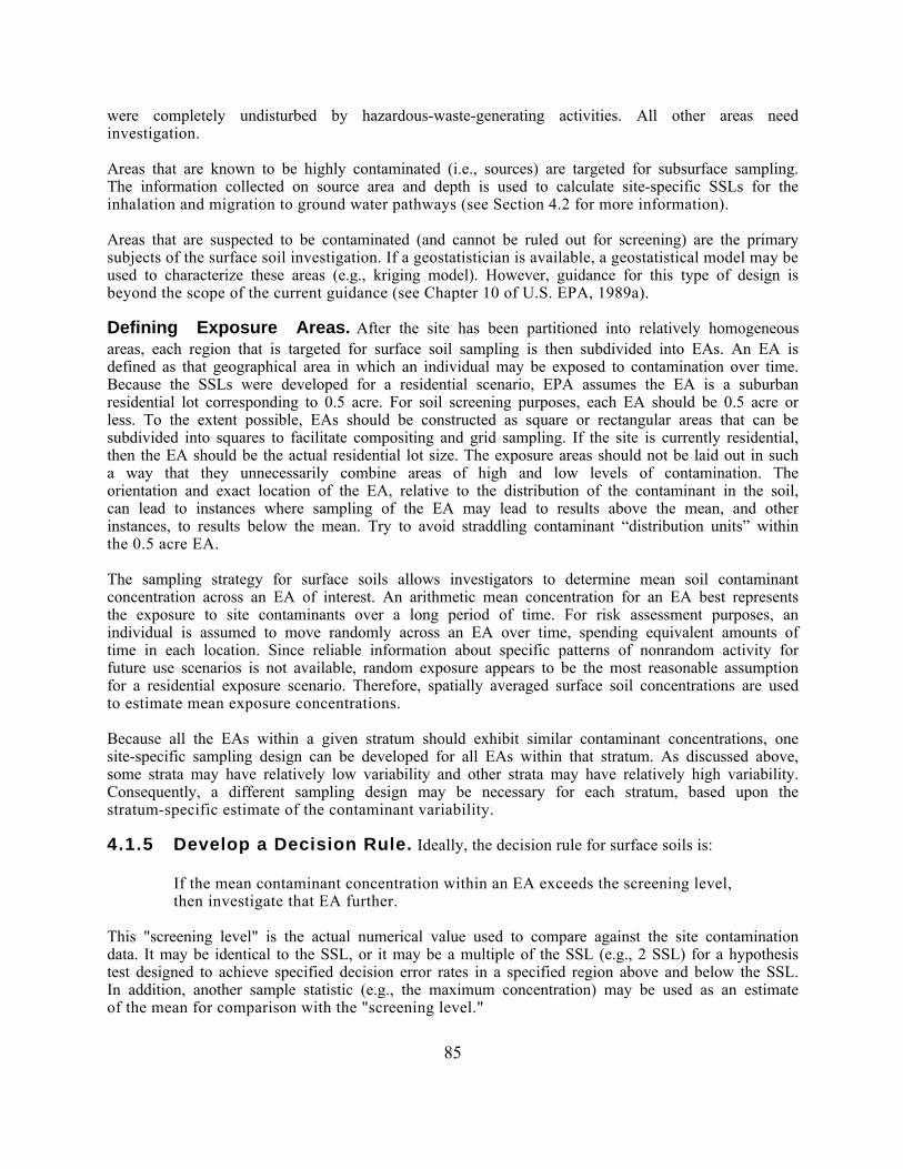
In order to accurately represent contaminant distributions at a site, EPA used the Data QualityObjectives (DQO) process (Figure 4) to develop a sampling strategy that will satisfy Superfundprogram objectives. The DQO process is a systematic data collection planning process developed byEPA to ensure that the right type, quality, and quantity of data are collected to support EPA decisionmaking. As shown in Sections 4.1.1 through 4.1.6, most of the key outputs of the DQO processalready have been developed as part of the Soil Screening Guidance. The DQO activities addressed inthis section are described in detail in the Data Quality Objectives for Superfund: Interim FinalGuidance (U.S. EPA, 1993b) and the Guidance for the Data Quality Objectives Process (U.S. EPA,1994c). Refer to these documents for more information on how to complete each DQO activity orhow to develop other, site-specific sampling strategies.
State the Problem
Identify the Decision
Identify Inputs to the Decision
Define the Study Boundaries
Develop a Decision Rule
Specify Limits on DecisionErrors
Optimize the Design for ObtainingData
Figure 4. The Data QualityObjectives process.
4.1 Sampling Surface Soils
A sampling strategy for surface soils is presented in this section,organized by the steps of the DQO process. The first five stepsof this process, from defining the problem through developingthe basic decision rule, are summarized in Table 21, and aredescribed in detail in the first five subsections. The details ofthe two remaining steps of the DQO process, specifying limitson decision errors and optimizing the design, have beendeveloped separately for two alternative hypothesis testingprocedures (the Max test and the Chen method) and arepresented in four (4.1.6, 4.1.7, 4.1.9, and 4.1.10) subsections.In addition, a data quality assessment (DQA) follows the DQOprocess step for optimizing the design. The DQA ensures thatsite-specific error limits are achieved. Sections 4.1.8 and 4.1.11describe the DQA for the Max and Chen tests, respectively.The technical details behind the development of the surface soilsampling design strategy are explained in Section 4.3.
4.1.1 State the Problem. In screening, the problem isto identify the contaminants and exposure areas (EAs) that donot pose significant risk to human health so that futureinvestigations can be focused on the areas and contaminants ofconcern at a site.
The main site-specific activities involved in this first step ofthe DQO process include identifying the data collectionplanning team (including technical experts and key
stakeholders) and specifying the available resources. The list of technical experts and stakeholdersshould contain all key personnel who are involved with applying the Soil Screening Guidance at thesite. Other activities in this step include developing the conceptual site model (CSM), identifyingexposure scenarios, and preparing a summary description of the surface soil contamination problem.The User’s Guide (U.S. EPA, 1996) describes these activities in with more detail.
4.1.2 Identify the Decision. The decision is to determine whether the mean surface soilconcentrations exceed surface soil screening levels for specific contaminants within EAs. If so, theEA must be investigated further. If not, no further action is necessary under CERCLA for the specificcontaminants in the surface soils of those EAs.
82
Table 21. Sampling Soil Screening DQOs for Surface Soils
DQO Process Steps Soil Screening Inputs/Outputs
State the Problem
Identify scoping team Site manager and technical experts (e.g., toxicologists, risk assessors,statisticians, soil scientists)
Develop conceptual site model (CSM) CSM development (described in Step 1 of the User’s Guide, U.S. EPA, 1996)
Define exposure scenarios Direct ingestion and inhalation of fugitive particulates in a residential setting;dermal contact and plant uptake for certain contaminants
Specify available resources Sampling and analysis budget, scheduling constraints, and availablepersonnel
Write brief summary of contaminationproblem
Summary of the surface soil contamination problem to be investigated at thesite
Identify the Decision
Identify decision Do mean soil concentrations for particular contaminants (e.g., contaminants ofpotential concern) exceed appropriate screening levels?
Identify alternative actions Eliminate area from further study under CERCLAorPlan and conduct further investigation
Identify Inputs to the Decision
Identify inputs Ingestion and particulate inhalation SSLs for specified contaminantsMeasurements of surface soil contaminant concentration
Define basis for screening Soil Screening Guidance
Identify analytical methods Feasible analytical methods (both field and laboratory) consistent withprogram-level requirements
Define the Study Boundaries
Define geographic areas of fieldinvestigation
The entire NPL site (which may include areas beyond facility boundaries),except for any areas with clear evidence that no contamination has occurred
Define population of interest Surface soils (usually the top 2 centimeters, but may be deeper whereactivities could redistribute subsurface soils to the surface)
Divide site into strata Strata may be defined so that contaminant concentrations are likely to berelatively homogeneous within each stratum based on the CSM and fieldmeasurements
Define scale of decision making Exposure areas (EAs) no larger than 0.5 acre each (based on residential landuse)
Define temporal boundaries of study Temporal constraints on scheduling field visits
Identify practical constraints Potential impediments to sample collection, such as access, health, andsafety issues
Develop a Decision Rule
Specify parameter of interest “True mean” (µ) individual contaminant concentration in each EA. (since thedetermination of the “true mean” would require the collection and analysis ofmany samples, the “Max Test” uses another sample statistic, the maximumcomposite concentration).
Specify screening level Screening levels calculated using available parameters and site data (orgeneric SSLs if site data are unavailable).
Specify "if..., then..." decision rule If the “true mean” EA concentration exceeds the screening level, theninvestigate the EA further. If the “true mean” is less than the screeninglevel, then no further investigation of the EA is required under CERCLA.
83
4.1.3 Identify Inputs to the Decision. This step of the DQO process requiresidentifying the inputs to the decision process, including the basis for further investigation and theapplicable analytical methods. The inputs for deciding whether to investigate further are theingestion, dermal, and fugitive dust inhalation SSLs calculated for the site contaminants as describedin Part 2 of this document, and the surface soil concentration measurements for those samecontaminants. Therefore, the remaining task is to identify Contract Laboratory Program (CLP)methods and/or field methods for which the quantitation limits (QLs) are less than the SSLs. EPArecommends the use of field methods, such as soil gas surveys, immunoassays, or X-ray fluorescence,where applicable and appropriate as long as quantitation limits are below the SSLs. At least 10percent of field samples should be split and sent to a CLP laboratory for confirmatory analysis (U.S.EPA, 1993d).
4.1.4 Define the Study Boundaries. This step of the DQO process defines the samplepopulation of interest, subdivides the site into appropriate exposure areas, and specifies temporal orpractical constraints on the data collection. The description of the population of interest mustinclude the surface soil depth.
Sampling Depth. When measuring soil contamination levels at the surface for the ingestionand inhalation pathways, the top 2 centimeters is usually considered surface soil, as defined by UrbanSoil Lead Abatement Project (U.S. EPA 1993f). However, additional sampling beyond this depthmay be appropriate for surface soils under a future residential use scenario in areas where major soildisturbances can reasonably be expected as a result of landscaping, gardening, or constructionactivities. In this situation, contaminants that were at depth can be moved to the surface. Thus, it isimportant to be cognizant of local residential construction practices when determining the depth ofsurface soil sampling and to weigh the likelihood of that area being developed.
Subdividing the Site. This step involves dividing the site into areas or strata depending onthe likelihood of contamination and identifying areas with similar contaminant patterns. Thesedivisions can be based on process knowledge, operational units, historical records, and/or priorsampling. Partitioning the site into such areas and strata can lead to a more efficient sampling designfor the entire site.
For example, the site manager may have documentation that large areas of the site are unlikely tohave been used for waste disposal activities. These areas would be expected to exhibit relatively lowvariability and the sampling design could involve a relatively small number of samples. The greatestintensity of sampling effort would be expected to focus on areas of the site where there is greateruncertainty or greater variability associated with contamination patterns. When relatively largevariability in contaminant concentrations is expected, more samples are required to determine withconfidence whether the EA should be screened out or investigated further.
Initially, the site may be partitioned into three types of areas:
1. Areas that are not likely to be contaminated2. Areas that are known to be highly contaminated3. Areas that are suspected to be contaminated and cannot be ruled out.
Areas that are not likely to be contaminated generally will not require further investigation if thisassumption is based on historical site use information or other site data that are reasonably completeand accurate. (However, the site manager may also want take a few samples to confirm thisassumption). These may be parts of the site that are within the legal boundaries of the property but
84
were completely undisturbed by hazardous-waste-generating activities. All other areas needinvestigation.
Areas that are known to be highly contaminated (i.e., sources) are targeted for subsurface sampling.The information collected on source area and depth is used to calculate site-specific SSLs for theinhalation and migration to ground water pathways (see Section 4.2 for more information).
Areas that are suspected to be contaminated (and cannot be ruled out for screening) are the primarysubjects of the surface soil investigation. If a geostatistician is available, a geostatistical model may beused to characterize these areas (e.g., kriging model). However, guidance for this type of design isbeyond the scope of the current guidance (see Chapter 10 of U.S. EPA, 1989a).
Defining Exposure Areas. After the site has been partitioned into relatively homogeneousareas, each region that is targeted for surface soil sampling is then subdivided into EAs. An EA isdefined as that geographical area in which an individual may be exposed to contamination over time.Because the SSLs were developed for a residential scenario, EPA assumes the EA is a suburbanresidential lot corresponding to 0.5 acre. For soil screening purposes, each EA should be 0.5 acre orless. To the extent possible, EAs should be constructed as square or rectangular areas that can besubdivided into squares to facilitate compositing and grid sampling. If the site is currently residential,then the EA should be the actual residential lot size. The exposure areas should not be laid out in sucha way that they unnecessarily combine areas of high and low levels of contamination. Theorientation and exact location of the EA, relative to the distribution of the contaminant in the soil,can lead to instances where sampling of the EA may lead to results above the mean, and otherinstances, to results below the mean. Try to avoid straddling contaminant “distribution units” withinthe 0.5 acre EA.
The sampling strategy for surface soils allows investigators to determine mean soil contaminantconcentration across an EA of interest. An arithmetic mean concentration for an EA best representsthe exposure to site contaminants over a long period of time. For risk assessment purposes, anindividual is assumed to move randomly across an EA over time, spending equivalent amounts oftime in each location. Since reliable information about specific patterns of nonrandom activity forfuture use scenarios is not available, random exposure appears to be the most reasonable assumptionfor a residential exposure scenario. Therefore, spatially averaged surface soil concentrations are usedto estimate mean exposure concentrations.
Because all the EAs within a given stratum should exhibit similar contaminant concentrations, onesite-specific sampling design can be developed for all EAs within that stratum. As discussed above,some strata may have relatively low variability and other strata may have relatively high variability.Consequently, a different sampling design may be necessary for each stratum, based upon thestratum-specific estimate of the contaminant variability.
4.1.5 Develop a Decision Rule. Ideally, the decision rule for surface soils is:
If the mean contaminant concentration within an EA exceeds the screening level,then investigate that EA further.
This "screening level" is the actual numerical value used to compare against the site contaminationdata. It may be identical to the SSL, or it may be a multiple of the SSL (e.g., 2 SSL) for a hypothesistest designed to achieve specified decision error rates in a specified region above and below the SSL.In addition, another sample statistic (e.g., the maximum concentration) may be used as an estimateof the mean for comparison with the "screening level."
85
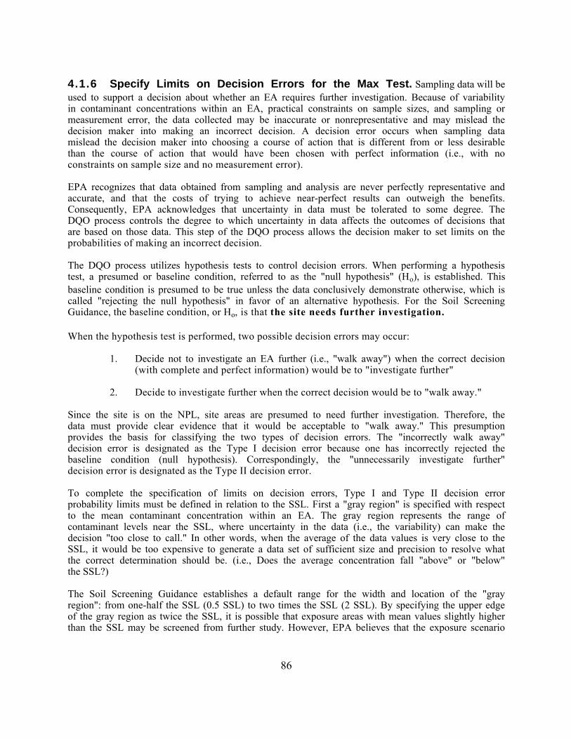
4.1.6 Specify Limits on Decision Errors for the Max Test. Sampling data will beused to support a decision about whether an EA requires further investigation. Because of variabilityin contaminant concentrations within an EA, practical constraints on sample sizes, and sampling ormeasurement error, the data collected may be inaccurate or nonrepresentative and may mislead thedecision maker into making an incorrect decision. A decision error occurs when sampling datamislead the decision maker into choosing a course of action that is different from or less desirablethan the course of action that would have been chosen with perfect information (i.e., with noconstraints on sample size and no measurement error).
EPA recognizes that data obtained from sampling and analysis are never perfectly representative andaccurate, and that the costs of trying to achieve near-perfect results can outweigh the benefits.Consequently, EPA acknowledges that uncertainty in data must be tolerated to some degree. TheDQO process controls the degree to which uncertainty in data affects the outcomes of decisions thatare based on those data. This step of the DQO process allows the decision maker to set limits on theprobabilities of making an incorrect decision.
The DQO process utilizes hypothesis tests to control decision errors. When performing a hypothesistest, a presumed or baseline condition, referred to as the "null hypothesis" (Ho), is established. Thisbaseline condition is presumed to be true unless the data conclusively demonstrate otherwise, which iscalled "rejecting the null hypothesis" in favor of an alternative hypothesis. For the Soil ScreeningGuidance, the baseline condition, or Ho, is that the site needs further investigation.
When the hypothesis test is performed, two possible decision errors may occur:
1. Decide not to investigate an EA further (i.e., "walk away") when the correct decision(with complete and perfect information) would be to "investigate further"
2. Decide to investigate further when the correct decision would be to "walk away."
Since the site is on the NPL, site areas are presumed to need further investigation. Therefore, thedata must provide clear evidence that it would be acceptable to "walk away." This presumptionprovides the basis for classifying the two types of decision errors. The "incorrectly walk away"decision error is designated as the Type I decision error because one has incorrectly rejected thebaseline condition (null hypothesis). Correspondingly, the "unnecessarily investigate further"decision error is designated as the Type II decision error.
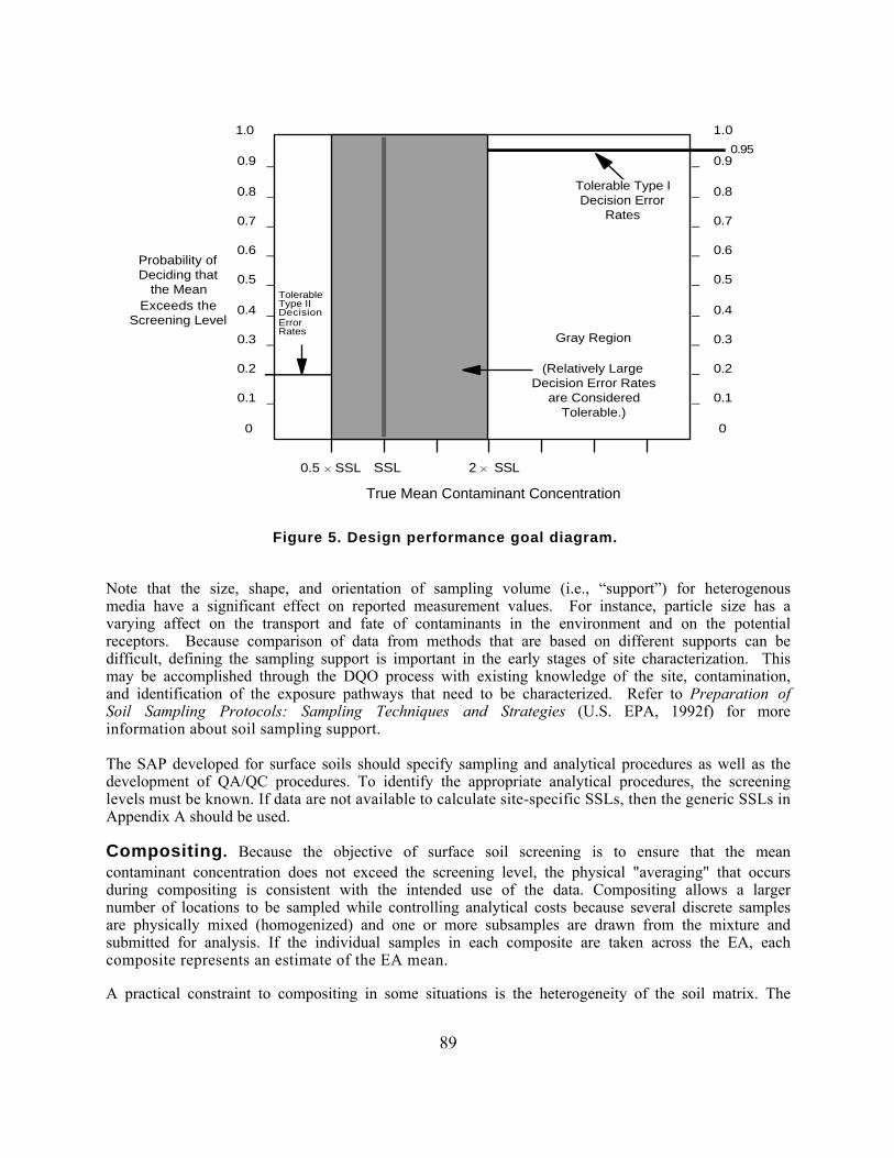
To complete the specification of limits on decision errors, Type I and Type II decision errorprobability limits must be defined in relation to the SSL. First a "gray region" is specified with respectto the mean contaminant concentration within an EA. The gray region represents the range ofcontaminant levels near the SSL, where uncertainty in the data (i.e., the variability) can make thedecision "too close to call." In other words, when the average of the data values is very close to theSSL, it would be too expensive to generate a data set of sufficient size and precision to resolve whatthe correct determination should be. (i.e., Does the average concentration fall "above" or "below"the SSL?)
The Soil Screening Guidance establishes a default range for the width and location of the "grayregion": from one-half the SSL (0.5 SSL) to two times the SSL (2 SSL). By specifying the upper edgeof the gray region as twice the SSL, it is possible that exposure areas with mean values slightly higherthan the SSL may be screened from further study. However, EPA believes that the exposure scenario
86
and assumptions used to derive SSLs are sufficiently conservative to be protective in such cases.
On the lower side of the gray region, the consequences of decision errors at one-half the SSL areprimarily financial. If the lower edge of the gray region were to be moved closer to the SSL, thenmore exposure areas that were truly below the SSL would be screened out, but more money would bespent on sampling to make this determination. If the lower edge of the gray region were to be movedcloser to zero, then less money could be spent on sampling, but fewer EAs that were truly below theSSLs would be screened out, leading to unnecessary investigation of EAs. The Superfund programchose the gray region to be one-half to two times the SSL after investigating several different ranges.This range for the gray region represents a balance between the costs of collecting and analyzing soilsamples and making incorrect decisions. While it is desirable to estimate exactly the exposure areamean, the number of samples required are much more than project managers are generally willing tocollect in a "screening" effort. Although some exposure areas will have contaminant concentrationsthat are between the SSL and twice the SSL and will be screened out, human health will still beprotected given the conservative assumptions used to derive the SSLs.
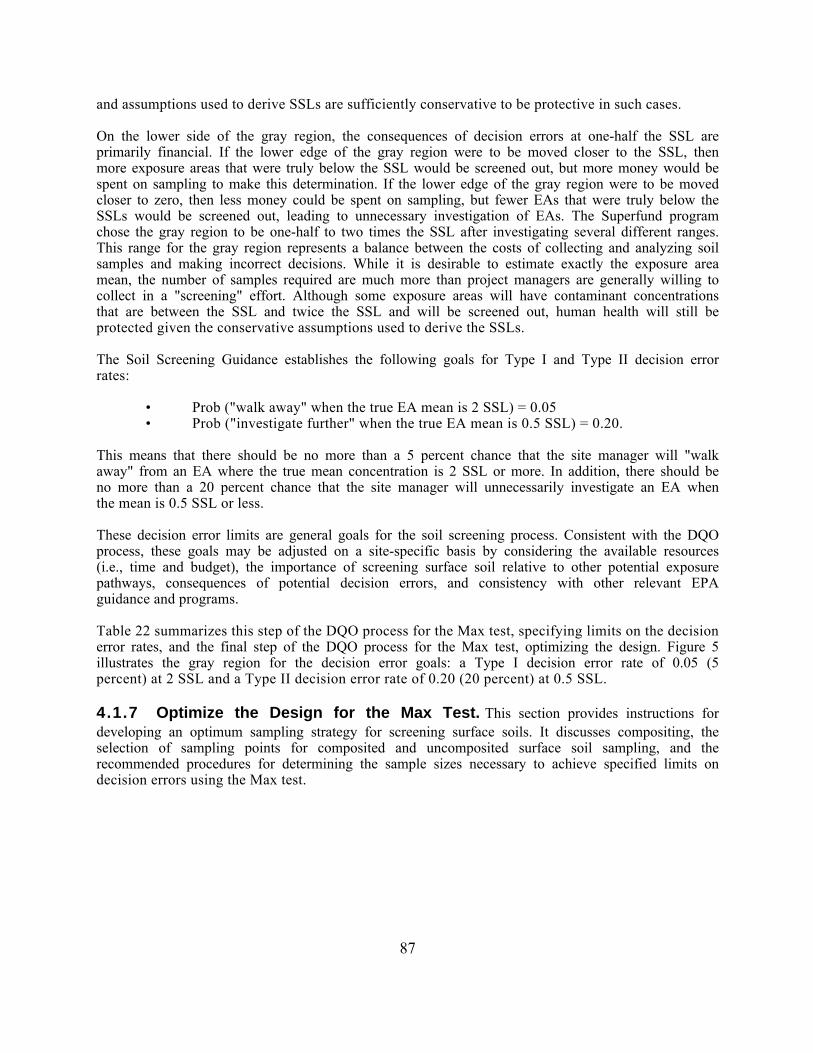
The Soil Screening Guidance establishes the following goals for Type I and Type II decision errorrates:
• Prob ("walk away" when the true EA mean is 2 SSL) = 0.05• Prob ("investigate further" when the true EA mean is 0.5 SSL) = 0.20.
This means that there should be no more than a 5 percent chance that the site manager will "walkaway" from an EA where the true mean concentration is 2 SSL or more. In addition, there should beno more than a 20 percent chance that the site manager will unnecessarily investigate an EA whenthe mean is 0.5 SSL or less.
These decision error limits are general goals for the soil screening process. Consistent with the DQOprocess, these goals may be adjusted on a site-specific basis by considering the available resources(i.e., time and budget), the importance of screening surface soil relative to other potential exposurepathways, consequences of potential decision errors, and consistency with other relevant EPAguidance and programs.
Table 22 summarizes this step of the DQO process for the Max test, specifying limits on the decisionerror rates, and the final step of the DQO process for the Max test, optimizing the design. Figure 5illustrates the gray region for the decision error goals: a Type I decision error rate of 0.05 (5percent) at 2 SSL and a Type II decision error rate of 0.20 (20 percent) at 0.5 SSL.
4.1.7 Optimize the Design for the Max Test. This section provides instructions fordeveloping an optimum sampling strategy for screening surface soils. It discusses compositing, theselection of sampling points for composited and uncomposited surface soil sampling, and therecommended procedures for determining the sample sizes necessary to achieve specified limits ondecision errors using the Max test.
87
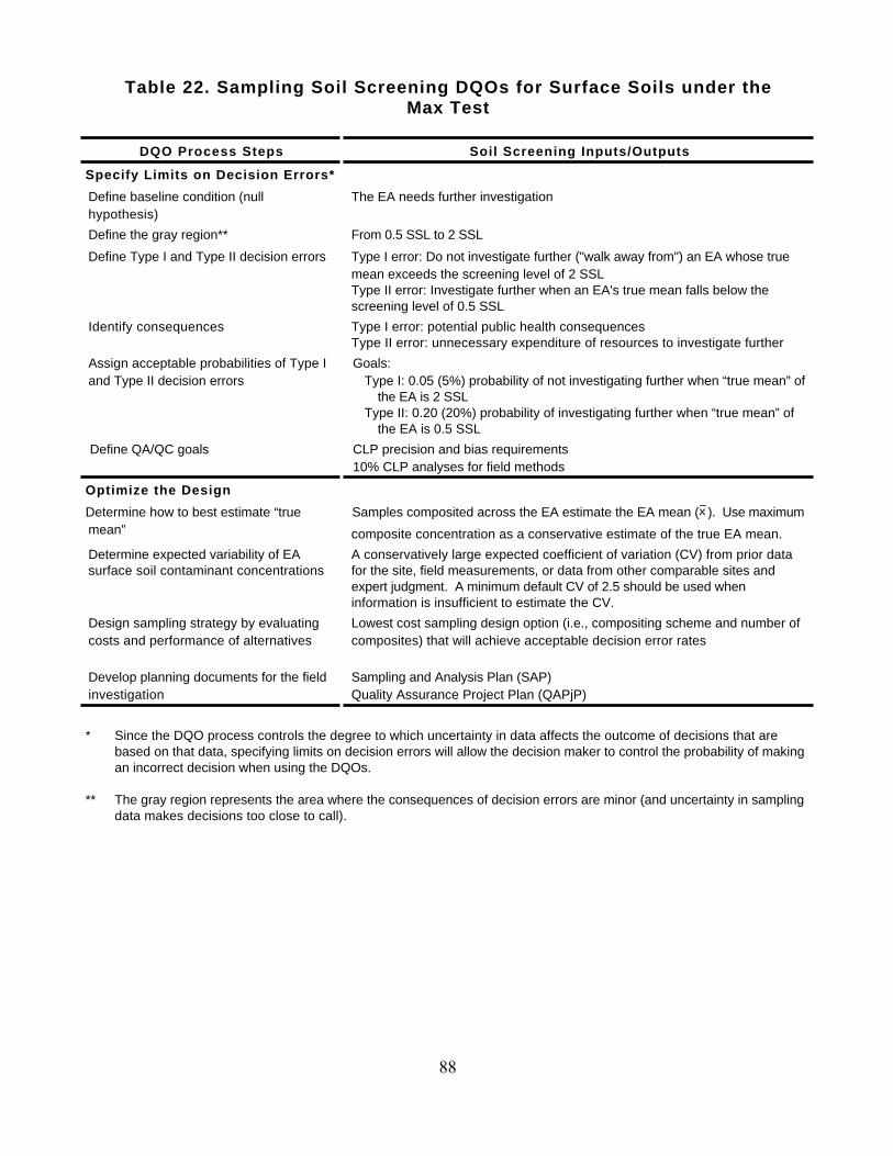
Table 22. Sampling Soil Screening DQOs for Surface Soils under theMax Test
DQO Process Steps Soil Screening Inputs/Outputs
Specify Limits on Decision Errors*
Define baseline condition (nullhypothesis)
The EA needs further investigation
Define the gray region** From 0.5 SSL to 2 SSL
Define Type I and Type II decision errors Type I error: Do not investigate further ("walk away from") an EA whose truemean exceeds the screening level of 2 SSLType II error: Investigate further when an EA's true mean falls below thescreening level of 0.5 SSL
Identify consequences Type I error: potential public health consequencesType II error: unnecessary expenditure of resources to investigate further
Assign acceptable probabilities of Type Iand Type II decision errors
Goals:Type I: 0.05 (5%) probability of not investigating further when “true mean” of
the EA is 2 SSLType II: 0.20 (20%) probability of investigating further when “true mean” of
the EA is 0.5 SSL
Define QA/QC goals CLP precision and bias requirements10% CLP analyses for field methods
Optimize the Design
Determine how to best estimate “truemean”
Samples composited across the EA estimate the EA mean (− x ). Use maximum
composite concentration as a conservative estimate of the true EA mean.
Determine expected variability of EAsurface soil contaminant concentrations
A conservatively large expected coefficient of variation (CV) from prior datafor the site, field measurements, or data from other comparable sites andexpert judgment. A minimum default CV of 2.5 should be used wheninformation is insufficient to estimate the CV.
Design sampling strategy by evaluatingcosts and performance of alternatives
Lowest cost sampling design option (i.e., compositing scheme and number ofcomposites) that will achieve acceptable decision error rates
Develop planning documents for the fieldinvestigation
Sampling and Analysis Plan (SAP)Quality Assurance Project Plan (QAPjP)
* Since the DQO process controls the degree to which uncertainty in data affects the outcome of decisions that arebased on that data, specifying limits on decision errors will allow the decision maker to control the probability of makingan incorrect decision when using the DQOs.
** The gray region represents the area where the consequences of decision errors are minor (and uncertainty in samplingdata makes decisions too close to call).
88
1.0
_ 0.9
_ 0.8
_ 0.7
_ 0.6
_ 0.5
_ 0.4
_ 0.3
_ 0.2
_ 0.1
0
1.0
0.9 _
0.8 _
0.7 _
0.6 _
0.5 _
0.4 _
0.3 _
0.2 _
0.1 _
0
Probability ofDeciding that
the MeanExceeds the
Screening LevelGray Region
(Relatively LargeDecision Error Rates
are ConsideredTolerable.)
0.95
0.5 H SSL SSL 2 H SSL
True Mean Contaminant Concentration
TolerableType IIDecisionErrorRates
Tolerable Type IDecision Error
Rates
Figure 5. Design performance goal diagram.
Note that the size, shape, and orientation of sampling volume (i.e., “support”) for heterogenousmedia have a significant effect on reported measurement values. For instance, particle size has avarying affect on the transport and fate of contaminants in the environment and on the potentialreceptors. Because comparison of data from methods that are based on different supports can bedifficult, defining the sampling support is important in the early stages of site characterization. Thismay be accomplished through the DQO process with existing knowledge of the site, contamination,and identification of the exposure pathways that need to be characterized. Refer to Preparation ofSoil Sampling Protocols: Sampling Techniques and Strategies (U.S. EPA, 1992f) for moreinformation about soil sampling support.
The SAP developed for surface soils should specify sampling and analytical procedures as well as thedevelopment of QA/QC procedures. To identify the appropriate analytical procedures, the screeninglevels must be known. If data are not available to calculate site-specific SSLs, then the generic SSLs inAppendix A should be used.
Compositing. Because the objective of surface soil screening is to ensure that the meancontaminant concentration does not exceed the screening level, the physical "averaging" that occursduring compositing is consistent with the intended use of the data. Compositing allows a largernumber of locations to be sampled while controlling analytical costs because several discrete samplesare physically mixed (homogenized) and one or more subsamples are drawn from the mixture andsubmitted for analysis. If the individual samples in each composite are taken across the EA, eachcomposite represents an estimate of the EA mean.
A practical constraint to compositing in some situations is the heterogeneity of the soil matrix. The
89
efficiency and effectiveness of the mixing process may be hindered when soil particle sizes varywidely or when the soil matrix contains foreign objects, organic matter, viscous fluids, or stickymaterial. Soil samples should not be composited if matrix interference among contaminants is likely(e.g., when the presence of one contaminant biases analytical results for another).
Before individual specimens are composited for chemical analysis, the site manager should considerhomogenizing and splitting each specimen. By compositing one portion of each specimen with theother specimens and storing one portion for potential future analysis, the spatial integrity of eachspecimen is maintained. If the concentration of a contaminant in a composite sample is high, thesplits of the individual specimens from which it was composed can be analyzed discretely todetermine which individual specimen(s) have high concentrations of the contaminant. This willpermit the site manager to determine which portion within an EA is contaminated without making arepeat visit to the site.
Sample Pattern. The Max test should only be applied using composite samples that arerepresentative of the entire EA. However, the Chen test (see Section 4.1.9) can be applied withindividual, uncomposited samples. There are several options for developing a sampling pattern forcompositing that produce samples that should be representative. If individual, uncomposited sampleswill be analyzed for contaminant concentrations, the N sample points can be selected using either (1)simple random sampling (SRS), (2) stratified SRS, or (3) systematic grid sampling (square orrectangular grid) with a random starting point (SyGS/rs). Step-by-step procedures for selecting SRSand SyGS/rs samples are provided in Chapter 5 of the U.S. EPA (1989a) and Chapter 5 of U.S. EPA(1994e). If stratified random sampling is used, the sampling rate must be the same in every sector, orstratum of the EA. Hence, the number of sampling points assigned to a stratum must be directlyproportional to the surface area of the stratum.
Systematic grid sampling with a random starting point is generally preferred because it ensures thatthe sample points will be dispersed across the entire EA. However, if the boundaries of the EA areirregular (e.g., around the perimeter of the site or the boundaries of a stratum within which the EAswere defined), the number of grid sample points that fall within the EA depends on the randomstarting point selected. Therefore, for these irregularly shaped EAs, SRS or stratified SRS isrecommended. Moreover, if a systematic trend of contamination is suspected across the EA (e.g., astrip of higher contamination), then SRS or stratified SRS is recommended again. In this case, gridsampling would be likely to result in either over- or under representation of the strip of highercontaminant levels, depending on the random starting point.
For composite sampling, the sampling pattern used to locate the discrete sample specimens that formeach composite sample (N) is important. The composite samples should be formed in a manner thatis consistent with the assumptions underlying the sample size calculations. In particular, eachcomposite sample should provide an unbiased estimate of the mean contaminant concentration overthe entire EA. One way to construct a valid composite of C specimens is to divide the EA into Csectors, or strata, of equal area and select one point at random from each sector. If sectors (strata)are of unequal sizes, the simple average is no longer representative of the EA as a whole.
Five valid sampling patterns and compositing schemes for selecting N composite samples that eachconsist of C specimens are listed below:
1. Select an SRS consisting of C points and composite all specimens associated with these pointsinto a sample. Repeat this process N times, discarding any points that were used in a previoussample.
90
2. Select an SyGS/rs of C points and composite all specimens associated with the points in thissample. Repeat this process N times, using a new randomly selected starting point each time.
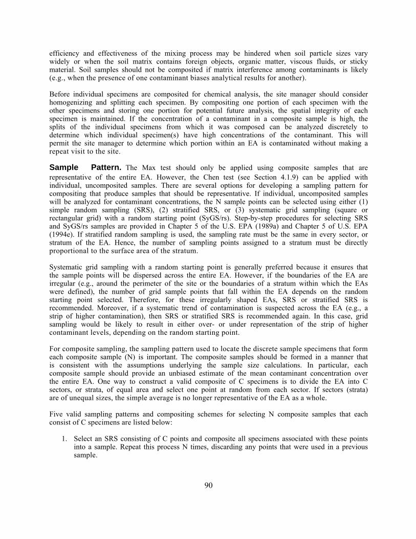
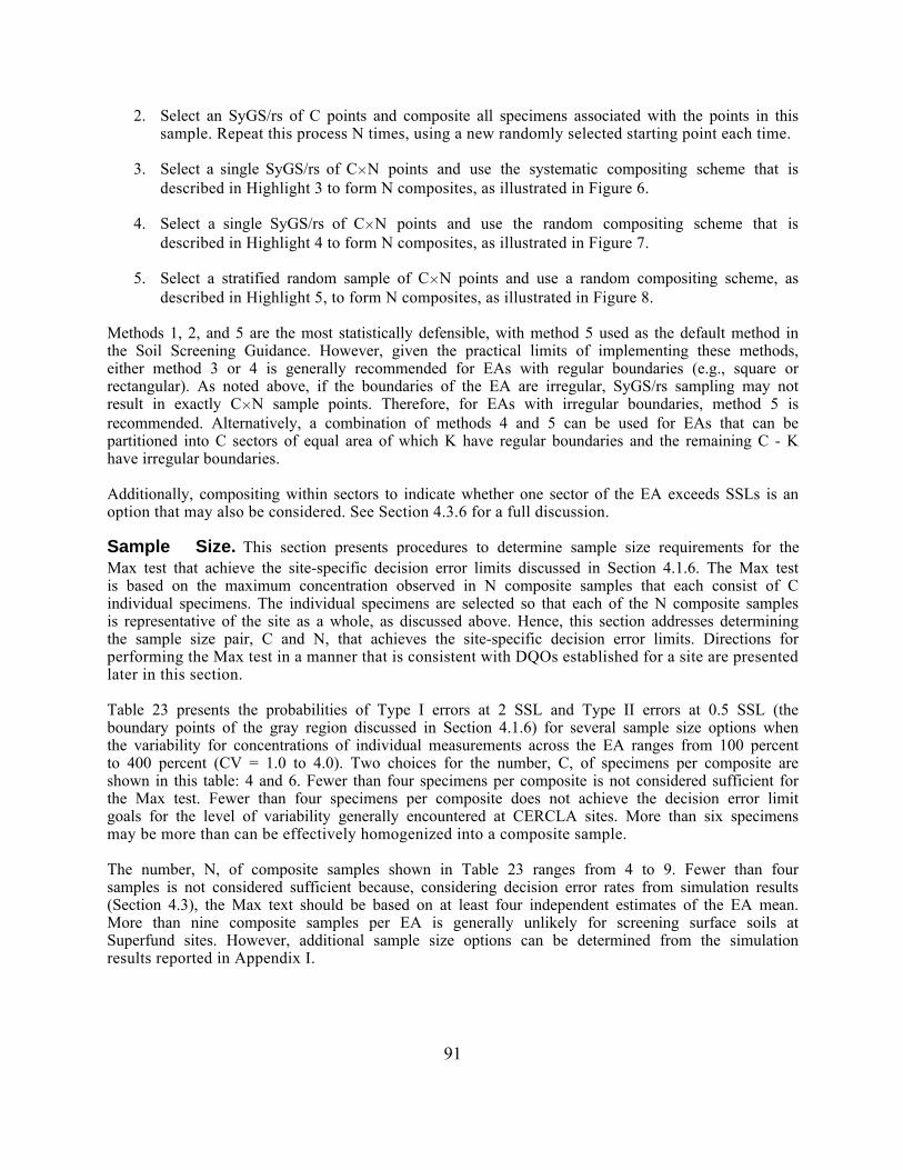
3. Select a single SyGS/rs of CHN points and use the systematic compositing scheme that isdescribed in Highlight 3 to form N composites, as illustrated in Figure 6.
4. Select a single SyGS/rs of CHN points and use the random compositing scheme that isdescribed in Highlight 4 to form N composites, as illustrated in Figure 7.
5. Select a stratified random sample of CHN points and use a random compositing scheme, asdescribed in Highlight 5, to form N composites, as illustrated in Figure 8.
Methods 1, 2, and 5 are the most statistically defensible, with method 5 used as the default method inthe Soil Screening Guidance. However, given the practical limits of implementing these methods,either method 3 or 4 is generally recommended for EAs with regular boundaries (e.g., square orrectangular). As noted above, if the boundaries of the EA are irregular, SyGS/rs sampling may notresult in exactly CHN sample points. Therefore, for EAs with irregular boundaries, method 5 isrecommended. Alternatively, a combination of methods 4 and 5 can be used for EAs that can bepartitioned into C sectors of equal area of which K have regular boundaries and the remaining C - Khave irregular boundaries.
Additionally, compositing within sectors to indicate whether one sector of the EA exceeds SSLs is anoption that may also be considered. See Section 4.3.6 for a full discussion.
Sample Size. This section presents procedures to determine sample size requirements for theMax test that achieve the site-specific decision error limits discussed in Section 4.1.6. The Max testis based on the maximum concentration observed in N composite samples that each consist of Cindividual specimens. The individual specimens are selected so that each of the N composite samplesis representative of the site as a whole, as discussed above. Hence, this section addresses determiningthe sample size pair, C and N, that achieves the site-specific decision error limits. Directions forperforming the Max test in a manner that is consistent with DQOs established for a site are presentedlater in this section.
Table 23 presents the probabilities of Type I errors at 2 SSL and Type II errors at 0.5 SSL (theboundary points of the gray region discussed in Section 4.1.6) for several sample size options whenthe variability for concentrations of individual measurements across the EA ranges from 100 percentto 400 percent (CV = 1.0 to 4.0). Two choices for the number, C, of specimens per composite areshown in this table: 4 and 6. Fewer than four specimens per composite is not considered sufficient forthe Max test. Fewer than four specimens per composite does not achieve the decision error limitgoals for the level of variability generally encountered at CERCLA sites. More than six specimensmay be more than can be effectively homogenized into a composite sample.
The number, N, of composite samples shown in Table 23 ranges from 4 to 9. Fewer than foursamples is not considered sufficient because, considering decision error rates from simulation results(Section 4.3), the Max text should be based on at least four independent estimates of the EA mean.More than nine composite samples per EA is generally unlikely for screening surface soils atSuperfund sites. However, additional sample size options can be determined from the simulationresults reported in Appendix I.
91
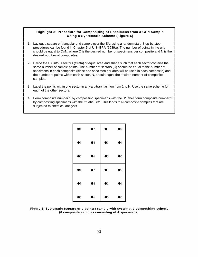
Highlight 3: Procedure for Compositing of Specimens from a Grid Sample Using a Systematic Scheme (Figure 6)
1. Lay out a square or triangular grid sample over the EA, using a random start. Step-by-stepprocedures can be found in Chapter 5 of U.S. EPA (1989a). The number of points in the gridshould be equal to CHN, where C is the desired number of specimens per composite and N is thedesired number of composites.
2. Divide the EA into C sectors (strata) of equal area and shape such that each sector contains thesame number of sample points. The number of sectors (C) should be equal to the number ofspecimens in each composite (since one specimen per area will be used in each composite) andthe number of points within each sector, N, should equal the desired number of compositesamples.
3. Label the points within one sector in any arbitrary fashion from 1 to N. Use the same scheme foreach of the other sectors.
4. Form composite number 1 by compositing specimens with the '1' label, form composite number 2by compositing specimens with the '2' label, etc. This leads to N composite samples that aresubjected to chemical analysis.
l1 l2
l3 l4
l5 l6
l1 l2
l3 l4
l5 l6
l1 l2
l3 l4
l5 l6
l1 l2
l3 l4
l5 l6
Figure 6. Systematic (square grid points) sample with systematic compositing scheme(6 composite samples consisting of 4 specimens).
92
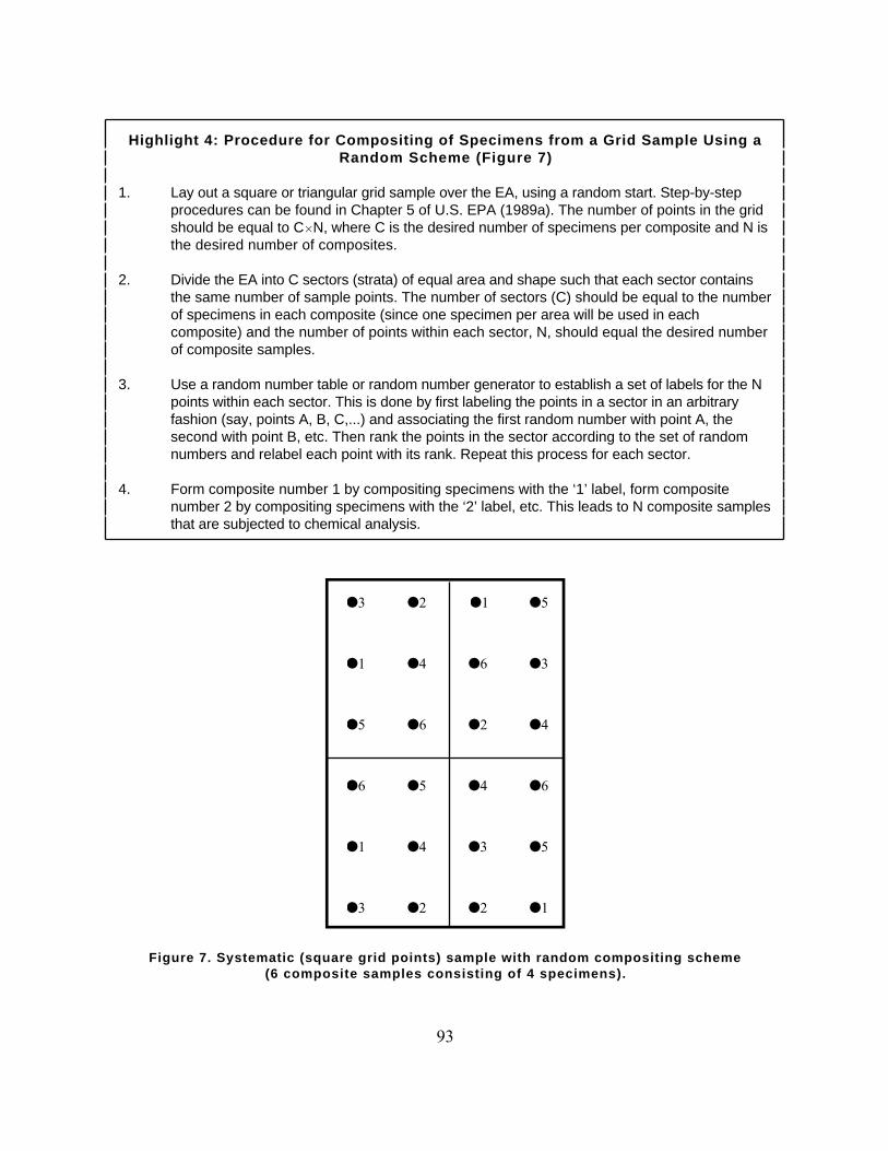
Highlight 4: Procedure for Compositing of Specimens from a Grid Sample Using aRandom Scheme (Figure 7)
1. Lay out a square or triangular grid sample over the EA, using a random start. Step-by-stepprocedures can be found in Chapter 5 of U.S. EPA (1989a). The number of points in the gridshould be equal to CHN, where C is the desired number of specimens per composite and N isthe desired number of composites.
2. Divide the EA into C sectors (strata) of equal area and shape such that each sector containsthe same number of sample points. The number of sectors (C) should be equal to the numberof specimens in each composite (since one specimen per area will be used in eachcomposite) and the number of points within each sector, N, should equal the desired numberof composite samples.
3. Use a random number table or random number generator to establish a set of labels for the Npoints within each sector. This is done by first labeling the points in a sector in an arbitraryfashion (say, points A, B, C,...) and associating the first random number with point A, thesecond with point B, etc. Then rank the points in the sector according to the set of randomnumbers and relabel each point with its rank. Repeat this process for each sector.
4. Form composite number 1 by compositing specimens with the ‘1’ label, form compositenumber 2 by compositing specimens with the ‘2’ label, etc. This leads to N composite samplesthat are subjected to chemical analysis.
l3 l2
l1 l4
l5 l6
l1 l5
l6 l3
l2 l4
l6 l5
l1 l4
l3 l2
l4 l6
l3 l5
l2 l1
Figure 7. Systematic (square grid points) sample with random compositing scheme(6 composite samples consisting of 4 specimens).
93
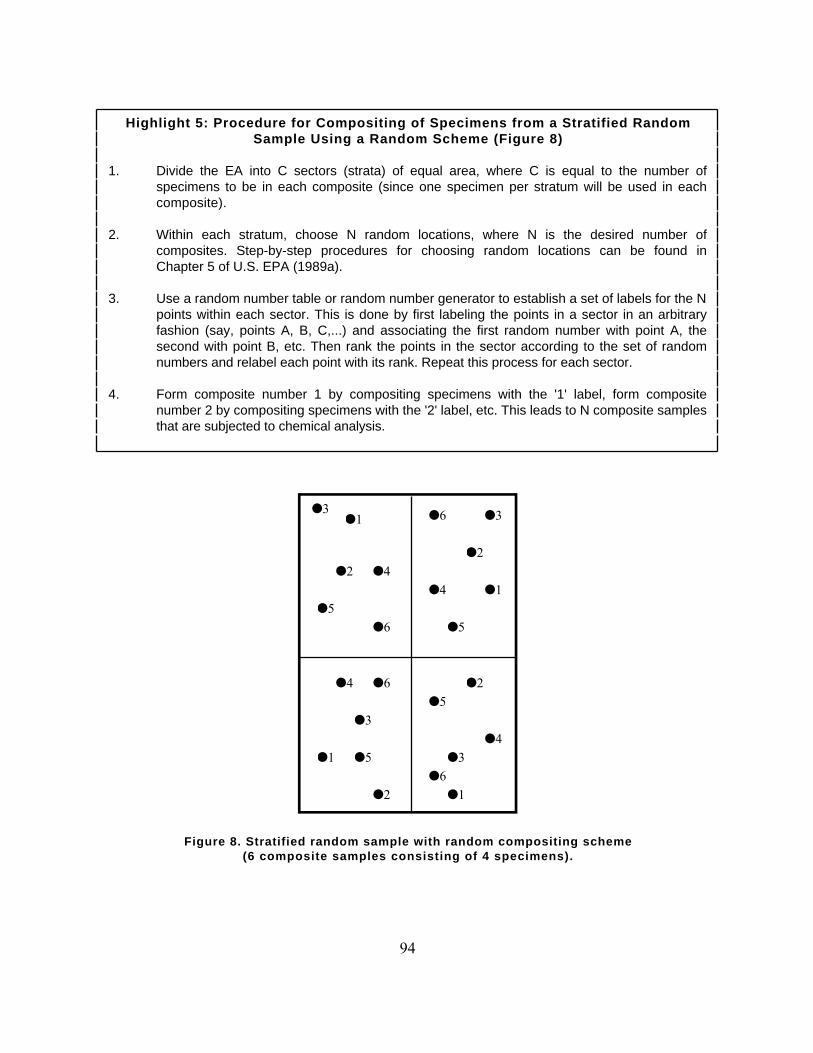
Highlight 5: Procedure for Compositing of Specimens from a Stratified RandomSample Using a Random Scheme (Figure 8)
1. Divide the EA into C sectors (strata) of equal area, where C is equal to the number ofspecimens to be in each composite (since one specimen per stratum will be used in eachcomposite).
2. Within each stratum, choose N random locations, where N is the desired number ofcomposites. Step-by-step procedures for choosing random locations can be found inChapter 5 of U.S. EPA (1989a).
3. Use a random number table or random number generator to establish a set of labels for the Npoints within each sector. This is done by first labeling the points in a sector in an arbitraryfashion (say, points A, B, C,...) and associating the first random number with point A, thesecond with point B, etc. Then rank the points in the sector according to the set of randomnumbers and relabel each point with its rank. Repeat this process for each sector.
4. Form composite number 1 by compositing specimens with the '1' label, form compositenumber 2 by compositing specimens with the '2' label, etc. This leads to N composite samplesthat are subjected to chemical analysis.
l1
l2
l3
l4
l5
l6
l1
l2
l3
l4
l5
l6
l1
l2
l3
l4
l5
l6
l1
l2
l3
l4
l5
l6
Figure 8. Stratified random sample with random compositing scheme(6 composite samples consisting of 4 specimens).
94
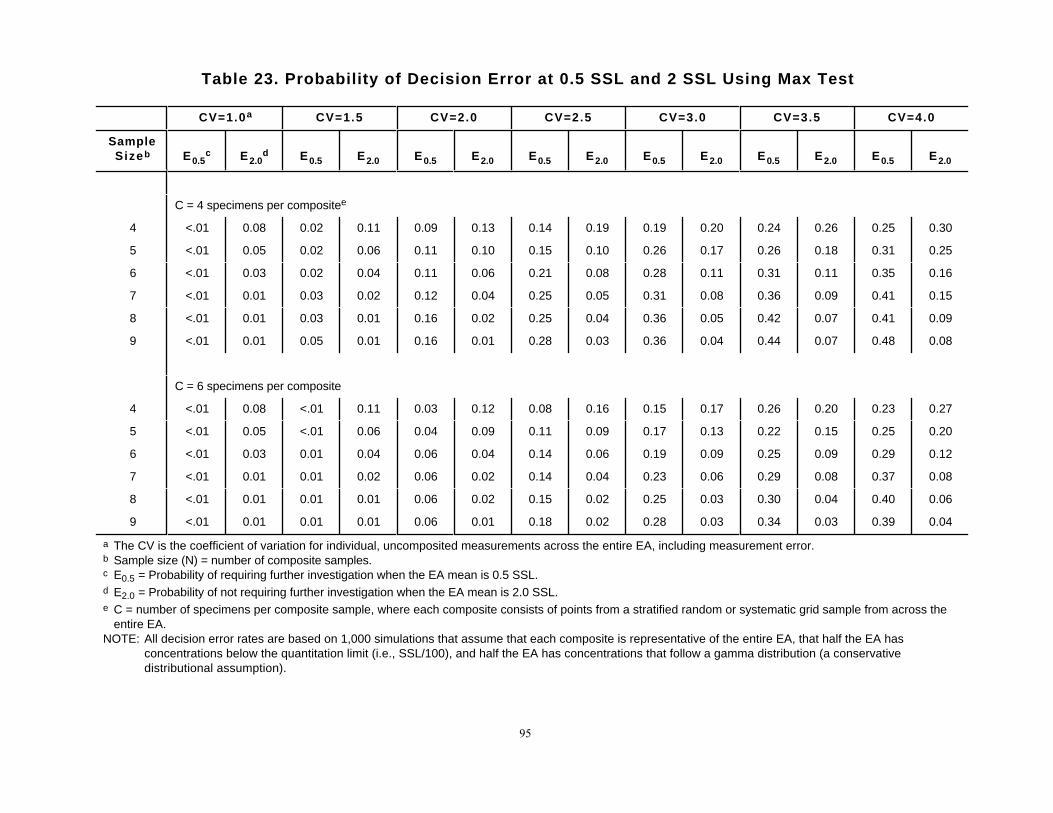
Table 23. Probability of Decision Error at 0.5 SSL and 2 SSL Using Max Test
CV=1.0a CV=1.5 CV=2.0 CV=2.5 CV=3.0 CV=3.5 CV=4.0
SampleSizeb E0.5
c E2.0d E0.5 E2.0 E0.5 E2.0 E0.5 E2.0 E0.5 E2.0 E0.5 E2.0 E0.5 E2.0
C = 4 specimens per compositee
4 <.01 0.08 0.02 0.11 0.09 0.13 0.14 0.19 0.19 0.20 0.24 0.26 0.25 0.30
5 <.01 0.05 0.02 0.06 0.11 0.10 0.15 0.10 0.26 0.17 0.26 0.18 0.31 0.25
6 <.01 0.03 0.02 0.04 0.11 0.06 0.21 0.08 0.28 0.11 0.31 0.11 0.35 0.16
7 <.01 0.01 0.03 0.02 0.12 0.04 0.25 0.05 0.31 0.08 0.36 0.09 0.41 0.15
8 <.01 0.01 0.03 0.01 0.16 0.02 0.25 0.04 0.36 0.05 0.42 0.07 0.41 0.09
9 <.01 0.01 0.05 0.01 0.16 0.01 0.28 0.03 0.36 0.04 0.44 0.07 0.48 0.08
C = 6 specimens per composite
4 <.01 0.08 <.01 0.11 0.03 0.12 0.08 0.16 0.15 0.17 0.26 0.20 0.23 0.27
5 <.01 0.05 <.01 0.06 0.04 0.09 0.11 0.09 0.17 0.13 0.22 0.15 0.25 0.20
6 <.01 0.03 0.01 0.04 0.06 0.04 0.14 0.06 0.19 0.09 0.25 0.09 0.29 0.12
7 <.01 0.01 0.01 0.02 0.06 0.02 0.14 0.04 0.23 0.06 0.29 0.08 0.37 0.08
8 <.01 0.01 0.01 0.01 0.06 0.02 0.15 0.02 0.25 0.03 0.30 0.04 0.40 0.06
9 <.01 0.01 0.01 0.01 0.06 0.01 0.18 0.02 0.28 0.03 0.34 0.03 0.39 0.04
a The CV is the coefficient of variation for individual, uncomposited measurements across the entire EA, including measurement error. b Sample size (N) = number of composite samples. c E0.5 = Probability of requiring further investigation when the EA mean is 0.5 SSL. d E2.0 = Probability of not requiring further investigation when the EA mean is 2.0 SSL. e C = number of specimens per composite sample, where each composite consists of points from a stratified random or systematic grid sample from across the
entire EA. NOTE: All decision error rates are based on 1,000 simulations that assume that each composite is representative of the entire EA, that half the EA has
concentrations below the quantitation limit (i.e., SSL/100), and half the EA has concentrations that follow a gamma distribution (a conservativedistributional assumption).
95
The error rates shown in Table 23 are based on the simulations presented in Appendix I. Thesesimulations are based on the following assumptions:
1. Each of the N composite samples is based on C specimens selected to berepresentative of the EA as a whole, as specified above (C = number of sectors orstrata).
2. One-half the EA has concentrations below the quantitation limit (which is assumed tobe SSL/100).
3. One-half the EA has concentrations that follow a gamma distribution (see Section 4.3for additional discussion).
4. Each chemical analysis is subject to a 20 percent measurement error.
The error rates presented in Table 23 are based on the above assumptions which make them robustfor most potential distributions of soil contaminant concentrations. Distribution assumptions 2 and 3were used because they were found in the simulations to produce high error rates relative to otherpotential contaminant distributions (see Section 4.3). If the proportion of the site below thequantitation limit (QL) is less than half or if the distribution of the concentration measurements issome other distribution skewed to the right (e.g., lognormal), rather than gamma, then the error ratesachieved are likely to be no worse than those cited in Table 23. Although the actual contaminantdistribution may be different from those cited above as the basis for Table 23, only extensiveinvestigations will usually generate sufficient data to determine the actual distribution for each EA.
Using Table 23 to determine the sample size pair (C and N) needed to achieve satisfactory error rateswith the Max test requires an a priori estimate of the coefficient of variation for measurements ofthe contaminant of interest across the EA. The coefficient of variation (CV) is the ratio of thestandard deviation of contaminant concentrations for individual, uncomposited specimens divided bythe EA mean concentration. As discussed in Section 4.1.4, the EAs should be constructed withinstrata expected to have relatively homogeneous concentrations so that an estimate of the CV for astratum may be applicable for all EAs in that stratum. The site manager should use a conservativelylarge estimate of the CV for determining sample size requirements because additional sampling will beneeded if the data suggest that the true CV is greater than that used to determine the sample sizes.
Potential sources of information for estimating the EA or stratum means, variances, and CVs includethe following (in descending order of desirability):
• Data from a pilot study conducted at the site• Prior sampling data from the site• Data from similar sites• Professional judgment.
For more information on estimating variability, see Section 6.3.1 of U.S. EPA (1989a).
4.1.8 Using the DQA Process: Analyzing Max Test Data. This section providesguidance for analyzing the data for the Max test.
The hypothesis test for the Max test is very simple to implement, which is one reason that the Maxtest is attractive as a surface soil screening test. If x1, x2, ..., xN represent concentrationmeasurements for N composite samples that each consist of C specimens selected so that each
96
composite is representative of the EA as a whole (as described in Section 4.1.7), the Max test isimplemented as follows:
If Max (x1, x2, ..., xN) $ 2 SSL, then investigate the EA further; If Max (x1, x2, ..., xN) < 2 SSL, and the data quality assessment (DQA) indicates that thesample size was adequate, then no further investigation is necessary.
In addition, the step-by-step procedures presented in Highlight 6 must be implemented to ensure thatthe site-specific error limits, as discussed in Section 4.1.6, are achieved.
If the EA mean is below 2 SSL, the DQA process may be used to determine if the sample size wassufficiently large to justify the decision to not investigate further. To use Table 23 to check whetherthe sample size is adequate, an estimate of the CV is needed for each EA. The first four steps ofHighlight 6, the DQA process for the Max test, present a process for the computation of a sampleCV for an EA based on the N composite samples that each consist of C specimens.
However, the sample CV can be quite large when all the measurements are very small (e.g., well belowthe SSL) because CV approaches infinity as the EA sample mean (− x ) approaches zero. Thus, whenthe composite concentration values for an EA are all near zero, the sample CV may be questionableand therefore unreliable for determining if the original sample size was sufficient (i.e., it could lead tofurther sampling when the EA mean is well below 2 SSL). To protect against unnecessary additionalsampling in such cases, compare all composites against the equation given in Step 5 of Highlight 6. Ifthe maximum composite sample concentration is below the value given by the equation, then thesample size may be assumed to be adequate and no further DQA is necessary.
To develop Step 5, EPA decided that if there were no compositing (C=1) and all the observations(based on a sample size appropriate for a CV of 2.5) were less than the SSL, then one can reasonablyassume that the EA mean was not greater than 2 SSL. Likewise, because the standard error for themean of C specimens, as represented by the composite sample, is proportional to 1/ C , thecomparable condition for composite observations is that one can reasonably assume that the EAmean was not greater than 2 SSL when all composite observations were less than SSL/ C . If this isthe case for an EA sample set, the sample size can be assumed to be adequate and no further DQA isneeded. Otherwise (when at lease one composite observation is not this small), use Table 23 with thesample CV for the EA to determine whether a sufficient number of samples were taken to achieveDQOs.
In addition to being simple to implement, the Max test is recommended because it provides goodcontrol over the Type I error rates at 2 SSL with small sample sizes. It also does not need anyassumptions regarding observations below the QL. Moreover, the Max test error rates at 2 SSL arefairly robust against alternative assumptions regarding the distribution of surface soil concentrationsin the EA. The simulations in Appendix I show that these error rates are rather stable for lognormalor Weibull contaminant concentration distributions and for different assumptions about portions ofthe site with contaminant concentrations below the QL.
97
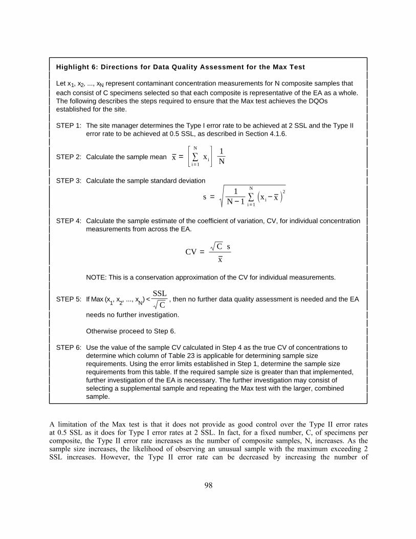
Highlight 6: Directions for Data Quality Assessment for the Max Test
Let x1, x2, ..., xN represent contaminant concentration measurements for N composite samples thateach consist of C specimens selected so that each composite is representative of the EA as a whole.The following describes the steps required to ensure that the Max test achieves the DQOsestablished for the site.
STEP 1: The site manager determines the Type I error rate to be achieved at 2 SSL and the Type IIerror rate to be achieved at 0.5 SSL, as described in Section 4.1.6.
STEP 2: Calculate the sample mean − x = N
3 i = 1
x i 1 N
STEP 3: Calculate the sample standard deviation
s = 1
N − 1
N
3 i = 1
x i − − x 2
STEP 4: Calculate the sample estimate of the coefficient of variation, CV, for individual concentrationmeasurements from across the EA.
CV = C s− x
NOTE: This is a conservation approximation of the CV for individual measurements.
STEP 5: If Max (x1, x
2, ..., x
N) <
SSL
C , then no further data quality assessment is needed and the EA
needs no further investigation.
Otherwise proceed to Step 6.
STEP 6: Use the value of the sample CV calculated in Step 4 as the true CV of concentrations todetermine which column of Table 23 is applicable for determining sample sizerequirements. Using the error limits established in Step 1, determine the sample sizerequirements from this table. If the required sample size is greater than that implemented,further investigation of the EA is necessary. The further investigation may consist ofselecting a supplemental sample and repeating the Max test with the larger, combinedsample.
A limitation of the Max test is that it does not provide as good control over the Type II error ratesat 0.5 SSL as it does for Type I error rates at 2 SSL. In fact, for a fixed number, C, of specimens percomposite, the Type II error rate increases as the number of composite samples, N, increases. As thesample size increases, the likelihood of observing an unusual sample with the maximum exceeding 2SSL increases. However, the Type II error rate can be decreased by increasing the number of
98
specimens per composite. This unusual performance of the Max test as a hypothesis testingprocedure occurs because the rejection region is fixed below 2 SSL and thus does not depend on thesample size (as it does for typical hypothesis testing procedures).
4.1.9 Specify Limits on Decision Errors for Chen Test. Although the Max test isadequate and appropriate for selecting a sample size for site screening, there are other alternatemethods of screening surface soils. One such alternate method is the Chen test. In general, the Chentest differs from the Max test in its basic assumption about site contamination and the purpose ofsoil sampling. Because of this variation, these two methods have different null hypotheses anddifferent decision error types.
There are two formulations of the statistical hypothesis test concerning the true (but unknown)mean contaminant concentration, µ, that achieve the Soil Screening Guidance decision error rategoals specified in Section 4.1.6. They are:
1. Test the null hypothesis, H0: µ ≥ 2 SSL, versus the alternative hypothesis,H1: µ < 2 SSL, at the 5 percent significance level using a sample size chosen toachieve a Type II error rate of 20 percent at 0.5 SSL.
2. Test the null hypothesis, H0: µ ≤ 0.5 SSL, versus the alternative hypothesis,H1: µ > 0.5 SSL, at the 20 percent significance level using a sample size chosen toachieve a Type II error rate of 5 percent at 2 SSL.
The first formulation of the problem (which is commonly used in the Superfund program) has theadvantage that the error rate that has potential public health consequences is controlled directly viathe significance level of the test. The error rate that has primarily cost consequences can be reducedby increasing the sample size above the minimum requirement. However, EPA has identified a newtest procedure, the Chen test (Chen, 1995), which requires the second formulation but is less sensitiveto assumptions regarding the distribution of the contaminant measurements than the Land procedureused in the December 1994 draft Technical Background Document (see Section 4.3). This sectionprovides guidance regarding application of the Chen test and is, therefore, based on the secondformulation of the hypothesis test.
A disadvantage of the second formulation is its performance when the true EA mean is between 0.5SSL and the SSL. In this case, as the sample size increases, the test indicates the decision toinvestigate further, even though the mean is less than the SSL. In fact, no test procedure with feasiblesample sizes performs well when the true EA mean is in the "gray region" between 0.5 SSL and 2 SSL(see Section 4.3). Whenever large sample sizes are feasible, one should modify the problem statementand test the null hypothesis, H0: µ ≤ SSL, instead of H0: µ ≤ 0.5 SSL. One would then developappropriate DQOs for this modified hypothesis test (e.g., significance level of 20 percent at the SSLand 5 percent probability of decision error at 2 SSL).
When the true mean of an EA is compared with the screening level, there are two possible decisionerrors that may occur: (1) decide not to investigate an EA further (i.e., "walk away") when thecorrect decision would be to "investigate further"; and (2) decide to investigate further when thecorrect decision would be to "walk away." For the Chen test, the "incorrectly walk away" decisionerror is designated as the Type II decision error because it occurs when we incorrectly accept the nullhypothesis. Correspondingly, the "unnecessarily investigate further" decision error is designated asthe Type I decision error because it occurs when we incorrectly reject the null hypothesis.
99
As discussed in Section 4.1.6, the Soil Screening Guidance specifies a default gray region for decisionerrors from 0.5 SSL to 2 SSL and sets the following goals for Type I and Type II error rates:
• Prob ("investigate further" when the true EA mean is 0.5 SSL) = 0.20• Prob ("walk away" when the true EA mean is 2 SSL) = 0.05.
Table 24 summarizes this step of the DQO process for the Chen test, specifying limits on thedecision error rates, and the final step of the DQO process, optimizing the design.
4.1.10 Optimize the Design Using the Chen Test. This section includes guidance ondeveloping an optimum sampling strategy for screening surface soils. It discusses compositing, theselection of sampling points for composited and uncomposited surface soil sampling, and therecommended procedures for determining the sample sizes necessary to achieve specified limits ondecision errors using the Chen test.
Note that the size, shape, and orientation of sampling volume (i.e., “support”) for heterogenousmedia have a significant effect on reported measurement values. For instance, particle size has avarying affect on the transport and fate of contaminants in the environment and on the potentialreceptors. Because comparison of data from methods that are based on different supports can bedifficult, defining the sampling support is important in the early stages of site characterization. Thismay be accomplished through the DQO process with existing knowledge of the site, contamination,and identification of the exposure pathways that need to be characterized. Refer to Preparation ofSoil Sampling Protocols: Sampling Techniques and Strategies (U.S. EPA, 1992f) for moreinformation about soil sampling support.
The SAP developed for surface soils should specify sampling and analytical procedures as well as thedevelopment of QA/QC procedures. To identify the appropriate analytical procedures, the screeninglevels must be known. If data are not available to calculate site-specific SSLs, then the generic SSLs inAppendix A should be used.
Compositing. Because the objective of surface soil screening is to ensure that the meancontaminant concentration does not exceed the screening level, the physical "averaging" that occursduring compositing is consistent with the intended use of the data. Compositing allows a largernumber of locations to be sampled while controlling analytical costs because several discrete samplesare physically mixed (homogenized) and one or more subsamples are drawn from the mixture andsubmitted for analysis. If the individual samples in each composite are taken across the EA, eachcomposite represents an estimate of the EA mean.
A practical constraint to compositing in some situations is the heterogeneity of the soil matrix. Theefficiency and effectiveness of the mixing process may be hindered when soil particle sizes varywidely or when the soil matrix contains foreign objects, organic matter, viscous fluids, or stickymaterial. Soil samples should not be composited if matrix interference among contaminants is likely(e.g., when the presence of one contaminant biases analytical results for another).
100
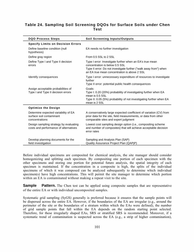
Table 24. Sampling Soil Screening DQOs for Surface Soils under ChenTest
DQO Process Steps Soil Screening Inputs/Outputs
Specify Limits on Decision Errors
Define baseline condition (nullhypothesis)
EA needs no further investigation
Define gray region From 0.5 SSL to 2 SSL
Define Type I and Type II decisionerrors
Type I error: Investigate further when an EA's true meanconcentration is below 0.5 SSL Type II error: Do not investigate further ("walk away from") whenan EA true mean concentration is above 2 SSL
Identify consequences Type I error: unnecessary expenditure of resources to investigatefurther Type II error: potential public health consequences
Assign acceptable probabilities of Type I and Type II decision errors
Goals:Type I: 0.20 (20%) probability of investigating further when EAmean is 0.5 SSL Type II: 0.05 (5%) probability of not investigating further when EAmean is 2 SSL
Optimize the Design
Determine expected variability of EAsurface soil contaminantconcentrations
A conservatively large expected coefficient of variation (CV) fromprior data for the site, field measurements, or data from othercomparable sites and expert judgment
Design sampling strategy by evaluatingcosts and performance of alternatives
Lowest cost sampling design option (i.e., compositing schemeand number of composites) that will achieve acceptable decisionerror rates
Develop planning documents for thefield investigation
Sampling and Analysis Plan (SAP)Quality Assurance Project Plan (QAPjP)
Before individual specimens are composited for chemical analysis, the site manager should considerhomogenizing and splitting each specimen. By compositing one portion of each specimen with theother specimens and storing one portion for potential future analysis, the spatial integrity of eachspecimen is maintained. If the concentration in a composite is high, the splits of the individualspecimens of which it was composed can be analyzed subsequently to determine which individualspecimen(s) have high concentrations. This will permit the site manager to determine which portionwithin an EA is contaminated without making a repeat visit to the site.
Sample Pattern. The Chen test can be applied using composite samples that are representativeof the entire EA or with individual uncomposited samples.
Systematic grid sampling (SyGS) generally is preferred because it ensures that the sample points willbe dispersed across the entire EA. However, if the boundaries of the EA are irregular (e.g., around theperimeter of the site or the boundaries of a stratum within which the EAs were defined), the numberof grid sample points that fall within the EA depends on the random starting point selected.Therefore, for these irregularly shaped EAs, SRS or stratified SRS is recommended. Moreover, if asystematic trend of contamination is suspected across the EA (e.g., a strip of higher contamination),
101
then SRS or stratified SRS is recommended again. In this case, grid sampling would be likely to resultin either over- or under representation of the strip of higher contaminant levels, depending on therandom starting point.
For composite sampling, the sampling pattern used to locate the C discrete sample specimens thatform each composite sample is important. The composite samples must be formed in a manner thatis consistent with the assumptions underlying the sample size calculations. In particular, eachcomposite sample must provide an unbiased estimate of the mean contaminant concentration overthe entire EA. One way to construct a valid composite of C specimens is to divide the EA into Csectors, or strata, of equal area and select one point at random from each sector. If sectors (strata)are of unequal sizes, the simple average is no longer representative of the EA as a whole.
Valid sampling patterns and compositing schemes for selecting N composite samples that eachconsist of C specimens include the following:
1. Select an SRS consisting of C points and composite all specimens associated withthese points into a sample. Repeat this process N times, discarding any points thatwere used in a previous sample.
2. Select an SyGS/rs of C points and composite all specimens associated with the pointsin this sample. Repeat this process N times, using a new randomly selected startingpoint each time.
3. Select a single SyGS/rs of CN points and use the systematic compositing scheme thatis described in Highlight 3 to form N composites, as illustrated in Figure 6.
4. Select a single SyGS/rs of CHN points and use the random compositing scheme that isdescribed in Highlight 4 to form N composites, as illustrated in Figure 7.
5. Select a stratified random sample of CHN points and use a random compositingscheme, as described in Highlight 5, to form N composites, as illustrated in Figure 8.
Methods 1, 2, and 5 are the most statistically defensible, with method 5 used as the default method inthe Soil Screening Guidance. However, given the practical limits of implementing these methods,either method 3 or 4 is generally recommended for EAs with regular boundaries (e.g., square orrectangular). As noted above, if the boundaries of the EA are irregular, SyGS/rs sampling may notresult in exactly CHN sample points. Therefore, for EAs with irregular boundaries, method 5 isrecommended. Alternatively, a combination of methods 4 and 5 can be used for EAs that can bepartitioned into C sectors of equal area of which K have regular boundaries and the remaining C - Khave irregular boundaries.
Sample Size. This section provides procedures to determine sample size requirements for theChen test that achieve the site-specific decision error limits discussed in Section 4.1.6. The Chen testis an upper-tail test for the mean of positively skewed distributions, like the lognormal (Chen, 1995).It is based on the mean concentration observed in a simple random sample, or equivalent design,selected from a distribution with a long right-hand tail.
The Chen procedure is a hypothesis testing procedure that is robust among the family of right-skewed distributions (see Section 4.3). That is, decision error rates for a given sample size arerelatively insensitive to the particular right-skewed distribution that generated the data. This
102
robustness is important in the context of surface soil screening because the number of surface soilsamples will usually not be sufficient to determine the distribution of the concentrationmeasurements.
The procedures presented above for selecting composited or uncomposited simple random orsystematic grid samples can all be used to generate samples for application of the Chen test. TheChen procedure is based on a simple random sample, or one that can be analyzed as if it were an SRS.Directions for performing the Chen test in a manner that is consistent with the DQOs that have beenestablished for a site are presented later.
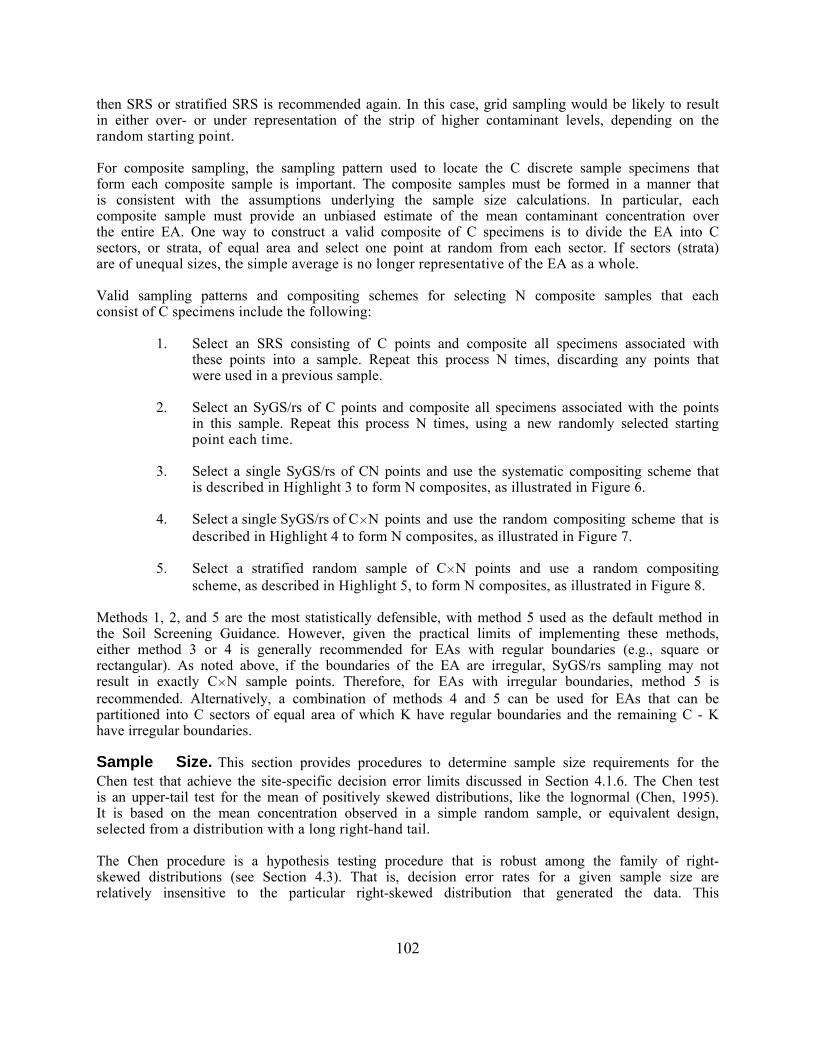
Tables 25 through 30 provide the sample sizes required for the Chen test performed at the 10, 20, or40 percent levels of significance (probability of Type I error at 0.5 SSL) and achieve, at most, a 5 or10 percent probability of (Type II) error at 2 SSL. The Type II error rates at 2 SSL are based on thesimulations presented in Appendix I. These simulations are based on the following assumptions:
1. Each of the N composite samples is based on C specimens selected to berepresentative of the EA as a whole, as specified above.
2. One-half the EA has concentrations below the quantitation limit (which is assumed tobe SSL/100).
3. One-half the EA has concentrations that follow a gamma distribution.
4. Measurements below the QL are replaced by 0.5 QL for computation of the Chen teststatistic.
5. Each chemical analysis is subject to a 20 percent measurement error.
Distributional assumptions 2 and 3 were used as the basis for the Type II error rates at 2 SSL (shownin Tables 25 through 30) because they were found in the simulations to produce high error ratesrelative to other potential contaminant distributions. If the proportion of the site below the QL isless than half or if the distribution of the concentration measurements is some other right-skeweddistribution (e.g., lognormal), rather than gamma, then the Type II error rates achieved are likely tobe no worse than those cited in Tables 25 through 30. No sample sizes, N, less than four are shown inthese tables (irrespective of the number of specimens per composite) because consideration of thesimulation results presented in Section 4.3 has led to a program-level decision that at least fourseparate analyses are required to adequately characterize the mean of an EA. No sample sizes inexcess of nine are presented because of a program-level decision that more than nine samples perexposure area is generally unlikely for screening surface soils at Superfund sites. However, additionalsample size options can be determined from the simulations reported in Appendix I.
When using Tables 25 through 30 to determine the sample size pair (C and N) needed to achievesatisfactory error rates with the Chen test, investigators must have an a priori estimate of the CV formeasurements of the contaminant of interest across the EA. As previously discussed for the Maxtest, the site manager should use a conservatively large estimate of the CV for determining samplesize requirements because additional sampling will be required if the data suggest that the true CV isgreater than that used to determine the sample sizes.
103
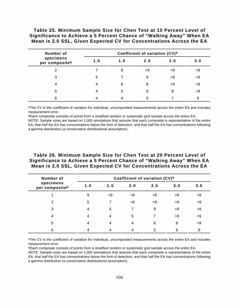
Table 25. Minimum Sample Size for Chen Test at 10 Percent Level ofSignificance to Achieve a 5 Percent Chance of “Walking Away” When EAMean is 2.0 SSL, Given Expected CV for Concentrations Across the EA
Number ofspecimens
per compositeb
Coefficient of variation (CV)a
1 .0 1 .5 2 .0 2 .5 3 .0
2 7 9 >9 >9 >9
3 5 7 9 >9 >9
4 4 6 8 >9 >9
5 4 5 6 8 >9
6 4 4 5 7 9
aThe CV is the coefficient of variation for individual, uncomposited measurements across the entire EA and includesmeasurement error. bEach composite consists of points from a stratified random or systematic grid sample across the entire EA. NOTE: Sample sizes are based on 1,000 simulations that assume that each composite is representative of the entireEA, that half the EA has concentrations below the limit of detection, and that half the EA has concentrations followinga gamma distribution (a conservative distributional assumption).
Table 26. Minimum Sample Size for Chen Test at 20 Percent Level ofSignificance to Achieve a 5 Percent Chance of “Walking Away” When EAMean is 2.0 SSL, Given Expected CV for Concentrations Across the EA
Number ofspecimens
per compositeb
Coefficient of variation (CV)a
1 .0 1 .5 2 .0 2 .5 3 .0 3 .5
1 9 >9 >9 >9 >9 >9
2 5 7 >9 >9 >9 >9
3 4 5 7 9 >9 >9
4 4 4 6 7 >9 >9
5 4 4 4 6 8 >9
6 4 4 4 5 8 9
aThe CV is the coefficient of variation for individual, uncomposited measurements across the entire EA and includesmeasurement error. bEach composite consists of points from a stratified random or systematic grid sample across the entire EA. NOTE: Sample sizes are based on 1,000 simulations that assume that each composite is representative of the entireEA, that half the EA has concentrations below the limit of detection, and that half the EA has concentrations followinga gamma distribution (a conservative distributional assumption).
104
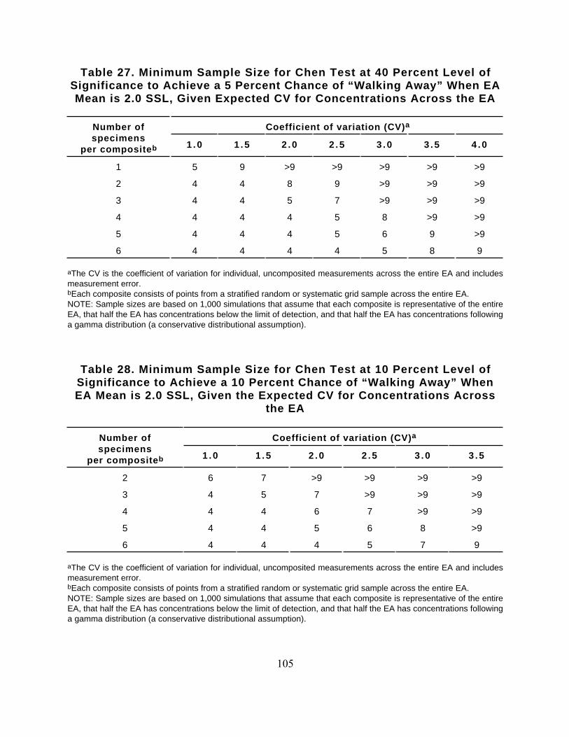
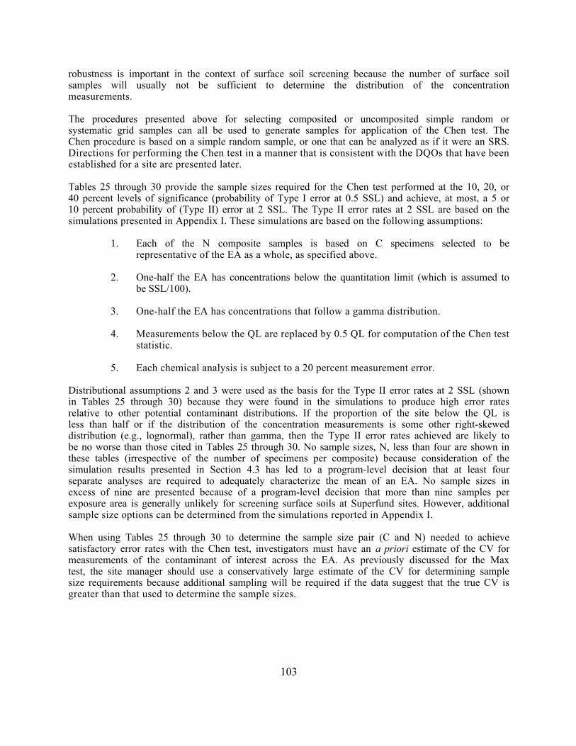
Table 27. Minimum Sample Size for Chen Test at 40 Percent Level ofSignificance to Achieve a 5 Percent Chance of “Walking Away” When EAMean is 2.0 SSL, Given Expected CV for Concentrations Across the EA
Number ofspecimens
per compositeb
Coefficient of variation (CV)a
1 .0 1 .5 2 .0 2 .5 3 .0 3 .5 4 .0
1 5 9 >9 >9 >9 >9 >9
2 4 4 8 9 >9 >9 >9
3 4 4 5 7 >9 >9 >9
4 4 4 4 5 8 >9 >9
5 4 4 4 5 6 9 >9
6 4 4 4 4 5 8 9
aThe CV is the coefficient of variation for individual, uncomposited measurements across the entire EA and includesmeasurement error. bEach composite consists of points from a stratified random or systematic grid sample across the entire EA. NOTE: Sample sizes are based on 1,000 simulations that assume that each composite is representative of the entireEA, that half the EA has concentrations below the limit of detection, and that half the EA has concentrations followinga gamma distribution (a conservative distributional assumption).
Table 28. Minimum Sample Size for Chen Test at 10 Percent Level ofSignificance to Achieve a 10 Percent Chance of “Walking Away” WhenEA Mean is 2.0 SSL, Given the Expected CV for Concentrations Across
the EA
Number ofspecimens
per compositeb
Coefficient of variation (CV)a
1 .0 1 .5 2 .0 2 .5 3 .0 3 .5
2 6 7 >9 >9 >9 >9
3 4 5 7 >9 >9 >9
4 4 4 6 7 >9 >9
5 4 4 5 6 8 >9
6 4 4 4 5 7 9
aThe CV is the coefficient of variation for individual, uncomposited measurements across the entire EA and includesmeasurement error. bEach composite consists of points from a stratified random or systematic grid sample across the entire EA. NOTE: Sample sizes are based on 1,000 simulations that assume that each composite is representative of the entireEA, that half the EA has concentrations below the limit of detection, and that half the EA has concentrations followinga gamma distribution (a conservative distributional assumption).
105
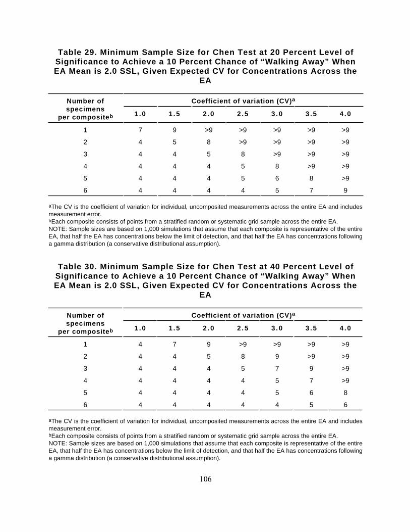
Table 29. Minimum Sample Size for Chen Test at 20 Percent Level ofSignificance to Achieve a 10 Percent Chance of “Walking Away” WhenEA Mean is 2.0 SSL, Given Expected CV for Concentrations Across the
EA
Number ofspecimens
per compositeb
Coefficient of variation (CV)a
1 .0 1 .5 2 .0 2 .5 3 .0 3 .5 4 .0
1 7 9 >9 >9 >9 >9 >9
2 4 5 8 >9 >9 >9 >9
3 4 4 5 8 >9 >9 >9
4 4 4 4 5 8 >9 >9
5 4 4 4 5 6 8 >9
6 4 4 4 4 5 7 9
aThe CV is the coefficient of variation for individual, uncomposited measurements across the entire EA and includesmeasurement error. bEach composite consists of points from a stratified random or systematic grid sample across the entire EA. NOTE: Sample sizes are based on 1,000 simulations that assume that each composite is representative of the entireEA, that half the EA has concentrations below the limit of detection, and that half the EA has concentrations followinga gamma distribution (a conservative distributional assumption).
Table 30. Minimum Sample Size for Chen Test at 40 Percent Level ofSignificance to Achieve a 10 Percent Chance of “Walking Away” WhenEA Mean is 2.0 SSL, Given Expected CV for Concentrations Across the
EA
Number ofspecimens
per compositeb
Coefficient of variation (CV)a
1 .0 1 .5 2 .0 2 .5 3 .0 3 .5 4 .0
1 4 7 9 >9 >9 >9 >9
2 4 4 5 8 9 >9 >9
3 4 4 4 5 7 9 >9
4 4 4 4 4 5 7 >9
5 4 4 4 4 5 6 8
6 4 4 4 4 4 5 6
aThe CV is the coefficient of variation for individual, uncomposited measurements across the entire EA and includesmeasurement error. bEach composite consists of points from a stratified random or systematic grid sample across the entire EA. NOTE: Sample sizes are based on 1,000 simulations that assume that each composite is representative of the entireEA, that half the EA has concentrations below the limit of detection, and that half the EA has concentrations followinga gamma distribution (a conservative distributional assumption).
106
Given an a priori estimate of the CV of concentration measurements in the EA, the site manager canuse Table 26 to determine a sample size option that achieves the decision error goals for surface soilscreening presented in Section 4.1.6 (i.e., not more than 20 percent chance of error at 0.5 SSL andnot more than 5 percent at 2 SSL). For example, suppose that the site manager expects that themaximum true CV for concentration measurements in an EA is 2. Then Table 26 shows that sixcomposite samples, each consisting of four specimens, will be sufficient to achieve the decision errorlimit goals.
4.1.11 Using the DQA Process: Analyzing Chen Test Data. Step-by-stepinstructions for using the Chen test to analyze data from both discrete random samples and pseudo-random samples (e.g., composite samples constructed as described previously) are provided inHighlight 7. This method for analyzing the data is a robust procedure for an upper-tailed test for themean of a positively skewed distribution. As explained by Chen (1995), this procedure is a robustgeneralization of the familiar Student's t-test; it further generalizes a method developed by Johnson(1978) for asymmetric distributions.
The only assumption necessary for valid application of the Chen procedure is that the sample be arandom sample from a right-skewed distribution. This robustness within the broad family of right-skewed distributions is appropriate for screening surface soil because the distribution ofconcentrations within an EA may depart from the common assumption of lognormality.
Computation of the Chen test statistic, as shown in Highlight 7, requires that concentration values beavailable for all N individual or composite samples analyzed for the contaminant of interest. If ananalytical test result is reported below the quantitation limit, it should be used in the computations.For results below detection, substitute one-half the QL.
A disadvantage of the Chen procedure is that the hypothesis, “the EA needs no furtherinvestigation,” must be treated as the alternative hypothesis, rather than as the null hypothesis. As aresult, the Type I error rate at 0.5 SSL is controlled via the significance level of the test, rather thanthe error rate at 2 SSL, which may have public health consequences. Hence, if the sample sizes (C andN) are based on an assumed CV that is too small, the desired error rate at 2 SSL is likely not to beachieved. Therefore, it is important to perform the data quality assurance check specified in Steps 6through 8 of Highlight 7 to ensure that the desired error rate at 2 SSL is achieved. Moreover, it isimportant that the site manager base the initial EA sample sizes on a conservatively large estimateof the CV so that this process will not result in the need for additional sampling.
4.1.12 Special Considerations for Multiple Contaminants. If the surface soilsamples collected for an EA will be tested for multiple contaminants, be aware that the expected CVsfor the different contaminants may not all be identical. A conservative approach is to base thesample sizes for all contaminants on the largest expected CV.
4.1.13 Quality Assurance/Quality Control Requirements. Regardless of thesampling approach used, the Superfund quality assurance program guidance must be followed to ensurethat measurement error rates are documented and within acceptable limits (U.S. EPA, 1993d).
107
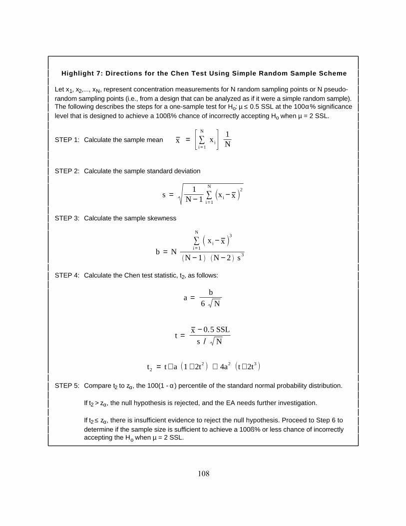
Highlight 7: Directions for the Chen Test Using Simple Random Sample Scheme
Let x1, x2,..., xN, represent concentration measurements for N random sampling points or N pseudo-random sampling points (i.e., from a design that can be analyzed as if it were a simple random sample).The following describes the steps for a one-sample test for Ho: µ ≤ 0.5 SSL at the 100α% significancelevel that is designed to achieve a 100ß% chance of incorrectly accepting Ho when µ = 2 SSL.
STEP 1: Calculate the sample mean − x = N
3 i = 1
x i 1 N
STEP 2: Calculate the sample standard deviation
s = 1
N − 1
N
3 i = 1
x i − − x 2
STEP 3: Calculate the sample skewness
b = N
N
3 i = 1
x i − − x 3
N − 1 N − 2 s 3
STEP 4: Calculate the Chen test statistic, t2, as follows:
a = b
6 N
t = − x − 0 . 5 SSL
s / N
t 2 = t + a 1 + 2 t 2 + 4 a 2 t + 2 t 3
STEP 5: Compare t2 to zα, the 100(1 - α) percentile of the standard normal probability distribution.
If t2 > zα, the null hypothesis is rejected, and the EA needs further investigation.
If t2 ≤ zα, there is insufficient evidence to reject the null hypothesis. Proceed to Step 6 todetermine if the sample size is sufficient to achieve a 100ß% or less chance of incorrectlyaccepting the Ho when µ = 2 SSL.
108
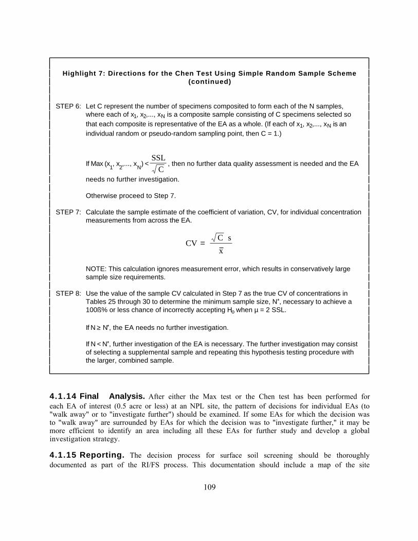
Highlight 7: Directions for the Chen Test Using Simple Random Sample Scheme(continued)
STEP 6: Let C represent the number of specimens composited to form each of the N samples,where each of x1, x2,..., xN is a composite sample consisting of C specimens selected sothat each composite is representative of the EA as a whole. (If each of x1, x2,..., xN is anindividual random or pseudo-random sampling point, then C = 1.)
If Max (x1, x
2,..., x
N) <
SSL
C , then no further data quality assessment is needed and the EA
needs no further investigation.
Otherwise proceed to Step 7.
STEP 7: Calculate the sample estimate of the coefficient of variation, CV, for individual concentrationmeasurements from across the EA.
CV = C s− x
NOTE: This calculation ignores measurement error, which results in conservatively largesample size requirements.
STEP 8: Use the value of the sample CV calculated in Step 7 as the true CV of concentrations inTables 25 through 30 to determine the minimum sample size, N*, necessary to achieve a100ß% or less chance of incorrectly accepting Ho when µ = 2 SSL.
If N ≥ N*, the EA needs no further investigation.
If N < N*, further investigation of the EA is necessary. The further investigation may consistof selecting a supplemental sample and repeating this hypothesis testing procedure withthe larger, combined sample.
4.1.14 Final Analysis. After either the Max test or the Chen test has been performed foreach EA of interest (0.5 acre or less) at an NPL site, the pattern of decisions for individual EAs (to"walk away" or to "investigate further") should be examined. If some EAs for which the decision wasto "walk away" are surrounded by EAs for which the decision was to "investigate further," it may bemore efficient to identify an area including all these EAs for further study and develop a globalinvestigation strategy.
4.1.15 Reporting. The decision process for surface soil screening should be thoroughlydocumented as part of the RI/FS process. This documentation should include a map of the site
109
(showing the boundaries of the EAs and the sectors, or strata, within EAs that were used to selectsampling points within the EAs); documentation of how composite samples were formed and thenumber of composite samples that were analyzed for each EA; the raw analytical data; the results ofall hypothesis tests; and the results of all QA/QC analyses.
4.2 Sampling Subsurface Soils
Subsurface soil sampling is conducted to estimate the mean concentrations of contaminants in eachsource at a site for comparison to inhalation and migration to ground water SSLs. Measurements ofsoil properties and estimates of the area and depth of contamination in each source are also neededto calculate SSLs for these pathways. Table 31 shows the steps in the DQO process necessary todevelop a sampling strategy to meet these objectives. Each of these steps is described below.
4.2.1 State the Problem. Contaminants present in subsurface soils at the site may posesignificant risk to human health and the environment through the inhalation of volatiles or by themigration of contaminants through soils to an underlying potable aquifer. The problem is to identifythe contaminants and source areas that do not pose significant risk to human health through eitherof these exposure pathways so that future investigations may be focused on areas and contaminantsof true concern.
Site-specific activities in this step include identifying the data collection planning team (includingtechnical experts and key stakeholders) and specifying the available resources (i.e., the cost and timeavailable for sampling). The list of technical experts and stakeholders should contain all keypersonnel who are involved with applying SSLs to the site. Other activities include developing theconceptual site model and identifying exposure scenarios, which are fully addressed in the SoilScreening Guidance: User’s Guide (U.S. EPA, 1996).
4.2.2 Identify the Decision. The decision is to determine whether mean soilconcentrations in each source area exceed inhalation or migration to ground water SSLs for specificcontaminants. If so, the source area will be investigated further. If not, no further action will betaken under CERCLA.
4.2.3 Identify Inputs to the Decision. Site-specific inputs to the decision include theaverage contaminant concentrations within each source area and the inhalation and migration groundwater SSLs. Calculation of the SSLs for the two pathways of concern also requires site-specificmeasurements of soil properties (i.e., bulk density, fraction organic carbon content, pH, and soiltexture class) and estimates of the areal extent and depth of contamination.
A list of feasible sampling and analytical methods should be assembled during this step. EPArecommends the use of field methods where applicable and appropriate. Verify that ContractLaboratory Program (CLP) methods and field methods for analyzing the samples exist and that theanalytical method detection limits or field method detection limits are appropriate for the site-specific or generic SSL. The Sampler's Guide to the Contract Laboratory Program (U.S. EPA, 1990)and the User's Guide to the Contract Laboratory Program (U.S. EPA, 1991d) contain furtherinformation on CLP methods.
110
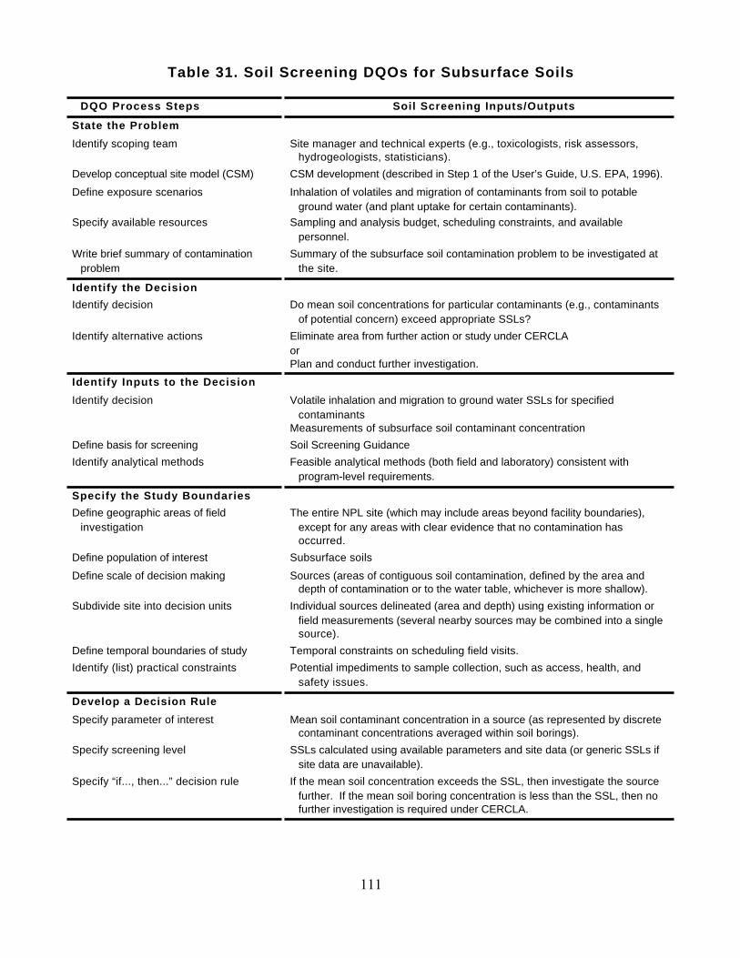
Table 31. Soil Screening DQOs for Subsurface Soils
DQO Process Steps Soil Screening Inputs/Outputs
State the Problem
Identify scoping team Site manager and technical experts (e.g., toxicologists, risk assessors,hydrogeologists, statisticians).
Develop conceptual site model (CSM) CSM development (described in Step 1 of the User’s Guide, U.S. EPA, 1996).
Define exposure scenarios Inhalation of volatiles and migration of contaminants from soil to potableground water (and plant uptake for certain contaminants).
Specify available resources Sampling and analysis budget, scheduling constraints, and availablepersonnel.
Write brief summary of contaminationproblem
Summary of the subsurface soil contamination problem to be investigated atthe site.
Identify the Decision
Identify decision Do mean soil concentrations for particular contaminants (e.g., contaminantsof potential concern) exceed appropriate SSLs?
Identify alternative actions Eliminate area from further action or study under CERCLAorPlan and conduct further investigation.
Identify Inputs to the Decision
Identify decision Volatile inhalation and migration to ground water SSLs for specifiedcontaminants
Measurements of subsurface soil contaminant concentration
Define basis for screening Soil Screening Guidance
Identify analytical methods Feasible analytical methods (both field and laboratory) consistent withprogram-level requirements.
Specify the Study Boundaries
Define geographic areas of fieldinvestigation
The entire NPL site (which may include areas beyond facility boundaries),except for any areas with clear evidence that no contamination hasoccurred.
Define population of interest Subsurface soils
Define scale of decision making Sources (areas of contiguous soil contamination, defined by the area anddepth of contamination or to the water table, whichever is more shallow).
Subdivide site into decision units Individual sources delineated (area and depth) using existing information orfield measurements (several nearby sources may be combined into a singlesource).
Define temporal boundaries of study Temporal constraints on scheduling field visits.
Identify (list) practical constraints Potential impediments to sample collection, such as access, health, andsafety issues.
Develop a Decision Rule
Specify parameter of interest Mean soil contaminant concentration in a source (as represented by discretecontaminant concentrations averaged within soil borings).
Specify screening level SSLs calculated using available parameters and site data (or generic SSLs ifsite data are unavailable).
Specify “if..., then...” decision rule If the mean soil concentration exceeds the SSL, then investigate the sourcefurther. If the mean soil boring concentration is less than the SSL, then nofurther investigation is required under CERCLA.
111
Table 31. (continued)
Specify Limits on Decision Errors
Define QA/QC goals CLP precision and bias requirements10% CLP analyses for field methods
Optimize the Design
Determine how to estimate meanconcentration in a source
For each source, the highest mean soil core concentration (i.e., depth-weighted average of discrete contaminant concentrations within a boring).
Define subsurface sampling strategy byevaluating costs and site-specificconditions
Number of soil borings per source area; number of sampling intervals withdepth.
Develop planning documents for the fieldinvestigation
Sampling and Analysis Plan (SAP)Quality Assurance Project Plan (QAPjP)
Field methods will be useful in defining the study boundaries (i.e., area and depth of contamination)during site reconnaissance and during the sampling effort. For example, soil gas survey is an idealmethod for determining the extent of volatile contamination in the subsurface. EPA expects fieldmethods will become more prevalent and useful because the design and capabilities of field portableinstrumentation are rapidly evolving. Documents on standard operating procedures (SOPs) for fieldmethods are available through NTIS and should be referenced in soil screening documentation if thesemethods are used.
Soil parameters necessary for SSL calculation are soil texture, bulk density, and soil organic carbon.Some of these parameters can be measured in the field, others require laboratory measurement.Although laboratory measurements of these parameters cannot be obtained under the SuperfundContract Laboratory Program, they are readily available from soil testing laboratories across thecountry.
Note that the size, shape, and orientation of sampling volume (i.e., “support”) for heterogenousmedia have a significant effect on reported measurement values. For instance, particle size has avarying affect on the transport and fate of contaminants in the environment and on the potentialreceptors. Comparison of data from methods that are based on different supports can be difficult.Defining the sampling support is important in the early stages of site characterization. This may beaccomplished through the DQO process with existing knowledge of the site, contamination, andidentification of the exposure pathways that need to be characterized. Refer to Preparation of SoilSampling Protocols: Sampling Techniques and Strategies (U.S. EPA, 1992f) for more informationabout soil sampling support.
Soil Texture. The soil texture class (e.g., loam, sand, silt loam) is necessary to estimate average soilmoisture conditions and to estimate infiltration rates. A soil's texture classification is determinedfrom a particle size analysis and the U.S. Department of Agriculture (USDA) soil textural triangleshown at the top of Figure 9. This classification system is based on the USDA soil particle sizeclassification at the bottom of Figure 9. The particle size analysis method in Gee and Bauder (1986)can provide this particle size distribution also. Other particle size analysis methods may be used aslong as they provide the same particle size breakpoints for sand/silt (0.05 mm) and silt/clay(0.002 mm). Field methods are an alternative for determining soil textural class; an example fromBrady (1990) is also presented in Figure 9.
112
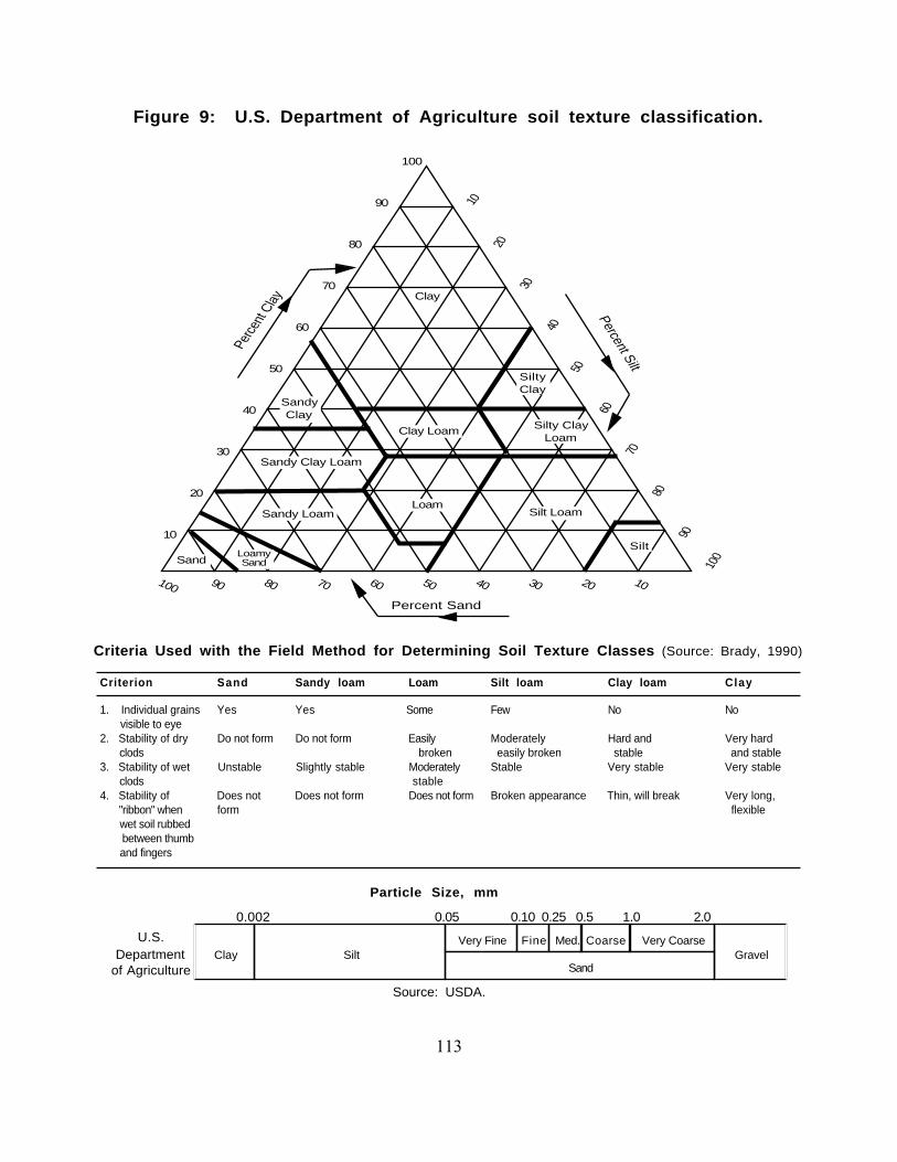
Criteria Used with the Field Method for Determining Soil Texture Classes (Source: Brady, 1990)
Criterion Sand Sandy loam Loam Silt loam Clay loam Clay
1. Individual grains Yes Yes Some Few No No visible to eye2. Stability of dry Do not form Do not form Easily Moderately Hard and Very hard clods broken easily broken stable and stable3. Stability of wet Unstable Slightly stable Moderately Stable Very stable Very stable clods stable4. Stability of Does not Does not form Does not form Broken appearance Thin, will break Very long, "ribbon" when form flexible wet soil rubbed between thumb and fingers
0.002 0.05 0.10 0.25 0.5 1.0 2.0
U.S.Department
of Agriculture
Very Fine
Fine
Med.
Coarse
Very Coarse
Silt
Sand
Clay
Gravel
Particle Size, mm
Source: USDA.
Figure 9: U.S. Department of Agriculture soil texture classification.
Clay
100
90
80
70
60
50
40
30
20
10
100
90
80
70
60
50
40
30
20
10
10 20
30 40
50 60
70 80
90 100
Clay Loam
Sandy Clay Loam
SandyClay
SiltyClay
Silty ClayLoam
Sandy Loam
Sand
LoamySand
Loam
Silt
Percent Silt
Percent Sand
Perc
ent C
lay
Silt Loam
113
Dry Bulk Density. Dry soil bulk density (ρb) is used to calculate total soil porosity and can bedetermined for any soil horizon by weighing a thin-walled tube soil sample (e.g., Shelby tube) ofknown volume and subtracting the tube weight to estimate field bulk density (ASTM D 2937). Amoisture content determination (ASTM 2216) is then made on a subsample of the tube sample toadjust field bulk density to dry bulk density. The other methods (e.g., ASTM D 1556, D 2167, D2922) are not generally applicable to subsurface soils. ASTM soil testing methods are readilyavailable in the Annual Book of ASTM Standards, Volume 4.08, Soil and Rock; Building Stones,which is available from ASTM, 100 Barr Harbor Drive, West Conshohocken, PA, 19428.
Organic Carbon and pH. Soil organic carbon is measured by burning off soil carbon in a controlled-temperature oven (Nelson and Sommers, 1982). This parameter is used to determine soil-waterpartition coefficients from the organic carbon soil-water partition coefficient, Koc. Soil pH is used toselect site-specific partition coefficients for metals and ionizing organic compounds (see Part 5).This simple measurement is made with a pH meter in a soil/water slurry (McLean, 1982) and may bemeasured in the field using a portable pH meter.
4.2.4 Define the Study Boundaries. As discussed in Section 4.1.4, areas that are knownto be highly contaminated (i.e., sources) are targeted for subsurface sampling. The informationcollected on source area and depth is used to calculate site-specific SSLs for the inhalation andmigration to ground water pathways. Contamination is defined by the lower of the CLP practicalquantitation limit for each contaminant or the SSL. For the purposes of this guidance, source areasare defined by area and depth as contiguous zones of contamination. However, discrete sources thatare near each other may be combined and investigated as a single source if site conditions warrant.
4.2.5 Develop a Decision Rule. The decision rule for subsurface soils is:
If the mean concentration of a contaminant within a source area exceeds thescreening level, then investigate that area further.
In this case "screening level" means the SSL. As explained in Section 4.1.5, statistics other than themean (e.g., the maximum concentration) may be used as estimates of the mean in this comparison aslong as they represent valid or conservative estimates of the mean.
4.2.6 Specify Limits on Decision Errors. EPA recognizes that data obtained fromsampling and analysis can never be perfectly representative or accurate and that the costs of tryingto achieve near-perfect results can outweigh the benefits. Consequently, EPA acknowledges thatuncertainty in data must be tolerated to some degree. The DQO process attempts to control thedegree to which uncertainty in data affects the outcomes of decisions that are based on data.
The sampling intensity necessary to accurately determine the mean concentration of subsurface soilcontamination within a source with a specified level of confidence (e.g., 95 percent) is impracticablefor screening due to excessive costs and difficulties with implementation. Therefore, EPA hasdeveloped an alternative decision rule based on average concentrations within individual soil corestaken in a source:
If the mean concentration within any soil core taken in a source exceeds thescreening level, then investigate that source further.
114
For each core, the mean core concentration is defined as the depth-weighted average concentrationwithin the zone of contamination (see Section 4.2.7). Since the soil cores are taken in the area(s) ofhighest contamination within each source, the highest average core concentration among a set ofcore samples serves as a conservative estimate of the mean source concentration. Because this rule isnot a statistical decision, it is not possible to statistically define limits on decision errors.
Standard limits on the precision and bias of sampling and analytical operations conducted during thesampling program do apply. These are specified by the Superfund quality assurance programrequirements (U.S. EPA, 1993d), which must be followed during the subsurface sampling effort.
If field methods are used, at least 10 percent of field samples should be split and sent to a CLPlaboratory for confirmatory analysis (U.S. EPA, 1993d).
Although the EPA does not require full CLP sample tracking and quality assurance/quality control(QA/QC) procedures for measurement of soil properties, routine EPA QA/QC procedures arerecommended, including a Quality Assurance Project Plan (QAPjP), chain-of-custody forms, andduplicate analyses.
4.2.7 Optimize the Design. Within each source, the Soil Screening Guidance suggeststaking two to three soil cores using split spoon or Shelby tube samplers. For each soil core, samplesshould begin at the ground surface and continue at approximately 2-foot intervals until nocontamination is encountered or to the water table, whichever is shallower. Subsurface samplingdepths and intervals can be adjusted at a site to accommodate site-specific information onsurface and subsurface contaminant distributions and geological conditions (e.g., largevadose zones in the West).
The number and location of subsurface soil sampling (i.e., soil core) locations should be based onknowledge of likely surface soil contamination patterns and subsurface conditions. This usually meansthat core samples should be taken directly beneath areas of high surface soil contamination. Surfacesoils sampling efforts and field measurements (e.g., soil gas surveys) taken during site reconnaissancewill provide information on source areas and high contaminant concentrations to help targetsubsurface sampling efforts. Information in the CSM also will provide information on areas likely tohave the highest levels of contamination. Note that there may be sources buried in subsurface soilsthat are not discernible at the surface. Information on past practices at the site included in the CSMcan help identify such areas. Surface geophysical methods also can aid in identifying such areas (e.g.,magnetometry to detect buried drums).
The intensity of the subsurface soil sampling needed to implement the soil screening processtypically will not be sufficient to fully characterize the extent of subsurface contamination. In thesecases, conservative assumptions should be used to develop hypotheses on likely contaminantdistributions (e.g., the assumption that soil contamination extends to the water table). Along withknowledge of subsurface hydrogeology and stratigraphy, geostatistics can be a useful tool indeveloping subsurface contaminant distributions from limited data and can provide information tohelp guide additional sampling efforts. However, instructions on the use of geostatistics is beyond thescope of this guidance.
Samples for measuring soil parameters should be collected when taking samples for measuringcontaminant concentrations. If possible, consider splitting single samples for contaminant and soilparameter measurements. Many soil testing laboratories have provisions in place for handling andtesting contaminated samples. However, if testing contaminated samples is a problem, samples maybe taken from clean areas of the site as long as they represent the same soil texture and series and are
115
taken from the same depth as the contaminant concentration samples.
The SAP developed for subsurface soils should specify sampling and analytical procedures as well asthe development of QA/QC procedures. To identify the appropriate analytical procedures, thescreening levels must be known. If data are not available to calculate site-specific SSLs, then thegeneric SSLs in Appendix A should be used.
Finally, soil investigation for the migration to ground water pathway should not be conductedindependently of ground water investigations. Contaminated ground water may indicate the presenceof a nearby source area, with contaminants leaching from soil into the aquifer.
4.2.8 Analyzing the Data. The mean soil contaminant concentration for each soil coreshould be compared to the SSL for the contaminant. The soil core average should be obtained byaveraging analyses results for the discrete samples taken along the entire soil core within the zone ofcontamination (compositing will prevent the evaluation of contaminant concentration trends withdepth).
If each subsurface soil core segment represents the same subsurface soil interval (e.g., 2 feet), thenthe average concentration from the surface to the depth of contamination is the simple arithmeticaverage of the concentrations measured for core samples representative of each of the 2-footsegments from the surface to the depth of contamination or to the water table. However, if theintervals are not all of the same length (e.g., some are 2 feet while others are 1 foot or 6 inches),then the calculation of the average concentration in the total core must account for the differentlengths of the intervals.
If ci is the concentration measured in a core sample representative of a core interval of length li, andthe n-th interval is considered to be the last interval in the source area (i.e., the n-th samplerepresents the depth of contamination), then the average concentration in the core from the surfaceto the depth of contamination should be calculated as the following depth-weighted average (− c ),
− c =
n
3 i = 1
l i c i
n
3 i = 1
l i
(61)
If the leach test option is used, a sample representing the average contaminant concentration withinthe zone of contamination should be formed for each soil core by combining discrete samples into acomposite sample for the test. The composites should include only samples taken within the zone ofcontamination (i.e., clean soil below the lower limit of contamination should not be mixed withcontaminated soil).
As with any Superfund sampling effort, all analytical data should be reviewed to ensure that Superfundquality assurance program requirements are met (U.S. EPA, 1993d).
4.2.9 Reporting. The decision process for subsurface soil screening should be thoroughlydocumented. This documentation should contain as a minimum: a map of the site showing thecontaminated soil sources and any areas assumed not to be contaminated, the soil core samplingpoints within each source, and the soil core sampling points that were compared with the SSLs; thedepth and area assumed for each source and their basis; the average soil properties used to calculate
116
SSLs for each source; a description of how samples were taken and (if applicable) how compositesamples were formed; the raw analytical data; the average soil core contaminant concentrationscompared with the SSLs for each source; and theresults of all QA/QC analyses.
4.3 Basis for the Surface Soil Sampling Strategies: Technical AnalysesPerformed
This section describes a series of technical analyses conducted to support the sampling strategy forsurface soils outlined in the Soil Screening Guidance. Section 4.3.1 describes the sample designprocedure presented in the December 1994 draft guidance (U.S. EAP, 1994h). The remainingsections describe the technical analyses conducted to develop the final SSL sampling strategy. Section4.3.2 describes an alternative, nonparametric procedure that EPA considered but rejected for thesoil screening strategy.
Section 4.3.3 describes the simulations conducted to support the selection of the Max test and theChen test in the final Soil Screening Guidance. These simulation results also can be used to determinesample sizes for site conditions not adequately addressed by the tables in Section 4.1. Quantitationlimit and multiple comparison issues are discussed in Sections 4.3.4 and 4.3.5, respectively. Section4.3.6 describes a limited investigation of compositing samples within individual EA sectors or strata.
4.3.1 1994 Draft Guidance Sampling Strategy. The DQO-based sampling strategyin the 1994 draft Soil Screening Guidance assumed a lognormal distribution for contaminant levelsover an EA and derived sample size determinations from lognormal confidence interval proceduresby C. E. Land (1971). This section summarizes the rationale for this approach and technical issuesraised by peer review.
For the 1994 draft Soil Screening Guidance, EPA based the surface soil SSL methodology on thecomparison of the arithmetic mean concentration over an EA with the SSL. As explained in Section4.1, this approach reflects the type of exposure to soil under a future residential land use scenario. Aperson moving randomly across a residential lot would be expected to experience an averageconcentration of contaminants in soil.
Generally speaking, there are few nonparametric approaches to statistical inference about a meanunless a symmetric distribution (e.g., normal) is assumed, in which case the mean and median areidentical and inference about the median is the same as inference about the mean. However,environmental contaminant concentration distributions over a surface area tend to be skewed with along right tail, so symmetry is not plausible. In this case the main options for inference about meansare inherently parametric, i.e., they are based on an assumed family of probability distributions.
In addition to being skewed with a long right tail, environmental contaminant concentration datamust be positive because concentration measurements cannot be negative. Several standard two-parameter probability models are nonnegative and skewed to the right, including the gamma,lognormal, and Weibull distributions. The properties of these distributions are summarized in Chapter12 of Gilbert (1987).
The lognormal distribution is the distribution most commonly used for environmental contaminantdata (see, e.g., Gilbert, 1987, page 164). The lognormal family can be easy to work with in somerespects, due to the work of Land (1971, 1975) on estimating confidence intervals for lognormalparameters, which are also described in Gilbert (1987).
117
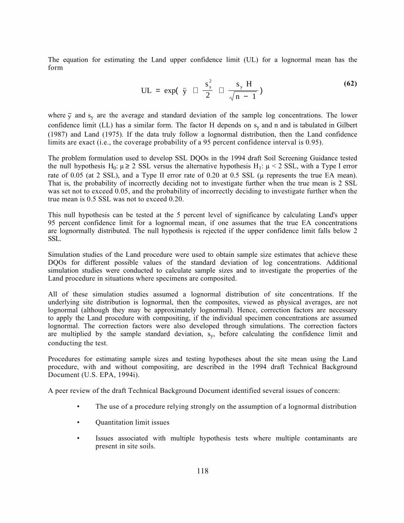
The equation for estimating the Land upper confidence limit (UL) for a lognormal mean has theform
UL = exp( − y + s 2
y
2 +
s y H
n − 1 )
(62)
where − y and sy are the average and standard deviation of the sample log concentrations. The lowerconfidence limit (LL) has a similar form. The factor H depends on sy and n and is tabulated in Gilbert(1987) and Land (1975). If the data truly follow a lognormal distribution, then the Land confidencelimits are exact (i.e., the coverage probability of a 95 percent confidence interval is 0.95).
The problem formulation used to develop SSL DQOs in the 1994 draft Soil Screening Guidance testedthe null hypothesis H0: µ ≥ 2 SSL versus the alternative hypothesis H1: µ < 2 SSL, with a Type I errorrate of 0.05 (at 2 SSL), and a Type II error rate of 0.20 at 0.5 SSL (µ represents the true EA mean).That is, the probability of incorrectly deciding not to investigate further when the true mean is 2 SSLwas set not to exceed 0.05, and the probability of incorrectly deciding to investigate further when thetrue mean is 0.5 SSL was not to exceed 0.20.
This null hypothesis can be tested at the 5 percent level of significance by calculating Land's upper95 percent confidence limit for a lognormal mean, if one assumes that the true EA concentrationsare lognormally distributed. The null hypothesis is rejected if the upper confidence limit falls below 2SSL.
Simulation studies of the Land procedure were used to obtain sample size estimates that achieve theseDQOs for different possible values of the standard deviation of log concentrations. Additionalsimulation studies were conducted to calculate sample sizes and to investigate the properties of theLand procedure in situations where specimens are composited.
All of these simulation studies assumed a lognormal distribution of site concentrations. If theunderlying site distribution is lognormal, then the composites, viewed as physical averages, are notlognormal (although they may be approximately lognormal). Hence, correction factors are necessaryto apply the Land procedure with compositing, if the individual specimen concentrations are assumedlognormal. The correction factors were also developed through simulations. The correction factorsare multiplied by the sample standard deviation, sy, before calculating the confidence limit andconducting the test.
Procedures for estimating sample sizes and testing hypotheses about the site mean using the Landprocedure, with and without compositing, are described in the 1994 draft Technical BackgroundDocument (U.S. EPA, 1994i).
A peer review of the draft Technical Background Document identified several issues of concern:
• The use of a procedure relying strongly on the assumption of a lognormal distribution
• Quantitation limit issues
• Issues associated with multiple hypothesis tests where multiple contaminants arepresent in site soils.
118
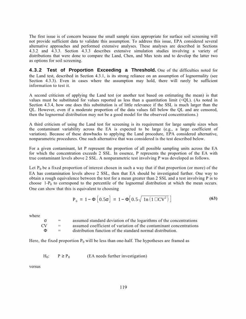
The first issue is of concern because the small sample sizes appropriate for surface soil screening willnot provide sufficient data to validate this assumption. To address this issue, EPA considered severalalternative approaches and performed extensive analyses. These analyses are described in Sections4.3.2 and 4.3.3. Section 4.3.3 describes extensive simulation studies involving a variety ofdistributions that were done to compare the Land, Chen, and Max tests and to develop the latter twoas options for soil screening.
4.3.2 Test of Proportion Exceeding a Threshold. One of the difficulties noted forthe Land test, described in Section 4.3.1, is its strong reliance on an assumption of lognormality (seeSection 4.3.3). Even in cases where the assumption may hold, there will rarely be sufficientinformation to test it.
A second criticism of applying the Land test (or another test based on estimating the mean) is thatvalues must be substituted for values reported as less than a quantitation limit (<QL). (As noted inSection 4.3.4, how one does this substitution is of little relevance if the SSL is much larger than theQL. However, even if a moderate proportion of the data values fall below the QL and are censored,then the lognormal distribution may not be a good model for the observed concentrations.)
A third criticism of using the Land test for screening is its requirement for large sample sizes whenthe contaminant variability across the EA is expected to be large (e.g., a large coefficient ofvariation). Because of these drawbacks to applying the Land procedure, EPA considered alternative,nonparametric procedures. One such alternative that was considered is the test described below.
For a given contaminant, let P represent the proportion of all possible sampling units across the EAfor which the concentration exceeds 2 SSL. In essence, P represents the proportion of the EA withtrue contaminant levels above 2 SSL. A nonparametric test involving P was developed as follows.
Let P0 be a fixed proportion of interest chosen in such a way that if that proportion (or more) of theEA has contamination levels above 2 SSL, then that EA should be investigated further. One way toobtain a rough equivalence between the test for a mean greater than 2 SSL and a test involving P is tochoose 1-P0 to correspond to the percentile of the lognormal distribution at which the mean occurs.One can show that this is equivalent to choosing
P 0 = 1 − Φ 0 . 5 σ = 1 − Φ 0 . 5 1 n 1 + CV2 (63)
whereσ = assumed standard deviation of the logarithms of the concentrations
CV = assumed coefficient of variation of the contaminant concentrationsΦ = distribution function of the standard normal distribution.
Here, the fixed proportion P0 will be less than one-half. The hypotheses are framed as
H0: P ≥ P0 (EA needs further investigation)
versus
119
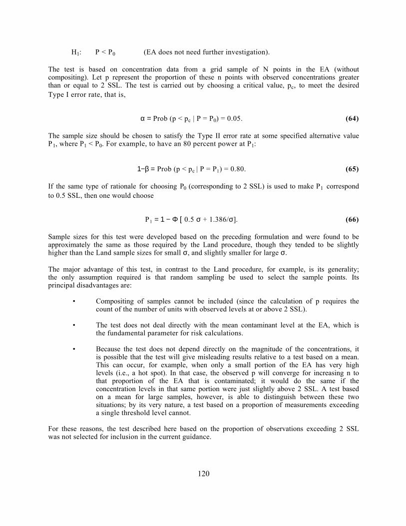
H1: P < P0 (EA does not need further investigation).
The test is based on concentration data from a grid sample of N points in the EA (withoutcompositing). Let p represent the proportion of these n points with observed concentrations greaterthan or equal to 2 SSL. The test is carried out by choosing a critical value, pc, to meet the desiredType I error rate, that is,
α = Prob (p < pc | P = P0) = 0.05. (64)
The sample size should be chosen to satisfy the Type II error rate at some specified alternative valueP1, where P1 < P0. For example, to have an 80 percent power at P1:
1−β = Prob (p < pc | P = P1) = 0.80. (65)
If the same type of rationale for choosing P0 (corresponding to 2 SSL) is used to make P1 correspondto 0.5 SSL, then one would choose
P1 = 1 − Φ [ 0.5 σ + 1.386/σ]. (66)
Sample sizes for this test were developed based on the preceding formulation and were found to beapproximately the same as those required by the Land procedure, though they tended to be slightlyhigher than the Land sample sizes for small σ, and slightly smaller for large σ. The major advantage of this test, in contrast to the Land procedure, for example, is its generality;the only assumption required is that random sampling be used to select the sample points. Itsprincipal disadvantages are:
• Compositing of samples cannot be included (since the calculation of p requires thecount of the number of units with observed levels at or above 2 SSL).
• The test does not deal directly with the mean contaminant level at the EA, which isthe fundamental parameter for risk calculations.
• Because the test does not depend directly on the magnitude of the concentrations, itis possible that the test will give misleading results relative to a test based on a mean.This can occur, for example, when only a small portion of the EA has very highlevels (i.e., a hot spot). In that case, the observed p will converge for increasing n tothat proportion of the EA that is contaminated; it would do the same if theconcentration levels in that same portion were just slightly above 2 SSL. A test basedon a mean for large samples, however, is able to distinguish between these twosituations; by its very nature, a test based on a proportion of measurements exceedinga single threshold level cannot.
For these reasons, the test described here based on the proportion of observations exceeding 2 SSLwas not selected for inclusion in the current guidance.
120
4.3.3 Relative Performance of Land, Max, and Chen Tests. A simulationstudy was conducted to compare the Land, Chen, and Max tests and to determine sample sizesnecessary to achieve DQOs. This section describes the design of the simulation study and summarizesits results. Detailed output from the simulations is presented in Appendix I.
Treatment of Data Below the Quantitation Limit. Review of quantitation limits for110 chemicals showed that for more than 90 percent of the chemicals, the quantitation limit was lessthan 1 percent of the ingestion SSL. In such cases, the treatment of values below the QL is notexpected to have much effect, as long as all data are used in the analysis, with concentrationsassigned to results below the QL in some reasonable way. In the simulations, the QL was assumed tobe SSL/100 and any simulated value below the QL was set equal to 0.5 QL. This is a conservativeassumption based on the comparison of ingestion SSLs with QLs.
Decision Rules. For the Land procedure, as discussed in Section 4.3.1, the null hypothesis H0:µ ≥ 2 SSL (where µ represents the true mean concentration for the EA) can be tested at the 5 percentlevel by calculating Land's upper 95 percent confidence limit for a lognormal mean. The nullhypothesis is rejected (i.e., surface soil contaminant concentrations are less than 2 SSL), if this upperconfidence limit falls below 2 SSL. This application of the Land (1971) procedure, as described in thedraft 1994 Guidance, will be referred to as the "SSL DQOs" and the "original Land procedure."
For the Max test, one decides to walk away if the maximum concentration observed in compositesamples taken from the EA does not exceed 2 SSL. As indicated in Section 4.1.6, it is viewed asproviding a test of the original null hypothesis, H0: µ ≥ 2 SSL. The Max test does not inherentlycontrol either type of error rate (i.e., its critical region is always the region below 2 SSL, not whereconcentrations below a threshold that achieve a specified Type I error rate). However, control oferror rates for the Max test can be achieved through the DQO process by choice of design (i.e., bychoice of the number N of composite samples and choice of the number C of specimens percomposite).
The Chen test requires that the null hypothesis have the form H0: µ ≤ µ 0, with the alternativehypothesis as H1: µ > µ0 (Chen, 1995). Hypotheses or DQOs of this form are referred to as "flippedhypotheses" or "flipped DQOs" because they represent the inverse of the actual hypothesis for SSLdecisions. In the simulations, the Chen method was applied with µ0 = 0.5 SSL at significance levels(Type I error rates) of 0.4, 0.3, 0.2, 0.1, 0.05, 0.025, and 0.01. In this formulation, a Type I erroroccurs if one decides incorrectly to investigate further when the true site mean, µ, is at or below 0.5SSL.
The two formulations of the hypotheses are equivalent in the sense that both allow achievement ofsoil screening DQOs. That is, working with either formulation, it is possible to control theprobability of incorrectly deciding to walk away when the true site mean is 2 SSL and to also controlthe probability of incorrectly deciding to investigate further when the true site mean is 0.5 SSL.
In addition to the original Land procedure, the Chen test, and the Max test, the simulations alsoinclude the Land test of the flipped null hypothesis H0: µ ≤ 0.5 SSL at the 10 percent significancelevel. This Land test of the flipped hypothesis was included to investigate how interchanging the nulland alternative hypotheses affected sample sizes for the Land and Chen procedures.
Simulation Distributions. In the following description of the simulations, parameteracronyms used as labels in the tables of results are indicated by capital letters enclosed in parentheses.
121
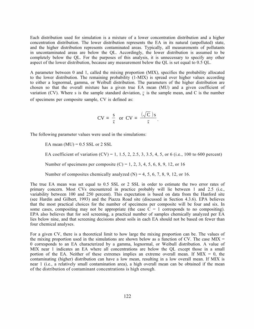
Each distribution used for simulation is a mixture of a lower concentration distribution and a higherconcentration distribution. The lower distribution represents the EA in its natural (unpolluted) state,and the higher distribution represents contaminated areas. Typically, all measurements of pollutantsin uncontaminated areas are below the QL. Accordingly, the lower distribution is assumed to becompletely below the QL. For the purposes of this analysis, it is unnecessary to specify any otheraspect of the lower distribution, because any measurement below the QL is set equal to 0.5 QL.
A parameter between 0 and 1, called the mixing proportion (MIX), specifies the probability allocatedto the lower distribution. The remaining probability (1-MIX) is spread over higher values accordingto either a lognormal, gamma, or Weibull distribution. The parameters of the higher distribution arechosen so that the overall mixture has a given true EA mean (MU) and a given coefficient ofvariation (CV). Where s is the sample standard deviation, − x is the sample mean, and C is the number
of specimens per composite sample, CV is defined as:
CV = s − x
or CV = C s − x
.
The following parameter values were used in the simulations:
EA mean (MU) = 0.5 SSL or 2 SSL
EA coefficient of variation (CV) = 1, 1.5, 2, 2.5, 3, 3.5, 4, 5, or 6 (i.e., 100 to 600 percent)
Number of specimens per composite (C) = 1, 2, 3, 4, 5, 6, 8, 9, 12, or 16
Number of composites chemically analyzed (N) = 4, 5, 6, 7, 8, 9, 12, or 16.
The true EA mean was set equal to 0.5 SSL or 2 SSL in order to estimate the two error rates ofprimary concern. Most CVs encountered in practice probably will lie between 1 and 2.5 (i.e.,variability between 100 and 250 percent). This expectation is based on data from the Hanford site(see Hardin and Gilbert, 1993) and the Piazza Road site (discussed in Section 4.3.6). EPA believesthat the most practical choices for the number of specimens per composite will be four and six. Insome cases, compositing may not be appropriate (the case C = 1 corresponds to no compositing).EPA also believes that for soil screening, a practical number of samples chemically analyzed per EAlies below nine, and that screening decisions about soils in each EA should not be based on fewer thanfour chemical analyses.
For a given CV, there is a theoretical limit to how large the mixing proportion can be. The values ofthe mixing proportion used in the simulations are shown below as a function of CV. The case MIX =0 corresponds to an EA characterized by a gamma, lognormal, or Weibull distribution. A value ofMIX near 1 indicates an EA where all concentrations are below the QL except those in a smallportion of the EA. Neither of these extremes implies an extreme overall mean. If MIX = 0, thecontaminating (higher) distribution can have a low mean, resulting in a low overall mean. If MIX isnear 1 (i.e., a relatively small contamination area), a high overall mean can be obtained if the meanof the distribution of contaminant concentrations is high enough.
122
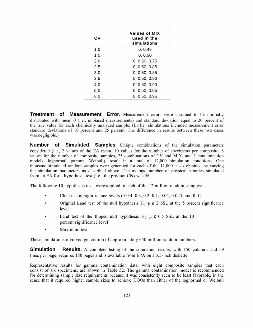
CVValues of MIX
used in thesimulations
1.0 0, 0.491.5 0, 0.502.0 0, 0.50, 0.752.5 0, 0.50, 0.853.0 0, 0.50, 0.853.5 0, 0.50, 0.90
4.0 0, 0.50, 0.905.0 0, 0.50, 0.956.0 0, 0.50, 0.95
Treatment of Measurement Error. Measurement errors were assumed to be normallydistributed with mean 0 (i.e., unbiased measurements) and standard deviation equal to 20 percent ofthe true value for each chemically analyzed sample. (Earlier simulations included measurement errorstandard deviations of 10 percent and 25 percent. The difference in results between these two caseswas negligible.)
Number of Simulated Samples. Unique combinations of the simulation parametersconsidered (i.e., 2 values of the EA mean, 10 values for the number of specimens per composite, 8values for the number of composite samples, 25 combinations of CV and MIX, and 3 contaminationmodels—lognormal, gamma, Weibull), result in a total of 12,000 simulation conditions. Onethousand simulated random samples were generated for each of the 12,000 cases obtained by varyingthe simulation parameters as described above. The average number of physical samples simulatedfrom an EA for a hypothesis test (i.e., the product CN) was 56.
The following 10 hypothesis tests were applied to each of the 12 million random samples:
• Chen test at significance levels of 0.4, 0.3, 0.2, 0.1, 0.05, 0.025, and 0.01
• Original Land test of the null hypothesis H0: µ ≥ 2 SSL at the 5 percent significancelevel
• Land test of the flipped null hypothesis H0: µ ≤ 0.5 SSL at the 10percent significance level
• Maximum test.
These simulations involved generation of approximately 650 million random numbers.
Simulation Results. A complete listing of the simulation results, with 150 columns and 59lines per page, requires 180 pages and is available from EPA on a 3.5-inch diskette.
Representative results for gamma contamination data, with eight composite samples that eachconsist of six specimens, are shown in Table 32. The gamma contamination model is recommendedfor determining sample size requirements because it was consistently seen to be least favorable, in thesense that it required higher sample sizes to achieve DQOs than either of the lognormal or Weibull
123
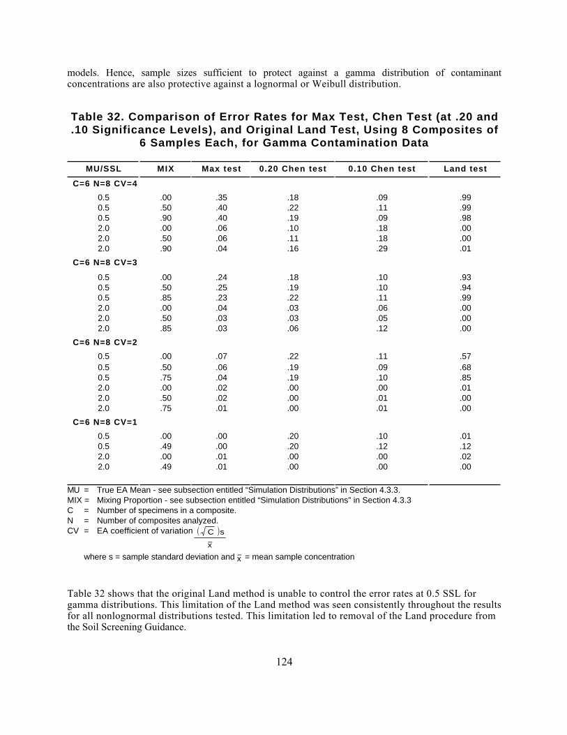
models. Hence, sample sizes sufficient to protect against a gamma distribution of contaminantconcentrations are also protective against a lognormal or Weibull distribution.
Table 32. Comparison of Error Rates for Max Test, Chen Test (at .20 and.10 Significance Levels), and Original Land Test, Using 8 Composites of
6 Samples Each, for Gamma Contamination Data
MU/SSL MIX Max test 0.20 Chen test 0.10 Chen test Land test
C=6 N=8 CV=4
0.50.50.52.02.02.0
.00
.50
.90
.00
.50
.90
.35
.40
.40
.06
.06
.04
.18
.22
.19
.10
.11
.16
.09
.11
.09
.18
.18
.29
.99
.99
.98
.00
.00
.01
C=6 N=8 CV=3
0.50.50.52.02.02.0
.00
.50
.85
.00
.50
.85
.24
.25
.23
.04
.03
.03
.18
.19
.22
.03
.03
.06
.10
.10
.11
.06
.05
.12
.93
.94
.99
.00
.00
.00
C=6 N=8 CV=2
0.50.50.52.02.02.0
.00
.50
.75
.00
.50
.75
.07
.06
.04
.02
.02
.01
.22
.19
.19
.00
.00
.00
.11
.09
.10
.00
.01
.01
.57
.68
.85
.01
.00
.00
C=6 N=8 CV=1
0.50.52.02.0
.00
.49
.00
.49
.00
.00
.01
.01
.20
.20
.00
.00
.10
.12
.00
.00
.01
.12
.02
.00
MU = True EA Mean - see subsection entitled “Simulation Distributions” in Section 4.3.3.MIX = Mixing Proportion - see subsection entitled “Simulation Distributions” in Section 4.3.3C = Number of specimens in a composite.N = Number of composites analyzed.CV = EA coefficient of variation C s
− x
where s = sample standard deviation and − x = mean sample concentration
Table 32 shows that the original Land method is unable to control the error rates at 0.5 SSL forgamma distributions. This limitation of the Land method was seen consistently throughout the resultsfor all nonlognormal distributions tested. This limitation led to removal of the Land procedure fromthe Soil Screening Guidance.
124
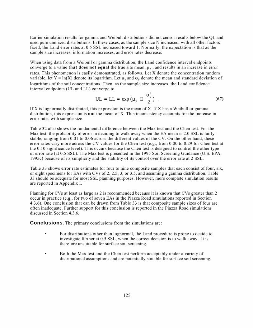
Earlier simulation results for gamma and Weibull distributions did not censor results below the QL andused pure unmixed distributions. In these cases, as the sample size N increased, with all other factorsfixed, the Land error rates at 0.5 SSL increased toward 1. Normally, the expectation is that as thesample size increases, information increases, and error rates decrease.
When using data from a Weibull or gamma distribution, the Land confidence interval endpointsconverge to a value that does not equal the true site mean, µx , and results in an increase in errorrates. This phenomenon is easily demonstrated, as follows. Let X denote the concentration randomvariable, let Y = ln(X) denote its logarithm. Let µy and σy denote the mean and standard deviation oflogarithms of the soil concentrations. Then, as the sample size increases, the Land confidenceinterval endpoints (UL and LL) converge to
UL = LL = exp ( µ y + σ 2
y
2 ) . (67)
If X is lognormally distributed, this expression is the mean of X. If X has a Weibull or gammadistribution, this expression is not the mean of X. This inconsistency accounts for the increase inerror rates with sample size.
Table 32 also shows the fundamental difference between the Max test and the Chen test. For theMax test, the probability of error in deciding to walk away when the EA mean is 2.0 SSL is fairlystable, ranging from 0.01 to 0.06 across the different values of the CV. On the other hand, theseerror rates vary more across the CV values for the Chen test (e.g., from 0.00 to 0.29 for Chen test atthe 0.10 significance level). This occurs because the Chen test is designed to control the other typeof error rate (at 0.5 SSL). The Max test is presented in the 1995 Soil Screening Guidance (U.S. EPA,1995c) because of its simplicity and the stability of its control over the error rate at 2 SSL.
Table 33 shows error rate estimates for four to nine composite samples that each consist of four, six,or eight specimens for EAs with CVs of 2, 2.5, 3, or 3.5, and assuming a gamma distribution. Table33 should be adequate for most SSL planning purposes. However, more complete simulation resultsare reported in Appendix I.
Planning for CVs at least as large as 2 is recommended because it is known that CVs greater than 2occur in practice (e.g., for two of seven EAs in the Piazza Road simulations reported in Section4.3.6). One conclusion that can be drawn from Table 33 is that composite sample sizes of four areoften inadequate. Further support for this conclusion is reported in the Piazza Road simulationsdiscussed in Section 4.3.6.
Conclusions. The primary conclusions from the simulations are:
• For distributions other than lognormal, the Land procedure is prone to decide toinvestigate further at 0.5 SSL, when the correct decision is to walk away. It istherefore unsuitable for surface soil screening.
• Both the Max test and the Chen test perform acceptably under a variety ofdistributional assumptions and are potentially suitable for surface soil screening.
125
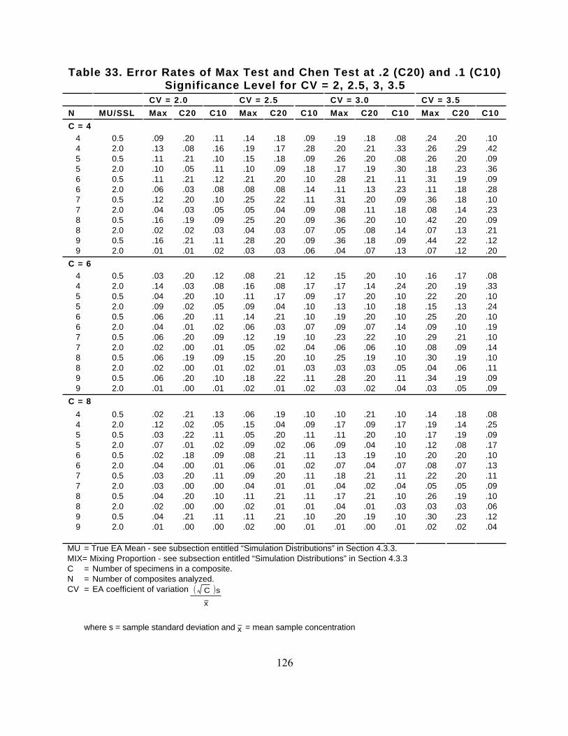
Table 33. Error Rates of Max Test and Chen Test at .2 (C20) and .1 (C10)Significance Level for CV = 2, 2.5, 3, 3.5
CV = 2.0 CV = 2.5 CV = 3.0 CV = 3.5
N MU/SSL Max C20 C10 Max C20 C10 Max C20 C10 Max C20 C10
C = 4445566778899
0.52.00.52.00.52.00.52.00.52.00.52.0
.09
.13
.11
.10
.11
.06
.12
.04
.16
.02
.16
.01
.20
.08
.21
.05
.21
.03
.20
.03
.19
.02
.21
.01
.11
.16
.10
.11
.12
.08
.10
.05
.09
.03
.11
.02
.14
.19
.15
.10
.21
.08
.25
.05
.25
.04
.28
.03
.18
.17
.18
.09
.20
.08
.22
.04
.20
.03
.20
.03
.09
.28
.09
.18
.10
.14
.11
.09
.09
.07
.09
.06
.19
.20
.26
.17
.28
.11
.31
.08
.36
.05
.36
.04
.18
.21
.20
.19
.21
.13
.20
.11
.20
.08
.18
.07
.08
.33
.08
.30
.11
.23
.09
.18
.10
.14
.09
.13
.24
.26
.26
.18
.31
.11
.36
.08
.42
.07
.44
.07
.20
.29
.20
.23
.19
.18
.18
.14
.20
.13
.22
.12
.10
.42
.09
.36
.09
.28
.10
.23
.09
.21
.12
.20
C = 6445566778899
0.52.00.52.00.52.00.52.00.52.00.52.0
.03
.14
.04
.09
.06
.04
.06
.02
.06
.02
.06
.01
.20
.03
.20
.02
.20
.01
.20
.00
.19
.00
.20
.00
.12
.08
.10
.05
.11
.02
.09
.01
.09
.01
.10
.01
.08
.16
.11
.09
.14
.06
.12
.05
.15
.02
.18
.02
.21
.08
.17
.04
.21
.03
.19
.02
.20
.01
.22
.01
.12
.17
.09
.10
.10
.07
.10
.04
.10
.03
.11
.02
.15
.17
.17
.13
.19
.09
.23
.06
.25
.03
.28
.03
.20
.14
.20
.10
.20
.07
.22
.06
.19
.03
.20
.02
.10
.24
.10
.18
.10
.14
.10
.10
.10
.05
.11
.04
.16
.20
.22
.15
.25
.09
.29
.08
.30
.04
.34
.03
.17
.19
.20
.13
.20
.10
.21
.09
.19
.06
.19
.05
.08
.33
.10
.24
.10
.19
.10
.14
.10
.11
.09
.09
C = 8
445566778899
0.52.00.52.00.52.00.52.00.52.00.52.0
.02
.12
.03
.07
.02
.04
.03
.03
.04
.02
.04
.01
.21
.02
.22
.01
.18
.00
.20
.00
.20
.00
.21
.00
.13
.05
.11
.02
.09
.01
.11
.00
.10
.00
.11
.00
.06
.15
.05
.09
.08
.06
.09
.04
.11
.02
.11
.02
.19
.04
.20
.02
.21
.01
.20
.01
.21
.01
.21
.00
.10
.09
.11
.06
.11
.02
.11
.01
.11
.01
.10
.01
.10
.17
.11
.09
.13
.07
.18
.04
.17
.04
.20
.01
.21
.09
.20
.04
.19
.04
.21
.02
.21
.01
.19
.00
.10
.17
.10
.10
.10
.07
.11
.04
.10
.03
.10
.01
.14
.19
.17
.12
.20
.08
.22
.05
.26
.03
.30
.02
.18
.14
.19
.08
.20
.07
.20
.05
.19
.03
.23
.02
.08
.25
.09
.17
.10
.13
.11
.09
.10
.06
.12
.04
MU = True EA Mean - see subsection entitled “Simulation Distributions” in Section 4.3.3.MIX= Mixing Proportion - see subsection entitled “Simulation Distributions” in Section 4.3.3 C = Number of specimens in a composite.N = Number of composites analyzed.CV = EA coefficient of variation C s
− x
where s = sample standard deviation and − x = mean sample concentration
126
4.3.4 Treatment of Observations Below the Limit of Quantitation. Testprocedures that are based on estimating a mean contaminant level for an EA, such as the Land andChen procedures, make use of each measured concentration value. For this reason, the use of allreported concentration measurements in such calculations should be considered regardless of theirmagnitude—that is, even if the measured levels fall below a quantitation level. One argument for thisapproach is that the QL is itself an estimate. Another is that some value will have to be substitutedfor any censored data point (i.e., a point reported as <QL), and the actual measured value is at leastas accurate as a substituted value.
The peer review of the Draft Soil Screening Guidance raised the following issue:
If such censored values do occur in a data set, what values should be used?
There is a substantial amount of literature on this subject and a variety of sophisticated approaches.In the context of SSLs, however, a simple approach is recommended. Consistent with generalSuperfund guidance, each observation reported as "<QL" shall be replaced with 0.5 QL forcomputation of the sample mean.
The evidence suggests that the ingestion SSL generally will be 2 orders of magnitude or more greaterthan the QL for most contaminants. In these cases, the results of soil screening will be insensitive toalternative procedures that could be used to substitute values for observations reported as "<QL."When the SSL is not much greater than the QL (e.g., SSL < 50 QL), the outcome of the soilscreening could be affected by the procedure used to substitute for "<QL" values.
The most conservative approach would be to substitute the concentration represented by the QLitself for all observations reported as "<QL." In the context of the SSLs, however, the simpleapproach of using 0.5 QL is suggested. This will be sufficiently conservative given the conservativefactors underlying the SSLs.
4.3.5 Multiple Hypothesis Testing Considerations. The Soil Screening Guidanceaddresses the following hypothesis testing problem for each EA:
H0: mean concentration of a given chemical ≥ 2 SSL versus
H1: mean concentration of a given chemical < 2 SSL.
The default value for the probability of a Type I error is α = 0.05, while the default value for thepower of the test at 0.5 SSL is 1-ß = 0.80. The test is applied separately for each chemical, so thatthese probabilities apply for each individual chemical. Thus, there is an 80 percent probability ofwalking away from an EA (i.e., rejecting H0) when only one chemical is being tested and its truemean level is 0.5 SSL and a 5 percent probability of walking away if its true mean level is 2 SSL.
However, the Soil Screening Guidance does not explicitly address the following issues:
What is the composite probability of walking away from an EA if there aremultiple contaminants?
andIf such probabilities are unacceptable, how should one compensate when testingfor multiple contaminants within a single EA?
127
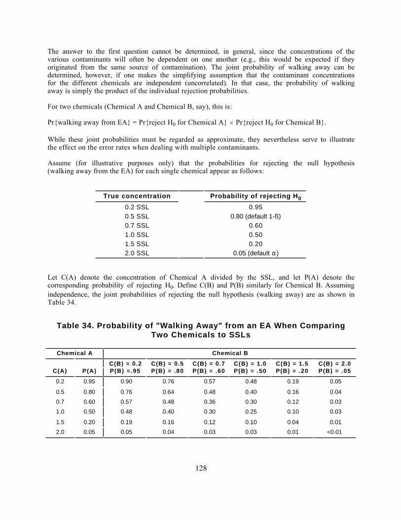
The answer to the first question cannot be determined, in general, since the concentrations of thevarious contaminants will often be dependent on one another (e.g., this would be expected if theyoriginated from the same source of contamination). The joint probability of walking away can bedetermined, however, if one makes the simplifying assumption that the contaminant concentrationsfor the different chemicals are independent (uncorrelated). In that case, the probability of walkingaway is simply the product of the individual rejection probabilities.
For two chemicals (Chemical A and Chemical B, say), this is:
Pr{walking away from EA} = Pr{reject H0 for Chemical A} H Pr{reject H0 for Chemical B}.
While these joint probabilities must be regarded as approximate, they nevertheless serve to illustratethe effect on the error rates when dealing with multiple contaminants.
Assume (for illustrative purposes only) that the probabilities for rejecting the null hypothesis(walking away from the EA) for each single chemical appear as follows:
True concentration Probability of rejecting H0
0.2 SSL 0.950.5 SSL 0.80 (default 1-ß)0.7 SSL 0.601.0 SSL 0.501.5 SSL 0.202.0 SSL 0.05 (default α)
Let C(A) denote the concentration of Chemical A divided by the SSL, and let P(A) denote thecorresponding probability of rejecting H0. Define C(B) and P(B) similarly for Chemical B. Assumingindependence, the joint probabilities of rejecting the null hypothesis (walking away) are as shown inTable 34.
Table 34. Probability of "Walking Away" from an EA When ComparingTwo Chemicals to SSLs
Chemical A Chemical B
C(A) P(A)C(B) = 0.2P(B) =.95
C(B) = 0.5P(B) = .80
C(B) = 0.7P(B) = .60
C(B) = 1.0P(B) = .50
C(B) = 1.5P(B) = .20
C(B) = 2.0P(B) = .05
0.2 0.95 0.90 0.76 0.57 0.48 0.19 0.05
0.5 0.80 0.76 0.64 0.48 0.40 0.16 0.04
0.7 0.60 0.57 0.48 0.36 0.30 0.12 0.03
1.0 0.50 0.48 0.40 0.30 0.25 0.10 0.03
1.5 0.20 0.19 0.16 0.12 0.10 0.04 0.01
2.0 0.05 0.05 0.04 0.03 0.03 0.01 <0.01
128
These probabilities demonstrate that the test procedure will tend to be very conservative if multiplechemicals are involved—that is, all of the chemical concentrations must be quite low relative totheir SSL in order to have a high probability of walking away from the EA. On the other hand, therewill be a high probability that further investigation will be called for if the mean concentration foreven a single chemical is twice the SSL.
A potential problem occurs when there are several chemicals under consideration and when all ormost of them have levels slightly below the SSL (e.g., near 0.5 SSL). For instance, if each of sixindependent chemicals had levels at 0.5 SSL, the probability of rejecting the null hypothesis would be80 percent for each such chemical, but the probability of walking away from the EA would be only(0.80)6 = 0.26.
If the same samples are being analyzed for multiple chemicals, then the original choice for thenumber of such samples ideally should have been based on the worst case (i.e., the chemical expectedto have the largest variability). In this case, the probability of correctly rejecting the null hypothesisat 0.5 SSL for the chemicals with less variability will be higher. The overall probability of walkingaway will be greater than shown above if all or some of the chemicals have less variability thanassumed as the basis for determining sample sizes. Here, the sample size will be large enough for theprobability of rejecting the null hypothesis at 0.5 SSL to be greater than 0.80 for these chemicals.
The probability values assumed above for deciding that no further investigation is necessary forindividual chemicals, which are the basis for these conclusions, are equally applicable for the Land,Chen, and Max tests. They simply represent six hypothetical points of the power curves for thesetests (from 0.2 SSL to 2.0 SSL). Therefore, the conclusions are equally applicable for each of thehypothesis testing procedures that have been considered in the current guidance for screening surfacesoils.
If the surface soil concentrations are positively correlated, as expected when dealing with multiplechemicals, then it is likely that either all the chemicals of concern have relatively highconcentrations or they all have relatively low concentrations. In this case, the probability of makingthe correct decision for an EA would be greater than that suggested by the above calculations thatassume independence of the various chemicals.
However, the potential problem of several chemicals having concentrations near 0.5 SSL is notprecluded by assuming positive correlations. In fact, it suggests that if the EA average for onechemical is near 0.5 SSL, then the average for others is also likely to be near 0.5 SSL, which isexactly the situation where the probability of not walking away from the EA can become largebecause there is a high probability that H0 will be rejected for at least one of these chemicals.
An alternative would be to use multiple hypothesis testing procedures to control the overall errorrate for the set of chemicals (i.e., the set of hypothesis tests) rather than the separate error rates forthe individual chemicals. Guidance for performing multiple hypothesis tests is beyond the scope ofthe current document. Obtain the advice of a statistician familiar with multiple hypothesis testingprocedures if the overall error rates for multiple chemicals is of concern for a particular site. Theclassical statistical guidance regarding this subject is Simultaneous Statistical Inference (Miller, 1991).
4.3.6 Investigation of Compositing Within EA Sectors. If one decides that anEA needs further investigation, then it is natural to inquire which portion(s) of the EA exceed thescreening level. This is a different question than simply asking whether or not the EA average soilconcentration exceeds the SSL. Conceivably, this question may require additional sampling, chemical
129
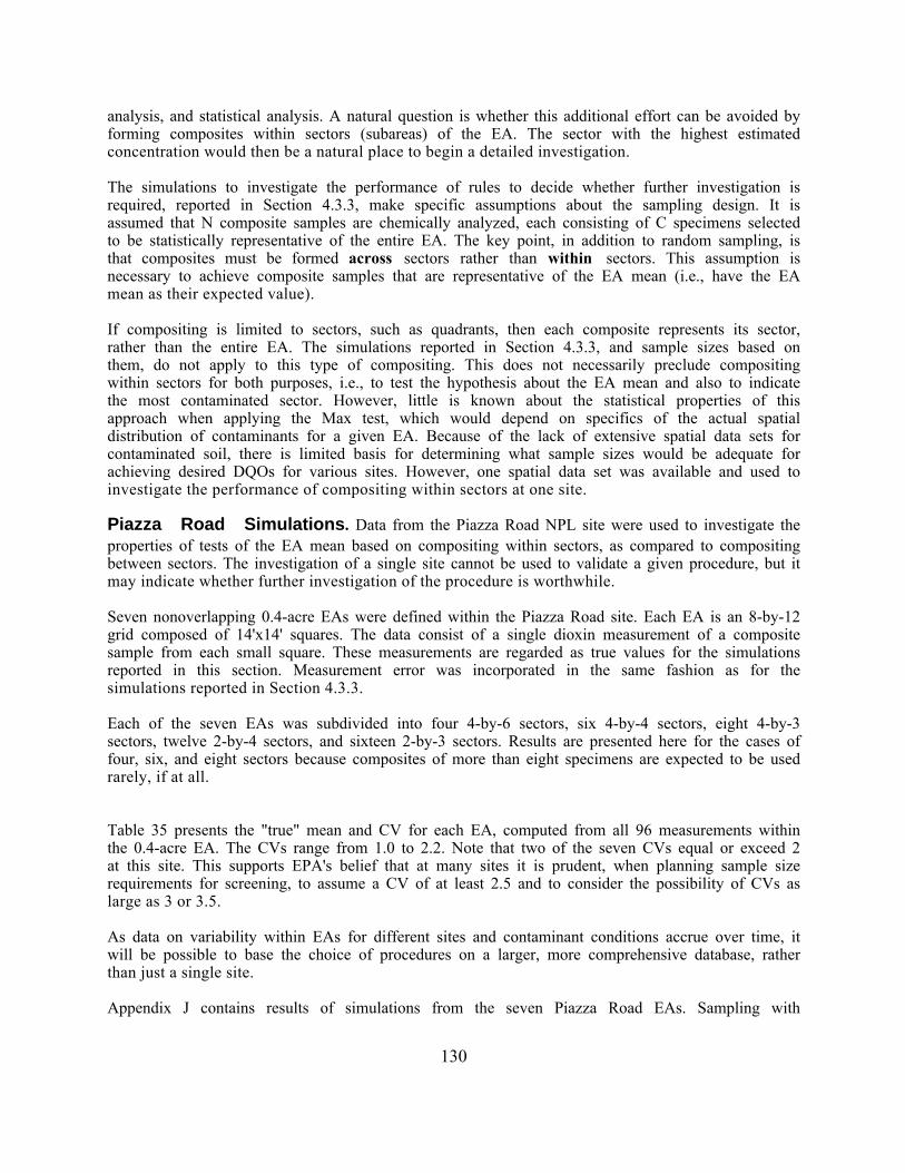
analysis, and statistical analysis. A natural question is whether this additional effort can be avoided byforming composites within sectors (subareas) of the EA. The sector with the highest estimatedconcentration would then be a natural place to begin a detailed investigation.
The simulations to investigate the performance of rules to decide whether further investigation isrequired, reported in Section 4.3.3, make specific assumptions about the sampling design. It isassumed that N composite samples are chemically analyzed, each consisting of C specimens selectedto be statistically representative of the entire EA. The key point, in addition to random sampling, isthat composites must be formed across sectors rather than within sectors. This assumption isnecessary to achieve composite samples that are representative of the EA mean (i.e., have the EAmean as their expected value).
If compositing is limited to sectors, such as quadrants, then each composite represents its sector,rather than the entire EA. The simulations reported in Section 4.3.3, and sample sizes based onthem, do not apply to this type of compositing. This does not necessarily preclude compositingwithin sectors for both purposes, i.e., to test the hypothesis about the EA mean and also to indicatethe most contaminated sector. However, little is known about the statistical properties of thisapproach when applying the Max test, which would depend on specifics of the actual spatialdistribution of contaminants for a given EA. Because of the lack of extensive spatial data sets forcontaminated soil, there is limited basis for determining what sample sizes would be adequate forachieving desired DQOs for various sites. However, one spatial data set was available and used toinvestigate the performance of compositing within sectors at one site.
Piazza Road Simulations. Data from the Piazza Road NPL site were used to investigate theproperties of tests of the EA mean based on compositing within sectors, as compared to compositingbetween sectors. The investigation of a single site cannot be used to validate a given procedure, but itmay indicate whether further investigation of the procedure is worthwhile.
Seven nonoverlapping 0.4-acre EAs were defined within the Piazza Road site. Each EA is an 8-by-12grid composed of 14'x14' squares. The data consist of a single dioxin measurement of a compositesample from each small square. These measurements are regarded as true values for the simulationsreported in this section. Measurement error was incorporated in the same fashion as for thesimulations reported in Section 4.3.3.
Each of the seven EAs was subdivided into four 4-by-6 sectors, six 4-by-4 sectors, eight 4-by-3sectors, twelve 2-by-4 sectors, and sixteen 2-by-3 sectors. Results are presented here for the cases offour, six, and eight sectors because composites of more than eight specimens are expected to be usedrarely, if at all.
Table 35 presents the "true" mean and CV for each EA, computed from all 96 measurements withinthe 0.4-acre EA. The CVs range from 1.0 to 2.2. Note that two of the seven CVs equal or exceed 2at this site. This supports EPA's belief that at many sites it is prudent, when planning sample sizerequirements for screening, to assume a CV of at least 2.5 and to consider the possibility of CVs aslarge as 3 or 3.5.
As data on variability within EAs for different sites and contaminant conditions accrue over time, itwill be possible to base the choice of procedures on a larger, more comprehensive database, ratherthan just a single site.
Appendix J contains results of simulations from the seven Piazza Road EAs. Sampling with
130
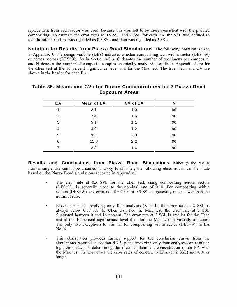
replacement from each sector was used, because this was felt to be more consistent with the plannedcompositing. To estimate the error rates at 0.5 SSL and 2 SSL for each EA, the SSL was defined sothat the site mean first was regarded as 0.5 SSL and then was regarded as 2 SSL.
Notation for Results from Piazza Road Simulations. The following notation is usedin Appendix J. The design variable (DES) indicates whether compositing was within sector (DES=W)or across sectors (DES=X). As in Section 4.3.3, C denotes the number of specimens per composite,and N denotes the number of composite samples chemically analyzed. Results in Appendix J are forthe Chen test at the 10 percent significance level and for the Max test. The true mean and CV areshown in the header for each EA.
Table 35. Means and CVs for Dioxin Concentrations for 7 Piazza RoadExposure Areas
EA Mean of EA CV of EA N
1 2.1 1.0 96
2 2.4 1.6 96
3 5.1 1.1 96
4 4.0 1.2 96
5 9.3 2.0 96
6 15.8 2.2 96
7 2.8 1.4 96
Results and Conclusions from Piazza Road Simulations. Although the resultsfrom a single site cannot be assumed to apply to all sites, the following observations can be madebased on the Piazza Road simulations reported in Appendix J.
• The error rate at 0.5 SSL for the Chen test, using compositing across sectors(DES=X), is generally close to the nominal rate of 0.10. For compositing withinsectors (DES=W), the error rate for Chen at 0.5 SSL is generally much lower than thenominal rate.
• Except for plans involving only four analyses (N = 4), the error rate at 2 SSL isalways below 0.05 for the Chen test. For the Max test, the error rate at 2 SSLfluctuated between 0 and 16 percent. The error rate at 2 SSL is smaller for the Chentest at the 10 percent significance level than for the Max test in virtually all cases.The only two exceptions to this are for compositing within sector (DES=W) in EANo. 6.
• This observation provides further support for the conclusion drawn from thesimulations reported in Section 4.3.3: plans involving only four analyses can result inhigh error rates in determining the mean contaminant concentration of an EA withthe Max test. In most cases the error rates of concern to EPA (at 2 SSL) are 0.10 orlarger.
131

• In general, error rates estimated from Piazza Road simulations for compositing acrosssectors are at least as small as would be predicted on the basis of the simulation resultsreported in Section 4.3.3.
• The simulation results show that compositing within sectors using the Max test maybe an option for site managers who want to know whether one sector of an EA ismore contaminated than the other. However, use of the Max test when compositingwithin sectors may lead the site manager to draw conclusions about the meancontaminant concentration in that sector only, not across the entire EA.
132