Parametric Tolerance Analysis of Mechanical Assembly …file.scirp.org/pdf/ICA20100100001_51724716.pdf · Parametric Tolerance Analysis of Mechanical Assembly by ... balance manufacturing

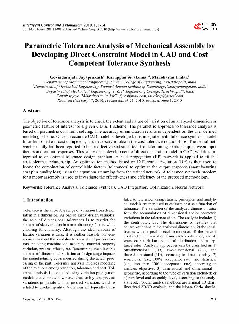
Intelligent Control and Automation, 2010, 1, 1-14 doi:10.4236/ica.201.11001 Published Online August 2010 (http://www.SciRP.org/journal/ica)

Copyright © 2010 SciRes. ICA

Parametric Tolerance Analysis of Mechanical Assembly by Developing Direct Constraint Model in CAD and Cost

Competent Tolerance Synthesis

Govindarajalu Jayaprakash1, Karuppan Sivakumar2, Manoharan Thilak3 1Department of Mechanical Engineering, Shivani College of Engineering, Tiruchirapalli, India

2Department of Mechanical Engineering, Bannari Amman Institute of Technology, Sathiyamangalam, India 3Department of Mechanical Engineering, T. R. P. Engineering College, Tiruchirapalli, India

E-mail: [email protected], [email protected], [email protected] Received February 17, 2010; revised March 21, 2010; accepted June 1, 2010

Abstract The objective of tolerance analysis is to check the extent and nature of variation of an analyzed dimension or geometric feature of interest for a given GD & T scheme. The parametric approach to tolerance analysis is based on parametric constraint solving. The accuracy of simulation results is dependent on the user-defined modeling scheme. Once an accurate CAD model is developed, it is integrated with tolerance synthesis model. In order to make it cost competent, it is necessary to obtain the cost-tolerance relationships. The neural net-work recently has been reported to be an effective statistical tool for determining relationship between input factors and output responses. This study deals development of direct constraint model in CAD, which is in-tegrated to an optimal tolerance design problem. A back-propagation (BP) network is applied to fit the cost-tolerance relationship. An optimization method based on Differential Evolution (DE) is then used to locate the combination of controllable factors (tolerances) to optimize the output response (manufacturing cost plus quality loss) using the equations stemming from the trained network. A tolerance synthesis problem for a motor assembly is used to investigate the effectiveness and efficiency of the proposed methodology. Keywords: Tolerance Analysis, Tolerance Synthesis, CAD Integration, Optimization, Neural Network

1. Introduction Tolerance is the allowable range of variation from design intent in a dimension. As one of many design variables, the role of dimensional tolerances is to restrict the amount of size variation in a manufacturing feature while ensuring functionality. Although the ideal amount of feature variation is zero, it is neither feasible nor eco-nomical to meet the ideal due to a variety of process fac-tors including machine tool accuracy, material property variation, process effects, etc. Determining the allowable amount of dimensional variation at design stage impacts the manufacturing costs incurred during the actual proc-essing of the part. Tolerance analysis involves modeling of the relations among variation, tolerance and cost. Tol-erance analysis is conducted using variation propagation models that compute how part, subassembly, and process variations propagate to final product variation, which is related to product quality. Variations are typically trans-

lated to tolerances using statistic principles, and analyti-cal models are then used to estimate cost as a function of tolerance. The variation of the analyzed dimension arise form the accumulation of dimensional and/or geometric variations in the tolerance chain. The analysis include: 1) the contributor, i.e., The dimensions or features that causes variations in the analyzed dimension, 2) the sensi-tivities with respect to each contributor, 3) the percent contribution to variation from each contributor, and 4) worst case variations, statistical distribution, and accep-tance rates. Analysis approaches can be classified as 1) one-dimensional (1D), two-dimensional (2D), and three-dimensional (3D), according to dimensionality; 2) worst case (i.e., 100% acceptance rate) and statistical (i.e., less than 100% acceptance rate), according to analysis objective; 3) dimensional and dimensional + geometric, according to the type of variation included; or 4) part level and assembly level, according to the analy-sis level. Popular analysis methods are manual 1D chart, linearized 2D/3D analysis, and the Monte Carlo simula-

G. JAYAPRAKASH ET AL.


2

tion. At the present time, three different and disconnected

communities i.e., designers/draftsmen, engineering ana-lysts, and design researchers are using vastly different tools and techniques for tolerance analysis. Cultural and educational differences between these communities have isolated them from one another and made them unaware of the others’ techniques. The draftsmen community uses a manual procedure called tolerance charts; but can do only worst-case analysis, and is conducted in only one direction at a time. Meanwhile, the engineering analysis community uses computer-aided tolerancing software CATs. These CAT packages can do both worst-case and statistical analyses. Many researchers [1-4] provided good surveys of GD&T modeling for CATs; Some re-searcher [5] discussed the simplification of feature based models for tolerance analysis, and used the linear pro-gramming approach to tolerance analysis involving geo-metric tolerances [5]; Guilford et al. [2] introduced a CAT system using the variation modeling and feasibility space approaches. 2. Background 2.1. 1D Tolerance Charts Tolerance charting is a manual bookkeeping procedure for 1D stack calculations. The analyst typically works with engineering drawings [6-7]. Since the method is limited to worst-case analysis, the analyst positions parts in assemblies to yield each of the worst-cases minimum or maximum value of the analyzed dimension, i.e., sepa-rate charts have to be constructed for each worst-case. Since no algebraic expression for the analyzed dimension in terms of the contributors is generated by this method, no statistical analysis can be performed. Also, contribu-tors not in the direction of analysis are ignored, which may yield significant errors in most cases. The limita-tions associated with this method, as practiced today, are as follows. 1) It is done manually, and since each type of tolerance is handled differently, the user must remember all the rules correctly while constructing the charts to obtain correct results, making the process tedious and prone to errors. 2) It deals with one direction at a time, ignoring possible contributions from other directions, which often leads to inaccurate results. 3) The charting procedure is only capable of the worst-case analysis only; no statistical analysis is available. 4). This method has not been widely integrated with existing CAD systems. 2.2. Parametric Tolerance Analysis Most CAT packages take advantage of the same para-metric/variational approach used in CAD systems and

apply the Monte Carlo simulation to tolerance analysis [8-10]. This section will give a brief description of pa-rametric approach to tolerance analysis. In the parametric approach, the analyzed dimension is expressed as an al-gebraic function an equation, or a set of equations that relates the analyzed dimension to those on which it de-pends i.e., contributors. The function is either linearized or directly used for the Monte Carlo simulation in the nonlinear analysis. Results commonly available are the lists of contributors, sensitivities, and percentage contri-butions, and the tolerance accumulation for worst-case and statistical cases. 2.3. Cost Competent Tolerancing Aspects such as design for quality, quality improvement and cost reduction, asymmetric quality losses, charts for optimum quality and cost, minimum cost approach, cost of assemblies, development of cost tolerance models [11-15] have been explored in the quality area of toler-ance synthesis. Experiments (DOE) approach was used in robust tolerance design, the cases of ‘nominal the best’, ‘smaller the better’, ‘larger the better’, and asymmetric loss function, were investigated [16] and allocation of tolerances of products with asymmetric quality loss was presented [14]. The combined effect of manufacturing cost and quality loss was also investigated under the re-straints of process capability limits, design functionality restriction and product quality requirements by using tolerance chart optimization for quality and cost [12]. Relationships between the product cost and tolerances have also been investigated. An analytical method was proposed for determining tolerances for mechanical parts with objectives of minimizing manufacturing costs [17]. Minimizing the cost of assembly was investigated mathematically in which it was observed that widening the tolerance of more expensive part and a tightening of tolerances on cheaper parts could result in major reduc-tion in cost of the assembly [18]. Exhaustive search, zero–one, SQP and Univariate methods were evaluated for performing a combined minimum cost tolerance al-location and process selection [19]. The production cost tolerance and hybrid tolerance models based on empiri-cal cost tolerance data of manufacturing processes like punching, turning, milling, grinding and casting were introduced [20]. The robust design by tolerance alloca-tion considering quality and manufacturing cost and op-timizing tolerance allocation based on manufacturing cost were also investigated [21,22]. It involved develop-ment of relationship between part tolerances and assem-bly tolerances to provide a quantitative measure of prod-uct quality using the quality loss function concept intro-duced by Taguchi. Numerical optimization was used to balance manufacturing cost and product quality. The possibility of using statistics and probability methods for



3

allocation of tolerances has also been explored with a view to developing tools for tolerance synthesis.

Relationship between function and dimensional varia-tion on assembly was considered as logical basis for se-lection of tolerances [23]. A probabilistic model for tol-erance synthesis was developed [24] in which the reli-ability indices were associated with either assembly con-dition or component dimension. Strategies to compute small changes or gradient in tolerance values were also developed using probability theory [25]. Tolerance cost models based on the distribution function zone [26], tol-erance optimization problem using system of experi-mental design [27] and using Monte–Carlo simulations [28] approaches, were also investigated in application of statistical methods for tolerance synthesis. 2.4. Neural Network-Based Cost-Tolerance

Functions Neural networks have received a lot of attention in many research and application areas. One of the major benefits of neural networks is the adaptive ability of their gener-alization of data from the real world. Exploiting this ad-vantage, many researchers apply neural networks for nonlinear regression analysis and have reported positive experimental results in their applications [29]. Recently, neural networks have received a great deal of attention in manufacturing areas. Zhang and Huang [30] presented an extensive review of neural network applications in manufacturing. Neural networks are defined by Rumel-hart and McClelland [31] as `massively parallel inter-connected networks of simple (usually adaptive) ele-ments and their hierarchical organizations which are in-tended to interact with objects of the real world in the same way as biological nervous systems do. The ap-proach towards constructing the cost} tolerance rela-tionships is based on a supervised back-propagation (BP) neural network. Among several well-known supervised neural networks, the BP model is the most extensively used and can provide good solutions for much industrial application [32].

A BP network is a feed-forward network with one or more layers of nodes between the input and output nodes. An imperative item of the BP network is the iterative method that propagates the error terms required to adopt weights back from nodes in the output layer to nodes in lower layers. The training of a BP network involves three stages: the feed forward of the input training pattern, the calculation and BP of the associated error, and the ad-justment of the weights. After the network reaches a sat-isfactory level of performance, it will learn the relation-ships between input and output patterns and its weights can be used to recognize new input patterns.

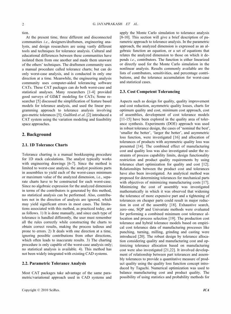
Figure 1 depicts a BP network with one hidden layer. The hidden nodes of the hidden layer perform an impor-

Figure 1. Architecture of a three-layer BP network. tant role in creating internal representation. The follow-ing nomenclatures are used for describing the BP learn-ing rule.

netpi = net input to processing unit i in pattern p (a pat-tern corresponding to a vector of factors),

wij = connection weight between processing unit I and processing unit j,

api = activation value of processing unit i in pattern p, pi = the effect of a change on the output of unit I in

pattern p, gpi = target value of processing unit i, = learning rate. The net inputs and the activation values of the middle

processing nodes are calculated as follows:

pi ij pjj

net w a (1)

pi

pi

1a

1 exp net

(2)

The net input is the weighed sum of activation values of the connected input units plus a bias value. Initially, the connection weights are assigned randomly and are varied continuously. The activation values are in turn used to calculate the net inputs and the activation values of the output processing units using the same Equations (1) and (2).

Once the activation values of the output units are cal-culated, we compare the target value with activation value of each output unit. The discrepancy is propagated using.

'pi pi pi i piδ g a f net (3)

For the hidden processing units in which the target values are unknown, instead of Equation (3), the follow-ing equation is used to calculate the discrepancy. It takes the form

'pi i pi pk ki

k

δ f net δ w (4)

From the results of Equations (3) and (4), the weights between processing units are adjusted using

ij pi pjw εδ a (5)



4

2.5. Differential Evolution (DE) Differential Evolution is an improved version of Genetic Algorithm for faster optimization [33]. Unlike simple GA that uses binary coding for representing problem parameters, Differential Evolution (DE) uses real coding of floating point numbers. Among the DE’s advantages are its simple structure, ease of use, speed and robust-ness. The simple adaptive scheme used by DE ensures that the mutation increments are automatically scaled to the cor-rect magnitude. Similarly DE uses a non-uniform cross-over in that the parameter values of the child vector are inherited in unequal proportions from the parent vectors. For reproduction, DE uses a tournament selection where the child vector competes against one of its parents. The overall structure of the DE algorithm resembles that of most other population based searches. The parallel ver-sion of DE maintains two arrays, each of which holds a population of NP, D-dimensional, real valued vectors. The primary array holds the current vector population, while the secondary array accumulates vectors that are selected for the next generation. In each generation, NP competitions are held to determine the composition of the next generation. Every pair of vectors (Xa, Xb) de-fines a vector differential: Xa – Xb. When Xa and Xb are chosen randomly, their weighted differential is used to perturb another randomly chosen vector Xc. This process can be mathematically written as X’c = Xc + F (Xa – Xb). The scaling factor F is a user supplied constant in the range (0 < F < 1.2). The optimal value of F for most of the functions lies in the range of 0.4 to 1.0 [33]. Then in every generation, each primary array vector, Xi is tar-geted for crossover with a vector like X’c to produce a trial vector Xt. Thus the trial vector is the child of two parents, a noisy random vector and the target vector against which it must compete. The non-uniform cross-over is used with a crossover constant CR, in the range 0 < CR < 1. CR actually represents the probability that the child vector inherits the parameter values from the noisy random vector. When CR = 1, for example, every trial vector parameter is certain to come from X’c. If, on the other hand, CR = 0, all but one trial vector parameter comes from the target vector. To ensure that Xt differs from Xi by at least one parameter, the final trial vector parameter always comes from the noisy random vector, even when CR = 0. Then the cost of the trial vector is compared with that of the target vector, and the vector that has the lowest cost of the two would survive for the next generation. In all, just three factors control evolu-tion under DE, the population size, NP; the weight ap-plied to the random differential, F; and the crossover constant, CR.

The general convention used is DE/x/y/z. DE stands for Differential Evolution, x represents a string denoting

the vector to be perturbed, y is the number of difference vectors considered for perturbation of x, and z stands for the type of crossover being used (exp:exponential; bin: binomial). Thus, the working algorithm outlined above is the strategy of DE, i.e..DE/rand/1/bin. Hence the pertur-bation can be either in the best vector of the previous generation or in any randomly chosen vector. Similarly for perturbation either single or two vector differences can be used. For perturbation with a single vector differ-ence, out of the three distinct randomly chosen vectors, the weighted vector differential of any two vectors is added to the third one. Similarly for perturbation with two vector differences, five distinct vectors, other than the target vector are chosen randomly from the current popu-lation. Out of these, the weighted vector difference of each pair of any four vectors is added to the fifth one for per-turbation. In binomial crossover, the crossover is per-formed on each of the D variables whenever a randomly picked number between 0 and 1 is within the CR value. 2.5.1. Pseudo Code for DE The pseudo code of DE used in the present study is given below: · Choose a seed for the random number generator. · Initialize the values of D, NP, CR, F and MAXGEN (maximum generation). · Initialize all the vectors of the population randomly. The variables are normalized within the bounds. Hence generate a random number between 0 and 1 for all the design variables for initialization. for i = 1 to NP { for j = 1 to D Xi, j = Lower bound + random number *( upper bound - lower bound)} · All the vectors generated should satisfy the constraints. Penalty function approach, i.e., penalizing the vector by giving it a large value, is followed only for those vectors, which do not satisfy the constraints. · Evaluate the objective function of each vector. Here is the value of the objective function to be minimized cal-culated by a separate function defunct. objective () for i = 1 to NP Ci = defunct. objective () · Find out the vector with the minimum objective value i.e. the best vector so far. Cmin = C1 and best = 1 for i = 2 to NP { if (Ci < Cmin) then Cmin = Ci and best = i } · Perform mutation, crossover, selection and evaluation of the objective function for a specified number of generations. While (gen < MAXGEN) { for i = 1 to NP { · For each vector Xi (target vector), select three distinct



5

vectors Xa, Xb and Xc (select five, if two vector differ-ences are to be used) randomly from the current popula-tion (primary array) other than the vector Xi do { r1 = random number * NP r2 = random number * NP r3 = random number * NP } while (r1 = i) OR (r2 = i) OR (r3 = i) OR (r1 = r2) OR (r2 = r3) OR (r1 = r3) · Perform crossover for each target vector Xi with its noisy vector Xn,i and create a trial vector, Xt, i. Per-forming mutation creates the noisy vector. · If CR = 0 inherit all the parameters from the target vector Xi, except one which should be from Xn, i. · for binomial crossover { p = random number for n = 1 to D {if ( p < CR ) Xn, i = Xa, i + F (Xb, i - Xc, i) Xt, i = Xn, i } else Xt, i = Xi, j } · Again, the NP noisy random vectors that are generated should satisfy the constraint and the penalty function approach is followed as mentioned above. · Perform selection for each target vector, Xi by com-paring its objective value with that of the trial vector, Xt, i; whichever has the minimum objective will survive for the next generation. Ct, i = defunct. Objective () if (Ct, i < Ci ) new Xi = Xt, i else new Xi = Xi} /* for i = 1 to NP */ } · Print the results (after the stopping criteria is met).

The stopping criterion is maximum number of genera-tions. 3. Parametric Approach Using Direct CAD In the parametric approach, the analyzed dimension is expressed as an algebraic function an equation, or a set of equations that relates the analyzed dimension to those on which it depends, i.e., contributors. The function is either linearized or directly used for the Monte Carlo simulation in the nonlinear analysis. Results commonly available are the lists of contributors, sensitivities, and percentage contributions, and the tolerance accumulation for worst-case and statistical cases. 3.1. Linearized Tolerance Analysis In this type of analysis, partial derivatives are calculated

for each contributor; the derivatives give the sensitivity for each contributor from which worst case and variance can be determined. In general, the dimension to be ana-lyzed, A, can be expressed as a function of independent variables (contributors), di, i.e.,

1 2 nA f d ,d ,.......,d (6)

To perform a linearized tolerance analysis, this func-tion f, usually called the design function, is linearized about the variables nominal values id , using the Tay-lor’s series expansion, as follows:

n

1 n ii 1 i

fA f d ,....,d d

d

(7)

After linearization, both worst-case and statistical analyses can be performed. For worst-case analysis, the mean and worst-case variance of A are computed from equation below

1 2 n1 2 n

f f fA d d ..... d

d d d

(8)

1 2 n1 2 n

f f fA d d ..... d

d d d

(9)

For statistical analysis, the mean of A is computed us-ing the same equation as (8), but statistical variance of A is obtained from this equation

2 2 2

2 2 2A d1 d2 dn

1 2 n

f f f....

d d d

(10)

The percentage contribution of di is computed as

2

i ii

A

SC 100%

(11)

The acceptance rate can also be computed if the cor-responding design limits of A are supplied. In the earlier

equations, i i n iS f d ,....d d is the sensitivity of A

to the contributor di, and i i id d d represents the

contributors’ perturbation ranges (tolerances) about their respective nominal values. Tolerance sensitivity is an essential aspect of tolerance analysis for mechanical as-semblies in 2D and 3D space while the sensitivity is nonzero constants (usually 1.0) for 1D analysis. The contributors’ tolerances are usually assumed to corre-spond to n sigma standard deviations (typically n=6, i.e.,

d 6 ) in statistical analysis. Si and Ci are useful measures for redesign. 3.2. Direct Constraint Model in CAD In parametric CAD systems, constraint equations based



6

on geometric and dimensional relations are used to model a design. By perturbing the variables in these equations, some kind of sensitivity and tolerance analysis can be performed [32]. The design process using such a system is as follows. 1) First, create the nominal topol-ogy to obtain a model exhibiting the desired geometric elements and connectivity between the elements, but without the dimensions. 2) Next, describe the required properties between the model entities in terms of geo-metric constraints, which define the desired mathemati-cal relationships between the numerical variables of the model entities. 3) Third, the modeling system applies a general solution procedure to the constraints, resulting in an evaluated model where the declared constraints are satisfied. 4) Create variants of the model by changing the values of the constrained variables. After each change, a new instance of the model is created by re-executing the constraint solution procedure.

As can be seen from the earlier process, if the user specifies the dimension of interest, the system solution procedure can also obtain that value for a specific in-stance of the model. If one variable is perturbed at a time, this variable’s sensitivity can be studied by comparing this perturbation’s effect on the dimension of interest. With the sensitivities of each variable and their perturba-tion ranges tolerances, both linearized and non-linearized analyses can be performed. Therefore, tolerance analysis functionality is just an extension or by-product of para-metric solid modeling. 4. An Application In this study, the Pro/E wildfire version 3.0 parametric modeling software package is used to develop the direct constraint model. Linear tolerance analysis (statistical analysis) is carried out for the problem, in which partial derivatives are calculated for each contributor and the derivatives give the sensitivity for each contributor from which variance can be determined. The response variable in this study is Total cost which is sum of manufacturing cost and quality losses and it is expressed as

m2 2

i j ij j ij M ikj 1 k 1

TC k U T C tq

(12)

Where m is the total number of components from q assembly dimensions in a finished product, Kj the cost coefficient of the jth resultant dimension for quadratic loss function, Uij the jth resultant dimension from the ith experimental results, ij the jth resultant variance of sta-tistical data from the ith experimental results, Tj the de-sign nominal value for the jth assembly dimension, tik the tolerance established in the ith experiment for the kth component, and CM(tik) the manufacturing cost for the tolerance tik.

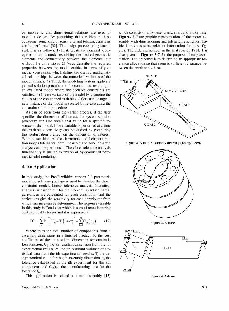
This application is related to motor assembly [13]

which consists of an x-base, crank, shaft and motor base. Figures 2-7 are graphic representation of the motor as-sembly with dimensioning and tolerancing schemes. Ta-ble 1 provides some relevant information for these fig-ures. The ordering number in the first row of Table 1 is also given in Figures 3-7 for the purpose of easy asso-ciation. The objective is to determine an appropriate tol-erance allocation so that there is sufficient clearance be-tween the crank and x-base.

Figure 2. A motor assembly drawing (Jeang, 1999).

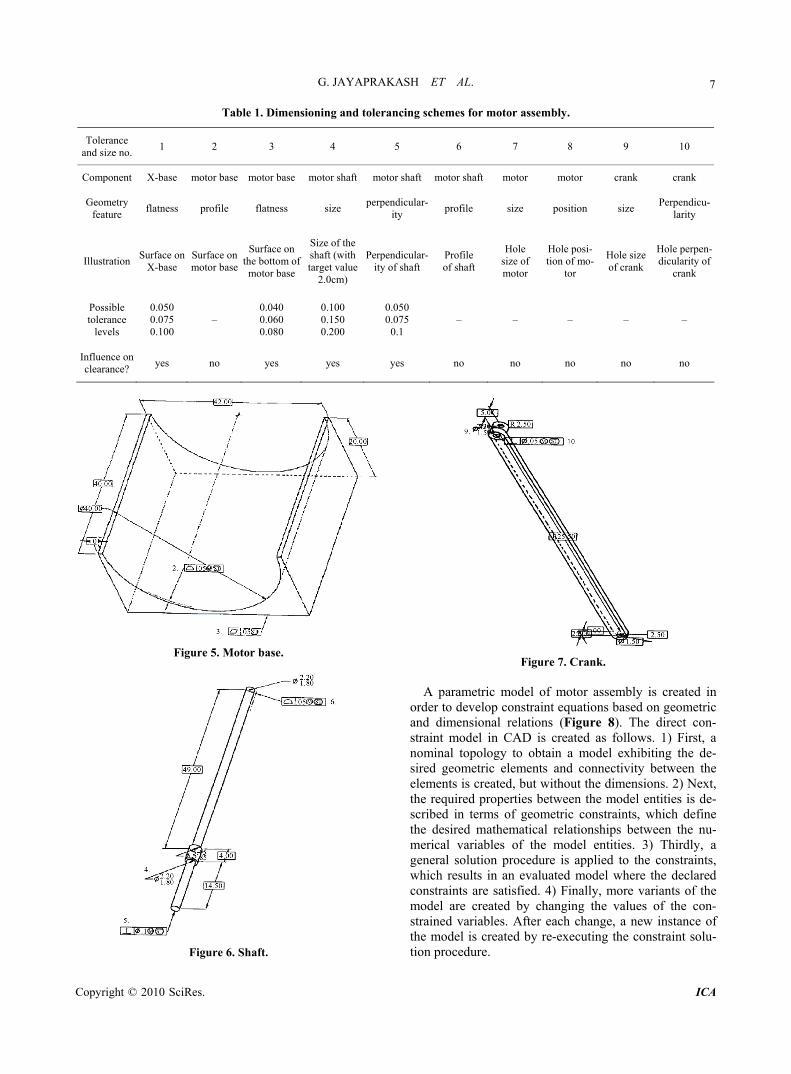
Figure 3. X-base.

Figure 4. X-base.



7

Table 1. Dimensioning and tolerancing schemes for motor assembly.

Tolerance and size no.

1 2 3 4 5 6 7 8 9 10

Component X-base motor base motor base motor shaft motor shaft motor shaft motor motor crank crank

Geometry feature

flatness profile flatness size perpendicular-

ity profile size position size

Perpendicu-larity

Illustration Surface on

X-base Surface on motor base

Surface on the bottom of motor base

Size of the shaft (with target value

2.0cm)

Perpendicular-ity of shaft

Profile of shaft

Hole size of motor

Hole posi-tion of mo-

tor

Hole size of crank

Hole perpen-dicularity of

crank

Possible tolerance

levels

0.050 0.075 0.100

– 0.040 0.060 0.080

0.100 0.150 0.200

0.050 0.075

0.1 – – – – –

Influence on clearance?

yes no yes yes yes no no no no no

Figure 5. Motor base.

Figure 6. Shaft.

Figure 7. Crank.

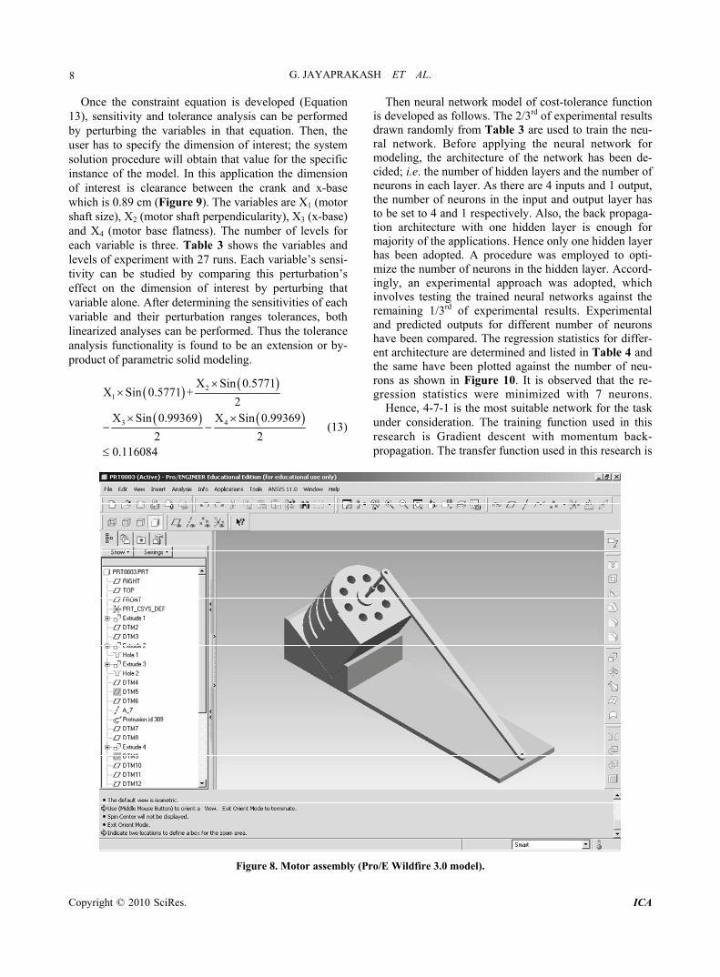
A parametric model of motor assembly is created in order to develop constraint equations based on geometric and dimensional relations (Figure 8). The direct con-straint model in CAD is created as follows. 1) First, a nominal topology to obtain a model exhibiting the de-sired geometric elements and connectivity between the elements is created, but without the dimensions. 2) Next, the required properties between the model entities is de-scribed in terms of geometric constraints, which define the desired mathematical relationships between the nu-merical variables of the model entities. 3) Thirdly, a general solution procedure is applied to the constraints, which results in an evaluated model where the declared constraints are satisfied. 4) Finally, more variants of the model are created by changing the values of the con-strained variables. After each change, a new instance of the model is created by re-executing the constraint solu-tion procedure.



8

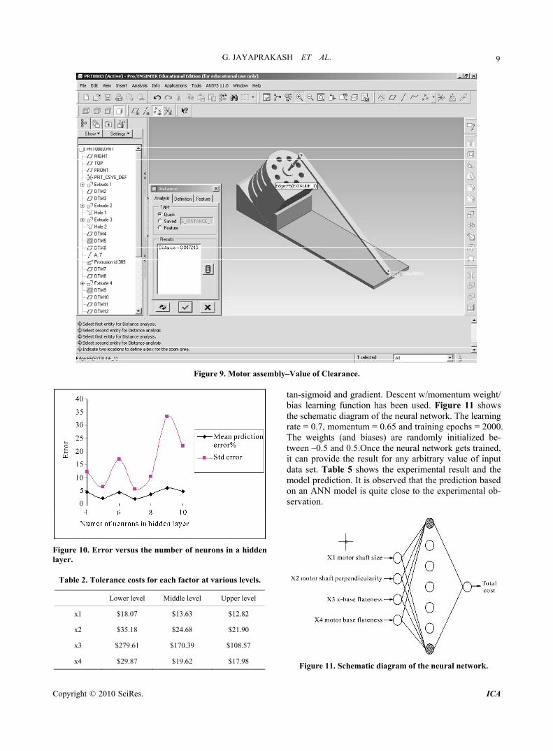
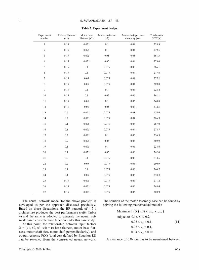
Once the constraint equation is developed (Equation 13), sensitivity and tolerance analysis can be performed by perturbing the variables in that equation. Then, the user has to specify the dimension of interest; the system solution procedure will obtain that value for the specific instance of the model. In this application the dimension of interest is clearance between the crank and x-base which is 0.89 cm (Figure 9). The variables are X1 (motor shaft size), X2 (motor shaft perpendicularity), X3 (x-base) and X4 (motor base flatness). The number of levels for each variable is three. Table 3 shows the variables and levels of experiment with 27 runs. Each variable’s sensi-tivity can be studied by comparing this perturbation’s effect on the dimension of interest by perturbing that variable alone. After determining the sensitivities of each variable and their perturbation ranges tolerances, both linearized analyses can be performed. Thus the tolerance analysis functionality is found to be an extension or by- product of parametric solid modeling.

21

3 4

X Sin 0.5771X Sin 0.5771 +

2X Sin 0.99369 X Sin 0.99369

2 20.116084

(13)

Then neural network model of cost-tolerance function is developed as follows. The 2/3rd of experimental results drawn randomly from Table 3 are used to train the neu-ral network. Before applying the neural network for modeling, the architecture of the network has been de-cided; i.e. the number of hidden layers and the number of neurons in each layer. As there are 4 inputs and 1 output, the number of neurons in the input and output layer has to be set to 4 and 1 respectively. Also, the back propaga-tion architecture with one hidden layer is enough for majority of the applications. Hence only one hidden layer has been adopted. A procedure was employed to opti-mize the number of neurons in the hidden layer. Accord-ingly, an experimental approach was adopted, which involves testing the trained neural networks against the remaining 1/3rd of experimental results. Experimental and predicted outputs for different number of neurons have been compared. The regression statistics for differ-ent architecture are determined and listed in Table 4 and the same have been plotted against the number of neu-rons as shown in Figure 10. It is observed that the re-gression statistics were minimized with 7 neurons.

Hence, 4-7-1 is the most suitable network for the task under consideration. The training function used in this research is Gradient descent with momentum back- propagation. The transfer function used in this research is

Figure 8. Motor assembly (Pro/E Wildfire 3.0 model).



9

Figure 9. Motor assembly–Value of Clearance.

Figure 10. Error versus the number of neurons in a hidden layer.

Table 2. Tolerance costs for each factor at various levels.

Lower level Middle level Upper level

x1 $18.07 $13.63 $12.82

x2 $35.18 $24.68 $21.90

x3 $279.61 $170.39 $108.57

x4 $29.87 $19.62 $17.98

tan-sigmoid and gradient. Descent w/momentum weight/ bias learning function has been used. Figure 11 shows the schematic diagram of the neural network. The learning rate = 0.7, momentum = 0.65 and training epochs = 2000. The weights (and biases) are randomly initialized be-tween –0.5 and 0.5.Once the neural network gets trained, it can provide the result for any arbitrary value of input data set. Table 5 shows the experimental result and the model prediction. It is observed that the prediction based on an ANN model is quite close to the experimental ob-servation.

Figure 11. Schematic diagram of the neural network.



10

Table 3. Experiment design.

Experiment number

X-Base Flatness (x1)

Motor base Flatness (x2)

Motor shaft size (x3)

Motor shaft perpen-dicularity (x4)

Total cost in $ TC(X)

1 0.15 0.075 0.1 0.08 228.9

2 0.15 0.075 0.1 0.04 239.5

3 0.15 0.075 0.05 0.08 361.3

4 0.15 0.075 0.05 0.04 373.0

5 0.15 0.1 0.075 0.08 266.1

6 0.15 0.1 0.075 0.04 277.6

7 0.15 0.05 0.075 0.08 277.2

8 0.15 0.05 0.075 0.04 289.0

9 0.15 0.1 0.1 0.06 228.4

10 0.15 0.1 0.05 0.06 361.1

11 0.15 0.05 0.1 0.06 240.8

12 0.15 0.05 0.05 0.06 372.5

13 0.2 0.075 0.075 0.08 274.6

14 0.2 0.075 0.075 0.04 286.3

15 0.1 0.075 0.075 0.08 267.0

16 0.1 0.075 0.075 0.04 278.7

17 0.2 0.075 0.1 0.06 236.3

18 0.2 0.075 0.05 0.06 369.9

19 0.1 0.075 0.1 0.06 228.6

20 0.1 0.075 0.05 0.06 362.0

21 0.2 0.1 0.075 0.06 274.6

22 0.2 0.05 0.075 0.06 290.9

23 0.1 0.1 0.075 0.06 266.7

24 0.1 0.05 0.075 0.06 278.3

25 0.15 0.075 0.075 0.06 271.2

26 0.15 0.075 0.075 0.06 268.4

27 0.15 0.075 0.075 0.06 269.9

The neural network model for the above problem is

developed as per the approach discussed previously. Based on those discussions, the BP network of 4-7-1 architecture produces the best performance (refer Table 4) and the same is adopted to generate the neural net-work based cost-tolerance function under this case study.

At this point, the relationship between input factors X = (x1, x2, x3, x4) = (x-base flatness, motor base flat-ness, motor shaft size, motor shaft perpendicularity), and output response F(X) (total cost defined by Equation 12) can be revealed from the constructed neural network.

The solution of the motor assembly case can be found by solving the following mathematical models:

1 2 3 4

1

2

3

4

MaximizeF X F x , x , x , x

subject to 0.1 x 0.2,

0.05 x 0.1,

0.05 x 0.1,

0.04 x 0.08

(14)

A clearance of 0.89 cm has to be maintained between



11

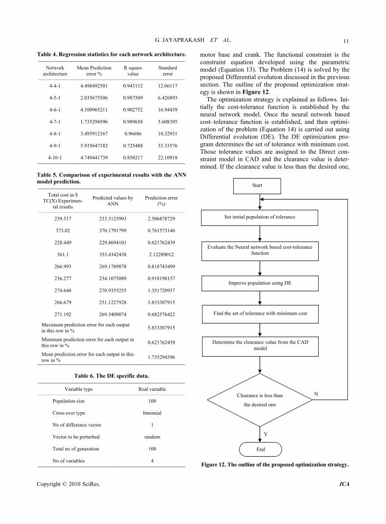
Table 4. Regression statistics for each network architecture.

Network architecture

Mean Prediction error %

R square value

Standard error

4-4-1 4.498492501 0.943112 12.06117

4-5-1 2.035675506 0.987509 6.426893

4-6-1 4.100965211 0.902752 16.94439

4-7-1 1.735294596 0.989658 5.608395

4-8-1 3.495912167 0.96686 10.32931

4-9-1 5.935647182 0.725488 33.33576

4-10-1 4.749441739 0.850217 22.10918

Table 5. Comparison of experimental results with the ANN model prediction.

Total cost in $ TC(X) Experimen-

tal results

Predicted values by ANN

Prediction error (%)

239.517 233.5125993 2.506878729

373.02 370.1791799 0.761573146

228.449 229.8694101 0.621762439

361.1 353.4342438 2.12289012

266.993 269.1789878 0.818743499

236.277 234.1075089 0.918198157

274.648 270.9355255 1.351720937

266.679 251.1227928 5.833307915

271.192 269.3409074 0.682576422

Maximum prediction error for each output in this row in %

5.833307915

Minimum prediction error for each output in this row in %

0.621762439

Mean prediction error for each output in this row in %

1.735294596

Table 6. The DE specific data.

Variable type Real variable

Population size 100

Cross over type binomial

No of difference vector 1

Vector to be perturbed random

Total no of generation 100

No of variables 4

motor base and crank. The functional constraint is the constraint equation developed using the parametric model (Equation 13). The Problem (14) is solved by the proposed Differential evolution discussed in the previous section. The outline of the proposed optimization strat-egy is shown in Figure 12.

The optimization strategy is explained as follows. Ini-tially the cost-tolerance function is established by the neural network model. Once the neural network based cost–tolerance function is established, and then optimi-zation of the problem (Equation 14) is carried out using Differential evolution (DE). The DE optimization pro-gram determines the set of tolerance with minimum cost. Those tolerance values are assigned to the Direct con-straint model in CAD and the clearance value is deter-mined. If the clearance value is less than the desired one,

Start

Set initial population of tolerance

Clearance is less than

the desired one

End

N

Y

Find the set of tolerance with minimum cost

Improve population using DE

Evaluate the Neural network based cost-tolerance function

Determine the clearance value from the CAD model

Figure 12. The outline of the proposed optimization strategy.



12

the process terminates, otherwise the process is repeated from the beginning.

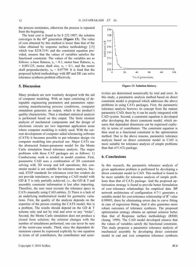
The least cost is found to be $ 232.1907; the solution converges in the 49th generation (Figure 13). The value of cost obtained by this method is lesser than that of the value obtained by response surface methodology [13] which was $238.5191 and the constraint equation pro-vided, ensures that the values of variables satisfies the functional constraint. The values of the variables are as follows. x-base flatness, x1 = 0.1, motor base flatness, x2

= 0.081125, motor shaft size, x3 = 0.1, and the motor shaft perpendicularity, x4 = 0.07799. It is fond that the proposed hybrid methodology with BP and DE can solve tolerance synthesis problem effectively. 5. Discussion Many products are now routinely designed with the aid of computer modeling. With an input consisting of de-signable engineering parameters and parameters repre-senting manufacturing process conditions, computer simulation generates an output, which is the product’s quality characteristic. Then a standard statistical analysis is performed based on this output. The finite element analysis of mechanical components and the design of electronic circuits are two important application areas where computer modeling is widely used. With the cur-rent development of computer aided tolerancing software (CATS) it becomes possible to put tolerance design via computer modeling into practical use. Major CATs use the abstracted feature-parameter model for the Monte Carlo simulation based tolerance analysis. The major problems with these CAT packages are as follows: 1) Cumbersome work is needed in model creation. First, parametric CAD uses a combination of 2D constraint solving with 3D sweep and loft operations; this con-straint model is not suitable for tolerance analysis. Sec-ond, STEP standards for tolerances exist but vendors do not provide translators, so importing a CAD model with GD & T is only partially achieved, i.e., the GD & T and assembly constraint information is lost after importing. Therefore, the user must recreate the tolerance specs in CATs manually using CAD entities. 2) There is a lack of an underlying mathematical model for geometric varia-tions. First, the quality of the analysis depends on the expertise of the person creating the CATS model; this is a problem. The results should depend on the GD & T scheme only and not by trial and error or any “tricks”. Second, the Monte Carlo simulation does not produce a closed form solution; the solution changes with the number of simulations performed; one can never be sure of the worst-case results. Third, since the dependent di-mensions cannot be expressed explicitly by one equation in terms of all contributors, the contributors and sensi-

Figure 13. Solution history. tivities are determined numerically by trial and error. In this study, a parametric analysis method based on direct constraint model is proposed which addresses the above problems in using CATs packages. First, the parametric tolerance analysis borrows its concept from the mature parametric CAD; there by it can be easily integrated with CAD system. Second, a constraint equation is developed after developing the direct constraint model, which en-sures that dependent dimension can be expressed explic-itly in terms of contributors. The constraint equation is then used as a functional constraint in the optimization method. Due to the above reasons, parametric tolerance analysis based on direct constraint model in CAD is more suitable for tolerance analysis of simple problems than that of CATs package.

6. Conclusions In this research, the parametric tolerance analysis of given application problem is performed by developing a direct constraint model in CAD. This method is found to be more suitable for tolerance analysis of simple prob-lems than that of CATs package. And the proposed op-timization strategy is found to provide better formulation of cost–tolerance relationships for empirical data. BP network architecture of configuration 4-7-1 generates a suitable model for cost-tolerance relationship of R2 value 0.99993, there by eliminating errors due to curve fitting in case of regression fitting. And it also generates more robust outcomes of tolerance synthesis. The proposed optimization strategy obtains an optimal solution better than that of Response surface methodology (RSM) (Jeang, 1999). The CAD model developed ensures that the values of variables satisfy the functional constraint. This study proposes a parametric tolerance analysis of mechanical assembly by developing direct constraint model in cad and cost competent tolerance synthesis



13

based on BP learning and DE based optimization algo-rithm. The constraint equation developed ensures that the proposed values of controllable factors (tolerances) sat-isfy the assembly constraint, even before the start of manufacturing process. There by reducing scrap and re-work cost.

7. References [1] J. Turner and A. B. Gangoiti, “Tolerance Analysis Ap-

proaches in Commercial Software,” Concurrent Engi-neering, Vol. 1, No. 2, 1991, pp.11-23.

[2] J. Guilford, M. Sethi and J. Turner, “Worst Case and Statistical Tolerance Analysis of the Daughter Card As-sembly,” Proceedings of the 1992 ASME International Computers in Engineering Conference, San Francisco, 2-6 August 1992, pp. 343-350.

[3] Y. Wu, J. Shah and J. Davidson, “Computer Modeling of Geometric Variations in Mechanical Parts and Assem-blies,” ASME Journal Computing and Information Sci-ence in Engineering, Vol. 3, No. 1, 2003, pp. 54-63.

[4] T. M. K. Pasupathy, E. P. Morse and R. G. Wilhelm, “A Survey of Mathematical Methods for the Construction of Geometric Tolerance Zones,” ASME Journal Computing and Information Science in Engineering, Special Issue on GD & T, Vol. 3, No. 1, 2003, pp. 64-75.

[5] P. Martino, “Simplification of Feature Based Models for Tolerance Analysis”, Proceedings of the 1992 ASME In-ternational Computers in Engineering Conference & Ex-position, San Francisco, 2-6 August 1992, pp. 329-341.

[6] Y.-J. Tseng and Y.-S. Terng, “Alternative Tolerance Al-locations for Machining Parts Represented with Multiple Sets of Features,” International Journal of Production Research, Vol. 37, No. 7, 1999, pp. 1561-1579.

[7] B. K. A. Ngoi and J. M. Ong, “A Complete Tolerance Charting System in Assembly,” International Journal of Production Research, Vol. 37, No. 11, 1999, pp. 2477- 2498.

[8] U. Prisco and G. Giorleo, “Overview of Current CAT Systems,” Integrated Computer-Aided Engineering, Vol. 9, No. 4, 2002, pp. 373-387.

[9] Z. Shen, “Software Review-Tolerance Analysis with EDS/VisVSA,” ASME Journal Computing and Informa-tion Science in Engineering, Special Issue on GD & T, Vol. 3, No. 1, 2003, pp. 95–99.

[10] F. Chiesi and L. Governi, “Software Review-Tolerance Analysis with eTol-Mate,” ASME Journal Computing and Information Science in Engineering, Special Issue on GD & T, Vol. 3, No. 1, 2003, pp. 100-105.

[11] C. X. Feng and A. Kusiak, “Design of Tolerances for Quality,” Design Theory and Methodology-DTM’ 94, Vol. 668, ASME, 1994, pp. 19-27.

[12] A. Jeang, “Tolerance Chart Optimisation for Quality and Cost,” International Journal of Production Research, Vo. 36. No. 11, 1998, pp. 2969-2983.

[13] A. Jeang, “Optimal Tolerance Design by Response Sur-

face Methodology,” International Journal of Production Research, Vol. 37, No. 14, 1999, pp. 3275-3288.

[14] C. C. Wu and G. R. Tang, “Tolerance Design for Prod-ucts with Asymmetric Quality Losses,” International Journal of Production Research, Vol. 36, No. 9, 1998, pp. 2529-2541.

[15] S. C. Diplaris and M. M. Sfantsikopoulos, “Tolerancing for Enhanced Quality and Optimum Cost,” Proceedings of the 33rd International MATADOR Conference, Man-chester, 1999, pp. 539-544.

[16] A. Jeang, “An Approach of Tolerance Design for Quality Improvement and Cost Reduction”, International Journal of Production Research, Vol. 35, No. 5, 1997, pp. 1193- 1211.

[17] F. H. Speckhart, “Calculation of Tolerance Based on Minimum Cost Approach,” Journal of Engineering for Industry-Transactions of the ASME, Vol. 94, No. 2, 1972, pp. 447-453.

[18] M. F. Spotts, “Allocation of Tolerances to Minimize Cost of Assembly,” Journal of Engineering for Indus-try-Transactions of the ASME, Vol. 95, No. 3, 1973, pp. 762-764.

[19] K. W. Chase, W. H. Greenwood, B. G. Loosli and L. F. Hauglund, “Least Cost Tolerance Allocation for Me-chanical Assemblies with Automated Process Selection,” Manufacturing Review, Vol. 3, No. 1, 1990, pp. 49-59.

[20] Z. Dong, W. Hu and D. Xue, “New Production Cost Tol-erance Models for Tolerance Synthesis,” Journal of the Engineering Industry, Vol. 116, 1994, pp. 199-205.

[21] R. Soderberg, “Robust Design by Tolerance Allocation Considering Quality and Manufacturing Cost,” Advances in Design Automation, Vol. 69-1, ASME, 1994, pp. 219- 226.

[22] M. Krishnasawamy and R. W. Mayne, “Optimizing Tol-erance Allocation Based on Manufacturing Cost,” Ad-vances in Design Automation, Vol. 69-1, ASME, 1994, pp. 211-217.

[23] E. M. Mansoor, “The Application of Probability to Tol-erances Used in Engineering Design,” Proceedings of the Institution of Mechanical Engineers, Vol. 178, No. 1, 1963, pp. 29-44.

[24] E. Santoro, “Probabilistic Model for Tolerance Synthesis: An Analytical Solution, Structural Safety and Reliabil-ity,” Balkema, Rotterdam, 1994.

[25] V. J. Skowronski and J. U. Turner, “Estimating Gradients for Statistical Tolerance Synthesis,” Computer-Aided De-sign, Vol. 28, No. 12, 1996, pp. 933-941.

[26] C. Zhang, J. Luo and B. Wang, “Statistical Tolerance Synthesis Using Distribution Function Zones,” Interna-tional Journal of Production Research, Vol. 37, No. 17, 1999, pp. 3995-4006.

[27] M. H. Gaddalah and H.A. ElMaraghy, “The Tolerance Optimization Problem Using a System of Experimental Design,” Advances in Design Automation, Vol. 69-1, ASME, 1994, pp. 251-264.

[28] V. J. Skowronski and J. U. Turner, “Using Monte–Carlo Variance Reduction in Statistical Tolerance Synthesis,”



14

Computer-Aided Design, Vol. 29, No. 1, 1997, pp. 63-69.

[29] H. S. Stern, “Neural Networks in Applied Statistics (with Discussion),” Technometrics, Vol. 38, No. 3, 1996, pp. 205-220.

[30] H.-C. Zhang, H. Huang, “Applications of Neural Net-works in Manufacturing: A-State-of-the-Art Survey,” In-ternational Journal of Production Research, Vol. 33, No. 3, 1995, pp. 705-728.

[31] D. E. Rumelhart and J. L. McClelland, “Parallel Distrib-

uted Processing Explorations in the Microstructure of Cognition,” MIT Press, Cambridge, 1989.

[32] R. P. Lippmann, “An Introduction to Computing with Neural Nets,” IEEE ASSP Magazine, Vol. 4, No. 2, 1987, pp. 4-22.

[33] K. Price and R. Storn, “Differential Evolution–A Simple Evolution Strategy for Fast Optimization,” Dr. Dobb’s Journal, Vol. 22, No. 4, pp.18-24 and 78.

Documents

Parametric Tolerance Analysis of Mechanical Assembly …file.scirp.org/pdf/ICA20100100001_51724716.pdf · Parametric Tolerance Analysis of Mechanical Assembly by ... balance manufacturing