Embed Size (px)
Citation preview
Parametric modelling of the cumulative
incidence function in competing risks models
Paul C Lambert1,2
1Department of Health Sciences,University of Leicester, UK
2 Department of Medical Epidemiology and Biostatistics,Karolinska Institutet, Stockholm, Sweden
Fundamental Problems in Survival AnalysisLondon 4/06/2014
Modelling with competing risks data
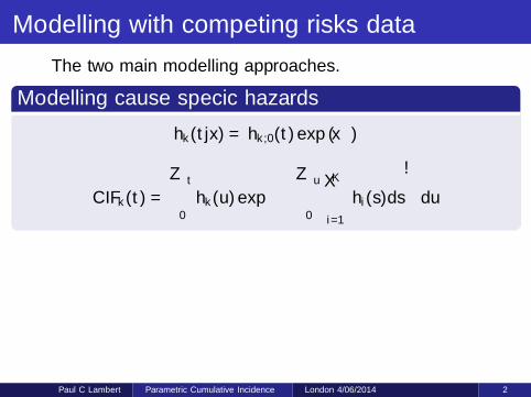
The two main modelling approaches.
Modelling cause specific hazards
hk(t|x) = hk,0(t) exp (xβ)
CIFk(t) =
∫ t
0
hk(u) exp
(−∫ u
0
K∑i=1
hi(s)ds
)du
Modelling subhazard
h∗k(t) =d log (1− CIFk(t))
dt
h∗k(t|x) = h∗k,0(t) exp (xβ)
My preference is to use (flexible) parametric models.
Paul C Lambert Parametric Cumulative Incidence London 4/06/2014 2
Modelling with competing risks data
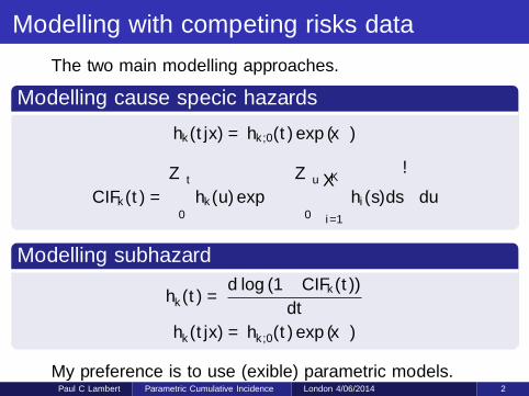
The two main modelling approaches.
Modelling cause specific hazards
hk(t|x) = hk,0(t) exp (xβ)
CIFk(t) =
∫ t
0
hk(u) exp
(−∫ u
0
K∑i=1
hi(s)ds
)du
Modelling subhazard
h∗k(t) =d log (1− CIFk(t))
dt
h∗k(t|x) = h∗k,0(t) exp (xβ)
My preference is to use (flexible) parametric models.Paul C Lambert Parametric Cumulative Incidence London 4/06/2014 2
Outline of the rest of the talk
1 Flexible parametric models
2 Modelling cause-specific hazards (brief)
3 Modelling cumulative incidence functions.
Paul C Lambert Parametric Cumulative Incidence London 4/06/2014 3
European Blood and Marrow Transplantation Data
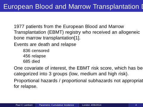
1977 patients from the European Blood and MarrowTransplantation (EBMT) registry who received an allogeneicbone marrow transplantation[1].
Events are death and relapse
836 censored456 relapse685 died
One covariate of interest, the EBMT risk score, which has beencategorized into 3 groups (low, medium and high risk).
Proportional hazards / proportional subhazards not appropriatefor relapse.
Paul C Lambert Parametric Cumulative Incidence London 4/06/2014 4
Cumulative Incidence Functions
0.0
0.1
0.2
0.3
0.4
0.5
CIF
0 2 4 6Years since transplantation
Low Risk
Medium Risk
High Risk
Relapse
0.0
0.1
0.2
0.3
0.4
0.5
CIF
0 2 4 6Years since transplantation
Low Risk
Medium Risk
High Risk
Died
Paul C Lambert Parametric Cumulative Incidence London 4/06/2014 5
Parametric Models
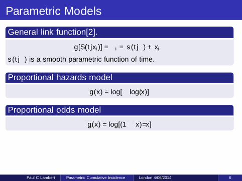
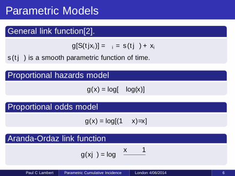
General link function[2].
g [S(t|xi)] = ηi = s (t|γ) + xiβ
s (t|γ) is a smooth parametric function of time.
Proportional hazards model
g(x) = log[− log(x)]
Proportional odds model
g(x) = log[(1− x)/x ]
Aranda-Ordaz link function
g(x |θ) = log
(x−θ − 1
θ
)
Paul C Lambert Parametric Cumulative Incidence London 4/06/2014 6
Parametric Models
General link function[2].
g [S(t|xi)] = ηi = s (t|γ) + xiβ
s (t|γ) is a smooth parametric function of time.
Proportional hazards model
g(x) = log[− log(x)]
Proportional odds model
g(x) = log[(1− x)/x ]
Aranda-Ordaz link function
g(x |θ) = log
(x−θ − 1
θ
)Paul C Lambert Parametric Cumulative Incidence London 4/06/2014 6
Parametric models
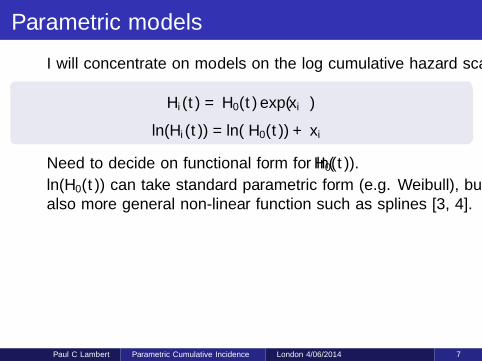
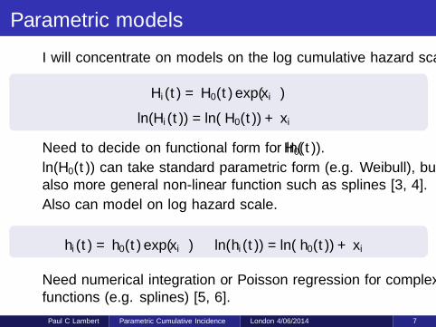
I will concentrate on models on the log cumulative hazard scale.
Hi(t) = H0(t) exp(xiβ)
ln(Hi(t)) = ln(H0(t)) + xiβ
Need to decide on functional form for ln(H0(t)).
ln(H0(t)) can take standard parametric form (e.g. Weibull), butalso more general non-linear function such as splines [3, 4].
Also can model on log hazard scale.
hi(t) = h0(t) exp(xiβ) ln(hi(t)) = ln(h0(t)) + xiβ
Need numerical integration or Poisson regression for complexfunctions (e.g. splines) [5, 6].
Paul C Lambert Parametric Cumulative Incidence London 4/06/2014 7
Parametric models
I will concentrate on models on the log cumulative hazard scale.
Hi(t) = H0(t) exp(xiβ)
ln(Hi(t)) = ln(H0(t)) + xiβ
Need to decide on functional form for ln(H0(t)).
ln(H0(t)) can take standard parametric form (e.g. Weibull), butalso more general non-linear function such as splines [3, 4].
Also can model on log hazard scale.
hi(t) = h0(t) exp(xiβ) ln(hi(t)) = ln(h0(t)) + xiβ
Need numerical integration or Poisson regression for complexfunctions (e.g. splines) [5, 6].
Paul C Lambert Parametric Cumulative Incidence London 4/06/2014 7

Flexible parametric models: basic idea
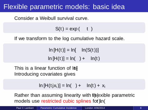
Consider a Weibull survival curve.
S(t) = exp (−λtγ)
If we transform to the log cumulative hazard scale.
ln [H(t)] = ln[− ln(S(t))]
ln [H(t)] = ln(λ) + γ ln(t)
This is a linear function of ln(t)
Introducing covariates gives
ln [H(t|xi)] = ln(λ) + γ ln(t) + xiβ
Rather than assuming linearity with ln(t) flexible parametricmodels use restricted cubic splines for ln(t).
Paul C Lambert Parametric Cumulative Incidence London 4/06/2014 8
Flexible parametric models: basic idea
Consider a Weibull survival curve.
S(t) = exp (−λtγ)
If we transform to the log cumulative hazard scale.
ln [H(t)] = ln[− ln(S(t))]
ln [H(t)] = ln(λ) + γ ln(t)
This is a linear function of ln(t)Introducing covariates gives
ln [H(t|xi)] = ln(λ) + γ ln(t) + xiβ
Rather than assuming linearity with ln(t) flexible parametricmodels use restricted cubic splines for ln(t).
Paul C Lambert Parametric Cumulative Incidence London 4/06/2014 8
Flexible parametric models: incorporating splines
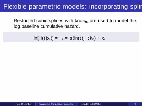
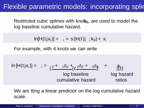
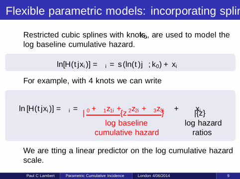
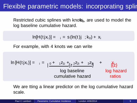
Restricted cubic splines with knots, k0, are used to model thelog baseline cumulative hazard.
ln[H(t|xi)] = ηi = s (ln(t)|γ, k0) + xiβ
For example, with 4 knots we can write
ln [H(t|xi)] = ηi = γ0 + γ1z1i + γ2z2i + γ3z3i︸ ︷︷ ︸log baseline
cumulative hazard
+ xiβ︸︷︷︸log hazard
ratios
We are fitting a linear predictor on the log cumulative hazardscale.
Paul C Lambert Parametric Cumulative Incidence London 4/06/2014 9
Flexible parametric models: incorporating splines
Restricted cubic splines with knots, k0, are used to model thelog baseline cumulative hazard.
ln[H(t|xi)] = ηi = s (ln(t)|γ, k0) + xiβ
For example, with 4 knots we can write
ln [H(t|xi)] = ηi = γ0 + γ1z1i + γ2z2i + γ3z3i︸ ︷︷ ︸log baseline
cumulative hazard
+ xiβ︸︷︷︸log hazard
ratios
We are fitting a linear predictor on the log cumulative hazardscale.
Paul C Lambert Parametric Cumulative Incidence London 4/06/2014 9
Survival and Hazard Functions
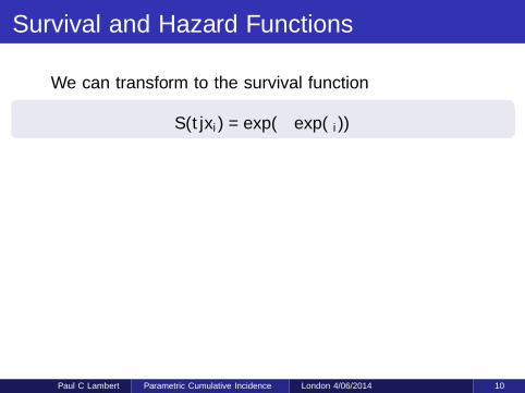
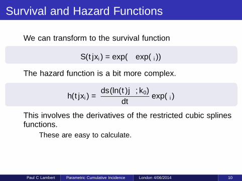
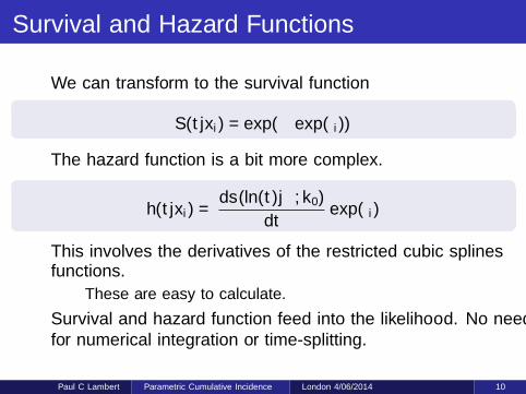
We can transform to the survival function
S(t|xi) = exp(− exp(ηi))
The hazard function is a bit more complex.
h(t|xi) =ds (ln(t)|γ, k0)
dtexp(ηi)
This involves the derivatives of the restricted cubic splinesfunctions.
These are easy to calculate.
Survival and hazard function feed into the likelihood. No needfor numerical integration or time-splitting.
Paul C Lambert Parametric Cumulative Incidence London 4/06/2014 10
Survival and Hazard Functions
We can transform to the survival function
S(t|xi) = exp(− exp(ηi))
The hazard function is a bit more complex.
h(t|xi) =ds (ln(t)|γ, k0)
dtexp(ηi)
This involves the derivatives of the restricted cubic splinesfunctions.
These are easy to calculate.
Survival and hazard function feed into the likelihood. No needfor numerical integration or time-splitting.
Paul C Lambert Parametric Cumulative Incidence London 4/06/2014 10
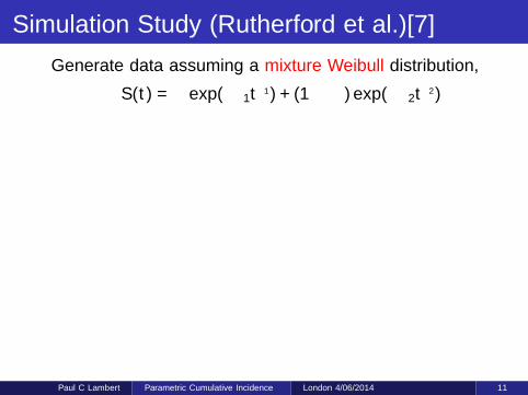
Simulation Study (Rutherford et al.)[7]
Generate data assuming a mixture Weibull distribution,
S(t) = π exp(−λ1tγ1) + (1− π) exp(−λ2t
γ2)
0.0
0.5
1.0
1.5
2.0
2.5
Haz
ard
rate
0 2 4 6 8 10Time Since Diagnosis (Years)
Scenario 1
0.0
0.5
1.0
1.5
2.0
2.5
Haz
ard
rate
0 2 4 6 8 10Time Since Diagnosis (Years)
Scenario 2
0.0
0.5
1.0
1.5
2.0
2.5
Haz
ard
rate
0 2 4 6 8 10Time Since Diagnosis (Years)
Scenario 3
0.0
0.5
1.0
1.5
2.0
2.5
Haz
ard
rate
0 2 4 6 8 10Time Since Diagnosis (Years)
Scenario 4
Fit models using restricted cubic splines.
Paul C Lambert Parametric Cumulative Incidence London 4/06/2014 11
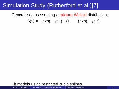
Simulation Study (Rutherford et al.)[7]
Generate data assuming a mixture Weibull distribution,
S(t) = π exp(−λ1tγ1) + (1− π) exp(−λ2t
γ2)
0.0
0.5
1.0
1.5
2.0
2.5H
azar
d ra
te
0 2 4 6 8 10Time Since Diagnosis (Years)
Scenario 1
0.0
0.5
1.0
1.5
2.0
2.5
Haz
ard
rate
0 2 4 6 8 10Time Since Diagnosis (Years)
Scenario 2
0.0
0.5
1.0
1.5
2.0
2.5
Haz
ard
rate
0 2 4 6 8 10Time Since Diagnosis (Years)
Scenario 3
0.0
0.5
1.0
1.5
2.0
2.5
Haz
ard
rate
0 2 4 6 8 10Time Since Diagnosis (Years)
Scenario 4
Fit models using restricted cubic splines.Paul C Lambert Parametric Cumulative Incidence London 4/06/2014 11
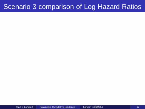
Scenario 3 comparison of Log Hazard Ratios
-.6
-.55
-.5
-.45
-.4C
ox M
odel
-.6 -.55 -.5 -.45 -.4Flexible Parametric Model
Paul C Lambert Parametric Cumulative Incidence London 4/06/2014 12

Scenario 3 comparison of Log Hazard Ratios
-.6
-.55
-.5
-.45
-.4C
ox M
odel
-.6 -.55 -.5 -.45 -.4Flexible Parametric Model
Paul C Lambert Parametric Cumulative Incidence London 4/06/2014 12
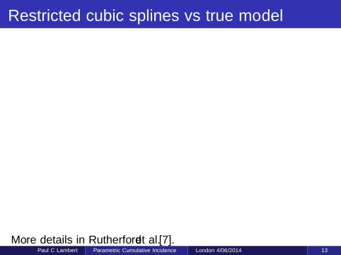
Restricted cubic splines vs true model
0
5
10
15
20
25
Perc
enta
ge o
f T
ota
l A
rea D
iffe
rence
on t
he S
urv
ival S
cale
1 2 3 4 5 6 7 8 9 10Degrees of Freedom
Sample Size 300
Sample Size 3000
Sample Size 30,000
Scenario 3
More details in Rutherford et al.[7].Paul C Lambert Parametric Cumulative Incidence London 4/06/2014 13
Modelling Cause-specific hazards
ln[Hk(t|xi)] = ln [Hk,0(t)] + xiβ
Fit all K causes simultaneously.
Can share parameters across causes.
Can incorporate time dependent effects for some covariates.
Parametric functions for hazard/survival functions.
CIF (and standard error) obtained using numerical integration.
CIFk(t) =
∫ t
0
hk(u) exp
(−
K∑i=1
Hi(u)
)du
See Hinchliffe et al. [8]
Paul C Lambert Parametric Cumulative Incidence London 4/06/2014 14
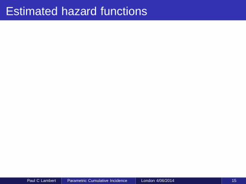
Estimated hazard functions
0
200
400
600
800
Rel
apse
Rat
e (p
er 1
000
py)
0 2 4 6Years since transplantation
Low Risk
Medium Risk
High Risk
Relapse
0
200
400
600
800
1000
1200
Mor
talit
y R
ate
(per
100
0 py
)
0 2 4 6Years since transplantation
Low Risk
Medium Risk
High Risk
Death
Paul C Lambert Parametric Cumulative Incidence London 4/06/2014 15
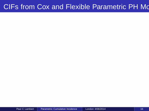
CIFs from Cox and Flexible Parametric PH Models
0.0
0.1
0.2
0.3
0.4
0.5
CIF
0 2 4 6Years since transplantation
Low Risk
Medium Risk
High Risk
Relapse
0.0
0.1
0.2
0.3
0.4
0.5
CIF
0 2 4 6Years since transplantation
Low Risk
Medium Risk
High Risk
Died
Paul C Lambert Parametric Cumulative Incidence London 4/06/2014 16

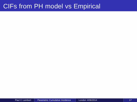
CIFs from PH model vs Empirical
0.0
0.1
0.2
0.3
0.4C
IF
0 2 4 6Years since transplantation
Low RiskMedium RiskHigh Risk
Relapse
Paul C Lambert Parametric Cumulative Incidence London 4/06/2014 17
CIFs from PH model vs Empirical
0.0
0.1
0.2
0.3
0.4C
IF
0 2 4 6Years since transplantation
Low RiskMedium RiskHigh Risk
Relapse
Paul C Lambert Parametric Cumulative Incidence London 4/06/2014 17
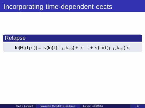
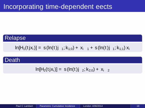
Incorporating time-dependent effects
Relapse
ln[H1(t|xi)] = s (ln(t)|γ1, k1,0) + xiβ1 + s (ln(t)|δ1, k1,1) xi
Death
ln[H2(t|xi)] = s (ln(t)|γ2, k2,0) + xiβ2
Paul C Lambert Parametric Cumulative Incidence London 4/06/2014 18
Incorporating time-dependent effects
Relapse
ln[H1(t|xi)] = s (ln(t)|γ1, k1,0) + xiβ1 + s (ln(t)|δ1, k1,1) xi
Death
ln[H2(t|xi)] = s (ln(t)|γ2, k2,0) + xiβ2
Paul C Lambert Parametric Cumulative Incidence London 4/06/2014 18

Hazard functions for relapse
0
200
400
600
800R
elap
se R
ate
(100
0 py
)
0 2 4 6Years since transplantation
Low RiskMedium RiskHigh Risk
Relapse
Paul C Lambert Parametric Cumulative Incidence London 4/06/2014 19
Hazard functions for relapse
0
200
400
600
800R
elap
se R
ate
(100
0 py
)
0 2 4 6Years since transplantation
Low RiskMedium RiskHigh Risk
Relapse
Paul C Lambert Parametric Cumulative Incidence London 4/06/2014 19

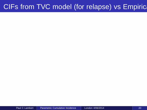
CIFs from TVC model (for relapse) vs Empirical
0.0
0.1
0.2
0.3
0.4C
IF
0 2 4 6Years since transplantation
Low RiskMedium RiskHigh Risk
Relapse
Paul C Lambert Parametric Cumulative Incidence London 4/06/2014 20
CIFs from TVC model (for relapse) vs Empirical
0.0
0.1
0.2
0.3
0.4C
IF
0 2 4 6Years since transplantation
Low RiskMedium RiskHigh Risk
Relapse
Paul C Lambert Parametric Cumulative Incidence London 4/06/2014 20
Model Cumulative Incidence Functions
Now switch to modelling the CIF directly
Aim:
Predict CIF for individual subjects.Direct covariate effects on CIF.Use different link functions.Model non-proportional effects.Be able to fit to large data sets.
Paul C Lambert Parametric Cumulative Incidence London 4/06/2014 21
Geskus (Biometrics 2011) Approach
Geskus (2011) showed that weighted versions of standardsurvival analysis procedures can be used to estimate the CIF[9].
Uses inverse probability of censoring weights.
Weights are time-dependent so data is expanded for subjectswith competing events.
After data expansion
Weighted Kaplan-Meier gives product-limit estimate of CIF.Weighted Cox model gives Fine and Gray model.
crprep in R and stcrprep in Stata.
Using similar weights in a likelihood based setting enablesstandard parametric models to be used to directly model the CIF.
Paul C Lambert Parametric Cumulative Incidence London 4/06/2014 22
Data expansion and weighting
Define event of interest.
Subjects that have a competing event are kept in the risk set tothe end of follow-up.
However, there is a a chance that they would be censored aftertheir competing event.
Estimate censoring distribution.
Weights depend on conditional probability of not being censoredafter competing event.
Paul C Lambert Parametric Cumulative Incidence London 4/06/2014 23

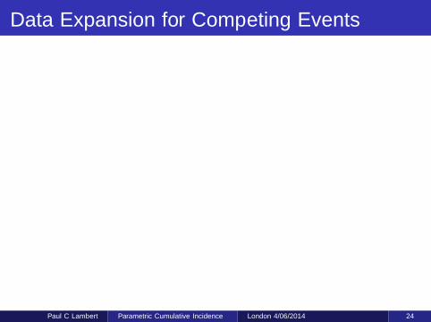
Data Expansion for Competing Events
9
8
7
6
5
4
3
2
1
Time
Censored Cancer Other
Paul C Lambert Parametric Cumulative Incidence London 4/06/2014 24

Data Expansion for Competing Events
9
8
7
6
5
4
3
2
1
Time
Censored Cancer Other
Paul C Lambert Parametric Cumulative Incidence London 4/06/2014 24
Data Expansion for Competing Events
w81 w82 w83 w84
w41 w42
9
8
7
6
5
4
3
2
1
Time
Censored Cancer Other
Paul C Lambert Parametric Cumulative Incidence London 4/06/2014 24

Data Expansion for Competing Events
w81 w82 w83 w84
w41 w42
9
8
7
6
5
4
3
2
1
Time
Censored Cancer Other
Paul C Lambert Parametric Cumulative Incidence London 4/06/2014 24
Large datasets
I analyse registry data, which is often large.
Datasets of 500,000 is not unusual.
Method needs to be usable in these large datasets.
Paul C Lambert Parametric Cumulative Incidence London 4/06/2014 25
Parametric approach
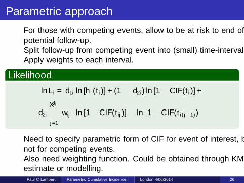
For those with competing events, allow to be at risk to end ofpotential follow-up.Split follow-up from competing event into (small) time-intervals.Apply weights to each interval.
Likelihood
ln Li = d1i ln [h∗(ti)] + (1− d2i) ln [1− CIF (ti)] +
d2i
Ji∑j=1
wij
(ln [1− CIF (tij)]− ln
[1− CIF (ti(j−1))
])Need to specify parametric form of CIF for event of interest, butnot for competing events.Also need weighting function. Could be obtained through KMestimate or modelling.
Paul C Lambert Parametric Cumulative Incidence London 4/06/2014 26

Splitting
Censored
Event 2
Event 1
Time
Paul C Lambert Parametric Cumulative Incidence London 4/06/2014 27

Splitting
Censored
Event 2
Event 1
Time
Paul C Lambert Parametric Cumulative Incidence London 4/06/2014 27
Splitting
Censored
Event 2
Event 1
Time
Paul C Lambert Parametric Cumulative Incidence London 4/06/2014 27

Splitting
w1 w2 w3 w4 w5
Censored
Event 2
Event 1
Time
Paul C Lambert Parametric Cumulative Incidence London 4/06/2014 27
The censoring distribution
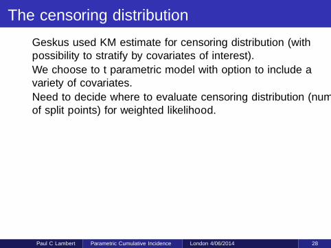
Geskus used KM estimate for censoring distribution (withpossibility to stratify by covariates of interest).
We choose to fit parametric model with option to include avariety of covariates.
Need to decide where to evaluate censoring distribution (numberof split points) for weighted likelihood.
0.0
0.2
0.4
0.6
0.8
1.0
S(t
)
0 2 4 6 8Years since transplantation
Kaplan-MeierParametric Model
Paul C Lambert Parametric Cumulative Incidence London 4/06/2014 28

The censoring distribution
Geskus used KM estimate for censoring distribution (withpossibility to stratify by covariates of interest).
We choose to fit parametric model with option to include avariety of covariates.
Need to decide where to evaluate censoring distribution (numberof split points) for weighted likelihood.
0.0
0.2
0.4
0.6
0.8
1.0
S(t
)
0 2 4 6 8Years since transplantation
Kaplan-MeierParametric Model
Paul C Lambert Parametric Cumulative Incidence London 4/06/2014 28
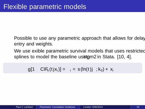
Flexible parametric models
Possible to use any parametric approach that allows for delayedentry and weights.
We use flexible parametric survival models that uses restrictedsplines to model the baseline using stpm2 in Stata. [10, 4].
g [1− CIFk(t|xi)] = ηi = s (ln(t)|γ, k0) + xiβ
Paul C Lambert Parametric Cumulative Incidence London 4/06/2014 29
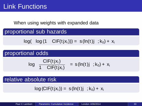
Link Functions
When using weights with expanded data
proportional sub hazards
log(− log (1− CIF (t|xi))) = s (ln(t)|γ, k0) + xiβ
proportional odds
log
(CIF (t|xi)
1− CIF (t|xi)
)= s (ln(t)|γ, k0) + xiβ
relative absolute risk
log (CIF (t|xi)) = s (ln(t)|γ, k0) + xiβ
Paul C Lambert Parametric Cumulative Incidence London 4/06/2014 30
Simulation
When using splines we are never fitting the ‘true’ model.
When assessing performance using simulation we simulate froma complex hazard function and then compare the truth to ourapproximation using splines.
For this study we simulated data as follows,
2 types of events. Event 1 of primary interest.Subhazard for event 1 from mixture Weibull distribution.Cause-specific hazard for event 2 from mixture Weibulldistribution.Using a combination of numerical integration and root finding itis possible to obtain the cause-specific hazard for event 1.
Paul C Lambert Parametric Cumulative Incidence London 4/06/2014 31
Simulation
Given cause-specific hazards for both causes use methods ofBeyersmann[11] to simulate data.
Based on general survival simulation algorithm, Crowther et al.2013 [12]
Follow-up restricted to 5 years.
Censoring distribution generated from Weibull distribution.
Probability of censoring by 5 years 0.3-0.4.
1000 simulated datasets for each scenario.
Flexible Parametric models with 3, 5 and 7 df for baseline fitted.
Splits every 0.01, 0.1, 0.2, 0.5 and 1 years used for weighting.
Paul C Lambert Parametric Cumulative Incidence London 4/06/2014 32

Scenario 4
0.00
0.10
0.20
0.30
0.40
CIF
0 1 2 3 4 5Time
x=0
x=1
Cause 1: CIF
0.00
0.05
0.10
0.15
caus
e-sp
ecifi
c su
bhaz
ard
rate
0 1 2 3 4 5Time
x=0
x=1
Cause 1: subhazard rate
Paul C Lambert Parametric Cumulative Incidence London 4/06/2014 33
Scenario 4
0.00
0.10
0.20
0.30
0.40
CIF
0 1 2 3 4 5Time
x=0
x=1
Cause 1: CIF
0.00
0.05
0.10
0.15
caus
e-sp
ecifi
c su
bhaz
ard
rate
0 1 2 3 4 5Time
x=0
x=1
Cause 1: subhazard rate
0.040
0.060
0.080
0.100
0.120
caus
e-sp
ecifi
c ha
zard
rat
e
0 1 2 3 4 5Time
x=0
x=1
Cause 2: cause-specific hazard
Paul C Lambert Parametric Cumulative Incidence London 4/06/2014 33

Scenario 4
0.00
0.10
0.20
0.30
0.40
CIF
0 1 2 3 4 5Time
x=0
x=1
Cause 1: CIF
0.00
0.05
0.10
0.15
caus
e-sp
ecifi
c su
bhaz
ard
rate
0 1 2 3 4 5Time
x=0
x=1
Cause 1: subhazard rate
0.040
0.060
0.080
0.100
0.120
caus
e-sp
ecifi
c ha
zard
rat
e
0 1 2 3 4 5Time
x=0
x=1
Cause 2: cause-specific hazard
0.000
0.050
0.100
0.150
caus
e-sp
ecifi
c ha
zard
rat
e
0 1 2 3 4 5Time
x=0
x=1
Cause 1: cause-specific hazard
Paul C Lambert Parametric Cumulative Incidence London 4/06/2014 33
Scenario 4 Bias: Simulation Results
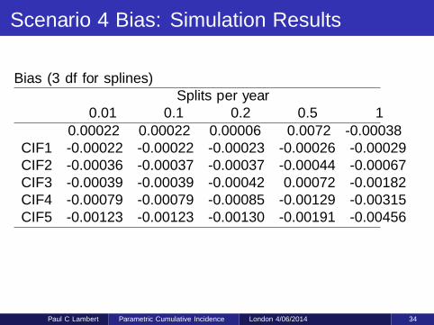
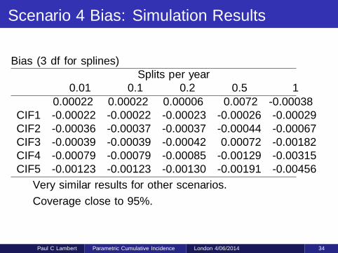
Bias (3 df for splines)Splits per year
0.01 0.1 0.2 0.5 1β 0.00022 0.00022 0.00006 0.0072 -0.00038CIF1 -0.00022 -0.00022 -0.00023 -0.00026 -0.00029CIF2 -0.00036 -0.00037 -0.00037 -0.00044 -0.00067CIF3 -0.00039 -0.00039 -0.00042 0.00072 -0.00182CIF4 -0.00079 -0.00079 -0.00085 -0.00129 -0.00315CIF5 -0.00123 -0.00123 -0.00130 -0.00191 -0.00456
Very similar results for other scenarios.
Coverage close to 95%.
Paul C Lambert Parametric Cumulative Incidence London 4/06/2014 34
Scenario 4 Bias: Simulation Results
Bias (3 df for splines)Splits per year
0.01 0.1 0.2 0.5 1β 0.00022 0.00022 0.00006 0.0072 -0.00038CIF1 -0.00022 -0.00022 -0.00023 -0.00026 -0.00029CIF2 -0.00036 -0.00037 -0.00037 -0.00044 -0.00067CIF3 -0.00039 -0.00039 -0.00042 0.00072 -0.00182CIF4 -0.00079 -0.00079 -0.00085 -0.00129 -0.00315CIF5 -0.00123 -0.00123 -0.00130 -0.00191 -0.00456
Very similar results for other scenarios.
Coverage close to 95%.
Paul C Lambert Parametric Cumulative Incidence London 4/06/2014 34
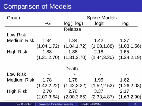
Comparison of Models
Group Spline ModelsFG log(− log) logit log
RelapseLow Risk - - - -Medium Risk 1.34 1.34 1.42 1.27
(1.04,1.72) (1.04,1.72) (1.08,1.88) (1.03,1.56)High Risk 1.88 1.88 2.18 1.65
(1.31,2.70) (1.31,2.70) (1.44,3.30) (1.24,2.19)
DeathLow Risk - - - -Medium Risk 1.78 1.78 1.95 1.62
(1.42,2.22) (1.42,2.22) (1.52,2.52) (1.26,2.08)High Risk 2.70 2.70 3.37 2.17
(2.00,3.64) (2.00,3.65) (2.33,4.87) (1.63,2.90)
Paul C Lambert Parametric Cumulative Incidence London 4/06/2014 35
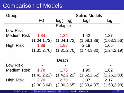
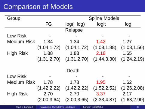
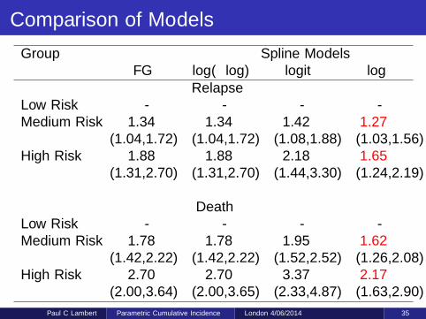
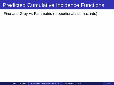
Predicted Cumulative Incidence Functions
Fine and Gray vs Parametric (proportional sub hazards)
0.0
0.1
0.2
0.3
0.4
0.5
Cum
ulat
ive
Inci
denc
e
0 1 2 3 4 5Years since transplantation
Relapse
0.0
0.1
0.2
0.3
0.4
0.5
Cum
ulat
ive
Inci
denc
e
0 1 2 3 4 5Years since transplantation
Death
Low Risk Medium Risk High Risk
Paul C Lambert Parametric Cumulative Incidence London 4/06/2014 36

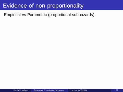
Evidence of non-proportionality
Empirical vs Parametric (proportional subhazards)
0.0
0.1
0.2
0.3
0.4
0.5
Cum
ulat
ive
Inci
denc
e
0 1 2 3 4 5Years since transplantation
Relapse
0.0
0.1
0.2
0.3
0.4
0.5
Cum
ulat
ive
Inci
denc
e
0 1 2 3 4 5Years since transplantation
Death
Low Risk Medium Risk High Risk
Paul C Lambert Parametric Cumulative Incidence London 4/06/2014 37
Time-dependent effects
Time-dependent effects fitted by forming an interaction betweenspline terms and covariate of interest.
Generally use fewer knots for time-dependent effects than forbaseline.
Can be used with any link function.
Paul C Lambert Parametric Cumulative Incidence London 4/06/2014 38
Time-dependent effects
0.0
0.1
0.2
0.3
0.4
0.5
Cum
ulat
ive
Inci
denc
e
0 1 2 3 4 5Years since transplantation
Low RiskMedium RiskHigh Risk
Relapse
Paul C Lambert Parametric Cumulative Incidence London 4/06/2014 39

Time-dependent effects
0.0
0.1
0.2
0.3
0.4
0.5
Cum
ulat
ive
Inci
denc
e
0 1 2 3 4 5Years since transplantation
Low RiskMedium RiskHigh Risklog(-log) link
Relapse
Paul C Lambert Parametric Cumulative Incidence London 4/06/2014 39

Time-dependent effects
0.0
0.1
0.2
0.3
0.4
0.5
Cum
ulat
ive
Inci
denc
e
0 1 2 3 4 5Years since transplantation
Low RiskMedium RiskHigh Risklog(-log) linklog link
Relapse
Paul C Lambert Parametric Cumulative Incidence London 4/06/2014 39
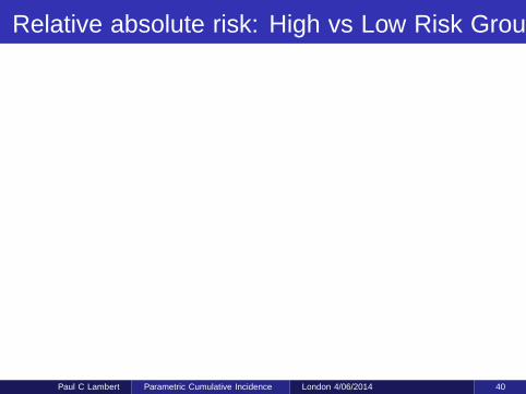
Relative absolute risk: High vs Low Risk Group
1
2
5
10
20
Rel
ativ
e ab
solu
te r
isk
0 1 2 3 4 5Years since transplantation
Paul C Lambert Parametric Cumulative Incidence London 4/06/2014 40
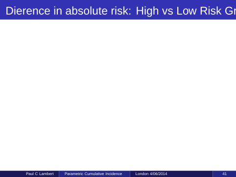
Difference in absolute risk: High vs Low Risk Group
0.00
0.05
0.10
0.15
0.20
0.25D
iffer
ence
in a
bsol
ute
risk
0 1 2 3 4 5Years since transplantation
Paul C Lambert Parametric Cumulative Incidence London 4/06/2014 41

Difference in absolute risk: High vs Low Risk Group
0.00
0.05
0.10
0.15
0.20
0.25D
iffer
ence
in a
bsol
ute
risk
0 1 2 3 4 5Years since transplantation
Paul C Lambert Parametric Cumulative Incidence London 4/06/2014 41
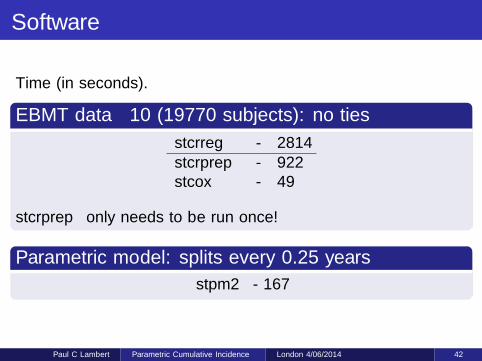
Software
Time (in seconds).
EBMT data ×10 (19770 subjects): no ties
stcrreg - 2814stcrprep - 922stcox - 49
stcrprep only needs to be run once!
Parametric model: splits every 0.25 years
stpm2 - 167
Paul C Lambert Parametric Cumulative Incidence London 4/06/2014 42
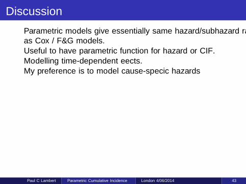
Discussion
Parametric models give essentially same hazard/subhazard ratiosas Cox / F&G models.Useful to have parametric function for hazard or CIF.Modelling time-dependent effects.My preference is to model cause-specific hazards
When modelling CIF, no need to model other competingevent(s).Alternative would be to directly model CIF for all eventtypes[13].Splits for censoring distribution can be fairly crude (importantfor large datasets).Range of link funtions.In flexible parametric models knots choice not crucial.Software available crprep in R and stcrprep in Stata, then usestandard survival methods.
Paul C Lambert Parametric Cumulative Incidence London 4/06/2014 43
Discussion
Parametric models give essentially same hazard/subhazard ratiosas Cox / F&G models.Useful to have parametric function for hazard or CIF.Modelling time-dependent effects.My preference is to model cause-specific hazardsWhen modelling CIF, no need to model other competingevent(s).Alternative would be to directly model CIF for all eventtypes[13].
Splits for censoring distribution can be fairly crude (importantfor large datasets).Range of link funtions.In flexible parametric models knots choice not crucial.Software available crprep in R and stcrprep in Stata, then usestandard survival methods.
Paul C Lambert Parametric Cumulative Incidence London 4/06/2014 43
Discussion
Parametric models give essentially same hazard/subhazard ratiosas Cox / F&G models.Useful to have parametric function for hazard or CIF.Modelling time-dependent effects.My preference is to model cause-specific hazardsWhen modelling CIF, no need to model other competingevent(s).Alternative would be to directly model CIF for all eventtypes[13].Splits for censoring distribution can be fairly crude (importantfor large datasets).Range of link funtions.
In flexible parametric models knots choice not crucial.Software available crprep in R and stcrprep in Stata, then usestandard survival methods.
Paul C Lambert Parametric Cumulative Incidence London 4/06/2014 43
Discussion
Parametric models give essentially same hazard/subhazard ratiosas Cox / F&G models.Useful to have parametric function for hazard or CIF.Modelling time-dependent effects.My preference is to model cause-specific hazardsWhen modelling CIF, no need to model other competingevent(s).Alternative would be to directly model CIF for all eventtypes[13].Splits for censoring distribution can be fairly crude (importantfor large datasets).Range of link funtions.In flexible parametric models knots choice not crucial.Software available crprep in R and stcrprep in Stata, then usestandard survival methods.
Paul C Lambert Parametric Cumulative Incidence London 4/06/2014 43
References
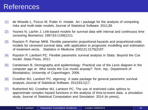
[1] de Wreede L, Fiocco M, Putter H. mstate: An r package for the analysis of competingrisks and multi-state models. Journal of Statistical Software 2011;38.
[2] Younes N, Lachin J. Link-based models for survival data with interval and continuous timecensoring. Biometrics 1997;53:1199–1211.
[3] Royston P, Parmar MKB. Flexible parametric proportional-hazards and proportional-oddsmodels for censored survival data, with application to prognostic modelling and estimationof treatment effects. Statistics in Medicine 2002;21:2175–2197.
[4] Royston P, Lambert PC. Flexible parametric survival analysis in Stata: Beyond the Coxmodel . Stata Press, 2011.
[5] Carstensen B. Demography and epidemiology: Practical use of the Lexis diagram in thecomputer age or: Who needs the Cox model anyway? Tech. rep., Department ofBiostatistics, University of Copenhagen, 2006.
[6] Crowther MJ, Lambert PC. stgenreg: A stata package for general parametric survivalanalysis. Journal of Statistical Software 2013;53:1–17.
[7] Rutherford MJ, Crowther MJ, Lambert PC. The use of restricted cubic splines toapproximate complex hazard functions in the analysis of time-to-event data: a simulationstudy. Journal of Statistical Computation and Simulation 2014 (in press);.
Paul C Lambert Parametric Cumulative Incidence London 4/06/2014 44
References 2
[8] Hinchliffe SR, Lambert PC. Flexible parametric modelling of cause-specific hazards toestimate cumulative incidence functions. BMC Medical Research Methodology 2013;13:13.
[9] Geskus RB. Cause-specific cumulative incidence estimation and the fine and gray modelunder both left truncation and right censoring. Biometrics 2011;67:39–49.
[10] Lambert PC, Royston P. Further development of flexible parametric models for survivalanalysis. The Stata Journal 2009;9:265–290.
[11] Beyersmann J, Latouche A, Buchholz A, Schumacher M. Simulating competing risks datain survival analysis. Stat Med 2009;28:956–971.
[12] Crowther MJ, Lambert PC. Simulating biologically plausible complex survival data.Statistics in Medicine 2013;32:41184134.
[13] Jeong JH, Fine JP. Parametric regression on cumulative incidence function. Biostatistics2007;8:184–196.
Paul C Lambert Parametric Cumulative Incidence London 4/06/2014 45
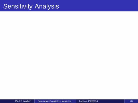
Sensitivity Analysis
0.0
0.1
0.2
0.3
0.4
0.5
Cum
ulat
ive
Inci
denc
e
0 1 2 3 4 5Years since transplantation
df(4) dftvc(3)df(3) dftvc(3)df(5) dftvc(3)df(5) dftvc(4)df(7) dftvc(3)
Paul C Lambert Parametric Cumulative Incidence London 4/06/2014 46


![A COMPARISON OF KAPLAN-MEIER AND CUMULATIVE INCIDENCE ...d-scholarship.pitt.edu/9986/1/BintuSherif_thesis[1].pdf · a comparison of kaplan-meier and cumulative incidence estimate](https://img.pdfslide.us/doc/110x75/5ad1fe937f8b9a92258c90e6/a-comparison-of-kaplan-meier-and-cumulative-incidence-d-1pdfa-comparison-of.jpg)