Main Points to be Covered

• Incidence versus Prevalence

• The 3 elements of measures of incidence

• Cumulative vs. person-time incidence

• Calculating cumulative incidence by the Kaplan-Meier method

• Calculating cumulative incidence by the life table method

Prevalence versus Incidence

• Prevalence counts existing disease diagnoses, often at a single point in time

• Incidence counts new disease diagnoses during a defined time period

Prevalence: 3 types

• Point prevalence - number of existing cases at one point in time divided by population

• Period prevalence - number of existing cases in a time interval (eg, one year) divided by population

• Cumulative (lifetime) prevalence - proportion of people who have had the outcome at any time in the past

The Three Elements in Measures of Disease Incidence

• E = an event = a disease diagnosis or death

• N = number of persons in the population in which the events are observed

• T = time period during which the events are observed

Disease Occurrence Measures: A Confusion of Terms

• Terminology is not standardized and is used carelessly even by those who know better

• Key to understanding measures is to pay attention to how the 3 elements of number of events, number of persons at risk, and time are used

• Even the basic difference between prevalence and incidence is often ignored

HIV/AIDS infection rates drop in Uganda Kyodo News Service KAMPALA, Sept. 10 (Kyodo) - Infection rates of the HIV/AIDS epidemic among Ugandan men, women and children dropped to 6.1% at the end of 2000 from 6.8% a year earlier, an official report shows.

The report, compiled by the Ministry of Health together with the World Health Organization and the Medical Research Council of Britain, says the results were obtained after testing the blood of women attending clinics in 15 hospitals around the country.

The ministry deduced the figures for men and children from the blood tests on women, according to the report.

The report says the average rate of infection for urban areas fell from 10.9% to 8.7%. In rural areas, the average was 4.2%, not much different from the 4.3% average a year earlier. The highest infection rate of 30% was last reported in western Uganda in 1992.

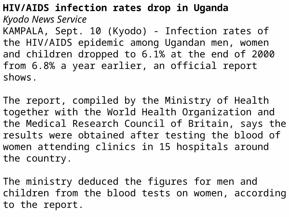
The word “rate” should be avoided when existing cases at one point in time are what was measured.

Although you may encounter “prevalencerate,” rate should be reserved formeasuring incidence.

In general a rate is a change in onemeasure with respect to change in a 2nd

Measures that are sometimes loosely called Incidence

• Count of the number of events (E)– eg, there were 84 traffic fatalities during the

holidays

• Count of the number of events during some time period (E/T)– eg, traffic accidents have averaged 50 per week

during the past year

• Neither explicitly includes the number of persons (N) giving rise to the events

Two Measures Described as Incidence in the Text

• The proportion of individuals who experience the event in a defined time period (E/N during some time T) = cumulative incidence

• The number of events divided by the amount of person-time observed (E/NT) = incidence rate or density (not a proportion)

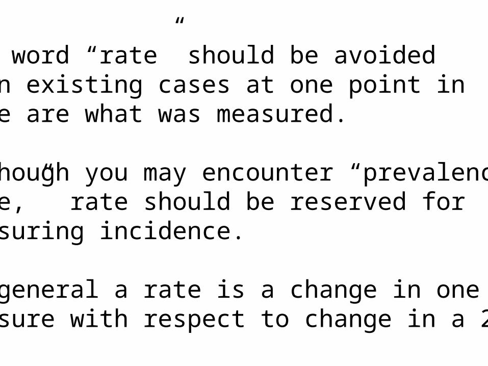
E E/T E/NT E/N

Cumulative Incidence

• Perhaps most intuitive measure of incidence since it is just proportion of those observed who got the disease

• Proportion=probability=risk

• Basis for Survival Analysis

• Two primary methods for calculating– Kaplan-Meier method– Life table method

Survival Analysis• Data analysis for which the outcome is

time to an event• The time variable is usually called survival time• The outcome event is usually called a failure

(normally an adverse event but it doesn’t have to be)

• Cumulative incidence is the complement of cumulative survival (1 - cumulative survival)

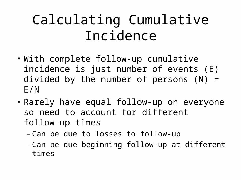
Calculating Cumulative Incidence

• With complete follow-up cumulative incidence is just number of events (E) divided by the number of persons (N) = E/N

• Rarely have equal follow-up on everyone so need to account for different follow-up times – Can be due to losses to follow-up – Can be due beginning follow-up at different times

Cumulative Incidence in the Setting of a Cohort Study

If number of events (E) for all 1000 is known, cumulativeincidence is just E/1000. But 7 persons left the cohort.

Cumulative incidence with Kaplan-Meier estimate

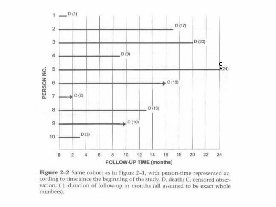
• Set in a cohort– subjects have different starting dates

– subjects have different amounts of follow-up time

• Requires date last observed or date outcome occurred on each individual (end of study can be the last date observed)

• Analysis is performed by dividing the follow-up time into discrete pieces– calculate probability of survival at each event

3 Ways Censoring Occurs1) Death (if death is not the study outcome)

2) Loss to follow-up (refuse, move, can’t be found)

3) End of study observation (if still alive and haven’t experienced outcome)

• Each subject either experiences the outcome or is censored in a survival analysis

c

Calculating Cumulative Incidence

• Probability of two independent events occurring is the product of the two probabilities for each occurring alone– eg, if event 1 occurs with probability 1/6 and event 2 with

probability 1/2, then the probability of both event 1 and 2 occurring = 1/6 x 1/2 = 1/12

• Conditional probability of living to time 2 given that one has already lived to time 1 is independent of the probability of living to time 1

Cumulative calculated by multiplying probabilities for each prior failure time: e.g., 0.9 x 0.875 x 0.857 = 0.675 and0.9 x 0.875 x 0.857 x 0.800 x 0.667 x 0.500 = 0.180

Graphical representation of K-M survival analysis (survival curve with discrete steps)

Kaplan-Meier Cumulative Incidence of the Outcome

• Cannot calculate by multiplying each event probability (=probability of repeating event) – (in our example, 0.100 x 0.125 x 0.143 x 0.200 x 0.333 x

0.500 = 0.0000595)

• Obtain by subtracting cumulative probability of surviving from 1; eg, (1 - 0.180) = 0.82

• Since it is a proportion, it has no time unit connected to it, so time period has to be added; e.g, 2-year cumulative incidence

Kaplan-Meier using STATA

Need a data set with one observation per person.

Each person either experiences event or is censored.

Need a variable for the time from study entry to date of event or date of censoring (time variable=timevar).

Need a variable indicating whether follow-up ended with the event or with censoring (failure variable=failvar)

USING STATA TO RUN KAPLAN MEIERSURVIVAL ANALYSIS

TYPE IN COMMAND WINDOW AFTER OPENINGSTATA.

POINT TO DIRECTORY OF DATA SET TO BE USED.

. cd C:\pathofdirectory

(note: don't type the initial period)

SELECT AND OPEN THE DATA SET TO BE USED.

. use datasetname, clear

TO DO SURVIVAL ANALYSIS (KAPLAN-MEIER, RATES, ETC)NEED TO DECLARE DATA SET SURVIVAL DATA.

. stset time, fail(d)

failure event: d ~= 0 & d ~= .obs. time interval: (0, time]exit on or before: ailure

------------------------------------------------------------------------------ 184 total obs. 0 exclusions------------------------------------------------------------------------------ 184 obs. remaining, representing 96 failures in single record/single failure data 747.039 total analysis time at risk, at risk from t = 0 earliest observed entry t = 0 last observed exit t = 11.64408

TO OBTAIN KAPLAN-MEIER ESTIMATES OF SURVIVAL: . sts list failure _d: d analysis time _t: time Time Beg. Net Survivor

Total Fail Lost Function [95% C.I.] .0219 184 0 1 1.0000 . . .0246 183 2 0 0.9891 0.957 0.997 .052 181 1 0 0.9836 0.950 0.994 . . . . . . . . . . . . . . . . . . . . 9.5 6 0 1 0.2375 0.144 0.344 10.14 5 0 1 0.2375 0.144 0.343

TO GRAPH A CURVE FROM THE KAPLAN-MEIER ESTIMATES:

. sts graphKaplan-Meier survival estimate

analysis time0 5 10 15

0.00

0.25

0.50

0.75

1.00

Two assumptions in survival analysis

• Censoring is unrelated to survival (unrelated to the probability of experiencing the outcome)

• There are no temporal trends in the probability of the outcome

Life table method of estimating cumulative incidence

• Key difference from Kaplan-Meier is that probabilities are calculated for fixed time intervals, not at the exact time of each event

• Fixed time intervals can vary in length but are often uniform

• Probability of surviving each fixed time interval is calculated

• Cumulative survival is product of probabilities from each prior time period

Life table method of estimating cumulative incidence

• Since exact event times not used, assumption that events and censoring occur uniformly during the fixed time intervals

• Calculations are based on assigning censored individuals follow-up for half of the time period (follows from uniformity assumption)

• Subtract one-half of subjects lost during interval from denominator at interval beginning

c

6 deaths in 2 years;3 censoredbefore 2years offollow-up

Example of Life Table Calculation from the Text Data

Taking the full 2-year period as one interval:

6 deaths in the numerator and 10 (initial number) minus0.5 x 3 censored persons in the denominator = 6 / 8.5 = 0.71, the cumulative probability of death

(1 - 0.71) = 0.29, the cumulative probability of survival(NB - text gives this incorrectly as 0.39)

Note this differs from the Kaplan-Meier cumulativesurvival estimate of 0.18

Example of Life Table Calculation Using Two One-Year Intervals

Taking two 1-year time intervals:

First year: Starts with 10 at risk, 3 deaths, 2 censored, probability of survival is 7 / 10 - 0.5 x 2 = 7/9 = 0.777

Second year: Starts with 5 at risk, 3 deaths, 1 censored,probability of survival is 2 / 5 - 0.5 x 1 = 2/4.5 = 0.444

Cumulative probability of survival = 0.777 x 0.444 = 0.345

This differs from both the Kaplan-Meier estimate and the life table using only one 2-year interval.

Life Table Method

• Can see from inspecting the data used in the text that for these 10 observations the life table uniformity assumption doesn’t hold

• Life table more commonly used on large secondary data sets where information on exact failure times are not available

• With very large numbers the uniformity assumption is more likely to be valid

Life Table of Breast Ca Survival

Yearobser Alive Died

Leftcohort

N atrisk

Prop.dying

Cum.Surv.

0-1 840 93 4 838.0 0.111 0.889

1-2 743 93 63 711.5 0.131 0.773

2-3 587 55 67 554.5 0.099 0.696

3-4 465 55 42 445.0 0.124 0.610

4-5 368 25 32 353.0 0.071 0.567

Summary Points• Prevalence counts existing cases and incidence counts new

cases• Word “rate” is very loosely used• Two main types of incidence rate

– incidence based on proportion of persons– incidence based on person-time

• Kaplan-Meier or life table method of estimating cumulative incidence assume losses unrelated to outcome probability and that there are no temporal trends in outcome probability