Embed Size (px)
Citation preview

Estimating and modelling cumulative incidence
functions using time-dependent weights
Paul C Lambert1,2
1Department of Health Sciences, University of Leicester, Leicester, UK2Department of Medical Epidemiology and Biostatistics,
Karolinska Institutet, Stockholm, Sweden
UK Stata Users Group, London, September 2013
Paul Lambert Cumulative Incidence Functions UKSUG 2013 1/32
Competing Risks
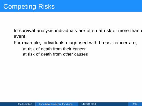
In survival analysis individuals are often at risk of more than oneevent.
For example, individuals diagnosed with breast cancer are,
at risk of death from their cancerat risk of death from other causes
The probability of dying from cancer will depend upon themortality rate due to cancer and the mortality rate due to othercauses.
This is a classic competing risks situation.
Paul Lambert Cumulative Incidence Functions UKSUG 2013 2/32

Competing Risks
In survival analysis individuals are often at risk of more than oneevent.
For example, individuals diagnosed with breast cancer are,
at risk of death from their cancerat risk of death from other causes
The probability of dying from cancer will depend upon themortality rate due to cancer and the mortality rate due to othercauses.
This is a classic competing risks situation.
Paul Lambert Cumulative Incidence Functions UKSUG 2013 2/32

Competing risks schematic
Alive
Cancer
CVD
Other
h1(t)
h2(t)
h3(t)
Paul Lambert Cumulative Incidence Functions UKSUG 2013 3/32

Cause specific hazard function
For cause k ,
hk(t) = limδ→0
P (t ≤ T < t + δ, event = k |T > t)
δ
To still be at risk at time t a subject can not have died of causek or any of the K − 1 other causes.
Total hazard (mortality) rate
h(t) =K∑
k=1
hk(t)
All cause survival
S(t) = exp
(−∫ t
0
h(u)du
)= exp
(−∫ t
0
K∑k=1
hk(u)du
)Paul Lambert Cumulative Incidence Functions UKSUG 2013 4/32

Cause specific cumulative incidence function
We want the probability of dying of cause k accounting for thecompeting risks.For cause k .
CIFk(t) = P (T ≤ t, event = k)
CIFk(t) =
∫ t
0
S(u)hk(u)du
CIF (t) =K∑
k=1
CIFk(t)
Note: CIF does not require independence between causes.For further details on competing risks see references [1, 2, 3]Post estimation command stpm2cif will estimate CIFs andrelated measures after using stpm2 to model cause-specifichazards [4, 5]
Paul Lambert Cumulative Incidence Functions UKSUG 2013 5/32
Key Paper: Geskus 2011[8]
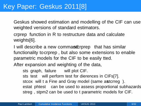
Geskus showed estimation and modelling of the CIF can useweighted versions of standard estimators.
crprep function in R to restructure data and calculateweights[6].
I will describe a new command stcrprep that has similarfunctionality to crprep, but also some extensions to enableparametric models for the CIF to be easily fitted.
After expansion and weighting of the data,
sts graph, failure will plot CIF.sts test will perform test for differences in CIFs[7].stcox will fit a Fine and Gray model (same as stcrreg).estat phtest can be used to assess proportional subhazards.streg, stpm2 can be used to fit parametric models for CIF.
Paul Lambert Cumulative Incidence Functions UKSUG 2013 6/32

Data expansion and weighting
Define event of interest.
Subjects that have a competing event are kept in the risk set tothe end of follow-up.
However, there is a a chance that they would be censored aftertheir competing event.
Estimate censoring distribution.
Weights depend on conditional probability of not being censoredafter competing event.
Paul Lambert Cumulative Incidence Functions UKSUG 2013 7/32
Data Expansion for Competing Events
9
8
7
6
5
4
3
2
1
Time
Censored Cancer Other
Paul Lambert Cumulative Incidence Functions UKSUG 2013 8/32

Data Expansion for Competing Events
9
8
7
6
5
4
3
2
1
Time
Censored Cancer Other
Paul Lambert Cumulative Incidence Functions UKSUG 2013 8/32

Data Expansion for Competing Events
w81 w82 w83 w84
w41 w42
9
8
7
6
5
4
3
2
1
Time
Censored Cancer Other
Paul Lambert Cumulative Incidence Functions UKSUG 2013 8/32

Data Expansion for Competing Events
w81 w82 w83 w84
w41 w42
9
8
7
6
5
4
3
2
1
Time
Censored Cancer Other
Paul Lambert Cumulative Incidence Functions UKSUG 2013 8/32

Initial data
Competing event: d == 2
. stset t, failure(d==1,2) id(id)(output omitted )
. list id d _t0 _t _d, noobs sep(0)
id d _t0 _t _d
1 1 0 3.5 12 2 0 2 13 1 0 5 14 2 0 5.5 15 0 0 3.5 06 1 0 6 17 1 0 8 18 0 0 6.5 09 0 0 7.5 0
Paul Lambert Cumulative Incidence Functions UKSUG 2013 9/32

Using stcrprep
Competing event: d == 2
. stcrprep, events(d) trans(1) noshorten
. gen event = d == failcode
. stset tstop [iw = weight_c], failure(event) enter(tstart) id(id)(output omitted )
. list id d _t0 _t _d weight_c, noobs sep(0)
id d _t0 _t _d weight_c
1 1 0 3.5 1 12 2 0 2 0 12 2 2 3.5 0 12 2 3.5 5 0 .857142862 2 5 6 0 .857142862 2 6 8 0 .285714293 1 0 5 1 14 2 0 5.5 0 14 2 5.5 6 0 14 2 6 8 0 .333333335 0 0 3.5 0 16 1 0 6 1 17 1 0 8 1 18 0 0 6.5 0 19 0 0 7.5 0 1
Paul Lambert Cumulative Incidence Functions UKSUG 2013 10/32

European Blood and Marrow Transplantation Data
1977 patients from the European Blood and MarrowTransplantation (EBMT) registry who received an allogeneicbone marrow transplantation[6].
Events are death and relapse
836 censored456 relapse685 died
One covariate of interest, the EBMT risk score, which has beencategorized into 3 groups (low, medium and high risk).
Paul Lambert Cumulative Incidence Functions UKSUG 2013 11/32

Using stcrprep
stcrprep
. stset time, failure(status==1,2) scale(365.25) id(patid)(output omitted )
. stcrprep, events(status) keep(score) trans(1 2) byg(score)
. gen event = status == failcode
. stset tstop [iw=weight_c], failure(event=1) enter(tstart) noshow(output omitted )
We can now estimate the CIF using sts graph.
sts graph
. sts graph if failcode == 1, by(score) failure // relapse
. sts graph if failcode == 2, by(score) failure // death
Paul Lambert Cumulative Incidence Functions UKSUG 2013 12/32

Using sts graph to estimate cause-specific CIF
0.0
0.1
0.2
0.3
0.4
0.5
Pro
babi
lity
of R
elap
se
0 2 4 6 8Years since transplanation
Low RiskMedium RiskHigh Risk
Kaplan-Meier failure estimates
Paul Lambert Cumulative Incidence Functions UKSUG 2013 13/32

Testing for difference between cause-specific CIFs
Use sts test
sts test
. sts test score if failcode == 1
Log-rank test for equality of survivor functions
Events Eventsscore observed expected
Low risk 79 98.77Medium risk 328 322.61High risk 49 34.62
Total 456 456.00
chi2(2) = 10.03Pr>chi2 = 0.0067
Similar to Gray’s test [7] since the number at risk is modifiedwhen compared to the standard log-rank test.
Paul Lambert Cumulative Incidence Functions UKSUG 2013 14/32

Using stcox to fit Fine and Gray Model[9]Use stcrprep without byg() option since Fine and Gray modelassumes common censoring distribution.
. stcrprep, events(status) keep(score) trans(1 2)
. stset tstop [iw=weight c], failure(event) enter(tstart)
stcox
. stcox i.score if failcode == 1, nologCox regression -- Breslow method for tiesNo. of subjects = 72880.46857 Number of obs = 72880No. of failures = 456Time at risk = 6026.27434
LR chi2(2) = 9.63Log likelihood = -3333.3112 Prob > chi2 = 0.0081
_t Haz. Ratio Std. Err. z P>|z| [95% Conf. Interval]
scoreMedium risk 1.271235 .1593392 1.91 0.056 .9943389 1.625238
High risk 1.769899 .3219273 3.14 0.002 1.239148 2.52798
Paul Lambert Cumulative Incidence Functions UKSUG 2013 15/32

Comparison with stcrreg
Comparison of Estimates
. estimates table stcrreg stcox*, eq(1) b(%6.5f) se(%6.5f) modelwidth(12)
Variable stcrreg stcox stcox_robust
scoreMedium risk 0.23998 0.23999 0.23999
0.12227 0.11861 0.12225High risk 0.57090 0.57092 0.57092
0.18298 0.16941 0.18297
legend: b/se
Use pweights and vce(cluster id) for robust standarderrors.However, Geskus (2011) showed that robust standard errors areless efficient[8].
Perhaps stcrreg should have a ‘norobust’ option.
Paul Lambert Cumulative Incidence Functions UKSUG 2013 16/32

Comparison with stcrreg
Comparison of Estimates
. estimates table stcrreg stcox*, eq(1) b(%6.5f) se(%6.5f) modelwidth(12)
Variable stcrreg stcox stcox_robust
scoreMedium risk 0.23998 0.23999 0.23999
0.12227 0.11861 0.12225High risk 0.57090 0.57092 0.57092
0.18298 0.16941 0.18297
legend: b/se
Use pweights and vce(cluster id) for robust standarderrors.However, Geskus (2011) showed that robust standard errors areless efficient[8].Perhaps stcrreg should have a ‘norobust’ option.
Paul Lambert Cumulative Incidence Functions UKSUG 2013 16/32

Time Improvements (seconds)
EBMT data (1977 subjects)
stcrreg - 18.2stcrprep - 14.3stcox - 1.5
stcrprep only needs to be run once!
EBMT data ×10 (19770 subjects): no ties
stcrreg - 2814stcrprep - 922stcox - 49
stcrprep only needs to be run once!
Paul Lambert Cumulative Incidence Functions UKSUG 2013 17/32

Proportional subhazards (estat phtest)
Assess proportional subhazards using Schoenfeld residuals.
. estat phtest,Test of proportional-hazards assumptionTime: Time
chi2 df Prob>chi2
global test 23.24 2 0.0000
.5
11.5
5
10
Exp
onen
tiate
d sc
aled
Sch
oenf
eld
resi
dual
0 1 2 3 4Years since transplanation
Schoenfeld Residuals for High Risk Group
Paul Lambert Cumulative Incidence Functions UKSUG 2013 18/32

Proportional subhazards (estat phtest)
Assess proportional subhazards using Schoenfeld residuals.. estat phtest,
Test of proportional-hazards assumptionTime: Time
chi2 df Prob>chi2
global test 23.24 2 0.0000
.5
11.5
5
10
Exp
onen
tiate
d sc
aled
Sch
oenf
eld
resi
dual
0 1 2 3 4Years since transplanation
Schoenfeld Residuals for High Risk Group
Paul Lambert Cumulative Incidence Functions UKSUG 2013 18/32
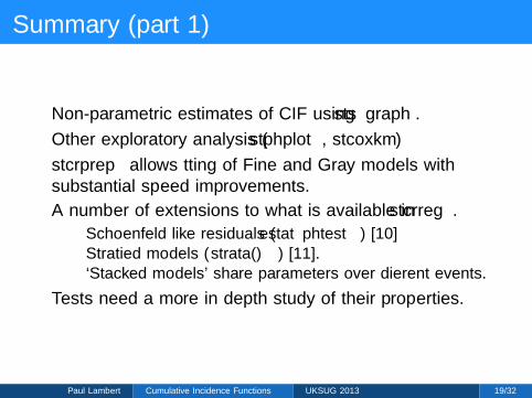
Summary (part 1)
Non-parametric estimates of CIF using sts graph.
Other exploratory analysis (stphplot, stcoxkm)
stcrprep allows fitting of Fine and Gray models withsubstantial speed improvements.
A number of extensions to what is available in stcrreg.
Schoenfeld like residuals (estat phtest) [10]Stratified models (strata()) [11].‘Stacked models’ share parameters over different events.
Tests need a more in depth study of their properties.
Paul Lambert Cumulative Incidence Functions UKSUG 2013 19/32
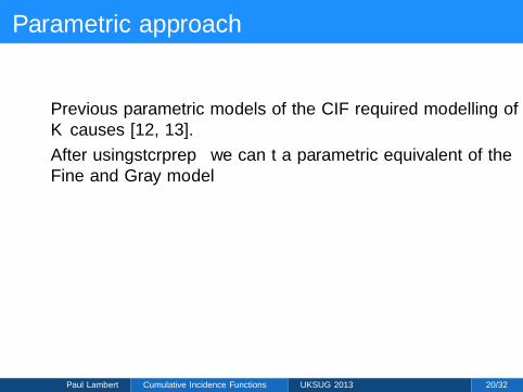
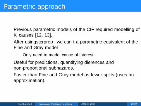
Parametric approach
Previous parametric models of the CIF required modelling of allK causes [12, 13].
After using stcrprep we can fit a parametric equivalent of theFine and Gray model
Only need to model cause of interest.
Useful for predictions, quantifying differences andnon-proportional subhazards.
Faster than Fine and Gray model as fewer splits (uses anapproximation).
Paul Lambert Cumulative Incidence Functions UKSUG 2013 20/32

Parametric approach
For those with competing events, allow to be at risk to end ofpotential follow-up.Split follow-up after competing event into (small) time-intervals.Apply weights to each interval.
Likelihood
ln Li = d1i ln [h1(ti)] + (1− d2i) ln [S(ti)] +
d2i
Ji∑j=1
wij
(ln [S(tij)]− ln
[S(ti(j−1))
])Need to specify parametric form of CIF for event of interest, butnot for competing events.Also need weighting function. Obtained by modelling censoringdistribution.
Paul Lambert Cumulative Incidence Functions UKSUG 2013 21/32

Splitting
Censored
Event 2
Event 1
Time
Paul Lambert Cumulative Incidence Functions UKSUG 2013 22/32

Splitting
Censored
Event 2
Event 1
Time
Paul Lambert Cumulative Incidence Functions UKSUG 2013 22/32

Splitting
Censored
Event 2
Event 1
Time
Paul Lambert Cumulative Incidence Functions UKSUG 2013 22/32

Splitting
w1 w2 w3 w4 w5
Censored
Event 2
Event 1
Time
Paul Lambert Cumulative Incidence Functions UKSUG 2013 22/32

The censoring distribution
Fit a parametric model stpm2,
Option to include a variety of covariates.Also to model time-dependent effects.
stcrreg assumes common censoring distribution.
Need to decide where to evaluate censoring distribution (numberof split points) for weighted likelihood.
Paul Lambert Cumulative Incidence Functions UKSUG 2013 23/32

Flexible parametric models
Possible to use any parametric approach that allows for delayedentry and weights.
We use flexible parametric survival models that uses restrictedsplines to model the baseline using stpm2 in Stata. [14, 15].
g [S(t|xi)] = ηi = s (ln(t)|γ, k0) + xiβ
where s (ln(t)|γ, k0) is a restricted cubic spline function of ln(t)with knots, k0.
g() is a link function.
Paul Lambert Cumulative Incidence Functions UKSUG 2013 24/32

Link Functions
When using weights with expanded data
proportional sub hazards
log(− log (1− CIFk(t|xi))) = s (ln(t)|γ, k0) + xiβ
proportional odds
log
(CIFk(t|xi)
1− CIFk(t|xi)
)= s (ln(t)|γ, k0) + xiβ
relative absolute risk
log (CIFk(t|xi)) = s (ln(t)|γ, k0) + xiβ
Time-dependent effects can be fitted for any of these linkfunctions.
Paul Lambert Cumulative Incidence Functions UKSUG 2013 25/32

Parametric proportional subhazards models 1
stcrprep
. stset time, failure(status==1,2) scale(365.25) id(patid)(output omitted )
. stcrprep, events(status) keep(score) trans(1 2) censstpm2 every(0.2)
. gen event = status == failcode
. stset tstop [iw=weight_c], failure(event) enter(tstart) noshowfailure event: event != 0 & event < .
obs. time interval: (0, tstop]enter on or after: time tstartexit on or before: failure
weight: [iweight=weight_c]
48116 total observations0 exclusions
48116 observations remaining, representing1141 failures in single-record/single-failure data
16367.15 total analysis time at risk and under observationat risk from t = 0
earliest observed entry t = 0last observed exit t = 8.454483
Paul Lambert Cumulative Incidence Functions UKSUG 2013 26/32
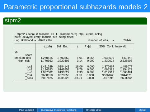
Parametric proportional subhazards models 2
stpm2
. stpm2 i.score if failcode == 1, scale(hazard) df(4) eform nolognote: delayed entry models are being fittedLog likelihood = -1678.7162 Number of obs = 29147
exp(b) Std. Err. z P>|z| [95% Conf. Interval]
xbscore
Medium risk 1.270615 .1592552 1.91 0.056 .9938639 1.62443High risk 1.770563 .3220405 3.14 0.002 1.239624 2.528908
_rcs1 1.431289 .0284143 18.06 0.000 1.376667 1.488077_rcs2 1.124393 .0149958 8.79 0.000 1.095382 1.154172_rcs3 1.037582 .0130522 2.93 0.003 1.012313 1.063481_rcs4 .9688918 .0078559 -3.90 0.000 .9536162 .9844121_cons .2087425 .0235126 -13.91 0.000 .167391 .2603092
Sub-hazard ratios very similar to semi-parametric estimates.
Paul Lambert Cumulative Incidence Functions UKSUG 2013 27/32

Predictions of CIF
predict cif, failure
0.0
0.1
0.2
0.3
0.4
0.5
Pro
babi
lity
of R
elap
se
0 2 4 6 8Years since transplanation
Proportional subhazards
0.0
0.1
0.2
0.3
0.4
0.5
Pro
babi
lity
of R
elap
se
0 2 4 6 8Years since transplanation
Low Risk
Medium Risk
High Risk
Non-proportional subhazards
Paul Lambert Cumulative Incidence Functions UKSUG 2013 28/32

Difference in CIFs
. predict CIF diff, sdiff1(score2 0 score3 0) sdiff2(score3 1) ci
0.00
0.05
0.10
0.15
0.20
0.25
0.30
Diff
eren
ce in
Pro
babi
lity
of R
elap
se
0 1 2 3 4 5Years since transplanation
Take reciprocal to estimate Number Needed to Treat (NNT)accounting for competing risks[16]
Paul Lambert Cumulative Incidence Functions UKSUG 2013 29/32

Relative absolute risks
stpm2
. stpm2 i.score if failcode == 1, scale(log) df(4) eform nolognote: delayed entry models are being fittedLog likelihood = -1680.1742 Number of obs = 29147
exp(b) Std. Err. z P>|z| [95% Conf. Interval]
xbscore
Medium risk 1.19893 .1332627 1.63 0.103 .9642325 1.490755High risk 1.543556 .2392695 2.80 0.005 1.139137 2.091553
_rcs1 1.38459 .0247152 18.23 0.000 1.336987 1.433889_rcs2 1.126424 .0141052 9.51 0.000 1.099115 1.154412_rcs3 1.034958 .0127994 2.78 0.005 1.010174 1.060351_rcs4 .9702326 .0072774 -4.03 0.000 .9560736 .9846014_cons .1922568 .0193746 -16.36 0.000 .1577982 .2342401
Effect sizes are now relative risks rather than subhazard ratios.Assumed constant over time, but this can be relaxed.
Paul Lambert Cumulative Incidence Functions UKSUG 2013 30/32

Summary (part 2)
Parametric version of Fine and Gray model.
Only need to model event of interest to estimate CIF.
Models on a variety of scales.
Can relax the proportionality assumption.
Need to choose split times, but can be fairly crude.
When modelling competing risks, still useful to modelcause-specific hazards.
See stpm2cif[5]
Paul Lambert Cumulative Incidence Functions UKSUG 2013 31/32
References[1] Andersen PK, Abildstrom SZ, Rosthøj S. Competing risks as a multi-state model. Stat
Methods Med Res 2002;11:203–215.
[2] Coviello V, Boggess M. Cumulative incidence estimation in the presence of competingrisks. The Stata Journal 2004;4:103–112.
[3] Putter H, Fiocco M, Geskus RB. Tutorial in biostatistics: competing risks and multi-statemodels. Statistics in Medicine 2007;26:2389–2430.
[4] Hinchliffe SR, Lambert P. Flexible parametric modelling of cause-specific hazards toestimate cumulative incidence functions. BMC Medical Research Methodology 2013;13:13.
[5] Hinchliffe SR, Lambert P. Extending the flexible parametric survival model for competingrisks. The Stata Journal 2013;13:344–355.
[6] de Wreede L, Fiocco M, Putter H. mstate: An r package for the analysis of competingrisks and multi-state models. Journal of Statistical Software 2011;38.
[7] Gray R. A class of k-sample tests for comparing the cumulative incidence of a competingrisk. The Annals of Statistics 1988;16:1141–1154.
[8] Geskus RB. Cause-specific cumulative incidence estimation and the fine and gray modelunder both left truncation and right censoring. Biometrics 2011;67:39–49.
[9] Fine JP, Gray RJ. A proportional hazards model for the subdistribution of a competingrisk. Journal of the American Statistical Association 1999;446:496–509.
[10] Zhou B, Fine J, Laird G. Goodness-of-fit test for proportional subdistribution hazardsmodel. Stat Med 2013;.
[11] Zhou B, Latouche A, Rocha V, Fine J. Competing risks regression for stratified data.Biometrics 2011;67:661–670.
[12] Jeong JH, Fine JP. Parametric regression on cumulative incidence function. Biostatistics2007;8:184–196.
[13] Jeong JH, Fine JP. Direct parametric inference for the cumulative incidence function.Applied Statistics 2006;55:187–200.
[14] Lambert PC, Royston P. Further development of flexible parametric models for survivalanalysis. The Stata Journal 2009;9:265–290.
[15] Royston P, Lambert PC. Flexible parametric survival analysis in Stata: Beyond the Coxmodel . Stata Press, 2011.
[16] Gouskova NA, Kundu S, Imreyb PB, Fine JP. Number needed to treat for time-to-eventdata with competing risks. Statistics in Medicine 2013;(in press).
Paul Lambert Cumulative Incidence Functions UKSUG 2013 32/32