Instructions for use

Title Parameter tuning in the support vector machine and random forest and their performances in cross- and same-year cropclassification using TerraSAR-X

Author(s) Sonobe, Rei; Tani, Hiroshi; Wang, Xiufeng; Kobayashi, Nobuyuki; Shimamura, Hideki

Citation International Journal of Remote Sensing, 35(23): 7898-7909

Issue Date 2014-11

Doc URL http://hdl.handle.net/2115/60345

Rights This is an Accepted Manuscript of an article published by Taylor & Francis in International Journal of Remote Sensingon 2014, available online: http://www.tandfonline.com/10.1080/01431161.2014.978038

Type article (author version)

File Information manuscript_IJRS-2014.pdf

Hokkaido University Collection of Scholarly and Academic Papers : HUSCAP

1

Parameter tuning in the support vector machine and random forest 1

and their performances in cross- and same-year crop classification 2

using TerraSAR-X 3

Rei Sonobe*a, Hiroshi Tanib, Xiufeng Wangb, Nobuyuki Kobayashic and 4

Hideki Shimamurad 5

a JSPS Research Fellow / Graduate School of Agriculture. Hokkaido University, 6

Sapporo, Hokkaido 060-8589, Japan 7

b Research Faculty of Agriculture. Hokkaido University, Sapporo, Hokkaido 060-8589, 8

Japan 9

c Smart Link Hokkaido, Iwamizawa, Hokkaido 068-0034, Japan 10

d PASCO Corporation, Meguro-Ku, Tokyo 153-0043, Japan 11

12

Corresponding author 13

Kita 9, Nishi 9 Kita-ku, Sapporo, 060-8589, Japan 14

reysnb@gmail.com 15

16

2

Parameter tuning in the support vector machine and random forest 1

and their performances in cross- and same-year crop classification 2

using TerraSAR-X 3

This paper describes the comparison of three different classification algorithms 4

for mapping crops in Hokkaido, Japan, using TerraSAR-X data. In the study area, 5

beans, beets, grasslands, maize, potatoes and winter wheat were cultivated. 6

Although classification maps are required for management and for the estimation 7

of agricultural disaster compensation, those techniques have yet to be established. 8

Some supervised learning models may allow accurate classification. Therefore, 9

comparisons among the classification and regression tree (CART), the support 10

vector machine (SVM) and the random forests (RF) were performed. SVM was 11

the best algorithm in this study, achieving overall accuracies of 89.1% for the 12

same-year classification, which is the classification using the training data in 13

2009 to classify the test data in 2009, and 78.0% for the cross-year classification, 14

which is the classification using the training data in 2009 to classify the data in 15

2012. 16

1. Introduction 17

Land-cover classification is one of the most common applications of remote sensing. 18

Crop type classification maps are useful for estimating the amount of crops harvested or 19

agricultural disaster compensation. Furthermore, the ability to generate crop type 20

classification maps without concurrent training data is useful for reducing labour costs 21

for the management of the agricultural field and early information gathering. Optical 22

remote sensing is still one of the most attractive options for obtaining biomass 23

information, and new sensors are available with fine spatial and spectral resolutions 24

(Sarker and Nichol 2011). In addition, some optical satellites, such as Landsat, have 25

been used for crop type classification (Hartfield et al. 2013; Mishra and Crews 2014). 26

Significant information about soil and vegetation parameters has also been obtained 27

through microwave remote sensing, and these techniques are increasingly being used to 28

3

manage land and water resources for agricultural applications (Fontanelli et al. 2013). 1

Unlike passive systems, synthetic aperture radar (SAR) systems are not dependent on 2

atmospheric influences or weather conditions; thus, they are especially suitable for a 3

multi-temporal classification approaches (Bargiel and Herrmann 2011). The number of 4

studies on rice monitoring and mapping using SAR data has increased, and there are 5

strong correlations between the backscattering coefficients and the plant height and age. 6

There are examples of uses for crop growth monitoring of beets (Vyas et al. 2003), 7

maize (Beriaux et al. 2013; Blaes et al. 2006), and wheat (Fontanelli et al. 2013; 8

Lievens and Verhoest 2011; Mattia et al. 2003; Sonobe et al. 2014c). Furthermore, SAR 9

data have been used to identify specific crop types, such as paddy fields (Choudhury 10

and Chakraborty 2006; Kuenzer and Knauer 2013). The basic idea of these studies is to 11

use multi-temporal SAR data within a vegetation period to clarify the change pattern 12

with the time series (Costa, 2004), and it may be applied for other crop types. The 13

backscattering coefficient is a function of the geometry and dielectric properties of the 14

target and the amount of biomass in agricultural fields. Therefore, different types of 15

temporal changes can be distinguished with multi-temporal SAR data. The first large 16

backscatter intensity change occurs as a result of ploughing and seeding. Smaller 17

changes occur due to variations of biomass and plant water content, and, for X-band 18

SAR data, changes in the plant structure. Furthermore, harvesting causes large 19

backscatter intensity changes (Blaes and Defourny 2003; Sonobe et al. 2014a). 20

Sometimes, however, no backscatter intensity change is observed despite geometric 21

changes. This is typically observed for dense vegetation, such as grasslands, for high 22

frequency SAR data, such as C-band (Blaes and Defourny 2003). This indicates the 23

potential of the discrimination between gramineous crops (grass and wheat in this 24

study) and others. Sonobe et al. (2014b) shows the potential of X-band SAR data for 25

4

mapping winter-wheat planted areas by Otsu’s method (Otsu, 1979). 1

SAR signals acquired under different polarisations show different backscatter 2

responses, providing more information about vegetation (Brisco et al. 2013) There is a 3

combination of SAR frequencies, polarisations, and incidence angles that is most 4

suitable for best retrieving soil and vegetation parameters (Ulaby et al. 1986). 5

Multi-temporal dual polarimetric (HH/VV) TerraSAR-X data acquired in 6

StripMap mode were obtained, and the resolutions were 2.75 m in the enhanced 7

ellipsoid corrected format. TerraSAR-X was launched on June 15, 2007, and X-band 8

SAR data are widely available and often operated with dual polarisations. Furthermore, 9

previous studies have proven the high geometric accuracy of TerraSAR-X (Ager and 10

Bresnahan 2009). The robustness of the multi-temporal classification approach with 11

high-resolution TerraSAR-X spotlight data was also shown for a same year 12

classification (Bargiel and Herrmann 2011). However, in order to reduce the labour 13

costs for the selection of training data, which are sometimes collected by in situ surveys, 14

the use of training data selected in another year should be considered. 15

Within this framework, the main objectives of the present study are to evaluate 16

the potential of Terra-SAR-X data for crop type classification and crop map generation 17

without concurrent training data. 18

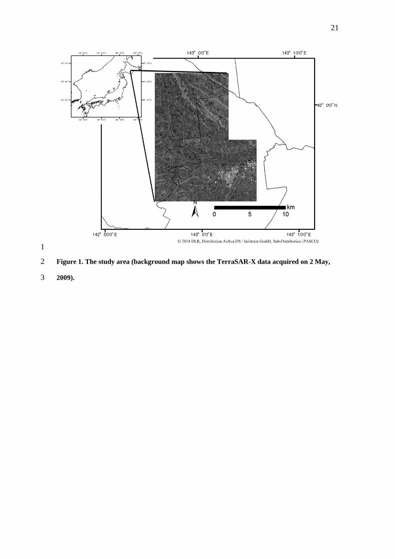
2. Study Area 19

The experimental area of this study (Figure 1) is the farming area in western Tokachi 20

plain, Hokkaido, Japan (142°55′12″ to 143°05′51″E, 42°52′48″ to 43°02′42″N) at an 21

elevation between 50 and 230 m. The climate of the study area is characterised by warm 22

summers and cold winters with an average annual temperature of 6°C and annual 23

precipitation of 920 mm. 24

5

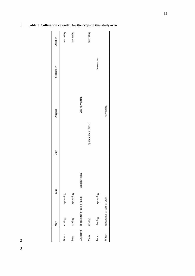
The dominant crops are beans (azuki and soy), beets, grasslands, maize (dent corn and 1

sweet corn), potatoes and winter wheat. A total of 4,955 fields (1,053 beans fields, 709 2

beet fields, 623 grasslands, 254 maize fields, 831 potato fields and 1,485 winter wheat 3

fields) covered the area in 2009, and 5,074 fields (960 bean fields, 625 beet fields, 644 4

grasslands, 583 maize fields, 749 potato fields and 1,513 winter wheat fields) covered 5

the area in 2012. The mean size of a fields is 2.16 ha (the maximum area is 18.0 ha and 6

the smallest area is 0.01 ha). The cultivation calendar for the crops in this study area is 7

shown in Table 1. 8

<Figure 1> 9

<Table 1> 10

3. Data and methods 11

3.1 Data 12

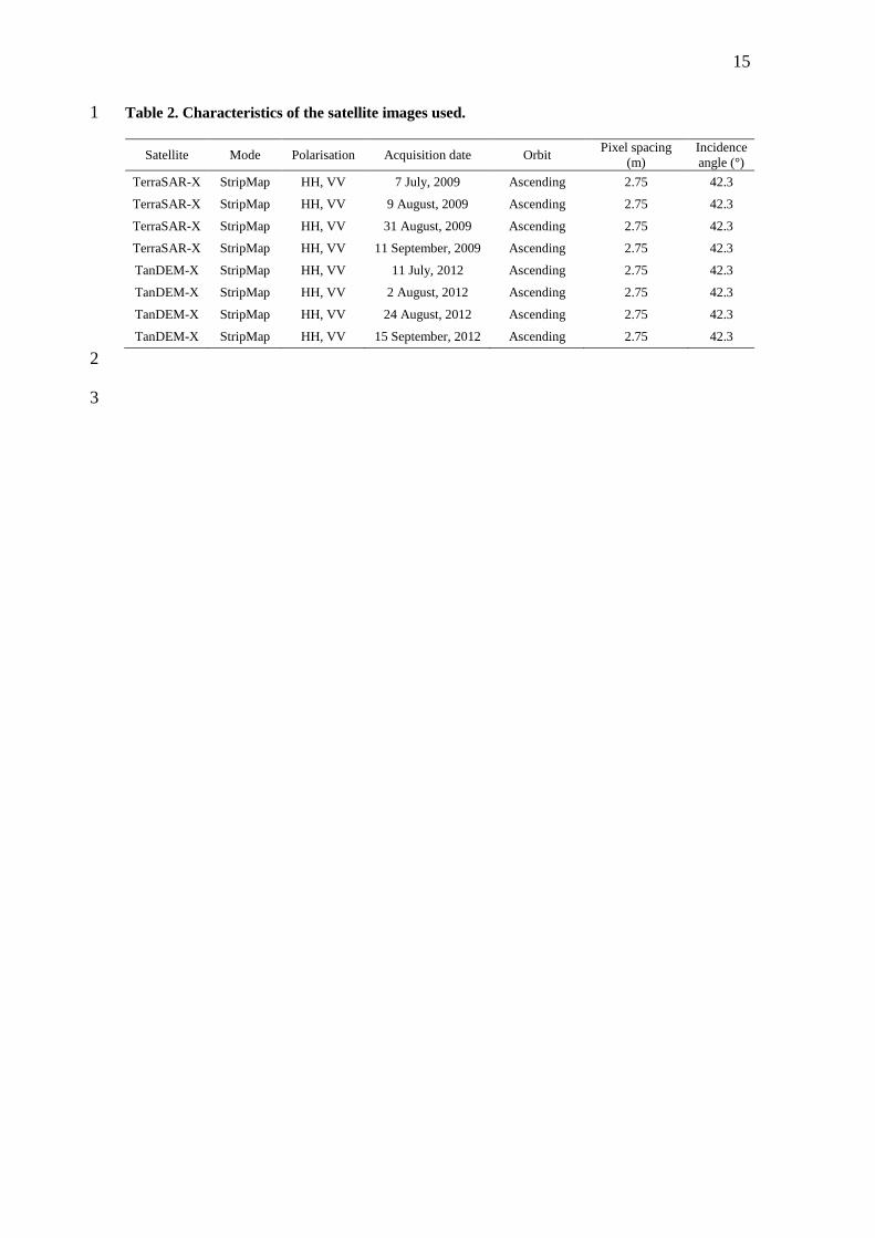
X-band SAR (TerraSAR-X or TanDEM-X) data were acquired on 7 July, 9 August, 31 13

August and 11 September, 2009, and on 11 July, 2 August, 24 August and 15 14

September, 2012 (Table 2). The SAR used in this study area was side-looking SARs 15

based on active phased-array antenna technology that flies in a sun-synchronous dawn-16

dusk orbit with an 11-day repeat at an altitude of 514 km at the equator (Roth et al. 17

2004). Multi-temporal sigma naught data have been revealed to be effective for crop 18

type classification (Bargiel and Herrmann 2011). Therefore, in this study, L1B 19

enhanced ellipsoid corrected products operated in StripMap mode were converted from 20

digital numbers to gamma naught. Then, the mean gamma naught values were 21

calculated for fields for each observation day using field polygons (shape file format) 22

provided by Tokachi Nosai (http://www.tokachi-nosai.or.jp/). These processes were 23

conducted using ERDAS IMAGINE version 14.0 distributed by Intergraph Corporation. 24

6

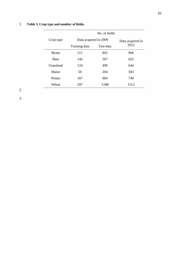
Table 3 represents the numbers of fields of each crop type. 1

<Table 2> 2

< Table 3> 3

3.2 Classification algorithm and evaluation 4

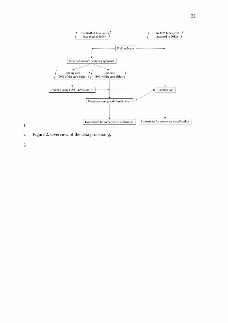
We used multi-temporal backscatter coefficients for crop classification, and the whole 5

processing workflow is illustrated in Figure 2. These classification algorithms were 6

applied using R, which provides a wide variety of statistical (linear and nonlinear 7

modelling, classical statistical tests, time-series analysis, classification, clustering) and 8

graphical techniques, and is highly extensible (R Core Team 2013). 9

<Figure 2> 10

In earlier studies, the classification and regression tree (CART) was used to identify 11

crops among alfalfa, corn, cotton, grain, melon orchards and sorghum from Landsat 12

Thematic Mapper (TM) image data, achieving overall accuracies of 87 to 92% for the 13

data acquired in 2008. Furthermore, using training data from one year and applying that 14

data to another year for classification purposes demonstrated that overall accuracies 15

from 71% to 83% are achievable, although accuracies were consistently greater than 16

85% for some crops (Hartfield et al. 2013). In addition to CART, two widely used 17

supervised learning models, the support vector machine (Bovolo et al. 2010; Foody and 18

Mathur 2004; Lizarazo 2008; Pal 2008) and random forest (Duro et al. 2012; Gislason 19

et al. 2006; Kavzoglu and Colkesen 2013; Pal 2005; Rodriguez-Galiano et al. 2012), 20

were performed in this study. 21

SVM builds a model that predicts target values when only the attributes are 22

known. The optimisation problem is solved by mapping the samples into a higher-23

dimensional space using kernel functions. Instead of modelling probability densities, 24

7

SVM uses the marginal sample and most discriminative samples (Cortes and Vapnik 1

1995). SVM provides sparse models where only a small number of samples are 2

assigned non-zero weights. These samples, called Support Vectors (SV), lie close to the 3

decision surface. The weights or coefficients used in the discriminant function are 4

obtained by maximising a margin criterion (Lizarazo 2008). The Gaussian Radial Basis 5

Function (RBF) kernel was applied (Scholkopf et al. 1997), and the two parameters C 6

and γ were tuned using a grid search in this study. The γ parameter defines how far the 7

influence of a single training sample reaches, with low values meaning ‘far’ and high 8

values meaning ‘close’. The C parameter trades off misclassification of training samples 9

against simplicity of the classification boundaries. A low C makes the classification 10

boundaries smooth, whereas a high C aims at classifying all training examples correctly. 11

RF is an ensemble learning technique that builds multiple trees based on random 12

bootstrapped samples of the training data (Breiman 2001). Each tree is built using a 13

different subset from the original training data, containing approximately two thirds of 14

the cases, and the nodes are split using the best split variable among a subset of m 15

randomly selected variables (Liaw and Wiener 2002). Through this strategy, RF is 16

robust to over-fitting and can handle thousands of input variables (dependent or 17

independent) without variable deletion (Breiman 2001). The output is determined by a 18

majority vote of the trees. Two user-defined parameters are the number of trees (k) and 19

the number of variables used to split the nodes (m); when the number of trees is 20

increased, the generalisation error always converges, and over-training is not a problem. 21

On the other hand, a reduction in the number m of predictive variables results in each 22

individual tree of the model being weaker; therefore, picking a large number of trees is 23

recommended, as is using the square root of the number of variables for the value of m 24

(Breiman 2001). 25

8

These classifications algorithms were applied using R (R Core Team 2013), 1

'rpart' package (Therneau et al. 2013), 'randomForest' package (Liaw and Wiener 2002) 2

and 'kernlab' package (Karatzoglou et al. 2013). All fields were buffered inward by 10 3

m, accounting for field shape. The buffer was used to avoid selecting training pixels 4

from the edge of a field, which would create a mixed signal and affect the accuracy 5

assessment. 6

We used a stratified random-sampling approach to select the fields used for 7

training. Approximately 20% of the crop fields were selected at random as training 8

samples. The number of samples for each crop type was determined based on the 9

percentage of fields in the area. The remaining 80% of fields were used to perform the 10

accuracy assessment. 11

Classification was performed using the training data in 2009 to classify the test 12

data in 2009 (same-year classification). Furthermore, analysis of the cross-year training 13

and classification was performed using the training data in 2009 to classify the data in 14

2012 (cross-year classification). Therefore, the crop types of training plots have not 15

changed for the data in 2012. In this study, the selected classification algorithms were 16

classification and regression tree (CART), support-vector machine (SVM) and random 17

forests (RF). 18

The classification maps were evaluated in terms of their overall accuracy (OA), 19

producer’s accuracy (PA) and user’s accuracy (UA). Furthermore, the two simple 20

measures of quantity disagreement (QD) and allocation disagreement (AD), which are 21

much more useful to summarise a cross-tabulation matrix than the kappa index of 22

agreement, were used for evaluation (Pontius and Millones 2011). The significant 23

differences among the results were determined at the 95% level of significance using 24

the Z-test, which was performed for a pairwise comparison of the proposed methods and 25

9

accounted for the ratio between the difference values of two kappa coefficients and the 1

difference in their respective variances (Congalton and Green 2008). 2

4. Results and discussion 3

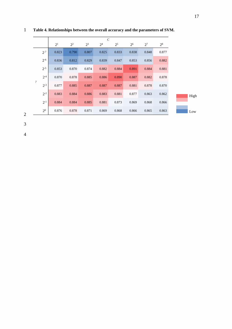
To apply SVM, the optimal values of the two parameters, C and γ, were examined. 4

Table 4 represents the relationships between the two parameters and overall accuracy of 5

the same-year classifications. The higher accuracy observed in the central range of C 6

and γ indicates that nearby same power combination but with opposite sign leads to 7

higher classification accuracy in Table 4. Thus, the parameter pair (C, γ) = (2-5，26) was 8

chosen as the optimal parameters in this study. 9

<Table 4> 10

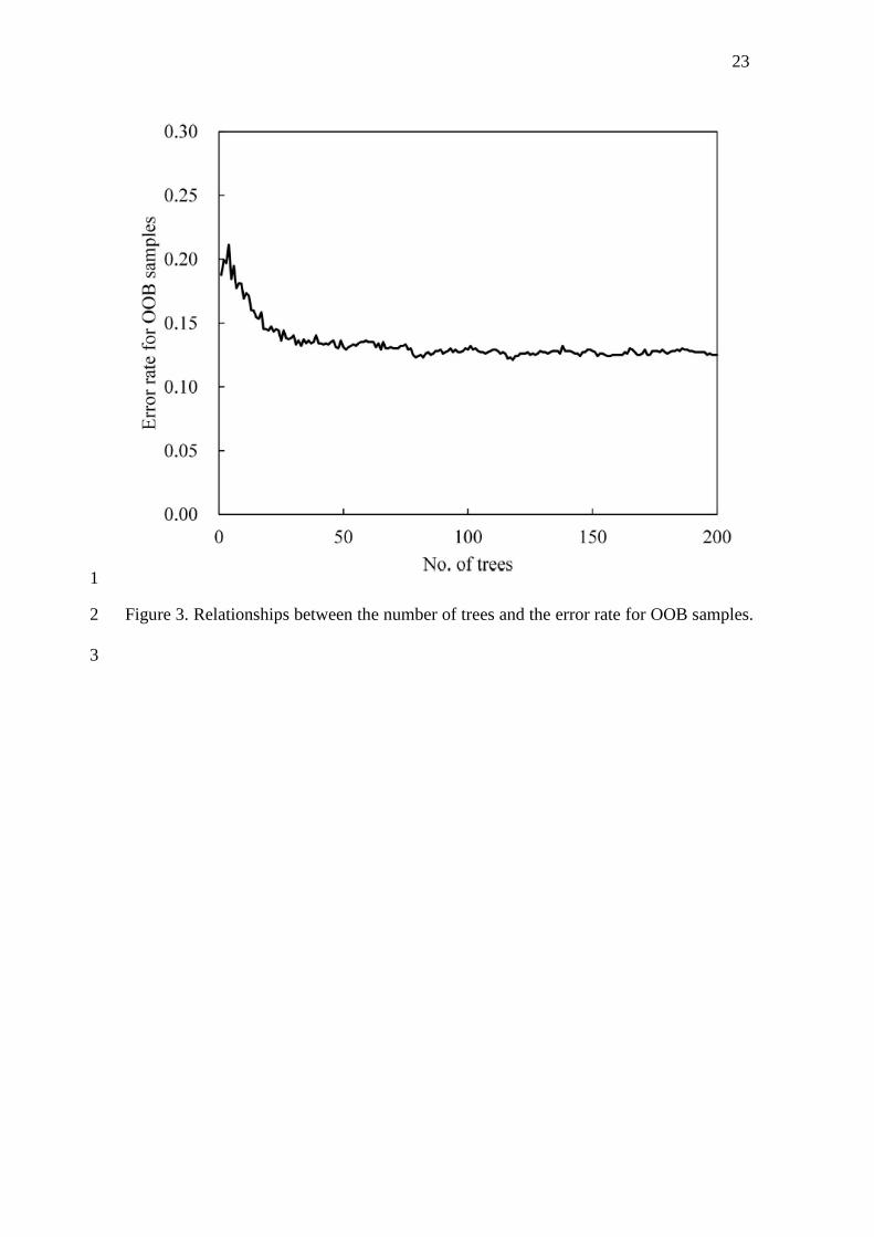
For application of RF, the number of trees was tuned, and Figure 3 represents 11

the relationships between the number of trees and the error rate for OOB. Because the 12

results indicate that a number of more than 50 is suitable, 50 was chosen as the number 13

of trees in this study. 14

<Figure 3> 15

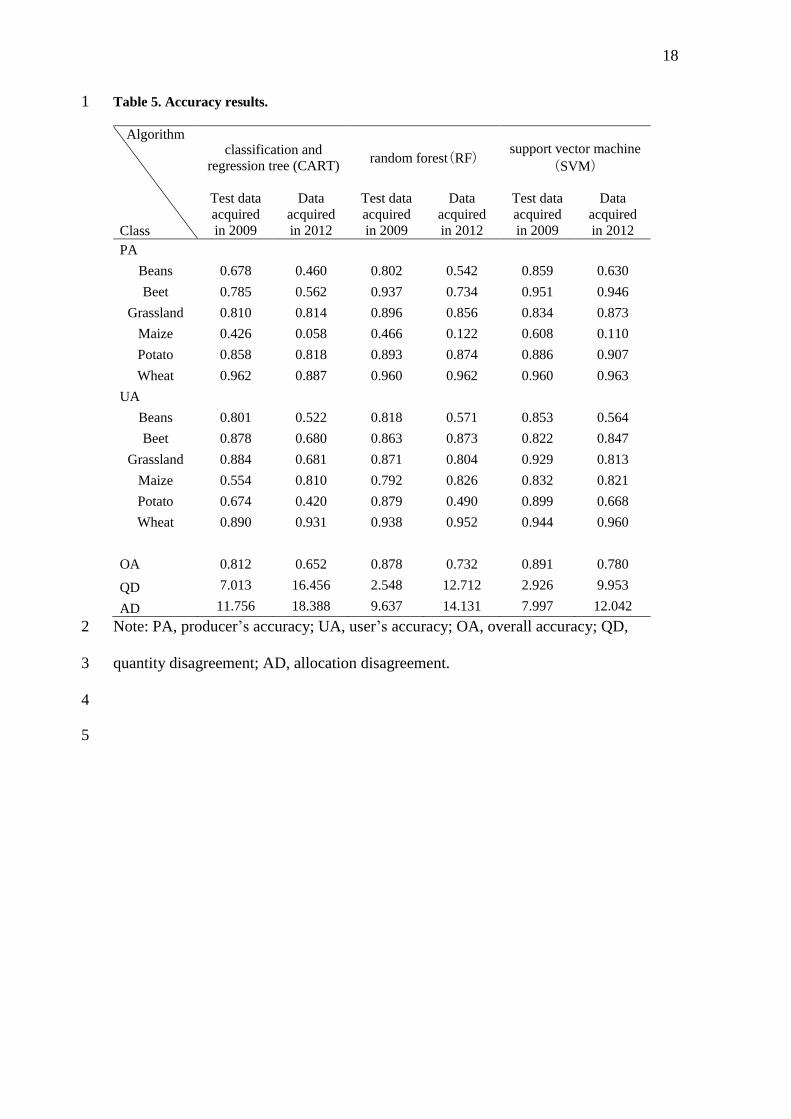
The corresponding confusion matrixes of classifications using TerraSAR-X data are 16

given in Table 5, and SVM was the best classification algorithm for the both 17

classifications. Although it is impossible to compare the results with earlier studies due 18

to the different study area and the crop types, the overall accuracies of the same year 19

classification are close to the results using backscatter data of three ENVISAT/ASAR 20

data and TerraSAR-X data for crop classification in the North China Plain (Jia et al. 21

2012). 22

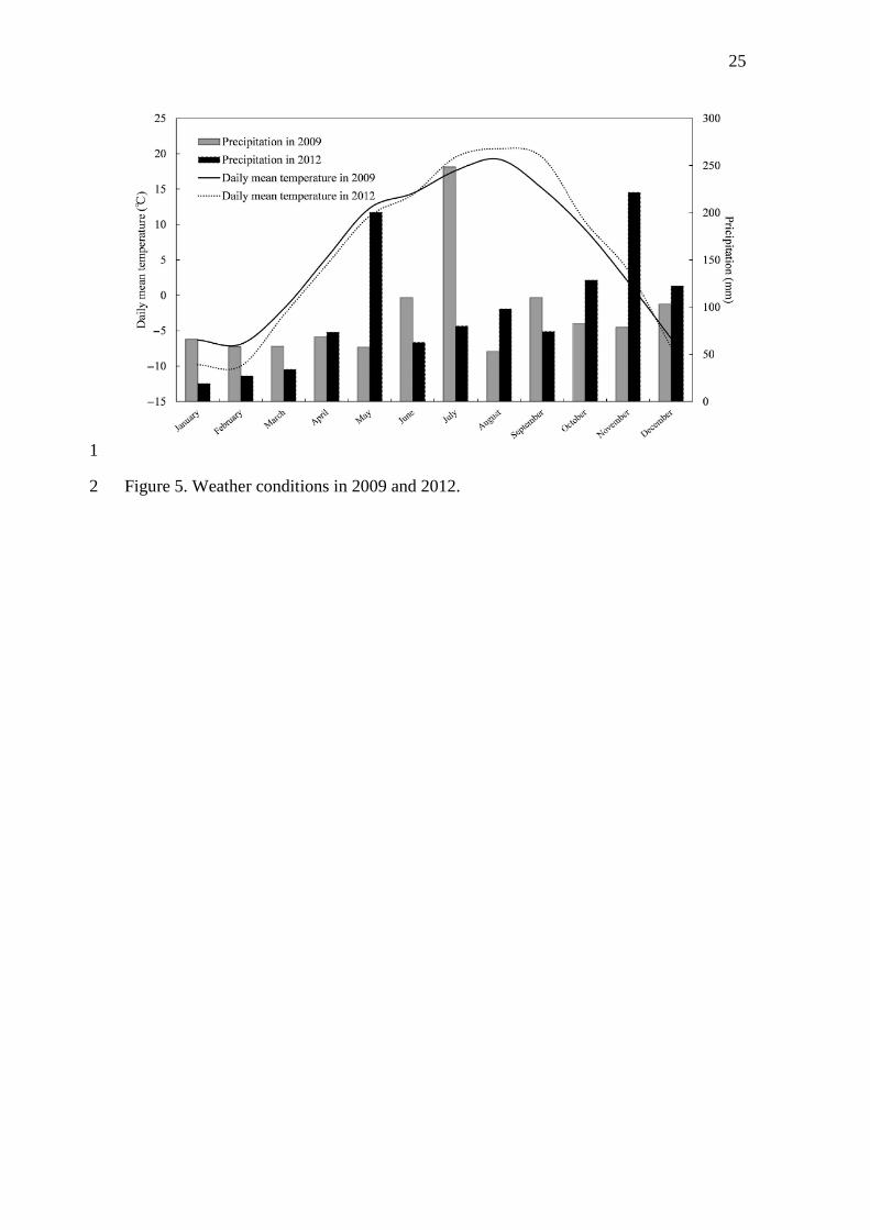
Figure 5 represents the weather conditions in 2009 and 2012. The harvesting 23

periods of winter wheat were approximately the same, regardless of the difference in the 24

climate conditions. Thus, the PAs and UAs in the cross-year classification were more 25

10

than 88 % for wheat. For other crops, in 2012, due to the higher air temperature in 1

August to September, the crop growth was advanced 2-5 days earlier than in the normal 2

year, whereas the crop growth was delayed 2-7 days in 2009, according to the 3

announcements by Tokachi Subprefecture 4

(http://www.tokachi.pref.hokkaido.lg.jp/ss/nkc/). In particular, the difference in the 5

growing conditions was large for maize (8 days). To make matters worse, in September 6

the acquisition date in 2012 was 4 days later than that in 2010. The PAs and UAs in the 7

cross-year classification were very low. Nevertheless, the overall accuracy of the cross-8

year classification using RF or SVM was close to that of Hartfield et al. (2013), which 9

indicated 71-83% using Landsat Thematic Mapper (TM) image data. 10

We used the Z-test to compare the accuracy of the classification methods 11

because the same samples and the same assessment points were used for each 12

classification. The CART, SVM and RF classifications were compared to determine 13

whether they produced significantly different results, as shown in Table 6. Based on a 14

comparison of the overall accuracies, the SVM and RF algorithms were the most 15

accurate for same-year classification because the difference between SVM and RF was 16

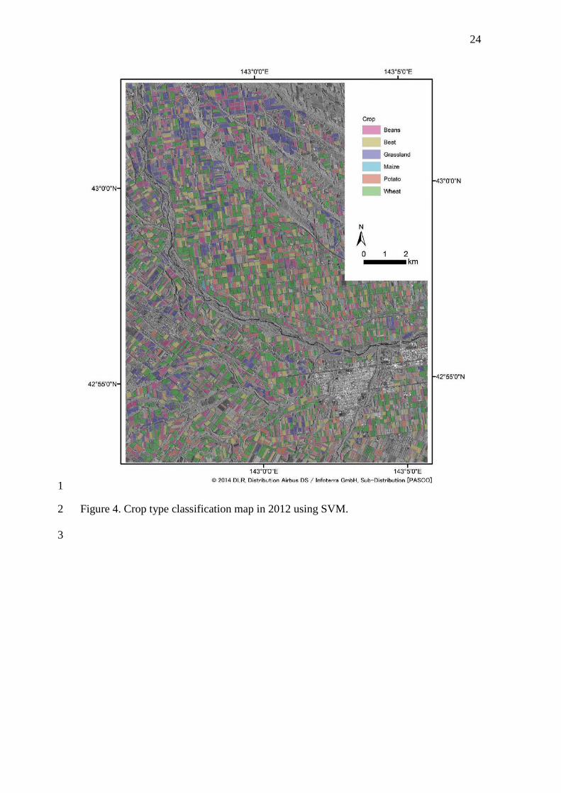
not meaningful (p< 0.05), as shown in Table 4. However, in the case of cross-year 17

classification, these algorithms differed from each other, and the SVM algorithm was 18

the most accurate (Figure 4). 19

<Table 5> 20

<Table 6> 21

<Figure 4> 22

5. Conclusions 23

To generate classification maps, in this study, three StripMap images from TerraSAR-X 24

were used, and three algorithms, CART, SVM and RF, were applied. SVM was the best 25

11

classification algorithm for both classifications in terms of OA, QD and AD, and the 1

difference of the cross-year classification result was meaningful (p< 0.05). Using the 2

training data from one year and applying those data to another year for classification 3

purposes resulted in an overall accuracy of 78.0%. 4

These results allow for the automatic and consistent crop type classifications for 5

the six defined classes. The approach offers possibilities to generate crop classification 6

maps to estimate the amount of crops harvested or agricultural disaster compensation 7

with little human power, which has significant cost. Interpretation of the entropy-alpha 8

decomposition may improve the accuracy of the classification due to understanding of 9

the scattering mechanism. In future studies, the potential of the entropy-alpha 10

decomposition for crop type classification will be tested. 11

Acknowledgements 12

This work was supported by JSPS KAKENHI Grant Number 26･5253. The field data 13

were provided by Tokachi Nosai (http://www.tokachi-nosai.or.jp/). 14

Finally, many thanks to Prof. Michael Collins and the three anonymous 15

reviewers for their important insights, which improved this article. 16

17

References 18

Ager, T.P. and P.C. Bresnahan. 2009. Geometric precision in space radar imaging: 19

Results from TerraSAR-X. In ASPRS 2009 annual conference, 9-13. Baltimore, 20

Maryland, USA. 21

Bargiel, D. and S. Herrmann. 2011. Multi-temporal land-cover classification of 22

agricultural areas in two European regions with high resolution spotlight 23

TerraSAR-X data. Remote Sensing 3, no 5: 859-877. 24

Beriaux, E., C. Lucau-Danila, E. Auquiere and P. Defourny. 2013. Multiyear 25

independent validation of the water cloud model for retrieving maize leaf area 26

index from SAR time series. International Journal of Remote Sensing 34, no 12: 27

4156-4181. 28

Blaes, X. and P. Defourny. 2003. Retrieving crop parameters based on tandem ERS 1/2 29

interferometric coherence images. Remote Sensing of Environment 88, no 4: 30

374-385. 31

12

Blaes, X., P. Defourny, U. Wegmuller, A. Della Vecchia, L. Guerriero and P. Ferrazzoli. 1

2006. C-band polarimetric indexes for maize monitoring based on a validated 2

radiative transfer model. IEEE Transactions on Geoscience and Remote Sensing 3

44, no 4: 791-800. 4

Bovolo, F., L. Bruzzone and L. Carlin. 2010. A novel technique for subpixel image 5

classification based on support vector machine. IEEE Transactions on Image 6

Processing 19, no 11: 2983-2999. 7

Breiman, L. 2001. Random forests. Machine Learning 45, no 1: 5-32. 8

Brisco, B., A. Schmitt, K. Murnaghan, S. Kaya and A. Roth. 2013. SAR polarimetric 9

change detection for flooded vegetation. International Journal of Digital Earth 6, 10

no 2: 103-114. 11

Choudhury, I. and M. Chakraborty. 2006. SAR signature investigation of rice crop 12

using radarsat data. International Journal of Remote Sensing 27, no 3: 519-534. 13

Congalton, R.G. and K. Green. 2008. Assessing the accuracy of remotely sensed data: 14

Principles and practices. Boca Raton, Florida, United States: CRC Press. 15

Cortes, C. and V. Vapnik. 1995. Support-vector networks. Machine Learning 20, no 3: 16

273-297. 17

Costa, M. P. F. 2004. Use of SAR satellites for mapping zonation of vegetation 18

communities in the Amazon floodplain. International Journal of Remote 19

Sensing, 25, no 10:1817-1835. 20

Duro, D., S. Franklin and M. Dube. 2012. Multi-scale object-based image analysis and 21

feature selection of multi-sensor earth observation imagery using random forests. 22

International Journal of Remote Sensing 33, no 14: 4502-4526. 23

Fontanelli, G., S. Paloscia, M. Zribi and A. Chahbi. 2013. Sensitivity analysis of X-24

band SAR to wheat and barley leaf area index in the merguellil basin. Remote 25

Sensing Letters 4, no 11: 1107-1116. 26

Foody, G. and A. Mathur. 2004. A relative evaluation of multiclass image classification 27

by support vector machines. IEEE Transactions on Geoscience and Remote 28

Sensing 42, no 6: 1335-1343. 29

Gislason, P., J. Benediktsson and J. Sveinsson. 2006. Random forests for land cover 30

classification. Pattern Recognition Letters 27, no 4: 294-300. 31

Hartfield, K., S. Marsh, C. Kirk and Y. Carriere. 2013. Contemporary and historical 32

classification of crop types in Arizona. International Journal of Remote Sensing 33

34, no 17: 6024-6036. 34

Jia, K., Q. Li, Y. Tian, B. Wu, F. Zhang and J. Meng. 2012. Crop classification using 35

multi-configuration SAR data in the North China Plain International Journal of 36

Remote Sensing 33, no 1: 170-183. 37

Karatzoglou, A., A. Smola and K. Hornik. Package ‘kernlab’. http://cran.r-38

project.org/web/packages/kernlab/kernlab.pdf. 39

Kavzoglu, T. and I. Colkesen. 2013. An assessment of the effectiveness of a rotation 40

forest ensemble for land-use and land-cover mapping. International Journal of 41

Remote Sensing 34, no 12: 4224-4241. 42

Kuenzer, C. and K. Knauer. 2013. Remote sensing of rice crop areas. International 43

Journal of Remote Sensing 34, no 6: 2101-2139. 44

Liaw, A. and M. Wiener. 2002. Classification and regression by random forest. R News 45

2, no 3: 18-22. 46

Lievens, H. and N. Verhoest. 2011. On the retrieval of soil moisture in wheat fields 47

from L-band SAR based on water cloud modeling, the IEM, and effective 48

roughness parameters. IEEE Geoscience and Remote Sensing Letters 8, no 4: 49

740-744. 50

13

Lizarazo, I. 2008. Svm-based segmentation and classification of remotely sensed data. 1

International Journal of Remote Sensing 29, no 24: 7277-7283. 2

Mattia, F., T. Le Toan, G. Picard, F. Posa, A. D'alessio, C. Notarnicola, A. Gatti, M. 3

Rinaldi, G. Satalino and G. Pasquariello. 2003. Multitemporal C-band radar 4

measurements on wheat fields. IEEE Transactions on Geoscience and Remote 5

Sensing 41, no 7: 1551-1560. 6

Mishra, N.B. and K.A. Crews. 2014. Mapping vegetation morphology types in a dry 7

savanna ecosystem: Integrating hierarchical object-based image analysis with 8

random forest. International Journal of Remote Sensing 35, no 3: 1175-1198. 9

Otsu, N. 1979. A threshold selection method from gray-level histograms. IEEE 10

Transactions on Systems, Man, and Cybernetics 9 no 1, 62-66. 11

Pal, M. 2005. Random forest classifier for remote sensing classification. International 12

Journal of Remote Sensing 26, no 1: 217-222. 13

Pal, M. 2008. Ensemble of support vector machines for land cover classification. 14

International Journal of Remote Sensing 29, no 10: 3043-3049. 15

Pontius, R. and M. Millones. 2011. Death to kappa: Birth of quantity disagreement and 16

allocation disagreement for accuracy assessment. International Journal of 17

Remote Sensing 32, no 15: 4407-4429. 18

R Core Team. 2013. A Language and Environment for Statistical Computing. Vienna: R 19

Foundation for Statistical Computing. Accessed October 11. http://www.R-20

project.org/ 21

Rodriguez-Galiano, V., M. Chica-Olmo, F. Abarca-Hernandez, P. Atkinson and C. 22

Jeganathan. 2012. Random forest classification of mediterranean land cover 23

using multi-seasonal imagery and multi-seasonal texture. Remote Sensing of 24

Environment 121: 93-107. 25

Roth, A., M. Huber and D. Kosmann. 2004. Geocording of TerraSAR-X data. In 20th 26

ISPRS Congress, 840-844. Istanbul. 27

Sarker, L. and J. Nichol. 2011. Improved forest biomass estimates using alos avnir-2 28

texture indices. Remote Sensing of Environment 115, no 4: 968-977. 29

Scholkopf, B., K. Sung, C. Burges, F. Girosi, P. Niyogi, T. Poggio and V. Vapnik. 1997. 30

Comparing support vector machines with gaussian kernels to radial basis 31

function classifiers. IEEE Transactions on Signal Processing 45, no 11: 2758-32

2765. 33

Sonobe, R., H. Tani, X. Wang, N. Kobayashi and H. Shimamura. 2014a. Random forest 34

classification of crop type using multi-temporal TerraSAR-X dual-polarimetric 35

data. Remote Sensing Letters 5, no 2: 157-1564. 36

Sonobe, R., H. Tani, X. Wang, N. Kobayashi, A. Kimura and H. Shimamura. 2014b. 37

Application of multi-temporal TerraSAR-X data to map winter wheat planted 38

areas in Hokkaido, Japan. Japan Agricultural Research Quarterly 48, no 4: 465-39

470. 40

Sonobe, R., H. Tani, X. Wang, N. Kobayashi and H. Shimamura. 2014c. Winter wheat 41

growth monitoring using multi-temporal TerraSAR-X dual-polarimetric data. 42

Japan Agricultural Research Quarterly 48, no 4: 471-476. 43

Therneau, T., B. Atkinson and B. Riple. Package ‘rpart’. http://cran.r-44

project.org/web/packages/rpart/rpart.pdf. 45

Ulaby, F.T., M.K. Moore and A.K. Fung. 1986. Microwave remote sensing active and 46

passive. Norwood: Artech House. 47

Vyas, S., M. Steven, K. Jaggard and H. Xu. 2003. Comparison of sugar beet crop cover 48

estimates from radar and optical data. International Journal of Remote Sensing 49

24, no 5: 1071-1082. 50 51

14

Table 1. Cultivation calendar for the crops in this study area. 1

May

Bean

s

Beet

Gra

ssla

nd

Maiz

e

Po

tato

Wh

eat

so

win

g

Jun

eJu

lyA

ug

ust

sp

rou

tin

g

sp

rou

tin

g

2n

d h

arv

esti

ng

sp

rou

tin

gp

lan

tin

g

ap

peara

nce o

f ears

of

gra

inh

arv

esti

ng

harv

esti

ng

harv

esti

ng

Octo

ber

ap

peara

nce o

f ta

ssel

harv

esti

ng

harv

esti

ng

Sep

tem

ber

so

win

g

so

win

g

ap

peara

nce o

f ears

of

gra

in1st

harv

esti

ng

2

3

15

Table 2. Characteristics of the satellite images used. 1

Satellite Mode Polarisation Acquisition date Orbit Pixel spacing

(m)

Incidence

angle (°)

TerraSAR-X StripMap HH, VV 7 July, 2009 Ascending 2.75 42.3

TerraSAR-X StripMap HH, VV 9 August, 2009 Ascending 2.75 42.3

TerraSAR-X StripMap HH, VV 31 August, 2009 Ascending 2.75 42.3

TerraSAR-X StripMap HH, VV 11 September, 2009 Ascending 2.75 42.3

TanDEM-X StripMap HH, VV 11 July, 2012 Ascending 2.75 42.3

TanDEM-X StripMap HH, VV 2 August, 2012 Ascending 2.75 42.3

TanDEM-X StripMap HH, VV 24 August, 2012 Ascending 2.75 42.3

TanDEM-X StripMap HH, VV 15 September, 2012 Ascending 2.75 42.3

2

3

16

Table 3. Crop type and number of fields. 1

Crop type

No. of fields

Data acquired in 2009 Data acquired in

2012 Training data Test data

Beans 211 842 960

Beet 142 567 625

Grassland 124 499 644

Maize 50 204 583

Potato 167 664 749

Wheat 297 1188 1513

2

3

17

Table 4. Relationships between the overall accuracy and the parameters of SVM. 1

0.823 0.790 0.807 0.825 0.833 0.838 0.848 0.877

0.836 0.812 0.829 0.839 0.847 0.853 0.856 0.882

0.853 0.870 0.874 0.882 0.884 0.891 0.884 0.881

0.870 0.878 0.885 0.886 0.890 0.887 0.882 0.878

0.877 0.885 0.887 0.887 0.887 0.881 0.878 0.870

0.883 0.884 0.886 0.883 0.881 0.877 0.863 0.862

0.884 0.884 0.885 0.881 0.873 0.869 0.868 0.866

0.876 0.878 0.871 0.869 0.868 0.866 0.865 0.863

C

γ

21 22 23 24 25 26 27 28

20

2-1

2-2

2-3

2-4

2-5

2-6

2-7

210

-1-2

High

Low 2

3

4

18

Table 5. Accuracy results. 1

Algorithm

Class

classification and

regression tree (CART) random forest（RF）

support vector machine

（SVM）

Test data

acquired

in 2009

Data

acquired

in 2012

Test data

acquired

in 2009

Data

acquired

in 2012

Test data

acquired

in 2009

Data

acquired

in 2012

PA

Beans 0.678 0.460 0.802 0.542 0.859 0.630

Beet 0.785 0.562 0.937 0.734 0.951 0.946

Grassland 0.810 0.814 0.896 0.856 0.834 0.873

Maize 0.426 0.058 0.466 0.122 0.608 0.110

Potato 0.858 0.818 0.893 0.874 0.886 0.907

Wheat 0.962 0.887 0.960 0.962 0.960 0.963

UA

Beans 0.801 0.522 0.818 0.571 0.853 0.564

Beet 0.878 0.680 0.863 0.873 0.822 0.847

Grassland 0.884 0.681 0.871 0.804 0.929 0.813

Maize 0.554 0.810 0.792 0.826 0.832 0.821

Potato 0.674 0.420 0.879 0.490 0.899 0.668

Wheat 0.890 0.931 0.938 0.952 0.944 0.960

OA 0.812 0.652 0.878 0.732 0.891 0.780

QD 7.013 16.456 2.548 12.712 2.926 9.953

AD 11.756 18.388 9.637 14.131 7.997 12.042

Note: PA, producer’s accuracy; UA, user’s accuracy; OA, overall accuracy; QD, 2

quantity disagreement; AD, allocation disagreement. 3

4

5

19

Table 6. Z-test results for the classification. 1

classification SVM RF

same-year CART 10.22 8.42

SVM 1.8

cross-year CART 15.49 9.61

SVM 5.83

2

3

20

Figures 1

Figure 1. The study area (background map shows the TerraSAR-X data acquired on 2 May, 2

2009). 3

4

Figure 2. Overview of the data processing. 5

6

Figure 3. Relationships between the number of trees and the error rate for OOB samples. 7

8

Figure 4. Crop type classification map in 2012 using SVM. 9

10

Figure 5. Weather conditions in 2009 and 2012.11

21

1

Figure 1. The study area (background map shows the TerraSAR-X data acquired on 2 May, 2

2009).3

22

1

Figure 2. Overview of the data processing. 2

3

23

1

Figure 3. Relationships between the number of trees and the error rate for OOB samples. 2

3

24

1

Figure 4. Crop type classification map in 2012 using SVM. 2

3

25

1

Figure 5. Weather conditions in 2009 and 2012. 2